Globe: A SAM Based Global CGE Model using GTAP Data

Globe: A SAM Based Global CGE Model using GTAP Data, May 2007

1

Globe: A SAM Based Global CGE Model using

GTAP Data

Scott McDonald, Karen Thierfelder and Sherman Robinson1

Addresses for correspondence:

Scott McDonald, Karen Thierfelder Department of Economics, Department of Economics The University of Sheffield, US Naval Academy 9 Mappin Street, Annapolis, Sheffield, S1 4DT, UK. Maryland, USA Email: [email protected] Email: [email protected] Tel: +44 114 22 23407 Tel: +1 410 293 6887 Abstract

This paper provides a technical description of a global computable general equilibrium (CGE) model that is calibrated from a Social Accounting Matrix (SAM) representation of the Global Trade Analysis Project (GTAP) database. An important feature of the model is the treatment of nominal and real exchange rates and hence the specification of multiple numéraire. Another distinctive feature of the model is the use of a ‘dummy’ region, known as globe, that allows for the recording of inter regional transactions where either the source or destination are not identified.

Keywords: Computable General Equilibrium; GTAP.

JEL classification: D58; R13; F49.

1 Scott McDonald is a Reader in Economics at the University of Sheffield; Karen Thierfelder is Professor

of Economics at the United States Naval Academy; and Sherman Robinson is Professor of Economics at the University of Sussex.

mailto:[email protected]

mailto:[email protected]


2

1. Introduction

This paper provides a technical description of a variant of a Social Accounting Matrix (SAM)

based Global Computable General Equilibrium (CGE) model that has been calibrated using

data derived from the Global Trade Analysis Project’s (GTAP) database. The model is a

member of a family of CGE models that model trade relationships using principles described

in the 1-2-3 model (de Melo and Robinson, 1989; Devarajan, et al., 1990). More specifically

this model is a direct descendant of an early US Department of Agriculture model (see

Robinson et al., 1990) and NAFTA (see Robinson et al., 1993). However numerous features

of this model stem from other developments in CGE modelling over the last 15 years; some of

these sources of inspiration are direct and easily identified, e.g., analysis used in the World

Development Report, 1995 (Lewis, Robinson, and Wang), the IFPRI standard model

(Lofgren et al., 2002) and the PROVIDE Project model (McDonald, 2003), others are indirect

and easily identified, e.g., the GTAP model (Hertel, 1997), while others are both direct and

indirect but less easily identified; a substantial debt is owed to the community of CGE

modellers. In addition the model owes a lot to the development of the SAM approach to

national accounting, e.g., Stone (1962a and b) and Pyatt (1991), and the SAM approach to

modelling, e.g., Pyatt (1987), Drud et al., (1986).

The underlying approach to multi-region modelling for this CGE model is the

construction of a series of single country CGE models that are linked through their trading

relationships. As is common with all known CGE models the price systems in the model are

linear homogenous and hence the focus is upon movements in relative, rather than absolute,

prices. Consequently each region in the model has its own numéraire price, typically the

consumer price index (CPI), and a nominal exchange rate, while the model as a whole

requires a numéraire, which is an exchange rate index for a number of reference regions. As

such this model contains a fundamentally different philosophical approach to global

modelling to that found in the GTAP model.2 Behind this difference lies a deep theoretical

debate about how comparative static and finite horizon dynamic CGE models should value

transfers associated with the capital account of the balance of payments (see Robinson, 2004).

2 The GTAP model does not contain nominal exchange rates and has a single global numéraire.


3

A distinctive feature of the model is the use of a ‘dummy’ region, known as Globe, that

allows for the recording of inter regional transactions where either the source or destination

are not identified. Examples of such transactions include trade and transportation margins and

data on remittances. The Globe construct provides a general method for dealing with any

transactions data where full bilateral information is missing.

The rest of this paper is organised as follows. Section 2 reviews the data used in the

model; this section also provides a brief description of how the data were transformed from

the GTAP database into a SAM. This is followed in section 3 by a descriptive overview of the

model and then, in section 4, by a formal description of the model’s equations. The

description in section 4 is based upon a default setting for the model closure rules; one of the

model’s key features is the flexibility of the closure rules and consequently section 5

considers the alternatives built into the model’s basic structure. All global CGE models are

large and therefore present a series of potential implementation problems; section 6 briefly

reviews some of the programmes that have been developed to support the basic model and

provides some guidelines for use of this class of model. This is followed by some concluding

comments that primarily focus upon planned model developments. Finally there are a series

of technical appendices relating to aspects of model formulation, calibration of use – details

about the content of these appendices is provided at the start of the appendices.

3. Model Data

The data used in the model were derived from the GTAP database (see Hertel, 1997) using a

three dimensional Social Accounting Matrix (SAM) method for organising the data. Details

of the method used to generate a SAM representation are reported in McDonald and

Thierfelder (2004a) while a variety of reduced form representations of the SAM and methods

for augmenting the GTAP database are reported in McDonald and Thierfelder (2004b) and

McDonald and Sonmez (2004) respectively. Detailed descriptions of the data are provided

elsewhere so the discussion here is limited to the general principles.

Global Social Accounting Matrix

The Global SAM can be conceived of as a series of single region SAMs that are linked

through the trade accounts; it is particularly valid in the context of the GTAP database to note


4

that the ONLY way in which the regions are linked directly in the database is through

commodity trade transactions although there are some indirect links through the demand and

supply of trade and transport services. Specifically the value of exports, valued free on board

(fob) from source x to destination y must be exactly equal to the value of imports valued fob

to destination y from source x, and since this holds for all commodity trade transactions the

sum of the differences in the values of imports and exports by each region must equal zero.

However the resultant trade balances do not fully accord with national accounting

conventions because other inter regional transactions are not recorded in the database (see

McDonald and Sonmez, 2004). A description of the transactions recorded in a representative

SAM for a typical region in the database is provided in Table 1.

A SAM is a transactions matrix; hence each cell in a SAM simply records the values of

the transactions between the two agents identified by the row and column accounts. The

selling agents are identified by the rows, i.e., the row entries record the incomes received by

the identified agent, while the purchasing agents are identified by the columns, i.e., the

column entries record the expenditures made by agents. As such a SAM is a relatively

compact form of double entry bookkeeping that is complete and consistent and can be used to

present the National Accounts of a country in a single two-dimensional matrix (see UN, 1993,

for a detailed explanation of the relationship between conventional and SAM presentations of

National Accounts). A SAM is complete in the sense that the SAM should record ALL the

transactions within the production boundary of the National Accounts, and consistent in the

sense that income transactions by each and every agent are exactly matched by expenditure

transactions of other agents. A fundamental consequence of these conditions is that the row

and column totals of the SAM for each region must be identical, and hence the SAM provides

a complete characterisation of current account transactions of an economy as a circular (flow)

system. In the context of a global SAM the complete and consistent conditions need

extending to encompass transactions between regions; this simply requires that each and

every import transaction by a region must have an identical counterpart export transaction by

another region. This is enough to ensure that the resultant global SAM provides a

characterisation of current account transactions of the global economy as a circular (flow)

system.


5

Table 1 Social Accounting Matrix for a Region in the Global Social Accounting Matrix

Commodities Activities Factors Households Government Capital Margins Rest of World Totals

Commodities 0 Combined

Intermediate Use Matrix

0 Private Consumption

Government Consumption

Investment Consumption

Exports of Margins(fob)

Exports of Commodities (fob)

Total Demand for Commodities

Activities Domestic Supply Matrix 0 0 0 0 0 0 0 Total Domestic

Supply by Activity

Factors 0 Expenditure on Primary Inputs 0 0 0 0 0 0 Total Factor

Income

Households 0 0 Distribution of Factor Incomes 0 0 0 0 0 Total Household

Income

Government Taxes on Commodities

Taxes on Production

Taxes on Factor Use

Direct/Income Taxes

Direct/Income Taxes 0 0 0 0 Total Government

Income

Capital 0 0 Depreciation Allowances Household Savings Government

Savings 0 Balance on Margins Trade Foreign Savings Total Savings

Margins Imports of Trade

and Transport Margins

0 0 0 0 0 0 0 Total Income from Margin Imports

Rest of World

Imports of Commodities (fob) 0 0 0 0 0 0 0 Total Income from

Imports

Totals Total Supply of Commodities

Total Expenditure on Inputs by

Activities

Total Factor Expenditure

Total Household Expenditure

Total Government Expenditure Total Investment Total Expenditure

on Margin ExportsTotal Expenditure

on Exports


6

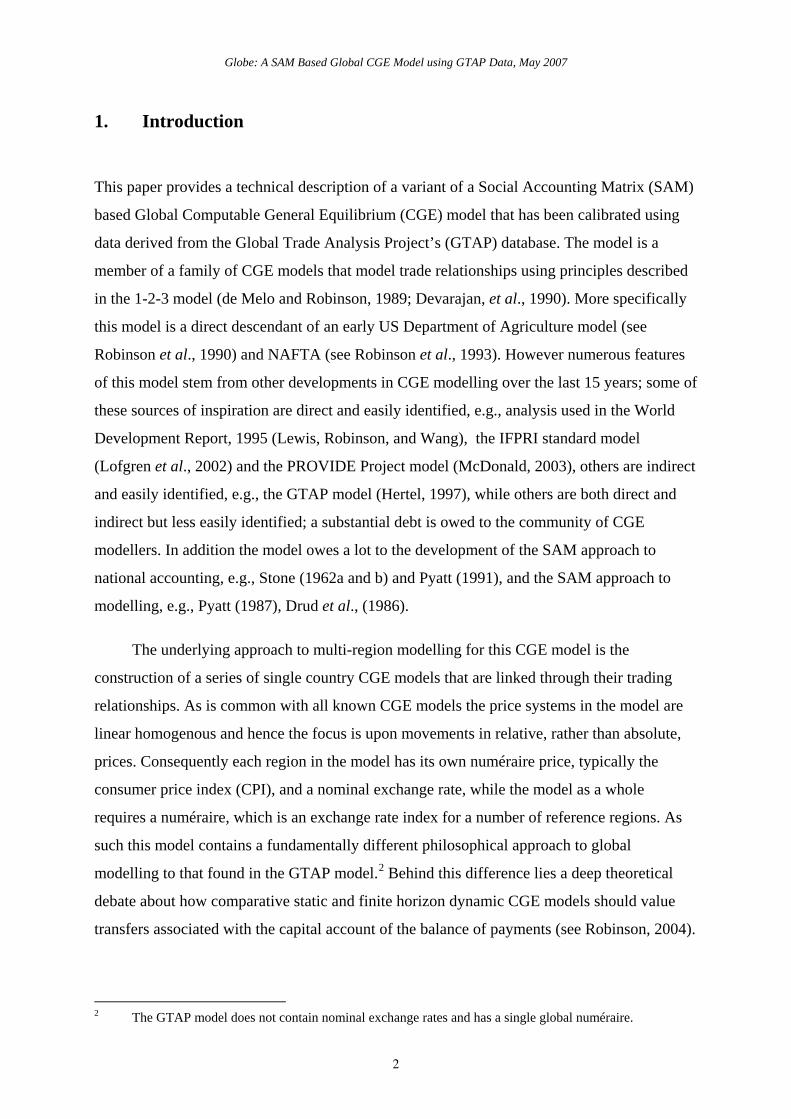
Given these definitions of a SAM the transactions recorded in a SAM are easily

interpreted. In Table 1 the row entries for the commodity accounts are the values of

commodity sales to the agents identified in the columns, i.e., intermediate inputs are

purchased by activities (industries etc.,), final consumption is provided by households, the

government and investment demand and export demand is provided by the all the other

regions in the global SAM and the export of margin services. The commodity column entries

deal with the supply side, i.e., they identify the accounts from which commodities are

purchased so to satisfy demand. Specifically commodities can be purchased from either

domestic activities – the domestic supply matrix valued inclusive of domestic trade and

transport margins – or they can be imported – valued exclusive of international trade and

transport margins. In addition to payments to the producing agents – domestic or foreign – the

commodity accounts need to make expenditures with respect to the trade and transport

services needed to import the commodities and any commodity specific taxes.

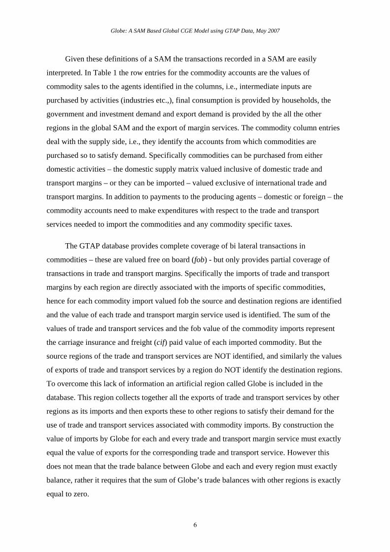
The GTAP database provides complete coverage of bi lateral transactions in

commodities – these are valued free on board (fob) - but only provides partial coverage of

transactions in trade and transport margins. Specifically the imports of trade and transport

margins by each region are directly associated with the imports of specific commodities,

hence for each commodity import valued fob the source and destination regions are identified

and the value of each trade and transport margin service used is identified. The sum of the

values of trade and transport services and the fob value of the commodity imports represent

the carriage insurance and freight (cif) paid value of each imported commodity. But the

source regions of the trade and transport services are NOT identified, and similarly the values

of exports of trade and transport services by a region do NOT identify the destination regions.

To overcome this lack of information an artificial region called Globe is included in the

database. This region collects together all the exports of trade and transport services by other

regions as its imports and then exports these to other regions to satisfy their demand for the

use of trade and transport services associated with commodity imports. By construction the

value of imports by Globe for each and every trade and transport margin service must exactly

equal the value of exports for the corresponding trade and transport service. However this

does not mean that the trade balance between Globe and each and every region must exactly

balance, rather it requires that the sum of Globe’s trade balances with other regions is exactly

equal to zero.


7

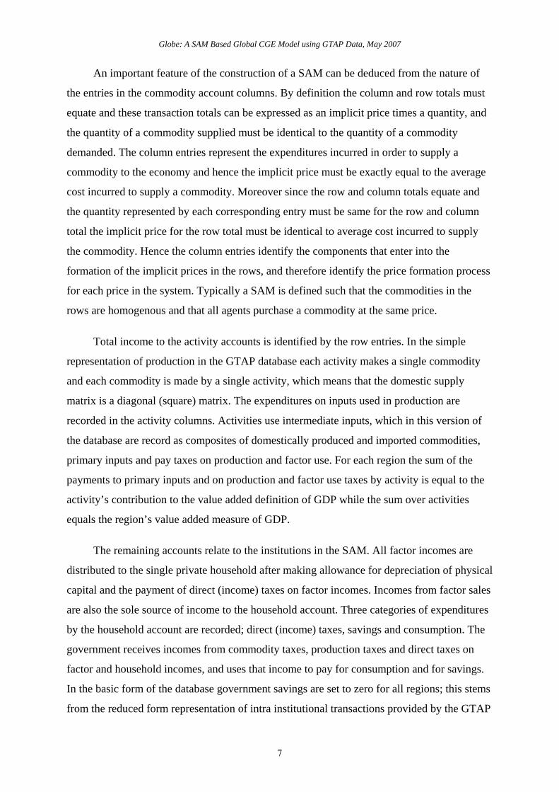
An important feature of the construction of a SAM can be deduced from the nature of

the entries in the commodity account columns. By definition the column and row totals must

equate and these transaction totals can be expressed as an implicit price times a quantity, and

the quantity of a commodity supplied must be identical to the quantity of a commodity

demanded. The column entries represent the expenditures incurred in order to supply a

commodity to the economy and hence the implicit price must be exactly equal to the average

cost incurred to supply a commodity. Moreover since the row and column totals equate and

the quantity represented by each corresponding entry must be same for the row and column

total the implicit price for the row total must be identical to average cost incurred to supply

the commodity. Hence the column entries identify the components that enter into the

formation of the implicit prices in the rows, and therefore identify the price formation process

for each price in the system. Typically a SAM is defined such that the commodities in the

rows are homogenous and that all agents purchase a commodity at the same price.

Total income to the activity accounts is identified by the row entries. In the simple

representation of production in the GTAP database each activity makes a single commodity

and each commodity is made by a single activity, which means that the domestic supply

matrix is a diagonal (square) matrix. The expenditures on inputs used in production are

recorded in the activity columns. Activities use intermediate inputs, which in this version of

the database are record as composites of domestically produced and imported commodities,

primary inputs and pay taxes on production and factor use. For each region the sum of the

payments to primary inputs and on production and factor use taxes by activity is equal to the

activity’s contribution to the value added definition of GDP while the sum over activities

equals the region’s value added measure of GDP.

The remaining accounts relate to the institutions in the SAM. All factor incomes are

distributed to the single private household after making allowance for depreciation of physical

capital and the payment of direct (income) taxes on factor incomes. Incomes from factor sales

are also the sole source of income to the household account. Three categories of expenditures

by the household account are recorded; direct (income) taxes, savings and consumption. The

government receives incomes from commodity taxes, production taxes and direct taxes on

factor and household incomes, and uses that income to pay for consumption and for savings.

In the basic form of the database government savings are set to zero for all regions; this stems

from the reduced form representation of intra institutional transactions provided by the GTAP


8

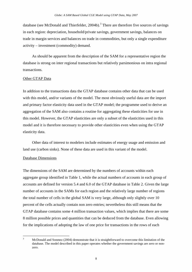
database (see McDonald and Thierfelder, 2004b).3 There are therefore five sources of savings

in each region: depreciation, household/private savings, government savings, balances on

trade in margin services and balances on trade in commodities, but only a single expenditure

activity – investment (commodity) demand.

As should be apparent from the description of the SAM for a representative region the

database is strong on inter regional transactions but relatively parsimonious on intra regional

transactions.

Other GTAP Data

In addition to the transactions data the GTAP database contains other data that can be used

with this model, and/or variants of the model. The most obviously useful data are the import

and primary factor elasticity data used in the GTAP model; the programme used to derive an

aggregation of the SAM also contains a routine for aggregating these elasticities for use in

this model. However, the GTAP elasticities are only a subset of the elasticities used in this

model and it is therefore necessary to provide other elasticities even when using the GTAP

elasticity data.

Other data of interest to modelers include estimates of energy usage and emission and

land use (carbon sinks). None of these data are used in this variant of the model.

Database Dimensions

The dimensions of the SAM are determined by the numbers of accounts within each

aggregate group identified in Table 1, while the actual numbers of accounts in each group of

accounts are defined for version 5.4 and 6.0 of the GTAP database in Table 2. Given the large

number of accounts in the SAMs for each region and the relatively large number of regions

the total number of cells in the global SAM is very large, although only slightly over 10

percent of the cells actually contain non zero entries; nevertheless this still means that the

GTAP database contains some 4 million transaction values, which implies that there are some

8 million possible prices and quantities that can be deduced from the database. Even allowing

for the implications of adopting the law of one price for transactions in the rows of each

3 McDonald and Sonmez (2004) demonstrate that it is straightforward to overcome this limitation of the

database. The model described in this paper operates whether the government savings are zero or non-zero.


9

region’s SAM and for other ways of reducing the numbers of independent prices and

quantities that need to be estimated in a modelling environment, it is clear that the use of the

GTAP database without aggregation is likely to generate extremely large models (in terms of

the number of equations/variables). Consequently, except in exceptional circumstances all

CGE models that use the GTAP data operate with aggregations of the database.

Table 2 Dimensions of the Global Social Accounting Matrix

Account Groups Sets Total Number of Accounts

GTAP 5.4 GTAP 6.0

Commodities C 57 57

Activities A 57 57

Factors F 5 5

Taxes (2*r)+(1*f)+3 164 182

Other Domestic Institutions 3 3 3

Margins 3*r 234 261

Trade R 78 87

Total 598 652

Total Number of Cells in the Global SAM 27,893,112 36,984,048

3 Overview of the Model

Behavioural Relationships

The within regional behavioural relationships are fairly standard in this variant of the model;

it is easy to make them more elaborate but the focus in this variant of the model is upon

international trade relationships. The activities are assumed to maximise profits using

technology characterised by Constant Elasticity of Substitution (CES) or Leontief production

functions between aggregate primary inputs and aggregate intermediate inputs, with CES

production functions over primary inputs and Leontief technology across intermediate inputs.

The household maximises utility subject to preferences represented by a Stone-Geary utility


10

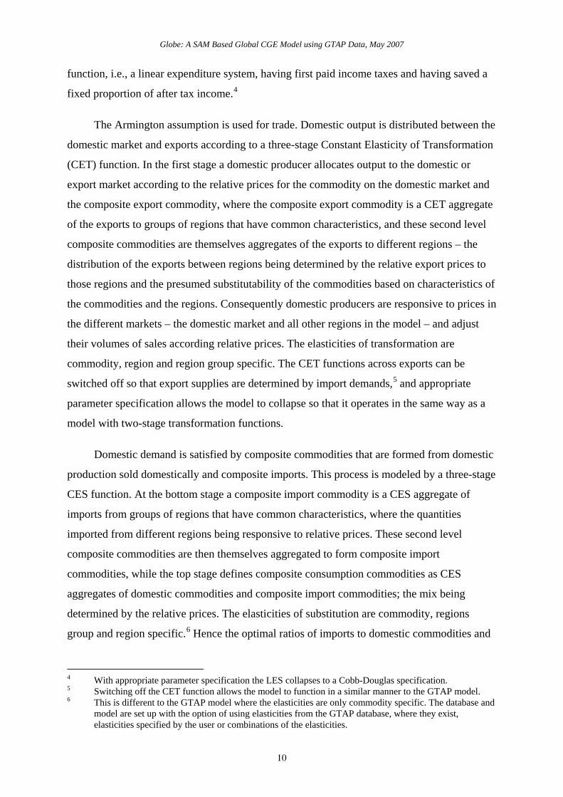
function, i.e., a linear expenditure system, having first paid income taxes and having saved a

fixed proportion of after tax income.4

The Armington assumption is used for trade. Domestic output is distributed between the

domestic market and exports according to a three-stage Constant Elasticity of Transformation

(CET) function. In the first stage a domestic producer allocates output to the domestic or

export market according to the relative prices for the commodity on the domestic market and

the composite export commodity, where the composite export commodity is a CET aggregate

of the exports to groups of regions that have common characteristics, and these second level

composite commodities are themselves aggregates of the exports to different regions – the

distribution of the exports between regions being determined by the relative export prices to

those regions and the presumed substitutability of the commodities based on characteristics of

the commodities and the regions. Consequently domestic producers are responsive to prices in

the different markets – the domestic market and all other regions in the model – and adjust

their volumes of sales according relative prices. The elasticities of transformation are

commodity, region and region group specific. The CET functions across exports can be

switched off so that export supplies are determined by import demands,5 and appropriate

parameter specification allows the model to collapse so that it operates in the same way as a

model with two-stage transformation functions.

Domestic demand is satisfied by composite commodities that are formed from domestic

production sold domestically and composite imports. This process is modeled by a three-stage

CES function. At the bottom stage a composite import commodity is a CES aggregate of

imports from groups of regions that have common characteristics, where the quantities

imported from different regions being responsive to relative prices. These second level

composite commodities are then themselves aggregated to form composite import

commodities, while the top stage defines composite consumption commodities as CES

aggregates of domestic commodities and composite import commodities; the mix being

determined by the relative prices. The elasticities of substitution are commodity, regions

group and region specific.6 Hence the optimal ratios of imports to domestic commodities and

4 With appropriate parameter specification the LES collapses to a Cobb-Douglas specification. 5 Switching off the CET function allows the model to function in a similar manner to the GTAP model. 6 This is different to the GTAP model where the elasticities are only commodity specific. The database and

model are set up with the option of using elasticities from the GTAP database, where they exist, elasticities specified by the user or combinations of the elasticities.


11

exports to domestic commodities are determined by first order conditions based on relative

prices. The price and quantity systems are described in greater detail below.

All commodity and activity taxes are expressed as ad valorem tax rates, while income

taxes are defined as fixed proportions of household incomes. Import duties and export taxes

apply to imports and exports, while sales taxes are applied to all domestic absorption, i.e.,

imports are subject to sequential import duties and sales taxes. Production taxes are levied on

the value of output by each activity, while activities also pay taxes on the use of specific

factors. Factor income taxes are charged on factor incomes after allowance for depreciation

after which the residual income is distributed to households. Income taxes are taken out of

household income and then the households are assumed to save a proportion of disposable

income. This proportion is either fixed or variable according to the closure rule chosen for the

capital account.

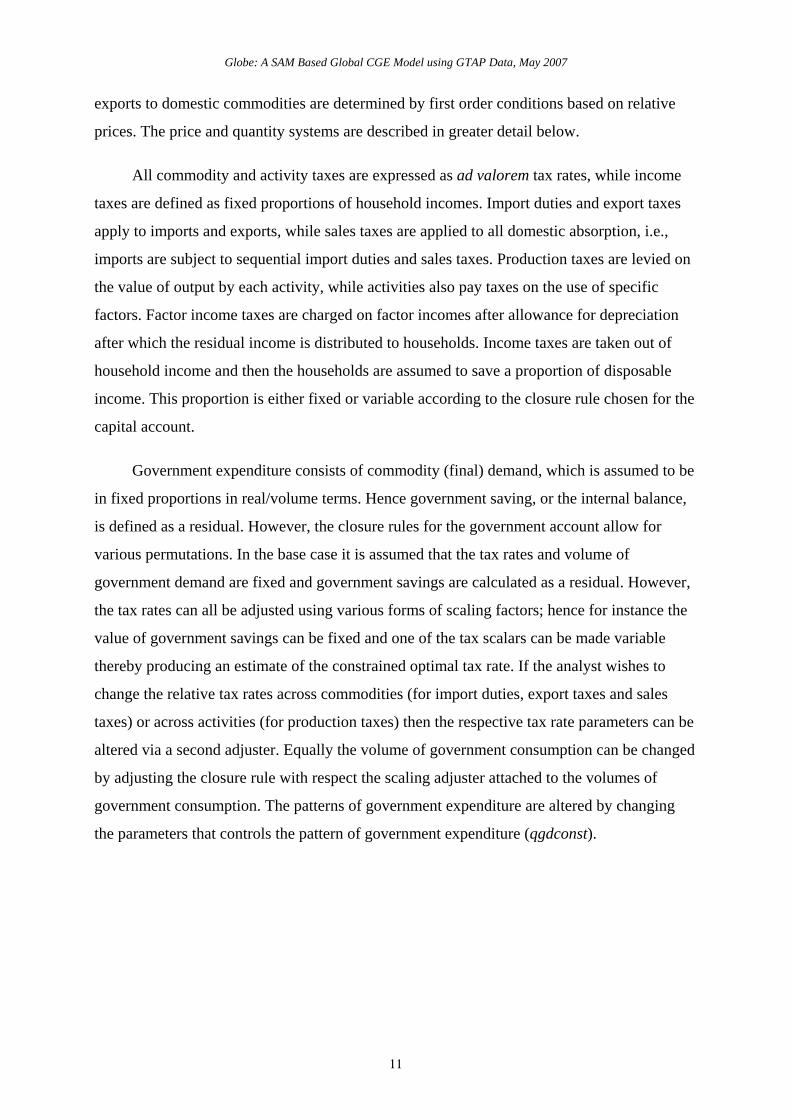
Government expenditure consists of commodity (final) demand, which is assumed to be

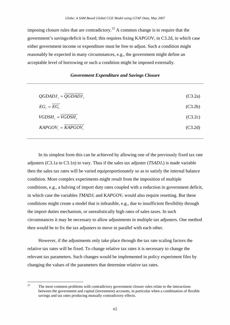
in fixed proportions in real/volume terms. Hence government saving, or the internal balance,

is defined as a residual. However, the closure rules for the government account allow for

various permutations. In the base case it is assumed that the tax rates and volume of

government demand are fixed and government savings are calculated as a residual. However,

the tax rates can all be adjusted using various forms of scaling factors; hence for instance the

value of government savings can be fixed and one of the tax scalars can be made variable

thereby producing an estimate of the constrained optimal tax rate. If the analyst wishes to

change the relative tax rates across commodities (for import duties, export taxes and sales

taxes) or across activities (for production taxes) then the respective tax rate parameters can be

altered via a second adjuster. Equally the volume of government consumption can be changed

by adjusting the closure rule with respect the scaling adjuster attached to the volumes of

government consumption. The patterns of government expenditure are altered by changing

the parameters that controls the pattern of government expenditure (qgdconst).


12

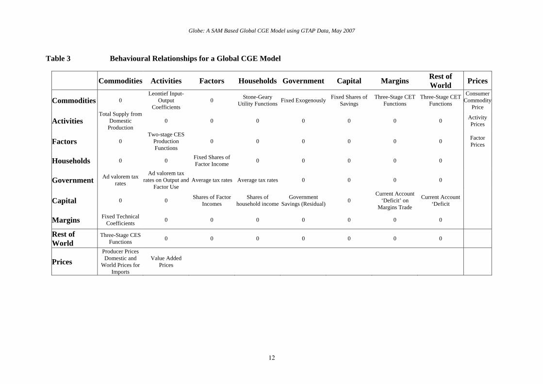
Table 3 Behavioural Relationships for a Global CGE Model

Commodities Activities Factors Households Government Capital Margins Rest of World Prices

Commodities 0 Leontief Input-

Output Coefficients

0 Stone-Geary Utility Functions Fixed Exogenously Fixed Shares of

Savings Three-Stage CET

Functions Three-Stage CET

Functions

Consumer Commodity

Price

Activities Total Supply from

Domestic Production

0 0 0 0 0 0 0 Activity Prices

Factors 0 Two-stage CES

Production Functions

0 0 0 0 0 0 Factor Prices

Households 0 0 Fixed Shares of Factor Income 0 0 0 0 0

Government Ad valorem tax rates

Ad valorem tax rates on Output and

Factor Use Average tax rates Average tax rates 0 0 0 0

Capital 0 0 Shares of Factor Incomes

Shares of household income

Government Savings (Residual) 0

Current Account ‘Deficit’ on

Margins Trade

Current Account ‘Deficit

Margins Fixed Technical Coefficients 0 0 0 0 0 0 0

Rest of World

Three-Stage CES Functions 0 0 0 0 0 0 0

Prices Producer Prices Domestic and

World Prices for Imports

Value Added Prices


13

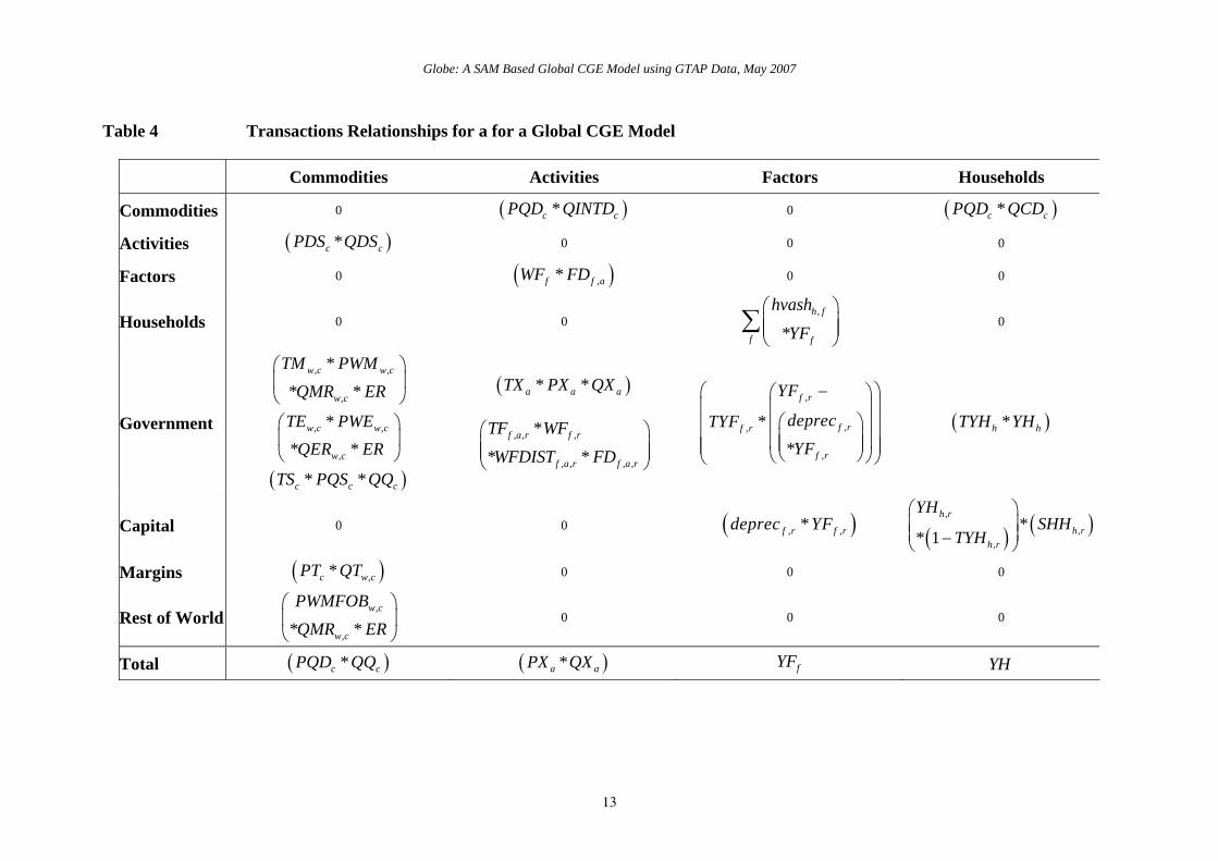
Table 4 Transactions Relationships for a for a Global CGE Model

Commodities Activities Factors Households

Commodities 0 ( )*c cPQD QINTD 0 ( )*c cPQD QCD

Activities ( )*c cPDS QDS 0 0 0

Factors 0 ( ),*f f aWF FD 0 0

Households 0 0 ,

*h f

f f

hvash

YF⎛ ⎞⎜ ⎟⎜ ⎟⎝ ⎠

∑ 0

Government

, ,

,

** *

w c w c

w c

TM PWMQMR ER

⎛ ⎞⎜ ⎟⎝ ⎠

, ,

,

** *

w c w c

w c

TE PWEQER ER

⎛ ⎞⎜ ⎟⎝ ⎠

( )* *c c cTS PQS QQ

( )* *a a aTX PX QX

, , ,

, , , ,

*

* *f a r f r

f a r f a r

TF WF

WFDIST FD⎛ ⎞⎜ ⎟⎜ ⎟⎝ ⎠

,

,,

,

**

f r

f rf r

f r

YF

deprecTYFYF

−⎛ ⎞⎛ ⎞⎜ ⎟⎜ ⎟

⎛ ⎞⎜ ⎟⎜ ⎟⎜ ⎟⎜ ⎟⎜ ⎟⎜ ⎟⎜ ⎟⎝ ⎠⎝ ⎠⎝ ⎠

( )*h hTYH YH

Capital 0 0 ( ), ,*f r f rdeprec YF ( ) ( ),

,,

** 1

h r

h rh r

YHSHH

TYH

⎛ ⎞⎜ ⎟⎜ ⎟−⎝ ⎠

Margins ( ),*c w cPT QT 0 0 0

Rest of World,

,* *w c

w c

PWMFOBQMR ER

⎛ ⎞⎜ ⎟⎝ ⎠

0 0 0

Total ( )*c cPQD QQ ( )*a aPX QX fYF YH


14

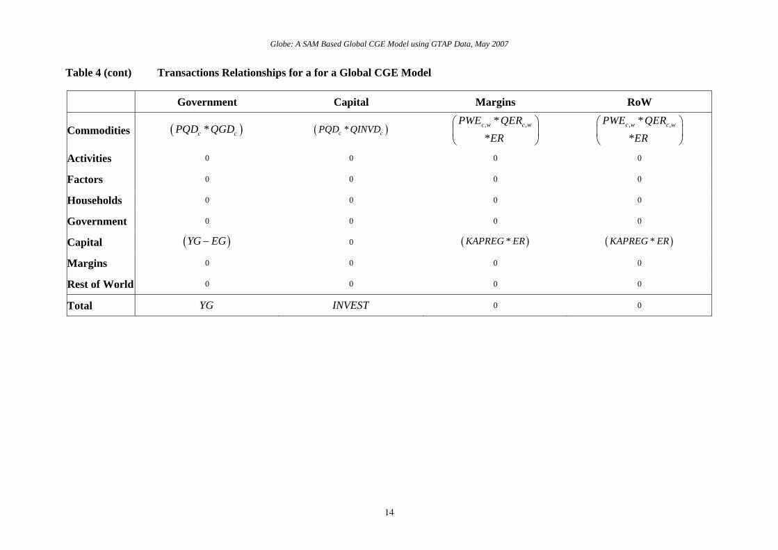
Table 4 (cont) Transactions Relationships for a for a Global CGE Model

Government Capital Margins RoW

Commodities ( )*c cPQD QGD ( )*c cPQD QINVD , ,**

c w c wPWE QERER

⎛ ⎞⎜ ⎟⎝ ⎠

, ,**

c w c wPWE QERER

⎛ ⎞⎜ ⎟⎝ ⎠

Activities 0 0 0 0

Factors 0 0 0 0

Households 0 0 0 0

Government 0 0 0 0

Capital ( )YG EG− 0 ( )*KAPREG ER ( )*KAPREG ER

Margins 0 0 0 0

Rest of World 0 0 0 0

Total YG INVEST 0 0


15

Total savings come from the households, the internal balance on the government

account and the external balance on the trade account. The external balance is defined as the

difference between the value of total exports and total imports, converted into domestic

currency units using the exchange rate. In the base model it is assumed that the exchange rates

are flexible and hence that the external balances are fixed. Alternatively the exchange rates

can be fixed and the external balances can be allowed to vary. Expenditures by the capital

account consist solely of commodity demand for investment. In the base solution it is

assumed that the shares of investment in total domestic final demand are fixed and that

household savings rates adjust so that total expenditures on investment are equal to total

savings, i.e., the closure rule presumes that savings are determined by the level of investment

expenditures. The patterns of investment volume are fixed, and hence the volume of each

commodity changes equiproportionately according to the total values of domestic final

demand. It is possible to fix the volumes of real investment and then allow the savings rates,

by households, to vary to maintain balances in the capital account, and it is possible to change

the patterns of investment by changing the investment parameters (qinvdconst).

Price and Quantity Systems for a Representative Region

Price System

The price system is built up using the principle that the components of the ‘price definitions’

for each region are the entries in the columns of the SAM. Hence there are a series of explicit

accounting identities that define the relationships between the prices and thereby determine

the processes used to calibrate the tax rates for the base solution. However, the model is set

up using a series of linear homogeneous relationships and hence is only defined in terms of

relative prices. Consequently as part of the calibration process it is necessary set some of the

prices equal to one (or any other number that suits the modeler) – this model adopts the

convention that prices are normalised at the level of the CES and CET aggregator functions

PQS, the supply price of the domestic composite consumption commodity and PXC, the

producer price of the composite domestic output. The price system for a typical region in a 4-

region global model is illustrated by Figure 1 – note that this representation abstracts from the

Globe region.

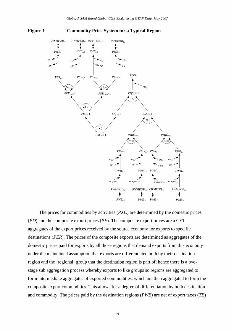
The relationships between the various prices in the model are illustrated in Figure 1.

The domestic consumer prices (PQD) are determined by the domestic prices of the


16

domestically supplied commodities (PD) and the domestic prices of the composite imports

(PM), and by the sales taxes (TS) that are levied on all domestic demand. The prices of the

composite imports are determined as aggregates of the domestic prices paid for imports from

all those regions that supply imports to this economy (PMR) under the maintained assumption

that imports are differentiated both by their source region and the ‘regional’ group that the

source region is part of; hence there is a two-stage sub aggregation process whereby imports

from like groups so regions are aggregated to form intermediate aggregates of imported

commodities, which are then aggregated to form the composite import commodities. This

allows for a degree of differentiation by both source and commodity.7 The region specific

import prices are expressed in terms of the domestic currency units after paying for trade and

transport services and any import duties. Thus a destination region is assumed to purchase a

commodity in a source economy where the price is defined in “world dollars” at the basket

exchange rate and is valued free on board (fob), i.e., PWMFOB. The carriage insurance and

freight (cif) price (PWM) is then defined as the fob price plus trade and transport margin

services (margcor) times the unit price of margin services (PT). The cif prices are related to

the domestic price of imports by the addition of any import duties (TM) and then converted

into domestic currency units using the nominal exchange rate (ER).

7 The impact of an additional level of nesting is explored in McDonald and Thierfelder (2006).


17

Figure 1 Commodity Price System for a Typical Region

c

c

c,2

c,2

PEc = 1 PDc = 1 PMc = 1

PQSc = 1

PXCc = 1

tsc

PQDc

tm1,c

ER

margcor1,c

tec,1

ER

tec,3

ER

tec,2

ER

PERc,wm=1 PERc,wm=1

PWEc,1 PWEc,3PWEc,2

PWMFOB1,c PWMFOB3,cPWMFOB2,c

PERc,1 PERc,2 PERc,3 PERc,4

tec,4

ER

PWEc,4

PWMFOB4,c

PMRwm,c PMRwm,c

PWM1,c PWM4,cPWM2,c

tm2,c

ER

tm4,c

ER

margcor4,cmargcor2,c

PWEc,1 PWEc,4PWEc,2

PWMFOB1,c PWMFOB4,cPWMFOB2,c

PMR1,c PMR2,c PMR3,c PMR4,c

PWM3,c

tm3,c

ER

margcor3,c

PWEc,3

PWMFOB3,c

c,31 c,32

c,32c,31

The prices for commodities by activities (PXC) are determined by the domestic prices

(PD) and the composite export prices (PE). The composite export prices are a CET

aggregates of the export prices received by the source economy for exports to specific

destinations (PER). The prices of the composite exports are determined as aggregates of the

domestic prices paid for exports by all those regions that demand exports from this economy

under the maintained assumption that exports are differentiated both by their destination

region and the ‘regional’ group that the destination region is part of; hence there is a two-

stage sub aggregation process whereby exports to like groups so regions are aggregated to

form intermediate aggregates of exported commodities, which are then aggregated to form the

composite export commodities. This allows for a degree of differentiation by both destination

and commodity. The prices paid by the destination regions (PWE) are net of export taxes (TE)


18

and are expressed in the currency units of the model’s reference region by use of the nominal

exchange. Notice how the export prices by region of destination (PER), and the intermediate

aggregates, are all normalised on 1, but the seeming counterpart of normalising import prices

by source region (PMR) are not normalised on 1. The link between the regions is therefore

embedded in the identification of the quantities exchanged rather than the normalised prices

and is a natural consequence of the normalisation process. The CET function can be switched

off so that the domestic and export commodities are assumed to be perfect substitutes; this is

the assumption in the GTAP model and is an option in this model.

The price system also contains a series of equilibrium identities. Namely the fob export

price (PWE) for region x on its exports to region y must be identical to the fob import price

(PWMFOB) paid by region y on its imports from region x. These equilibrium identities are

indicated by double headed arrows.

Quantity System

The quantity system for a representative region is somewhat simpler (see Figure 2). The

composite consumption commodity (QQ) is a mix of the domestically produced commodity

(QD) and the composite import commodity (QM), where the domestic and imported

commodities are imperfect substitutes, and the import commodities are differentiated both by

their source region and the ‘regional’ group that the source region is part of; hence there is a

two-stage sub aggregation process whereby imports from like groups so regions are

aggregated to form intermediate aggregates of imported commodities, which are then

aggregated to form the composite import commodities. The equilibrium conditions require

that the quantities imported from different regions (QMR) are identical to the quantities

exported by other regions to the representative region (QER). The composite consumption

commodity is then allocated between domestic intermediate demands (QINTD), private

consumption demand (QCD), government demand (QGD) and investment demand (QINVD).


19

Figure 2 Quantity System for a Typical Region

On the output side, domestic output by activity (QX) is identical to domestic commodity

output (QXC). Domestically produced commodities are then allocated between the domestic

market (QD) and composite export commodities (QE) under the maintained assumption of

imperfect transformation. Exports are differentiated both by their destination region and the

‘regional’ group that the destination region is part of; hence there is a two-stage sub

aggregation process whereby exports to like groups so regions are aggregated to form

intermediate aggregates of exported commodities, which are then aggregated to form the

composite export commodities.

Production System

The production system is set up as a two-stage nest of CES production functions (see Figure

3). At the top level aggregate intermediate inputs (QINT) are combined with aggregate

primary inputs (QVA) to produce the output of an activity (QX). This top level production

function can take either CES or Leontief form, with CES being the default and the elasticities

being activity and region specific.8 Aggregate intermediate inputs are a Leontief aggregation

of the individual intermediate inputs where the input-output coefficients (ioqint) are defined

in terms of input quantities relative to the aggregate intermediate input. The value added

8 The model allows the user to specify the share of intermediate input cost in total cost below which the

Leontief alternative is automatically selected.


20

production function is a standard CES function over all primary inputs, with the elasticities

being activity and region specific. The operation of this aggregator function can, of course, be

influenced by choices over the closure rules for the factor accounts.

Figure 3 Production Quantity System for a Typical Region

In the price system for production (see Figure 4) the value added prices (PVA) are

determined by the activity prices (PX), the production tax rates (TX), the input-output

coefficients (ioqint) and the commodity prices (PQD). The activity prices are a one to one

mapping of the commodity prices received by activities (PXC); this is a consequence of the

supply matrix being a square diagonal matrix.

Figure 4 Production Price System for a Typical Region


21

The Globe Region

An important feature of the model is the use of the concept of a region known as Globe.

While the GTAP database contains complete bilateral information relating to the trade in

commodities, i.e., in all cases transactions are identified according to their region of origin

and their region of destination, this is not the case for trade in margins services associated

with the transportation of commodities. Rather the GTAP database identifies the demand, in

value terms, for margin services associated with imports by all regions from all other regions

but does not identify the region that supplies the margin services associated with any specific

transaction. Consequently the data for the demand side for margin services is relatively

detailed but the supply side is not. Indeed the only supply side information is the total value

of exports of margin services by each region. The Globe construct allows the model to get

around this shortage of information, while simultaneously providing a general method for

dealing with any other transactions data where full bilateral information is missing.

The price system for the Globe region is illustrated in Figure 5. On the import side

Globe operates like all other regions. The commodities used in trade and transport services

are assumed to be differentiated by source region and ‘regional’ group and aggregated using a

two-level CES function and can potentially incur trade and transport margins (margcor) and

face tariffs (TM); in fact the database does not include any transport margins or tariff data for

margin services in relation to the destination region, although they can, and do, incur export

taxes levied by the exporting region.


22

Figure 5 Price System for the Globe Region

∞

The export side is slightly different. In effect the Globe region is operating as a method

for pooling differentiated commodities used in trade and transport services and the only

differences in the use of trade and transport services associated with any specific import are

the quantities of each type of trade service used and the mix of types of trade services.

Underlying this is the implicit assumption that each type of trade service is homogenous, and

should be sold therefore at the same price. Hence the export price system for Globe needs to


23

be arranged so that Globe exports at a single price, i.e., there should be an infinite elasticity of

substitution between each type of trade service exported irrespective of its destination region.

Therefore the average export price (PE) should equal the price paid by each destination

region (PER), which should equal the export price in world currency units (PWE) and will be

common across all destinations (PT).

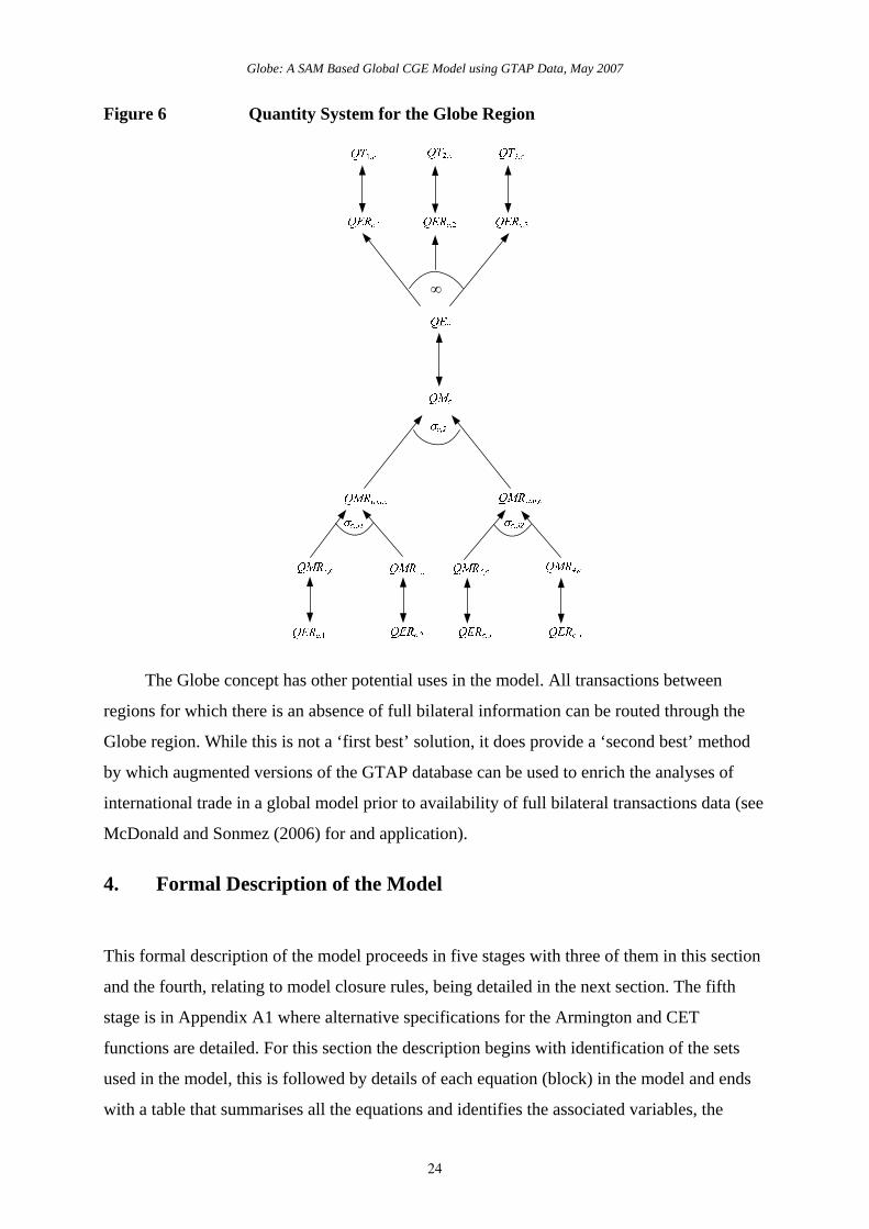
The linked quantity system contains the same asymmetry in the treatment of imports

and exports by Globe (see Figure 6). The imports of trade and transport commodities are

assumed to be differentiated by region and ‘regional’ group of origin, hence the elasticity of

substitution is greater than zero but less than infinity, while the exports of trade and transport

commodities are assumed to be homogenous and hence the elasticities of transformation are

infinite.

One consequence of using a Globe region for trade and transport services is that Globe

runs trade balances with all other regions. These trade balances relate to the differences in the

values of trade and transport commodities imported from Globe and the value of trade and

transport commodities exported to Globe; however the sum of Globe’s trade balances with

other regions must be zero since Globe is an artificial construct rather than a real region. But

the demand for trade and transport services by any region is determined by technology, i.e.,

the coefficients margcor, and the volume of imports demanded by the destination region. This

means that the prices of trade and transport commodities only have an indirect effect upon

their demand – the only place these prices enter into the import decision as a variable is as a

partial determinant of the difference between the fob and cif valuations of other imported

commodities. Consequently the primary market clearing mechanism for the Globe region

comes through the quantity of trade and transport commodities it chooses to import.


24

Figure 6 Quantity System for the Globe Region

∞

The Globe concept has other potential uses in the model. All transactions between

regions for which there is an absence of full bilateral information can be routed through the

Globe region. While this is not a ‘first best’ solution, it does provide a ‘second best’ method

by which augmented versions of the GTAP database can be used to enrich the analyses of

international trade in a global model prior to availability of full bilateral transactions data (see

McDonald and Sonmez (2006) for and application).

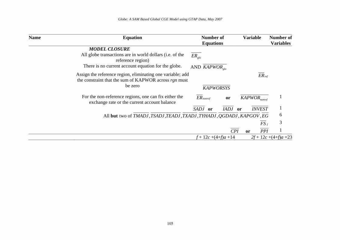
4. Formal Description of the Model

This formal description of the model proceeds in five stages with three of them in this section

and the fourth, relating to model closure rules, being detailed in the next section. The fifth

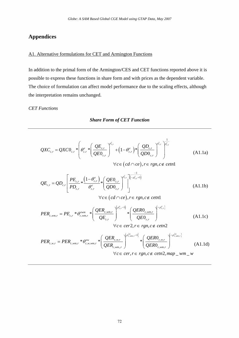
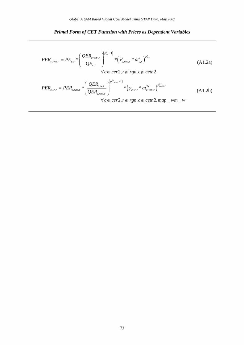
stage is in Appendix A1 where alternative specifications for the Armington and CET

functions are detailed. For this section the description begins with identification of the sets

used in the model, this is followed by details of each equation (block) in the model and ends

with a table that summarises all the equations and identifies the associated variables, the


25

counts for equations and variables and identifies whether the equation is implemented or not

for the Globe region.

Model Sets

Rather than writing out each and every equation in detail it is useful to start by defining a

series of sets; thereafter if a behavioural relationship applies to all members of a set an

equation only needs to be specified once. The natural choice for this model is a set for all the

transactions by each region (sac) plus a series of sets that group commodities, activities,

factors, import duties, export taxes, trade margins, trade and finally some individual accounts

relating to domestic institutions. The outer set for any region is defined as

{ }, , , , , , , , , , ,sac c a f h tmr ter tff g i owatpmarg ww total=

and the following are the basic sets for each region in this model

{ }{ }{ }

( ) { }{ }{ }{ }

( ) { }( ) { }

( ) commodities

( ) activities

( ) factors

households

( ) import duties

( ) export taxes

( ) factort taxes

saltax, prodtax, factax, dirtax, Govt

kap

( ) trade

c sac

a sac

f sac

h sac

tmr sac

ter sac

tff sac

g sac

i sac

owatpmarg sac

=

=

=

=

=

=

=

=

=

= { }{ }{ }{ }

and transport margins

( ) rest of the world - trade partners and aggregates

( ) rest of the world - aggregates

( ) rest of the world - trade partners

ww sac

wm ww

w ww

=

=

=

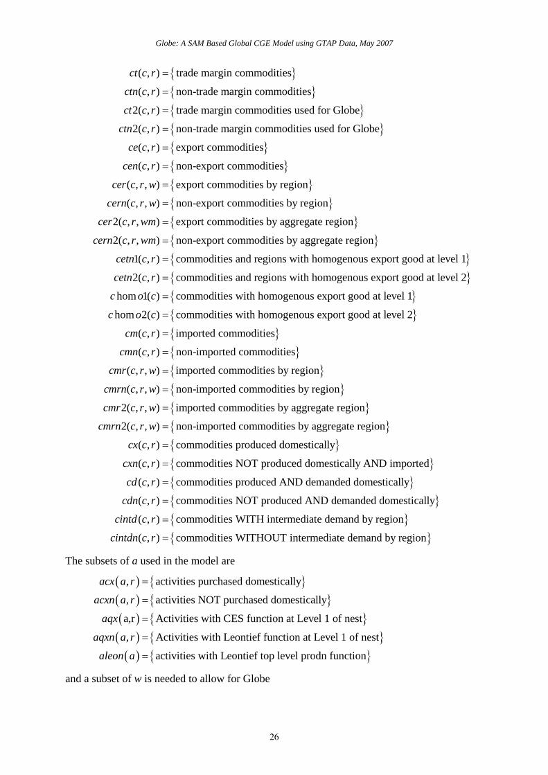
Various subsets of c are declared and then assigned on the basis of certain

characteristics of the data set used to calibrate the specific implementation of the model, so-

called dynamic sets. These subsets of c used in this model are


26

{ }{ }{ }{ }{ }

( , ) trade margin commodities

( , ) non-trade margin commodities

2( , ) trade margin commodities used for Globe

2( , ) non-trade margin commodities used for Globe

( , ) export commodities

(

ct c r

ctn c r

ct c r

ctn c r

ce c r

cen

=

=

=

=

=

{ }{ }{ }{ }

, ) non-export commodities

( , , ) export commodities by region

( , , ) non-export commodities by region

2( , , ) export commodities by aggregate region

2( , , ) non-export commodities by

c r

cer c r w

cern c r w

cer c r wm

cern c r wm

=

=

=

=

= { }{ }{ }

aggregate region

1( , ) commodities and regions with homogenous export good at level 1

2( , ) commodities and regions with homogenous export good at level 2

hom 1( ) commodities with homogenous

cetn c r

cetn c r

c o c

=

=

= { }{ }{ }{ }{ }

export good at level 1

hom 2( ) commodities with homogenous export good at level 2

( , ) imported commodities

( , ) non-imported commodities

( , , ) imported commodities by region

( , , ) non

c o c

cm c r

cmn c r

cmr c r w

cmrn c r w

=

=

=

=

= { }{ }{ }{ }

-imported commodities by region

2( , , ) imported commodities by aggregate region

2( , , ) non-imported commodities by aggregate region

( , ) commodities produced domestically

( , ) commoditie

cmr c r w

cmrn c r w

cx c r

cxn c r

=

=

=

= { }{ }{ }

s NOT produced domestically AND imported

( , ) commodities produced AND demanded domestically

( , ) commodities NOT produced AND demanded domestically

( , ) commodities WITH intermediate demand

cd c r

cdn c r

cintd c r

=

=

= { }{ }

by region

( , ) commodities WITHOUT intermediate demand by regioncintdn c r =

The subsets of a used in the model are

( ) { }( ) { }( ) { }

( ) { }

, activities purchased domestically

, activities NOT purchased domestically

a,r Activities with CES function at Level 1 of nest

, Activities with Leontief function at Level 1 of nest

acx a r

acxn a r

aqx

aqxn a r

a

=

=

=

=

( ) { }activities with Leontief top level prodn functionleon a =

and a subset of w is needed to allow for Globe


27

( ) { }Rest of world without Globewgn w = .

It is also necessary to define a set of regions, r, for which there are two subsets

{ }{ }{ }{ }

( ) all regions excluding Globe

( ) reference regions for global numeraire

( ) regions with Leontief top level prodn function

hom 1( ) regions with homogenous export good at level 1

hom 2( )

rgn r

ref r

rleon r

r o c

r o c

=

=

=

=

= { }regions with homogenous export good at level 2

.

A macro SAM that facilitates checking various aspects of model calibration and

operation is used in the model and this needs another set, ss,

, , , ,, , , , ,

commdty activity valuad hholdsss

tmtax tetax govtn kapital margs,world totals⎧ ⎫

= ⎨ ⎬⎩ ⎭

.

The model also makes use of a series of mapping files that are used to link sets. These

are

( ) { }( ) { }( ) { }( ) { }

{ }

_ _ , Tariff mapping

_ _ , Tariff mapping reverse

_ _ , Export tax mapping

_ _ , Export tax mapping reverse

_ _ ( , ) trade partner to aggregate region mapping

_

map w tmr w tmr

map tmr w tmr w

map w ter w ter

map ter w ter w

map wm w wm w

map

=

=

=

=

=

( ) { }( ) { }

( ) { }( )

_ _ , , Trade margin mapping of owatpmarg to ct2 and w

_ _ , Trade margin mapping of w to owatpmarg

_ , Region to trade partner mapping

_ , Region to trade partn

c w marg c w owatpmarg

map marg w owatpmarg w

mapr w r w

mapw r w r

=

=

=

= { }( ) { }

( ) { }

er mapping

_ _ , Factor taxes to factors

_ _ , Factor taxes to factors reverse

map f tff f tff

map tff f tff ff

=

=

Finally various other sets are declared to facilitate model operation. These are


28

( ) { }( ) { }

{ }

SAM accounts without totals

Macro SAM accounts without totals

set for programme control parameters

SACN sac

ssn ss

cons

=

=

=

Reserved Names

The model uses a number of names that are reserved; these are

DIRTAX Direct TaxesSALTAX Sales Taxes

PRODTAX Production TaxesFACTAX Factor Taxes

.

Conventions

The equations for the model are set out in 9 ‘blocks’ each of which can contain a number of

sub blocks. The equations are grouped under the following headings:

1. TRADE BLOCK

a. Exports Block

b. Imports Block

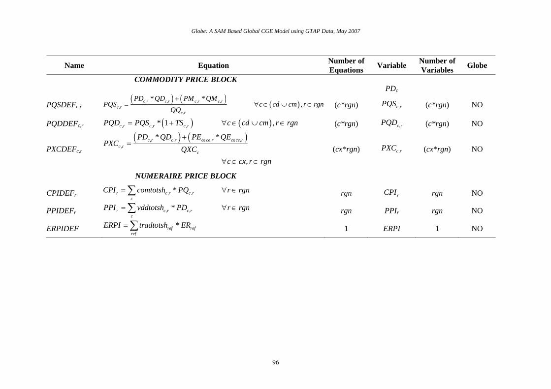
2. COMMODITY PRICE BLOCK

3. NUMERAIRE PRICE BLOCK

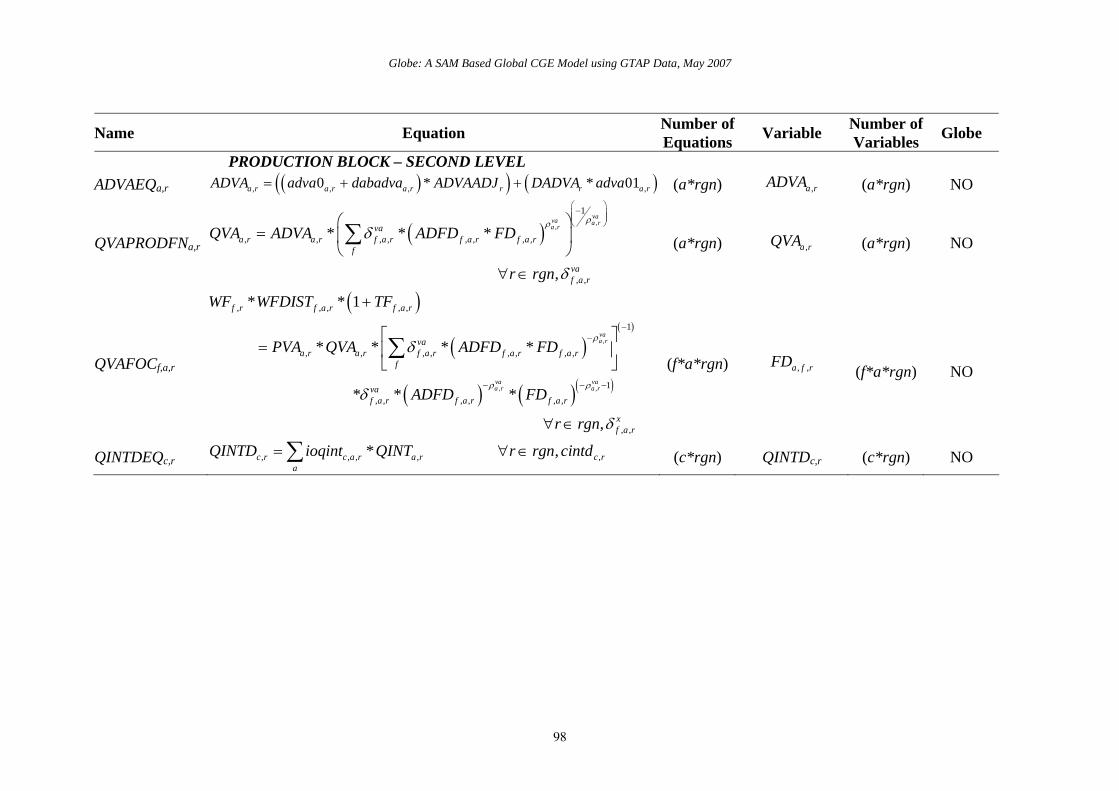
4. PRODUCTION BLOCK

a. Production

b. Intermediate Input Demand

c. Commodity Output

d. Activity Output

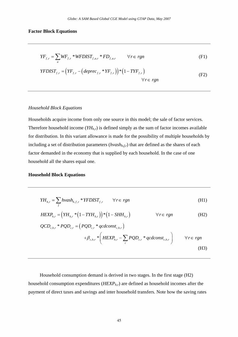
5. FACTOR BLOCK

6. HOUSEHOLD BLOCK

a. Household Income

b. Household Expenditure

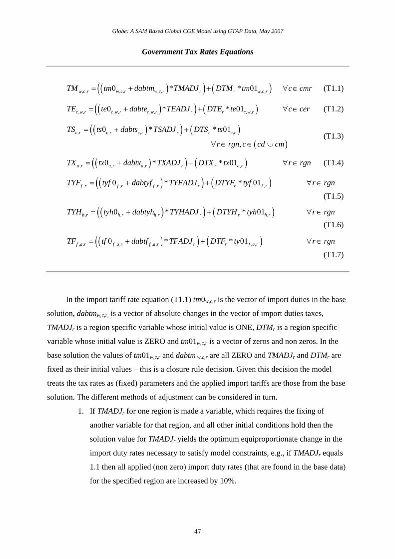
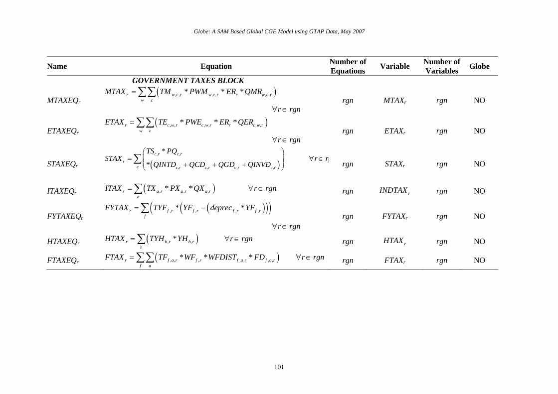
7. GOVERNMENT BLOCK

a. Government Tax Rates

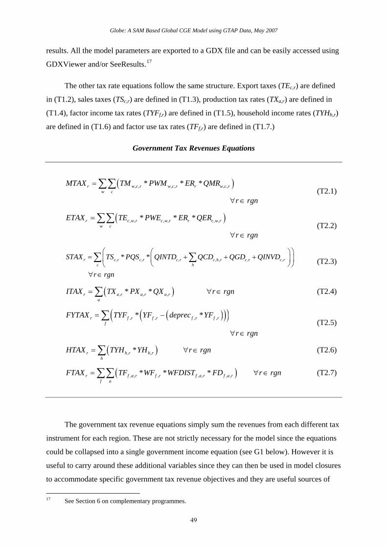
b. Government Tax Revenues

c. Government Income

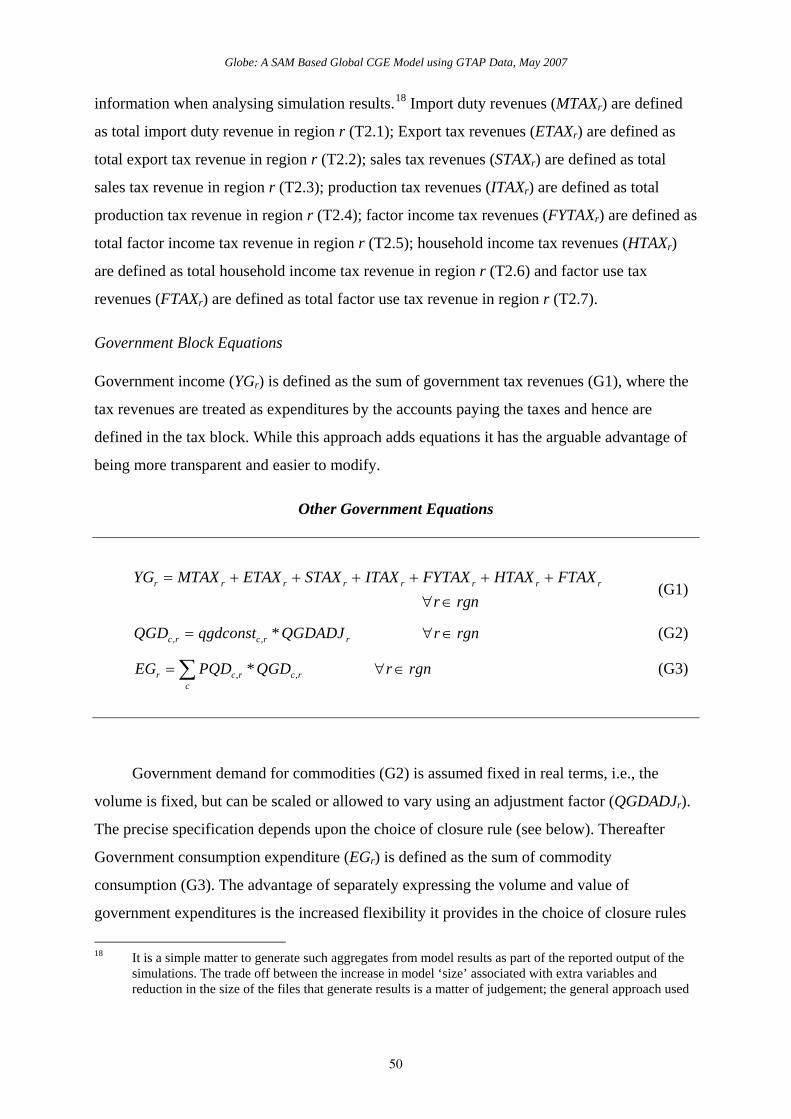
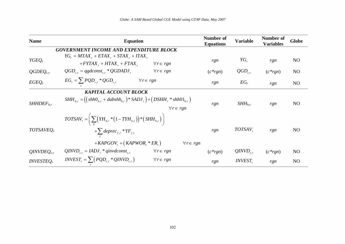
d. Government Expenditure Block


29

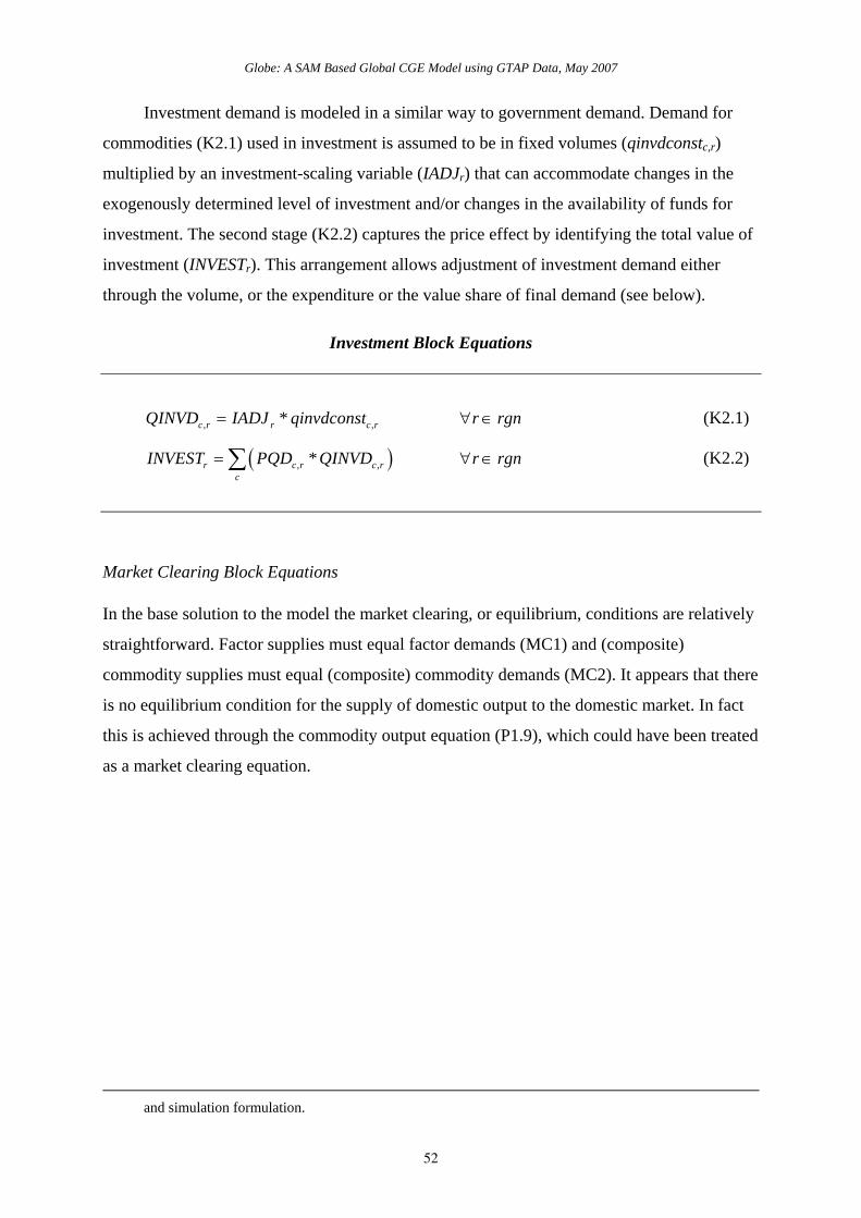
8. KAPITAL BLOCK

a. Savings Block

b. Investment Block

9. MARKET CLEARING BLOCK

a. Factor Accounts

b. Commodity Accounts

c. Investment and Savings Accounts

d. Commodity Trade Accounts

e. Margin Trade Accounts

f. Absorption Closure

g. Slack

This grouping is carried throughout the model code, i.e., it is followed for the parameter

declaration and calibration, variable declaration and variable initialization sections. This

modularization of the code is adopted for ease of reading and altering the model rather than

being a requirement of the model.

A series of conventions are adopted for the naming of variables and parameters. These

conventions are not a requirement of the modeling language; rather they are designed to ease

reading of the model.

All VARIABLES are in upper case.

The standard prefixes for variable names are: P for price variables, Q for quantity

variables, W for factor prices, F for factor quantities, E for expenditure variables, Y

for income variables, and V for value variables

All variables have a matching parameter that identifies the value of the variable in

the base period. These parameters are in upper case and carry a ‘0’ suffix, and are

used to initialise variables.

A series of variables are declared that allow for the equiproportionate multiplicative

adjustment of groups of variables. These variables are named using the convention

**ADJ, where ** is the variable series they adjust.

A series of variables are declared that allow for the additive adjustment of groups of

variables. These variables are named using the convention D**, where ** is the

variable series they adjust.


30

All parameters are in lower case, except those paired to variables that are used to

initialise variables.

Parameter names have a two or five character suffix which distinguishes their

definition, e.g., **sh is a share parameter, **av is an average and **const is a

constant parameter.

For the Armington (CES) functions all the share parameters are declared with the

form delta**, all the shift/efficiency parameters are declared with the form ac**,

and all the elasticity parameters are declared with the form rho**, where **

identifies the function in which the parameter operates.

For the CET functions all the share parameters are declared with the form

gamma**, all the shift/efficiency parameters are declared with the form at**, and all

the elasticity parameters are declared with the form rho**, where ** identifies the

function in which the parameter operates.

All coefficients in the model are declared with the form io****, where **** consists

of two parts that identify the two variables related by the coefficient.

The index ordering follows the specification in the SAM: row, column, and then r to

indicate the region. For example, exports from region r to region w would be

QERc,w,r because region r’s export data in its SAM is found in the commodity row

(c) and the trade partner column (w). Likewise, imports in region r from region w

are designated, QMRw,c,r because region r’s import data in its SAM is found in the

trade partner row (w) and the commodity column (c).

All sets have another name, or alias, given by the set name followed by “p”. For

example, the set of commodities may be called c or cp.

Equations for the Model

The model equations are reported and described by blocks/groups below and then they are

summarised in table A4 in the appendix.

Exports Block Equations

The treatment of exports is complicated by the incorporation of the facility to treat export

commodities as imperfect or perfect substitutes for domestic commodities and by the need to

accommodate the special case of exports (of trade and transport services) that are

homogenous from Globe. The presumption of imperfect substitution is the default


31

presumption in this model; reasons for this decision being its symmetry with the Armington

assumption on the imports side, the amelioration of the terms of trade effects associated with

the Armington assumption and a belief that in general there is differentiation between

commodities supplied to domestic and export markets. However there are proponents of the

arguments for treating exports as perfect substitutes and there are clearly cases where such an

assumption may be appropriate, e.g., supplies of unprocessed mineral products.9 The

formulation of the model allows the CET functions to be switched off at either or both levels

of the export supply nest for specific commodities and/or for specific regions, via the sets

ccetn1 and ccetn2.

When exports and domestic commodities are defined as imperfect substitutes, the

domestic prices of commodity exports, c, by destination, w, and source, r, region (PERc,w,r)

are defined as the product of world prices of exports (PWEc,w,r) – also defined by commodity

and destination and source region, the source region’s exchange rate (ERr) and one minus the

export subsidy rate10 (TEc,w,r) (X3). The possibility of non-traded commodities means that the

equations for the domestic prices of exports are only implemented for those commodities that

are traded; this requires the use of a dynamic set, cer, which is defined by those commodities

that are exported in the base data. Also notice that the world prices of exports (PWEc,w,r) are

defined as variables; in a global model the small country trade assumption is not valid since,

by definition, world prices are endogenous and therefore ALL regions are treated as ‘large’

producers of a commodity.

Export Block Equations 1

9 The GTAP model assumes perfect substitution and historically it has been argued that perfect substitution

is appropriate for Australia. 10 Defining export taxes as negative subsidies means that there is symmetry between the treatment of import

duties and export subsidies when coding the model in GAMS.


32

, , , , , ,* * ,c r c r c wm r c wm rwm

PE QE PER QER c ce r rgn= ∀ ∈ ∈∑ (X1)

, , , , 1,c r c rPE PD c ce c cd c cetn r rgn= ∀ ∈ ∈ ∈ ∈ (X2)

( ), , , , , ,* * 1c w r c w r r c w rPER PWE ER TE c cer= − ∀ ∈ (X3)

( )( ) , , , ,$ _ _ ,, ,

, ,

*2,

c w r c w rw map wm w wm wc wm r

c wm r

PER QERPER c cer r rgn

QER= ∀ ∈ ∈

∑ (X4)

, , , 2, 2,c wm r c rPER PE c cer c cetn r rgn= ∀ ∈ ∈ ∈ (X5)

( ) ( ), , ,

2, , OR , , 2c w r c rPER PE

c ct r rgn w wgn c cer r rgn c cetn

=

∀ ∈ ∉ ∈ ∀ ∈ ∈ ∈ (X6)

The prices of the composite export commodities to aggregate regions (wm) can be

expressed as simple volume weighted averages of the export prices for regions assigned to

that aggregate, where PERc,wm,r and QERc,wm,r are the price and quantity of the composite

export commodity c from region r to the aggregate region wm (X4). This comes from the fact

that a CET function is linear homogeneous and hence Eulers theorem can be applied.

Likewise, the prices of the composite export commodities can then be expressed as simple

volume weighted averages of the of the export prices by region (X1), where PEc,r and QEc,r

the price and quantity of the composite export commodity c from region r, and the weights

are the volume shares of exports and are variable. Notice, however, that (X1) and (X4) are

only implemented of the set rgn, i.e. the region Globe, whose exports are always homogenous

goods, is excluded.

When exports are homogeneous, it may be that the aggregate export and domestic good

are imperfect substitutes but exports to partners are homogenous (i.e. perfect substitutes).

Alternatively, it may be that the aggregate export and domestic good are homogeneous and

therefore, necessarily, exports to all partners are homogeneous. When the aggregate export

and the domestic good are homogenous, the assignment is made in the set cetn1(c,r). When

exports to regions are homogenous, the assignment is made in set cetn2(c,r). Note that if a

commodity and region are assigned to set cetn1(c,r), they are automatically assigned to

cetn2(c,r). However, entries in cetn2(c,r) are not automatically assigned to the set cetn1(c,r).


33

Equations (X5) and (X6) define the price relationships when exports to partners are

homogenous—the price is the same to all export destinations. Equation (X5) controls level 2

and (X6) controls level 3. When exports and domestic commodities are perfect substitutes at

the top level of the export nest, then export and domestic prices equate (X2). Note that if

equation (X2) applies to a region and commodity, then equations (X5) and (X6) also apply

because all entries in the set ccetn1(c,r) are also in ccetn2(c,r).11

It is assumed that the margin commodities exported by Globe are perfect substitutes for

each other, i.e., the same price is paid for each trade margin commodity by ALL purchasing

regions. Equation (X6) is always selected for the composite export price for trade margin

commodities from Globe.


( )( )( )

, , ,

1

, , , , , ,. * 1 *

, , 1

t t tc r c r c r

c r c r c r c r c r c rQXC at QE QD

c cd ce r rgn c cetn

ρ ρ ργ γ= + −

∀ ∈ ∩ ∈ ∉ (X7)

( ) ( )

( )

,

11

,,, ,

, ,

1*

, , 1

tc rc rc r

c r c rc r c r

PEQE QD

PD


ργγ

−⎡ ⎤−= ⎢ ⎥

⎢ ⎥⎣ ⎦∀ ∈ ∩ ∈ ∉

(X8)

( )( )( )( )( )( )

, , , ,

OR ,

OR , , 1

c r c r c rQXC QD QE c cd cen r rgn

c cdn ce r rgn


= + ∀ ∈ ∩ ∈

∀ ∈ ∩ ∈

∀ ∈ ∩ ∈ ∈

(X9)

, , 2,c r c rQE QM c ct r rgn= ∀ ∈ ∉ (X10)

, , , 2,c r c w rw

QE QER c ct r rgn= ∀ ∈ ∉∑ (X11)

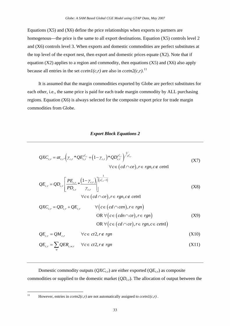
Domestic commodity outputs (QXCc,r) are either exported (QEc,r) as composite

commodities or supplied to the domestic market (QDc,r). The allocation of output between the

11 However, entries in ccetn2(c,r) are not automatically assigned to ccetn1(c,r) .


34

domestic and export markets is determined by the output transformation functions, Constant

Elasticity of Transformation (CET) functions, (X7) with the optimum ratio of QEc,r and QDc,r

determined by the ratio of first-order conditions (X8). In this version of the model the primal

form of the CET is used, although share forms exist (See Appendix A1). Some commodities

are produced solely for domestic sales or solely for export. In that case, equation (X9) is used.

If the domestic and aggregate export good are homogeneous, equation (X9) also applies.


( )

( ),

,

11

, ,, , ,

, , , ,

** *

2, , 2

ec r

ec r

c wm rc wm r c r

r rc r c wm r c r

PERQER QE

PE at

c cer r rgn c cetn

ρ

ργ

⎛ ⎞⎜ ⎟⎜ ⎟−⎝ ⎠⎛ ⎞

⎜ ⎟= ⎜ ⎟

⎛ ⎞⎜ ⎟⎜ ⎟⎜ ⎟⎝ ⎠⎝ ⎠∀ ∈ ∈ ∉

(X12)

( )

( )

( )

2, ,

2, ,

11

, ,, , , ,

2, , , , , ,

** *

, _ _ , , , 2

ec r wm

ec wm r

c w rc w r c wm r

r rc wm r c w r c wm r

PERQER QER

PER at

c cer map wm w wm w r rgn c cetn

ρ

ργ

⎛ ⎞⎜ ⎟⎜ ⎟−⎝ ⎠⎛ ⎞

⎜ ⎟= ⎜ ⎟

⎛ ⎞⎜ ⎟⎜ ⎟⎜ ⎟⎝ ⎠⎝ ⎠∀ ∈ ∈ ∉

(X13)

There is a need for an equilibrium conditions for trade by Globe. Since Globe is an

artificial construct whose sole role in the model is to gather exports whose destinations are

unknown and supply imports whose sources are unknown, and visa versa, it must always

balance its trade by commodity within each period. Thus the volume of exports of trade

margin commodities by Globe must be exactly equal to the volume imports of trade margin

commodities, see (X10). The export of trade margin commodities by Globe is covered by

(X11), which is a simple summation of quantities because the commodities are assumed to be

perfect substitutes.

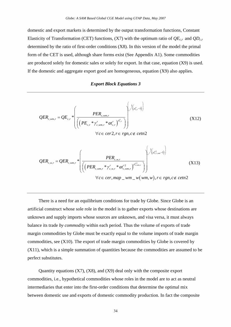
Quantity equations (X7), (X8), and (X9) deal only with the composite export

commodities, i.e., hypothetical commodities whose roles in the model are to act as neutral

intermediaries that enter into the first-order conditions that determine the optimal mix

between domestic use and exports of domestic commodity production. In fact the composite


35

export commodities are themselves CET aggregates of commodity exports to different

‘regional’ groups (QERc,wm,r) and different regions (QERc,w,r). The appropriate first order

conditions are given by (X12) for quantities exported to ‘regional’ groups and (X13) for

quantities exported to regions. Equations (X12) and (X13) are derived from the first-order

conditions for the optimal choice of export to the regional group (X12) or the regions(X13).12

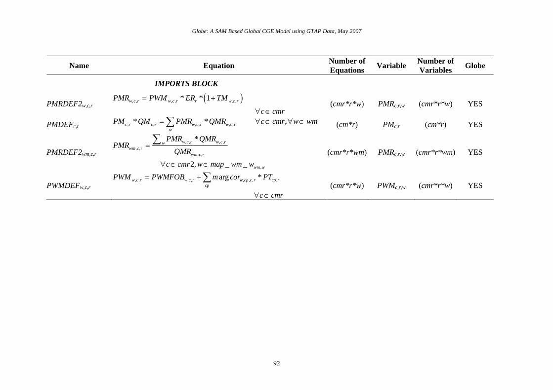
Imports Block Equations

The prices of imported commodities are made up of several components. The export price in

foreign currency units – valued free on board (fob) (PWMFOBw,c,r) – plus the cost of trade

and transport services, which gives the import price carriage insurance and freight (cif) paid

(PWMw,c,r), plus any import duties; all of which are then converted into domestic currency

units (PMRw,c,r). Clearly the import price values fob (PWMFOBw,c,r) are identical to the export

prices valued fob (PWEc,w,r) – this condition is imposed in the market clearing block (see

below) – and hence the cif price is defined in (M1), where margcorw,cp,c,r is the quantity of

trade and transport services (cp) required to import a unit of the imported commodity and

PTcp,r is the price of trade and transport services. Embedded in the definition of the coefficient

margcorw,cp,c,r is the explicit assumption that transporting a commodity from a specific source

to a specific destination requires the use of a specific quantity of services per unit imported–

the actual cost of these services can vary according to changes in the prices of the trade and

transport services or the quantity of services required to transport a particular commodity.

The domestic prices of imports from a region (PMRw,c,r) are then defined as the product

of world prices of imports (PWMw,c,r) – after payment for carriage, insurance and freight (cif)

- the exchange rate (ERr) and one plus the import tariff rate (TMw,c,r) (M2). The possibility of

non-traded commodities means that the equations for the domestic prices of imports are only

implemented for those commodities that are traded; this requires the use of a dynamic set,

cmr, which is defined by those commodities that are imported by a region from another region

in the base data.

The prices of the composite import commodities from ‘regional’ groups can be defined,

by exploiting Eulers theorem for linear homogenous functions, as the volume share weighted

sum the imports from those regions in each group (M3). Then the domestic prices can be

12 See Appendix A1 for a more conventional representation with prices on the left hand side.


36

expressed as simple volume weighted averages of the import prices by region, (M4) where

PMc,r and QMc,r are the price and quantity of the composite import commodity c by region r,

and the weights are the volume shares of imports and are variable. This comes from the fact

that a CES function is linear homogenous and hence Eulers theorem can be applied. Notice

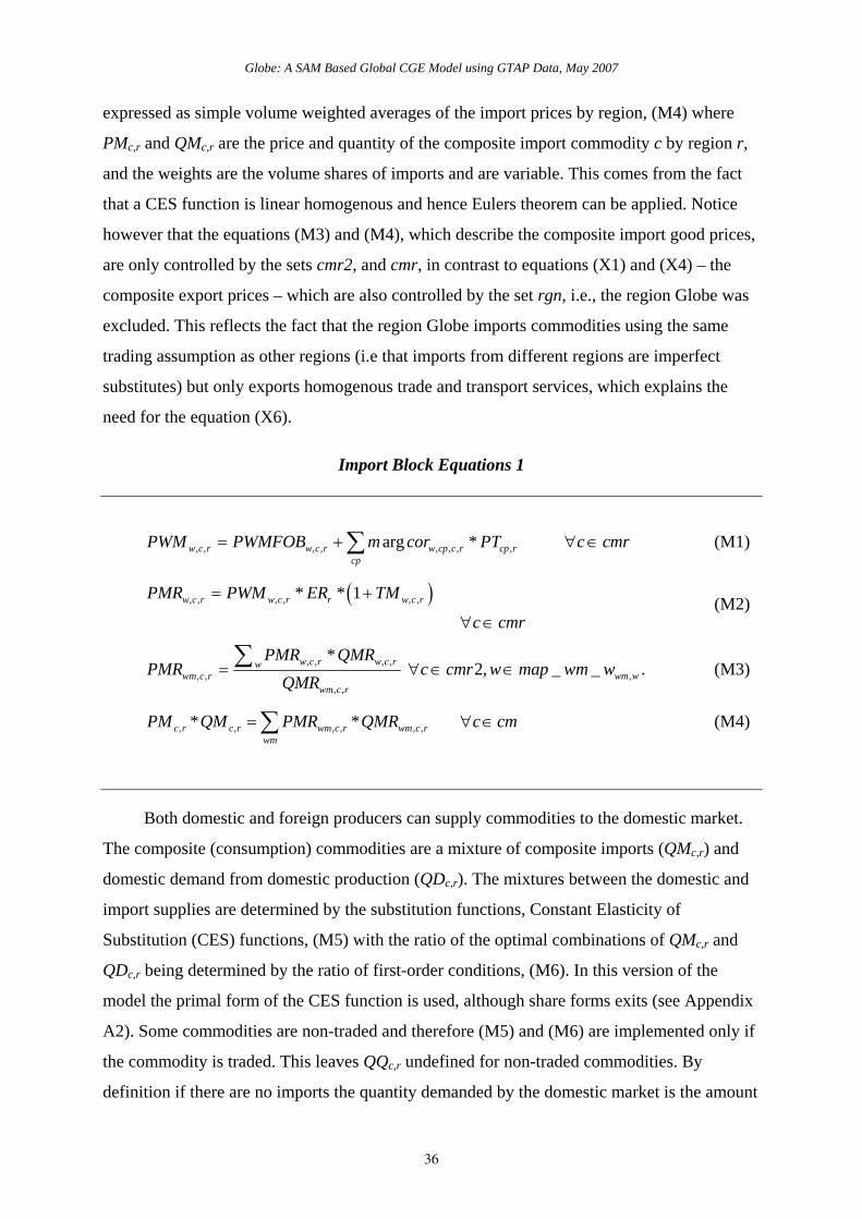
however that the equations (M3) and (M4), which describe the composite import good prices,

are only controlled by the sets cmr2, and cmr, in contrast to equations (X1) and (X4) – the

composite export prices – which are also controlled by the set rgn, i.e., the region Globe was

excluded. This reflects the fact that the region Globe imports commodities using the same

trading assumption as other regions (i.e that imports from different regions are imperfect

substitutes) but only exports homogenous trade and transport services, which explains the

need for the equation (X6).

Import Block Equations 1

, , , , , , , ,arg *w c r w c r w cp c r cp rcp

PWM PWMFOB m cor PT c cmr= + ∀ ∈∑ (M1)

( ), , , , , ,* * 1w c r w c r r w c rPMR PWM ER TM

c cmr

= +

∀ ∈ (M2)

, , , ,, , ,

, ,

*2, _ _w c r w c rw

wm c r wm wwm c r

PMR QMRPMR c cmr w map wm w

QMR= ∀ ∈ ∈∑ . (M3)

, , , , , ,* *c r c r wm c r wm c rwm

PM QM PMR QMR c cm= ∀ ∈∑ (M4)

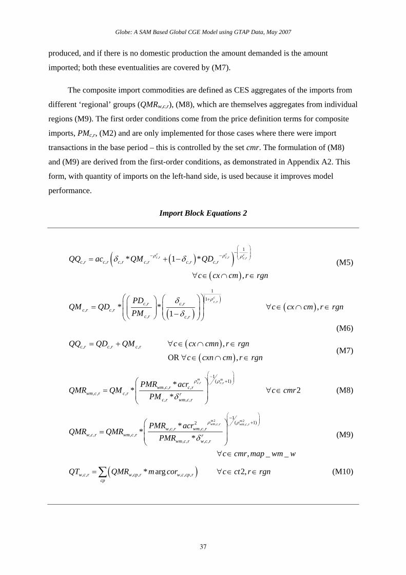
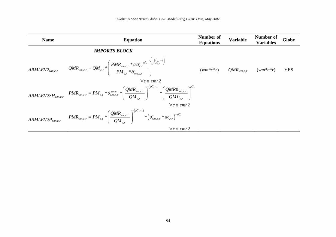
Both domestic and foreign producers can supply commodities to the domestic market.

The composite (consumption) commodities are a mixture of composite imports (QMc,r) and

domestic demand from domestic production (QDc,r). The mixtures between the domestic and

import supplies are determined by the substitution functions, Constant Elasticity of

Substitution (CES) functions, (M5) with the ratio of the optimal combinations of QMc,r and

QDc,r being determined by the ratio of first-order conditions, (M6). In this version of the

model the primal form of the CES function is used, although share forms exits (see Appendix

A2). Some commodities are non-traded and therefore (M5) and (M6) are implemented only if

the commodity is traded. This leaves QQc,r undefined for non-traded commodities. By

definition if there are no imports the quantity demanded by the domestic market is the amount


37

produced, and if there is no domestic production the amount demanded is the amount

imported; both these eventualities are covered by (M7).

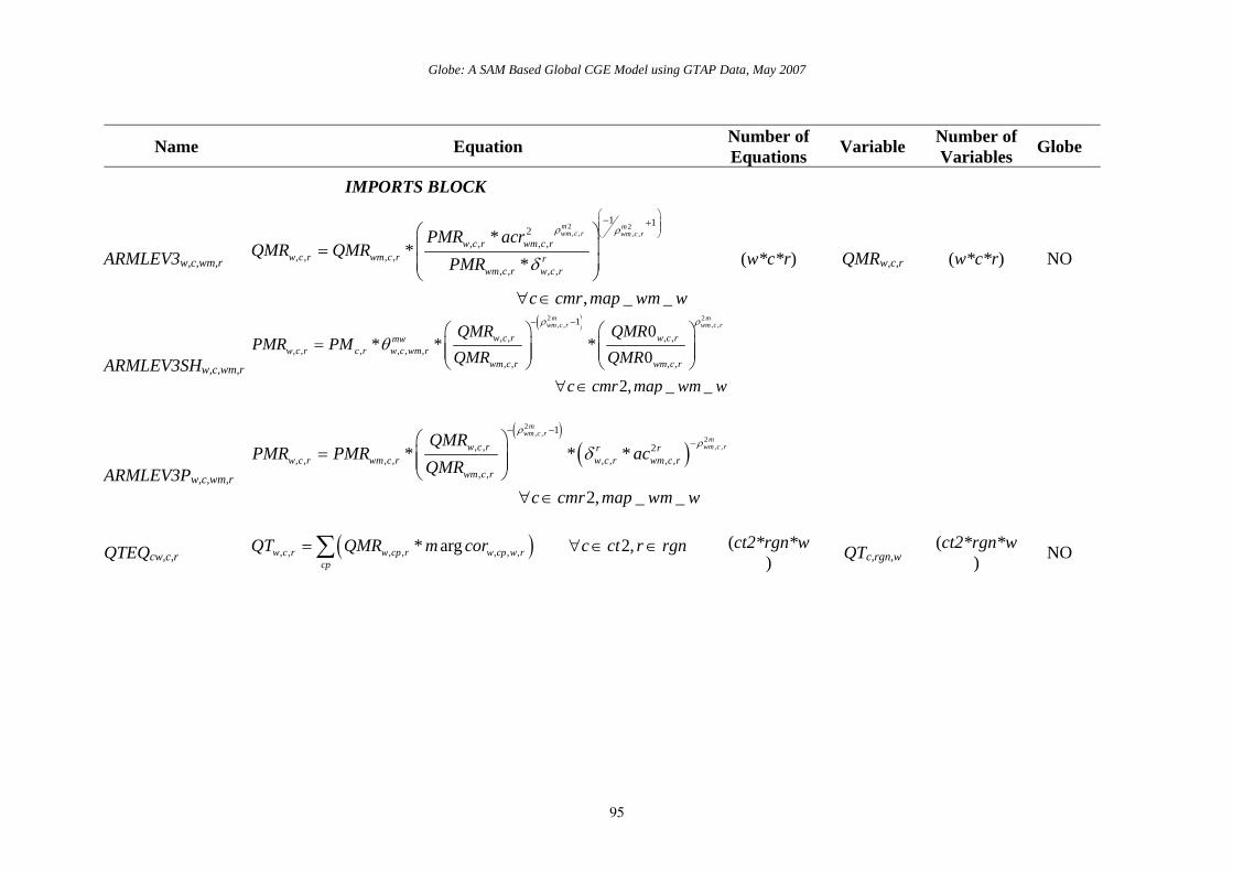
The composite import commodities are defined as CES aggregates of the imports from

different ‘regional’ groups (QMRw,c,r), (M8), which are themselves aggregates from individual

regions (M9). The first order conditions come from the price definition terms for composite

imports, PMc,r, (M2) and are only implemented for those cases where there were import

transactions in the base period – this is controlled by the set cmr. The formulation of (M8)

and (M9) are derived from the first-order conditions, as demonstrated in Appendix A2. This

form, with quantity of imports on the left-hand side, is used because it improves model

performance.

Import Block Equations 2

( )( )( )

, , ,

1

, , , , , ,* 1 *

,

c c cc r c r c r

c r c r c r c r c r c rQQ ac QM QD

c cx cm r rgn

ρ ρ ρδ δ⎛ ⎞⎜ ⎟−⎜ ⎟− − ⎝ ⎠= + −

∀ ∈ ∩ ∈

(M5)

( )( )

( ),

1

1, ,

, ,, ,

* * ,1

cc rc r c r

c r c rc r c r

PDQM QD c cx cm r rgn

PM

ρδδ

+⎛ ⎞⎛ ⎞⎛ ⎞⎜ ⎟⎜ ⎟= ∀ ∈ ∩ ∈⎜ ⎟⎜ ⎟ ⎜ ⎟⎜ ⎟−⎝ ⎠ ⎝ ⎠⎝ ⎠

(M6)

( )( )

, , , ,

OR ,c r c r c rQQ QD QM c cx cmn r rgn

c cxn cm r rgn

= + ∀ ∈ ∩ ∈

∀ ∈ ∩ ∈ (M7)

, ,

1( 1)

, , ,, , ,

, , ,

** 2

*

m mc r c r

wm c r c rwm c r c r r

c r wm c r

PMR acrQMR QM c cmr

PM

ρ ρ

δ

⎛ ⎞−⎜ ⎟⎜ ⎟+⎝ ⎠⎛ ⎞⎜ ⎟= ∀ ∈⎜ ⎟⎝ ⎠

(M8)

2 2, , , ,

1( 1)2

, , , ,, , , ,

, , , ,

**

*

, _ _

m mwm c r wm c r

w c r wm c rw c r wm c r r

wm c r w c r

PMR acrQMR QMR

PMR

c cmr map wm w

ρ ρ

δ

⎛ ⎞−⎜ ⎟⎜ ⎟+⎝ ⎠⎛ ⎞⎜ ⎟=⎜ ⎟⎝ ⎠

∀ ∈

(M9)

( ), , , , , , ,* arg 2,w c r w cp r w c cp rcp

QT QMR m cor c ct r rgn= ∀ ∈ ∈∑ (M10)


38

A specific quantity of trade and transport services is also associated with any imported

commodity. These services are assumed to be required in fixed quantities per unit of import

by a specific region from another specific region, (M10) where the margcorw,c,cp,r are the trade

and transport coefficients associated with a unit (quantity) import by region r from region w.

This is only implemented for trade and transport commodities (ct2) and for regions that

‘actually’ import goods (rgn).

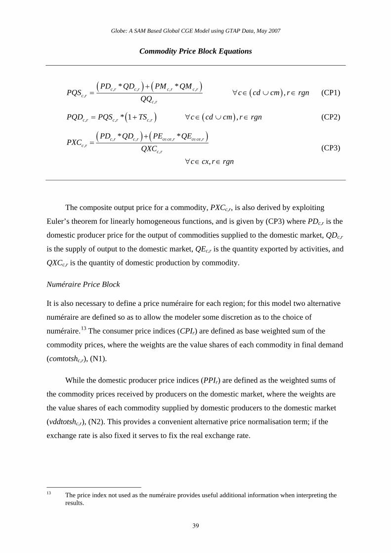
Commodity Price Block Equations

The composite price equations (CP1, CP2 and CP3) are derived from the first order

conditions for tangencies to consumption and production possibility frontiers. By exploiting

Euler’s theorem for linearly homogeneous functions the composite prices can be expressed as

expenditure identities rather than dual price equations for export transformation and import

aggregation, such that PQSc,r is the weighted average of the producer price of a commodity,

when PDc,r is the producer price of domestically produced commodities and PMc,r the

domestic price of the composite imported commodity, (CP1) where QDc,r the quantity of the

domestic commodity demanded by domestic consumers, QMc,r the quantity of composite

imports and QQc,r the quantity of the composite commodity. Notice how the commodity

quantities are the weights. This composite commodity price (CP1) does not include sales

taxes, which create price wedges between the purchaser price of a commodity (PQDc,r) and

the producer prices (PQSc,r). Hence the purchaser price is defined as the producer price plus

the sales taxes (CP2).

This formulation means that the sales taxes are levied on all sales on the domestic market,

irrespective of the origin of the commodity concerned.


39

Commodity Price Block Equations

( ) ( ) ( ), , , ,,

,

* *,c r c r c r c r

c rc r

PD QD PM QMPQS c cd cm r rgn

QQ+

= ∀ ∈ ∪ ∈ (CP1)

( ) ( ), , ,* 1 ,c r c r c rPQD PQS TS c cd cm r rgn= + ∀ ∈ ∪ ∈ (CP2)

( ) ( ), , , ,,

,

* *

,

c r c r c ce r c ce rc r

c r

PD QD PE QEPXC

QXCc cx r rgn

∈ ∈+=

∀ ∈ ∈

(CP3)

The composite output price for a commodity, PXCc,r, is also derived by exploiting

Euler’s theorem for linearly homogeneous functions, and is given by (CP3) where PDc,r is the

domestic producer price for the output of commodities supplied to the domestic market, QDc,r

is the supply of output to the domestic market, QEc,r is the quantity exported by activities, and

QXCc,r is the quantity of domestic production by commodity.

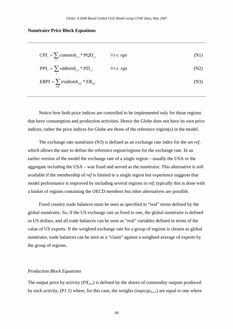
Numéraire Price Block

It is also necessary to define a price numéraire for each region; for this model two alternative

numéraire are defined so as to allow the modeler some discretion as to the choice of

numéraire.13 The consumer price indices (CPIr) are defined as base weighted sum of the

commodity prices, where the weights are the value shares of each commodity in final demand

(comtotshc,r), (N1).

While the domestic producer price indices (PPIr) are defined as the weighted sums of

the commodity prices received by producers on the domestic market, where the weights are

the value shares of each commodity supplied by domestic producers to the domestic market

(vddtotshc,r), (N2). This provides a convenient alternative price normalisation term; if the

exchange rate is also fixed it serves to fix the real exchange rate.

13 The price index not used as the numéraire provides useful additional information when interpreting the

results.


40

Numéraire Price Block Equations

, ,*r c r c rc

CPI comtotsh PQD r rgn= ∀ ∈∑ (N1)

, ,*r c r c rc

PPI vddtotsh PD r rgn= ∀ ∈∑ (N2)

*ref refref

ERPI tradtotsh ER= ∑ (N3)

Notice how both price indices are controlled to be implemented only for those regions

that have consumption and production activities. Hence the Globe does not have its own price

indices; rather the price indices for Globe are those of the reference region(s) in the model.

The exchange rate numéraire (N3) is defined as an exchange rate index for the set ref,

which allows the user to define the reference region/regions for the exchange rate. In an

earlier version of the model the exchange rate of a single region – usually the USA or the

aggregate including the USA – was fixed and served as the numéraire. This alternative is still

available if the membership of ref is limited to a single region but experience suggests that

model performance is improved by including several regions in ref; typically this is done with

a basket of regions containing the OECD members but other alternatives are possible.

Fixed country trade balances must be seen as specified in “real” terms defined by the

global numéraire. So, if the US exchange rate as fixed to one, the global numéraire is defined

as US dollars, and all trade balances can be seen as “real” variables defined in terms of the

value of US exports. If the weighted exchange rate for a group of regions is chosen as global

numéraire, trade balances can be seen as a “claim” against a weighted average of exports by

the group of regions.

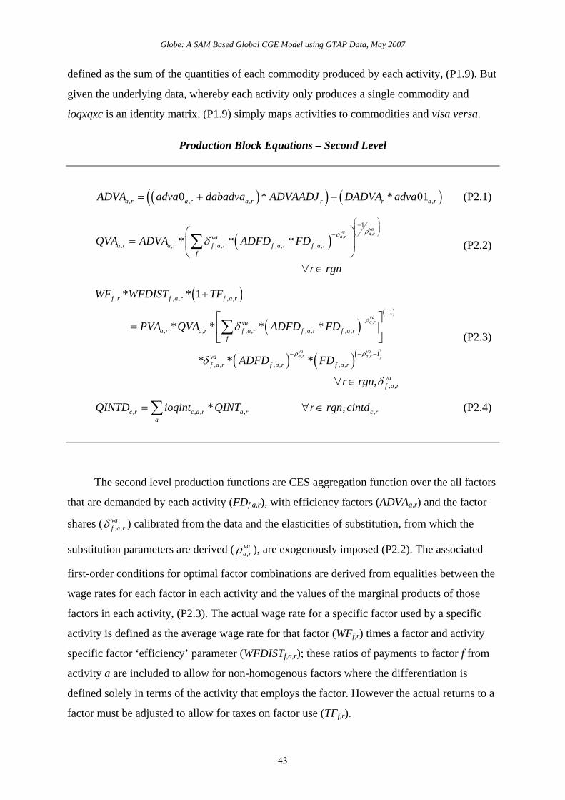
Production Block Equations

The output price by activity (PX,a,r) is defined by the shares of commodity outputs produced

by each activity, (P1.1) where, for this case, the weights (ioqxcqxa,c,r) are equal to one where


41

the commodities and activities match and zero otherwise, i.e., there is a one to one mapping

between the commodity and activity accounts. The weights are derived from the information

in the supply or make matrix.14

The value of output by activity is defined as the activity price (PXa,r) less production

taxes (TXa,r) times the volume of output (QXa,r). This revenue must be divided between

payments to primary inputs – the price of value added (PVAa,r) times the quantity of value

added (QVAa,r) – and intermediate inputs – the price of aggregate intermediate inputs

(PINTa,r) times the volume of aggregate intermediate inputs (QINTa,r) (P1.2). Given the

assumption that intermediate inputs are used in fixed (volume) proportions, the price of

aggregate intermediate inputs (PINTa,r) is defined as the weighted average price of the

intermediate inputs where the weights are the (normalised) input-output coefficients (P1.3).

The default top level production function (P1.5), is a CES aggregation of aggregate

primary and intermediate inputs, where the first order conditions for profit maximization

(P1.6) determine the optimal ratio of the inputs. The efficiency factor (ADXa,r) and the factor

shares parameters ( ,x

a rδ ) are calibrated from the data and the elasticities of substitution, from

which the substitution parameters are derived ( ,xa rρ ), are exogenously imposed. Note in this

case the efficiency factor is declared as variable and is determined by (P1.4), where adx0a,r is

the vector of efficiency factors in the base solution, dabadxa,r is a vector of absolute changes

in the vector of efficiency factors, ADXADJr is a variable whose initial value is ONE, DADXr

is a variable whose initial value is ZERO and adx01c is a vector of zeros and non zeros.15 In

the base solution the values of adx0a,r and dabadxa,r are all ZERO and ADXADJr and DADXr

are fixed as their initial values – a closure rule decision –then the applied efficiency factors

are those from the base solution. This formulation allows flexibility in the formulation of the

efficiency parameter that is especially useful in the context of a dynamic model – the structure

of the equation is identical to that used for the tax rate equations and a description of its

operation is provided when describing the tax rate equations.

14 When using GTAP data, ioqxcqxa,c,r is always a diagonal matrix. 15 Typically the values are either one or zero, i.e., the adjustment factor is switched on or off. Non zero

values other than one switch on the adjustment factor and allow a more complex set of adjustments although it is important to be careful about the rationale for such a set of adjustments.


42

Production Block Equations – Top Level

, , , ,*a r a c r c rc

PX ioqxcqx PXC r rgn= ∀ ∈∑ (P1.1)

( ) ( ) ( ), , , , , , ,* 1 * * *a r a r a r a r a r a r a rPX TX QX PVA QVA PINT QINT

r rgn

− = +

∀ ∈ (P1.2)

, , , ,*a r c a r c rc

PINT ioqint PQD r rgn= ∀ ∈∑ (P1.3)

( )( ) ( ), , , ,0 * * 01a r a r a r r r a rADX adx dabadx ADXADJ DADX adx= + + (P1.4)

( ) ( ) ( ), , ,

1

, , , , , ,* * 1 *

,

x x xa r a r a rx x

a r a r a r a r a r a rQX ADX QVA QINT

r rgn a aqx

ρ ρ ρδ δ

−− −⎡ ⎤= + −⎢ ⎥⎣ ⎦

∀ ∈ ∈

(P1.5)

( )( ),

11

, ,, ,

, ,

* * ,1

xa rx

a r a ra r a r x

a r a r

PINTQVA QINT r rgn a aqx

PVA

ρδδ

⎛ ⎞⎜ ⎟⎜ ⎟+⎝ ⎠⎛ ⎞⎛ ⎞⎛ ⎞

⎜ ⎟⎜ ⎟= ∀ ∈ ∈⎜ ⎟ ⎜ ⎟⎜ ⎟−⎝ ⎠ ⎝ ⎠⎝ ⎠ (P1.6)

, , ,* ,a r a r a ra

QINT ioqintqx QX r rgn a aqxn= ∀ ∈ ∈∑ (P1.7)

, , ,* ,a r a r a ra

QVA ioqvaqx QX r rgn a aqxn= ∀ ∈ ∈∑ (P1.8)

, , , ,*c r a c r a ra

QXC ioqxcqx QX r rgn= ∀ ∈∑ (P1.9)

The production function (P1.5) is only implemented for members of the set aqx; for its

complement, aqxn, the CES function is replaced by Leontief functions. These require that

aggregate intermediate inputs (P1.7) and aggregate values added (P1.8) are fixed proportions

of the volumes of output. If there are no intermediate inputs used by an activity the top level

functions is automatically Leontief, and the user is able to determined the minimum costs

share of intermediate inputs below which the Leontief assumption is imposed automatically

after the user defines the share – the default is 10 percent.

Finally it is necessary to define the relationship between activity and commodity

outputs, which is the counterpart to the price equation linking commodity and activity prices

(P1.1). This is defined as a simple linear relationship whereby the commodity output is


43

defined as the sum of the quantities of each commodity produced by each activity, (P1.9). But

given the underlying data, whereby each activity only produces a single commodity and

ioqxqxc is an identity matrix, (P1.9) simply maps activities to commodities and visa versa.

Production Block Equations – Second Level

( )( ) ( ), , , ,0 * * 01a r a r a r r r a rADVA adva dabadva ADVAADJ DADVA adva= + + (P2.1)

( ) ,,

1

, , , , , , , ,* * *vava a ra rva

a r a r f a r f a r f a rf

QVA ADVA ADFD FD

r rgn

ρρδ

⎛ ⎞−⎜ ⎟⎜ ⎟⎝ ⎠−⎛ ⎞

= ⎜ ⎟⎝ ⎠

∀ ∈

∑ (P2.2)

( )

( )( )

( ) ( )( )

,

, ,

, , , , ,

1

, , , , , , , ,

1

, , , , , ,

, ,

* * 1

* * * *

* * *

,

vaa r

va vaa r a r

f r f a r f a r

vaa r a r f a r f a r f a r

f

vaf a r f a r f a r

vaf a r

WF WFDIST TF

PVA QVA ADFD FD

ADFD FD

r rgn

ρ

ρ ρ

δ

δ

δ

−−

− − −

+

⎡ ⎤= ⎢ ⎥

⎣ ⎦

∀ ∈

∑ (P2.3)

, , , , ,* ,c r c a r a r c ra

QINTD ioqint QINT r rgn cintd= ∀ ∈∑ (P2.4)

The second level production functions are CES aggregation function over the all factors

that are demanded by each activity (FDf,a,r), with efficiency factors (ADVAa,r) and the factor

shares ( , ,vaf a rδ ) calibrated from the data and the elasticities of substitution, from which the

substitution parameters are derived ( ,vaa rρ ), are exogenously imposed (P2.2). The associated

first-order conditions for optimal factor combinations are derived from equalities between the

wage rates for each factor in each activity and the values of the marginal products of those

factors in each activity, (P2.3). The actual wage rate for a specific factor used by a specific

activity is defined as the average wage rate for that factor (WFf,r) times a factor and activity

specific factor ‘efficiency’ parameter (WFDISTf,a,r); these ratios of payments to factor f from

activity a are included to allow for non-homogenous factors where the differentiation is

defined solely in terms of the activity that employs the factor. However the actual returns to a

factor must be adjusted to allow for taxes on factor use (TFf,r).


44

The efficiency factors are declared as variables (P2.1), where adva0a,r is the vector of

efficiency factors in the base solution, dabadvaa,r is a vector of absolute changes in the vector

of efficiency factors, ADVAADJr is a variable whose initial value is ONE, DADVAr is a

variable whose initial value is ZERO and adva01a,r is a vector of zeros and non zeros.16 In the

base solution the values of adva0a,r and dabadvaa,r are all ZERO and ADVAADJr and

DADVAr are fixed as their initial values – a closure rule decision – then the applied efficiency

factors are those from the base solution.

Since production uses intermediate inputs, it is also necessary to specify the demand for

intermediate inputs (QINTDc,r). This is done from the perspective of commodity demands,

i.e., it is summed over activities to produce the demand for intermediate inputs by commodity

rather than by activity (P2.4).

Factor Block Equations

The total income received by each factor account (YFf) is defined as the summation of the

earnings of that factor across all activities (F1). However, only a proportion of total factor

income is available for distribution to the domestic institutional accounts (YFDISTf,r). First

allowance must be made for depreciation, which it is assumed takes place at fixed rates

(deprecf,r) relative to factor incomes and the payment of factor income taxes (TYFf,r) (F2).

16 Typically the values are either one or zero, i.e., the adjustment factor is switched on or off. Non zero

values other than one switch on the adjustment factor and allow a more complex set of adjustments although it is important to be careful about the rationale for such a set of adjustments.


45

Factor Block Equations

, , , , , ,* *f r f r f a r f a ra

YF WF WFDIST FD r rgn= ∀ ∈∑ (F1)

( )( ) ( ), , , , ,* * 1f r f r f r f r f rYFDIST YF deprec YF TYF

r rgn

= − −

∀ ∈ (F2)

Household Block Equations

Households acquire income from only one source in this model; the sale of factor services.

Therefore household income (YHh,r) is defined simply as the sum of factor incomes available

for distribution. In this variant allowance is made for the possibility of multiple households by

including a set of distribution parameters (hvashh,f,r) that are defined as the shares of each

factor demanded in the economy that is supplied by each household. In the case of one

household all the shares equal one.

Household Block Equations

, , , ,*h r h f r f rf

YH hvash YFDIST r rgn= ∀ ∈∑ (H1)

( )( ) ( ), , , ,* 1 * 1h r h r h r h rHEXP YH TYH SHH r rgn= − − ∀ ∈ (H2)

( ), , , , , ,

, , , , , ,

* *

* *

c h r c r c r c h r

c h r h r c r c h rc

QCD PQD PQD qcdconst

HEXP PQD qcdconst r rgnβ

=

⎛ ⎞+ − ∀ ∈⎜ ⎟⎝ ⎠

∑ (H3)

Household consumption demand is derived in two stages. In the first stage (H2)

household consumption expenditures (HEXPh,r) are defined as household incomes after the

payment of direct taxes and savings and inter household transfers. Note how the saving rates


46

are defined as proportions of after tax incomes that are saved; this is important for the

calibration of the income tax and savings parameters.

The household utility functions are assumed to be Stone-Geary, i.e., a linear expenditure

system, which means that household consumption demand consists of two components,

‘subsistence’ demand (qcdconstc,h,r) and ‘discretionary’ demand, and the equation must

therefore capture both elements. Discretionary demand is defined as the marginal budget

shares (β) spent on each commodity out of ‘uncommitted’ income, i.e., household

consumption expenditure less total expenditure on ‘subsistence’ demand. The quantities of

each commodity demanded by the household are then defined by the shares of household

consumption expenditure. The Stone-Geary function collapses to a Cobb-Douglas utility

function if all the income elasticities of demand are set equal to one and the Frisch parameter,

the elasticity of the marginal utility of income, is also set to one. One advantage of the Cobb-

Douglas specification is that it results in the changes in the values for household consumption

expenditures (HEXPh,r) being equal to the changes in an equivalent variation measure of

household welfare.

Government Tax Block Equations

There are seven tax instruments. Each is defined as a simple ad valorem rate dependent upon

the values of imports, exports, sales, production and factor use by activities and the levels of

factor and household and income. The ‘tax’ rates are all declared as variables.

All tax rates are variables in this model and for each tax instrument a series of factors

are declared to facilitate policy experiments. The tax rates in the base solution are defined as

parameters, e.g., tm0w,c,r are the import tariff rates by commodity c imported from region w in

region r in the base solution, and the tax rate equations then allow for varying the tax rates in

four different ways. Two of the methods use variables that can be solved for optimum values

in the model according to the choice of closure rule and two methods allow for deterministic

adjustments to the structure of the tax rates. The operations of these methods are discussed in

detail only for the equations for import duties while the other equations are simply reported.


47

Government Tax Rates Equations

( )( ) ( ), , , , , , , ,0 * * 01w c r w c r w c r r r w c rTM tm dabtm TMADJ DTM tm c cmr= + + ∀ ∈ (T1.1)

( )( ) ( ), , , , , , , ,0 * * 01c w r c w r c w r r r c w rTE te dabte TEADJ DTE te c cer= + + ∀ ∈ (T1.2)

( )( ) ( )( )

, , , ,0 * * 01

,c r c r c r r r c rTS ts dabts TSADJ DTS ts

r rgn c cd cm

= + +

∀ ∈ ∈ ∪ (T1.3)

( )( ) ( ), , , ,0 * * 01a r a r a r r r a rTX tx dabtx TXADJ DTX tx r rgn= + + ∀ ∈ (T1.4)

( )( ) ( ), , , ,0 * * 01f r f r f r r r f rTYF tyf dabtyf TYFADJ DTYF tyf r rgn= + + ∀ ∈

(T1.5)

( )( ) ( ), , , ,0 * * 01h r h r h r r r h rTYH tyh dabtyh TYHADJ DTYH tyh r rgn= + + ∀ ∈

(T1.6)

( )( ) ( ), , , , , , , ,0 * * 01f a r f a r f a r r r f a rTF tf dabtf TFADJ DTF ty r rgn= + + ∀ ∈

(T1.7)

In the import tariff rate equation (T1.1) tm0w,c,r is the vector of import duties in the base

solution, dabtmw,c,r, is a vector of absolute changes in the vector of import duties taxes,

TMADJr is a region specific variable whose initial value is ONE, DTMr is a region specific

variable whose initial value is ZERO and tm01w,c,r is a vector of zeros and non zeros. In the

base solution the values of tm01w,c,r and dabtm w,c,r are all ZERO and TMADJr and DTMr are

fixed as their initial values – this is a closure rule decision. Given this decision the model

treats the tax rates as (fixed) parameters and the applied import tariffs are those from the base

solution. The different methods of adjustment can be considered in turn.

1. If TMADJr for one region is made a variable, which requires the fixing of

another variable for that region, and all other initial conditions hold then the

solution value for TMADJr yields the optimum equiproportionate change in the

import duty rates necessary to satisfy model constraints, e.g., if TMADJr equals

1.1 then all applied (non zero) import duty rates (that are found in the base data)

for the specified region are increased by 10%.


48

2. If any element of dabtmw,c,r is not zero, and all the other initial conditions hold,

then an absolute change in the initial import tariff rate for the relevant

commodity is imposed, e.g., if tm0w,c,r for one element of c is 0.1 (a 10% import

duty) and dabtmw,c,r for that element is 0.05, then the applied import tariff rate is

0.15 (15%).

3. If TMADJr for one region is made a variable, which requires the fixing of

another variable for that region, any elements of dabtmw,c,r are non zero and all

other initial conditions hold, then the solution value for TMADJr yields the

optimum equiproportionate change in the applied import duty rates, i.e., tm0w,c,r

+ dabtmw,c,r (and these applied rates can be different from those in the base in

which dabtmw,c,r is set at zero).

4. If DTMr for one region is made a variable, which requires the fixing of another

variable for that region, AND at least one element of tm01w,c,r is ONE then the

subset of elements of tm0w,c,r identified by tm01w,c,r are allowed to (additively)

increase by an equiproportionate amount determined by the solution value for

DTMr and the initial values of the import duty rates, e.g., if food products are to

be excluded from the change in tax rates then the elements of tm01w,c,r

corresponding to the food commodities are (left as) zeros. Note how in this case

it is necessary to both ‘free’ a variable and give values to a parameter for a

solution to emerge. If the change in the applied tax rates is to be other than

equiproportionate then values of tm01w,c,r other than one can be applied, e.g., if

the changes in the import duties on food products are to be half those on other

sectors then the elements of tm01w,c,r corresponding to the food commodities can

be set to 0.5 and for the other commodities can be set to 1.

This combination of alternative adjustment methods covers the range of common tax

rate adjustments used in the majority of applied applications while being flexible and easy to

use. However experience has shown that when working with GTAP data it is very important

to check the tax rates that are applied in the base solution; in some aggregations some of the

applied tax rates only differ marginally from zero but are a mix of negatives and positives, in

such cases it may be necessary to exogenously reset the tax rates to avoid apparently odd


49

results. All the model parameters are exported to a GDX file and can be easily accessed using

GDXViewer and/or SeeResults.17

The other tax rate equations follow the same structure. Export taxes (TEc,r) are defined

in (T1.2), sales taxes (TSc,r) are defined in (T1.3), production tax rates (TXa,r) are defined in

(T1.4), factor income tax rates (TYFf,r) are defined in (T1.5), household income rates (TYHh,r)

are defined in (T1.6) and factor use tax rates (TFf,r) are defined in (T1.7.)

Government Tax Revenues Equations

( ), , , , , ,* * *r w c r w c r r w c rw c

MTAX TM PWM ER QMR

r rgn

=

∀ ∈

∑∑ (T2.1)

( ), , , , , ,* * *r c w r c w r r c w rw c

ETAX TE PWE ER QER

r rgn

=

∀ ∈

∑∑ (T2.2)

, , , , , , ,* *r c r c r c r c h r c r c rc h

STAX TS PQS QINTD QCD QGD QINVD

r rgn

⎛ ⎞⎛ ⎞= + + +⎜ ⎟⎜ ⎟

⎝ ⎠⎝ ⎠∀ ∈

∑ ∑ (T2.3)

( ), , ,* *r a r a r a ra

ITAX TX PX QX r rgn= ∀ ∈∑ (T2.4)

( )( )( ), , , ,* *r f r f r f r f rf

FYTAX TYF YF deprec YF

r rgn

= −

∀ ∈

∑ (T2.5)

( ), ,*r h r h rh

HTAX TYH YH r rgn= ∀ ∈∑ (T2.6)

( ), , , , , , ,* * *r f a r f r f a r f a rf a

FTAX TF WF WFDIST FD r rgn= ∀ ∈∑∑ (T2.7)

The government tax revenue equations simply sum the revenues from each different tax

instrument for each region. These are not strictly necessary for the model since the equations

could be collapsed into a single government income equation (see G1 below). However it is

useful to carry around these additional variables since they can then be used in model closures

to accommodate specific government tax revenue objectives and they are useful sources of

17 See Section 6 on complementary programmes.


50

information when analysing simulation results.18 Import duty revenues (MTAXr) are defined

as total import duty revenue in region r (T2.1); Export tax revenues (ETAXr) are defined as

total export tax revenue in region r (T2.2); sales tax revenues (STAXr) are defined as total

sales tax revenue in region r (T2.3); production tax revenues (ITAXr) are defined as total

production tax revenue in region r (T2.4); factor income tax revenues (FYTAXr) are defined as

total factor income tax revenue in region r (T2.5); household income tax revenues (HTAXr)

are defined as total household income tax revenue in region r (T2.6) and factor use tax

revenues (FTAXr) are defined as total factor use tax revenue in region r (T2.7).

Government Block Equations

Government income (YGr) is defined as the sum of government tax revenues (G1), where the

tax revenues are treated as expenditures by the accounts paying the taxes and hence are

defined in the tax block. While this approach adds equations it has the arguable advantage of

being more transparent and easier to modify.

Other Government Equations

r r r r r r r rYG MTAX ETAX STAX ITAX FYTAX HTAX FTAXr rgn

= + + + + + +∀ ∈

(G1)

, , *c r c r rQGD qgdconst QGDADJ r rgn= ∀ ∈ (G2)

, ,*r c r c rc

EG PQD QGD r rgn= ∀ ∈∑ (G3)

Government demand for commodities (G2) is assumed fixed in real terms, i.e., the

volume is fixed, but can be scaled or allowed to vary using an adjustment factor (QGDADJr).

The precise specification depends upon the choice of closure rule (see below). Thereafter

Government consumption expenditure (EGr) is defined as the sum of commodity

consumption (G3). The advantage of separately expressing the volume and value of

government expenditures is the increased flexibility it provides in the choice of closure rules

18 It is a simple matter to generate such aggregates from model results as part of the reported output of the

simulations. The trade off between the increase in model ‘size’ associated with extra variables and reduction in the size of the files that generate results is a matter of judgement; the general approach used


51

for the government account. This arrangement allows adjustment of government demand

either through the volume, or the expenditure or the value share of final demand (see below).

Kapital Account Block Equations

Income to the capital (savings and investment) account, total savings, comes from household

savings, depreciation allowances, government savings (KAPGOVr) and the surplus on the

capital account of the balance of payments (KAPWORr), and hence is simply defined as the

sum of savings by domestic and ‘foreign’ agents (K1.2).

In this model the household savings rates are declared as variables (SHHh,r) that define

the proportions of income saved after the payment of income taxes. The savings rate

equations (K1.1) used the same adjustment structure as used for the tax rate equations; hence

shh0h,r are the base solution savings rates dabshhh,r are absolute changes in the base savings

rates, SADJr are multiplicative adjustment factors, DSHHr are additive adjustment factors and

shh01h,r is a matrix of zero and non zero values that determine for which households and

regions the savings rates can adjust additively. Note that household savings are taken out of

after-tax income.

Savings Block Equations

( )( ) ( ), , , ,0 * * 01h r h r h r r r h rSHH shh dabshh SADJ DSHH shh r rgn= + + ∀ ∈ (K1.1)

( )( ) ( )

( )

, , ,

, ,

* 1 *

*

*

r h r h r h rh

f r f rf

r r r

TOTSAV YH TYH SHH

deprec YF

KAPGOV KAPWOR ER r rgn

⎛ ⎞= −⎜ ⎟⎝ ⎠

+

+ + ∀ ∈

∑

∑ (K1.2)

Government savings are calculated as residual (see the KAPGOVr equations, MC3.1,

below). The surplus on the capital account (KAPWORr) is defined in terms of the foreign

currency (see MC3.4 and MC3.3) and therefore the exchange rate appears in this equation

(this is a matter of preference).

here is to include as variable such aggregates that may have substantive benefits in terms of transparency


52

Investment demand is modeled in a similar way to government demand. Demand for

commodities (K2.1) used in investment is assumed to be in fixed volumes (qinvdconstc,r)

multiplied by an investment-scaling variable (IADJr) that can accommodate changes in the

exogenously determined level of investment and/or changes in the availability of funds for

investment. The second stage (K2.2) captures the price effect by identifying the total value of

investment (INVESTr). This arrangement allows adjustment of investment demand either

through the volume, or the expenditure or the value share of final demand (see below).

Investment Block Equations

, ,*c r r c rQINVD IADJ qinvdconst r rgn= ∀ ∈ (K2.1)

( ), ,*r c r c rc

INVEST PQD QINVD r rgn= ∀ ∈∑ (K2.2)

Market Clearing Block Equations

In the base solution to the model the market clearing, or equilibrium, conditions are relatively

straightforward. Factor supplies must equal factor demands (MC1) and (composite)

commodity supplies must equal (composite) commodity demands (MC2). It appears that there

is no equilibrium condition for the supply of domestic output to the domestic market. In fact

this is achieved through the commodity output equation (P1.9), which could have been treated

as a market clearing equation.

and simulation formulation.


53

Factor Account Equations

, , ,f r f a ra

FS FD r rgn= ∀ ∈∑ (MC1.1)

Commodity Account Equations

( )

, , , , , ,

,

c r c r c h r c r c rh

QQ QINTD QCD QGD QINVD

c cd cm r rgn

= + + +

∀ ∈ ∪ ∈

∑ (MC2.1)

The government account is cleared by defining government savings (KAPGOVr) as the

difference between government income and government expenditure on consumption and

transfers; hence government savings are explicitly treated as a residual, (MC3.1). The

deficit/surplus on the current account is computed in two-stages. First the bilateral trade

balances (KAPREGw,r) are calculated as the difference in the values of imports and exports,

for first the trade flows between regions other than Globe (MC3.2) and then for trade between

Globe and all other regions (MC3.3) – the latter being the trade balances on margins trade.

These transactions are valued in terms of the global numéraire. Then the overall balance of

trade (KAPWORr) is computed for each region, (MC3.4). Finally the commodity trade

balance for Globe is defined (MC3.5), since this should be zero by definition a slack variable

(GLOBESLACK) is attached.


54

Investment and Savings Account Equations

r r rKAPGOV YG EG r rgn= − ∀ ∈ (MC3.1)

, , , , , , , , ,* *w r w c r w c r c w r c w rc c

KAPREG PWMFOB QMR PWE QER

w wgn

⎛ ⎞ ⎛ ⎞= −⎜ ⎟ ⎜ ⎟

⎝ ⎠ ⎝ ⎠∀ ∈

∑ ∑ (MC3.2)

, , , , , , , ,* *w r c r w c r c w r c w rc w c

KAPREG PT QT PWE QER

w wgn

⎛ ⎞ ⎛ ⎞= −⎜ ⎟ ⎜ ⎟

⎝ ⎠ ⎝ ⎠∀ ∉

∑∑ ∑ (MC3.3)

,r w rw

KAPWOR KAPREG r= ∀∑ (MC3.4)

( ) ( ), , , , , , , ,* *

2,

w c r w c r c w r c w rw w

PWM QMR PWE QER GLOBESLACK

c ct r rgn

= +

∀ ∈ ∉

∑ ∑ (MC3.5)

The commodity trade accounts define the market clearing conditions for bilateral trade.

The fob prices for imports (PWMFOBw,c,r) for all imports by destination and source must be

equal to the fob prices for exports (PWEc,w,r) by source and destination (MC4.1). In addition

the quantities of imports (QMRw,c,r) for all imports by destination and source must be equal to

the quantities of exports (QERc,w,r) by source and destination (MC4.2). These equations are

not completely straightforward since it is necessary in their implementation to employ

mappings between exporting and importing regions that require the ‘switching’ of labels on

accounts within the equation.

Commodity Trade Account Equations

, , , , , _ _ , _ _w c r c w rPWMFOB PWE c cmr map r w map w r= ∀ ∈ (MC4.1)

, , , , , _ _ , _ _w c r c w rQMR QER c cmr map r w map w r= ∀ ∈ (MC4.2)

The trade consistency equations do not however deal with the requirements for market

clearing with respect to the trade transactions undertaken by the Globe region. However


55

similar conditions apply for the margins trade. These require that the total demand for each

and every trade and transport service (QTw,c,r) is exactly equal to the exports of that service by

Globe (QERc,w,”glo”) and the import prices of margin services (PTc,r) must equal the export

prices (fob) from Globe; these conditions are imposed by (MC5.1) and (MC5.2) respectively.

Margin Trade Account Equations

, , , ," " 2,w c r c w glow w

QT QER c ct r rgn= ∀ ∈ ∈∑ ∑ (MC5.1)

, , ," " 2,c r c w gloPT PWE c ct r rgn= ∀ ∈ ∈ (MC5.2)

The absorption closure equations exist to support closure rules choices relating to the

distribution of final demand between the institutions within regions. The value of final

demand by region (VFDOMDr) is simply the sum of the value of final demand across the

three sources of final demand – households, government and investment (MC6.1). The value

share of final demand accounted for by investment (INVESTSHr) is defined in (MC6.2), and

the value share of final demand accounted for by government (VGDSHr) is defined in

(MC6.3). No similar expression exists for the households because household expenditure are

defined after taxes and savings and it is difficult to justify setting the household shares

relative to the value of total final demand since this would nullify the distributional

consequences of a policy shock. If the expenditure shares by investment and government are

fixed then the expenditure share of ALL households will by definition be fixed and HEXPr

could be fixed for individual households if there was good reason.


56

Absorption Closure Equations

, , , , ,*r c r c h r c r c rc h

VFDOMD PQD QCD QGD QINVD

r rgn

⎛ ⎞⎛ ⎞= + +⎜ ⎟⎜ ⎟⎝ ⎠⎝ ⎠

∀ ∈

∑ ∑ (MC6.1)

*r r rINVESTSH VFDOMD INVEST r rgn= ∀ ∈ (MC6.2)

( ), ,* *r r c r c rc

VGDSH VFDOMD PQD QGD r rgn= ∀ ∈∑ (MC6.3)

The final equations are for slacks. The satisfaction of Walras’s law requires that if all

other accounts balance then so must the final account; thus the difference between savings

and investment for all regions that save should always be zero and hence the variable

WALRASr should equal zero in (MC7.1). That this variable equals zero is a good check on the

correct specification of the model. Finally the global trade balance must by definition be zero

and hence so must KAPWORSYS (MC7.2)

Slack Equations

r r rTOTSAV INVEST WALRAS r rgn= + ∀ ∈ (MC7.1)

rrKAPWORSYS KAPWOR r rgn= ∀ ∈∑ (MC6.2)

Model Closure Conditions or Rules19

In mathematical programming terms the model closure conditions are, at their simplest, a

matter of ensuring that the numbers of equations and variables are consistent. However the

economic theoretic dimensions of model closure rules are more complex, and, as would be

expected in the context of an economic model, more important. The essence of model closure

rules is that they define important and fundamental differences in perceptions of how an


57

economic system operates (see Sen, 1963; Pyatt, 1987; Kilkenny and Robinson, 1990). The

closure rules can be perceived as operating on two levels; on a general level whereby the

closure rules relate to macroeconomic considerations, e.g., is investment expenditure

determined by the volume of savings or exogenously, and on a specific level where the

closure rules are used to capture particular features of an economic system, e.g., the degree of

intersectoral capital mobility.

This model allows for a range of both general and specific closure rules. The discussion

below provides details of some of the options available with this formulation of the model by

reference to the accounts to which the rules refer. However, as will become readily apparent

there are many permutations available, and hence this discussion deals with the general

principles rather than trying to define all possible permutations. The philosophy adopted in

the implementation of this model is to define a (minimal) base closure for the replication of

the base case and then impose closure changes within a loop in the experiment/simulation file.

This approach allows substantial flexibility in the definition of policy simulations while

simultaneously allowing sensitivity testing of the chosen model closures. For the base

solution the choice of model closure is basically a neoclassical closure; the reason for

choosing this closure is NOT a statement about its appropriateness, rather it is a closure that

allows flexibility in model solution and hence simplifies the process of verifying that the

model is correctly specified and calibrated.

Foreign Exchange Account Closure

For the world numéraire the exchange rate index for the reference regions (EPRI) is fixed

(C1a), although a parameter, numerchk, is attached to allow for ease of checking the

homogeneity of the model.20 At the same time the exchange rate for Globe is fixed as equal to

the world numéraire (C1b).

The default closure for the non-Globe regions involves an assumption that the nominal

exchange rate is flexible. Hence the trade balances (KAPWORrgn) for all non Globe regions

are fixed (C1c) and the exchange rate is flexible. The most straightforward alternative is to fix

19 The term model ‘closure’ is used generically here to cover all permutations including variations in market

clearing conditions and macroeconomic closure conditions. 20 In the base and model simulations, numerchk equals one. It is a parameter attached to the world

numéraire and the regional numéraire (see C5a and C5b). To check for homogeneity, a value other than one should have no effect on real variables in the model.


58

the exchange rates for all non Globe regions (C1d) and unfix the trade balances. However

there are clearly a range of permutations whereby the exchange rates for some regions are

flexible while for others they are fixed.21

Foreign Exchange Account Closure

0 *EPRI EPRI numerchk= (C1a)

" " 0 *gloER EPRI numerchk= (C1b)

rgn rgnKAPWOR KAPWOR= . (C1c)

rgnrgnER ER= (C1d)

Capital Account Closure

This discussion of the closure rules for the capital account begins by abstracting from some of

the complexities into interactions between different closure conditions. To ensure that

aggregate savings equal aggregate investment, the determinants of either savings or

investment must be fixed. The default closure for this account requires the assumption that

savings rates are exogenously determined which involves fixing both the multiplicative

savings rates adjusters (SADJr) (C2a) and the additive savings rates adjusters (DSHHr) (C2b)

and allowing the savings rates to be fixed – typically at their base rates. With such a savings-

driven closure the value and volume of investment must be free to vary.

Choosing an investment-driven closure requires making two distinct choices; first, is

the level investment to be determined in terms of volume, value or expenditure share of final

demand, and second, will savings adjust in a multiplicative or additive mode. Clearly, again,

it is possible that the choices will vary by region. If the investment volume adjuster (IADJr) is

fixed (C2c), then the value of investment expenditure might change due to changes in the

prices of investment commodities (PQDc,r). If the value of investment (INVESTr) is fixed

(C2d) then both the value of savings must be free to adjust as must the actual volume of

21 The option is provided in the programme to control choice of these, and several other, closures by

selection of regions to assign to a set and its complement.


59

investment. The same applies if the shares of investment expenditures in final demand

(INVESTSHr) are fixed (C2e).

Capital Account Closure

r rSADJ SADJ= (C2a)

r rDSHH DSHH= (C2b)

rrIADJ IADJ= (C2c)

rrINVEST INVEST= (C2d)

rrINVESTSH INVESTSH= (C2e)

Fixing savings, and thus deeming the economy to be savings-driven, could be termed a

Neo-Classical approach. Closing the economy by fixing investment however makes the model

reflect a Keynesian investment-driven assumption for the operation of an economy.

However there are potentially important interaction effects. Note that there are other

sources of potential savings for region – the government and the trade balances. The

magnitudes of these other savings sources can also be controlled through the closure rules

(see below). Consequently there will clearly be an important interdependence between the

choices of closure rules for different accounts; the most obvious one to be aware of is the

interaction between household savings rates and household income tax rates when tax rates

are made flexible and the level of government savings/deficit is fixed.

Government Account Closure

The closure rules for the government account are slightly more complex because they are

important components of the model that are used to investigate fiscal policy considerations.

The base specification uses the assumption that government savings are a residual; when the

determinants of government income, i.e., tax rates, remittances etc., and expenditure are

‘fixed’, government savings must be free to adjust.


60

Thus in the base specification all the tax rates are fixed by declaring the tax rates as

parameters and then fixing all the tax rate scaling factors (C3.1a – C3.1n). Consequently any

changes in tax revenue to the government are consequences of changes in the other variables

that enter into the tax income equations (T2.1 to T2.6). Controlling the volumes of

commodity demand (QGDc,r) in the base specification government expenditure is then

achieved by fixing the volumes of commodity demand (QGDc,r) through the government

demand adjuster (QGDADJr) (T3.2a). Notice however that since prices are typically free to

change it is necessary to ensure that both government expenditure (EGr) in (C3.2b) and the

share of government expenditure in final demand (VGDSHr) in (C3.2c) must be flexible.


61

Tax Rate and Revenue Closure

rrTMADJ TMADJ= (C3.1a)

r rTEADJ TEADJ= (C3.1b)

r rTSADJ TSADJ= (C3.1c)

r rTXADJ TXADJ= (C3.1d)

r rTYFADJ TYFADJ= (C3.1e)

r rTYHADJ TYHADJ= (C3.1f)

r rTFADJ TFADJ= (C3.1g)

rrDTM DTM= (C3.1h)

rrDTE DTE= (C3.1i)

rrDTS DTS= (C3.1j)

rrDTX DTX= (C3.1k)

rrDTYF DTYF= (C3.1l)

rrDTYH DTYH= (C3.1m)

rrDTF DTF= (C3.1n)

This specification ensures that all the parameters that the government can/does control

are fixed and consequently that the only determinants of government income and expenditure

that are free to vary are those that the government does not directly control. Hence the

equilibrating condition is that government savings, the internal balance (KAPGOVr), is not

fixed in (C3.2d).

The number of possible permutations for closing the government account for each

region is consequently substantial. Practical experience indicates that great care is needed

when adjusting the government closure rules to avoid both unbalancing the model and


62

imposing closure rules that are contradictory.22 A common change is to require that the

government’s savings/deficit is fixed; this requires fixing KAPGOVr in C3.2d, in which case

either government income or expenditure must be free to adjust. Such a condition might

reasonably be expected in many circumstances, e.g., the government might define an

acceptable level of borrowing or such a condition might be imposed externally.

Government Expenditure and Savings Closure

rrQGDADJ QGDADJ= (C3.2a)

r rEG EG= (C3.2b)

r rVGDSH VGDSH= (C3.2c)

r rKAPGOV KAPGOV= (C3.2d)

In its simplest form this can be achieved by allowing one of the previously fixed tax rate

adjusters (C3.1a to C3.1n) to vary. Thus if the sales tax adjuster (TSADJr) is made variable

then the sales tax rates will be varied equiproportionately so as to satisfy the internal balance

condition. More complex experiments might result from the imposition of multiple

conditions, e.g., a halving of import duty rates coupled with a reduction in government deficit,

in which case the variables TMADJr and KAPGOVr would also require resetting. But these

conditions might create a model that is infeasible, e.g., due to insufficient flexibility through

the import duties mechanism, or unrealistically high rates of sales taxes. In such

circumstances it may be necessary to allow adjustments in multiple tax adjusters. One method

then would be to fix the tax adjusters to move in parallel with each other.

However, if the adjustments only take place through the tax rate scaling factors the

relative tax rates will be fixed. To change relative tax rates it is necessary to change the

relevant tax parameters. Such changes would be implemented in policy experiment files by

changing the values of the parameters that determine relative tax rates.

22 The most common problems with contradictory government closure rules relate to the interactions

between the government and capital (investment) accounts, in particular when a combination of flexible savings and tax rates producing mutually contradictory effects.


63

Note also that as with the investment account, there is a needed care over setting the

constraints on government demand. If the government demand volume adjuster (QGDADJr)

is fixed (C3.2a), then the value of government expenditure might change due to changes in

the prices of commodities (PQDc,r). If the value of government expenditure (EGr) is fixed

(C3.2b) then both government savings must be free to adjust as must the actual volume of

expenditure, when tax rates are exogenous. The same applies if the shares of government

expenditures in final demand (VGDSHr) are fixed (C3.2e).

Technology and Efficiency

The default assumption in the model is that efficiency, commonly called technology, is fixed.

Hence the shift parameters are assumed to be constant.

Technology Parameter Closure

,, 0a ra rADX ADX= (C4.3a)

,, 0a ra rADVA ADVA= (C4.4a)

, ,, , 0 f a rf a rADFD ADFD= (C4.5a)

Changes in efficiency can either be imposed exogenously or a technology variable can

be freed up so as to satisfy some other condition, e.g., the required efficiency gain needed to

satisfy a predetermined increase in GDP.

Numéraire

The model specification allows for a choice between two price normalisation equations, the

consumer price index (CPIr) and a producer price index (PPIr). A numéraire is needed for

each region, to serve as a base since the model is homogenous of degree zero in prices for

each region, and hence only defines relative prices.


64

Numéraire Closure

r rCPI CPI numerchk= ∗ (C5a)

r rPPI PPI numerchk= ∗ (C5b)

Factor Market Closure

The factor market closure rules are more difficult to implement than many of the other closure

rules. Hence the discussion below proceeds in three stages; the first stage sets up a basic

specification whereby all factors are deemed perfectly mobile, the second stage introduces a

more general specification whereby factors can be made activity specific and allowance can

be made for unemployed factors, while the third stage introduces the idea that factor market

restrictions may arise from activity specific characteristics, rather than the factor inspired

restrictions considered in the second stage.

Full Factor Mobility and Employment Closure

This factor market closure requires that the total supply of and total demand for factors

equate, and since the total supplies of each factor are determined exogenously this condition

is satisfied by the equilibrium condition (C6.1a). The demands for factor f by activity a in

region r and the wage rates for factors are determined endogenously. But the model

specification includes the assumption that the wage rates for factors are averages (WFf,r), by

allowing for the possibility that the payments to notionally identical factors might vary across

activities, due to activity specific ‘efficiency’ factors (WFDISTf,a,r) through the variable that

captures the ‘sectoral proportions for factor prices’. Since these proportions are assumed to be

a consequence of the use made by activities of factors, rather than of the factors themselves,

they are therefore assumed fixed (C6.1b). And finally bounds are placed upon the average

factor prices, (C6.1c), so that meaningful results are produced.


65

Full Employment and Mobile Factors

,, f rf rFS FS= (C6.1a)

, , , ,f a r f a rWFDIST WFDIST= . (C6.1b)

,

,

Min 0

Max infinityf r

f r

WF

WF

=

= + (C6.1c)

Factor Immobility and/or Unemployment Closures

More general factor market closures wherein factor immobility and/or factor unemployment

are assumed can be achieved by determining which of the variables referring to factors are

treated as variables and which of the variables are treated as fixed. If factor market closure

rules are changed it is important to be careful to preserve the equation and variable counts

when relaxing conditions, i.e., converting parameters into variables, and imposing conditions,

i.e., converting variables into parameters, while preserving the economic logic of the model.

A convenient way to proceed is to define a block of conditions for each factor. For this

model this amounts to defining the following possible equations (C6.2a) where fact indicates

the specific factor and activ a specific activity. This block of equations includes all the

variables that were declared for the model with reference to factors plus extra equations for

WFDISTfact,actv,r, i.e., , ,, , fact activ rfact activ rWFDIST WFDIST= , whose role will be defined below.

The choice of which equations are binding and which are not imposed will determine the

factor market closure conditions.


66

Factor Unemployment Closure

,,

, ,, ,

,

,

, ,, ,

,,

, ,, ,

,

,

Min 0Max infinity

Min 0Max infinity

fact rfact r

fact a rfact a r

fact r

fact r

fact a rfact a r

fact rfact r

fact activ rfact activ r

fact r

fact r

FS FS

WFDIST WFDIST

WFWF

FD FD

WF WF

WFDIST WFDIST

FSFS

=

=

=

= +

=

=

=

=

= +

(C6.2a)

As can be seen the first four equations in the block (C6.2a) are the same as those in the

‘Full Factor Mobility and Employment Closure’; hence ensuring that these four equations are

operating for each of the factors is a longhand method for imposing the ‘Full Factor Mobility

and Employment Closure’. Assume that this set of conditions represents the starting points,

i.e., the first four equations are binding and the last five equations are not imposed.

Assume now that it is planned to impose a short run closure on the model, whereby a

factor is assumed to be activity specific, and hence there is no inter sectoral factor mobility.

Typically this would involve making capital activity specific and immobile, although it can be

applied to any factor. This requires imposing the condition that factor demands are activity

specific, thus (C6.3a) must be imposed. But the returns to this factor in different uses

(activities) must now be allowed to vary, i.e., (C6.3b) must now be relaxed.


67

Activity Specific and Immobile Factor

, ,, , fact a rfact a rFD FD= (C6.3a)

, ,, , fact a rfact a rWFDIST WFDIST= (C6.3b)

,, fact rfact rFS FS= (C6.3c)

, ,, , fact activ rfact activ rWFDIST WFDIST= (C6.3d)

The number of imposed conditions is equal to the number of relaxed conditions, which

suggests that the model will still be consistent. But the condition fixing the total supply of the

factor is redundant since if factor demands are fixed the total factor supply cannot vary.

Hence the condition (C6.3a) is redundant and must be relaxed. Hence at least one other

condition must be imposed to restore balance between the numbers of equations and

variables. This can be achieved by fixing one of the sectoral proportions for factor prices for a

specific activity, i.e., (C6.3d), which means that the activity specific returns to the factor will

be defined relative to the return to the factor in activ.23

Start again from the closure conditions for full factor mobility and employment and then

assume that there is unemployment of one or more factors in the economy; typically this

would be one type or another of unskilled labour. If the supply of the unemployed factor is

perfectly elastic, then activities can employ any amount of that factor at a fixed price. This

requires imposing a condition that fixes the wage rate, (C6.4a) and relaxing the assumption

that the total supply of the factor is fixed at the base level, i.e., relaxing (C6.4b).

It is useful however to impose some restrictions on the total supply of the factor that is

unemployed. Hence the conditions (C6.4c) can be imposed.24

23 It can be important to ensure a sensible choice of reference activity. In particular this is important if a

factor is not used, or little used, by the chosen activity. 24 If the total demand for the unemployed factor increases unrealistically in the policy simulations then it is

possible to place an upper bound of the supply of the factor and then allow the wage rate from that factor to vary.


68

Unemployment of a Specific Factor

,, fact rfact rWF WF= (C6.4a)

,, fact rfact rFS FS= (C6.4b)

,.

,

Min 0Max infinity

fact r

fact r

FSFS

=

= + (C6.4c)

Activity Inspired Restrictions on Factor Market Closures

There are circumstances where factor use by an activity might be restricted as a consequence

of activity specific characteristics. For instance it might be assumed that the volume of

production by an activity might be predetermined, e.g., known mineral resources might be

fixed and/or there might be an exogenously fixed restriction upon the rate of extraction of a

mineral commodity. In such cases the objective might be to fix the quantities of all factors

used by an activity, rather than to fix the amounts of a factor used by all activities. This is

clearly a variation on the factor market closure conditions for making a factor activity

specific.

If all factors used by an activity are fixed, this requires imposing the conditions C6.5a,

where activ refers to the activity of concern. But the returns to these factors in these activities

must now be allowed to vary, i.e., the conditions (C6.5b) must now be relaxed. In this case

the condition fixing the total supply of the factor is not redundant since only the factor

demands by activ are fixed and the factor supplies to be allocated across other activities are

the total supplies unaccounted for by activ.


69

Fixed Factor Use

, ,, , f activ rf activ rFD FD= (C6.5a)

, ,, , f activ rf activ rWFDIST WFDIST= (C6.5b)

Such conditions can be imposed by extending the blocks of equations for each factor in

the factor market closure section. However, it is often easier to mange the model by gathering

together factor market conditions that are inspired by activity characteristics after the factor

inspired equations. In this context it is useful to note that when working in GAMS that the last

condition imposed, in terms of the order of the code, is binding and supersedes previous

conditions.

6. Implementation and Complementary Programmes

The current version of the model is implemented as a mixed complementarity problem (MCP)

in GAMS 250 21.5 using the Path solver. In a model with 15 sectors, 4 factors and 14 regions,

which generates some 24,000 equations and variables, the initial, or replication, solve takes

some 15 seconds on a well equipped Pentium 4 2.6MHz PC, while the entire run for a series

of 11 simple experiments run in a loop takes about 75 seconds, including writing out a

comprehensive set of results to a series of GDX files.

However once a programme is established the time consuming activities are those

associated with the generation of new aggregations and the analyses of results. In order to

address these problems as pair of Excel based programmes, using VBA, and a series of

GAMS programmes have been developed.

Database Aggregation

The Excel based programme for aggregating the database is called SAMGator (PROVIDE,

2004b). This is general aggregation programme that uses Excel to provide a front end that

simplifies the creation of the set files required for the mapping aggregations. The user

declares, with descriptors, the accounts required in the new aggregation and identifies those


70

accounts in the database that will be aggregated to form the new accounts; this is all done

using point and click commands in an Excel worksheet. Once all the new accounts have been

declared and assigned, and provided all the data in the original database are accounted for, a

command triggers the creation of the mapping files. Finally the user triggers the running of

the aggregation programme from within Excel. At this point SAMGator generates a GAMS

programme file, *.gms, runs that programme and writes out the results to GDX and/or Excel.

Analyses of Results

The management and organisation of results from large CGE models can be both time

consuming and confusing due to the large number of data points generated, e.g., the model

with 15 sectors, 4 factors and 14 regions when run with 11 experiments generates more than

500,000 data points even when only running a limited set of analyses programmes. An Excel

based programme for analysing, organising and summarising results from CGE models called

SeeResults (PROVIDE, 2004a) has been developed for the interactive reading of GAMS

model results that have been stored in GDX format.

The GDX format is technically superlative, with GDX files being both extremely fast

and small. Once the result data are in GDX format, they can be viewed using GAMSIDE or

GDXViewer, a specialised utility for viewing GDX files and both of these include basic

facilities for changing data orientation and the GDXViewer also includes basic charting (plot)

facilities. While these are useful, there are a number of limitations. Filtering ability is limited,

which can make it difficult to compare results within a smaller subset of elements from a

large set. Charting facilities in GDXViewer are limited and not designed for presentation

quality output. It is not possible to manipulate data, change formatting, perform calculations

or cut and paste data to other applications, although there are data output facilities. In short,

these facilities are suitable for viewing raw data initially but are not a complete solution for

the processing of model results.

Among proprietary programmes Excel is the logical choice; it has reasonably good

charting facilities, is excellent for general data manipulation and provides the means to format

data for presentation purposes. It can also provide limited database functionality such as

reorientation and filtering via the pivot table feature. It is also useful as a means to distribute

data, because it has a (very) wide user base. But it is often tedious getting large amounts of

data into Excel and can produce extremely large files that are difficult to transfer. SeeResults


71

automates much of this process; it avoids overly large Excel files by working interactively

with GDX files, that remain the files in which data are stored, and coordinates information

that assists with the categorisation, classification and labeling of the results.

The guiding principle behind SeeResults is to make use of the functionality of GDX and

Excel; thereby avoiding the need to develop additional standalone programme. Excel is

conceptually a very powerful programming environment, allowing use of the spreadsheet

itself as a data construct and combining the power of Visual Basic with the ability to use

spreadsheet functions in Visual Basic code. A major usage of Excel functionality is the use of

Pivot Tables for data reorientation and filtering in multidimensional data. Excel’s pivot tables

are ideally suited to the task of storing and presenting reasonable amounts of data and

allowing the display format to be changed after data has been imported to Excel. It performs

SeeResults technically demanding data handling tasks more efficiently than would have been

possible using custom Visual Basic code.

7. Concluding Comments

This paper has described the second version of a new global CGE model. The model

described here contains relatively simple behavioural relationships although it requires a

programme that contains a number of technically sophisticated features. Moreover it is

capable of being implemented with any aggregation of the GTAP database. This version of

the model will be made generally available after further testing.


72

Appendices

A1. Alternative formulations for CET and Armington Functions

In addition to the primal form of the Armington/CES and CET functions reported above it is

possible to express these functions in share form and with prices as the dependent variable.

The choice of formulation can affect model performance due to the scaling effects, although

the interpretation remains unchanged.

CET Functions

Share Form of CET Function

( )

( )

, , ,

1

, ,, , , ,

, ,

0 * * 1 *0 0

, , 1

t t tc r c r c r

c r c re ec r c r c r c r

c r c r

QE QDQXC QXC

QE QD


ρ ρ ρ

θ θ⎛ ⎞⎛ ⎞ ⎛ ⎞⎜ ⎟= + −⎜ ⎟ ⎜ ⎟⎜ ⎟ ⎜ ⎟⎜ ⎟⎝ ⎠ ⎝ ⎠⎝ ⎠

∀ ∈ ∩ ∈ ∉

(A1.1a)

( ) ( )

( )

, ,

11

,, ,, ,

, , ,

1 0* *

0

, , 1

t tc r c rec rc r c r

c r c r ec r c r c r

PE QEQE QD

PD QD


ρ ρθ

θ

−

− +⎡ ⎤− ⎛ ⎞⎢ ⎥= ⎜ ⎟⎜ ⎟⎢ ⎥⎝ ⎠⎣ ⎦∀ ∈ ∩ ∈ ∉

(A1.1b)

( ) ( ), ,1

, , , ,, , , , ,

, ,

0* * *

0

2, , 2

e ec r c r

c wm r c wm rewmc wm r c r c wm r

c r c r

QER QERPER PE

QE QE

c cer r rgn c cetn

ρ ρ

θ− −

⎛ ⎞ ⎛ ⎞= ⎜ ⎟ ⎜ ⎟⎜ ⎟ ⎜ ⎟

⎝ ⎠ ⎝ ⎠∀ ∈ ∈ ∉

(A1.1c)

( ) ( )2 2, , , ,1

, , , ,, , , , , , ,

, ,, , ,

0* * *

0

, , 2, _ _

e ec wm r c wm r

c w r c w rewc w r c wm r c w wm r

c wm r c wm r

QER QERPER PER

QER QER

c cer r rgn c cetn map wm w

ρ ρ

θ− −

⎛ ⎞ ⎛ ⎞= ⎜ ⎟ ⎜ ⎟⎜ ⎟ ⎜ ⎟

⎝ ⎠ ⎝ ⎠∀ ∈ ∈ ∉

(A1.1d)


73

Primal Form of CET Function with Prices as Dependent Variables

( )( )

,

,

1

, ,, , , , , ,

,

* * *

2, , 2

ec r

ec rc wm r r r

c wm r c r c wm r c rc r

QERPER PE at

QE

c cer r rgn c cetn

ρρ

γ−

⎛ ⎞= ⎜ ⎟⎜ ⎟

⎝ ⎠∀ ∈ ∉ ∉

(A1.2a)

( )( )

2, ,

2, ,

1

, , 2, , , , , , , ,

, ,

* * *

2, , 2, _ _

ec wm r

ec wm rc w r r r

c w r c wm r c w r c wm rc wm r

QERPER PER at

QER


ρρ

γ−

⎛ ⎞= ⎜ ⎟⎜ ⎟

⎝ ⎠∀ ∈ ∉ ∉

(A1.2b)


74

Armington Functions

Share Form of Armington Function

( )

( )

, , ,

1

, ,, , , ,

, ,

0 * * 1 *0 0

,

c c mc r c r c r

c r c rm mc r c r c r c r

c r c r

QM QDQQ QQ

QM QD

c cx cm r rgn

ρ ρ ρ

θ θ

−− −⎛ ⎞⎛ ⎞ ⎛ ⎞⎜ ⎟= + −⎜ ⎟ ⎜ ⎟⎜ ⎟ ⎜ ⎟⎜ ⎟⎝ ⎠ ⎝ ⎠⎝ ⎠

∀ ∈ ∩ ∈

(A2.1a)

( ) ( )

( )

, ,

1

1,, ,

, ,, ,,

1 0* *

0

,

m mc r c rmc rc r c r

c r c r mc r c rc r

PM QMQM QD

PD QD

c cx cm r rgn

ρ ρθ

θ

−− −⎡ ⎤− ⎛ ⎞⎢ ⎥= ⎜ ⎟⎜ ⎟⎢ ⎥⎝ ⎠⎣ ⎦

∀ ∈ ∩ ∈

(A2.1b)

( ), ,1

, , , ,, , , , ,

, ,

0* * *

0

2

m mc r c r

wm c r wm c rmwmwm c r c r wm c r

c r c r

QMR QMRPMR PM

QM QM

c cmr

ρ ρ

θ− −

⎛ ⎞ ⎛ ⎞= ⎜ ⎟ ⎜ ⎟⎜ ⎟ ⎜ ⎟

⎝ ⎠ ⎝ ⎠∀ ∈

(A2.1c)

( )2 2, , , ,1

, , , ,, , , , , ,

, , , ,

0* * *

0

2, _ _

m mwm c r wm c r

w c r w c rmww c r c r w c wm r

wm c r wm c r

QMR QMRPMR PM

QMR QMR

c cmr map wm w

ρ ρ

θ− −

⎛ ⎞ ⎛ ⎞= ⎜ ⎟ ⎜ ⎟⎜ ⎟ ⎜ ⎟

⎝ ⎠ ⎝ ⎠∀ ∈

(A2.1d)

Primal Form of Armington Function with Prices as Dependent Variables

( )( )

,

,

1

, ,, , , , , ,

,

* * *

2

mc r

mc rwm c r r r

wm c r c r wm c r c rc r

QMRPMR PM ac

QM

c cmr

ρρ

δ− −

−⎛ ⎞= ⎜ ⎟⎜ ⎟

⎝ ⎠∀ ∈

(A2.2a)

( )( )

2, ,

2, ,

1

, , 2, , , , , , , ,

, ,

* * *

2, _ _

mwm c r

mwm c rw c r r r

w c r wm c r w c r wm c rwm c r

QMRPMR PMR ac

QMR

c cmr map wm w

ρρ

δ− −

−⎛ ⎞= ⎜ ⎟⎜ ⎟

⎝ ⎠∀ ∈

(A1.2b)


75

A2. Notes on Nested CES/CET functions

Nested CES Functions

At level one, there is a CES function over the domestic variety (QD) and aggregate imports

(QM).

[ ] ccc QMQDACQQ ρρρ δδ1

)1(−−− −+=

The constant in the CES function is AC, the coefficient is δ , and the exponent is cρ .

When there is a two level nest, the aggregate import, QM, is a CES function of imports

from different regions, QMRw ; imports from different regions have the same elasticity of

substitution and the CES function is written as follows. M

Mw

W

ww QMRRACRQM

ρρδ

1

1

−−

=⎥⎦

⎤⎢⎣

⎡⋅⋅= ∑ (A2.1)

This equation refers to each commodity and region, the commodity subscript, c, and the

region subscript, r, are suppressed. In terms of notation, while the constant in the CES

function is AC at level one, it is ACR at level two. Likewise, the coefficient is δ at level one

and is Rδ at level two. There are imports from w regions, QMRw. The exponent in the CES

function, Mρ , is derived from a constant elasticity of substitution across imports from all

regions, i.e. across all QMRw.

The first order conditions for the optimal choice of imports from each region are:

ww QMR

QMPMPMR∂∂

⋅= (A2.2)

and

⎟⎟⎠

⎞⎜⎜⎝

⎛−

−

−

=

−−⎥⎦

⎤⎢⎣

⎡⋅=

∂∂ ∑

11

1

1 MMM

w

W

wwww

w

QMRRACRRQMRQMRQM ρρρ δδ

Substituting (A2.1) into the expression yields,


76

( )1

1

1−

−

=

−−⎥⎦

⎤⎢⎣

⎡⋅=

∂∂ ∑ MM

w

W

wwww

w

QMRRQMRQMRQMRQM ρρ δδ

Note that (A2.1) can be re-written as: ( )1

1

−−

=⎥⎦

⎤⎢⎣

⎡⋅=⎟

⎠⎞

⎜⎝⎛ ∑ M

M

w

W

ww QMRR

ACRQM ρ

ρ

δ

and the first order condition can be written as: M

M

ACRQMQMRQMRPMPMR www

ρρ δ ⎟

⎠⎞

⎜⎝⎛⋅= −− 1

Rearranging yields:

M

M

ACRRQMQMR

PMPMR

ww ρ

ρ

δ −−−

⎟⎟⎠

⎞⎜⎜⎝

⎛=⎟

⎠⎞

⎜⎝⎛

1

This expression can be re-arranged to have QMRw on the left hand-side as follows:

( )11

+−

⎥⎦

⎤⎢⎣

⎡⋅

⋅=MM

w

ww RPM

ACRPMRQMQMR

ρρ

δ (A2.3)

And there is a corresponding price definition:

∑ ⋅=⋅w

ww QMRPMRQMPM (A2.4)

Suppose the regions can be grouped into aggregate categories (given the index wm),

such as developed and developing, and that we believe that imports from developed and

developing countries have different substitution elasticities. In the model, we represent this as

an additional nest. Regions in the model, w, are assigned to the appropriate aggregate region,

wm. Level two becomes a CES function over the aggregates, wm: M

Mwm

WM

wmwm QMRRACRQM

ρρδ

1

1

−−

=⎥⎦

⎤⎢⎣

⎡⋅⋅= ∑ (A2.5)

At level three, the imports from the regions wm, are a CES function over countries assigned to

those regions:


77

MwmMwmr

wwmw

wwmwm QMRRACRQMRρ

ρδ1

2−

−

⊂⎥⎦

⎤⎢⎣

⎡⋅= ∑ (A2.6)

The variables QMR and PMR and the parameter Rδ refer to either the aggregate import

region or the individual regions, depending on the index used.25 As a result, some of the

parameters in the CES equation for level three have an additional index to indicate which

aggregate region they pertain to. In level three, the constant in the CES function, ACR2, and

the exponent, Mρ− , are indexed over the aggregate region. To indicate this in equation (A2.6)

they have a subscript, wm. In CES of aggregate imports, the analogous parameters, ACR and

ρ− , are not indexed by region (see equation A2.5).

The first order conditions for the optimal choice of imports from each aggregate region

are:

wmwm QMR

QMPMPMR∂

∂⋅= (A2.7)

and this can be rearranged as:

( )11

+−

⎥⎦

⎤⎢⎣

⎡⋅

⋅=MM

wm

wmwm RPM

ACRPMRQMQMR

ρρ

δ (A2.8)

Within each aggregate region, the optimal choice of imports from the countries in that

aggregate region is given by:

w

wmwmw QMR

QMRPMRPMR

∂∂

⋅= (A2.9)

and this can be rearranged as:

( )11

2 +−

⎥⎦

⎤⎢⎣

⎡⋅

⋅=MwmMwm

wwm

wmwwmw RPMR

ACRPMRQMRQMR

ρρ

δ (A2.10)

Again, note that the constant in the CES function, ACR2, is indexed over wm, the aggregate

region and the exponent, Mρ , is indexed over wm.

The appropriate price definitions become:

25 In the GAMS code, the set ww contains all elements of the set w and the set wm. The set changes needed

in GAMS are discussed in more detail later in this note.


78

∑ ⋅=⋅wm

wmwm QMRPMRQMPM (A2.11)

∑⊂

⋅=⋅wmw

wwwmwm QMRPMRQMRPMR (A2.12)

There is no change to the price equation which links the domestic price of imports by region

to the world price of imports by region, i.e. for the model with two level CES and for the

model with a three level CES on the import side, the following equation holds:

( ) ERtmPWMPMR www ⋅+= 1 (A2.13)

Note that the region GLOBE imports margin services from all regions. Its import demand is

specified as a CES function and it is included in the nested CES structure described above.

Nested CET Functions

In a two level CET function, exports, QE, are a CET aggregation over exports by region,

QERw, as follows: E

Ew

W

ww QERRATRQE

ρργ

1

1⎥⎦

⎤⎢⎣

⎡⋅⋅= ∑

=

(A2.14)

The optimal choices of exports to each region are derived from first order conditions:

ww QER

QEPEPER∂

∂⋅= (A2.15)

This expression can be re-arranged to have QERw on the left hand-side as follows:

( )11

−−

⎥⎦

⎤⎢⎣

⎡⋅

⋅=Ee

w

ww RPE

ATRPERQEQER

ρρ

γ (A2.16)

There is a corresponding price definition:

∑ ⋅=⋅w

ww QERPERQEPE (A2.17)

When there is a three level CET function, QE is a CET aggregation over aggregate

regions, QERwm, as follows: E

Ewm

WM

wmwm QERRATRQE

ρργ

1

1⎥⎦

⎤⎢⎣

⎡⋅⋅= ∑

=

(A2.18)

Exports to the regions wm are a CET function over countries assigned to those regions:


79

EwmEwmr

wwmw

wwmwm QERRATRQERρ

ργ1

2 ⎥⎦

⎤⎢⎣

⎡⋅= ∑

⊂

(A2.19)

The variables QER (exports to regions) and PER (the price of exports to regions) and the

parameter gammar, refer to the aggregate imports from the set wm, as well as the imports

from the individual regions, w, that make-up the aggregates. To calibrate the CET for level 2,

QERwm, PERwm, and gammarwm are used. To calibrate the CET for level 3, QERw, PERw, and

gammarw are used.

When there is a three level CET, the optimal choice of exports to each aggregate region

is determined from first order conditions:

wmwm QER

QEPEPER∂

∂⋅= (A2.20)

This expression can be re-arranged to have QERwm on the left hand-side as follows:

( )11

−−

⎥⎦

⎤⎢⎣

⎡⋅

⋅=Ee

wm

wmwm RPE

ATRPERQEQER

ρρ

γ (A2.21)

Within each aggregate region, the optimal choice of exports to the countries in that aggregate

region is given by:

w

wmwmw QER

QERPERPER

∂∂

⋅= (A2.22)

This expression can be re-arranged to have QERw on the left hand-side as follows:

( )11

2 −−

⎥⎥⎦

⎤

⎢⎢⎣

⎡

⋅⋅=

Ewmewm

wwm

wmwwmw RPER

ATRPERQERQER

ρρ

γ (A2.23)

Again, note that the constant in the CET function, ATR2, is indexed over wm, the aggregate

region and the exponent, Eρ , is indexed over wm.

The appropriate price definitions become:

∑ ⋅=⋅wm

wmwm QERPERQEPE (A2.24)

∑⊂

⋅=⋅wmw

wwwmwm QERPERQERPER (A2.25)

There is no change to the price equation which links the domestic price of imports by region

to the world price of imports by region, i.e. for the model with two level CES and for the

model with a three level CES on the import side, the following equation holds:


80

( ) ERtePWEPER www ⋅−= 1 (A2.26)

Share Version of the CES:

When there is a two level CES, imports are an aggregate of imports by region using the

following notation:

MMW

w w

ww QMR

QMRMQMQM

ρρ

θ

1

1 00

−

=

−

⎥⎥⎦

⎤

⎢⎢⎣

⎡⎟⎟⎠

⎞⎜⎜⎝

⎛= ∑ (A2.27)

And, ∑ ⋅

⋅=

www

www QMRPMR

QMRPMRM

0000

θ

The derived demand for imports from each region can be written as:

ww QMR

QMPMPMR∂∂

⋅= (A2.28)

Where, )1(

)11(

10

00 −−

−−

=

−

⋅⋅⎥⎥⎦

⎤

⎢⎢⎣

⎡⎟⎟⎠

⎞⎜⎜⎝

⎛=

∂∂ ∑ MM

MM

www

W

w w

ww

w

QMRQMRMQMRQMR

MQMQMR

QM ρρρρ

θθ

Equation (A2.28) can be written with QMRw, the quantity of imports from region w, on the

left hand side.

To simplify the expression, first note that: 1

1 00

−

=

−

⎥⎥⎦

⎤

⎢⎢⎣

⎡⎟⎟⎠

⎞⎜⎜⎝

⎛=⎟⎟

⎠

⎞⎜⎜⎝

⎛ ∑W

w w

ww

MM

QMRQMR

MQMQM

ρρ

θ (A2.29)

Substituting (A2.29) into equation (A2.28), one can derive the following expression for

QMRw:

)1(1

001

+−

⎥⎥⎦

⎤

⎢⎢⎣

⎡⎟⎟⎠

⎞⎜⎜⎝

⎛⎟⎠⎞

⎜⎝⎛

⎟⎟⎠

⎞⎜⎜⎝

⎛⋅=

MM

w

w

ww QMR

QMPM

PMRM

QMQMRρρ

θ (A2.30)

When there is a three level CES, imports are an aggregate of imports by aggregate

region using the following notation:


81

MM

wm wm

wmwm QMR

QMRMQMQM

ρρ

θ

1

00

−−

⎥⎥⎦

⎤

⎢⎢⎣

⎡⎟⎟⎠

⎞⎜⎜⎝

⎛= ∑ (A2.31)

where, ∑ ⋅

⋅=

wmwmwm

wmwmwm QMRPMR

QMRPMRM

0000

θ

Imports from each aggregate region are derived from first order conditions and can be written

as follows:

)1(1

001

+−

⎥⎥⎦

⎤

⎢⎢⎣

⎡⎟⎟⎠

⎞⎜⎜⎝

⎛⎟⎠⎞

⎜⎝⎛

⎟⎟⎠

⎞⎜⎜⎝

⎛⋅=

MM

wm

wm

wmwm QMR

QMPM

PMRM

QMQMRρρ

θ (A2.32)

Within each aggregate region:

wmMwmM

wmw w

wwwmwm QMR

QMRMQMRQMR

ρρ

θ

1

00

−

⊂

−

⎥⎥⎦

⎤

⎢⎢⎣

⎡⎟⎟⎠

⎞⎜⎜⎝

⎛= ∑ (A2.33)

Where, ∑⊂

⋅⋅

=

wmwww

www QMRPMR

QMRPMRM

0000

θ

Imports from each region within each aggregate region are derived from first order

conditions and can be written as follows:

)1(1

001

+−

⎥⎥⎦

⎤

⎢⎢⎣

⎡⎟⎟⎠

⎞⎜⎜⎝

⎛⎟⎟⎠

⎞⎜⎜⎝

⎛⎟⎟⎠

⎞⎜⎜⎝

⎛⋅=

wmMwmM

w

wm

wm

w

wwmw QMR

QMRPMRPMR

MQMRQMR

ρρ

θ (A2.34)

Share Version of the CET:

When there is a two level CET, exports are an aggregate of exports by region using the

following notation:

EEW

w w

ww QER

QEREQEQE

ρρ

θ

1

1 00

⎥⎥⎦

⎤

⎢⎢⎣

⎡⎟⎟⎠

⎞⎜⎜⎝

⎛= ∑

=

(A2.35)

Where, ∑ ⋅

⋅=

www

www QERPER

QERPERE

0000

θ

The export supply to each region can be written as:


82

ww QER

QEPEPER∂

∂⋅= (A2.36)

Where, )1(

)11(

10

00 −−

−

=

⋅⋅⎥⎥⎦

⎤

⎢⎢⎣

⎡⎟⎟⎠

⎞⎜⎜⎝

⎛=

∂∂ ∑ EE

EE

www

W

w w

ww

w

QERQEREQERQER

EQEQER

QE ρρρρ

θθ

Equation (A2.36) can be written with QERw, the quantity of exports to region w, on the left

hand side.

To simplify the expression, first note that: 1

1 00

−

=

−

⎥⎥⎦

⎤

⎢⎢⎣

⎡⎟⎟⎠

⎞⎜⎜⎝

⎛=⎟⎟

⎠

⎞⎜⎜⎝

⎛ ∑W

w w

ww

EE

QERQER

EQEQE

ρρ

θ (A2.37)

Substituting (A2.37) into equation (A2.36), one can derive the following expression for

QERw:

)1(1

001

−−

⎥⎥⎦

⎤

⎢⎢⎣

⎡⎟⎟⎠

⎞⎜⎜⎝

⎛⎟⎠⎞

⎜⎝⎛

⎟⎟⎠

⎞⎜⎜⎝

⎛⋅=

EE

w

w

ww QER

QEPE

PERE

QEQERρρ

θ (A2.38)

When there is a three level CET, exports are an aggregate of exports to aggregate

regions using the following notation:

EE

wm wm

wmwm QER

QEREQEQE

ρρ

θ

1

00

⎥⎥⎦

⎤

⎢⎢⎣

⎡⎟⎟⎠

⎞⎜⎜⎝

⎛= ∑ (A2.39)

Where, ∑ ⋅

⋅=

wmwmwm

wmwmwm QERPER

QERPERE

0000

θ

Exports to each aggregate region are derived from first order conditions and can be

written as follows:

)1(1

001

−−

⎥⎥⎦

⎤

⎢⎢⎣

⎡⎟⎟⎠

⎞⎜⎜⎝

⎛⎟⎠⎞

⎜⎝⎛

⎟⎟⎠

⎞⎜⎜⎝

⎛⋅=

EE

wm

wm

wmwm QER

QEPE

PERE

QEQERρρ

θ (A2.40)

Within each aggregate region:


83

wmEwmE

wmw w

wwwmwm QER

QEREQERQER

ρρ

θ

1

00

⎥⎥⎦

⎤

⎢⎢⎣

⎡⎟⎟⎠

⎞⎜⎜⎝

⎛= ∑

⊂

(A2.41)

Where, ∑⊂

⋅⋅

=

wmwww

www QERPER

QERPERE

0000

θ

Exports to each region within each aggregate region are derived from first order

conditions and can be written as follows:

)1(1

001

−−

⎥⎥⎦

⎤

⎢⎢⎣

⎡⎟⎟⎠

⎞⎜⎜⎝

⎛⎟⎟⎠

⎞⎜⎜⎝

⎛⎟⎟⎠

⎞⎜⎜⎝

⎛⋅=

wmEwmE

w

wm

wm

w

wwmw QER

QERPERPER

EQERQER

ρρ

θ (A2.42)

Set Definitions for Nested CES/CET Functions

To add another level CES in the GAMS code, add a master set which includes all regions

(trade partners and globe) and the aggregate regions: ww(sac) rest of world trade partners and aggregates /w1, … wn, wglo, w-rich, w-middle, w-poor, w-globe/ wm(ww) aggregate regions /w-rich, w-middle, w-poor, w-globe/ w(ww) rest of world trade partners /w1, … wn, wglo /

There is a mapping set which assigns trade partners to aggregate regions: Map_wm_w(wm,w) / w-poor .(w1,w2) w-middle .(w3,w4) w-rich .(w5,…wn) w-globe .(wglo) /

Note that the globe region, wglo, is the only region assigned to the aggregate w-globe.

Also add the sets cmr2c,r,wm, (and cmrn2c,r,wm) the imported (not imported) commodities

by aggregate region, wm, analogous to cmrc,r,w and cmrnc,r,w for the regions, w. The sets cmr2

and cmr2n are assigned from the data. The set cmr2 is used to condition the derived demand

for imports from the aggregate region; if there are no imports from the aggregate region in the

base, the variable is fixed at zero using cmrn2.

For non-Globe regions, imports from Globe (margin services in this version of the

model) are not substitutable with imports of margin services from other regions and so do not


84

enter the CES specification of imports of margin services by trade partner. In a two-level CES

function, the first order conditions for the optimal choice of imports by region are indexed

over the set cmrc,r,w which does not include imports from the region wglo (and elements of the

set cmr(*) are assigned from data in SAMG). Instead, regions w1, …, wn import margin

services from Globe (wglo) based on a fixed share per unit imported. This is an additional

equation in the model.

In a three-level nested CES, the set cmr2c,r,wm does not include imports from the

aggregate region w-globe (and this is assigned from data in SAMG). The CES aggregate of

imports from the aggregate regions is conditioned on cmr2c,r,wm and therefore is defined over

w-poor, w-middle, and w-rich in this example.

In a three-level nested CES, the variables QMR (imports by region) and PMR (the price

of imports by region) and the parameter deltar, are assigned over the set ww and so refer to

the aggregate imports from the set wm, as well as the imports from the individual regions, w,

that make-up the aggregates. To calibrate the CES for level 2, QMRwm, PMRwm, and deltarwm

are used. To calibrate the CES for level 3, QMRw, PMRw, and deltarw are used.

All regions, except Globe, can export margin services to all trade partners w1, … wn,

and wglo according to a CET function. Globe’s exports a homogenous good, margin services.

In a three-level nested CET, the set cer2c,r,wm, which is assigned from data in SAMG,

includes exports of margin services from all non-Globe regions to the aggregate region w-

globe (as well as to other aggregate regions). The CET aggregate of exports to the aggregate

regions is conditioned on cer2c,r,wm and therefore is defined over w-poor, w-middle, w-rich,

and w-globe in this example.

In a three-level nested CET, the variables QER (exports to region) and PER (the price of

exports to regions) and the parameter gammar, are assigned over the set ww and so refer to

exports to the aggregate regions in the set wm, as well as exports to the individual regions, w,

that make-up the aggregates. To calibrate the CET for level 2, QERwm, PERwm, and gammarwm

are used. To calibrate the CET for level 3, QERw, PERw, and gammarw are used.


85

A3. Notes on Homogenous Exports

The model has a two level CET. At level one, there is a CET over the domestic and exported aggregate, at level 2, there is a CET over exports to trade partners. Level one CET assignment: When the export and the domestic good are not perfect substitutes, the following CET equation is used in the model:

[ ] TTT QDQEATQXC ρρρ γγ1

)1( ⋅−+⋅⋅= (A3.1) Or in share form:

( )TTF

QDQD

QEQEQXCQXC EE

ρρρ

θθ

1

01

00

⎥⎥⎦

⎤

⎢⎢⎣

⎡⎟⎟⎠

⎞⎜⎜⎝

⎛⋅−+⎟⎟

⎠

⎞⎜⎜⎝

⎛⋅= (A3.2)

There is an export supply function which is derived from the ratio of first order conditions choosing the optimal supply of exports (QE) and the good sold on the domestic market (QD). Using the share form of the CET, the export supply curve is:

⎟⎟⎠

⎞⎜⎜⎝

⎛+−

−

⎥⎥⎦

⎤

⎢⎢⎣

⎡⎟⎟⎠

⎞⎜⎜⎝

⎛⎟⎟⎠

⎞⎜⎜⎝

⎛ −⎟⎠⎞

⎜⎝⎛=

)1(1

00)1( TT

QDQE

PDPEQDQE

E

Eρρ

θθ (A3.3)

Both equations (A3.2) and (A3.3) are included in the GAMS code. When the export and the domestic variety are homogenous goods, the CET function is replaced by: QDQEQXC += (A3.4) (Note that this equation is also used when a country either has no domestic sales, QD = or no export sales, QE=0.) When there are homogeneous goods, the export supply equation is replaced by a price equation: PDPE = (A3.5) In the GAMS code, there is a set cetn1(c,r) which identifies commodities and/or regions with homogeneous export and domestic goods at level one of the CET. This set is used to turn on equations (A3.4) and (A3.5) above. For commodities and regions with non-homogenous goods, equations (A3.2) and (A3.3) are used and are conditioned on NOT cetn1(c,r).


86

Level two CET assignment: The export supply, QE, is a CET function over exports to each of the W region in the model, QER, indexed as w = 1…W. When exports to regions are not homogeneous, the relationship is:

E

EW

wwwQERATRQE

ρργ

1

1⎥⎦

⎤⎢⎣

⎡⋅= ∑

=

(A3.6)

Or in share form:

EEW

w w

wEw QER

QERQEQE

ρρ

θ

1

1 00

⎥⎥⎦

⎤

⎢⎢⎣

⎡⎟⎟⎠

⎞⎜⎜⎝

⎛= ∑

=

(A3.7)

The GAMS code includes the first order conditions for the optimal choice of QERw, using the share form of the CET function:

)1(

1

001

−−

⎥⎥⎦

⎤

⎢⎢⎣

⎡⎟⎟⎠

⎞⎜⎜⎝

⎛⎟⎠⎞

⎜⎝⎛

⎟⎟⎠

⎞⎜⎜⎝

⎛⋅=

EE

w

w

Eww QER

QEPE

PERQEQER

ρρ

θ (A3.8)

Note that the GAMS code does not include equation (A3.6) or (A3.7). Instead, it includes each first order condition. This differs from level one, there the GAMS code includes the CET function and the ratio of the two first order conditions. When the export and the domestic good at level one are homogenous, it is assumed that the exports across regions in level two are also homogeneous. The set cetn2(c,r) is used to assign commodities and/or regions that have a homogenous export good at level two. If a good is homogenous at level one, it is also homogeneous at level two and the assignment sets are linked. It is also possible that at level one, the export good and the domestic good are not homogenous, but the exports to region in level two are homogeneous. This case is also turned on by an assignment in set cetn2(c,r). When exports to regions are homogeneous in level two, export supply equation (A3.8) is turned off and instead, the following price equation is used: PEPERw = (A3.9) Note that the following price definition holds for all commodities and regions, regardless of whether they are homogenous or not: w

ww QERPERQEPE ⋅=⋅ ∑ (A3.10)

For the homogeneous exports to regions, (A3.9) and (A3.10)


87

ww

QERQE ∑= (A3.11)


88

A4. Equation and Variable Counts for the Globe CGE Model

Name Equation Number of Equations Variable Number of

Variables Globe

EXPORTS BLOCK

PEDEFc,r , , , , , ,* * ,c r c r c w r c w rw

PE QE PER QER c ce r rgn= ∀ ∈ ∈∑ (ce*rgn) PEc,r (ce*rgn) NO

PEDEFHGc,r , , , , 1,c r c rPE PD c ce c cd c cetn r rgn= ∀ ∈ ∈ ∈ ∈ NO

PERDEF2c,w,r ( ), , , , , ,* * 1c w r c w r r c w rPER PWE ER TE c cer= − ∀ ∈ (cer*w*r) PERc,r,w (cer*w*r) NO

PERDEF1c,wm,r ( )( ) , , , ,$ _ _ ,

, ,, ,

*

2,

c w r c w rw map wm w wm wc wm r

c wm r

PER QERPER

QERc cer r rgn

=

∀ ∈ ∈

∑ (cer*wm*rgn) PERc,r,w (cer*wm*rgn) NO

PERDEFHG2c,wm,r , , , 2, 2,c wm r c rPER PE c cer c cetn r rgn= ∀ ∈ ∈ ∈ (cetn2*rgn) (cetn2*rgn) NO

PERDEFHGc,w,r ( )( )

, , ,

2, ,

OR , , 2

c w r c rPER PE

c ct r rgn w wgn

c cer r rgn c cetn

=

∀ ∈ ∉ ∈

∀ ∈ ∈ ∈

(ct2*w*1) OR (cetn2*rgn)

(ct2*w*1) OR(cetn2*rgn) YES


89


Variables Globe

EXPORTS BLOCK

CETc,r ( )( )

( )

, , ,

1

, , , , , ,. * 1 *

, , 1

tt t tc r c r c r

c r c r c r c r c r c rQXC at QE QD


ρ ρ ργ γ= + −

∀ ∈ ∩ ∈ ∉ (c*rgn) QDc,r (c*rgn) NO

CETSHc,r ( )

( )

, , ,

1

, ,, , , ,

, ,

0 * * 1 *0 0

, , 1

t t tc r c r c r

c r c re ec r c r c r c r

c r c r

QE QDQXC QXC

QE QD


ρ ρ ρ

θ θ⎛ ⎞⎛ ⎞ ⎛ ⎞⎜ ⎟= + −⎜ ⎟ ⎜ ⎟⎜ ⎟ ⎜ ⎟⎜ ⎟⎝ ⎠ ⎝ ⎠⎝ ⎠

∀ ∈ ∩ ∈ ∉

ESUPPLYc,r ( ) ( )

( )

,

11

,,, ,

, ,

1*

, , 1

tc rc rc r

c r c rc r c r

PEQE QD

PD


ργγ

−⎡ ⎤−= ⎢ ⎥

⎢ ⎥⎣ ⎦∀ ∈ ∩ ∈ ∉

(c*rgn) QEc,r (c*rgn) NO

ESUPPLYSHc,r ( ) ( )

( )

, ,

11

,, ,, ,

, , ,

1 0* *

0

, , 1

t tc r c rec rc r c r

c r c r ec r c r c r

PE QEQE QD

PD QD


ρ ρθ

θ

−

− +⎡ ⎤− ⎛ ⎞⎢ ⎥= ⎜ ⎟⎜ ⎟⎢ ⎥⎝ ⎠⎣ ⎦∀ ∈ ∩ ∈ ∉

CETALTc,r

( )( )( )( )( )( )

, , , ,

OR ,

OR , , 1

c r c r c rQXC QD QE c cd cen r rgn

c cdn ce r rgn

c cd cen r rgn c cetn

= + ∀ ∈ ∩ ∈

∀ ∈ ∩ ∈

∀ ∈ ∩ ∈ ∈

NO

TSHIPc,r , , 2,c r c rQE QM c ct r rgn= ∀ ∈ ∉ (ct2*1) QEc,r (ct2*1) YES


90


Variables Globe

EXPORTS BLOCK

CETLEV2c,wm,r ( )

( ),

,

11

, ,, , ,

, , , ,

** *

, , 2

ec r

ec r

c w rc w r c r

r rc r c r w c r

PERQER QE

PE at

c cer r rgn v cetn

ρ

ργ

⎛ ⎞⎜ ⎟⎜ ⎟−⎝ ⎠⎛ ⎞

⎜ ⎟= ⎜ ⎟

⎛ ⎞⎜ ⎟⎜ ⎟⎜ ⎟⎝ ⎠⎝ ⎠∀ ∈ ∉ ∉

(cer*rgn*w) QERc,r,w (cer*rgn*w) NO

CETLEV2SHc,wm,r

( ) ( ), ,1

, , , ,, , , , ,

, ,

0* * *

0

2, , 2

e ec r c r

c wm r c wm rewmc wm r c r c wm r

c r c r

QER QERPER PE

QE QE

c cer r rgn c cetn

ρ ρ

θ− −

⎛ ⎞ ⎛ ⎞= ⎜ ⎟ ⎜ ⎟⎜ ⎟ ⎜ ⎟

⎝ ⎠ ⎝ ⎠∀ ∈ ∈ ∉

CETLEV2Pc,wm,r

( )( )

,

,

1

, ,, , , , , ,

,

* * *

2, , 2

ec r

ec rc wm r r r

c wm r c r c wm r c rc r

QERPER PE at

QE

c cer r rgn c cetn

ρρ

γ−

⎛ ⎞= ⎜ ⎟⎜ ⎟

⎝ ⎠∀ ∈ ∉ ∉


91


Variables Globe

EXPORTS BLOCK

CETLEV3c,w,wm,r ( )

( )

( )

2, ,

2,

11

, ,, , , ,

2, , , , , ,

** *

, _ _ , , , 2

ec r wm

ec r

c w rc w r c wm r

r rc wm r c w r c wm r

PERQER QER

PER at

c cer map wm w wm w r rgn c cetn

ρ

ργ

⎛ ⎞⎜ ⎟⎜ ⎟−⎝ ⎠⎛ ⎞

⎜ ⎟= ⎜ ⎟

⎛ ⎞⎜ ⎟⎜ ⎟⎜ ⎟⎝ ⎠⎝ ⎠∀ ∈ ∈ ∉

(cer*rgn*wm) QERc,r,w (cer*rgn*wm) NO

CETLEV3SHc,w,wm,r

( ) ( )2 2, , , ,1

, , , ,, , , , , , ,

, ,, , ,

0* * *

0

, , 2, _ _

e ec wm r c wm r

c w r c w rewc w r c wm r c w wm r

c wm r c wm r

QER QERPER PER

QER QER


ρ ρ

θ− −

⎛ ⎞ ⎛ ⎞= ⎜ ⎟ ⎜ ⎟⎜ ⎟ ⎜ ⎟

⎝ ⎠ ⎝ ⎠∀ ∈ ∈ ∉

CETLEV3Pc,w,wm,r

( )( )

2, ,

2, ,

1

, , 2, , , , , , , ,

, ,

* * *

2, , 2, _ _

ec wm r

ec wm rc w r r r

c w r c wm r c w r c wm rc wm r

QERPER PER at

QER


ρρ

γ−

⎛ ⎞= ⎜ ⎟⎜ ⎟

⎝ ⎠∀ ∈ ∉ ∉

CETREQGc,r , , , 2,c r c w rw

QE QER c ct r rgn= ∀ ∈ ∉∑ (ct*1) QEc,r (ct*1) YES


92


Variables Globe

IMPORTS BLOCK

PMRDEF2w,c,r ( ), , , , , ,* * 1w c r w c r r w c rPMR PWM ER TM

c cmr

= +

∀ ∈ (cmr*r*w) PMRc,r,w (cmr*r*w) YES

PMDEFc,r , , , , , ,* * ,c r c r w c r w c rw

PM QM PMR QMR c cmr w wm= ∀ ∈ ∀ ∈∑ (cm*r) PMc,r (cm*r) YES

PMRDEF2wm,c,r , , , ,

, ,, ,

,

*

2, _ _

w c r w c rwwm c r

wm c r

wm w

PMR QMRPMR

QMRc cmr w map wm w

=

∀ ∈ ∈

∑ (cmr*r*wm) PMRc,r,w (cmr*r*wm) YES

PWMDEFw,c,r , , , , , , , ,arg *w c r w c r w cp c r cp r

cpPWM PWMFOB m cor PT

c cmr

= +

∀ ∈

∑ (cmr*r*w) PWMc,r,w (cmr*r*w) YES


93


Variables Globe

IMPORTS BLOCK

ARMINGTONc,r ( )( )( )

, , ,

1

, , , , ,* 1 *

,

c c cc r c r c r

c r c r c r c r c rQQ QM QD

c cx cm r rgn

ρ ρ ρδ δ⎛ ⎞⎜ ⎟−⎜ ⎟⎝ ⎠= + −

∀ ∈ ∩ ∈

(c*rgn) QMc,rgn (c*rgn) NO

ARMINGTONSHc,r ( )

( )

, , ,

1

, ,, , , ,

, ,

0 * * 1 *0 0

,

c c mc r c r c r

c r c rm mc r c r c r c r

c r c r

QM QDQQ QQ

QM QD

c cx cm r rgn

ρ ρ ρ

θ θ

−− −⎛ ⎞⎛ ⎞ ⎛ ⎞⎜ ⎟= + −⎜ ⎟ ⎜ ⎟⎜ ⎟ ⎜ ⎟⎜ ⎟⎝ ⎠ ⎝ ⎠⎝ ⎠

∀ ∈ ∩ ∈

COSTMINc,r ( )( )

( )

,

1

1, ,

, ,, ,

* *1

,

cc rc r c r

c r c rc r c r

PDQM QD

PM

c cx cm r rgn

ρδδ

+⎛ ⎞⎛ ⎞⎛ ⎞⎜ ⎟⎜ ⎟= ⎜ ⎟⎜ ⎟ ⎜ ⎟⎜ ⎟−⎝ ⎠ ⎝ ⎠⎝ ⎠

∀ ∈ ∩ ∈

(c*rgn) PDc,rgn (c*rgn) NO

COSTMINSHc,r ( ) ( )

( )

, ,

1

1,, ,

, ,, ,,

1 0* *

0

,

m mc r c rmc rc r c r

c r c r mc r c rc r

PM QMQM QD

PD QD

c cx cm r rgn

ρ ρθ

θ

−− −⎡ ⎤− ⎛ ⎞⎢ ⎥= ⎜ ⎟⎜ ⎟⎢ ⎥⎝ ⎠⎣ ⎦

∀ ∈ ∩ ∈

ARMALTc,r ( )

( ), , , ,

OR ,c r c r c rQQ QD QM c cx cmn r rgn

c cxn cm r rgn

= + ∀ ∈ ∩ ∈

∀ ∈ ∩ ∈ NO


94


Variables Globe

IMPORTS BLOCK

ARMLEV2wm,c,r

, ,

1 1

, , ,, , ,

, , ,

**

*

2

m mc r c r

wm c r c rwm c r c r r

c r wm c r

PMR acrQMR QM

PM

c cmr

ρ ρ

δ

⎛ ⎞− +⎜ ⎟⎜ ⎟⎝ ⎠⎛ ⎞

⎜ ⎟=⎜ ⎟⎝ ⎠

∀ ∈

(wm*c*r) QMRwm,c,r (wm*c*r) YES

ARMLEV2SHwm,c,r

( ), ,1

, , , ,, , , , ,

, ,

0* * *

0

2

m mc r c r

wm c r wm c rmwmwm c r c r wm c r

c r c r

QMR QMRPMR PM

QM QM

c cmr

ρ ρ

θ− −

⎛ ⎞ ⎛ ⎞= ⎜ ⎟ ⎜ ⎟⎜ ⎟ ⎜ ⎟

⎝ ⎠ ⎝ ⎠∀ ∈

ARMLEV2Pwm,c,r

( )( )

,

,

1

, ,, , , , , ,

,

* * *

2

mc r

mc rwm c r r r

wm c r c r wm c r c rc r

QMRPMR PM ac

QM

c cmr

ρρ

δ− −

−⎛ ⎞= ⎜ ⎟⎜ ⎟

⎝ ⎠∀ ∈


95


Variables Globe

IMPORTS BLOCK

ARMLEV3w,c,wm,r

2 2, , , ,

1 12

, , , ,, , , ,

, , , ,

**

*

, _ _

m mwm c r wm c r

w c r wm c rw c r wm c r r

wm c r w c r

PMR acrQMR QMR

PMR

c cmr map wm w

ρ ρ

δ

⎛ ⎞− +⎜ ⎟⎜ ⎟⎝ ⎠⎛ ⎞

⎜ ⎟=⎜ ⎟⎝ ⎠

∀ ∈

(w*c*r) QMRw,c,r (w*c*r) NO

ARMLEV3SHw,c,wm,r

( )2 2, , , ,1

, , , ,, , , , , ,

, , , ,

0* * *

0

2, _ _

m mwm c r wm c r

w c r w c rmww c r c r w c wm r

wm c r wm c r

QMR QMRPMR PM

QMR QMR

c cmr map wm w

ρ ρ

θ− −

⎛ ⎞ ⎛ ⎞= ⎜ ⎟ ⎜ ⎟⎜ ⎟ ⎜ ⎟

⎝ ⎠ ⎝ ⎠∀ ∈

ARMLEV3Pw,c,wm,r

( )( )

2, ,

2, ,

1

, , 2, , , , , , , ,

, ,

* * *

2, _ _

mwm c r

mwm c rw c r r r

w c r wm c r w c r wm c rwm c r

QMRPMR PMR ac

QMR

c cmr map wm w

ρρ

δ− −

−⎛ ⎞= ⎜ ⎟⎜ ⎟

⎝ ⎠∀ ∈

QTEQcw,c,r ( ), , , , , , ,* arg 2,w c r w cp r w cp w rcp

QT QMR m cor c ct r rgn= ∀ ∈ ∈∑ (ct2*rgn*w) QTc,rgn,w (ct2*rgn*w

) NO


96


Variables Globe

COMMODITY PRICE BLOCK PDc

PQSDEFc,r ( ) ( ) ( ), , , ,

,,

* *,c r c r c r c r

c rc r

PD QD PM QMPQS c cd cm r rgn

QQ+

= ∀ ∈ ∪ ∈ (c*rgn) ,c rPQS (c*rgn) NO

PQDDEFc,r ( ) ( ), , ,* 1 ,c r c r c rPQD PQS TS c cd cm r rgn= + ∀ ∈ ∪ ∈ (c*rgn) ,c rPQD (c*rgn) NO

PXCDEFc,r ( ) ( ), , , ,

,

* *

,

c r c r c ce r c ce rc r

c

PD QD PE QEPXC

QXCc cx r rgn

∈ ∈+=

∀ ∈ ∈

(cx*rgn) ,c rPXC (cx*rgn) NO

NUMERAIRE PRICE BLOCK

CPIDEFr , ,*r c r c rc

CPI comtotsh PQ r rgn= ∀ ∈∑ rgn rCPI rgn NO

PPIDEFr , ,*r c r c rc

PPI vddtotsh PD r rgn= ∀ ∈∑ rgn PPIr rgn NO

ERPIDEF *ref refref

ERPI tradtotsh ER= ∑ 1 ERPI 1 NO


97


Variables Globe

PRODUCTION BLOCK – TOP LEVEL

PXDEFa,r , , , ,*a r a c r c rc

PX ioqxcqx PXC r rgn= ∀ ∈∑ (a*rgn) ,a rPX (a*rgn) NO

PVADEFa,r ( ) ( ) ( ), , , , , , ,* 1 * * *a r a r a r a r a r a r a rPX TX QX PVA QVA PINT QINT

r rgn

− = +

∀ ∈ (a*rgn) ,a rPVA (a*rgn) NO

PINTDEFa,r , , , ,*a r c a r c rc

PINT ioqint PQD r rgn= ∀ ∈∑ (a*rgn) ,a rPINT (a*rgn) NO

ADXEQa,r ( )( ) ( ), , , ,0 * * 01a r a r a r r r a rADX adx dabadx ADXADJ DADX adx= + + (a*rgn) ADXa,r (a*rgn) NO

QXPRODFNa,r ( ) ( ) ( ), , ,

1

, , , , , ,* * 1 *

,

x x xa r a r a rx x

a r a r a r a r a r a rQX ADX QVA QINT

r rgn a aqx

ρ ρ ρδ δ

−− −⎡ ⎤= + −⎢ ⎥⎣ ⎦

∀ ∈ ∈(aqx*rgn) ,a rQX (aqx*rgn) NO

QXFOCf,a,r ( )

( ),

11

, ,, ,

, ,

* * ,1

xa rx

a r a ra r a r x

a r a r

PINTQVA QINT r rgn a aqx

PVA

ρδδ

⎛ ⎞⎜ ⎟⎜ ⎟+⎝ ⎠⎛ ⎞⎛ ⎞⎛ ⎞

⎜ ⎟⎜ ⎟= ∀ ∈ ∈⎜ ⎟ ⎜ ⎟⎜ ⎟−⎝ ⎠ ⎝ ⎠⎝ ⎠

(aqx*rgn) ,a rQINT (aqx*rgn) NO

QINTDEFa,r , , ,* ,a r a r a ra

QINT ioqintqx QX r rgn a aqxn= ∀ ∈ ∈∑ (aqxn*rgn) ,a rQX (aqxn*rgn) NO

QVADEFa,r , , ,* ,a r a r a ra

QVA ioqvaqx QX r rgn a aqxn= ∀ ∈ ∈∑ (aqxn*rgn) ,a rQINT (aqxn*rgn) NO

COMOUTc,r , , , ,*c r a c r a ra

QXC ioqxcqx QX r rgn= ∀ ∈∑ (c*rgn) QXCc,r (c*rgn) NO


98


Variables Globe

PRODUCTION BLOCK – SECOND LEVEL ADVAEQa,r ( )( ) ( ), , , ,0 * * 01a r a r a r r r a rADVA adva dabadva ADVAADJ DADVA adva= + + (a*rgn) ,a rADVA (a*rgn) NO

QVAPRODFNa,r( ) ,,

1

, , , , , , , ,

, ,

* * *

,

vava a ra rvaa r a r f a r f a r f a r

f

vaf a r

QVA ADVA ADFD FD

r rgn

ρρδ

δ

⎛ ⎞−⎜ ⎟⎜ ⎟⎝ ⎠⎛ ⎞

= ⎜ ⎟⎝ ⎠

∀ ∈

∑ (a*rgn) ,a rQVA (a*rgn) NO

QVAFOCf,a,r

( )

( )( )

( ) ( )( )

,

, ,

, , , , ,

1

, , , , , , , ,

1

, , , , , ,

, ,

* * 1

* * * *

* * *

,

vaa r

va vaa r a r

f r f a r f a r

vaa r a r f a r f a r f a r

f

vaf a r f a r f a r

xf a r

WF WFDIST TF

PVA QVA ADFD FD

ADFD FD

r rgn

ρ

ρ ρ

δ

δ

δ

−−

− − −

+

⎡ ⎤= ⎢ ⎥

⎣ ⎦

∀ ∈

∑ (f*a*rgn) , ,a f rFD (f*a*rgn) NO

QINTDEQc,r , , , , ,* ,c r c a r a r c ra

QINTD ioqint QINT r rgn cintd= ∀ ∈∑ (c*rgn) QINTDc,r (c*rgn) NO


99


Variables Globe

FACTOR BLOCK

YFEQf,r , , , , , ,* *f r f r f a r f a ra

YF WF WFDIST FD r rgn= ∀ ∈∑ (f*rgn) ,f rYF (f*rgn) NO

YFDISTEQf,r ( )( ) ( ), , , , ,* * 1f r f r f r f r f rYFDIST YF deprec YF TYF

r rgn

= − −

∀ ∈ (f*rgn) YFDISTf,r (f*rgn) NO

HOUSEHOLD BLOCK

YHEQh,r , , , ,*h r h f r f rf

YH hvash YFDIST r rgn= ∀ ∈∑ (h*rgn) ,h rYH (h*rgn) NO

HEXPEQh,r ( )( ) ( ), , , ,* 1 * 1h r h r h r h rHEXP YH TYH SHH r rgn= − − ∀ ∈ (h*rgn) rHEXP (h*rgn) NO

QCDEQc,h,r

( ), , , , , ,

, , , , , ,

* *

* *

c h r c r c r c h r

c h r h r c r c h rc

QCD PQD PQD qcdconst

HEXP PQD qcdconstβ

=

⎛ ⎞+ −⎜ ⎟⎝ ⎠

∑

(c*h*rgn) , ,c h rQCD (c*h*rgn) NO


100


Variables Globe

GOVERNMENT TAXES BLOCK

TEDEFc,w,r ( )( ) ( ), , , , , , , ,0 * * 01c w r c w r c w r r r c w rTE te dabte TEADJ DTE te

cer

= + +

∀ (cer*r*w) TEc,r,w (cer*r*w) NO

TMDEFw,c,r ( )( ) ( ), , , , , , , ,0 * * 01w c r w c r w c r r r w c rTM tm dabtm TMADJ DTM tm

cmr

= + +

∀ (cmr*r*w) TMc,r,w (cmr*r*w) NO

TSDEFc,r,w ( )( ) ( )

( ), , , ,0 * * 01

,c r c r c r r r c rTS ts dabts TSADJ DTS ts

r rgn c cd cm

= + +

∀ ∈ ∈ ∪ (c*r*w) TSc,r,w (c*r*w) NO

TXDEFa,r ( )( ) ( ), , , ,0 * * 01a r a r a r r r a rTX tx dabtx TXADJ DTX tx

r rgn

= + +

∀ ∈ (a*rgn) TXa,r (a*rgn) NO

TYFDEFf,r ( )( ) ( ), , , ,0 * * 01f r f r f r r r f rTYF tyf dabtyf TYFADJ DTYF tyf

r rgn

= + +

∀ ∈ (f*rgn) TYFf,r (f*rgn) NO

TYHDEFh,r ( )( ) ( ), , , ,0 * * 01h r h r h r r r h rTYH tyh dabtyh TYHADJ DTYH tyh

r rgn

= + +

∀ ∈ (h*rgn) TYHh,r (h*rgn) NO

TFDEFf,a,r ( )( ) ( ), , , , , , , ,0 * * 01f a r f a r f a r r r f a rTF tf dabtf TFADJ DTF ty

r rgn

= + +

∀ ∈ (f*a*rgn) TFf,a,r (f*a*rgn) NO


101


Variables Globe

GOVERNMENT TAXES BLOCK

MTAXEQr ( ), , , , , ,* * *r w c r w c r r w c r

w c

MTAX TM PWM ER QMR

r rgn

=

∀ ∈

∑∑ rgn MTAXr rgn NO

ETAXEQr ( ), , , , , ,* * *r c w r c w r r c w r

w c

ETAX TE PWE ER QER

r rgn

=

∀ ∈

∑∑ rgn ETAXr rgn NO

STAXEQr ( ), ,

, , , ,

*

*c r c r

rc c r c r c r c r

TS PQSTAX r rg

QINTD QCD QGD QINVD

⎛ ⎞= ∀ ∈⎜ ⎟⎜ ⎟+ + +⎝ ⎠

∑

rgn STAXr rgn NO

ITAXEQr ( ), , ,* *r a r a r a ra

ITAX TX PX QX r rgn= ∀ ∈∑ rgn rINDTAX rgn NO

FYTAXEQr ( )( )( ), , , ,* *r f r f r f r f r

f

FYTAX TYF YF deprec YF

r rgn

= −

∀ ∈

∑ rgn FYTAXr rgn NO

HTAXEQr ( ), ,*r h r h rh

HTAX TYH YH r rgn= ∀ ∈∑ rgn rHTAX rgn NO

FTAXEQr ( ), , , , , , ,* * *r f a r f r f a r f a rf a

FTAX TF WF WFDIST FD r rgn= ∀ ∈∑∑ rgn FTAXr rgn NO


102


Variables Globe

GOVERNMENT INCOME AND EXPENDITURE BLOCK

YGEQr r r r r r

r r r

YG MTAX ETAX STAX ITAXFYTAX HTAX FTAX r rgn

= + + ++ + + ∀ ∈

rgn rYG rgn NO

QGDEQc,r , , *c r c r rQGD qgdconst QGDADJ r rgn= ∀ ∈ (c*rgn) ,c rQGD (c*rgn) NO

EGEQr , ,*r c r c rc

EG PQD QGD r rgn= ∀ ∈∑ rgn EGr rgn NO

KAPITAL ACCOUNT BLOCK

SHHDEFh,r ( )( ) ( ), , , ,0 * * 01h r h r h r r r h rSHH shh dabshh SADJ DSHH shh

r rgn

= + +

∀ ∈ rgn SHHh,r rgn NO

TOTSAVEQr

( )( ) ( )

( )

, , ,

, ,

* 1 *

*

*

r h r h r h rh

f r f rf

r r r

TOTSAV YH TYH SHH

deprec YF

KAPGOV KAPWOR ER r rgn

⎛ ⎞= −⎜ ⎟⎝ ⎠

+

+ + ∀ ∈

∑

∑ rgn rTOTSAV rgn NO

QINVDEQc,r , ,*c r r c rQINVD IADJ qinvdconst r rgn= ∀ ∈ (c*rgn) ,c rQINVD (c*rgn) NO

INVESTEQr ( ), ,*r c r c rc

INVEST PQD QINVD r rgn= ∀ ∈∑ rgn rINVEST rgn NO


103

Name Equation Number

of Equations

Variable Number

of Variables

Globe

MARKET CLEARING BLOCK

FMEQUILf,r , , ,f r f a ra

FS FD r rgn= ∀ ∈∑ (f*rgn) ,f rFS (f*rgn) NO

QEQUILc,r ( )

, , , , , ,

,

c r c r c h r c r c rh

QQ QINTD QCD QGD QINVD

c cd cm r rgn

= + + +

∀ ∈ ∪ ∈

∑ (c*rgn) QQc,r (c*rgn) NO

KAPGOVEQr r r rKAPGOV YG EG r rgn= − ∀ ∈ rgn KAPGOVr rgn NO

KAPREQUILr,w , , , , , , , , ,* *r w w c r w c r c w r c w r

c cKAPREG PWMFOB QMR PWE QER

w wgn

⎛ ⎞ ⎛ ⎞= −⎜ ⎟ ⎜ ⎟

⎝ ⎠ ⎝ ⎠∀ ∈

∑ ∑

(r*wgn) KAPREGr,w (r*wgn) NO

KAPREQUIL2r,w , , , , , , , ,* *w r c r w c r c w r c w rc w c

KAPREG PT QT PWE QER

w wgn

⎛ ⎞ ⎛ ⎞= −⎜ ⎟ ⎜ ⎟

⎝ ⎠ ⎝ ⎠∀ ∉

∑∑ ∑ r KAPREGr,w r YES

KAPEQUILr 2 ,r w rw

KAPWOR KAPREG r= ∀∑ r KAPWORr r YES


104

Name Equation Number

of Equations

Variable Number

of Variables

Globe

MARKET CLEARING BLOCK

COMTRADEc,r ( ) ( ), , , , , , , ,* *

2,

w c r w c r c w r c w rw w

PWM QMR PWE QER GLOBESLACK

c ct r rgn

= +

∀ ∈ ∉

∑ ∑ 1 GLOBESLACK 1 YES

TRCONPw,c,r , , , ,w c r c w rPWMFOB PWE c cmr= ∀ ∈ (cmr*r*w) PWMFOBc,r,w (cmr*r*w) YES TRCONQw,c,r , , , ,w c r c w rQMR QER c cmr= ∀ ∈ (cmr*r*w) QMRc,r,w (cmr*r*w) YES

GLOBEQUILc,r , , , ," " 2,w c r c w glow w

QT QER c ct r rgn= ∀ ∈ ∈∑ ∑ (ct2*rgn) (ct2*rgn) YES

PTDEFc,r , , ," " 2,c r c w gloPT PWE c ct r rgn= ∀ ∈ ∈ (ct2*rgn) PTc,r (ct,rgn) YES

VFDOMDEQr , , , , ,*r c r c h r c r c r

c hVFDOMD PQD QCD QGD QINVD

r rgn

⎛ ⎞⎛ ⎞= + +⎜ ⎟⎜ ⎟⎝ ⎠⎝ ⎠

∀ ∈

∑ ∑ rgn VFDOMDr rgn NO

INVESTSHEQr *r r rINVESTSH VFDOMD INVEST r rgn= ∀ ∈ rgn INVESTSHr rgn NO

VGDSHEQr ( ), ,* *r r c r c rc

VGDSH VFDOMD PQD QGD r rgn= ∀ ∈∑ rgn VGDSHr rgn NO

WALRASEQr r t rTOTSAV INVEST WALRAS r rgn= + ∀ ∈ rgn WALRASr rgn NO

SYSEQUIL 22

rr

KAPWORSYS KAPWOR= ∑ 1 KAPWORSYS 1 NO


105

Name Equation Number of

Equations Variable Number of

VariablesMODEL CLOSURE

All globe transactions are in world dollars (i.e. of the reference region)

gloER

There is no current account equation for the globe. AND gloKAPWOR

Assign the reference region, eliminating one variable; add the constraint that the sum of KAPWOR across rgn must

be zero

refER

KAPWORSYS

For the non-reference regions, one can fix either the exchange rate or the current account balance

nonref nonrefER KAPWORor 1

SADJ IADJ INVESTor or 1 All two of , , , , , , ,TMADJ TSADJ TEADJ TXADJ TYHADJ QGDADJ KAPGOV EGbut 6 fFS 3 CPI PPIor 1

f + 12c +(4+f)a +14 2f + 12c +(4+f)a +23


107

References

de Melo, J. and Robinson, S., (1989). ‘Product Differentiation and the Treatment of Foreign Trade in Computable General Equilibrium Models of Small Economies’, Journal of International Economics, Vol 27, pp 47-67.

Devarajan, S., Lewis, J.D. and Robinson, S., (1990). ‘Policy Lessons from Trade-Focused, Two-Sector Models’, Journal of Policy Modeling, Vol 12, pp 625-657.

Drud, A., Grais, W. and Pyatt, G., (1986). ‘Macroeconomic Modelling Based on Social-Accounting Principles’, Journal of Policy Modeling, Vol 8, pp 111-145.

Hertel, T.W., (1997). Global Trade Analysis: Modeling and Applications. Cambridge: Cambridge University Press.

Kilkenny, M. and Robinson, S., (1990). ‘Computable General Equilibrium Analysis of Agricultural Liberalisation: Factor Mobility and Macro Closure’, Journal of Policy Modeling, Vol 12, pp 527-556.

Lewis, J., Robinson, S., and Wang, Z. ( Löfgren, H., Harris, R.L. and Robinson, S., with Thomas, M. and El-Said, M., (2002).

Microcomputers in Policy Research 5: A Standard Computable General Equilibrium (CGE) Model in GAMS. Washington: IFPRI.

McDonald, S. and Sonmez, Y., (2004). ‘Augmenting the GTAP Database with Data on Inter-Regional Transactions’, Sheffield Economics Research Paper 2004:009. The University of Sheffield

McDonald, S., (2003). ‘A Standard Computable General Equilibrium Model: Technical Documentation’, PROVIDE Project Technical Paper 2003:03. Elsenburg, RSA.

McDonald, S., and Thierfelder, K., (2004a). ‘Deriving a Global Social Accounting Matrix from GTAP version 5 Data’, GTAP Technical Paper 23. Global Trade Analysis Project: Purdue University.

McDonald, S., and Thierfelder, K., (2004b). ‘Deriving Reduced Form Global Social Accounting Matrices from GTAP Data’, mimeo.

McDonald, S. and Sonmez, Y., (2006), ‘Labour Migration and Remittances: Some Implications of Turkish “Guest Workers” in Germany’, 9th Annual Conference on Global Economic Analysis, UN Economic Commission for Africa, Addis Ababa, Ethiopia, June.

McDonald, S., and Thierfelder, K., (2006). ‘The Doha Development Agenda and Africa: Taking Armington Seriously’, 9th Annual Conference on Global Economic Analysis, UN Economic Commission for Africa, Addis Ababa, Ethiopia, June.


108

PROVIDE (2004a). ‘SeeResults: A Spreadsheet Application for the Analysis of CGE Model Results’, PROVIDE Technical Paper, 2004:1. Elsenburg, RSA.

PROVIDE (2004b). ‘SAMGator: A Spreadsheet Application for the Aggregation of Social Accounting Matrices’, PROVIDE Technical Paper, forthcoming. Elsenburg, RSA.

Pyatt, G., (1987). ‘A SAM Approach to Modelling’, Journal of Policy Modeling, Vol 10, pp 327-352.

Pyatt, G., (1991). ‘Fundamentals of Social Accounting’, Economic Systems Research, Vol 3, pp 315-341.

Robinson, S., (2004). ‘Exchange Rates in Global CGE Models’, paper presented at the IIOA and EcoMod Conference, Brussels, Sept 2004.

Robinson, S., Burfisher, M.E., Hinojosa-Ojeda, R. and Thierfelder, K.E., (1993). ‘Agricultural Policies and Migration in a US-Mexico Free Trade Area: A Computable General Equilibrium Analysis’, Journal of Policy Modeling, Vol 15, pp 673-701.

Robinson, S., Kilkenny, M. and Hanson, K.,, (1990). ‘USDA/ERS Computable General Equilibrium Model of the United States’, Economic Research Services, USDA, Staff Report AGES 9049.

Sen, A.K., (1963). ‘Neo-classical and Neo-Keynesian Theories of Distribution’, Economic Record, Vol 39, pp 53-64.

Stone, R., (1962a). ‘A Computable Model of Economic Growth’, A Programme for Growth: Volume 1. Cambridge: Chapman and Hall.

Stone, R., (1962b). ‘A Social Accounting Matrix for 1960’, A Programme for Growth: Volume 2. Cambridge: Chapman and Hall.

UN, (1993). System of National Accounts 1993. New York: UN.

Date post:	13-Jan-2022
Category:	Documents
Upload:	others
View:	4 times
Download:	0 times

Globe: A SAM Based Global CGE Model using GTAP Data

Documents