GMI assessments of GMI assessments of Aerosol Aerosol – – Cloud Cloud - - Climate Climate Interactions Interactions Rafaella P. Sotiropoulou and Athanasios Nenes Rafaella P. Sotiropoulou and Athanasios Nenes Georgia Institute of Technology GMI Science Meeting June 13-15, 2007 Acknowledgements: NASA NIP, NASA IDS
Transcript
GMI assessments of GMI assessments of AerosolAerosol––CloudCloud--Climate Climate
Interactions Interactions
Rafaella P. Sotiropoulou and Athanasios NenesRafaella P. Sotiropoulou and Athanasios Nenes
Georgia Institute of Technology
GMI Science MeetingJune 13-15, 2007
Acknowledgements: NASA NIP, NASA IDS
GMI: Aerosol-Cloud-Climate Interactions
• Implementation of aerosol-cloud interaction modules:– Cloud-relevant parameters changes with meteo-fields used.– Meteo-fields currently used: DAO, GISS, GEOS-4.
• Cloud properties are calculated from parameterizations.• Implemented droplet formation parameterizations:
3210CDNC calculation is based on regression equation that expresses the dependence of CDNC on the cloud nuclei (CN) concentration, on the parameters of the CN size distribution and on the vertical velocity at the cloud base.
Bypass complex physics of droplet formation
The scheme is based on simultaneous measurements of sulfate and either cloud condensation nuclei (CCN) or CDNC.
⎪⎩
⎪⎨
⎧
=⎟⎟⎠
⎞⎜⎜⎝
⎛+
⎟⎟⎠
⎞⎜⎜⎝
⎛+
landover 10
oceansover 10
4
4
2570242
480062
SO
SO
mlog..
mlog..
dN
CDNC Calculation CDNC Calculation –– Physically Based SchemesPhysically Based Schemes
Nenes & Seinfeld (2003); Fountoukis & Nenes (2005)– For lognormal and sectional aerosol models– Computationally efficient.– Can treat very complex internal/external aerosol, and effects of organic
films on droplet growth kinetics.– In-situ validation for a wide range of stratocumulus and cumulus clouds,
clean and polluted (Meskhidze et al., JGR, 2005; Fountoukis et al., JGR, 2007)
– Extensive intercomparison with other parameterizations shows that it outperforms them for wide range of conditions (1000’s of data points).
Abdul-Razzak & Ghan (1998; 2000)– For lognormal aerosol models– Computationally efficient– Kinetic limitations and the influence of surfactants on the activation
process are neglected
EmissionCase
Simulations ConsideredEmission Scenarios Emission Scenarios • University of Michigan (Present day, Preindustrial)• AEROCOM (Present day, Preindustrial)Base Case Simulations Base Case Simulations • Liquid Cloud Temperatures: 273 K and above• Cloud droplet formation schemes: BL and FNSensitivity examined Sensitivity examined • Cloud temperatures:
263 K over land, 269 K over ocean (GISS GCM scheme)• Cloud droplet formation schemes: BL, SK, AG, FN
Total Number of Simulations (for now):Total Number of Simulations (for now):
4 × 3 × 2 × 2 + 1 × 2 = 50Nd
schemeMetfield
ThresholdT
EmissionCase
Metfield
U of Michigan AEROCOM
Some results:“Base Case” Simulations
(i.e., Liquid Cloud Temperatures: 273 K and above, BL and FN cloud droplet formation schemes.)
FVGCM DAO
GISS”
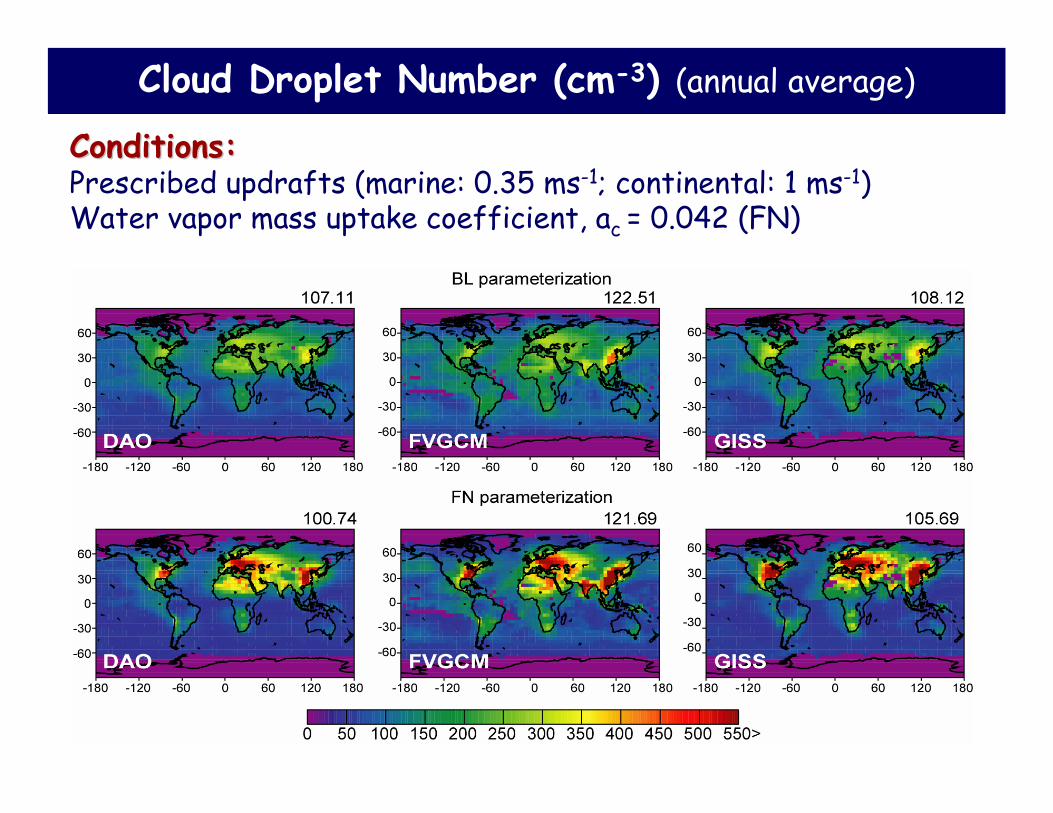
Cloud Droplet Number (cm-3) (annual average)
Conditions:Conditions:Prescribed updrafts (marine: 0.35 ms-1; continental: 1 ms-1)Water vapor mass uptake coefficient, ac = 0.042 (FN)
NS-GISS”
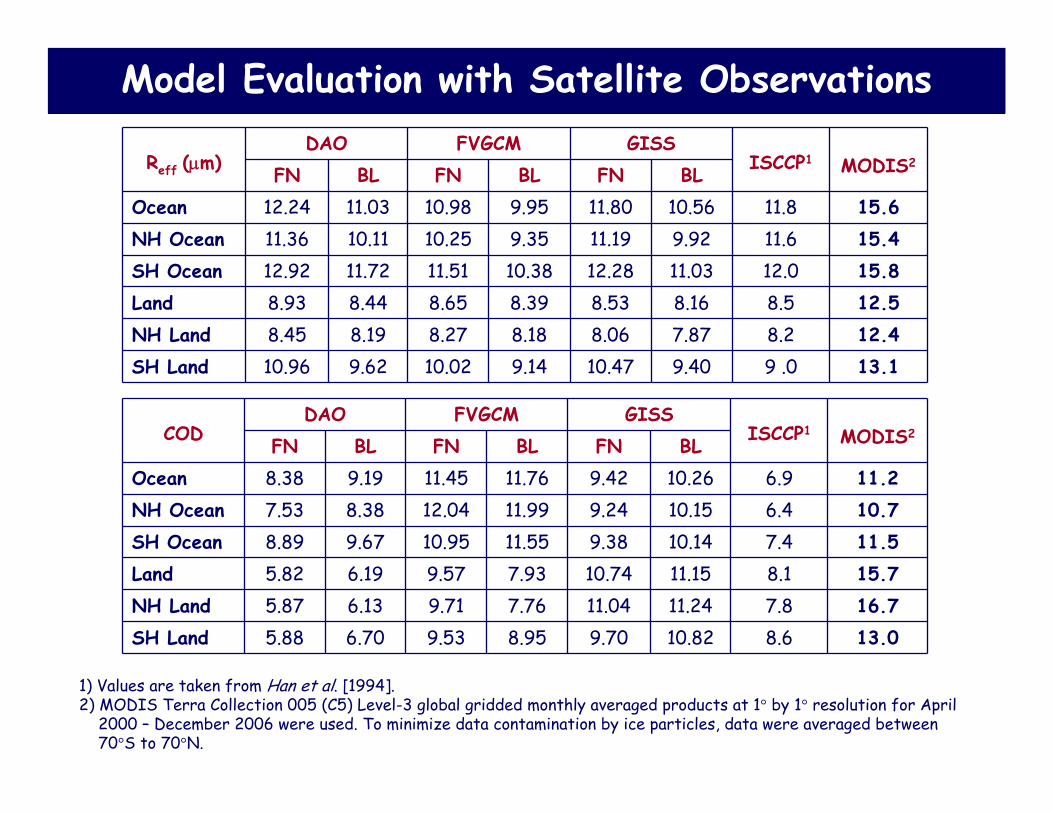
Droplet Effective Radii (μm)
Differences in reffbetween different droplet activation schemes are solely due to differences in predicted CDNC
Satellite and model values agree reasonably well in terms of land-ocean contrast and the differences between SH and NH.
Cloud Optical Thickness ((ττ))
Similar general patterns of COD are predicted for different droplet activation schemes and meteorological fields used.
The modeling results are comparable with those retrieved from MODIS platform
1) Values are taken from Han et al. [1994].2) MODIS Terra Collection 005 (C5) Level-3 global gridded monthly averaged products at 1° by 1° resolution for April
2000 – December 2006 were used. To minimize data contamination by ice particles, data were averaged between 70°S to 70°N.
In the group we also work with the GISS GCM with online aerosol; both mass-based only (Sotiropoulou et al., 2007) and with TOMAS microphysics (Adams and Seinfeld, 2002).
It is important to see how well the GMI simulation, with offline GISS metfields, compares to the GISS climate model simulation with online aerosol (both are run with fixed SST’s and reproduce the general climatology).
Annual Mean First IndirectAnnual Mean First Indirect Forcing (W mForcing (W m--22))
The spatial patterns of indirect forcing follow that of CDNC
Range: -0.99 to -1.48 Wm-2
Annual Mean Autoconversion Rate (Annual Mean Autoconversion Rate (××10101111 ss--11))
Spatial patterns anticorrelated with CDNCSpatial patterns anticorrelated with CDNCAutoconversion much more sensitive to parameterization than AIFAutoconversion much more sensitive to parameterization than AIF
Conditions: Conditions: Eq.1 of KharoutdinovEq.1 of Kharoutdinov and Kogan, 2000and Kogan, 2000
More (interesting) results:“Sensitivity” Simulations
(i.e., Change Liquid Cloud Temperature Threshold, more droplet schemes.)
FVGCM DAO
GISS”
Cloud Droplet Number (cm-3) (annual average)
Conditions:Conditions:Prescribed updrafts (marine: 0.35 ms-1; continental: 1 ms-1)Water vapor mass uptake coefficient, ac = 0.042 (FN)
Despite the general similarity in the spatial patterns, there are considerable differences introduced by differentmeteorological fields and droplet activation parameterizations
Droplet Effective Radii (μm)
Maximum droplet size is calculated over the western tropical Pacific warm pool region, where large evaporation associated with large seasurface temperature exists.
The smallest effective radius is calculated over continental regions with enhanced CCN concentration(i.e., eastern China, North America and Western Europe)
Cloud Optical Thickness ((ττ))
Higher COD is predicted for the clouds overanthropogenically influenced regions of eastern China, Europe,eastern US, and some biomass burning regions in South America andWest Africa.
Different metfields contribute 70% variability in globally averaged COD. Results from different cloud droplet activation parameterizationscontribute a variability of 30%
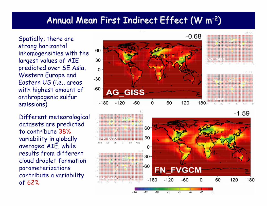
Annual Mean First IndirectAnnual Mean First Indirect Effect (W mEffect (W m--22))
Spatially, there are strong horizontal inhomogeneities with the largest values of AIE predicted over SE Asia, Western Europe and Eastern US (i.e., areas with highest amount of anthropogenic sulfur emissions)
Different meteorological datasets are predicted to contribute 38% variability in globally averaged AIE, whileresults from different cloud droplet formation parameterizationscontribute a variability of 62%
Annual Mean Autoconversion Rate (Annual Mean Autoconversion Rate (××10101111 ss--11))
Conditions: Conditions: Eq.1 of Eq.1 of KharoutdinovKharoutdinov and and Kogan, 2000Kogan, 2000
Different meteorological fields contribute 70 % variability in calculations of autoconversion.
Cloud droplet formation schemes are of lesser importance for autoconversion rate calculations.
The contrast between land and ocean is large.
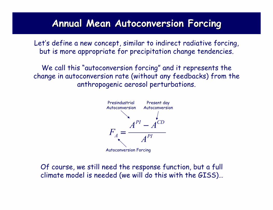
Annual Mean Autoconversion ForcingAnnual Mean Autoconversion Forcing
PI
CDPI
A AAA
F−
=
Present day Autoconversion
Presindustrial Autoconversion
Autoconversion Forcing
Let’s define a new concept, similar to indirect radiative forcing, but is more appropriate for precipitation change tendencies.
We call this “autoconversion forcing” and it represents the change in autoconversion rate (without any feedbacks) from the
anthropogenic aerosol perturbations.
Of course, we still need the response function, but a full climate model is needed (we will do this with the GISS)…
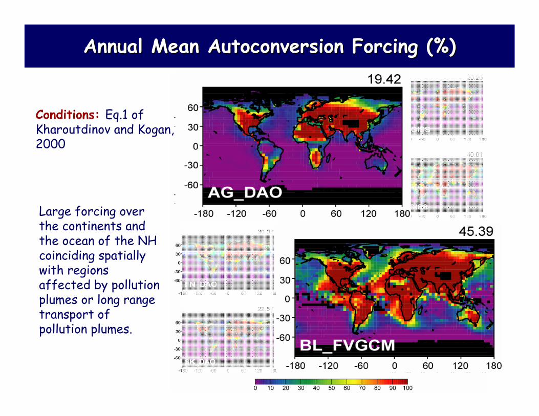
Annual Mean Autoconversion Forcing (%)Annual Mean Autoconversion Forcing (%)
Large forcing over the continents and the ocean of the NH coinciding spatially with regions affected by pollution plumes or long range transport of pollution plumes.
Conditions: Eq.1 of Kharoutdinov and Kogan, 2000
Difference in Annual Mean Autoconversion Rate Difference in Annual Mean Autoconversion Rate Between BL and the Other SchemesBetween BL and the Other Schemes
PDBL
PDBL
PDi
i AAAA −
=Δ
Present day autoconversion predicted by BL
Present day autoconversion predicted by a
scheme (i.e., AG, FN or SK)
(x 10-11 ) s-1
Similar patterns for all metfields.
Large differences over the oceans; this is one of the most important source of uncertainty from the droplet schemes.
This means in the “red”areas we need to do a much better job in computing autoconversion.
AEROCOM simulationsAEROCOM simulations
Conditions: GISS metfields, FN activation scheme, Liquid cloud temperatures above 263 K over land and 269 K over ocean
Nd reff
COD IFSimilar patterns for all properties with the modeling outputs using the emission inventory of the University of Michigan, FN scheme and GISS metfield.
Computational requirements
• BL_DAO: 1 week • SK_DAO: 1 week + 20 min ☺• AG_DAO: 1 week + 45 min ☺• FN_DAO: 1 week + 60 min ☺
BL_GISS: 3 days, BL_FVGCM: 6.5 days
This shatters the common GCM dogma that “Mechanistic Parameterizations (FN) are too slow
to be implemented in GCMs”
Implications and Conclusions• GMI is able to correctly capture the land-ocean
contrast in COD and reff and the spatial variations in cloud properties between the SH and the NH regions observed in remotely sensed data.
• The GMI aerosol simulation with offline GISS winds remarkably reproduces the characteristics of the online GISS (mass-only aerosol simulation).
• Depending on the droplet activation parameterization and the metfield used, global annual indirect forcing ranges:
-0.99 to -1.48 W m-2 for the “Base Case”-0.68 to -1.59 W m-2 for all runs considered to date
• Different metfields lead up to 38% (Global average) variability in indirect forcing calculations.
• Diagnostic and empirical parameterizations contribute up to 62% (Global average) variability in indirect forcing. Although important it is a low estimate (it becomes larger if you use interactive microphysics - our experience with CACTUS and CACTUS/TOMAS support this).
• For all droplet activation parameterizations and the metfields used the global annual autoconversion rate ranges from 1.10×10⁻¹¹ to 10.38×10⁻¹¹ s-1 . The metfields contribute 70% variability and 30% is from the activation parameterization.
Implications and Conclusions
• The spatial patterns of autoconversion rate are similar for all metfields.
• Large differences in autoconversion rates over the oceans; this is one of the most important source of uncertainty from the droplet schemes.
• Larger autoconversion forcing (60-100%) is predicted over the anthropogenically perturbed regions of the globe
Implications and Conclusions
Work in Progress – Future Plans• Run the indirect & autoconversion forcing
simulations for interactive aerosol microphysics. (Joyce)
• Use GISS-TOMAS to extract look-up tables (monthly averages) of the aerosol size distribution and standard deviation as a function of time and place and use them in GMI to calculate indirect & autoconversion forcing.
• Introduce the entraining cloud droplet formation parameterization that we have developed in the group (Barahona and Nenes, JGR, in press)
• “Tie” autoconversion with cloud droplet formation even better.
Work in Progress – Future Plans• Cloud spectrum parameterization (Hsieh and Nenes, in
prep) to link autoconversion with activation; reduce the need for “tuning” autoconversion parameterizations.
• Examine the potential effect of organic compounds on CCN formation (using the “insoluble” fraction of the aerosol).
• Assess the uncertainty in cloud droplet number, indirect radiative forcing and autoconversion rate associated with application of Köhler theory.
• Explicit calculation of the effective radius and the indirect forcing from “k” – Examine the sensitivity to met-fields and droplet formation parameterizations.
• … and the list goes on.
Ongoing projects in the group of potential interest to GMI
(Jose, can we have a few more minutes?)
Procedure:• Use in-situ data and assess CCN closure, for various assumptions on chemical composition taken in GCMs.
• Quantify CCN prediction error
• Incorporate into GCM and assess uncertainty in Cloud droplet number concentration (CDNC)Aerosol indirect forcingAutoconversion of cloudwater to rain
Determine regions where uncertainty is small; define regions where more in-situ constraints are needed.
Assess the indirect forcing uncertainty Assess the indirect forcing uncertainty arising from application of Karising from application of Kööhler theoryhler theory
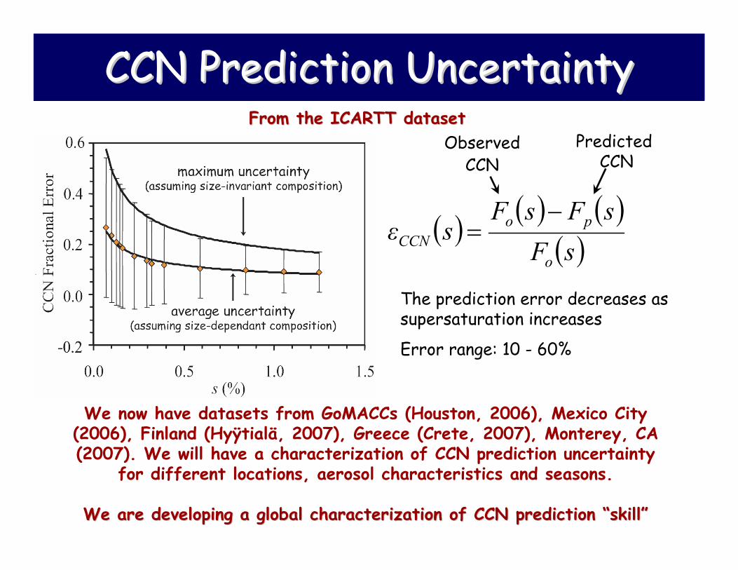
The prediction error decreases as supersaturation increases
Error range: 10 - 60%
From the ICARTT datasetFrom the ICARTT dataset
We now have datasets from GoMACCs (Houston, 2006), Mexico City (2006), Finland (Hyÿtialä, 2007), Greece (Crete, 2007), Monterey, CA (2007). We will have a characterization of CCN prediction uncertainty
for different locations, aerosol characteristics and seasons.
We are developing a global characterization of CCN prediction We are developing a global characterization of CCN prediction ““skillskill””
( ) ( ) ( )( )sF
sFsFsε
o
poCCN
−=
Observed CCN
Predicted CCN
Indirect Forcing Uncertainty
−+
−= maxTOA
maxTOAIF CFCFU
Larger uncertainty is predicted downwind of industrialized and
biomass burning regions
The least indirect forcing uncertainty is predicted over deserts and the subtropical
southern oceans
Global average: 50%
120%806040200
Using the ICARTT dataset in online GISS (Sotiropoulou et al., inUsing the ICARTT dataset in online GISS (Sotiropoulou et al., in press)press)
Range: 10-120%
It would be IDEAL to repeat this within the GMI for different It would be IDEAL to repeat this within the GMI for different met fields, droplet schemes and of course, with all the CCN met fields, droplet schemes and of course, with all the CCN
data at hand! data at hand!
ISORROPIAISORROPIA--II: A new thermodynamic II: A new thermodynamic equilibrium model forequilibrium model for KK++/Ca/Ca2+2+/Mg/Mg2+2+/NH/NH44
++/Na/Na++/ / SOSO44
22--/NO/NO33--/Cl/Cl--/H/H22O AerosolO Aerosol
- Solve the full thermodynamic partitioning equations for aerosol systems with the major inorganic precursors.
- Predict aerosol phase(s), composition of each, and of course, water uptake.
- NASA GISS Global Climate Model- EPA Community Air Quality model
(CMAQ)- EPRI’s CAMx model- Sonoma Tech’s UAM-AERO
- Meteo-France Group- Max Planck Institute for
Tropospheric Research- University of Athens, Greece- Ford Motors - Aachen
New Ice Nucleation Parameterization• Currently looking at
homogeneous freezing
• Freezing of supercooled droplets, influenced by:– Thermodynamical
and dynamical state: (RHi, T, P, updraft velocity)
– Composition and size: their role is still not well understood
• Stochastic process• Very rapid• Proceeds even after
Smax has been surpassed
sice
Nice(cm-3)
Pf
smax
time (s)Example: parcel model simulation of cirus cloud formation. To=233 K, P=340 hPa, W=0.2 ms-1
Barahona D. and Nenes A.,2007, in preparation.
Parameterizing Ice Formation• For each ice particle we trace back its growth and find the
Si at which the freezing occurred, then we calculate nc(Dp, Si)
Freezing Growing
• We look for an asymptotic value of Ni rather than its value at Smax
• Based on first principles; avoid “artificial” constants (i.e., freezing time scales or constant freezing thresholds)
⎟⎟⎠
⎞⎜⎜⎝
⎛⎥⎦
⎤⎢⎣
⎡−
−−=)1(
*)(1max
22max
'
SGwDDSS opo
α )(*)()( ''o
p
foapc s
dDdPsnDn =
Parameterization: Homogeneous Nucleation
( ) ⎥⎦
⎤⎢⎣
⎡−
−
⎟⎟⎠
⎞⎜⎜⎝
⎛−
=2
max
2/3
maxmax
)1()(exp2)(
4
)1()(
oa
ic
DSG
wTkTk
SGwTkS
Nαπ
ρπρβ
α
Parcel Model
Karcher and Lohmann (2002)
This Work
w (ms-1)
Nc (cm-3)
Barahona D. and Nenes A.,2007, in preparation.
Example: To=233 K, P=220 hPa, W=0.2 ms-1
Thank you!
Supporting Material
Cloud Droplet Number (cm-3) (annual average)
Conditions:Conditions:Prescribed updrafts (marine: 0.25 ms-1; continental: 0.5 ms-1)Water vapor mass uptake coefficient, ac, is set to 0.06Bulk microphysics
BLNS
Cloud Droplet Number (cm-3) (annual average)
Conditions:Conditions:Prescribed updrafts (marine: 0.25 ms-1; continental: 0.5 ms-1)Water vapor mass uptake coefficient, ac, is set to 0.06Detailed microphysics (CACTUS/TOMAS)
BLNS
Precipitation formation in GCMs is often decoupled from activation, and generation of rainwater is expressed in terms of a 'critical' liquid water content beyond which rainwater production becomes efficient:
This is not how it happens in nature; rain is a collection process and must be treated as such, if possible.
( ) lAw
lTPl qPc
cCqcq
⎟⎟⎟
⎠
⎞
⎜⎜⎜
⎝
⎛+
⎥⎥
⎦
⎤
⎢⎢
⎣
⎡
⎪⎭
⎪⎬⎫
⎪⎩
⎪⎨⎧
⎟⎟⎠
⎞⎜⎜⎝
⎛−−−=
2/exp1&
(Rotstayn, 1997)
critical LWC for rainwater
conversion rate 'constants'
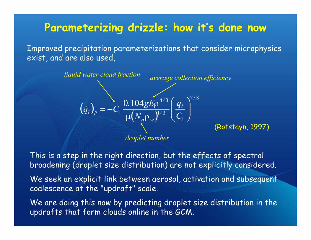
Parameterizing drizzle: how it’s done now
Improved precipitation parameterizations that consider microphysics exist, and are also used,
This is a step in the right direction, but the effects of spectral broadening (droplet size distribution) are not explicitly considered.
We seek an explicit link between aerosol, activation and subsequent coalescence at the "updraft" scale.
We are doing this now by predicting droplet size distribution in the updrafts that form clouds online in the GCM.
(Rotstayn, 1997)
( ) ( )
37
131
34
11040
/
l/
wd
/
Pl Cq
NgE.Cq ⎟⎟
⎠
⎞⎜⎜⎝
⎛−=
ρμρ
&
droplet number
liquid water cloud fraction average collection efficiency
Parameterizing drizzle: how it’s done now
Two-moment schemes developed for small-scale models can be used instead:
Parameterizing drizzle: what we will implement
We have all the elements we need (dispersion, droplet size) for a comprehensive treatment of precipitation. Why not include it in the GCM?
Challenge: How do we obtain these parameters in the global model?
Solution: From the Nenes and Seinfeld Activation Parameterization
(e.g., Cohard and Pinty, 2000; there are more like R4 and R6 schemes of Liu & Daum)
( )( ) 16
3202
5.7105.07.3
4.010161107.2
−
−−
−×
⎟⎠⎞
⎜⎝⎛ −××
−=σ
ρ
σρ
c
vc
Pl
q
Dqq&
spectral dispersionaverage droplet size
Predict size distribution with Nenes and Seinfeld parameterization and cloud parcel model for adiabatic cases of CRYSTAL-FACE (cumulus) clouds.
Use droplet number & size distribution to predict autoconversion rate.
Use in-situ data to calculate autoconversion as well.
The parameterization (and parcel model) capture the spectral width for adiabatic clouds well.
The first parameterization of its kind.Complex organics can be treated, same conceptual framework(“population splitting”) as the adiabatic parameterization. Mixing is parameterized in terms of an entrainment rate.Versions for lognormal and sectional aerosol developed.Same CPU requirements as the adiabatic “version”.
We’ve looked at 4000 casesAverage error:10%
We plan to use CRYSTAL-FACE, CSTRIPE, ICARTT, MASE,
TEXAS-AQS data to constrain the entrainment rate.
The predicted in-cloud dropletsize distribution will be evaluated
with the same dataset.
New cloud droplet formation parameterization(Includes entrainment)
Why need a new parameterization?• Current parameterizations are adiabatic. Clouds are generally not. • Droplet number predictions are good even for slightly diabatic conditions
(although Nd can still be overestimated for strong entrainment).• Nenes and Seinfeld can predict droplet size distribution, but they are too
narrow (adiabatic), so autoconversion calculations would generally be “off”.
• Comparison of predicted size distribution “width” vs. liquid water content for non-adiabatic CRYSTAL-FACE (cumulus) clouds.
• Parameterization and cloud parcel model agree great with each other, but not with the data (even though cloud droplet number is captured to within 5%!).
• An entraining parameterization would improve this because entrainment broadens the distribution.
• Droplets freeze in groups at the same supersaturation, so’, and grow defining the crystal size distribution, nc(s, Dp)• The fraction of frozen droplets is determined by the
probability of freezing Pf (so’ )
Supercooled Droplets
Ice Crystals
Freezing
Growing
)( pc D,sn
)( oo D,sn
oaia
waiestice ss
Gw
MpMpN *01.14 2
0 =⎟⎠⎞
⎜⎝⎛=α
πρρ
610?/
exp1)( −≤⎟⎠⎞
⎜⎝⎛−−= ∫
SCo
f dsdtds
JvsP
estcC
oaice Nds
dsDsdPnN
S
?),(== ∫
yesNo
Ncest= Nc
Increase s
Initial guesses
Correct Nc
Correct s
Output: Nc, s
yes
No
Parameterization Algorithm
We count the number of crystals, Nice, until some supersaturation, s,is reached at which the freezing pulse is over
time
Sice
sso
Pf
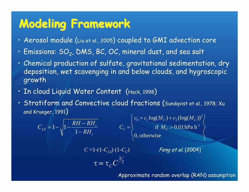
Modeling FrameworkModeling Framework• Aerosol module (Liu et al., 2005) coupled to GMI advection core• Emissions: SO2, DMS, BC, OC, mineral dust, and sea salt• Chemical production of sulfate, gravitational sedimentation, dry
deposition, wet scavenging in and below clouds, and hygroscopic growth
• In cloud Liquid Water Content (Hack, 1998)• Stratiform and Convective cloud fractions (Sundqvist et al., 1978; Xu