CHARLES UNIVERSITY IN PRAGUEFACULTY OF SOCIAL SCIENCES

Institute of Economic Studies

Kratochvıl Maxim, Nedved Adam, Papousek Radan

Forecasting the household consumptionof the Czech Republic using the model

based on data from search engines

JEM004 Advanced Macroeconomics

Prague 2015

Contents

1 Introduction 2

2 Literature review 4

2.1 Sentiment indicators and their use in consumption forecasting . . . . 4

2.2 Predicting with Google Trends . . . . . . . . . . . . . . . . . . . . . . 6

3 Data & Model 10

3.1 Data . . . . . . . . . . . . . . . . . . . . . . . . . . . . . . . . . . . . 10

3.1.1 Czech sentiment indicators and household consumption in the

Czech Republic . . . . . . . . . . . . . . . . . . . . . . . . . . 10

3.1.2 Data originating from Google Trends . . . . . . . . . . . . . . 12

3.2 Model . . . . . . . . . . . . . . . . . . . . . . . . . . . . . . . . . . . 14

4 Results 16

5 Conclusion 18

Bibliography 19

Appendix A 21

1

Chapter 1

Introduction

Consumption is one of the key concept in economics. It greatly influences other

macroeconomic variables such as import or investments. Since consumption is one

of the main determinants of country’s GDP, it has a direct effect on economic per-

formance of a given country. According to Eurostat, share of private consumption

on EU’s GDP was ca. 57 % in 2014. Many well-known theories were developed

in order to describe and explain dependencies between consumption and other eco-

nomic variables (e.g. disposable income, current wealth). For instance, consumption

plays one of the central role in Keynesian economics, but there is no unified view on

how consumption level is determined. Friedman and Modigliani developed different

mechanisms how households decide about their consumption. Nowadays, behavioral

economics and microeconomics try to explain it. Recent development in technology

gives us other estimation tools. One of the tools, which has gained quite a lot of

attention, is Google Trends or so-called Google econometrics.

Since consumption plays a major role in many macroeconomic models and thus in

forecasting future economic development, profound and accurate estimation method

of consumption expenditure is crucial. Moreover, household consumption is in a

direct connection with quality of life of individuals. People often interchange eco-

nomic performance of their country and their personal consumption. Dynamics

of consumption is closely monitored and can even influence elections on country

2

CHAPTER 1. INTRODUCTION 3

level and overall sentiment in the economy. As recent research shows prediction of

consumption can be quite accurate, when Google Trends are employed (inter alia,

Schmidt & Vosen (2009), Schmidt & Vosen (2010), Toth & Hajdu (2013). We ex-

amine accurateness of predictions of consumption in the Czech Republic based on

Google Trends, and provide the comparison with the accuracy of the Czech Sta-

tistical office’s predictions and baseline model, where only explanatory variable is

lagged consumption. Due to small sample size, we perform bootstrap estimation to

enhance our forecast analysis. Then we compare RMSEs of the individual models.

The paper is structured in the following way: next section briefly summarizes

existing literature. Section 3 introduces data and the model. Section 4 reports

results, and section 5 concludes.

Chapter 2

Literature review

In this section, we discuss consumer confidence indices and their possible benefits

for consumption forecasting. Further, we review recent development in research

employing Google Trends.

2.1 Sentiment indicators and their use in con-

sumption forecasting

We use the definition of household consumption as it is defined by the World Bank

(2015): “...the market value of all goods and services, including durable products

(such as cars, washing machines, and home computers), purchased by households.”

There exists an extensive research about consumption and ways of its forecast-

ing. Estimation based on sentiment indicators is one of the most common, because

such data are easily available (Schmidt & Vosen 2010). They are extracted from

household surveys, which are usually collected on a monthly or a quarterly basis.

Consumer confidence indices are closely monitored macroeconomic variables. Policy

makers analyze them when deciding about monetary policy and are also heavily used

by other participants on the market such as investors or economists. Hall (1993)

stresses how crucial accurate estimation of future household consumption is; the

4

CHAPTER 2. LITERATURE REVIEW 5

author pinpoints that decrease in consumption can be one of the triggers of eco-

nomic recessions. Nevertheless, researches argue whether there is some information

about future consumption in the indicators, which is not already in macroeconomic

variables such as income, wealth, or real interest rate. Mehra & Martin (2003) con-

clude that the sentiment indicators have predictive value in estimating near-term

consumption and that they foreshadow contemporary economic situation. In influ-

ential paper, Carroll et al. (1991) suggest two distinct interpretations why sentiment

indicators have predictive power

1. the indicators are independent determinants of consumption,

2. the indicators foreshadows current economic conditions.

Easaw et al. (2005) find that when forecasting total consumption in the UK, the

consumer confidence indices have very low additional informational value; nonethe-

less when focusing only on durable goods, they prove that the indicators carry some

information, which is not already incorporated in other economical and financial

variables. Easaw et al. (2005) further claim that such indicators can be good pre-

dictors of future consumption up to 4 quarters for total consumption and up to 1

quarter for consumption of durable goods. Similar, but weaker, results hold for the

US.

Croushore (2004) admits that sentiment indicators are strongly correlated with

future household consumption, but he fails to find any significant value in the indi-

cators regarding future consumption other than the one which is already embodied

in different variables. He further argues that much research is conducted on flawed

data. The author criticizes such literature that it uses revised data, which could

not be available to the forecasters at that time. Therefore any conclusion drawn

from such research may not be correct. The author even states that employing non-

revised consumer confidence indices may actually worsen consumption forecasts in

certain cases. Further, Vuchelen (2004) declares that since mechanism behind con-

sumer sentiment is not well explored, employing such variable in a forecast model

CHAPTER 2. LITERATURE REVIEW 6

may be troublesome.

Vuchelen (2004) divides research on consumption forecast using sentiment indi-

cators into two groups. The first group claims that “consumer sentiment reflects

not only economic conditions but, more broadly, the subjective state of mind of

consumers” (Vuchelen 2004, p.495). Due to the complexity of human behavior,

economic variables are not able to capture the whole information in consumer senti-

ment, thus the indicators possess some kind of information that can be used (Vuche-

len 2004). The hypothesis that the amount of information the indicators hold may

vary over time was refused by Katona (1976), he found that due to mass media

and personal communication the relationship is relatively stable. The second group

claims that consumer confidence indicators have no own informational value. They

just capture households’ expectation about future and such expectations can be well

explained by other economic variables.

2.2 Predicting with Google Trends

The essential part of our project is to demonstrate that methodology suggested is

working with useful data, so it would be clear that its usage has proper validity and

reasoning. To do so, we examine existing literature that describes similar concept

of research.

Main tools used by macroeconomy theorists to forecast private consumption are

basic macroeconomic variables and survey-based research that tries to substitute

the hidden psychology effects that are consumers driven by. To be more specific,

macroeconomic variables describe simply the ability to spend and surveys are often

focused on the willingness to spend. Such data are still obviously very insufficient

in order to obtain solid knowledge-base for consumption forecasting.

The main motivation to work with Google Trends is based on the idea, that

although the share of the online retail sales is estimated at only about 3.5% in

the US, it is expected that the vast majority of consumers is also Internet users

CHAPTER 2. LITERATURE REVIEW 7

and they ’consult’ their decision with the online offers and supply. According to

eMarketers (agency focusing on the US market), 86% of the Internet users are also

online shoppers. If those two facts are combined, eMarketers estimate that store sales

are influenced by online research three times more than e-commerce sales, just due

to the possibility of online cross-market comparison that is available to consumers

(Schmidt & Vosen 2009). To sum up the main idea, if there are data that contain

some information about search queries and behaviors of consumers online, we expect

that such data could be linked to actual trends in private consumption and therefore

to simulate some short-time forecasts.

Although the Google Trends (or Google Insight as it was called in the past)

data have been publicly available since 2008, first usage of similar method using top

searched keywords (published by company called Rivergold Associates) for forecast-

ing purposes was documented in 2005, applied on the examination of unemployment

rate in the US (Choi & Varian 2012).First breakthrough in usage of Google Trends

was made by Choi & Varian (2009) examining the data for retail sales and automo-

tive sales in the US. Since then, there have been many other studies and papers using

Google Trends, covering for example epidemiology, inflation, vacation destination,

and many other topics.

Reading through many sources, it is important to mention that Google Trends

provide rather short-term predictions or so-called ’nowcasting’, covering few weeks

at maximum. It is worth to mention that models with or without Google data

provide almost identical results during the average/normal time periods, however,

during the time periods with some sudden changes or shocks in the economy, models

using Google data outperform the basic models (Kholodilin et al. 2009).

The paper by Choi & Varian (2012) has served mostly like a manual for other

researchers. Their work provided another proof that models which employ Google

Trends outperform basic models by 5 % to 20 %.

To provide a short example of setting up the model using Google Trends, let us

CHAPTER 2. LITERATURE REVIEW 8

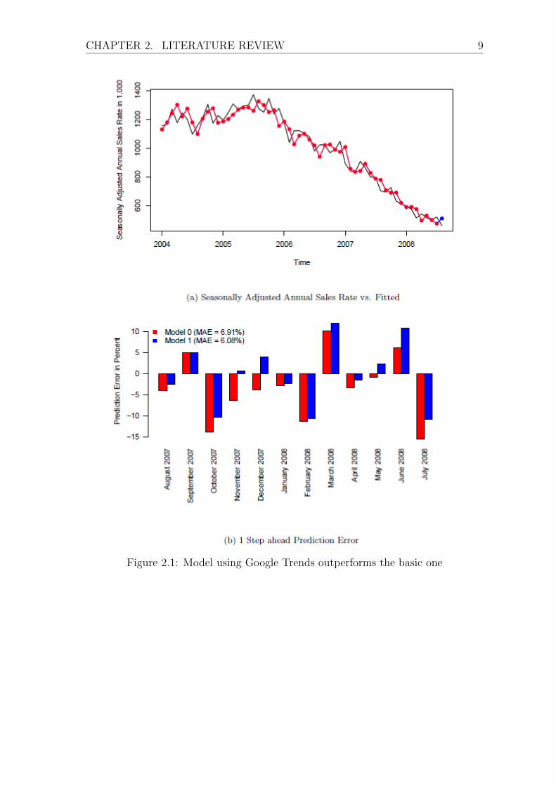
use one of the model used by Choi & Varian (2009) forecasting the home sales. First

of all, the authors examine data published by the US Statistical Offices. Secondly,

the authors found all search indexes that may play role in regards of the examined

topic. In this example, they found 6 searched keywords from the Google Trends

data pool, those were: Real Estate Agencies, Rental Listings & Referrals, Property

Management, Home Inspections & Appraisal, Home Insurance and Home Financing.

Model is then fitted for seasonally adjusted sales figures and its equation (so far

without Google Trends data) is following:

log(yt) ∼ log(yt−1) + et (2.1)

, where et represents the error term. When the additional exogenous variables

were plugged in, estimates of the model show that search index Rental Listings &

Referrals is negatively related to house sales and search index Real Estate Agencies is

positively related. Other indexes were insignificant. To briefly present the summary

of the results, model using Google Trends data provided estimates with 12% lower

mean absolute error (MAE) in terms of one-step ahead prediction errors. The graph

for Seasonally Adjusted Sales Rate vs. Fitted values and One-Step Ahead Prediction

Errors could be seen in Figure 2.1.

Although the research in econometrics using search indexes lasts only for a short

period of time, existing literature provides strong examples of validity of such models

with remarkable results.

CHAPTER 2. LITERATURE REVIEW 9

Figure 2.1: Model using Google Trends outperforms the basic one

Chapter 3

Data & Model

This section describes the data employed in the model and introduces the model

itself.

3.1 Data

3.1.1 Czech sentiment indicators and household consump-

tion in the Czech Republic

The Czech Statistical Office (abbreviated as CZSO) estimates the consumer sen-

timent by simple surveys. According to CZSO (2015), surveys are aimed to capture

households’ expectations about the near-term future (1 month, 3 months, and 6

months forward). Their structure is rather simple; for illustration, we provide one

of the questions from business confidence survey: “Expected orders (contracts) for

the next 3 months:

1. will increase

2. will not change

3. will decrease”

10

CHAPTER 3. DATA & MODEL 11

(CZSO 2015, para.3). The results are then presented as business cycle balance,

“which is the difference between the answers ’improvement’ and ’worsening’ ex-

pressed in percents. The higher the positive balance of answers the more optimistic

is the evaluation of the answer obtained” (CZSO 2015, para.4). The survey method-

ology is coordinated and harmonized with respect to the European Commission and

OECD. The consumer confidence indicator consists of 4 elements:

1. “expected financial situation of consumers

2. expected total economic situation

3. expected total unemployment (with inverted sign)

4. savings expect in 12 months to come”

(CZSO 2015, para.9). Surveys are conducted on a monthly basis.

CZSO provides data for consumption of Czech households on a quarterly ba-

sis. The pool of households that is selected for a given time period is chosen to

represent average structure of households of the Czech Republic. Data in sufficient

quality are available since 2010. The structure of data provided by CZSO has several

subcategories and its fragmentation is following:

i) total income of household, divided by type of household (number of working

persons, of unemployed persons, of children, no children in household) and the origin

of the income (employment, social system support, entrepreneurship) in %,

ii) total spending of household divided by the same groups as in category i). De-

tailed structure of spendings in categories (e.g. alcohol, tobacco, clothes, education,

culture, etc.) is available,

iii) indexed structure of spendings with reference to spendings a year before

given survey.

These data could be also structured according to the size of the municipality

that household lives in and according to the type of ownership of the real estate

that household occupies (owns a family house, pays rent for a flat, etc.)

CHAPTER 3. DATA & MODEL 12

With focus on our research, specific fragmentation of household spendings is

not as important. It could be beneficial only with change of the focus to some

particular category. Our priority is the total household spending. Since the survey

is worked out only every 3 months, some adjustments and rearrangements will have

to be done in data from Google Trends to fit the format of official statistics. As

mentioned earlier, Google Trends data serve the best when predicting very near

future - nowcasting. Since we conduct research on quarterly based data, we expect

that contribution of Google Trends data would be rather smaller. With higher

frequency in data, contribution of Google Trends is expected to increase.

3.1.2 Data originating from Google Trends

Google Trends is based on searches conducted through Google web search engine.

It shows how frequently is a query submitted relative to the total number of searches

in a specified geographical location and over specified time period. Google launched

such feature in 2008, nevertheless data from Google Trends are available from 2004.

Google adjusts the data to make them easier to compare, so they do not reflect

absolute search volumes, they rather represents popularity of a given search entry.

Figures are scaled to range between 0 and 100. The higher number, the more

popular query. 0 means that the query was not submitted by enough people and

value 100 is assigned to the most popular point in the chosen time series. The data

are published on a weekly basis with almost no lag. It measures popularity of a

given query only in the language of the query. For instance, when showing data for

query ’consumption’, it does not add the data for searches of ’consumption’ in other

languages. Such feature is very convenient for our research, since we focus only on

the Czech Republic. Google Trends groups searched words into categories such as

Home & Garden, or Shopping, so it is easier for researches to use it. Unfortunately,

this feature is not available for the Czech Republic. Our research depends on words

we believe fit our purpose the best - will be discussed in more detail further in the

CHAPTER 3. DATA & MODEL 13

text. Figure 3.1 illustrates how Google Trends works.

Figure 3.1: Google Trends depicting data for consumption, debt, growth, and con-fidence over given time period

List of queries that was used for generating data for variable xi,t is based on the

list published in Platil (2014). The author examines different key words and their

relation to the Czech consumer confidence index, and then picks the most relevant

ones. We also include queries without diacritic - see table 3.1.

We included names of the two Czech largest Internet shops - Alza.cz a.s. and

Internet Mall, a.s. and the biggest price tracker Heureka.cz. Although e-commerce

makes only ca. 9 % of the all retail sales, the industry is growing rapidly. It may

have also secondary effect on consumption. People look merchandise up on the

mentioned websites and then buy it in physical store.

The examined period is from 1Q2008 to 3Q2015.

CHAPTER 3. DATA & MODEL 14

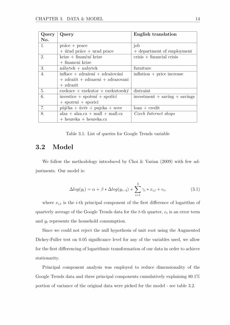
Query Query English translationNo.1. prace + prace job

+ urad prace + urad prace + department of employment2. krize + financnı krize crisis + financial crisis

+ financni krize3. nabytek + nabytek furniture4. inflace + zdrazenı + zdrazovanı inflation + price increase

+ zdrazit + zdrazeni + zdrazovani+ zdrazit

5. exekuce + exekutor + exekutorsky distraint6. investice + sporenı + sporıcı investment + saving + savings

+ sporeni + sporici7. pujcka + uver + pujcka + uver loan + credit8. alza + alza.cz + mall + mall.cz Czech Internet shops

+ heureka + heureka.cz

Table 3.1: List of queries for Google Trends variable

3.2 Model

We follow the methodology introduced by Choi & Varian (2009) with few ad-

justments. Our model is:

∆log(yt) = α + β ∗ ∆log(yt−4) +3∑

i=1

γi ∗ xi,t + et, (3.1)

where xi,t is the i-th principal component of the first difference of logarithm of

quarterly average of the Google Trends data for the t-th quarter, et is an error term

and yt represents the household consumption.

Since we could not reject the null hypothesis of unit root using the Augmented

Dickey-Fuller test on 0.05 significance level for any of the variables used, we allow

for the first differencing of logarithmic transformation of our data in order to achieve

stationarity.

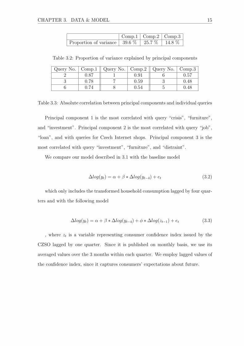
Principal component analysis was employed to reduce dimensionality of the

Google Trends data and three principal components cumulatively explaining 80.1%

portion of variance of the original data were picked for the model - see table 3.2.

CHAPTER 3. DATA & MODEL 15

Comp.1 Comp.2 Comp.3Proportion of variance 39.6 % 25.7 % 14.8 %

Table 3.2: Proportion of variance explained by principal components

Query No. Comp.1 Query No. Comp.2 Query No. Comp.32 0.87 1 0.91 6 0.573 0.78 7 0.59 3 0.486 0.74 8 0.54 5 0.48

Table 3.3: Absolute correlation between principal components and individual queries

Principal component 1 is the most correlated with query “crisis”, “furniture”,

and “investment”. Principal component 2 is the most correlated with query “job”,

“loan”, and with queries for Czech Internet shops. Principal component 3 is the

most correlated with query “investment”, “furniture”, and “distraint”.

We compare our model described in 3.1 with the baseline model

∆log(yt) = α + β ∗ ∆log(yt−4) + et (3.2)

which only includes the transformed household consumption lagged by four quar-

ters and with the following model

∆log(yt) = α + β ∗ ∆log(yt−4) + φ ∗ ∆log(zt−1) + et (3.3)

, where zt is a variable representing consumer confidence index issued by the

CZSO lagged by one quarter. Since it is published on monthly basis, we use its

averaged values over the 3 months within each quarter. We employ lagged values of

the confidence index, since it captures consumers’ expectations about future.

Chapter 4

Results

In order to assess the forecasting ability of the model including the Google Trends

data against the the baseline model and the model including consumer confidence

index, we have performed out of sample forecasting for the period including the last

four quarters in our dataset. Root mean squared error was chosen as a measure

of accuracy. Since our dataset is somehow limited, we have employed the block

bootstrapping method for time series in order to fit all three models. Each of 1000

runs of the bootstrap algorithm was used to obtain OLS fit on the dataset of 27

observations sampled with replacement from all of our available observations by

blocks of four. Each time, the resulting OLS estimates were used to perform out

of sample forecast on the four remaining observations and the resulting root mean

squared error of the forecast was calculated. The means of resulting distributions of

RMSEs are reported in the following table together with 95% confidence intervals

obtained using the quantile method. Histograms of bootstrap estimates of RMSEs

for individual models can be found in Appendix A.

We report the result in the table below.

16

CHAPTER 4. RESULTS 17

Model RMSE SE CI: 2.5 % CI: 97.5 %Baseline 0.029 (0.009) 0.018 0.052

Confidence Index 0.029 (0.010) 0.016 0.052Google Trends 0.018 (0.017) 0.007 0.071

Table 4.1: Bootstrap results for baseline, confidence index, and Google Trends model

The results show that the model based on the consumer confidence index per-

forms worse compared to the Google Trends model in terms of RMSE. It has the

highest value of RMSE together with the baseline model. The model based on

Google Trends data has the lowest value of RMSE; on the other hand, it has also

the highest standard error. Thus while seemingly it is performing the best, we can-

not draw any strong conclusion about its forecast ability. Nevertheless, we show

that Google Trends data contain some information that can be used for household

consumption prediction. As said earlier, with higher frequent data, Google Trends

would be more useful. Instant availability is one of its indisputable advantages.

Chapter 5

Conclusion

We examined forecasting ability of the Google Trends data on Czech household

consumption. Since consumption is one of the key determinants of GDP develop-

ment, its accurate prediction is crucial for any macroeconomic model. We show

that model based on the data from Google Trends can be more efficient compared

to conventional tools such as consumer confidence indicators. We performed forecast

based on bootstrap estimates and compared RMSEs between 3 models: the baseline

model with only one variable - lagged consumption by 4 quarters, the model based

on consumer confidence index, and the model based on the Google Trends data.

Nevertheless, since we conducted research on the data with quarterly frequency,

contribution from the Google data is rather small, since it has the highest standard

error of RMSE among the examined models. When employed with higher frequent

data, contribution is expected to rise. Moreover, the Google trends are readily avail-

able with almost no lag. Since we cannot say which model is better based on RMSEs

and SEs, the feature of instant availability of Google data compared to lagged re-

sults of consumer confidence index, makes the model based on Google data superior

in terms of rough prediction of near consumption development.

18

Bibliography

Carroll, C. D., Fuhrer, J. C. & Wilcox, D. W. (1991), Does consumer sentiment

affect household spending? if so why?, Finance and Economics Discussion Series

168, Board of Governors of the Federal Reserve System (U.S.).

Choi, H. & Varian, H. (2009), Predicting the present with google trends, Technical

report, Google Inc.

Choi, H. & Varian, H. (2012), ‘Predicting the present with google trends’, The

Economic Record 88(s1), 2–9.

Croushore, D. (2004), Do consumer confidence indexes help forecast consumer

spending in real time?, Discussion Paper Series 1: Economic Studies 2004,27,

Deutsche Bundesbank, Research Centre.

CZSO (2015), ‘Business cycle surveys - methodology’, [Online] Available from:

https://www.czso.cz/csu/czso/konjunkturalni pruzkum. [Accesed on 27.11.2015].

Easaw, J. Z., Garratt, D. & Heravi, S. M. (2005), ‘Does consumer sentiment accu-

rately forecast uk household consumption? are there any comparisons to be made

with the us?’, Journal of Macroeconomics 27(3), 517–532.

Hall, R. E. (1993), ‘Macro theory and the recession of 1990-1991’, American Eco-

nomic Review 83(2), 275–79.

Katona, G. (1976), ‘Psychological economics’, Journal of Behavioral Economics

5(1), 203–205. Elsevier Scientific Publishing Company, New York (19).

19

BIBLIOGRAPHY 20

Kholodilin, K. A., Podstawski, M., Siliverstovs, B. & Burgi, C. (2009), Google

searches as a means of improving the nowcasts of key macroeconomic variables,

Discussion Papers of DIW Berlin 946, DIW Berlin, German Institute for Economic

Research.

Mehra, Y. P. & Martin, E. W. (2003), ‘Why does consumer sentiment predict house-

hold spending?’, Economic Quarterly (Fall), 51–67.

Platil, L. (2014), Google econometrics: An application to the czech republic, Mas-

ter’s thesis, Charles University in Prague, Faculty of Social Sciences, Institute of

Economic Studies.

URL: https://is.cuni.cz/webapps/zzp/download/120158583/?lang=cs

Schmidt, T. & Vosen, S. (2009), Forecasting private consumption: Survey-based in-

dicators vs. google trends, Ruhr Economic Papers 0155, Rheinisch-Westfalisches

Institut fur Wirtschaftsforschung, Ruhr-Universitat Bochum, Universitat Dort-

mund, Universitat Duisburg-Essen.

Schmidt, T. & Vosen, S. (2010), A monthly consumption indicator for germany

based on internet search query data, Ruhr Economic Papers 0208, Rheinisch-

Westfalisches Institut fur Wirtschaftsforschung, Ruhr-Universitat Bochum, Uni-

versitat Dortmund, Universitat Duisburg-Essen.

the World Bank (2015), ‘Data’, [Online] Available from:

http://data.worldbank.org/indicator/NE.CON.PETC.ZS. [Accesed on

27.11.2015].

Toth, I. J. & Hajdu, M. (2013), Google as a tool for nowcasting household consump-

tion: estimations on hungarian data, Technical report, Institute for Eonomic and

Enterprise Research - HCCI.

Vuchelen, J. (2004), ‘Consumer sentiment and macroeconomic forecasts’, Journal of

Economic Psychology 25(4), 493–506.

Appendix A

Table A.1: Bootstrap estimates of RMSEs for the baseline model

0

20

40

0.025 0.050 0.075Root Mean Squared Error, Bootstrap Est. (R = 1000, 95% CI)

dens

ity

Baseline

Table A.2: Bootstrap estimates of RMSEs for the model based on the consumerconfidence index

0

10

20

30

40

50

0.025 0.050 0.075Root Mean Squared Error, Bootstrap Est. (R = 1000, 95% CI)

dens

ity

Confidence Index

21

APPENDIX A. 22

Table A.3: Bootstrap estimates of RMSEs for the model based on the Google Trendsdata

0

10

20

30

0.000 0.025 0.050 0.075 0.100Root Mean Squared Error, Bootstrap Est. (R = 1000, 95% CI)

dens

ity

Google Trends