Gromacs Workshop Spring 2007 @ CSCErik LindahlCenter for Biomembrane ResearchStockholm University, Sweden

David van der SpoelDept. Cell & Molecular BiologyUppsala University, Sweden

Berk HessMax-Planck-Institut for Polymer ResearchMainz, Germany For CSC: Atte Sillanpää

lindahl@cbr.su.selindahl@gromacs.org

CBR

Introduction to Molecular Simulation

and Gromacs

Erik Lindahl

Outline: Introduction• Why and when are simulations useful?

• Various approaches, approximations

• Things we can (and cannot) model

• Time and length scales accessible

• Interactions, equations of motion

• Periodic boundary conditions & cells

• Ensembles: temperature, pressure, etc.

• When can you trust the results?

Why Simulations?

• Test models

• Test theories

• “atomic microscope”

• Way too many simulationsare performed without anyhypothesis / clear plan

• Think first, then simulate!

Allen & Tildesley

Molecular Modeling• The art of describing complex chemical

systems from atomic/quantum models

• Prediction of macroscopic properties

• Ensemble averages

• Static / Equilibrium properties

• Dynamic / Non-equilibrium properties

• Everything described by Schrödinger:

H!(x, t) = E!(x, t)

Timescales

Simulations

Extreme detail

Sampling issues?

Parameter quality?

Experiments

Efficient averaging

Less detail

s -3 0-6-15 -12 -9 310 10 10 10 10 10 10s s s s s sWhere we are

Where we

want to be

Where we

need to be

Limitations of QM

• QM is necessary to describe electronic, and sometimes hydrogen, motion

• Heavy atoms can be treated classically

• Can only solve up to ~100 atoms accurately

• No time dependence

• Several approximations exist, but they are only accurate on QM scale - you cannot extrapolate 10 orders of magnitude!

Empirical models

• Classical particles

• Parameterize to reproduce experiments

• Some properties like charge, bond parameters can be obtained from QM(Semi-empirical models)

• Atomic simulation is not always the best choice

• coarse-grained methods (Marrink)

• QSAR, chemoinformatics

Example properties

• Free energy (of binding, solvation, interaction)

• Diffusion coefficients, viscosity

• Reaction rates, phase transition properties

• Protein folding times

• Structure refinement

• All of these are ensemble averages over huge numbers of molecules (Navogadro ~6E23)

Example properties• Free energy (of binding, solvation, interaction)

• Diffusion coefficients

• Reaction rates

• Protein folding times

• Structure refinement

• All of these are ensemble averages of many molecules (Navogadro ~6E23)

• Thus, our goal is to sample equilibrium ensembles, not simulate individual particles!

Sampling methods

• Monte Carlo simulation

• No time dependence

• Requires intelligent moves

• Newton’s equations of motion

• Time dependence

• Dynamical events

• Stochastic / Brownian dynamics

• Add noise to forces

Energy landscapes

• 3N-dimensional space

• Native structure is the free energy minimum

• Ideally, we would sample all of phase space exhaustively

• In practice we have to make do with the most populated parts

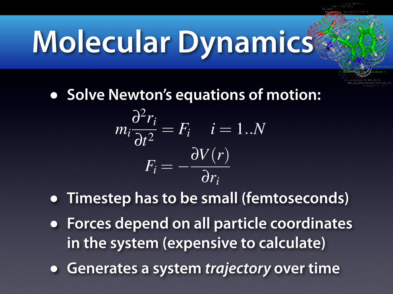
Molecular Dynamics

• Solve Newton’s equations of motion:

• Timestep has to be small (femtoseconds)

• Forces depend on all particle coordinates in the system (expensive to calculate)

• Generates a system trajectory over time

mi!2ri

!t2 = Fi i = 1..N

Fi =!!V (r)

!ri

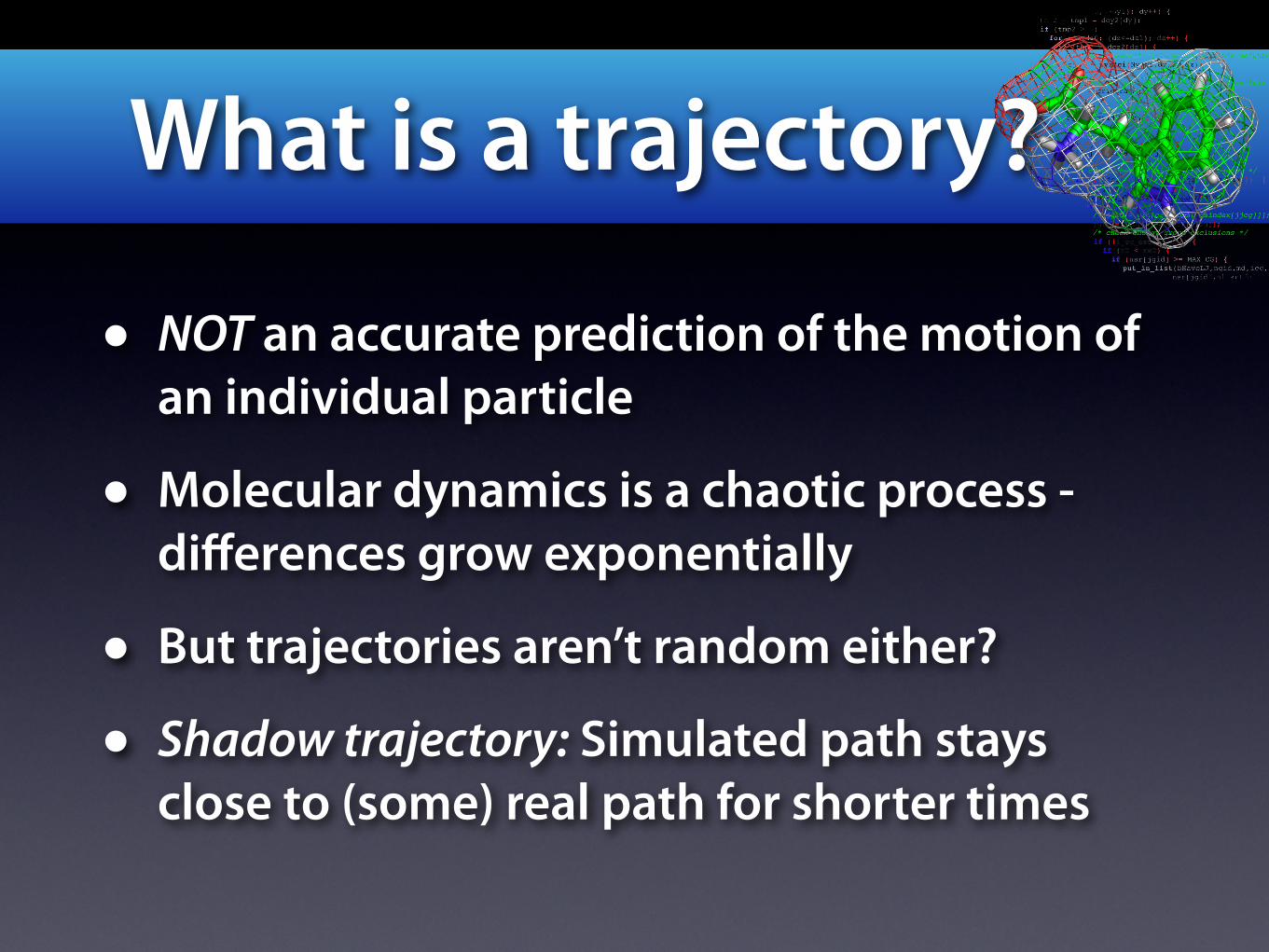
What is a trajectory?

• NOT an accurate prediction of the motion of an individual particle

• Molecular dynamics is a chaotic process - differences grow exponentially

• But trajectories aren’t random either?

• Shadow trajectory: Simulated path stays close to (some) real path for shorter times

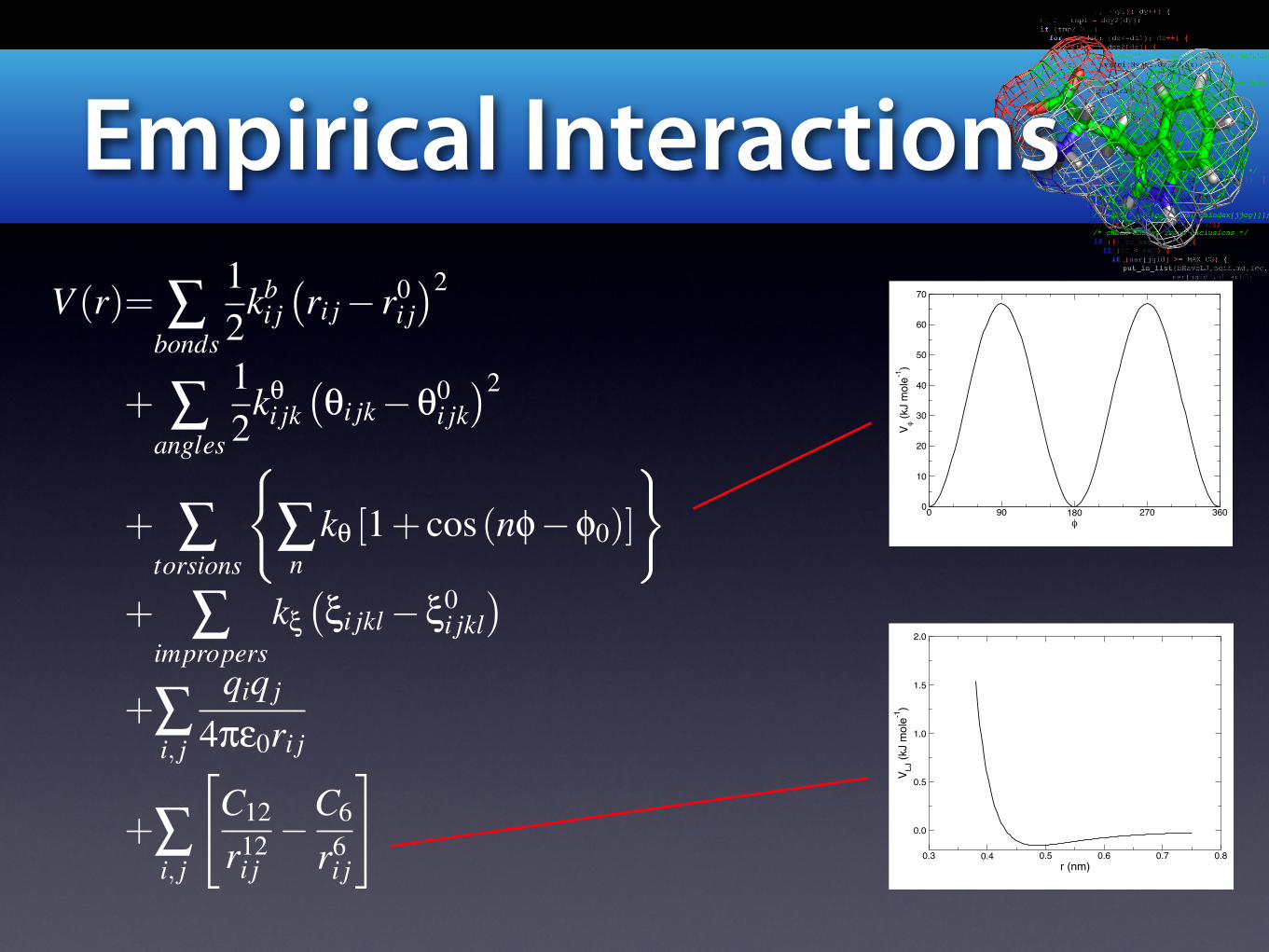
Empirical Interactions

Empirical Interactions

0.3 0.4 0.5 0.6 0.7 0.8

r (nm)

0.0

0.5

1.0

1.5

2.0

VL

J (

kJ m

ole

-1)

0 90 180 270 360

!

0

10

20

30

40

50

60

70

V! (

kJ m

ole

-1)

V (r)= !bonds

12

kbi j!ri j! r0

i j"2

+ !angles

12

k"i jk

!"i jk!"0

i jk"2

+ !torsions

#

!n

k" [1+ cos(n#!#0)]

$

+ !impropers

k$!$i jkl!$0

i jkl"

+!i, j

qiq j

4%&0ri j

+!i, j

%C12

r12i j!C6

r6i j

&

Taking a timestep

10 ps!

Environments

Unrealistic Realistic

Boundary conditions

• Vacuum: No solvent

• Droplet: Spherical layer of water around protein, solvent molecules constrained with random forces (not in Gromacs)

• Periodic Boundary Conditions (PBC) - a water that exits on the right reappears on the left

Periodic cell shapes

• Cubic / rectangular

• Truncated octahedron (more spherical)

• Rhombic dodecahedron(most spherical cell)

• Octahedron volume is only 77% of cube, and dodecahedron 71% at same periodic distance!

Truncatedoctahedron

Rhombic dodecahedron

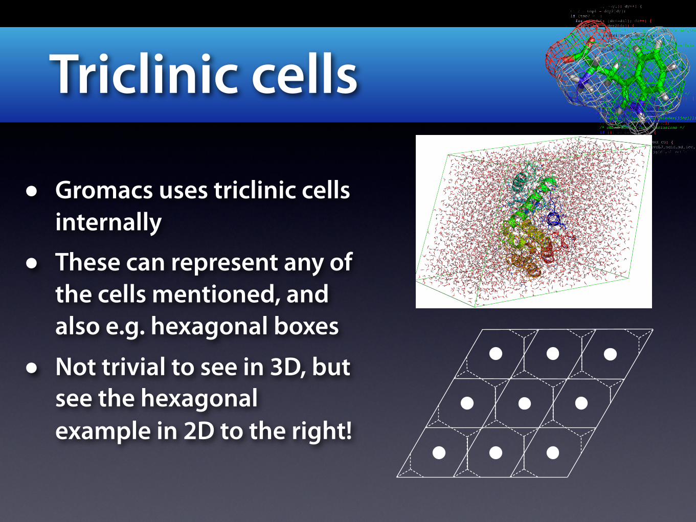
Triclinic cells

• Gromacs uses triclinic cells internally

• These can represent any of the cells mentioned, and also e.g. hexagonal boxes

• Not trivial to see in 3D, but see the hexagonal example in 2D to the right!

Lennard-Jones

• Interactions between all particles in a system

• Long range dipole dispersions: 1/r6

• Short range repulsion:Approx. 1/r12 (Really exp)

• Decays fast - cutoff fine

0.3 0.4 0.5 0.6 0.7 0.8

r (nm)

0.0

0.5

1.0

1.5

2.0

VLJ (

kJ m

ole

-1)

C12

r12i j!C6

r6i j

4!!""

r

#12!

""r

#6$

or

Electrostatics• Interactions between charged

particles

• Strong interaction - sensitive to partial charges!

• Decays very slowly; cut-offs do not even always converge!

• Charge groups can be used to guarantee convergence

14!"0

qiq j

ri j

+-

+-

Reaction-field• Assume interactions are

damped by εr beyond cut-off

• Homogeneous & isotropic

• Really cheap to calculate

• Good for dipoles, not ions

V = Vcoulomb !!

1+!r f "12!r f +1

"r3

r3cut

Ewald summation• Separate electrostatics into

long & short range parts

• Short range decays fast(cut-off can be applied)

• Long range solved in reciprocal space, just as for crystals - corresponds to sum over the infinite periodic copies!

Electrostatics – Ewald

Vsr = Vcoulomb ! er f c(r/!)Vlr = Vcoulomb ! (1" er f c(r/!))

PME• Particle-Mesh Ewald

• Modern, fast, way to perform Ewald summation

• Charge spreading on 3D grid

• Solve Poisson eq. on grid (convolution in recprocal space)

• Transform back, interpolate to get forces

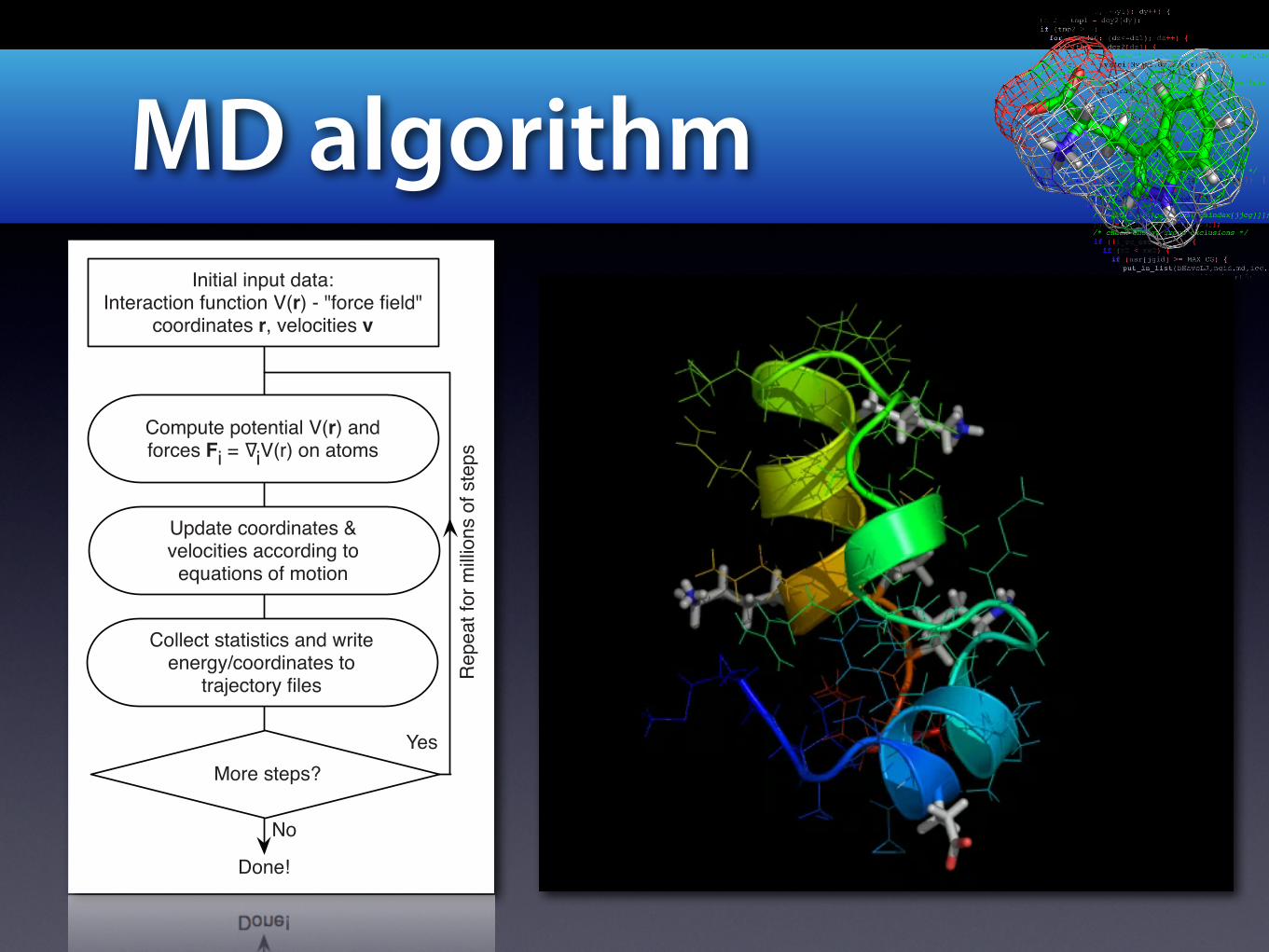
MD algorithm

Update coordinates & velocities according to equations of motion

More steps?

Compute potential V(r) andforces Fi = iV(r) on atoms

Initial input data:Interaction function V(r) - "force field"

coordinates r, velocities v

Collect statistics and write energy/coordinates to

trajectory files

Done!

Yes

No

Repe

at for

milli

ons o

f step

s

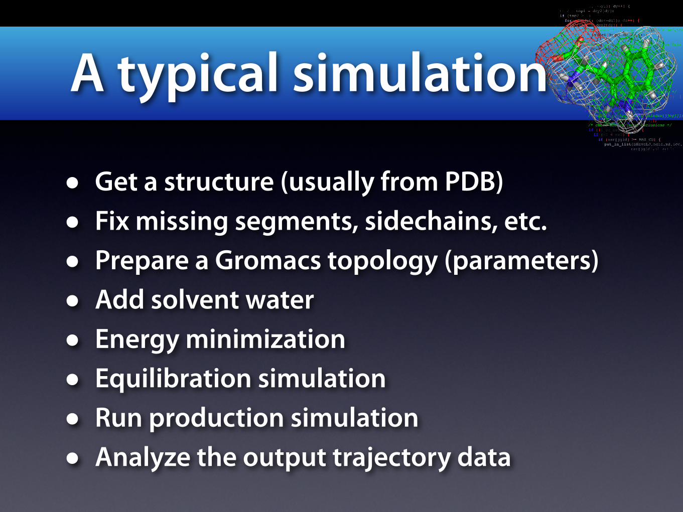
A typical simulation

• Get a structure (usually from PDB)

• Fix missing segments, sidechains, etc.

• Prepare a Gromacs topology (parameters)

• Add solvent water

• Energy minimization

• Equilibration simulation

• Run production simulation

• Analyze the output trajectory data

Energy Minimization

• Find local energy minima

• ...or rather: avoid maxima

• Forces are gradient of V

• Example algorithms:Steepest descentConjugate gradientsL-BFGS

• Normally small changes

Ensembles• How do we reproduce experimental

conditions like temperature & pressure?

• Temperature = Kinetic energySet from Maxwell distribution

• Has to be controlled during simulation, since we lose energy, e.g. due to cut-offs

• Berk will cover this in detail next hour!

• Pressure: Control by adjusting cell size

• Chemical potential: Add/remove particles

Water models

• To speed up simulation we normally use simplified models for water

• Assume water molecules to be rigid to avoid hydrogen vibrations

• Common models: SPC, TIP3P, TIP4P

• There is a wealth of advanced models when you are more interested in water properties per se (also polarization)

Limitations of MD• Parameters are imperfect

• Phase space is not sampled exhaustively

• Example: Free energies of solvation for amino acids often have errors ~1kJ/mol

• Likely impossible to calculate binding free energies more accurately than this

• Limited polarization effects; waters can reorient, but partial charges are fixed

It’s statistical mechanics!

• Remember:Just because you see something in a simulation does NOT mean it is real

• Everything is about statistics

• When you’ve seen it 10 times it’s significant - a single event is not!

• You should always try to calculate error estimates for predicted properties

MD Programs• GROMACS, Amber, Charmm, NAMD,

ESPRESSO, Encad, BOSS, LAMMPS

• Programs are often intimately tied to a force field (Amber99, Charmm19, OPLS)

• Force fields supported by Gromacs: GROMOS96, Gromacs, OPLS-AA/L, Amber, Encad, Charmm (beta), etc.

• Try to stick to 1-2 programs, and learn them in detail - you need to motivate your choice of algorithms when publishing!

A typical simulation

• Get a structure (usually from PDB)

• Fix missing segments, sidechains, determine protonation states, etc.

• Prepare a Gromacs topology (parameters)

• Add solvent water

• Energy minimization

• Equilibration simulation

• Run production simulation

• Analyze the output trajectory data

Summary

• Think first, then simulate

• Timescales & limitations

• Empirical classical models

• Interaction forms

• Sampling equilibrium distributions

• Algorithms, approximations, quality

• Flowcharts of typical simulations