Page 1
USGS Home
Contact USGS Search USGS
USGS Status and Trends of Biological Resources - NPS Inventory and Monitoring
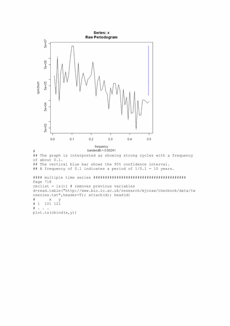
Learn R R is a free software environment for statistical computing and
graphics.
http://www.r-project.org/ Home | Getting Started | Schedule | References | FAQ | Discussion |
Tom's site | Other Courses For more information, please contact Paul Geissler
([email protected] ). Previous page
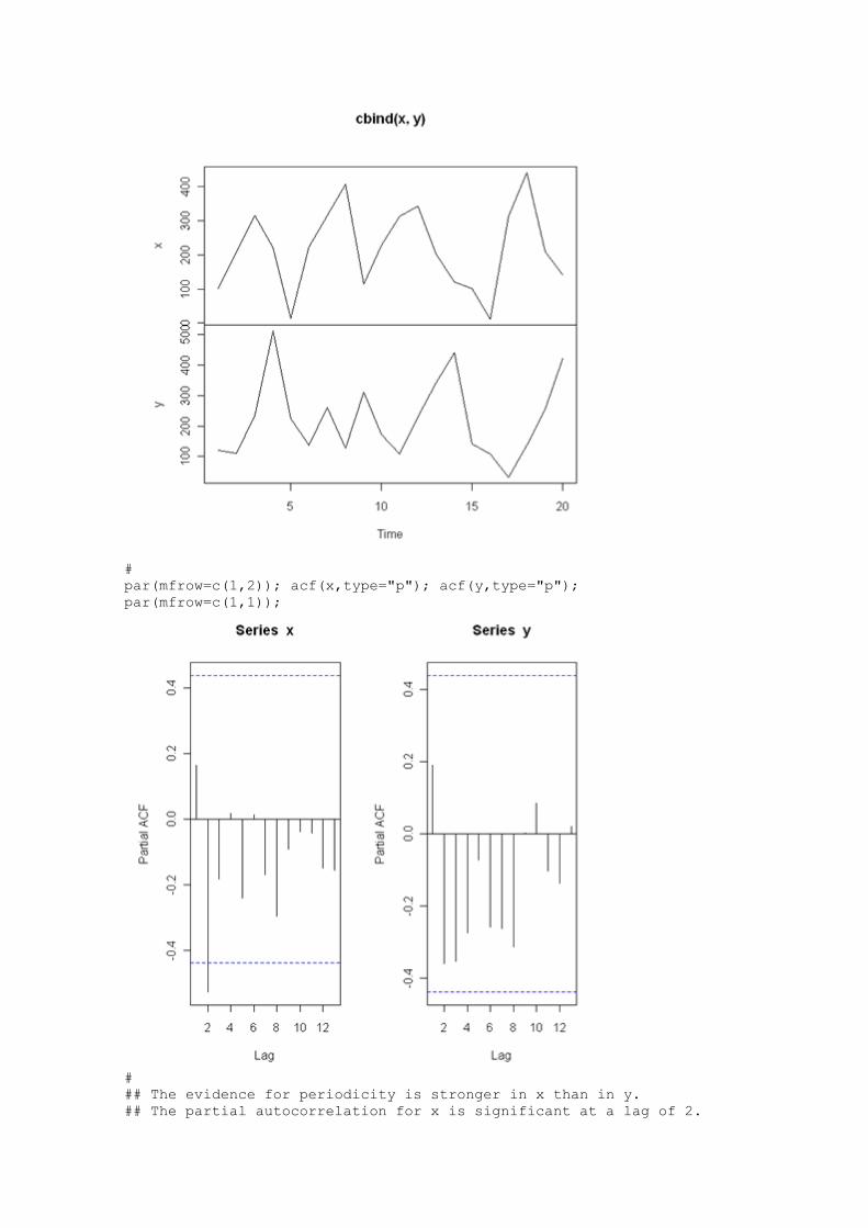
Topic 10 - Introduction to R
Graphics Contents:
graphics packages help & documentation
graphics in base package plot
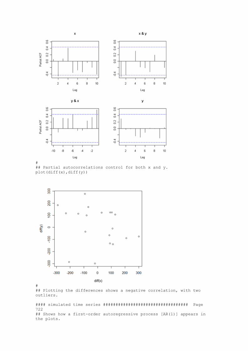
scatterplot hist
lattice graphics package univariate
bivariate: trivariate:
hypervariate:
arguments multipanel displays
panel functions gplots package
Graphic Packages There are many graphics packages available for R. We will only look
at a few of them. • agsemisc - Miscellaneous plotting and utility functions - High-
featured panel functions for bwplot and xyplot, various plot
Page 2
management helpers,
some other utility functions • aplpack - Another Plot PACKage - A set of functions for drawing
some special plots: stem.leaf plots a stem and leaf plot bagplot plots
a bagplot faces plots chernoff faces spin3R enables you an inspection of a 3-dim point cloud
• base graphics - built into R • dynamicGraph - Interactive graphical tool for manipulating graphs
- • gclus - Clustering Graphics - Orders panels in scatterplot matrices
and parallel coordinate displays by some merit index. Package contains various indices of merit, ordering functions,
and enhanced versions of pairs and parcoord which color panels according to their merit level.
• ggplot - An implementation of the Grammar of Graphics in R - An implementation of the grammar of graphics in R. It combines the
advantages of both base and lattice graphics: conditioning and shared axes are handled automatically, and you can still build up a
plot step by step from multiple data sources. It also implements a
more sophisticated multidimensional conditioning system and a consistent interface to map data to aesthetic attributes. See
http://had.co.nz/ggplot/ for more information, documentation and examples.
• gplots - Various R programming tools for plotting data • gridBase - Integration of base and grid graphics
• iplots - interactive graphics for R - Interactive plots for R • lattice - Implementation of Trellis Graphics.
• latticeExtra - Extra Graphical Displays based on lattice - Generic function and standard methods for Trellis-based displays
• misc3d - Miscellaneous 3D Plots - A collection of miscellaneous 3d plots, including isos
Help & Documentation Reference Manuals: To view the reference manuals for packages go
to CRAN (Comprehansive R Archive Network, http://www.r-project.org/ ) and pick a mirror site (e.g.,
http://lib.stat.cmu.edu/R/CRAN/), select "Packages" on the left and then select the package you are interested in. The reference manual
will be available as a PDF file. These manual are more complete than the help files. Consider the R Reference Card.
Help Files: From the R Commander script window or the R console
enter the command ?lattice for example for the lattice package. The help files are very useful but somewhat terse. They are intended
more for reference than for learning about a package or command. Search: To search for help, go to the CRAN site (http://www.r-
project.org/ ) and click on "Search" on the left. Notation: I will use italics to indicate S commands to be submitted
to R.
Page 3
References:
• J H Maindonald, 2008, Using R for Data Analysis and Graphics, http://cran.r-project.org/doc/contrib/usingR.pdf
• Nicholas Lewin-Koh, 2010, CRAN Task View: Graphic Displays &
Dynamic Graphics & Graphic Devices & Visualization, http://cran.r-project.org/web/views/Graphics.html
• M.J. Crawley, 2007. The R Book, Wiley, Chapter 5 • Paul Murrell, 2006. R Graphics, Chapman & Hall. This is an essential
reference to customize graphics.
graphics in base package References: • An Introduction to R: Software for Statistical Modeling & Computing
by Petra Kuhnert and Bill Venables ( http://cran.r-project.org/doc/contrib/Kuhnert+Venables-R_Course_Notes.zip )
Free. Good introduction. • Michael J. Crawley 2007 (The R Book, Wiley) Chapter 5.
• Paul Murrell, 2006 ( R Graphics) Chapman & Hall • John Fox 2002. (An R and S-Plus companion to applied Regression.
Sage Publications, http://socserv.mcmaster.ca/jfox/Books/Companion/index.html)
provides an excellent introduction to the graphics in the base package, as well as writing commands and scripts.
The R file for this topic is available at ftp://ftpext.usgs.gov/pub/cr/co/fort.collins/Geissler/LearnR/LearnR10
-11.R . You can copy and paste this link into the Tinn-R open file
command. plot
Help is available by submitting the command ?plot (i.e., entering it in the R Commander script window, highlighting it and clicking submit).
Click on "par" to see a listing of the parameters. Some common parameters are:
x vector with x coordinates
y vector with x coordinates
type
"p" for points,
"l" for lines, "b" for both,
"c" for the lines part alone of "b" , "o" for both 'overplotted',
"h" for histogram like (or 'high-density') vertical lines, "s" for stair steps,
"S" for other steps, see Details below, "n" for no plotting.
main main title on top
sub sub title on bottom
xlab x axis label
Page 4
ylab y axis label
asp aspect ratio
xlim limits on x axis, e.g., c(0,15)
ylim limits on y axis, e.g., c(0,15)
log logarithmic axes: 'x', 'y', or 'xy'
axes=F suspresses drawing of axes and the box
cex character expansion specifies the size of points, default is 1
mex margin expansion specifies the size of the margins
col color
lty line type (0=blank, 1=solid, 2=dashed, 3=dotted,
4=dotdash, 5=longdash, 6=twodash)
lwd line width, default 1
Examples: Submit from R Commander script window.
?plot data(austpop, package="DAAG")
attach(austpop) ?austpop
# default plot(year,ACT) # vector of x values, vector of y values, can also be
written in model form as plot(y ~ x) plot(ACT~year)
Page 5
# you can idtintify point with the curser. Press Escape when you are
finished. #!!!! submit the following line from the R Console because identify()
locks up R Commander # To recover, press alt-ctrl-delete and select the task manager. Then
end R. plot(ACT~year); identify(ACT~year)
Page 6
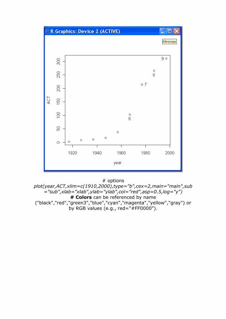
# options plot(year,ACT,xlim=c(1910,2000),type="b",cex=2,main="main",sub
="sub",xlab="xlab",ylab="ylab",col="red",asp=0.5,log="y") # Colors can be referenced by name
("black","red","green3","blue","cyan","magenta","yellow","gray") or by RGB values (e.g., red="#FF0000").
Page 7
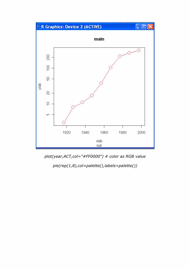
plot(year,ACT,col="#FF0000") # color as RGB value
pie(rep(1,8),col=palette(),labels=palette())
Page 8
pie(rep(1,50),col=rainbow(50))
pie(rep(1,50),col=gray(0:50/50))
Page 9
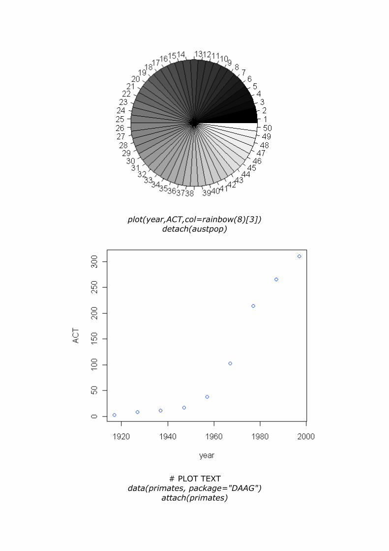
plot(year,ACT,col=rainbow(8)[3]) detach(austpop)
# PLOT TEXT data(primates, package="DAAG")
attach(primates)
Page 10
plot(Bodywt, Brainwt,xlim=c(0,300),xlab="Body weight
(kg)",ylab="Brain weight (g)",main="Brian Weight Versus Body Weight")
# highlight the main line and all the indented lines and submit them
together # xlim provides more space on right for labels
text(x=Bodywt, y=Brainwt, labels=row.names(primates), pos=4) # submit together with the plot statement
# pos= 1=below, 2=left, 3=above and 4=right detach(primates)
# ADD POINTS & LINES TO A PLOT
plot(1:25,xlab="Symbol Number",ylab="",type="n") for (pch in 1:25) points(pch,pch,pch=pch) # submit with the above
line lines(1:25, type="h",lty=2) # submit with the above line
lines(1:25, type="h",lty="dotted") # alternate to above line
Page 11
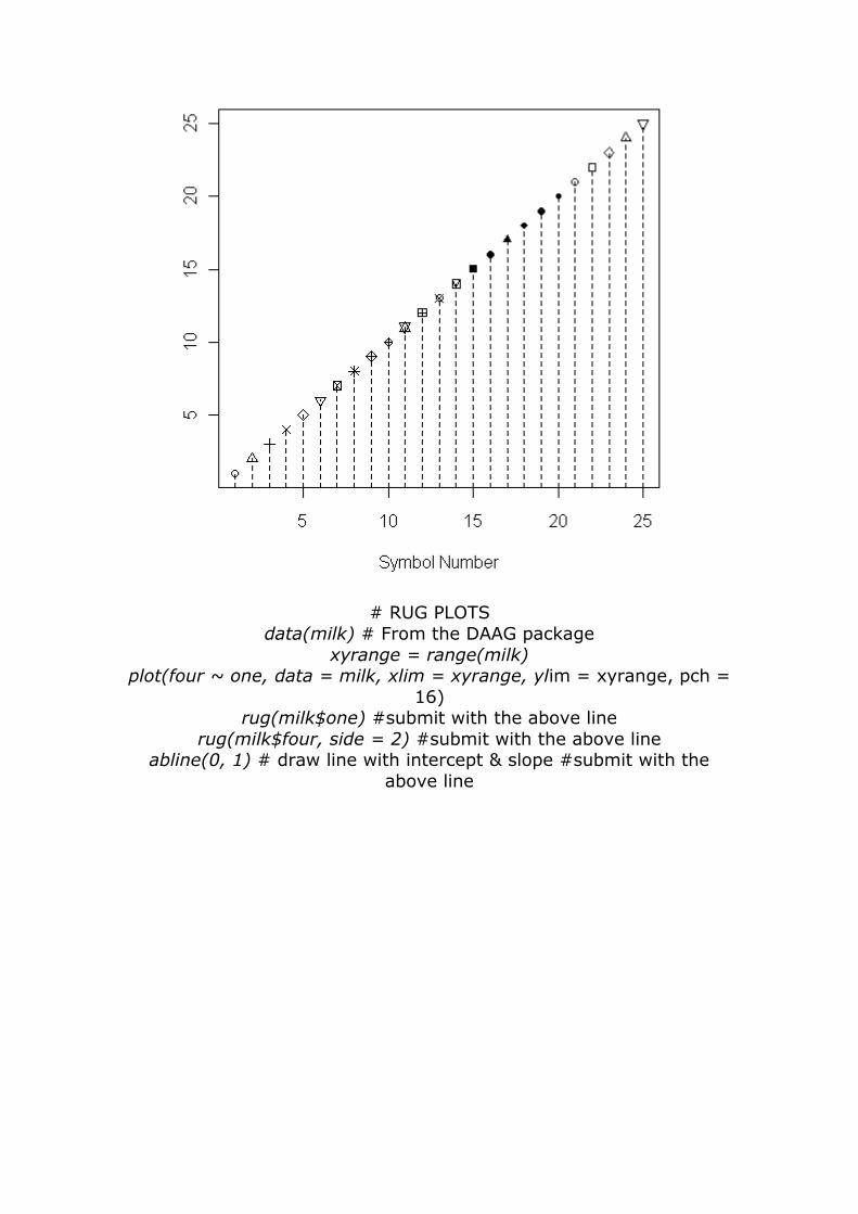
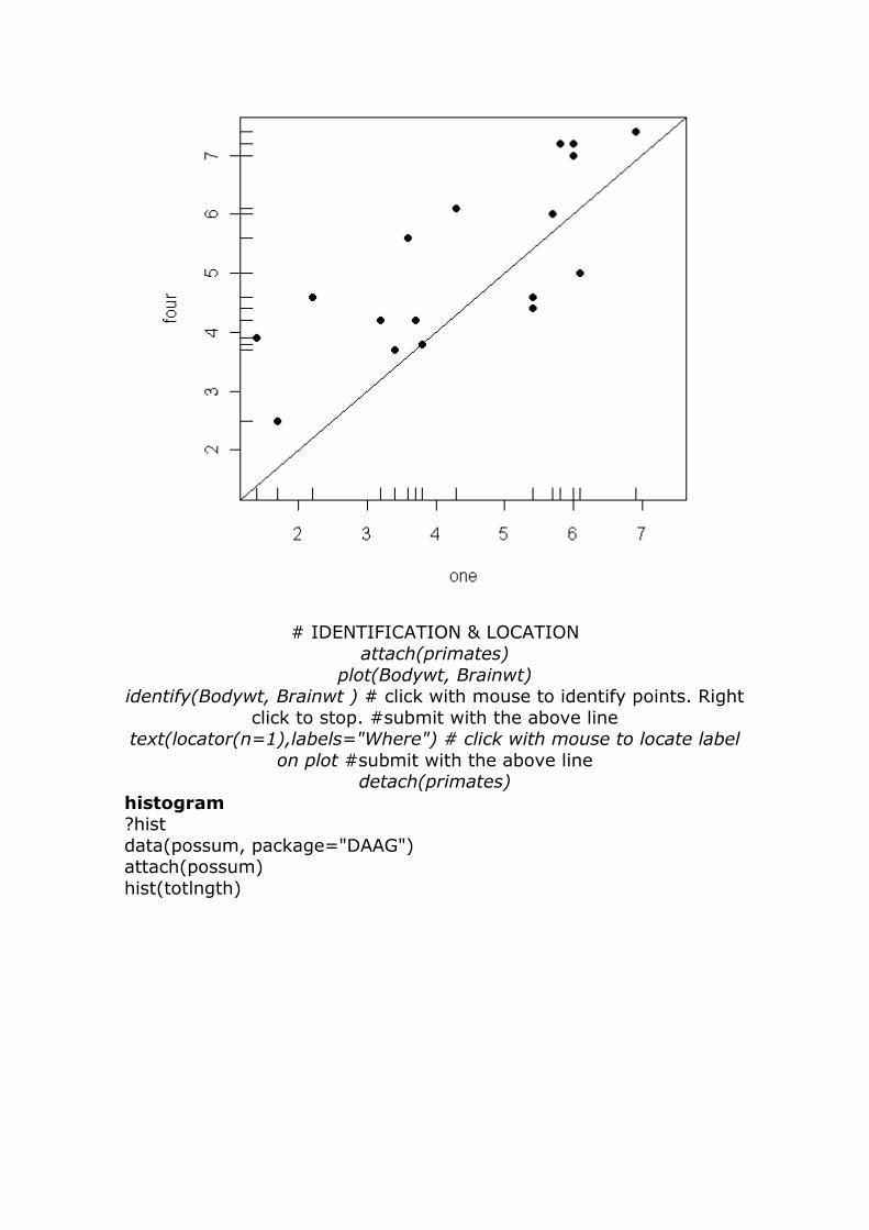
# RUG PLOTS
data(milk) # From the DAAG package
xyrange = range(milk) plot(four ~ one, data = milk, xlim = xyrange, ylim = xyrange, pch =
16) rug(milk$one) #submit with the above line
rug(milk$four, side = 2) #submit with the above line abline(0, 1) # draw line with intercept & slope #submit with the
above line
Page 12
# IDENTIFICATION & LOCATION
attach(primates)
plot(Bodywt, Brainwt) identify(Bodywt, Brainwt ) # click with mouse to identify points. Right
click to stop. #submit with the above line text(locator(n=1),labels="Where") # click with mouse to locate label
on plot #submit with the above line detach(primates)
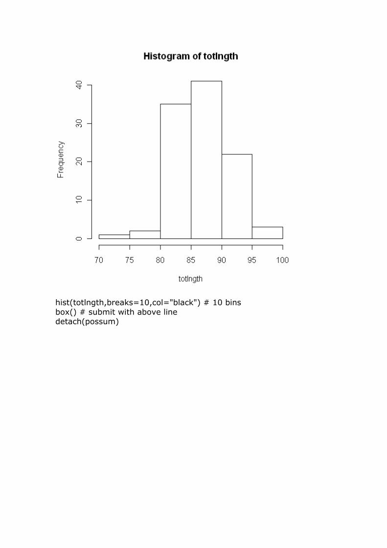
histogram ?hist
data(possum, package="DAAG") attach(possum)
hist(totlngth)
Page 13
par(mfrow=c(1,2)) # plots more than one graph in 1 row and 2 columns
hist(totlngth) hist(totlngth,breaks=seq(70,100,5)) # breaks at 70, 75, 80, ..., 100
par(mfrow=c(1,1)) # resets
Page 14
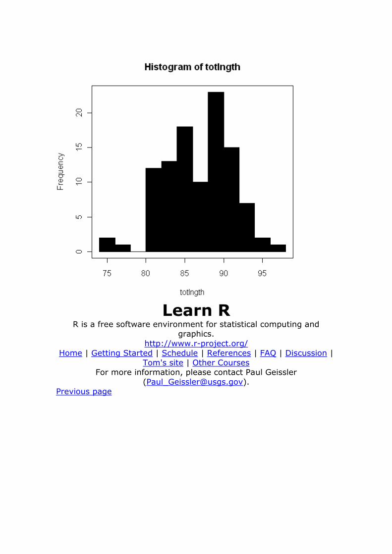
hist(totlngth,breaks=10,col="black") # 10 bins
box() # submit with above line detach(possum)
Page 15
Learn R R is a free software environment for statistical computing and
graphics.
http://www.r-project.org/ Home | Getting Started | Schedule | References | FAQ | Discussion |
Tom's site | Other Courses For more information, please contact Paul Geissler
([email protected] ). Previous page
Page 16
Topic 11 - Introduction to R Graphics - continued Other Packages Each of these packages must be installed before being used for the first time. Then before each use submit a library command.
library(lattice) library(gplots)
library(car) # Companion to Applied Regression
library(sciplot) lattice Graphics Package
Lattice in the open source version of the S-Plus Trellis Graphics Package. Lattice has functions that parallel the functions in the base
graphics package, but lattice has many more options and can place the plots in a multi-panel display, like a lattice or trellis.
Documentation: • Becker, R. A. and W. S. Cleveland. 1996. S-Plus Trellis Graphics
User's Manual http://cm.bell-labs.com/stat/doc/trellis.user.pdf • Sarkar, D. Lattice user's manual
http://lib.stat.cmu.edu/R/CRAN/web/packages/lattice/lattice.pdf • Enter command ?lattice for help
This presentation will follow Becker and Cleveland (1996). The high level plotting functions are:
Univariate:
barchart - bar plots bwplot - box and whisker plots
densityplot - kernel density plots dotplot - dot plots
histogram - histograms qqmath - quantile plots against mathematical distributions
stripplot - 1-dimensional scatterplot Bivariate:
qq - quantile-quantile plot for comparing two distributions xyplot - scatter plot (and possibly a lot more)
Trivariate: levelplot - level plots (similar to image plots in R)
contourplot - contour plots cloud - 3-D scatter plots
wireframe - 3-D surfaces (similar to persp plots in R)
Hypervariate: splom - scatterplot matrix
parallel - parallel coordinate plots Miscellaneous:
rfs - residual and fitted value plot (also see oneway) tmd - Tukey Mean-Difference plot
Page 17
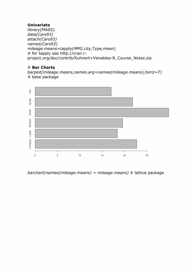
Univariate
library(MASS) data(Cars93)
attach(Cars93)
names(Cars93) mileage.means=tapply(MPG.city,Type,mean)
# for tapply see http://cran.r-project.org/doc/contrib/Kuhnert+Venables-R_Course_Notes.zip
# Bar Charts
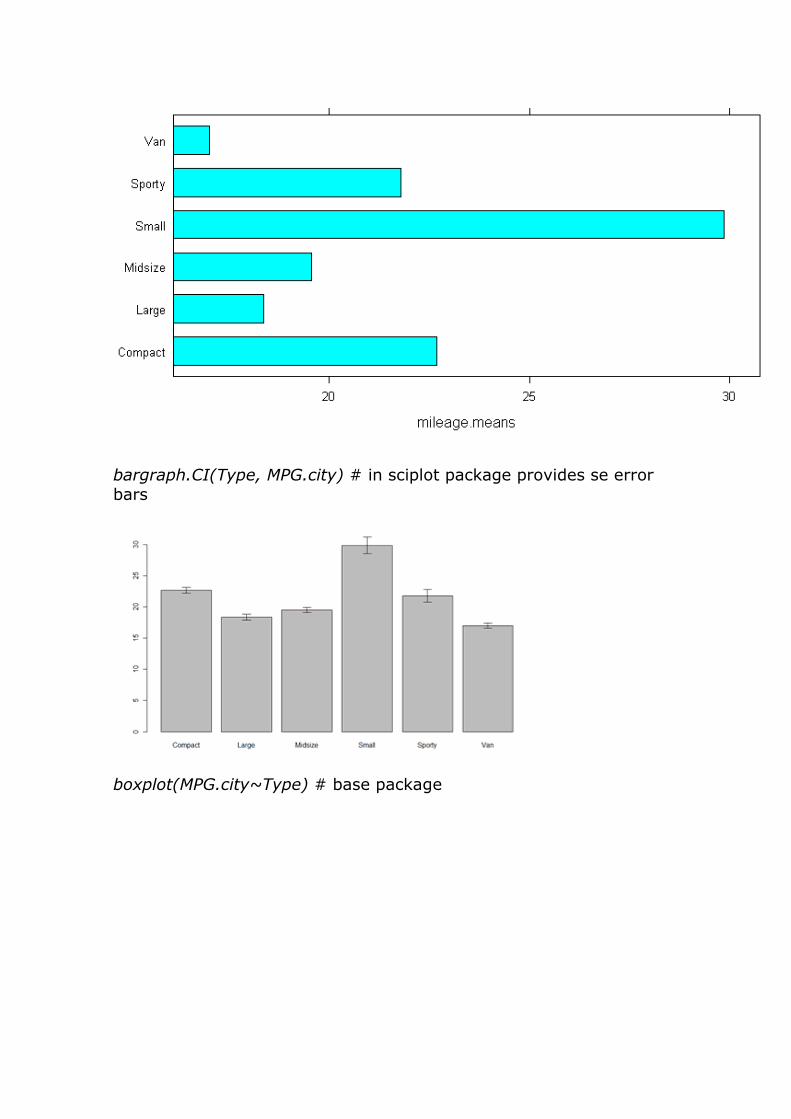
barplot(mileage.means,names.arg=names(mileage.means),horiz=T) # base package
barchart(names(mileage.means) ~ mileage.means) # lattice package
Page 18
bargraph.CI(Type, MPG.city) # in sciplot package provides se error
bars
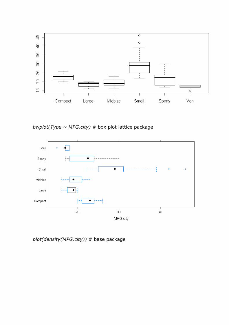
boxplot(MPG.city~Type) # base package
Page 19
bwplot(Type ~ MPG.city) # box plot lattice package
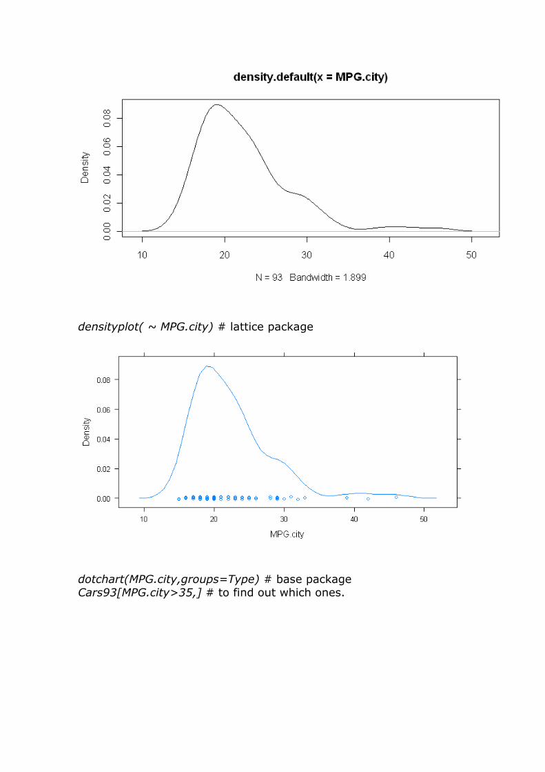
plot(density(MPG.city)) # base package
Page 20
densityplot( ~ MPG.city) # lattice package
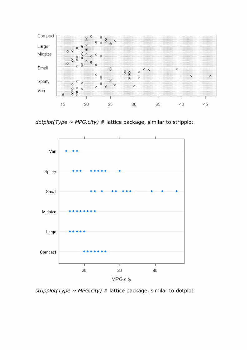
dotchart(MPG.city,groups=Type) # base package Cars93[MPG.city>35,] # to find out which ones.
Page 21
dotplot(Type ~ MPG.city) # lattice package, similar to stripplot
stripplot(Type ~ MPG.city) # lattice package, similar to dotplot
Page 22
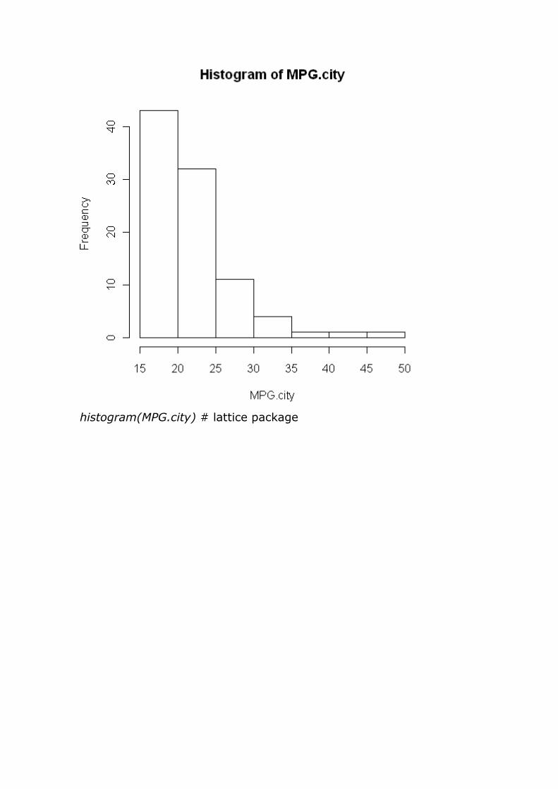
hist(MPG.city) # base package
Page 23
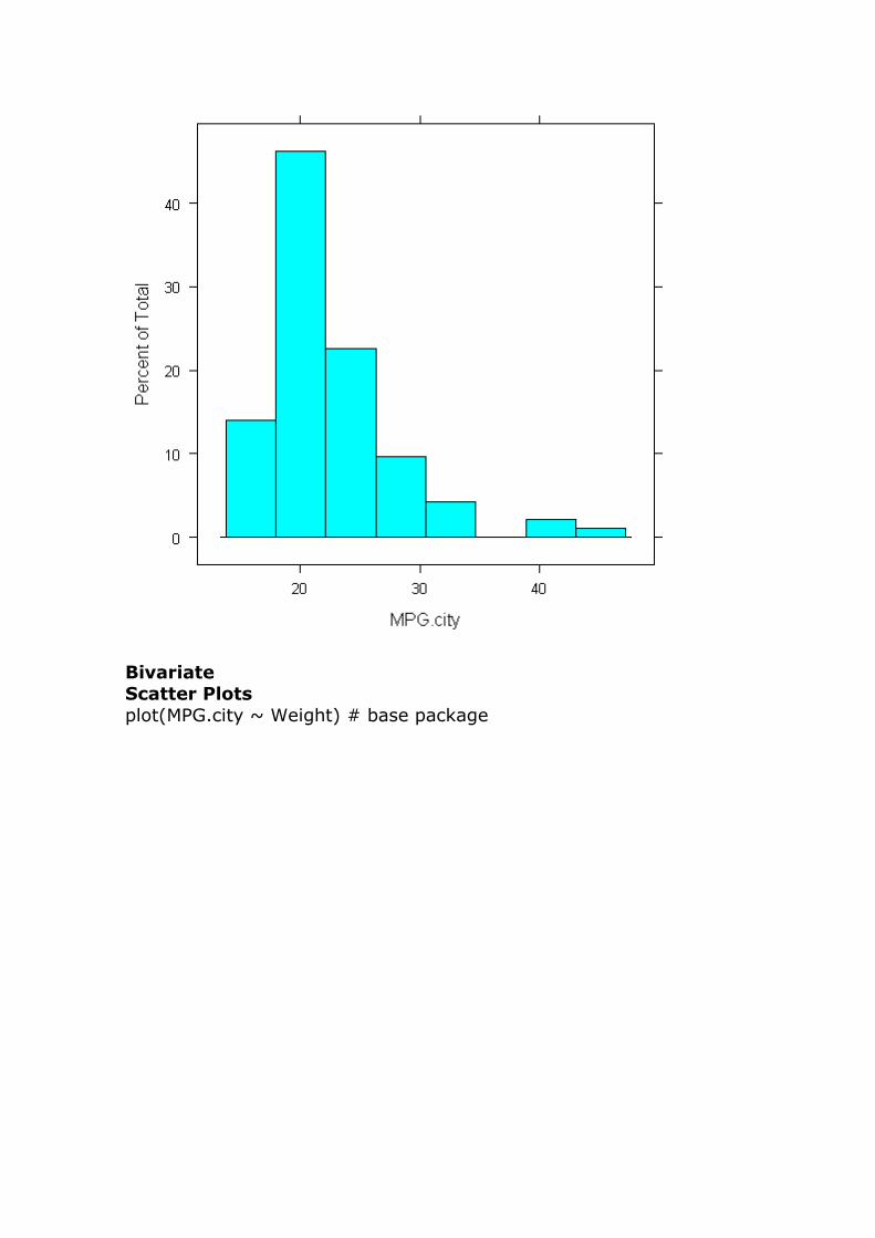
histogram(MPG.city) # lattice package
Page 24
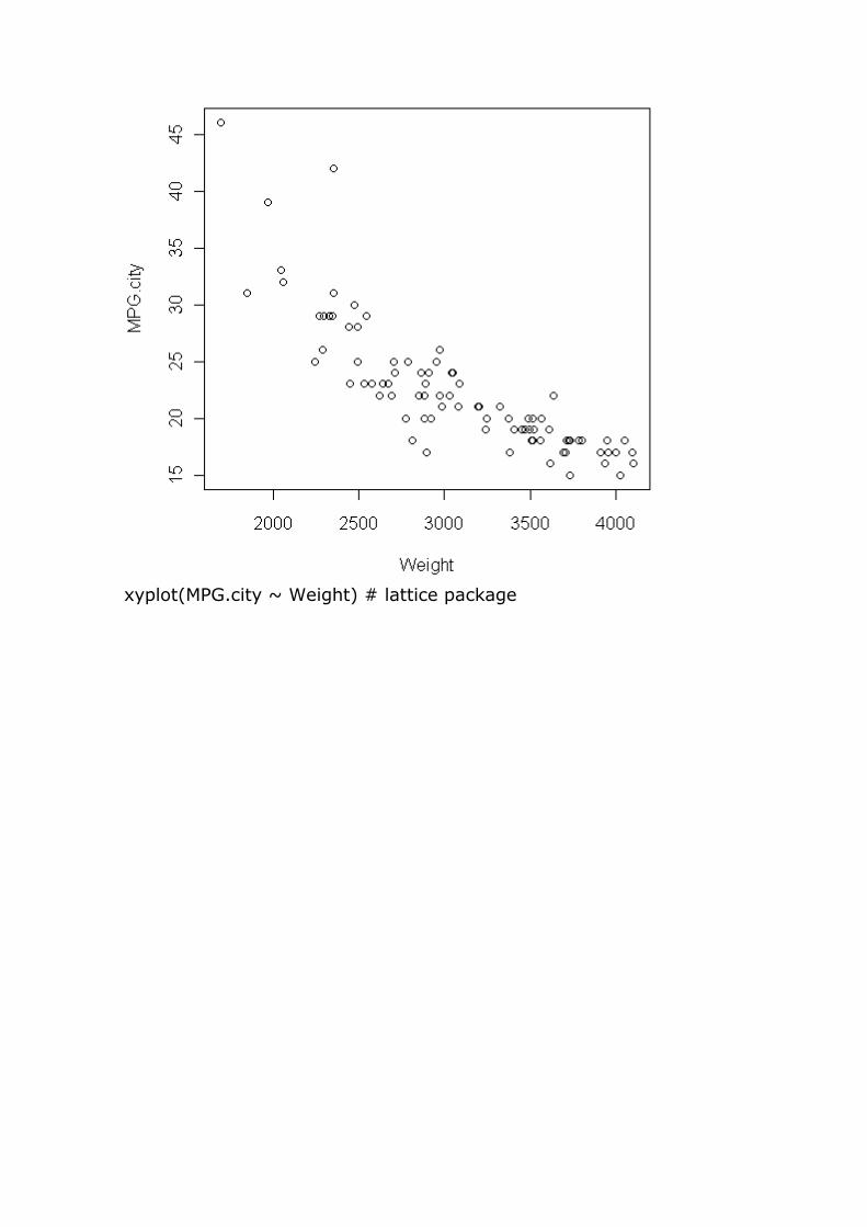
Bivariate Scatter Plots
plot(MPG.city ~ Weight) # base package
Page 25
xyplot(MPG.city ~ Weight) # lattice package
Page 26
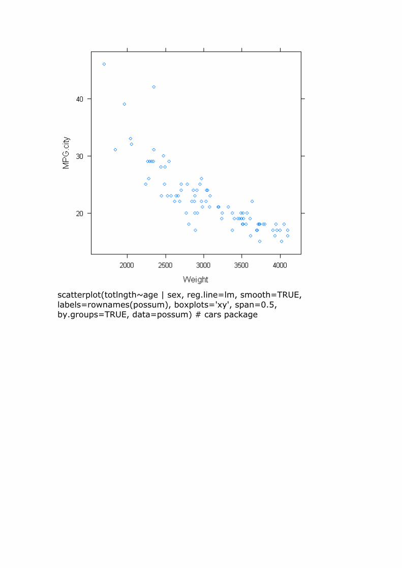
scatterplot(totlngth~age | sex, reg.line=lm, smooth=TRUE,
labels=rownames(possum), boxplots='xy', span=0.5, by.groups=TRUE, data=possum) # cars package
Page 27
Quantile-Quantile Plots
qq.plot(MPG.city, distribution="norm") # base package
Page 28
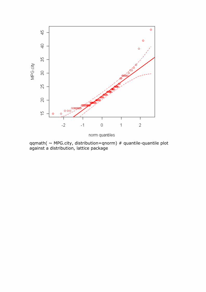
qqmath( ~ MPG.city, distribution=qnorm) # quantile-quantile plot
against a distribution, lattice package
Page 29
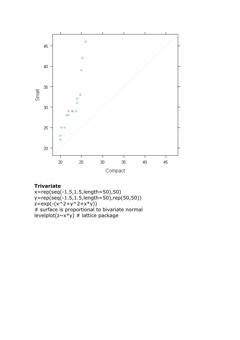
qq(Type ~ MPG.city,subset=(Type=="Compact" | Type=="Small")) #
quantile-quantile plot for 2 data sets - lattice package detach(Cars93)
Page 30
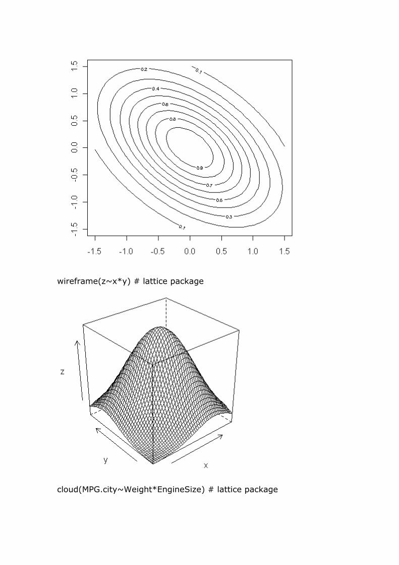
Trivariate x=rep(seq(-1.5,1.5,length=50),50)
y=rep(seq(-1.5,1.5,length=50),rep(50,50)) z=exp(-(x^2+y^2+x*y))
# surface is proportional to bivariate normal levelplot(z~x*y) # lattice package
Page 31
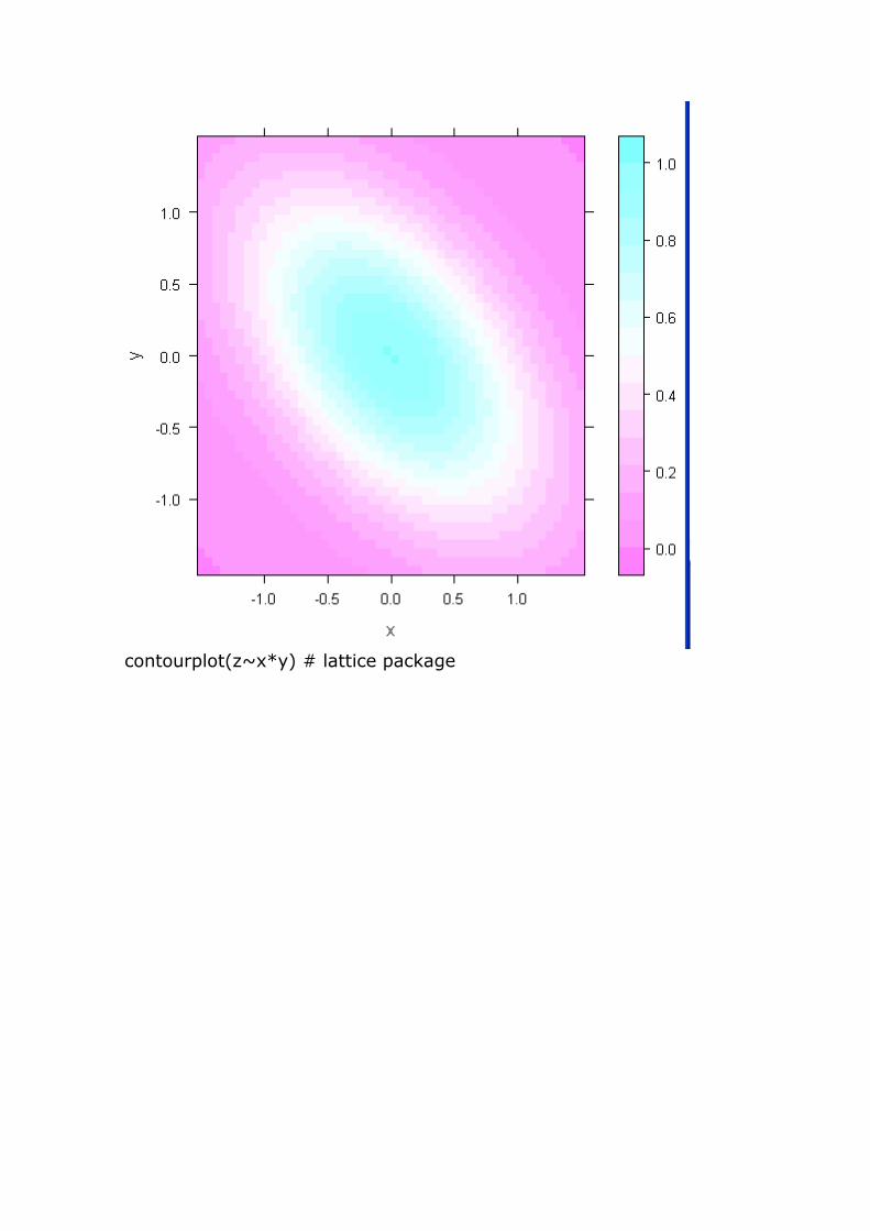
contourplot(z~x*y) # lattice package
Page 32
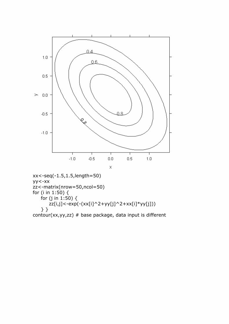
xx<-seq(-1.5,1.5,length=50) yy<-xx
zz<-matrix(nrow=50,ncol=50) for (i in 1:50) {
for (j in 1:50) { zz[i,j]<-exp(-(xx[i]^2+yy[j]^2+xx[i]*yy[j]))
} } contour(xx,yy,zz) # base package, data input is different
Page 33
wireframe(z~x*y) # lattice package
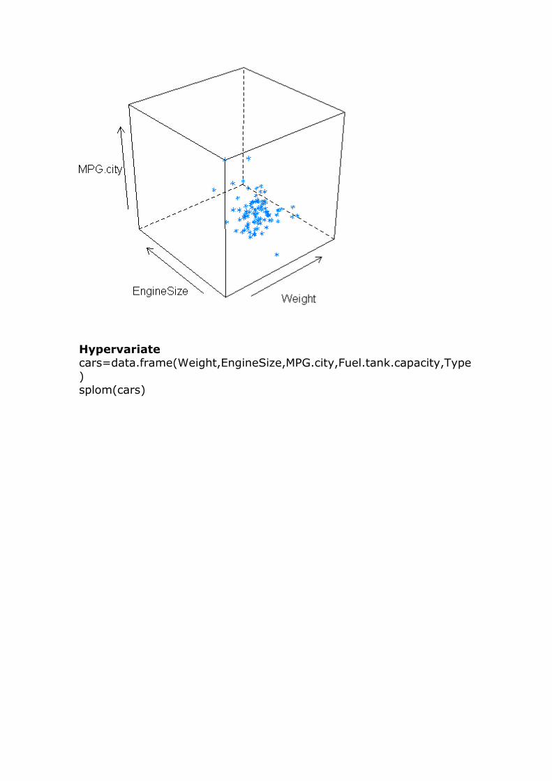
cloud(MPG.city~Weight*EngineSize) # lattice package
Page 34
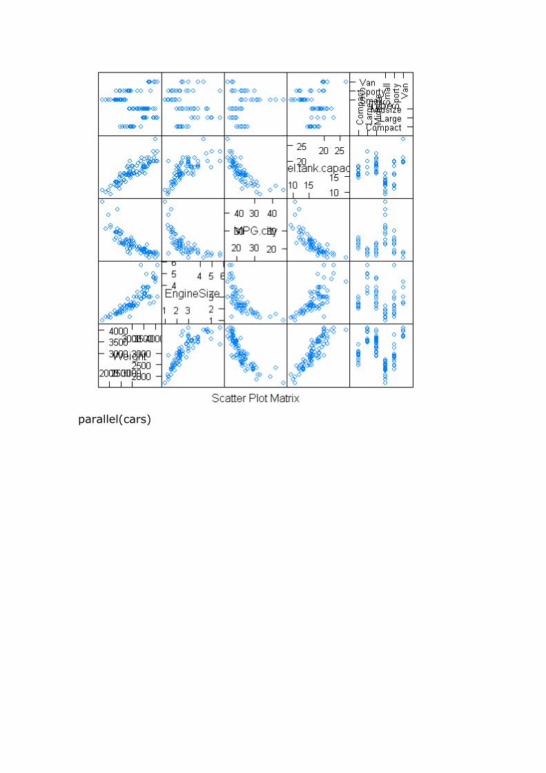
Hypervariate cars=data.frame(Weight,EngineSize,MPG.city,Fuel.tank.capacity,Type
) splom(cars)
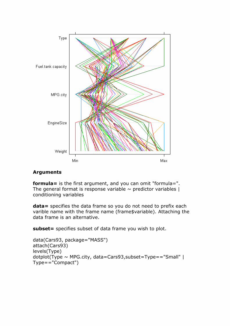
Page 36
Arguments
formula= is the first argument, and you can omit "formula=". The general format is response variable ~ predictor variables |
conditioning variables
data= specifies the data frame so you do not need to prefix each varible name with the frame name (frame$variable). Attaching the
data frame is an alternative.
subset= specifies subset of data frame you wish to plot.
data(Cars93, package="MASS")
attach(Cars93) levels(Type)
dotplot(Type ~ MPG.city, data=Cars93,subset=Type=="Small" | Type=="Compact")
Page 37
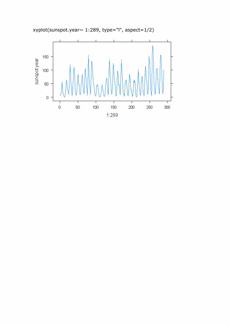
aspect= aspect ratio. "xy" sets the aspect ratio to bank to 45° which is often optimal.
data(sunspot.year, package="datasets")
xyplot(sunspot.year~ 1:289, type="l") # from 1849 to 1924
Page 38
xyplot(sunspot.year~ 1:289, type="l", aspect="xy") # shows that sunspots rise more rapidly than they fall
Page 39
xyplot(sunspot.year~ 1:289, type="l", aspect=1/2)
Page 40
Topic 11 - Introduction to R Graphics - continued
Displays
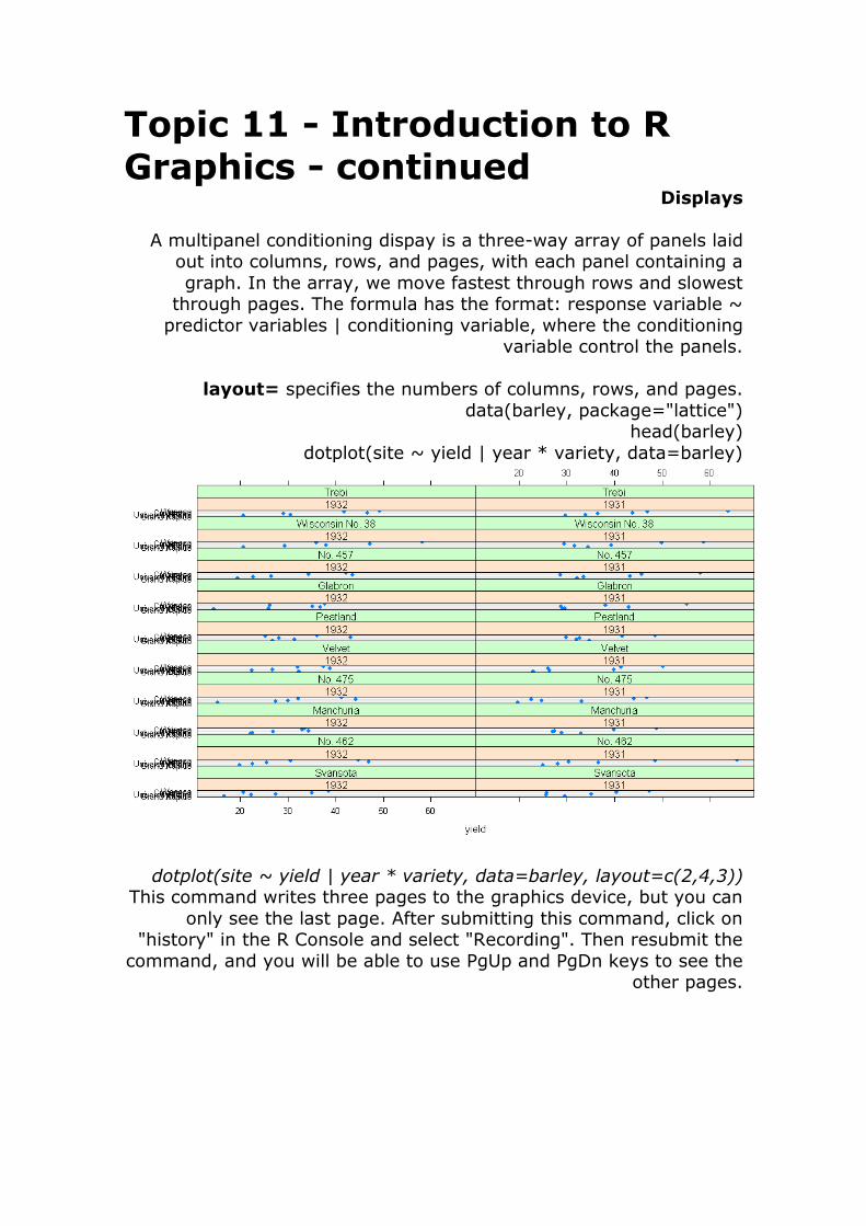
A multipanel conditioning dispay is a three-way array of panels laid out into columns, rows, and pages, with each panel containing a
graph. In the array, we move fastest through rows and slowest through pages. The formula has the format: response variable ~
predictor variables | conditioning variable, where the conditioning variable control the panels.
layout= specifies the numbers of columns, rows, and pages.
data(barley, package="lattice") head(barley)
dotplot(site ~ yield | year * variety, data=barley)
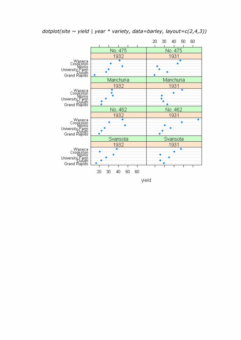
dotplot(site ~ yield | year * variety, data=barley, layout=c(2,4,3)) This command writes three pages to the graphics device, but you can
only see the last page. After submitting this command, click on "history" in the R Console and select "Recording". Then resubmit the
command, and you will be able to use PgUp and PgDn keys to see the other pages.
Page 42
reorder(factor,data,function) changes the order of a conditioning
factor to facilitate perceptions.
factor = factor to be reordered data = data upon which the reordering is to be based
function = function applied to the data to provide the reordering. barley$variety = reorder(barley$variety,barley$yield, median)
Page 43
dotplot(site ~ yield | year * variety, data=barley, layout=c(2,4,3))
Page 44
equal.count() is used to condition on intervals of a numeric variable. Conditioning on a numeric varible normally uses each
unique value, but with a continuous variable there may be too many
unique values for a useful plot. The equal.count() and shingle() functions can be used to define subsets of numeric conditioning
variables for plotting. equal. The resul is an object of the class shingle, so named because the bins overlap like shingles on a roof.
Page 45
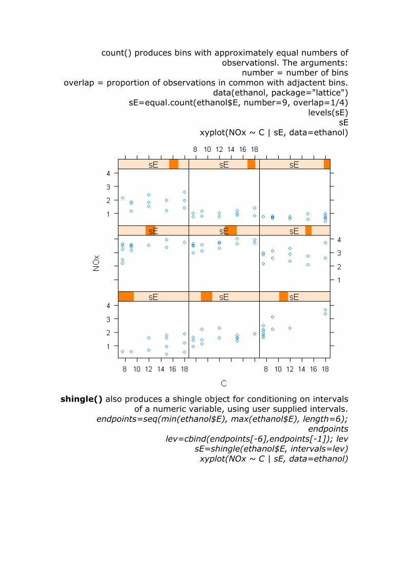
count() produces bins with approximately equal numbers of
observationsl. The arguments: number = number of bins
overlap = proportion of observations in common with adjactent bins.
data(ethanol, package="lattice") sE=equal.count(ethanol$E, number=9, overlap=1/4)
levels(sE) sE
xyplot(NOx ~ C | sE, data=ethanol)
shingle() also produces a shingle object for conditioning on intervals
of a numeric variable, using user supplied intervals.
endpoints=seq(min(ethanol$E), max(ethanol$E), length=6); endpoints
lev=cbind(endpoints[-6],endpoints[-1]); lev sE=shingle(ethanol$E, intervals=lev)
xyplot(NOx ~ C | sE, data=ethanol)
Page 46
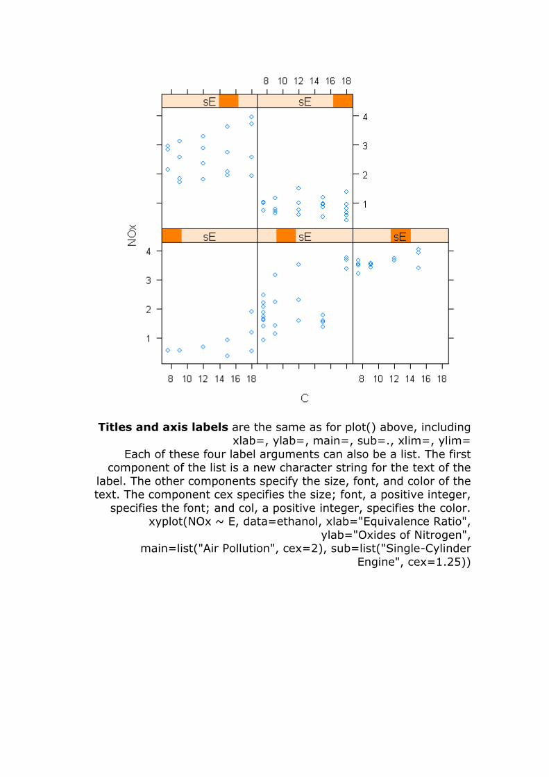
Titles and axis labels are the same as for plot() above, including
xlab=, ylab=, main=, sub=., xlim=, ylim=
Each of these four label arguments can also be a list. The first component of the list is a new character string for the text of the
label. The other components specify the size, font, and color of the text. The component cex specifies the size; font, a positive integer,
specifies the font; and col, a positive integer, specifies the color. xyplot(NOx ~ E, data=ethanol, xlab="Equivalence Ratio",
ylab="Oxides of Nitrogen", main=list("Air Pollution", cex=2), sub=list("Single-Cylinder
Engine", cex=1.25))
Page 47
scales= controls the axis lables and tick marks. xyplot(NOx ~ E, data=ethanol, scales = list(cex = 2,x =
list(tick.number = 4),y = list(tick.number = 10)))
Page 48
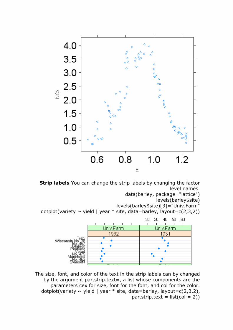
Strip labels You can change the strip labels by changing the factor level names.
data(barley, package="lattice") levels(barley$site)
levels(barley$site)[3]="Univ.Farm" dotplot(variety ~ yield | year * site, data=barley, layout=c(2,3,2))
The size, font, and color of the text in the strip labels can by changed by the argument par.strip.text=, a list whose components are the
parameters cex for size, font for the font, and col for the color. dotplot(variety ~ yield | year * site, data=barley, layout=c(2,3,2),
par.strip.text = list(col = 2))
Page 49
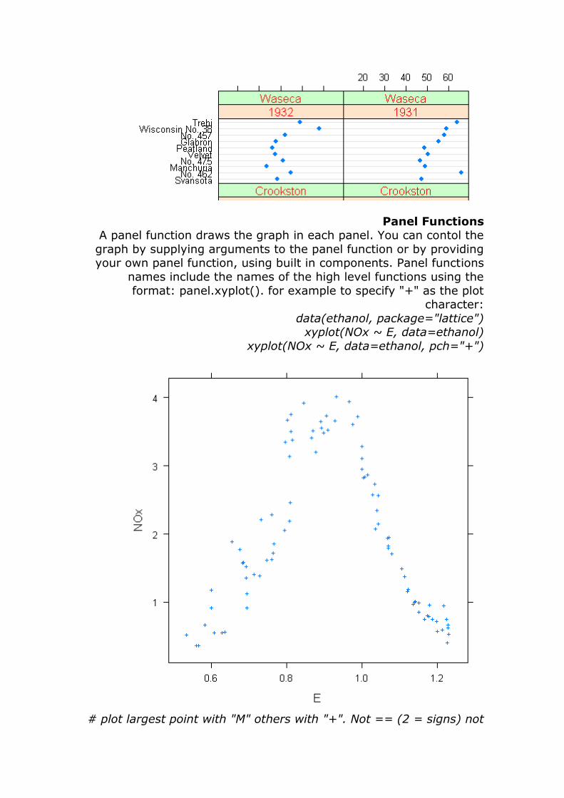
Panel Functions A panel function draws the graph in each panel. You can contol the
graph by supplying arguments to the panel function or by providing your own panel function, using built in components. Panel functions
names include the names of the high level functions using the
format: panel.xyplot(). for example to specify "+" as the plot character:
data(ethanol, package="lattice") xyplot(NOx ~ E, data=ethanol)
xyplot(NOx ~ E, data=ethanol, pch="+")
# plot largest point with "M" others with "+". Not == (2 = signs) not
Page 50
= is equality operator.
newPanel=function(x,y) { largest=y==max(y);
panel.points(x[!largest],y[!largest],pch="+");
panel.points(x[largest],y[largest],pch="M"); }
xyplot(NOx ~ E, data=ethanol, panel=newPanel)
# To overlay a smooth curvey on the plots, combine two panel
functions.
sE=equal.count(ethanol$E, number=9, overlap=1/4) newPanel=function(x,y) {
panel.xyplot(x,y);
panel.loess(x,y); } xyplot(NOx ~ C | sE, data=ethanol, panel=newPanel)
Page 51
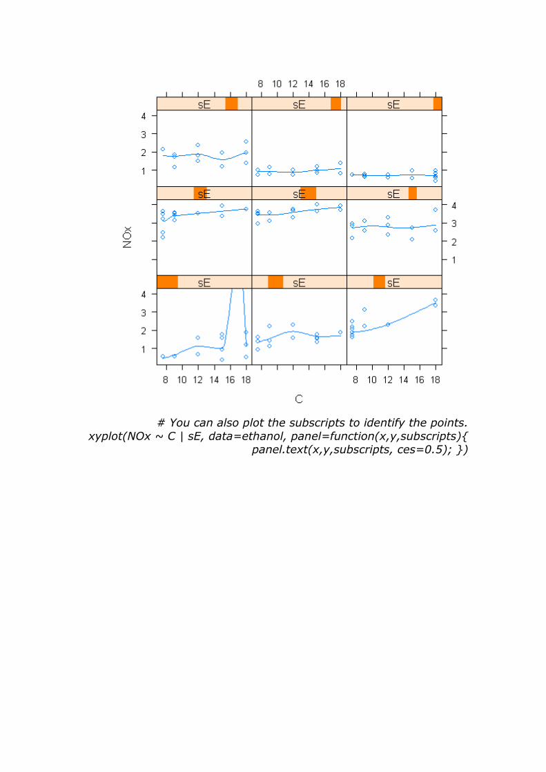
# You can also plot the subscripts to identify the points.
xyplot(NOx ~ C | sE, data=ethanol, panel=function(x,y,subscripts){ panel.text(x,y,subscripts, ces=0.5); })
Page 52
Superposition of graph elements, such as using different symbols for groups.
data(Cars93, package="MASS") attach(Cars93)
xyplot(MPG.city ~ Weight, data=Cars93, groups=Type, auto.key=T)
Page 53
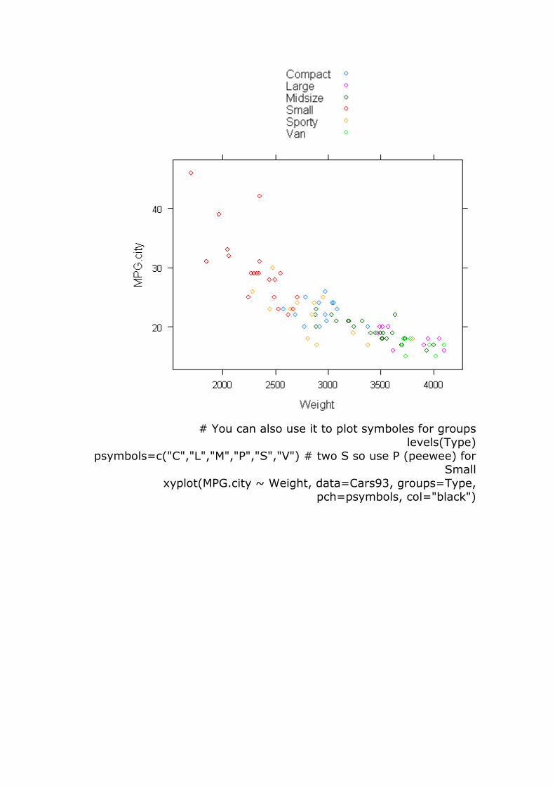
# You can also use it to plot symboles for groups
levels(Type)
psymbols=c("C","L","M","P","S","V") # two S so use P (peewee) for Small
xyplot(MPG.city ~ Weight, data=Cars93, groups=Type, pch=psymbols, col="black")
Page 54
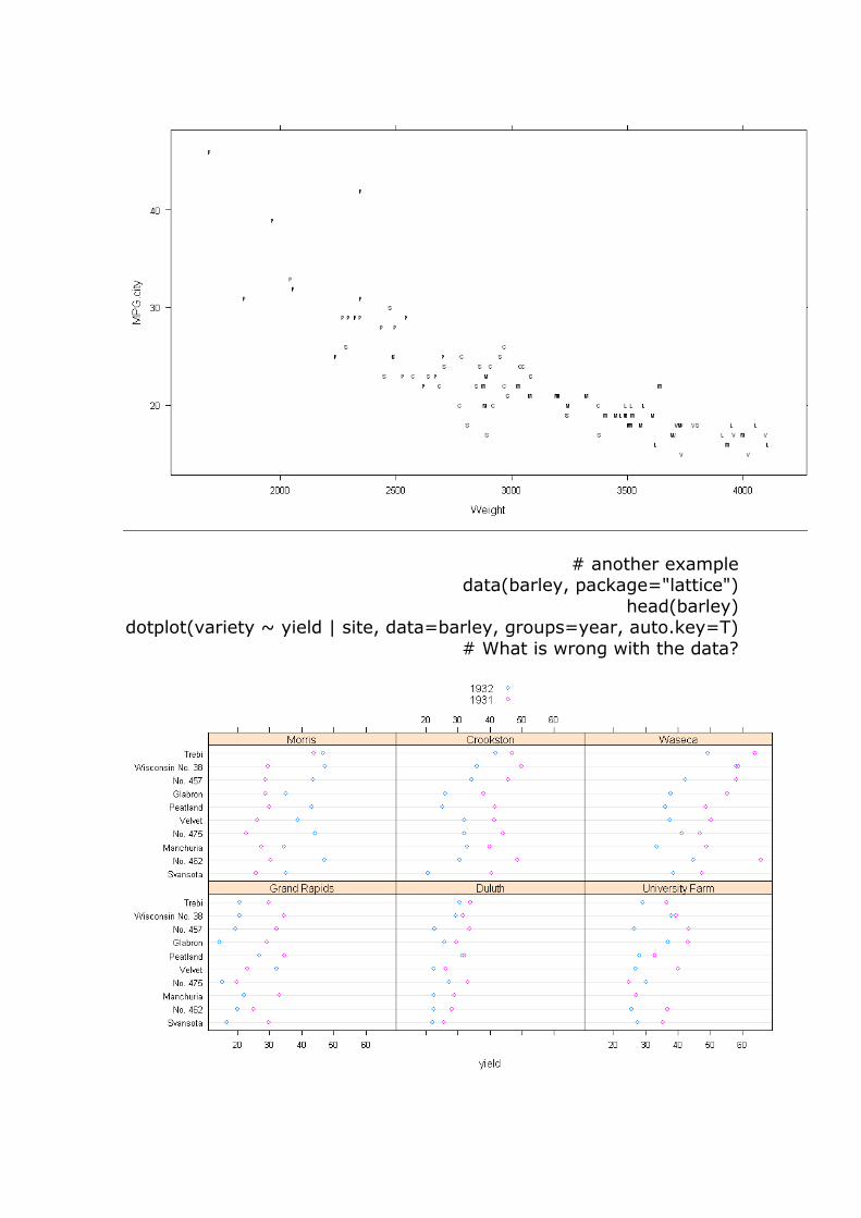
# another example data(barley, package="lattice")
head(barley) dotplot(variety ~ yield | site, data=barley, groups=year, auto.key=T)
# What is wrong with the data?
Page 55
gplots Package
Confidence Intervals - barplot2 I was asked how to plot error bars on a bar chart. This is a somple
question, but I could not find options to add error bars. After some
searching, I fund that a function was available in the Harrell Miscellaneous (Hmisc) package. However, it did not produce as good
charts as I would like. On the call, someone suggested that I look at the gplots package. That package has many useful plots, as well as
an extension to barplot with error bars. gplots needs to be installed by clicking on "Packages" from the R console. There a number of
steps, but you can write a function to combine them. This experience demonstrats both the weakness and strength of R. It is hard to find
where to find the function you are looking for, but with the large number of functions it is probably there somewhere. Also, it is easy
to extend R by writing functions, but it takes some knowledge of the S statistical language.
data(possum, package="DAAG") attach(possum)
head(possum)
library(gplots) conf=0.95 # set argument values so you can step through the
function by submitting individual statements resp=totlngth
cond=sex confInt = function(resp,cond,conf=0.95)
{ x=data.frame(resp,cond);
x=na.omit(x); means=tapply(x$resp,x$cond,mean);
sd=tapply(x$resp,x$cond,sd); n=tapply(x$resp,x$cond,length);
se=sd/sqrt(n); delta=se*qt((1+conf)/2,df=n-1);
data.frame(means=means,lower=means-
delta,upper=means+delta); }
ci=confInt(totlngth,sex); ci ?barplot2
barplot2(ci$means,names.arg=c("Female","Male"),plot.ci=T,ci.l=ci$lower,ci.u=ci$upper)
#note also bargraph.CI(sex,totlngth) # in sciplot package provides se error bars
Page 56
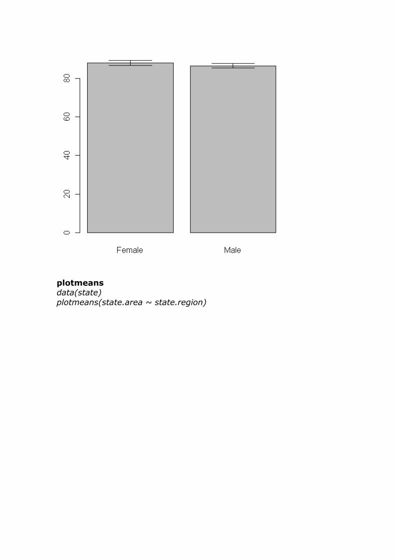
plotmeans data(state)
plotmeans(state.area ~ state.region)
Page 57
plotmeans(state.area ~ state.region, mean.labels=TRUE, digits=-3,
connect=FALSE)
Page 58
balloonplot library(MASS)
data(Cars93) attach(Cars93)
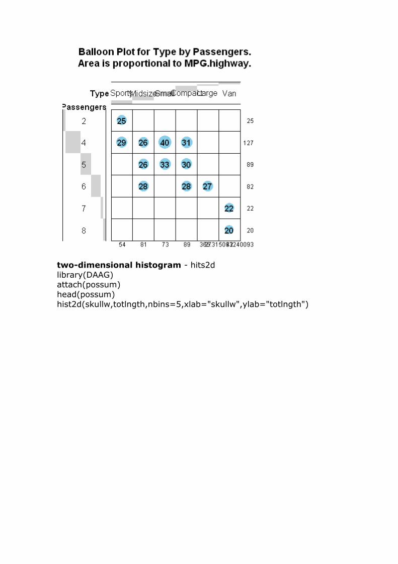
head(Cars93) balloonplot(Type,Passengers,MPG.highway,fun=mean)
Page 59
two-dimensional histogram - hits2d
library(DAAG) attach(possum)
head(possum)
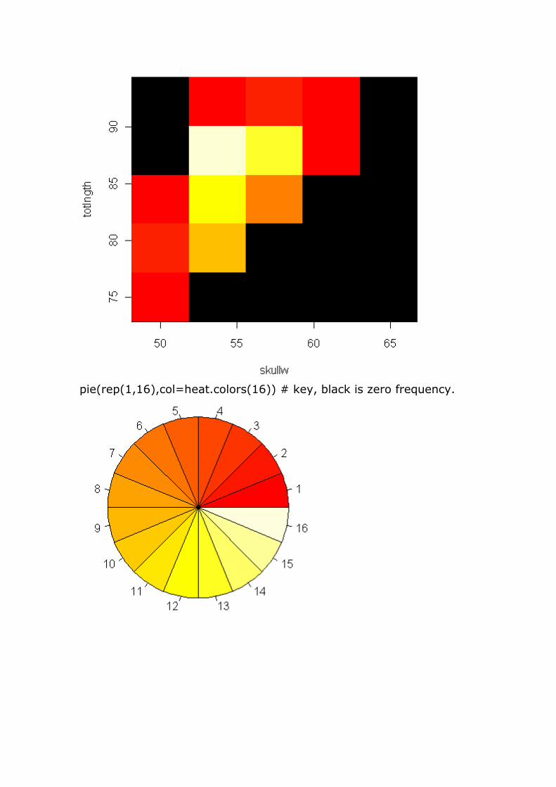
hist2d(skullw,totlngth,nbins=5,xlab="skullw",ylab="totlngth")
Page 60
pie(rep(1,16),col=heat.colors(16)) # key, black is zero frequency.
Page 61
Learn R R is a free software environment for statistical computing and
graphics.
http://www.r-project.org/ Home | Getting Started | Schedule | References | FAQ | Discussion |
Tom's site | Other Courses For more information, please contact Paul Geissler
([email protected] ). Previous page
Topic 12 - Generalized Additive
Models and Mixed-effects Models, Crawley (2007)
Chapters 18, and 19 Chapter 18, Generalized Additive Models Generalized Additive Models (GAMs) provide nonparametric
smoothing. They allow you to view the shape of the relationship, without prejudging the particular parametric form.
Nonparametric smooths like lowess (locally weighted scatterplot smoothing) fit a smooth curve to data by fitting simple models to
localized subsets of the data. #### nonparametric smoothers #####################################
page 612
rm(list = ls()) # removes previous variables
d=read.table("http://www.bio.ic.ac.uk/research/mjcraw/therbook/data/so
aysheep.txt",header=T); attach(d); d
# Year Population Delta # Population N(t) and Delta =
log(N(t+1)/N(t))
# 1 1955 710 0.087598059
# . . .
# 44 1998 1968 -0.746367877
# 45 1999 933 NA # Delta is not defined for last
year.
m=loess(Delta~Population); summary(m) # Wilipedia
# Number of Observations: 44
# Equivalent Number of Parameters: 4.66
# Residual Standard Error: 0.2616 # residual variance = 0.2616^2 =
0.068
# Trace of smoother matrix: 5.11
# Control settings:
# normalize: TRUE
# span : 0.75
# degree : 2
# family : gaussian
# surface : interpolate cell = 0.2
xv=seq(min(Population),max(Population),1);
yv=predict(m,data.frame(Population=xv))
plot(Population,Delta); lines(xv,yv)
Page 62
# Looks like a step function, so use tree to find the split.
library(tree)
m1=tree(Delta~Population); print(m1)
# node), split, n, deviance, yval
# * denotes terminal node
# 1) root 44 5.2870 0.006208
# 2) Population < 1289.5 25 0.8596 0.226500
# 4) Population < 1009.5 13 0.2364 0.277600 *
# 5) Population > 1009.5 12 0.5525 0.171200
# 10) Population < 1059.5 5 0.1631 0.072120 *
# 11) Population > 1059.5 7 0.3053 0.241900 *
# 3) Population > 1289.5 19 1.6180 -0.283700
# 6) Population < 1459 9 0.7917 -0.349500 *
# 7) Population > 1459 10 0.7519 -0.224400 *
th=1289.5; m2=aov(Delta~(Population>th)); summary(m2)
# Df Sum Sq Mean Sq F value Pr(>F)
# Population > 1289.5 1 2.80977 2.80977 47.636 2.008e-08 ***
# Residuals 42 2.47736 0.05898 # loess RMS = 0.068
m=tapply(Delta[!is.na(Delta)],(Population[!is.na(Delta)]>th),mean); m
# FALSE TRUE
# 0.2265084 -0.2836616
plot(Population,Delta); lines(xv,yv)
lines (c(min(Population),th),c(m[1],m[1]),lty=2)
lines (c(th,max(Population)),c(m[2],m[2]),lty=2)
lines (c(th,th),c(m[1],m[2]),lty=2)
#### generalized additive models ############################## page
614
rm(list = ls()) # removes previous variables
d=read.table("http://www.bio.ic.ac.uk/research/mjcraw/therbook/data/oz
one.data.txt",header=T); attach(d); d
# rad temp wind ozone
# 1 190 67 7.4 41
# . . .
pairs(d,panel=function(x,y){ points(x,y);lines(lowess(x,y)) })
library(mgcv)
m1=gam(ozone~s(rad)+s(temp)+s(wind)); summary(m1)
# Family: gaussian
# Link function: identity
# Parametric coefficients:
# Estimate Std. Error t value Pr(>|t|)
# (Intercept) 42.10 1.66 25.36 <2e-16 ***
# Approximate significance of smooth terms:
# edf Ref.df F p-value
# s(rad) 2.763 3.263 4.106 0.00699 **
# s(temp) 3.841 4.341 12.785 7.31e-09 ***
# s(wind) 2.918 3.418 14.687 1.21e-08 ***
# R-sq.(adj) = 0.724 Deviance explained = 74.8%
# GCV score = 338 Scale est. = 305.96 n = 111
m2=gam(ozone~s(temp)+s(wind)); summary(m2) # without s(rad)
anova(m1,m2,test="F")
# Analysis of Deviance Table
# Model 1: ozone ~ s(rad) + s(temp) + s(wind)
# Model 2: ozone ~ s(temp) + s(wind)
# Resid. Df Resid. Dev Df Deviance F Pr(>F)
Page 63
# 1 100.4779 30742
# 2 102.8450 34885 -2.3672 -4142 5.7192 0.002696 ** # s(rad)
should stay in the model
m3=gam(ozone~s(rad)+s(temp)+s(wind)+s(rad,temp)+s(rad,wind)+s(temp,win
d)); summary(m3)
# Parametric coefficients:
# Estimate Std. Error t value Pr(>|t|)
# (Intercept) 42.099 1.286 32.73 <2e-16 ***
# Approximate significance of smooth terms:
# edf Ref.df F p-value
# s(rad) 1.000e+00 1.500 0.001 0.996495
# s(temp) 1.000e+00 1.500 0.010 0.971831
# s(wind) 5.222e+00 5.722 2.115 0.063953 .
# s(rad,temp) 7.963e+00 8.463 1.219 0.298032
# s(rad,wind) 4.144e-10 0.500 1.21e-11 0.998548
# s(temp,wind) 1.830e+01 18.801 2.935 0.000478 ***
m4=gam(ozone~s(rad)+s(temp)+s(wind)+s(temp,wind)); summary(m4)
# Parametric coefficients:
# Estimate Std. Error t value Pr(>|t|)
# (Intercept) 42.099 1.361 30.92 <2e-16 ***
# Approximate significance of smooth terms:
# edf Ref.df F p-value
# s(rad) 1.389 1.889 4.669 0.013368 *
# s(temp) 1.000 1.500 0.000122 0.998982
# s(wind) 5.613 6.113 2.658 0.020054 *
# s(temp,wind) 18.246 18.746 3.210 0.000131 ***
anova(m3,m4,test="F")
# Analysis of Deviance Table
# Model 1: ozone ~ s(rad) + s(temp) + s(wind) + s(rad, temp) + s(rad,
wind) + s(temp, wind)
# Model 2: ozone ~ s(rad) + s(temp) + s(wind) + s(temp, wind)
# Resid. Df Resid. Dev Df Deviance F Pr(>F)
# 1 76.5127 14051.9
# 2 83.7516 17229.7 -7.2389 -3177.8 2.3903 0.02746 *
# Indicates that some other interactions are important, but we will
stay with Crawley's model.
par(mfrow=c(2,2));plot(m4,residuals=T,pch=16);par(mfrow=c(1,1)) #
Rress return in R console (not graph) after each plot.
#### an example with strongly humped data
####################################### page 620
rm(list = ls()) # removes previous variables
library(SemiPar)
data(ethanol); d=ethanol; attach(d); d
# NOx C E # C = compression ratio of engine, E =
equivalance ratio (richness of mixture)
# 1 3.741 12.0 0.907
# . . .
pairs(d,panel=function(x,y){ points(x,y);lines(lowess(x,y)) })
m=gam(NOx~s(E)+C); summary(m) # C looks like a straight line, so use a
parametric fit.
# Parametric coefficients:
# # Estimate Std. Error t value Pr(>|t|)
# (Intercept) 1.291342 0.088898 14.526 < 2e-16 ***
# C 0.055345 0.007062 7.837 1.88e-11 ***
# Approximate significance of smooth terms:
# # edf Ref.df F p-value
Page 64
# s(E) 7.553 8.053 219.6 <2e-16 ***
# R-sq.(adj) = 0.953 Deviance explained = 95.8%
# GCV score = 0.067206 Scale est. = 0.05991 n = 88
par(mfrow=c(1,2));
plot.gam(m,residuals=T,pch=16,all.terms=T);par(mfrow=c(1,1)) # Rress
return in R console (not graph) after each plot.
coplot(NOx~C|E,panel=panel.smooth) # The order of the panel plots is
from the bottom and from the left.
CE=C*E; m2=gam(NOx~s(E)+s(CE)); summary(m2)
# Parametric coefficients:
# Estimate Std. Error t value Pr(>|t|)
# (Intercept) 1.95738 0.02126 92.07 <2e-16 ***
# Approximate significance of smooth terms:
# edf Ref.df F p-value
# s(E) 7.636 8.136 282.52 < 2e-16 ***
# s(CE) 4.261 4.761 27.71 2.02e-15 ***
# R-sq.(adj) = 0.969 Deviance explained = 97.3%
# GCV score = 0.0466 Scale est. = 0.039771 n = 88
par(mfrow=c(1,2));
plot.gam(m,residuals=T,pch=16,all.terms=T);par(mfrow=c(1,1)) # Rress
return in R console (not graph) after each plot.
#### generalized additive models with binary data
########################### page 623
rm(list = ls()) # removes previous variables
d=read.table("http://www.bio.ic.ac.uk/research/mjcraw/therbook/data/is
olation.txt",header=T); attach(d); d
# incidence area isolation # incidence =1 if island occupied by a
bird spedies, =0 if not.
# 1 1 7.928 3.317 # area of island (km2). isolation is
distance from mainland (km)
# 2 0 1.925 7.554
# . . .
m1=gam(incidence~s(area)+s(isolation),binomial); summary(m1)
# Parametric coefficients:
# Estimate Std. Error z value Pr(>|z|)
# (Intercept) 1.6371 0.9898 1.654 0.0981 .
# Approximate significance of smooth terms:
# edf Ref.df Chi.sq p-value
# s(area) 2.429 2.929 3.57 0.3009
# s(isolation) 1.000 1.500 7.48 0.0132 *
# R-sq.(adj) = 0.63 Deviance explained = 63.1%
# UBRE score = -0.32096 Scale est. = 1 n = 50
par(mfrow=c(1,2));
plot.gam(m1,residuals=T,pch=16,all.terms=T);par(mfrow=c(1,1)) # Rress
return in R console (not graph) after each plot.
# Although area in not significant it appears to have a strong effect.
m2=gam(incidence~s(isolation),binomial); anova(m1,m2,test="Chi") #
without area
# Analysis of Deviance Table
# Model 1: incidence ~ s(area) + s(isolation)
# Model 2: incidence ~ s(isolation)
# Resid. Df Resid. Dev Df Deviance P(>|Chi|)
Page 65
# 1 45.5710 25.094
# 2 48.0000 36.640 -2.4290 -11.546 0.005 # significant -
leave s(area) in model
# Note that s(area) was not significant by itself, but made a
significant contribution to the model!
m3=gam(incidence~area+s(isolation),binomial); summary(m3) # fit
parametric area
# Parametric coefficients:
# Estimate Std. Error z value Pr(>|z|)
# (Intercept) -1.3928 0.9002 -1.547 0.1218
# area 0.5807 0.2478 2.344 0.0191 * # highly
significant as parametric, but not as smooth!
# Approximate significance of smooth terms:
# edf Ref.df Chi.sq p-value
# s(isolation) 1 1.5 8.275 0.0087 **
# R-sq.(adj) = 0.597 Deviance explained = 58.3%
# UBRE score = -0.31196 Scale est. = 1 n = 50
Chapter 19, Mixed-Effects Models
Fixed Effects Random Effects
All levels of interest are
studied.
Levels are a random sample from a
larger population.
Influence only the response mean.
Influence only the response variance.
Informative factor levels. Levels not informative.
Examples Examples
age group litter
sex sample plot
treatment individual animals
J. Neter, M. H. Kutner, C. J. Nachtsheim and W. Wasserman (1996, Applied Linear Statistical Models, Irwin, page 959) have pointed out
that for example if a company has five stores and all stores are
included in the sample that stores would be a fixed effect. However, if the company had hundreds of stores and a random sample of five
stores were included in the sample, then stores would be a random effect. Thus it is the nature of the sample and the inferences one
wants to draw that determine whether an effect is fixed or random. Assumptions:
• Within-group defined by the fixed effect, errors are independent with mean 0 and variance σ2.
• Within-group defined by the fixed effect, errors are independent of the random effects.
• Random effects are normally distributed with mean 0 and covariance matrix Ψ
• The random effects are independent in different groups. • The covariance matrix does not depend on the group defined by the
fixed effects.
Page 66
Replicates: • must be independent
• must not be repeated measurements or time series (temporal
pseudoreplication) • must not be grouped together in one place (spatial
pseudoreplication)
When you have a hierarchical model (pseudoreplication), you can: • Remove the pseudoreplication by analyzing the mean or other
function of the dependent observations. • Analyze each group with pseudoreplication separately.
• Use mixed effects models or time series analysis. #### split plots ##################################### page 632
rm(list = ls()) # removes previous variables
d=read.table("http://www.bio.ic.ac.uk/research/mjcraw/therbook/data/sp
lityield.txt",header=T); attach(d); d
# yield block irrigation density fertilizer
# 1 90 A control low N
# . . .
# block: Blocks (whole fields) are the largest areas
# irrigation: Blocks were split in half and irrigation treatments were
applies to half of each field.
# density: Irrigation plots were split into thirds and seeds sown at
three densities (low, medium and high).
# fertilizer: Density plots were split into thirds and fertilizer
treatments applied (N, P and NP).
library(nlme) # You may need to install nlme
?lme
m=lme(yield~irrigation*density*fertilizer,random=~1|block/irrigation/d
ensity); summary(m)
# Linear mixed-effects model fit by REML
# Data: NULL
# AIC BIC logLik
# 481.6212 525.3789 -218.8106
# Random effects:
# Formula: ~1 | block
# (Intercept)
# StdDev: 0.0006600339
# Formula: ~1 | irrigation %in% block
# (Intercept)
# StdDev: 1.982461
# Formula: ~1 | density %in% irrigation %in% block
# (Intercept) Residual
# StdDev: 6.975554 9.292805
# Fixed effects: yield ~ irrigation * density * fertilizer
# Value
Std.Error DF t-value p-value
# (Intercept) 80.50
5.893741 36 13.658558 0.0000
# irrigation[T.irrigated] 31.75
8.335008 3 3.809234 0.0318
# density[T.low] 5.50
8.216282 12 0.669403 0.5159
# density[T.medium] 14.75
8.216282 12 1.795216 0.0978
Page 67
# fertilizer[T.NP] 5.50
6.571005 36 0.837010 0.4081
# fertilizer[T.P] 4.50
6.571005 36 0.684827 0.4978
# irrigation[T.irrigated]:density[T.low] -39.00
11.619577 12 -3.356404 0.0057
# irrigation[T.irrigated]:density[T.medium] -22.25
11.619577 12 -1.914872 0.0796
# irrigation[T.irrigated]:fertilizer[T.NP] 13.00
9.292805 36 1.398932 0.1704
# irrigation[T.irrigated]:fertilizer[T.P] 5.50
9.292805 36 0.591856 0.5576
# density[T.low]:fertilizer[T.NP] 3.25
9.292805 36 0.349733 0.7286
# density[T.medium]:fertilizer[T.NP] -6.75
9.292805 36 -0.726368 0.4723
# density[T.low]:fertilizer[T.P] -5.25
9.292805 36 -0.564953 0.5756
# density[T.medium]:fertilizer[T.P] -5.50
9.292805 36 -0.591856 0.5576
# irrigation[T.irrigated]:density[T.low]:fertilizer[T.NP] 7.75
13.142011 36 0.589712 0.5591
# irrigation[T.irrigated]:density[T.medium]:fertilizer[T.NP] 3.75
13.142011 36 0.285344 0.7770
# irrigation[T.irrigated]:density[T.low]:fertilizer[T.P] 20.00
13.142011 36 1.521837 0.1368
# irrigation[T.irrigated]:density[T.medium]:fertilizer[T.P] 4.00
13.142011 36 0.304367 0.7626
# Correlation: omitted because they are too wide
# Standardized Within-Group Residuals:
# Min Q1 Med Q3 Max
# -2.12362041 -0.37841447 -0.03057733 0.41805004 1.90433189
# Number of Observations: 72
# Number of Groups:
# block irrigation %in%
block density %in% irrigation %in% block
# 4
8 24
## use maximum likelihood (ML) instead of default restricted maximum
likelihood (REML) so we can use anova
## Restricted maximum likelihood (REML) allows for degrees of freedom
to be used up in estimating fixed effects,
## unlike maximum likelihood (ML).
## Thus variance components are estimated without being affected by
the fixed effects.
## REML estimators are less sensitive to outliers than ML estimators.
m1=lme(yield~irrigation*density*fertilizer,random=~1|block/irrigation/
density,method="ML");summary(m1);anova(m1)
# summary gives the same results
# numDF denDF F-value p-value
# (Intercept) 1 36 2674.6630 <.0001
# irrigation 1 3 30.9211 0.0115
# density 2 12 3.7842 0.0532
# fertilizer 2 36 11.4493 0.0001
# irrigation:density 2 12 5.9119 0.0163
# irrigation:fertilizer 2 36 5.5204 0.0081
# density:fertilizer 4 36 0.8826 0.4841
# irrigation:density:fertilizer 4 36 0.6795 0.6107
Page 68
m2=lme(yield~(irrigation+density+fertilizer)^2,random=~1|block/irrigat
ion/density,method="ML")# remove higher order interactions
anova(m2)
# numDF denDF F-value p-value
# (Intercept) 1 40 2872.7394 <.0001
# irrigation 1 3 33.2110 0.0104
# density 2 12 4.0645 0.0449
# fertilizer 2 40 11.4341 0.0001
# irrigation:density 2 12 6.3499 0.0132
# irrigation:fertilizer 2 40 5.5131 0.0077
# density:fertilizer 4 40 0.8815 0.4837
anova(m1,m2)
# Model df AIC BIC logLik Test L.Ratio p-value
# m1 1 22 573.5108 623.5974 -264.7554
# m2 2 18 569.0046 609.9845 -266.5023 1 vs 2 3.493788 0.4788 # m2
better
m3=update(m2,~.-density:fertilizer); anova(m3)
# numDF denDF F-value p-value
# (Intercept) 1 44 3070.8771 <.0001
# irrigation 1 3 35.5016 0.0095
# density 2 12 4.3448 0.0381
# fertilizer 2 44 11.2013 0.0001
# irrigation:density 2 12 6.7878 0.0107
# irrigation:fertilizer 2 44 5.4008 0.0080
anova(m2,m3)
# Model df AIC BIC logLik Test L.Ratio p-value
# m2 1 18 569.0046 609.9845 -266.5023
# m3 2 14 565.1933 597.0667 -268.5967 1 vs 2 4.188774 0.3811
## m3 not significantly different, and gives lower AIC and BIC so use
m3
m4=update(m3,~.-irrigation:fertilizer); anova(m4)
# numDF denDF F-value p-value
# (Intercept) 1 46 3169.893 <.0001
# irrigation 1 3 36.646 0.0090
# density 2 12 4.485 0.0351
# fertilizer 2 46 9.167 0.0004
# irrigation:density 2 12 7.007 0.0096
anova(m3,m4)
# Model df AIC BIC logLik Test L.Ratio p-value
# m3 1 14 565.1933 597.0667 -268.5967
# m4 2 12 572.3373 599.6573 -274.1687 1 vs 2 11.14397 0.0038
## m4 is significantly different and gives a larger AIC and BIC, so
keep m3
m5=update(m3,~.-irrigation:density); anova(m5)
# numDF denDF F-value p-value
# (Intercept) 1 44 2138.9678 <.0001
# irrigation 1 3 24.7281 0.0156
# density 2 14 2.6264 0.1075
# fertilizer 2 44 11.5626 0.0001
# irrigation:fertilizer 2 44 5.5750 0.0069
anova(m3,m5)
# Model df AIC BIC logLik Test L.Ratio p-value
# m3 1 14 565.1933 597.0667 -268.5967
# m5 2 12 572.9022 600.2221 -274.4511 1 vs 2 11.70883 0.0029
## m5 is significantly different and gives a larger AIC and BIC, so
keep m3
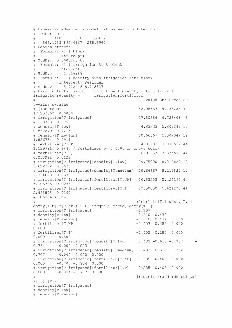
summary(m3); anova(m3)
Page 69
# Linear mixed-effects model fit by maximum likelihood
# Data: NULL
# AIC BIC logLik
# 565.1933 597.0667 -268.5967
# Random effects:
# Formula: ~1 | block
# (Intercept)
# StdDev: 0.0005260787
# Formula: ~1 | irrigation %in% block
# (Intercept)
# StdDev: 1.716888
# Formula: ~1 | density %in% irrigation %in% block
# (Intercept) Residual
# StdDev: 5.722413 8.718327
# Fixed effects: yield ~ irrigation + density + fertilizer +
irrigation:density + irrigation:fertilizer
# Value Std.Error DF
t-value p-value
# (Intercept) 82.08333 4.756285 44
17.257867 0.0000
# irrigation[T.irrigated] 27.80556 6.726403 3
4.133793 0.0257
# density[T.low] 4.83333 5.807347 12
0.832279 0.4215
# density[T.medium] 10.66667 5.807347 12
1.836754 0.0911
# fertilizer[T.NP] 4.33333 3.835552 44
1.129781 0.2647 # fertilizer p= 0.0001 in anova below
# fertilizer[T.P] 0.91667 3.835552 44
0.238992 0.8122
# irrigation[T.irrigated]:density[T.low] -29.75000 8.212829 12 -
3.622382 0.0035
# irrigation[T.irrigated]:density[T.medium] -19.66667 8.212829 12 -
2.394628 0.0338
# irrigation[T.irrigated]:fertilizer[T.NP] 16.83333 5.424290 44
3.103325 0.0033
# irrigation[T.irrigated]:fertilizer[T.P] 13.50000 5.424290 44
2.488805 0.0167
# Correlation:
# (Intr) ir[T.] dnsty[T.l]
dnsty[T.m] f[T.NP f[T.P] irrgtn[T.rrgtd]:dnsty[T.l]
# irrigation[T.irrigated] -0.707
# density[T.low] -0.610 0.432
# density[T.medium] -0.610 0.432 0.500
# fertilizer[T.NP] -0.403 0.285 0.000
0.000
# fertilizer[T.P] -0.403 0.285 0.000
0.000 0.500
# irrigation[T.irrigated]:density[T.low] 0.432 -0.610 -0.707 -
0.354 0.000 0.000
# irrigation[T.irrigated]:density[T.medium] 0.432 -0.610 -0.354 -
0.707 0.000 0.000 0.500
# irrigation[T.irrigated]:fertilizer[T.NP] 0.285 -0.403 0.000
0.000 -0.707 -0.354 0.000
# irrigation[T.irrigated]:fertilizer[T.P] 0.285 -0.403 0.000
0.000 -0.354 -0.707 0.000
# irrgtn[T.rrgtd]:dnsty[T.m]
i[T.]:[T.N
# irrigation[T.irrigated]
# density[T.low]
# density[T.medium]
Page 70
# fertilizer[T.NP]
# fertilizer[T.P]
# irrigation[T.irrigated]:density[T.low]
# irrigation[T.irrigated]:density[T.medium]
# irrigation[T.irrigated]:fertilizer[T.NP] 0.000
# irrigation[T.irrigated]:fertilizer[T.P] 0.000
0.500
# Standardized Within-Group Residuals:
# Min Q1 Med Q3 Max
# -2.58166961 -0.51480885 0.07893406 0.60157076 2.19570825
# Number of Observations: 72
# Number of Groups:
# block irrigation %in%
block density %in% irrigation %in% block
# 4
8 24
anova(m3)
# numDF denDF F-value p-value
# (Intercept) 1 44 3070.8771 <.0001 # note
differences in denDF
# irrigation 1 3 35.5016 0.0095 # due to split
plots
# density 2 12 4.3448 0.0381
# fertilizer 2 44 11.2013 0.0001
# irrigation:density 2 12 6.7878 0.0107
# irrigation:fertilizer 2 44 5.4008 0.0080
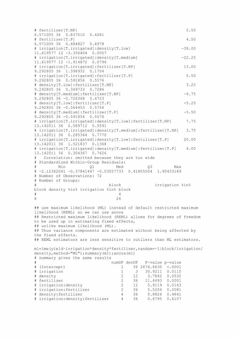
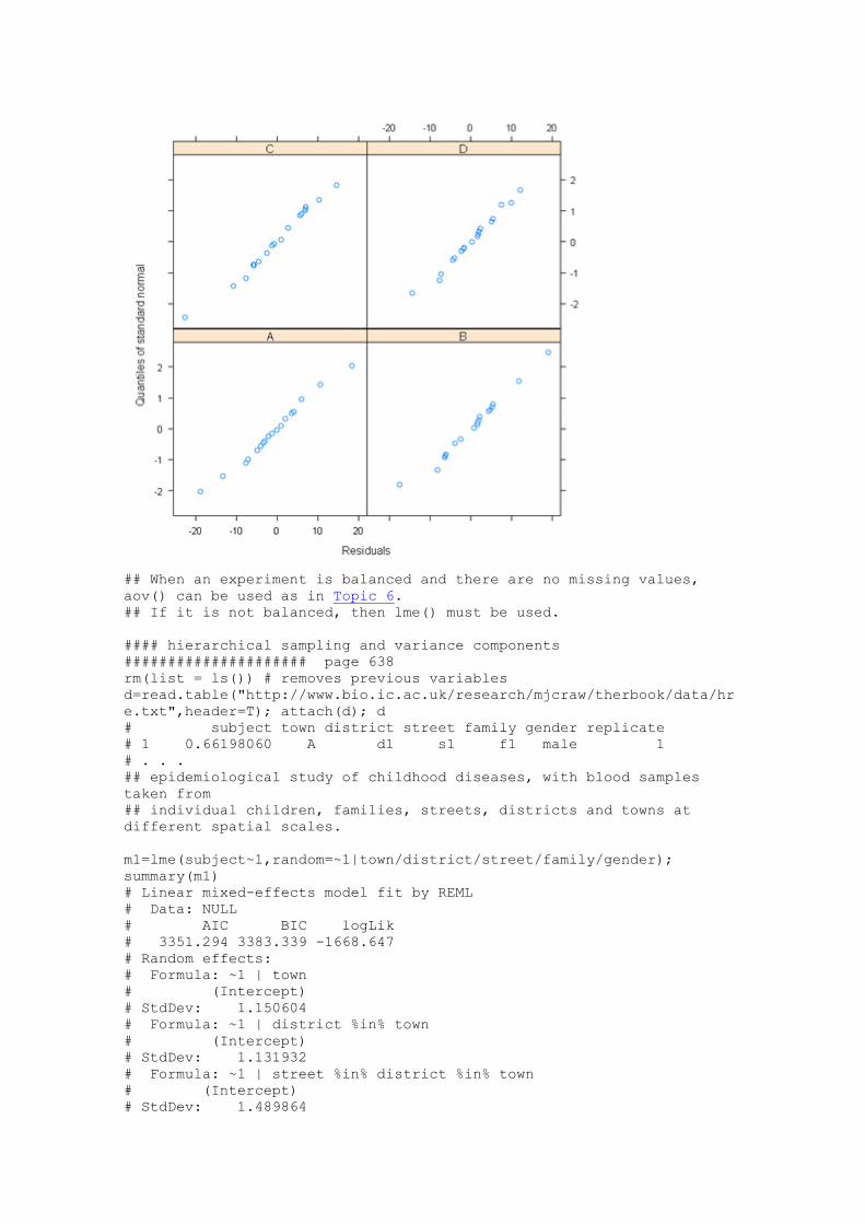
## In R console set history > recording after plot
plot(m3);plot(m3,yield~fitted(.)); qqnorm(m3,~resid(.)|block)
Page 71
## When an experiment is balanced and there are no missing values,
aov() can be used as in Topic 6.
## If it is not balanced, then lme() must be used.
#### hierarchical sampling and variance components
##################### page 638
rm(list = ls()) # removes previous variables
d=read.table("http://www.bio.ic.ac.uk/research/mjcraw/therbook/data/hr
e.txt",header=T); attach(d); d
# subject town district street family gender replicate
# 1 0.66198060 A d1 s1 f1 male 1
# . . .
## epidemiological study of childhood diseases, with blood samples
taken from
## individual children, families, streets, districts and towns at
different spatial scales.
m1=lme(subject~1,random=~1|town/district/street/family/gender);
summary(m1)
# Linear mixed-effects model fit by REML
# Data: NULL
# AIC BIC logLik
# 3351.294 3383.339 -1668.647
# Random effects:
# Formula: ~1 | town
# (Intercept)
# StdDev: 1.150604
# Formula: ~1 | district %in% town
# (Intercept)
# StdDev: 1.131932
# Formula: ~1 | street %in% district %in% town
# (Intercept)
# StdDev: 1.489864
Page 72
# Formula: ~1 | family %in% street %in% district %in% town
# (Intercept)
# StdDev: 1.923191
# Formula: ~1 | gender %in% family %in% street %in% district %in%
town
# (Intercept) Residual
# StdDev: 3.917264 0.9245321
# Fixed effects: subject ~ 1
# Value Std.Error DF t-value p-value
# (Intercept) 8.010941 0.6719753 360 11.92148 0
# Standardized Within-Group Residuals:
# Min Q1 Med Q3 Max
# -2.64600654 -0.47626815 -0.06009422 0.47531635 2.35647504
# Number of Observations: 720
# Number of Groups:
# town
district %in% town
# 5
15
# street %in% district %in% town
family %in% street %in% district %in% town
# 60
180
# gender %in% family %in% street %in% district %in% town
# 360
## variance components from StdDev above. I can't get them from m1 or
s1 using statements.
v=c(1.150604, 1.131932, 1.489864, 1.923191, 3.917264, 0.9245321)^2
names(v)=c("town","district","street","family","gender","residual");v
# town district street family gender residual
# 1.3238896 1.2812701 2.2196947 3.6986636 15.3449572 0.8547596
v/sum(v)*100 # percent
# town district street family gender residual
# 5.354840 5.182453 8.978173 14.960274 62.066948 3.457313
## Restricted maximum likelihood (REML) allows for degrees of freedom
to be used up in estimating fixed effects,
## unlike maximum likelihood (ML).
## Thus variance components are estimated without being affected by
the fixed effects.
## REML estimators are less sensitive to outliers than ML estimators.
#### using lmer
library(lme4)
?lmer
m2=lmer(subject~1 + (1|town/district/street/family/gender));
summary(m2)
# Linear mixed model fit by REML
# Formula: subject ~ 1 + (1 | town/district/street/family/gender)
# AIC BIC logLik deviance REMLdev
# 3351 3383 -1669 3338 3337
# Random effects: ## gives variance
components ##
# Groups Name Variance
Std.Dev.
# gender:(family:(street:(district:town))) (Intercept) 15.34509
3.91728
# family:(street:(district:town)) (Intercept) 3.69852
1.92315
# street:(district:town) (Intercept) 2.21970
1.48987
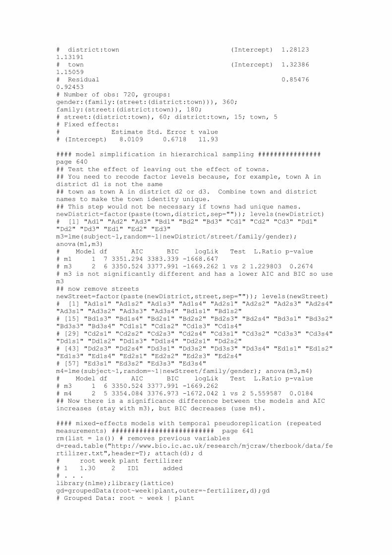
Page 73
# district:town (Intercept) 1.28123
1.13191
# town (Intercept) 1.32386
1.15059
# Residual 0.85476
0.92453
# Number of obs: 720, groups:
gender:(family:(street:(district:town))), 360;
family:(street:(district:town)), 180;
# street:(district:town), 60; district:town, 15; town, 5
# Fixed effects:
# Estimate Std. Error t value
# (Intercept) 8.0109 0.6718 11.93
#### model simplification in hierarchical sampling ################
page 640
## Test the effect of leaving out the effect of towns.
## You need to recode factor levels because, for example, town A in
district d1 is not the same
## town as town A in district d2 or d3. Combine town and district
names to make the town identity unique.
## This step would not be necessary if towns had unique names.
newDistrict=factor(paste(town,district,sep="")); levels(newDistrict)
# [1] "Ad1" "Ad2" "Ad3" "Bd1" "Bd2" "Bd3" "Cd1" "Cd2" "Cd3" "Dd1"
"Dd2" "Dd3" "Ed1" "Ed2" "Ed3"
m3=lme(subject~1,random=~1|newDistrict/street/family/gender);
anova(m1,m3)
# Model df AIC BIC logLik Test L.Ratio p-value
# m1 1 7 3351.294 3383.339 -1668.647
# m3 2 6 3350.524 3377.991 -1669.262 1 vs 2 1.229803 0.2674
# m3 is not significantly different and has a lower AIC and BIC so use
m3
## now remove streets
newStreet=factor(paste(newDistrict,street,sep="")); levels(newStreet)
# [1] "Ad1s1" "Ad1s2" "Ad1s3" "Ad1s4" "Ad2s1" "Ad2s2" "Ad2s3" "Ad2s4"
"Ad3s1" "Ad3s2" "Ad3s3" "Ad3s4" "Bd1s1" "Bd1s2"
# [15] "Bd1s3" "Bd1s4" "Bd2s1" "Bd2s2" "Bd2s3" "Bd2s4" "Bd3s1" "Bd3s2"
"Bd3s3" "Bd3s4" "Cd1s1" "Cd1s2" "Cd1s3" "Cd1s4"
# [29] "Cd2s1" "Cd2s2" "Cd2s3" "Cd2s4" "Cd3s1" "Cd3s2" "Cd3s3" "Cd3s4"
"Dd1s1" "Dd1s2" "Dd1s3" "Dd1s4" "Dd2s1" "Dd2s2"
# [43] "Dd2s3" "Dd2s4" "Dd3s1" "Dd3s2" "Dd3s3" "Dd3s4" "Ed1s1" "Ed1s2"
"Ed1s3" "Ed1s4" "Ed2s1" "Ed2s2" "Ed2s3" "Ed2s4"
# [57] "Ed3s1" "Ed3s2" "Ed3s3" "Ed3s4"
m4=lme(subject~1,random=~1|newStreet/family/gender); anova(m3,m4)
# Model df AIC BIC logLik Test L.Ratio p-value
# m3 1 6 3350.524 3377.991 -1669.262
# m4 2 5 3354.084 3376.973 -1672.042 1 vs 2 5.559587 0.0184
## Now there is a significance difference between the models and AIC
increases (stay with m3), but BIC decreases (use m4).
#### mixed-effects models with temporal pseudoreplication (repeated
measurements) ########################## page 641
rm(list = ls()) # removes previous variables
d=read.table("http://www.bio.ic.ac.uk/research/mjcraw/therbook/data/fe
rtilizer.txt",header=T); attach(d); d
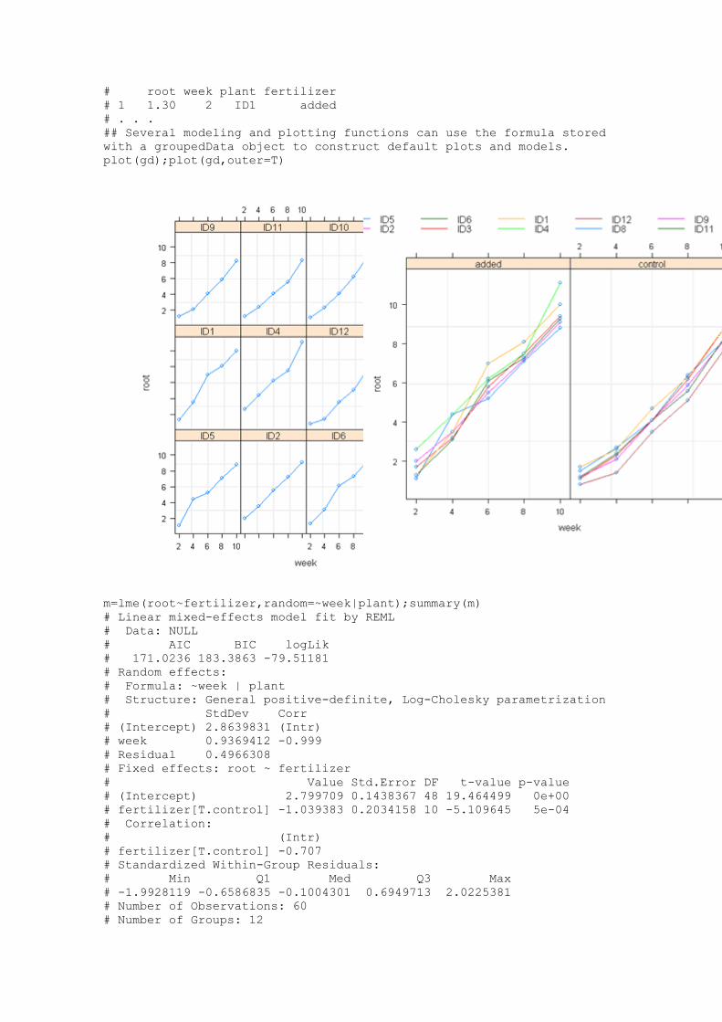
# root week plant fertilizer
# 1 1.30 2 ID1 added
# . . .
library(nlme);library(lattice)
gd=groupedData(root~week|plant,outer=~fertilizer,d);gd
# Grouped Data: root ~ week | plant
Page 74
# root week plant fertilizer
# 1 1.30 2 ID1 added
# . . .
## Several modeling and plotting functions can use the formula stored
with a groupedData object to construct default plots and models.
plot(gd);plot(gd,outer=T)
m=lme(root~fertilizer,random=~week|plant);summary(m)
# Linear mixed-effects model fit by REML
# Data: NULL
# AIC BIC logLik
# 171.0236 183.3863 -79.51181
# Random effects:
# Formula: ~week | plant
# Structure: General positive-definite, Log-Cholesky parametrization
# StdDev Corr
# (Intercept) 2.8639831 (Intr)
# week 0.9369412 -0.999
# Residual 0.4966308
# Fixed effects: root ~ fertilizer
# Value Std.Error DF t-value p-value
# (Intercept) 2.799709 0.1438367 48 19.464499 0e+00
# fertilizer[T.control] -1.039383 0.2034158 10 -5.109645 5e-04
# Correlation:
# (Intr)
# fertilizer[T.control] -0.707
# Standardized Within-Group Residuals:
# Min Q1 Med Q3 Max
# -1.9928119 -0.6586835 -0.1004301 0.6949713 2.0225381
# Number of Observations: 60
# Number of Groups: 12
Page 75
anova(m)
# numDF denDF F-value p-value
# (Intercept) 1 48 502.5360 <.0001
# fertilizer 1 10 26.1085 5e-04
## Two treatments (fertilizers) and 12 plants (6 in each treatment)
## so there are 2(6-1)=10 df for testing fertilizer.
## Without using mixed models, you can test the data for week 10
without repeated measures.
m1=aov(root~fertilizer,subset=(week==10)); summary(m1)
# Df Sum Sq Mean Sq F value Pr(>F)
# fertilizer 1 4.9408 4.9408 11.486 0.006897 **
# Residuals 10 4.3017 0.4302
## Mixed models uses more data and has more power to detect
differences.
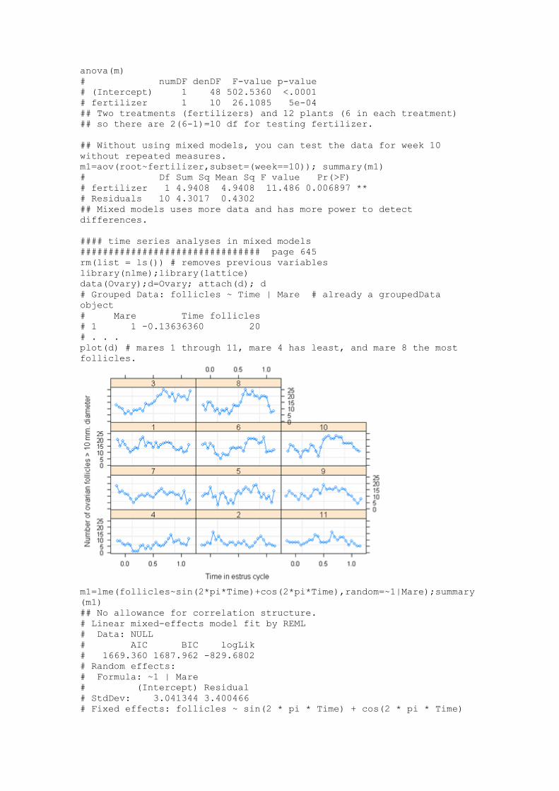
#### time series analyses in mixed models
################################ page 645
rm(list = ls()) # removes previous variables
library(nlme);library(lattice)
data(Ovary);d=Ovary; attach(d); d
# Grouped Data: follicles ~ Time | Mare # already a groupedData
object
# Mare Time follicles
# 1 1 -0.13636360 20
# . . .
plot(d) # mares 1 through 11, mare 4 has least, and mare 8 the most
follicles.
m1=lme(follicles~sin(2*pi*Time)+cos(2*pi*Time),random=~1|Mare);summary
(m1)
## No allowance for correlation structure.
# Linear mixed-effects model fit by REML
# Data: NULL
# AIC BIC logLik
# 1669.360 1687.962 -829.6802
# Random effects:
# Formula: ~1 | Mare
# (Intercept) Residual
# StdDev: 3.041344 3.400466
# Fixed effects: follicles ~ sin(2 * pi * Time) + cos(2 * pi * Time)
Page 76
# Value Std.Error DF t-value p-value
# (Intercept) 12.182244 0.9390009 295 12.973623 0.0000
# sin(2 * pi * Time) -3.339612 0.2894013 295 -11.539727 0.0000
# cos(2 * pi * Time) -0.862422 0.2715987 295 -3.175353 0.0017
# Correlation:
# (Intr) s(*p*T
# sin(2 * pi * Time) 0.00
# cos(2 * pi * Time) -0.06 0.00
# Standardized Within-Group Residuals:
# Min Q1 Med Q3 Max
# -2.4500138 -0.6721813 -0.1349236 0.5922957 3.5506618
# Number of Observations: 308
# Number of Groups: 11 # Mares
plot(ACF(m1),alpha=0.05) # ACF is autocorrelation function
## highly signification autocorrelation at lags 1 and 2; and
marginally significant ones at lags 3 and 4
m2=update(m1,correlation=corARMA(q=2)); anova(m1,m2) # moving average
model with first two lags.
# Model df AIC BIC logLik Test L.Ratio p-value
# m1 1 5 1669.360 1687.962 -829.6802
# m2 2 7 1574.895 1600.937 -780.4476 1 vs 2 98.4652 <.0001
## m2 has lower AIC and BIC and so is preferred.
m3=update(m2,correlation=corAR1()); anova(m2,m3) # First order
autoregressive model
# Model df AIC BIC logLik Test L.Ratio p-value
# m2 1 7 1574.895 1600.937 -780.4476
# m3 2 6 1562.447 1584.769 -775.2233 1 vs 2 10.44840 0.0012
## p value is very different from text but AIC and BIC are the same.
## m3 has lower AIC and BIC and so is preferred.
## Time series analysis is covered in Chapter 22.
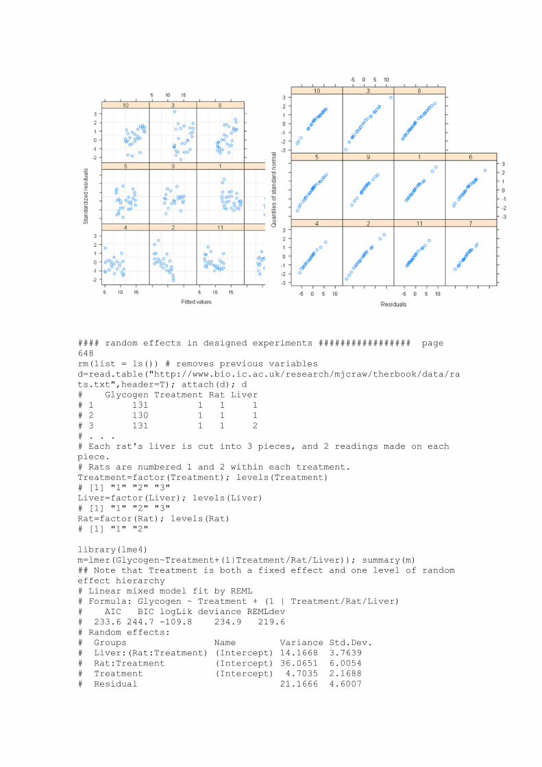
plot(m3,resid(.,type="p")~fitted(.)|Mare); qqnorm(m3,~resid(.)|Mare)
Page 77
#### random effects in designed experiments ################# page
648
rm(list = ls()) # removes previous variables
d=read.table("http://www.bio.ic.ac.uk/research/mjcraw/therbook/data/ra
ts.txt",header=T); attach(d); d
# Glycogen Treatment Rat Liver
# 1 131 1 1 1
# 2 130 1 1 1
# 3 131 1 1 2
# . . .
# Each rat's liver is cut into 3 pieces, and 2 readings made on each
piece.
# Rats are numbered 1 and 2 within each treatment.
Treatment=factor(Treatment); levels(Treatment)
# [1] "1" "2" "3"
Liver=factor(Liver); levels(Liver)
# [1] "1" "2" "3"
Rat=factor(Rat); levels(Rat)
# [1] "1" "2"
library(lme4)
m=lmer(Glycogen~Treatment+(1|Treatment/Rat/Liver)); summary(m)
## Note that Treatment is both a fixed effect and one level of random
effect hierarchy
# Linear mixed model fit by REML
# Formula: Glycogen ~ Treatment + (1 | Treatment/Rat/Liver)
# AIC BIC logLik deviance REMLdev
# 233.6 244.7 -109.8 234.9 219.6
# Random effects:
# Groups Name Variance Std.Dev.
# Liver:(Rat:Treatment) (Intercept) 14.1668 3.7639
# Rat:Treatment (Intercept) 36.0651 6.0054
# Treatment (Intercept) 4.7035 2.1688
# Residual 21.1666 4.6007
Page 78
# Number of obs: 36, groups: Liver:(Rat:Treatment), 18; Rat:Treatment,
6; Treatment, 3
# Fixed effects:
# Estimate Std. Error t value
# (Intercept) 140.500 5.182 27.112
# Treatment[T.2] 10.500 7.329 1.433
# Treatment[T.3] -5.333 7.329 -0.728
# Correlation of Fixed Effects:
# (Intr) T[T.2]
#Trtmnt[T.2] -0.707
#Trtmnt[T.3] -0.707 0.500
anova(m)
# Analysis of Variance Table
# Df Sum Sq Mean Sq F value
# Treatment 2 101.943 50.971 2.4081
v=c(14.1668,36.0651,21.1666); # Treatment is a fixed effect
names(v)=c("liver","rats","readings"); v
# liver rats readings
# 14.1668 36.0651 21.1666
100*v/sum(v) # percent
# liver rats readings
# 19.84187 50.51241 29.64572
#### regression in mixed-effects models ####################### page
650
rm(list = ls()) # removes previous variables
d=read.table("http://www.bio.ic.ac.uk/research/mjcraw/therbook/data/fa
rms.txt",header=T); attach(d); d
# N size farm
# 1 18.18014 96.48147 1
# 2 20.47343 98.64003 1
# . . .
## regression of plant size against local point measurement of soil
nitrogen (N)
## at five places within each of 24 farms.
plot(size~N,pch=16,col=farm)
Page 79
## fit a separate regressions for each farm
m=lmList(size~N|farm,d); c=coef(m); c
# (Intercept) N
# 1 67.46260 1.5153805
# 2 118.52443 -0.5550273
# 3 91.58055 0.5551292
# 4 87.92259 0.9212662
# 5 92.12023 0.5380276
# 6 97.01996 0.3845431
# 7 68.52117 0.9339957
# 8 91.54383 0.8220482
# 9 92.04667 0.8842662
# 10 85.08964 1.4676459
# 11 114.93449 -0.2689370
# 12 82.56263 1.0138488
# 13 78.60940 0.1324811
# 14 80.97221 0.6551149
# 15 84.85382 0.9809902
# 16 87.12280 0.3699154
# 17 52.31711 1.7555136
# 18 83.40400 0.8715070
# 19 88.91675 0.2043755
# 20 93.08216 0.8567066
# 21 90.24868 0.7830692
# 22 78.30970 1.1441291
# 23 59.88093 0.9536750
# 24 89.07963 0.1091016
range(c[,"(Intercept)"])
# [1] 52.31711 118.52443
range(c[,"N"])
# [1] -0.5550273 1.7555136
Page 80
## Now fit a single mixed model, taking into account the differences
between farms
## in their contributions to the variance.
m1=lme(size~1,random=~N|farm); summary(m1);
# Linear mixed-effects model fit by REML
# Data: NULL
# AIC BIC logLik
# 643.4823 657.3779 -316.7411
# Random effects:
# Formula: ~N | farm
# Structure: General positive-definite, Log-Cholesky parametrization
# StdDev Corr
# (Intercept) 12.3857402 (Intr)
# N 0.6215039 -0.735
# Residual 1.9826698
# Fixed effects: size ~ 1
# Value Std.Error DF t-value p-value
# (Intercept) 97.95195 1.810111 96 54.11378 0
#
# Standardized Within-Group Residuals:
# Min Q1 Med Q3 Max
# -2.19364865 -0.56777008 0.04701894 0.64022046 2.01476221
# Number of Observations: 120
# Number of Groups: 24
v=c(12.3857402,0.6215039,1.9826698)^2;
names(v)=c("(Intercept)","N","Residual"); v
# (Intercept) N Residual
# 153.4065603 0.3862671 3.9309795
100*v/sum(v) # percent of variance
# (Intercept) N Residual
# 97.2627806 0.2449009 2.4923184
c1=coef(m1); c1
# (Intercept) N
# 1 85.98140 0.574205232
# 2 104.67366 -0.045401462
# 3 95.03442 0.331080899
# 4 98.62679 0.463579764
# 5 95.00270 0.407906188
# 6 99.82294 0.207203693
# 7 85.57345 0.285520337
# 8 96.09461 0.520896445
# 9 95.22186 0.672262902
# 10 93.14157 1.017995666
# 11 108.27200 0.015213757
# 12 87.36387 0.689406363
# 13 80.83933 0.003616946
# 14 89.84309 0.306402229
# 15 93.37050 0.636778651
# 16 92.10914 0.145772142
# 17 94.93395 0.084935465
# 18 85.90160 0.709943233
# 19 92.00628 0.052485978
# 20 95.26296 0.738029377
# 21 93.35069 0.591151930
# 22 87.66161 0.673119211
# 23 70.57827 0.432993864
# 24 90.29151 0.036747095
par(mfrow=c(1,2));
plot(c[,"(Intercept)"],c1[,"(Intercept)"],main="Intercept",xlab="separ
ate regressions",ylab="mixed model")
abline(0,1)
Page 81
plot(c[,"N"],c1[,"N"],main="Slope",xlab="separate
regressions",ylab="mixed model")
abline(0,1)
par(mfrow=c(1,1));
farm=factor(farm)
## N and farm as fixed effects
## Use ML to compare models with anova()
m2=lme(size~N*farm,random=~1|farm,method="ML") # full model
m3=lme(size~N+farm,random=~1|farm,method="ML") # common slope,
different intercepts
m4=lme(size~N,random=~1|farm,method="ML") # common slope and
intercept
m5=lme(size~1,random=~1|farm,method="ML") # no effect of N
anova(m2,m3,m4,m5)
# Model df AIC BIC logLik Test L.Ratio p-value
# m2 1 50 542.9035 682.2781 -221.4518
# m3 2 27 524.2971 599.5594 -235.1486 1 vs 2 27.39359 0.2396
# m4 3 4 614.3769 625.5269 -303.1885 2 vs 3 136.07981 <.0001
# m5 4 3 658.0058 666.3683 -326.0029 3 vs 4 45.62892 <.0001
## m3 has lowest AIC and BIC and is not significantly different from
m2
summary(m3)
# Linear mixed-effects model fit by maximum likelihood
# Data: NULL
# AIC BIC logLik
# 524.2971 599.5594 -235.1486
# Random effects:
# Formula: ~1 | farm
# (Intercept) Residual
# StdDev: 3.939764e-05 1.717093
# Fixed effects: size ~ N + farm
# Value Std.Error DF t-value p-value
Page 82
# (Intercept) 82.89803 2.056033 95 40.31941 0
# N 0.72923 0.095045 95 7.67243 0
# farm[T.2] 0.89264 1.409247 0 0.63342 NaN
# farm[T.3] 5.98197 1.281886 0 4.66654 NaN
# farm[T.4] 9.55083 1.276565 0 7.48166 NaN
# farm[T.5] 4.93723 1.248755 0 3.95372 NaN
# farm[T.6] 8.56774 1.265568 0 6.76988 NaN
# farm[T.7] -9.02108 1.368892 0 -6.59006 NaN
# farm[T.8] 10.06828 1.287429 0 7.82046 NaN
# farm[T.9] 11.52867 1.286639 0 8.96030 NaN
# farm[T.10] 15.59936 1.228585 0 12.69701 NaN
# farm[T.11] 9.04516 1.262585 0 7.16400 NaN
# farm[T.12] 3.87177 1.304774 0 2.96739 NaN
# farm[T.13] -13.73477 1.272983 0 -10.78944 NaN
# farm[T.14] -3.80255 1.334955 0 -2.84845 NaN
# farm[T.15] 8.22376 1.319036 0 6.23467 NaN
# farm[T.16] -3.70231 1.242163 0 -2.98053 NaN
# farm[T.17] -4.41222 1.341786 0 -3.28832 NaN
# farm[T.18] 2.68927 1.286822 0 2.08985 NaN
# farm[T.19] -4.45777 1.220937 0 -3.65110 NaN
# farm[T.20] 12.62388 1.221451 0 10.33515 NaN
# farm[T.21] 8.23361 1.258682 0 6.54146 NaN
# farm[T.22] 3.64534 1.220706 0 2.98626 NaN
# farm[T.23] -18.50683 1.221327 0 -15.15305 NaN
# farm[T.24] -3.52487 1.277863 0 -2.75841 NaN
# Correlation: omitted
# Standardized Within-Group Residuals:
# Min Q1 Med Q3 Max
# -3.15278548 -0.68522977 0.03259033 0.74036886 2.49262804
# Number of Observations: 120
# Number of Groups: 24
anova(m3)
# numDF denDF F-value p-value
# (Intercept) 1 95 320006.5 # .0001
# N 1 95 79.3 # .0001
# farm 23 0 94.6 NaN
#### using lm() without random effects
m6=lm(size~N*farm) # full model
m7=lm(size~N+farm) # common slope, different intercepts
m8=lm(size~N) # common slope and intercept
m9=lm(size~1) # no effect of N
anova(m6,m7,m8,m9)
# Analysis of Variance Table
# Model 1: size ~ N * farm
# Model 2: size ~ N + farm
# Model 3: size ~ N
# Model 4: size ~ 1
# Res.Df RSS Df Sum of Sq F Pr(>F)
# 1 72 281.6
# 2 95 353.8 -23 -72.2 0.8028 0.717
# 3 118 8454.9 -23 -8101.1 90.0575 < 2.2e-16 ***
# 4 119 8750.4 -1 -295.5 75.5424 7.846e-13 ***
## same conclusion - common slope but different intercepts
#### lme() is vastly superior to lm() when there is unequal
replication.
#### error plots from a hierarchical analysis
################################# page 657
rm(list = ls()) # removes previous variables
Page 83
d=read.table("http://www.bio.ic.ac.uk/research/mjcraw/therbook/data/hr
e.txt",header=T); attach(d); d
# subject town district street family gender replicate
# 1 0.66198060 A d1 s1 f1 male 1
# . . .
## epidemiological study of childhood diseases, with blood samples
taken from
## individual children, families, streets, districts and towns at
different spatial scales.
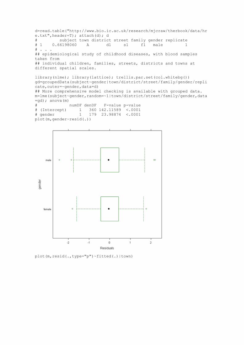
library(nlme); library(lattice); trellis.par.set(col.whitebg())
gd=groupedData(subject~gender|town/district/street/family/gender/repli
cate,outer=~gender,data=d)
## More comprehensive model checking is available with grouped data.
m=lme(subject~gender,random=~1|town/district/street/family/gender,data
=gd); anova(m)
# numDF denDF F-value p-value
# (Intercept) 1 360 142.11589 <.0001
# gender 1 179 23.98874 <.0001
plot(m,gender~resid(.))
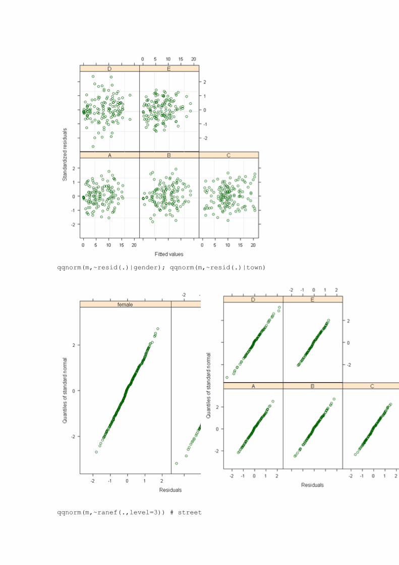
plot(m,resid(.,type="p")~fitted(.)|town)
Page 84
qqnorm(m,~resid(.)|gender); qqnorm(m,~resid(.)|town)
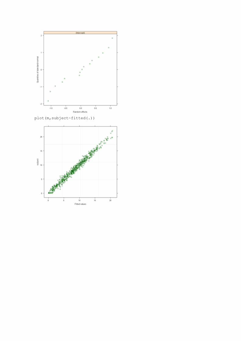
qqnorm(m,~ranef(.,level=3)) # street
Page 85
plot(m,subject~fitted(.))
Page 86
Learn R R is a free software environment for statistical computing and
graphics.
http://www.r-project.org/ Home | Getting Started | Schedule | References | FAQ | Discussion |
Tom's site | Other Courses For more information, please contact Paul Geissler
([email protected] ). Previous page
Topic 13 - Non-linear
Regression, Tree Methods, and Time Series Analysis, Crawley
(2007) Chapters 20, 21 and 22 Contents:
Non-linear Regression Tree Methods
Time Series Analysis The R code is available at
ftp://ftpext.usgs.gov/pub/cr/co/fort.collins/Geissler/LearnR/LearnR10-13.R
Chapter 20, Non-linear Regression Michael Crawley, 2007,The R Book, Chapter 20.
See the text for descriptions. You can copy and paste the statements below into the R Commander script window and execute them.
Anything after # on a line is a comment. I have added annotations as comments and shown the output as comments following each
command. Non-linear regression is used for relationships cannot be transformed
so that they are linear in the parameters. Many curved lines such as polynomials can be transformed to be
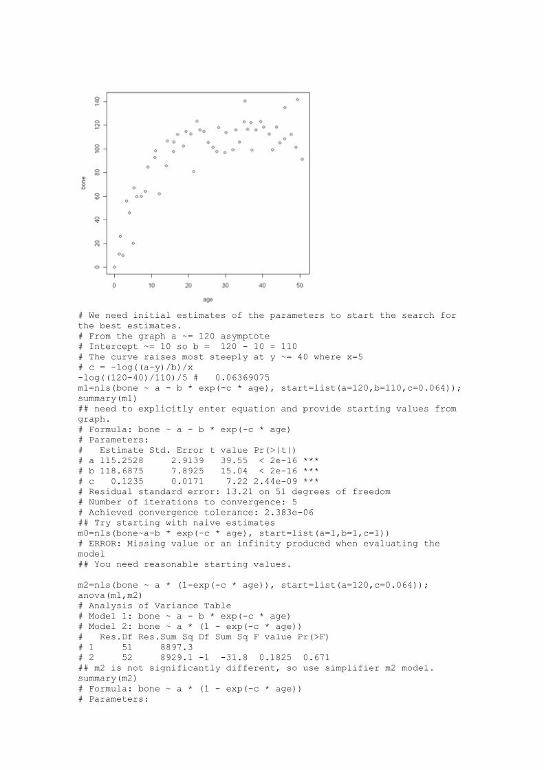
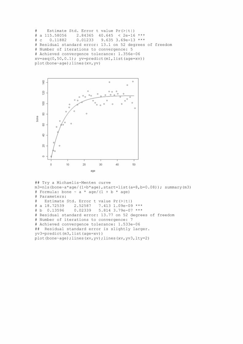
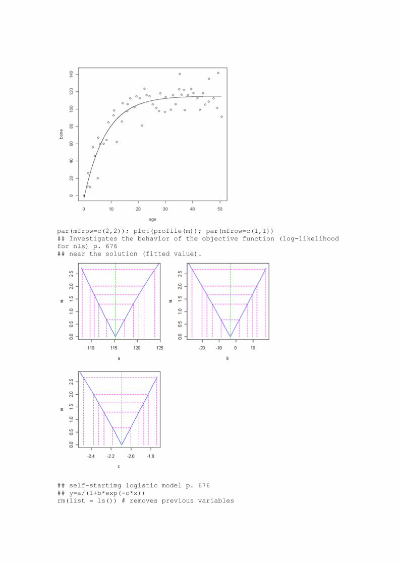
linear in the parameters and then fit by lm(). Example of jaw bone length (y) as a function of deer age (x).
Theory suggests the relationship y=a - b*exp(-cx) rm(list = ls()) # removes previous variables
d=read.table("http://www.bio.ic.ac.uk/research/mjcraw/therbook/data/ja
ws.txt",header=T); attach(d); d
# age bone # age deer with jaw bone length
# 1 0.000000 0.00000
# 2 5.112000 20.22000
# . . .
plot(age,bone)
Page 87
# We need initial estimates of the parameters to start the search for
the best estimates.
# From the graph a ~= 120 asymptote
# Intercept ~= 10 so b = 120 - 10 = 110
# The curve raises most steeply at y ~= 40 where x=5
# c = -log((a-y)/b)/x
-log((120-40)/110)/5 # 0.06369075
m1=nls(bone ~ a - b * exp(-c * age), start=list(a=120,b=110,c=0.064));
summary(m1)
## need to explicitly enter equation and provide starting values from
graph.
# Formula: bone ~ a - b * exp(-c * age)
# Parameters:
# Estimate Std. Error t value Pr(>|t|)
# a 115.2528 2.9139 39.55 < 2e-16 ***
# b 118.6875 7.8925 15.04 < 2e-16 ***
# c 0.1235 0.0171 7.22 2.44e-09 ***
# Residual standard error: 13.21 on 51 degrees of freedom
# Number of iterations to convergence: 5
# Achieved convergence tolerance: 2.383e-06
## Try starting with naive estimates
m0=nls(bone~a-b * exp(-c * age), start=list(a=1,b=1,c=1))
# ERROR: Missing value or an infinity produced when evaluating the
model
## You need reasonable starting values.
m2=nls(bone ~ a * (1-exp(-c * age)), start=list(a=120,c=0.064));
anova(m1,m2)
# Analysis of Variance Table
# Model 1: bone ~ a - b * exp(-c * age)
# Model 2: bone ~ a * (1 - exp(-c * age))
# Res.Df Res.Sum Sq Df Sum Sq F value Pr(>F)
# 1 51 8897.3
# 2 52 8929.1 -1 -31.8 0.1825 0.671
## m2 is not significantly different, so use simplifier m2 model.
summary(m2)
# Formula: bone ~ a * (1 - exp(-c * age))
# Parameters:
Page 88
# Estimate Std. Error t value Pr(>|t|)
# a 115.58056 2.84365 40.645 < 2e-16 ***
# c 0.11882 0.01233 9.635 3.69e-13 ***
# Residual standard error: 13.1 on 52 degrees of freedom
# Number of iterations to convergence: 5
# Achieved convergence tolerance: 1.356e-06
xv=seq(0,50,0.1); yv=predict(m1,list(age=xv))
plot(bone~age);lines(xv,yv)
## Try a Michaelis-Menten curve
m3=nls(bone~a*age/(1+b*age),start=list(a=8,b=0.08)); summary(m3)
# Formula: bone ~ a * age/(1 + b * age)
# Parameters:
# Estimate Std. Error t value Pr(>|t|)
# a 18.72539 2.52587 7.413 1.09e-09 ***
# b 0.13596 0.02339 5.814 3.79e-07 ***
# Residual standard error: 13.77 on 52 degrees of freedom
# Number of iterations to convergence: 7
# Achieved convergence tolerance: 1.533e-06
## Residual standard error is slightly larger.
yv3=predict(m3,list(age=xv))
plot(bone~age);lines(xv,yv);lines(xv,yv3,lty=2)
Page 89
#### generalized additive models ################################ page
665
## GAMs are useful when you don't know the functional form of the
relationship.
rm(list = ls()) # removes previous variables
d=read.table("http://www.bio.ic.ac.uk/research/mjcraw/therbook/data/hu
mp.txt",header=T); attach(d); d
# y x
# 1 3.741 0.907
# . . .
library(mgcv)
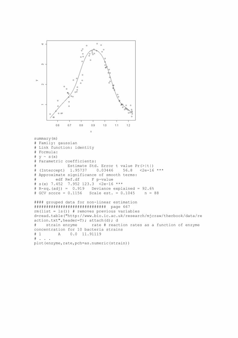
m=gam(y~s(x)) # s(x) is the smooth of x
xv=seq(min(x),max(x),0.001); yv=predict(m,list(x=xv))
plot(x,y); lines(xv,yv)
Page 90
summary(m)
# Family: gaussian
# Link function: identity
# Formula:
# y ~ s(x)
# Parametric coefficients:
# Estimate Std. Error t value Pr(>|t|)
# (Intercept) 1.95737 0.03446 56.8 <2e-16 ***
# Approximate significance of smooth terms:
# edf Ref.df F p-value
# s(x) 7.452 7.952 123.3 <2e-16 ***
# R-sq.(adj) = 0.919 Deviance explained = 92.6%
# GCV score = 0.1156 Scale est. = 0.1045 n = 88
#### grouped data for non-linear estimation
############################## page 667
rm(list = ls()) # removes previous variables
d=read.table("http://www.bio.ic.ac.uk/research/mjcraw/therbook/data/re
action.txt",header=T); attach(d); d
# strain enzyme rate # reaction rates as a function of enzyme
concentration for 10 bacteria strains
# 1 A 0.0 11.91119
# . . .
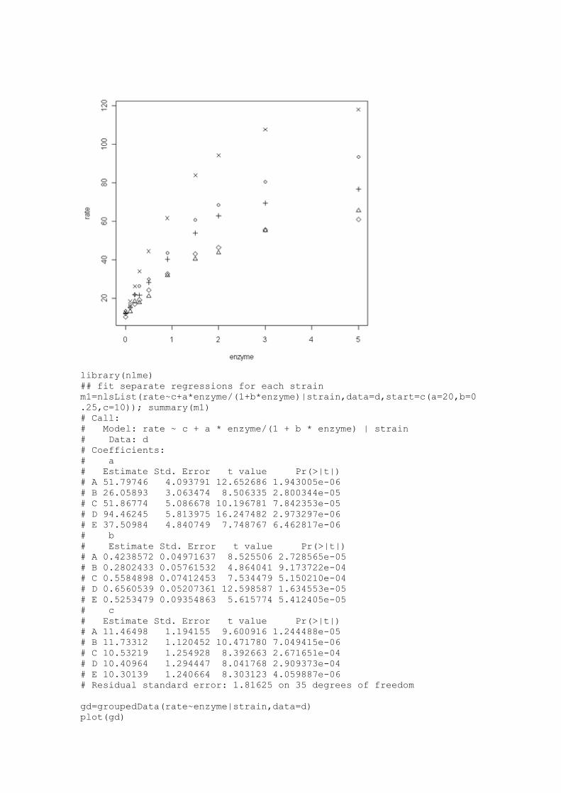
plot(enzyme,rate,pch=as.numeric(strain))
Page 91
library(nlme)
## fit separate regressions for each strain
m1=nlsList(rate~c+a*enzyme/(1+b*enzyme)|strain,data=d,start=c(a=20,b=0
.25,c=10)); summary(m1)
# Call:
# Model: rate ~ c + a * enzyme/(1 + b * enzyme) | strain
# Data: d
# Coefficients:
# a
# Estimate Std. Error t value Pr(>|t|)
# A 51.79746 4.093791 12.652686 1.943005e-06
# B 26.05893 3.063474 8.506335 2.800344e-05
# C 51.86774 5.086678 10.196781 7.842353e-05
# D 94.46245 5.813975 16.247482 2.973297e-06
# E 37.50984 4.840749 7.748767 6.462817e-06
# b
# Estimate Std. Error t value Pr(>|t|)
# A 0.4238572 0.04971637 8.525506 2.728565e-05
# B 0.2802433 0.05761532 4.864041 9.173722e-04
# C 0.5584898 0.07412453 7.534479 5.150210e-04
# D 0.6560539 0.05207361 12.598587 1.634553e-05
# E 0.5253479 0.09354863 5.615774 5.412405e-05
# c
# Estimate Std. Error t value Pr(>|t|)
# A 11.46498 1.194155 9.600916 1.244488e-05
# B 11.73312 1.120452 10.471780 7.049415e-06
# C 10.53219 1.254928 8.392663 2.671651e-04
# D 10.40964 1.294447 8.041768 2.909373e-04
# E 10.30139 1.240664 8.303123 4.059887e-06
# Residual standard error: 1.81625 on 35 degrees of freedom
gd=groupedData(rate~enzyme|strain,data=d)
plot(gd)
Page 92
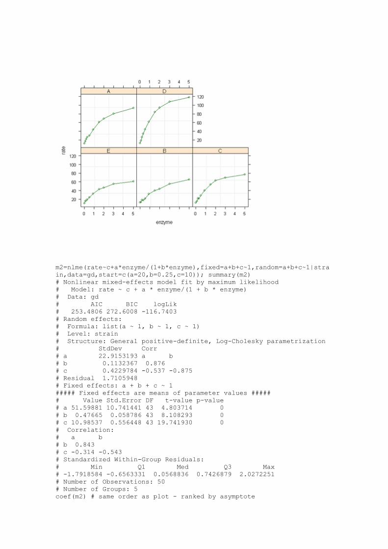
m2=nlme(rate~c+a*enzyme/(1+b*enzyme),fixed=a+b+c~1,random=a+b+c~1|stra
in,data=gd,start=c(a=20,b=0.25,c=10)); summary(m2)
# Nonlinear mixed-effects model fit by maximum likelihood
# Model: rate ~ c + a * enzyme/(1 + b * enzyme)
# Data: gd
# AIC BIC logLik
# 253.4806 272.6008 -116.7403
# Random effects:
# Formula: list(a ~ 1, b ~ 1, c ~ 1)
# Level: strain
# Structure: General positive-definite, Log-Cholesky parametrization
# StdDev Corr
# a 22.9153193 a b
# b 0.1132367 0.876
# c 0.4229784 -0.537 -0.875
# Residual 1.7105948
# Fixed effects: a + b + c ~ 1
##### Fixed effects are means of parameter values #####
# Value Std.Error DF t-value p-value
# a 51.59881 10.741441 43 4.803714 0
# b 0.47665 0.058786 43 8.108293 0
# c 10.98537 0.556448 43 19.741930 0
# Correlation:
# a b
# b 0.843
# c -0.314 -0.543
# Standardized Within-Group Residuals:
# Min Q1 Med Q3 Max
# -1.7918584 -0.6563331 0.0568836 0.7426879 2.0272251
# Number of Observations: 50
# Number of Groups: 5
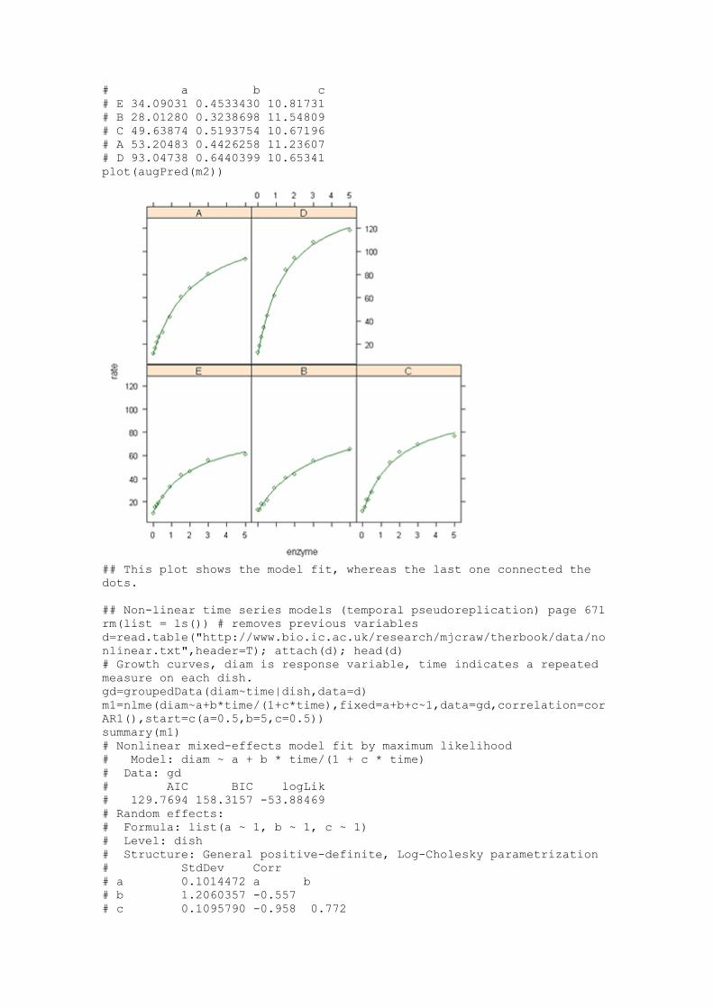
coef(m2) # same order as plot - ranked by asymptote
Page 93
# a b c
# E 34.09031 0.4533430 10.81731
# B 28.01280 0.3238698 11.54809
# C 49.63874 0.5193754 10.67196
# A 53.20483 0.4426258 11.23607
# D 93.04738 0.6440399 10.65341
plot(augPred(m2))
## This plot shows the model fit, whereas the last one connected the
dots.
## Non-linear time series models (temporal pseudoreplication) page 671
rm(list = ls()) # removes previous variables
d=read.table("http://www.bio.ic.ac.uk/research/mjcraw/therbook/data/no
nlinear.txt",header=T); attach(d); head(d)
# Growth curves, diam is response variable, time indicates a repeated
measure on each dish.
gd=groupedData(diam~time|dish,data=d)
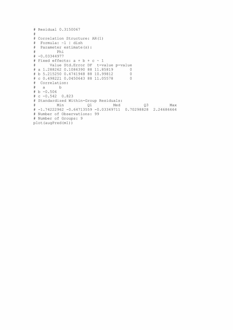
m1=nlme(diam~a+b*time/(1+c*time),fixed=a+b+c~1,data=gd,correlation=cor
AR1(),start=c(a=0.5,b=5,c=0.5))
summary(m1)
# Nonlinear mixed-effects model fit by maximum likelihood
# Model: diam ~ a + b * time/(1 + c * time)
# Data: gd
# AIC BIC logLik
# 129.7694 158.3157 -53.88469
# Random effects:
# Formula: list(a ~ 1, b ~ 1, c ~ 1)
# Level: dish
# Structure: General positive-definite, Log-Cholesky parametrization
# StdDev Corr
# a 0.1014472 a b
# b 1.2060357 -0.557
# c 0.1095790 -0.958 0.772
Page 94
# Residual 0.3150067
#
# Correlation Structure: AR(1)
# Formula: ~1 | dish
# Parameter estimate(s):
# Phi
# -0.03344977
# Fixed effects: a + b + c ~ 1
# Value Std.Error DF t-value p-value
# a 1.288262 0.1086390 88 11.85819 0
# b 5.215250 0.4741948 88 10.99812 0
# c 0.498221 0.0450643 88 11.05578 0
# Correlation:
# a b
# b -0.506
# c -0.542 0.823
# Standardized Within-Group Residuals:
# Min Q1 Med Q3 Max
# -1.74222962 -0.64713559 -0.03349711 0.70298828 2.24686664
# Number of Observations: 99
# Number of Groups: 9
plot(augPred(m1))
Page 95
range(time) # 0 10
xv=seq(0,10,0.1)
plot(time,diam,pch=as.numeric(dish),col=as.numeric(dish))
sapply(1:9,function(i)lines(xv,predict(m1,list(dish=i,time=xv)),lty=2)
)
Page 96
#### self-starting functions ################################ page
674
## Models will fail if the starting values are too far off.
## The most used self-starting functions are:
## SSasymp asymptotic regression model y=a-
b*exp(-c*x)
## SSasympOff asymptotic regression model with an offset y=a-
b*exp(-c*(x-d))
## SSasympOrig asymptotic regression model through the origin
y=a*(1-exp(-b*x))
## SSbiexp biexponential model
y=a*exp(b*x)-c*exp(-d*x)
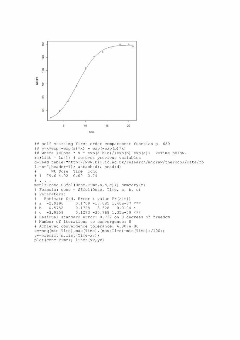
## SSfol first order compartment model
y=k*exp(-exp(a)*x)-exp(-exp(b)*x)
## SSfpl four-parameter logistic model
y=a+(b-a)/(1+exp(c-x)/d)
## SSgompertz Gompertz growth model
y=a*exp(b*exp(-c*x))
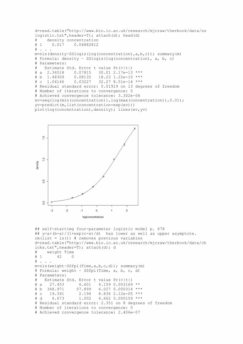
## SSlogis logistic model
y=a/(1+b*exp(-c*x))
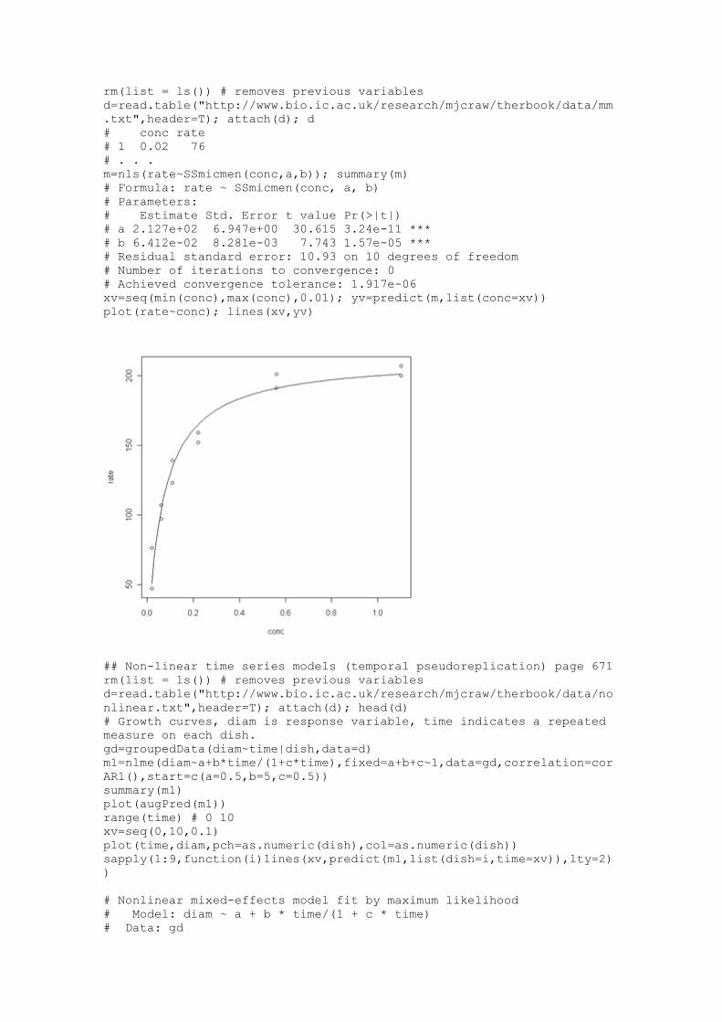
## SSmicmen Michaelis-Menten model
y=a*b/(b+x)
## SSweibull Weibull growth model y=a-
b*exp(c*x^d)
## self-startimg Michaelis-Menten model
## y=a*b/(b+x) a=asymptote, b=x for which y=a/2
Page 97
rm(list = ls()) # removes previous variables
d=read.table("http://www.bio.ic.ac.uk/research/mjcraw/therbook/data/mm
.txt",header=T); attach(d); d
# conc rate
# 1 0.02 76
# . . .
m=nls(rate~SSmicmen(conc,a,b)); summary(m)
# Formula: rate ~ SSmicmen(conc, a, b)
# Parameters:
# Estimate Std. Error t value Pr(>|t|)
# a 2.127e+02 6.947e+00 30.615 3.24e-11 ***
# b 6.412e-02 8.281e-03 7.743 1.57e-05 ***
# Residual standard error: 10.93 on 10 degrees of freedom
# Number of iterations to convergence: 0
# Achieved convergence tolerance: 1.917e-06
xv=seq(min(conc),max(conc),0.01); yv=predict(m,list(conc=xv))
plot(rate~conc); lines(xv,yv)
## Non-linear time series models (temporal pseudoreplication) page 671
rm(list = ls()) # removes previous variables
d=read.table("http://www.bio.ic.ac.uk/research/mjcraw/therbook/data/no
nlinear.txt",header=T); attach(d); head(d)
# Growth curves, diam is response variable, time indicates a repeated
measure on each dish.
gd=groupedData(diam~time|dish,data=d)
m1=nlme(diam~a+b*time/(1+c*time),fixed=a+b+c~1,data=gd,correlation=cor
AR1(),start=c(a=0.5,b=5,c=0.5))
summary(m1)
plot(augPred(m1))
range(time) # 0 10
xv=seq(0,10,0.1)
plot(time,diam,pch=as.numeric(dish),col=as.numeric(dish))
sapply(1:9,function(i)lines(xv,predict(m1,list(dish=i,time=xv)),lty=2)
)
# Nonlinear mixed-effects model fit by maximum likelihood
# Model: diam ~ a + b * time/(1 + c * time)
# Data: gd
Page 98
# AIC BIC logLik
# 129.7694 158.3157 -53.88469
# Random effects:
# Formula: list(a ~ 1, b ~ 1, c ~ 1)
# Level: dish
# Structure: General positive-definite, Log-Cholesky parametrization
# StdDev Corr
# a 0.1014472 a b
# b 1.2060357 -0.557
# c 0.1095790 -0.958 0.772
# Residual 0.3150067
# Correlation Structure: AR(1)
# Formula: ~1 | dish
# Parameter estimate(s):
# Phi
# -0.03344977
# Fixed effects: a + b + c ~ 1
# Value Std.Error DF t-value p-value
# a 1.288262 0.1086390 88 11.85819 0
# b 5.215250 0.4741948 88 10.99812 0
# c 0.498221 0.0450643 88 11.05578 0
# Correlation:
# a b
# b -0.506
# c -0.542 0.823
# Standardized Within-Group Residuals:
# Min Q1 Med Q3 Max
# -1.74222962 -0.64713559 -0.03349711 0.70298828 2.24686664
# Number of Observations: 99
# Number of Groups: 9
#### self-starting functions ################################ page
674
## Models will fail if the starting values are too far off.
## The most used self-starting functions are:
## SSasymp asymptotic regression model y=a-
b*exp(-c*x)
## SSasympOff asymptotic regression model with an offset y=a-
b*exp(-c*(x-d))
## SSasympOrig asymptotic regression model through the origin
y=a*(1-exp(-b*x))
## SSbiexp biexponential model
y=a*exp(b*x)-c*exp(-d*x)
## SSfol first order compartment model
y=k*exp(-exp(a)*x)-exp(-exp(b)*x)
## SSfpl four-parameter logistic model
y=a+(b-a)/(1+exp(c-x)/d)
## SSgompertz Gompertz growth model
y=a*exp(b*exp(-c*x))
## SSlogis logistic model
y=a/(1+b*exp(-c*x))
## SSmicmen Michaelis-Menten model
y=a*b/(b+x)
## SSweibull Weibull growth model y=a-
b*exp(c*x^d)
## self-startimg Michaelis-Menten model
## y=a*b/(b+x) a=asymptote, b=x for which y=a/2
rm(list = ls()) # removes previous variables
d=read.table("http://www.bio.ic.ac.uk/research/mjcraw/therbook/data/mm
.txt",header=T); attach(d); d
Page 99
# conc rate
# 1 0.02 76
# . . .
m=nls(rate~SSmicmen(conc,a,b)); summary(m)
# Formula: rate ~ SSmicmen(conc, a, b)
# Parameters:
# Estimate Std. Error t value Pr(>|t|)
# a 2.127e+02 6.947e+00 30.615 3.24e-11 ***
# b 6.412e-02 8.281e-03 7.743 1.57e-05 ***
# Residual standard error: 10.93 on 10 degrees of freedom
# Number of iterations to convergence: 0
# Achieved convergence tolerance: 1.917e-06
xv=seq(min(conc),max(conc),0.01); yv=predict(m,list(conc=xv))
plot(rate~conc); lines(xv,yv)
## self-startimg asymptotic exponential model
## y=a-b*exp(-c*x) a=asymptote, b=a-intercept, c=rate constant
rm(list = ls()) # removes previous variables
d=read.table("http://www.bio.ic.ac.uk/research/mjcraw/therbook/data/ja
ws.txt",header=T); attach(d); d
# age deer using length of jaw bones
# Example of jaw bone length (y) as a function of deer age (x).
# age bone
# 1 0.000000 0.00000
# 2 5.112000 20.22000
# . . .
m=nls(bone~SSasymp(age,a,b,c)); summary(m)
# Formula: bone ~ SSasymp(age, a, b, c)
# Parameters:
# Estimate Std. Error t value Pr(>|t|)
# a 115.2527 2.9139 39.553 <2e-16 ***
# b -3.4348 8.1961 -0.419 0.677
# c -2.0915 0.1385 -15.101 <2e-16 ***
# Residual standard error: 13.21 on 51 degrees of freedom
# Number of iterations to convergence: 0
# Achieved convergence tolerance: 2.438e-07
xv=seq(min(age),max(age),0.02); yv=predict(m,list(age=xv))
plot(bone~age); lines(xv,yv)
Page 100
par(mfrow=c(2,2)); plot(profile(m)); par(mfrow=c(1,1))
## Investigates the behavior of the objective function (log-likelihood
for nls) p. 676
## near the solution (fitted value).
## self-startimg logistic model p. 676
## y=a/(1+b*exp(-c*x))
rm(list = ls()) # removes previous variables
Page 101
d=read.table("http://www.bio.ic.ac.uk/research/mjcraw/therbook/data/ss
logistic.txt",header=T); attach(d); head(d)
# density concentration
# 1 0.017 0.04882812
# . . .
m=nls(density~SSlogis(log(concentration),a,b,c)); summary(m)
# Formula: density ~ SSlogis(log(concentration), a, b, c)
# Parameters:
# Estimate Std. Error t value Pr(>|t|)
# a 2.34518 0.07815 30.01 2.17e-13 ***
# b 1.48309 0.08135 18.23 1.22e-10 ***
# c 1.04146 0.03227 32.27 8.51e-14 ***
# Residual standard error: 0.01919 on 13 degrees of freedom
# Number of iterations to convergence: 0
# Achieved convergence tolerance: 3.302e-06
xv=seq(log(min(concentration)),log(max(concentration)),0.01);
yv=predict(m,list(concentration=exp(xv)))
plot(log(concentration),density); lines(xv,yv)
## self-startimg four-parameter logistic model p. 678
## y=a+(b-a)/(1+exp(c-x)/d) has lower as well as upper asymptote.
rm(list = ls()) # removes previous variables
d=read.table("http://www.bio.ic.ac.uk/research/mjcraw/therbook/data/ch
icks.txt",header=T); attach(d); d
# weight Time
# 1 42 0
# . . .
m=nls(weight~SSfpl(Time,a,b,c,d)); summary(m)
# Formula: weight ~ SSfpl(Time, a, b, c, d)
# Parameters:
# Estimate Std. Error t value Pr(>|t|)
# a 27.453 6.601 4.159 0.003169 **
# b 348.971 57.899 6.027 0.000314 ***
# c 19.391 2.194 8.836 2.12e-05 ***
# d 6.673 1.002 6.662 0.000159 ***
# Residual standard error: 2.351 on 8 degrees of freedom
# Number of iterations to convergence: 0
# Achieved convergence tolerance: 2.406e-07
Page 102
xv=seq(min(Time),max(Time),(max(Time)-min(Time))/100);
yv=predict(m,list(Time=xv))
plot(weight~Time); lines(xv,yv)
## self-startimg Weibull growth function p. 679
## y=a-b*exp(c*x^d)
rm(list = ls()) # removes previous variables
d=read.table("http://www.bio.ic.ac.uk/research/mjcraw/therbook/data/we
ibull.growth.txt",header=T); attach(d); head(d)
# weight time
# 1 49 2
# . . .
m=nls(weight~SSweibull(time,a,b,c,d)); summary(m)
# Formula: weight ~ SSweibull(time, a, b, c, d)
# Parameters:
# Estimate Std. Error t value Pr(>|t|)
# a 158.5012 1.1769 134.67 3.28e-13 ***
# b 110.9971 2.6330 42.16 1.10e-09 ***
# c -5.9934 0.3733 -16.05 8.83e-07 ***
# d 2.6461 0.1613 16.41 7.62e-07 ***
# Residual standard error: 2.061 on 7 degrees of freedom
# Number of iterations to convergence: 0
# Achieved convergence tolerance: 5.702e-06
xv=seq(min(time),max(time),(max(time)-min(time))/100);
yv=predict(m,list(time=xv))
plot(weight~time); lines(xv,yv)
Page 103
## self-startimg first-order compartment function p. 680
## y=k*exp(-exp(a)*x) - exp(-exp(b)*x)
## where k=Dose * x * exp(a+b+c)/(exp(b)-exp(a)) x=Time below.
rm(list = ls()) # removes previous variables
d=read.table("http://www.bio.ic.ac.uk/research/mjcraw/therbook/data/fo
l.txt",header=T); attach(d); head(d)
# Wt Dose Time conc
# 1 79.6 4.02 0.00 0.74
# . . .
m=nls(conc~SSfol(Dose,Time,a,b,c)); summary(m)
# Formula: conc ~ SSfol(Dose, Time, a, b, c)
# Parameters:
# Estimate Std. Error t value Pr(>|t|)
# a -2.9196 0.1709 -17.085 1.40e-07 ***
# b 0.5752 0.1728 3.328 0.0104 *
# c -3.9159 0.1273 -30.768 1.35e-09 ***
# Residual standard error: 0.732 on 8 degrees of freedom
# Number of iterations to convergence: 8
# Achieved convergence tolerance: 4.907e-06
xv=seq(min(Time),max(Time),(max(Time)-min(Time))/100);
yv=predict(m,list(Time=xv))
plot(conc~Time); lines(xv,yv)
Page 104
Chapter 21, Tree Models Tree models are computationally intensive methods that are used in situations where there are many explanatory variables, and we would
like guidance about which of them to include in the model. Tree models are particularly good at tasks that might be regarded as
appropriate for multivariate statistics, such as classification problems.
Their advantages are that they: • are very simple
• are excellent for initial data inspection • give a very clear picture of the structure of the data
• provide a highly intuitive insight into the interactions
The model is fit using binary recursive partitioning, where the data are successively split so that at any node, the split that maximally
distinguishes the response variable is selected. Each explanatory variable is assessed turn and the variable explaining the greatest
amount of deviance in the response variable is selected. Deviance is defined as D=Σ(yi-u|i|)
2 where u|i| is the mean of all the response
values assigned to node i and the sum of squares add over all nodes. The value of any split is defined as the reduction in this residual sum
of squares. The procedure is:
• Select a threshold value of an explanatory variable. • Calculate the mean value of the response variable above and below
this threshold value of the explanatory variable. • Use these two means u|i| to calculate the deviance D.
• Loop through all possible values of the threshold for all the explanatory variable.
• Determine which value of the threshold gives the lowest deviance.
Page 105
• Split the data into high and low subsets on the basis of the
threshold for this response variable. • Repeat the procedure on each subset of the data on either side of
the threshold.
• Keep going until no further reduction id deviance is obtained, or there are too few data points to merit further subdivision.
If the explanatory variable are categorical, it is a classification tree.
If the explanatory variable are continuous, it is a regression tree. regression trees library(tree)
rm(list = ls()) # removes previous variables
d=read.table("http://www.bio.ic.ac.uk/research/mjcraw/therbook/data/Po
llute.txt",header=T); attach(d); head(d)
# Pollution Temp Industry Population Wind Rain Wet.days
# 1 24 61.5 368 497 9.1 48.34 115
# . . .
m1=tree(Pollution~.,d); plot(m1); text(m1)
m1
# node), split, n, deviance, yval
# * denotes terminal node
# 1) root 41 22040 30.05
# 2) Industry < 748 36 11260 24.92
# 4) Population < 190 7 4096 43.43 *
# 5) Population > 190 29 4187 20.45
# 10) Wet.days < 108 11 96 12.00 *
# 11) Wet.days > 108 18 2826 25.61
# 22) Temp < 59.35 13 1895 29.69
# 44) Wind < 9.65 8 1213 33.88 *
# 45) Wind > 9.65 5 318 23.00 *
Page 106
# 23) Temp > 59.35 5 152 15.00 *
# 3) Industry > 748 5 3002 67.00 *
## in the line "2) Industry < 748 36 11260 24.92"
## "2)" labels the node
## "Industry < 748" is the split criterion
## "36" is the number of cases going into the split
## "11260" is the deviance at the node
## "24.92" is the mean of the response variable at the node.
## * indicates a terminal node (estimate)
d1=data.frame(d,node=as.numeric(m1$where),predicted=predict(m1));
attach(d1)
d1[order(node),]
## Nodes are numbered differently than above.
## Node 3: Industry < 748 and Population < 190
# Pollution Temp Industry Population Wind Rain Wet.days node
predicted
# 4 28 51.0 137 176 8.7 15.17 89 3
43.42857
# 6 46 47.6 44 116 8.8 33.36 135 3
43.42857
# 18 13 61.0 91 132 8.2 48.52 100 3
43.42857
# 19 31 55.2 35 71 6.6 40.75 148 3
43.42857
# 23 56 49.1 412 158 9.0 43.37 127 3
43.42857
# 27 36 54.0 80 80 9.0 40.25 114 3
43.42857
# 41 94 50.0 343 179 10.6 42.75 125 3
43.42857
## Node 5: Industry < 748 and Population > 190 and Wet.days < 108
# Pollution Temp Industry Population Wind Rain Wet.days node
predicted
# 7 9 66.2 641 844 10.9 35.94 78 5
12.00000
# 13 14 51.5 181 347 10.9 30.18 98 5
12.00000
# 15 17 51.9 454 515 9.0 12.95 86 5
12.00000
# 20 12 56.7 453 716 8.7 20.66 67 5
12.00000
# 21 10 70.3 213 582 6.0 7.05 36 5
12.00000
# 24 10 68.9 721 1233 10.8 48.19 103 5
12.00000
# 26 8 56.6 125 277 12.7 30.58 82 5
12.00000
# 36 10 61.6 337 624 9.2 49.10 105 5
12.00000
# 38 14 54.5 381 507 10.0 37.00 99 5
12.00000
# 39 17 49.0 104 201 11.2 30.85 103 5
12.00000
# 40 11 56.8 46 244 8.9 7.77 58 5
12.00000
## Node 8: Industry < 748 and Population > 190 and Wet.days > 108
## and Temp < 59.35 and Wind < 9.65
# Pollution Temp Industry Population Wind Rain Wet.days node
predicted
Page 107
# 2 30 55.6 291 593 8.3 43.11 123 8
33.87500
# 9 26 57.8 197 299 7.6 42.59 115 8
33.87500
# 10 61 50.4 347 520 9.4 36.22 147 8
33.87500
# 11 29 57.3 434 757 9.3 38.98 111 8
33.87500
# 16 23 54.0 462 453 7.1 39.04 132 8
33.87500
# 17 47 55.0 625 905 9.6 41.31 111 8
33.87500
# 29 29 51.1 379 531 9.4 38.79 164 8
33.87500
# 34 26 51.5 266 540 8.6 37.01 134 8
33.87500
## Node 9: Industry < 748 and Population > 190 and Wet.days > 108
## and Temp < 59.35 and Wind > 9.65
# Pollution Temp Industry Population Wind Rain Wet.days node
predicted
# 12 28 52.3 361 746 9.7 38.74 121 9
23.00000
# 28 16 45.7 569 717 11.8 29.07 123 9
23.00000
# 30 29 43.5 669 744 10.6 25.94 137 9
23.00000
# 35 31 59.3 96 308 10.6 44.68 116 9
23.00000
# 37 11 47.1 391 463 12.4 36.11 166 9
23.00000
## Node 10: Industry < 748 and Population > 190 and Wet.days > 108
## and Temp > 59.35
# Pollution Temp Industry Population Wind Rain Wet.days node
predicted
# 1 24 61.5 368 497 9.1 48.34 115 10
15.00000
# 5 14 68.4 136 529 8.8 54.47 116 10
15.00000
# 14 18 59.4 275 448 7.9 46.00 119 10
15.00000
# 32 9 68.3 204 361 8.4 56.77 113 10
15.00000
# 33 10 75.5 207 335 9.0 59.80 128 10
15.00000
## Node 11: Industry > 748
# Pollution Temp Industry Population Wind Rain Wet.days node
predicted
# 3 56 55.9 775 622 9.5 35.89 105 11
67.00000
# 8 35 49.9 1064 1513 10.1 30.96 129 11
67.00000
# 22 110 50.6 3344 3369 10.4 34.44 122 11
67.00000
# 25 69 54.6 1692 1950 9.6 39.93 115 11
67.00000
# 31 65 49.7 1007 751 10.9 34.99 155 11
67.00000
plot(node,Pollution)
Page 108
#### tree models as regressions
########################################## page 689
d=read.table("http://www.bio.ic.ac.uk/research/mjcraw/therbook/data/ca
r.test.frame.txt",header=T); attach(d); head(d)
# Price Country Reliability Mileage Type Weight Disp. HP
# 1 8895 USA 4 33 Small 2560 97 113
# . . .
plot(Weight,Mileage)
m2=tree(Mileage~Weight); plot(m2); text(m2)
Page 109
xv=seq(min(Weight),max(Weight),10); yv=predict(m2,list(Weight=xv))
plot(Weight,Mileage); lines(xv,yv)
#### model simplification ############################### page 690
## Simplification is a comprise between fit and explanatory power,
## because a model with perfect fit would have as many parameters and
data points.
## prune.tree() returns a nested sequence of sub-trees by recursively
'snipping' off the least
Page 110
## important splits, based on a cost-complexity measure.
pt=prune.tree(m1); pt # pollution example
# $size # number of terminal nodes
# [1] 6 5 4 3 2 1
# $dev # total deviance of each subtree
# [1] 8876.589 9240.484 10019.992 11284.887 14262.750 22037.902
# $k # cpst-complexity pruning parameter.
# [1] -Inf 363.8942 779.5085 1264.8946 2977.8633 7775.1524
# $method
# [1] "deviance"
# attr(,"class")
# [1] "prune" "tree.sequence"
m3=prune.tree(m1,best=4); m3 # best tree with 4 terminal nodes
# node), split, n, deviance, yval
# * denotes terminal node
# 1) root 41 22040 30.05
# 2) Industry < 748 36 11260 24.92
# 4) Population < 190 7 4096 43.43 *
# 5) Population > 190 29 4187 20.45
# 10) Wet.days < 108 11 96 12.00 *
# 11) Wet.days > 108 18 2826 25.61 *
# 3) Industry > 748 5 3002 67.00 *
plot(m3); text(m3)
#### classification trees with categorical explanatory variables
########### page 693
## Tree models are very useful for developing efficient and effective
taxonomic keys.
## First split where it explains the most variability.
rm(list = ls()) # removes previous variables
d=read.table("http://www.bio.ic.ac.uk/research/mjcraw/therbook/data/ep
ilobium.txt",header=T); attach(d); d
# species stigma stem.hairs glandular.hairs seeds pappilose
stolons petals base
# 1 hirsutum lobed spreading absent none uniform
absent <9mm rounded
Page 111
# 2 parviflorum lobed spreading absent none uniform
absent >10mm rounded
# 3 montanum lobed spreading present none uniform
absent >10mm rounded
# 4 lanceolatum lobed spreading present none uniform
absent >10mm cuneate
# 5 tetragonum clavate appressed present none uniform
absent >10mm rounded
# 6 obscurum clavate appressed present none uniform
stolons >10mm rounded
# 7 roseum clavate spreading present none uniform
absent >10mm cuneate
# 8 palustre clavate spreading present appendage uniform
absent >10mm rounded
# 9 ciliatum clavate spreading present appendage ridged
absent >10mm rounded
m=tree(species~.,d);m # only one node because only 1 entry for each
species
# node), split, n, deviance, yval, (yprob)
# * denotes terminal node
# 1) root 9 39.55 ciliatum ( 0.1111 0.1111 0.1111 0.1111 0.1111 0.1111
0.1111 0.1111 0.1111 ) *
m=tree(species~.,d,minsize=2,mindev=1e-6);m
# node), split, n, deviance, yval, (yprob)
# * denotes terminal node
# 1) root 9 39.550 ciliatum ( 0.1111 0.1111 0.1111 0.1111 0.1111
0.1111 0.1111 0.1111 0.1111 )
# 2) stigma: clavate 5 16.090 ciliatum ( 0.2000 0.0000 0.0000
0.0000 0.2000 0.2000 0.0000 0.2000 0.2000 )
# 4) stem.hairs: appressed 2 2.773 obscurum ( 0.0000 0.0000
0.0000 0.0000 0.5000 0.0000 0.0000 0.0000 0.5000 )
# 8) stolons: absent 1 0.000 tetragonum ( 0.0000 0.0000 0.0000
0.0000 0.0000 0.0000 0.0000 0.0000 1.0000 ) *
# 9) stolons: stolons 1 0.000 obscurum ( 0.0000 0.0000 0.0000
0.0000 1.0000 0.0000 0.0000 0.0000 0.0000 ) *
# 5) stem.hairs: spreading 3 6.592 ciliatum ( 0.3333 0.0000
0.0000 0.0000 0.0000 0.3333 0.0000 0.3333 0.0000 )
# 10) seeds: appendage 2 2.773 ciliatum ( 0.5000 0.0000 0.0000
0.0000 0.0000 0.5000 0.0000 0.0000 0.0000 )
# 20) pappilose: ridged 1 0.000 ciliatum ( 1.0000 0.0000
0.0000 0.0000 0.0000 0.0000 0.0000 0.0000 0.0000 ) *
# 21) pappilose: uniform 1 0.000 palustre ( 0.0000 0.0000
0.0000 0.0000 0.0000 1.0000 0.0000 0.0000 0.0000 ) *
# 11) seeds: none 1 0.000 roseum ( 0.0000 0.0000 0.0000 0.0000
0.0000 0.0000 0.0000 1.0000 0.0000 ) *
# 3) stigma: lobed 4 11.090 hirsutum ( 0.0000 0.2500 0.2500 0.2500
0.0000 0.0000 0.2500 0.0000 0.0000 )
# 6) glandular.hairs: absent 2 2.773 hirsutum ( 0.0000 0.5000
0.0000 0.0000 0.0000 0.0000 0.5000 0.0000 0.0000 )
# 12) petals: <0mm 1 0.000 parviflorum ( 0.0000 0.0000 0.0000
0.0000 0.0000 0.0000 1.0000 0.0000 0.0000 ) *
# 13) petals: >9mm 1 0.000 hirsutum ( 0.0000 1.0000 0.0000
0.0000 0.0000 0.0000 0.0000 0.0000 0.0000 ) *
# 7) glandular.hairs: present 2 2.773 lanceolatum ( 0.0000
0.0000 0.5000 0.5000 0.0000 0.0000 0.0000 0.0000 0.0000 )
# 14) base: cuneate 1 0.000 lanceolatum ( 0.0000 0.0000 1.0000
0.0000 0.0000 0.0000 0.0000 0.0000 0.0000 ) *
# 15) base: rounded 1 0.000 montanum ( 0.0000 0.0000 0.0000
1.0000 0.0000 0.0000 0.0000 0.0000 0.0000 ) *
plot(m); text(m)
Page 112
#### classification trees for replicated data ######################
page 695
rm(list = ls()) # removes previous variables
d=read.table("http://www.bio.ic.ac.uk/research/mjcraw/therbook/data/ta
xonomy.txt",header=T); attach(d); head(d)
## Construct the key for the four taxa with the smallest error rate.
# Taxon Petals Internode Sepal Bract Petiole Leaf
Fruit
# 1 I 5.621498 29.48060 2.462107 18.20341 11.279097 1.128033
7.876151
# . . .
m1=tree(Taxon~.,d); m1
# node), split, n, deviance, yval, (yprob)
# * denotes terminal node
# 1) root 120 332.70 I ( 0.2500 0.2500 0.2500 0.2500 )
# 2) Sepal < 3.53232 90 197.80 I ( 0.3333 0.3333 0.3333 0.0000 )
# 4) Leaf < 2.00426 60 83.18 I ( 0.5000 0.5000 0.0000 0.0000 )
# 8) Petiole < 9.91246 30 0.00 II ( 0.0000 1.0000 0.0000
0.0000 ) *
# 9) Petiole > 9.91246 30 0.00 I ( 1.0000 0.0000 0.0000 0.0000
) *
# 5) Leaf > 2.00426 30 0.00 III ( 0.0000 0.0000 1.0000 0.0000 )
*
# 3) Sepal > 3.53232 30 0.00 IV ( 0.0000 0.0000 0.0000 1.0000 ) *
plot(m1); text(m1)
Page 113
summary(m1)
# Classification tree:
# tree(formula = Taxon ~ ., data = d)
# Variables actually used in tree construction:
# [1] "Sepal" "Leaf" "Petiole"
# Number of terminal nodes: 4
# Residual mean deviance: 0 = 0 / 116
# Misclassification error rate: 0 = 0 / 120 # impressive
Page 114
Chapter 22, Time Series Analysis Time series data are vectors of numbers, typically regularly spaced in time. rm(list = ls()) # removes previous variables
d=read.table("http://www.bio.ic.ac.uk/research/mjcraw/therbook/data/bl
owfly.txt",header=T); attach(d); head(d)
# flies # A. J. Nicholson reared blowfly larvae in a laboratory
# 1 948 # and kept the experiment running for almost seven years.
# 2 942
# . . .
# 361 6803
# 362 \032
## The last point seems to be bad, so I will remove it.
d=d[1:361,]
flies=ts(d); plot(flies) # time series object
#
## You can see the pattern better by changes the aspect ratio.
library(lattice)
xyplot(flies~1:length(flies), type="l" ,aspect=0.3, xlab="")
#
Page 115
## The process seems to have changed around week 200.
n=length(flies); n
par(mfrow=c(2,2))
## Plot lags, such as flies[1] vs flies[2], and flies[1] vs flies[3],
etc.
## Need to make the vectors the same length, so they match.
sapply(1:4, function(x) plot(as.numeric(flies[-c(n-
x+1:n)]),as.numeric(flies[-c(1:x)])) )
par(mfrow=c(1,1))
#
## The correlation drops off quickly with increasing lags.
## Autocorrelation is the correlation between successive observations
over time.
## Partial autocorrelations adjust for the effects of correlations
with fewer lags.
par(mfrow=c(1,2))
acf(flies,main="autocorrelation")
acf(flies, type="p",main="partial autocorrelation")
par(mfrow=c(1,1))
Page 116
#
## At lag 0, autocorrelation with itself is 1.
## Partial autocorrelations starts with lag 1, which is the same as
the autocorrelation.
## The autocorrelation drops off with time, but becomes negative with
the next down slope of the cycle.
## The negative partial autocorrelation at lags 2 and 3 reflects the
length of the
## larval (1 week) and pupal (2 weeks) periods.
## Cycles are caused by over compensating density dependence,
resulting form larval competition for food.
## It looks like the process is different after week 200.
period=numeric(n); period[1:200]=0; period[201:n]=1; weeks=1:n
m1=lm(flies~weeks*period); anova(m1)
# Analysis of Variance Table
# Response: flies
# Df Sum Sq Mean Sq F value Pr(>F)
# weeks 1 8091 8091 0.8299 0.3629
# period 1 424 424 0.0435 0.8349
# weeks:period 1 258019 258019 26.4662 4.434e-07 ***
# Residuals 357 3480395 9749
m2=lm(flies~weeks+period); anova(m1,m2)
# Analysis of Variance Table
# Model 1: flies ~ weeks * period
# Model 2: flies ~ weeks + period
# Res.Df RSS Df Sum of Sq F Pr(>F)
# 1 357 3480395
# 2 358 3738414 -1 -258019 26.466 4.434e-07 ***
## Both the intercept and slope changes after week 200,
##so we should analyze these periods separately.
flies1=flies[1:200]; weeks1=1:200; flies2=flies[201:n];
weeks2=1:length(flies2)
Page 117
m1=lm(flies1~weeks1);summary(m1)
# Coefficients:
# Estimate Std. Error t value Pr(>|t|)
# (Intercept) 204.4682 15.3166 13.349 <2e-16 ***
# weeks1 -0.3012 0.1322 -2.279 0.0237 *
m2=lm(flies2~weeks2);summary(m2)
# Coefficients:
# Estimate Std. Error t value Pr(>|t|)
# (Intercept) 119.6196 13.6147 8.786 2.37e-15 ***
# weeks2 0.7613 0.1458 5.222 5.47e-07 ***
## Decrease in period 1, but an increase in period 2.
## Tests do not consider autocorrelations (spatial pseudoreplication).
dt1=flies1-predict(m1); dt2=flies2-predict(m2) # detrended
par(mfrow=c(1,3))
ts.plot(dt1)
acf(dt1, main="autocorrelation")
acf(dt1, type="p", main="partial autocorrelation")
#
ts.plot(dt2)
acf(dt2, main="autocorrelation")
acf(dt2, type="p", main="partial autocorrelation")
par(mfrow=c(1,1))
#
Page 118
#### moving average ##############################################
page 708
rm(list = ls()) # removes previous variables
d=read.table("http://www.bio.ic.ac.uk/research/mjcraw/therbook/data/te
mp.txt",header=T); attach(d); head(d)
# temps
# 1 3.170968
# . . .
## A three point moving average removes much of the local noise.
## yi = (xi-1 + xi + xi+1)/3
ma=function(x,d) {
d=as.integer(d/2); n=length(x); y=numeric(n); y[1:d]=NA; y[(n-
d+1):n]=NA
for (i in (d+1):(n-d)) y[i]=mean(x[(i-d):(i+d)])
y
}
par(mfrow=c(3,1))
plot(temps, main="points"); lines(temps);
mavg=ma(temps,3); plot(temps,main="moving average 3");
lines(ma(temps,3))
mavg=ma(temps,7); plot(temps,main="moving average 7");
lines(ma(temps,7))
par(mfrow=c(1,1))
Page 119
#
## Note the seasonal pattern.
#### seasonal data ###############################################
page 708
rm(list = ls()) # removes previous variables
d=read.table("http://www.bio.ic.ac.uk/research/mjcraw/therbook/data/Si
lwoodWeather.txt",header=T); attach(d); head(d)
# upper lower rain month yr # daily weather from Silwood Park,
England 1987-2005
# 1 10.8 6.5 12.2 1 1987
# 2 10.5 4.5 1.3 1 1987
# . . .
plot(upper,type="l")
Page 120
#
n=length(upper); n; yrLen=n/19; yrLen # n=6940, yr=365.2632 days
t=(1:n)/yrLen; head(t) # time in years
m=lm(upper~sin(t*2*pi)+cos(t*2*pi)); summary(m)
# Coefficients:
# Estimate Std. Error t value Pr(>|t|)
# (Intercept) 14.95647 0.04088 365.86 <2e-16 ***
# sin(t * 2 * pi) -2.53888 0.05781 -43.91 <2e-16 ***
# cos(t * 2 * pi) -7.24015 0.05781 -125.23 <2e-16 ***
plot(t,upper,pch="."); lines(t,predict(m))
Page 121
#
plot(m$resid,pch=".")
Page 122
#
## some periodicity, but no obvious trend
par(mfrow=c(1,2)); acf(m$resid); acf(m$resid,type="p");
par(mfrow=c(1,1));
Page 123
#
## strong autocorrelation, which drop off quickly
## Only the partial autocorrelation at lag 1 is large,
## suggesting an autoregressive model with lag 1, AR(1).
#### pattern in monthly means ############################### page
713
moMeans=tapply(upper,list(month,yr),mean) # monthly means
temp=ts(as.vector(moMeans))
par(mfrow=c(1,2)); plot(temp); acf(temp); par(mfrow=c(1,1))
Page 124
#
## cycle with period of 12 months
yrMeans=tapply(upper,yr,mean) # monthly means
ytemp=ts(as.vector(yrMeans))
par(mfrow=c(1,2)); plot(ytemp); acf(ytemp); par(mfrow=c(1,1))
#
## No evidence for autocorrelation among years.
#### built-in time series functions ######################### page
714
high=ts(upper,start=c(1987,1),frequency=365); plot(high) # time series
object
Page 125
#
## decomposition
up=stl(high,"periodic"); plot(up) # Seasonal Decomposition
Page 126
#
## testing for a trend in time series
tapply(upper, factor(yr>1996), mean)
# FALSE TRUE # mean after 1966 is greater
# 14.62056 15.32978
yr=factor(yr); n=length(upper); ix=1:n; yrLen=n/19; t=(1:n)/yrLen #
time in years
library(lme4)
m1=lmer(upper~ix+sin(t*2*pi)+cos(t*2*pi) + (1|factor(yr)), REML=F)
m2=lmer(upper~sin(t*2*pi)+cos(t*2*pi) + (1|factor(yr)), REML=F) #
remove ix index
anova(m1,m2)
# Models:
# m2: upper ~ sin(t * 2 * pi) + cos(t * 2 * pi) + (1 | yr)
# m1: upper ~ ix + sin(t * 2 * pi) + cos(t * 2 * pi) + (1 | yr)
# Df AIC BIC logLik Chisq Chi Df Pr(>Chisq)
# m2 5 36452 36486 -18221
# m1 6 36458 36499 -18223 0 1 1
Page 127
## m2, without ix, is preferred. No suggestion of global warming.
m3=lm(yrMeans~I(1:length(yrMeans))); summary(m3)
## Analyzing yearly means removes the spatial pseudoreplication,
because they are uncorrelated.
# Coefficients:
# Estimate Std. Error t value Pr(>|t|)
# (Intercept) 14.27105 0.32220 44.293 <2e-16 ***
# I(1:length(yrMeans)) 0.06858 0.02826 2.427 0.0266 *
## Significantly increasing trend.
m4=lm(yrMeans[-1]~I(1:(length(yrMeans)-1))); summary(m4)
# Coefficients:
# Estimate Std. Error t value Pr(>|t|)
# (Intercept) 14.59826 0.30901 47.243 <2e-16 ***
# I(1:(length(yrMeans) - 1)) 0.04761 0.02855 1.668 0.115
## Not significant if drop first year.
#### spectral analysis ##################################### Page 717
## Spectral analysis is an alternative approach that is based on the
analysis of
## frequencies rather than the fluctuations of numbers.
rm(list = ls()) # removes previous variables
d=read.table("http://www.bio.ic.ac.uk/research/mjcraw/therbook/data/ly
nx.txt",header=T); attach(d); head(d)
# Lynx # annual number of lynx pelts bought by Hudson's Bay
Company
# 1 269
# . . .
plot.ts(Lynx)
#
spectrum(lynx)
Page 128
#
## The graph is interpreted as showing strong cycles with a frequency
of about 0.1.
## The vertical blue bar shows the 95% confidence interval.
## A frequency of 0.1 indicates a period of 1/0.1 = 10 years.
#### multiple time series ########################################
Page 718
rm(list = ls()) # removes previous variables
d=read.table("http://www.bio.ic.ac.uk/research/mjcraw/therbook/data/tw
oseries.txt",header=T); attach(d); head(d)
# x y
# 1 101 121
# . . .
plot.ts(cbind(x,y))
Page 129
#
par(mfrow=c(1,2)); acf(x,type="p"); acf(y,type="p");
par(mfrow=c(1,1));
#
## The evidence for periodicity is stronger in x than in y.
## The partial autocorrelation for x is significant at a lag of 2.
Page 130
acf(cbind(x,y))
#
## x & y is the cross correlation of the two time series
## The lag is reversed for y & x.
acf(cbind(x,y),type="p")
Page 131
#
## Partial autocorrelations control for both x and y.
plot(diff(x),diff(y))
#
## Plotting the differences shows a negative correlation, with two
outliers.
#### simulated time series ################################## Page
722
## Shows how a first-order autoregressive process [AR(1)] appears in
the plots.
Page 132
rm(list = ls()) # removes previous variables
n=250; e=rnorm(n,0,2)# error term
y=e # no autocorrelation.
par(mfrow=c(1,3)); plot.ts(y); acf(y); acf(y,type="p")
#
a=-0.5; y[1]=e[1]
for (i in 2:n) y[i]=a*y[i-1]+e[i]
par(mfrow=c(1,3)); plot.ts(y); acf(y); acf(y,type="p")
#
a=0.5; y[1]=e[1]
for (i in 2:n) y[i]=a*y[i-1]+e[i]
par(mfrow=c(1,3)); plot.ts(y); acf(y); acf(y,type="p")
Page 133
#
a=1; y[1]=e[1] # random walk
for (i in 2:n) y[i]=a*y[i-1]+e[i]
par(mfrow=c(1,3)); plot.ts(y); acf(y); acf(y,type="p")
#
par(mfrow=c(1,1))
#### time series models ############################ Page 726
• Moving average (AV)
• Autoregressive (AR)
• Autoregressive moving average (ARMA)
rm(list = ls()) # removes previous variables
d=read.table("http://www.bio.ic.ac.uk/research/mjcraw/therbook/data/ly
nx.txt",header=T); attach(d); head(d)
# Lynx # annual number of lynx pelts bought by Hudson's Bay
Company
# 1 269
# . . .
par(mfrow=c(1,2)); acf(Lynx); acf(Lynx,type="p"); par(mfrow=c(1,1))
Page 134
#
## Crawley comments that "the population is very clearly cyclic, with
a period
## of 10 years. The dynamics appear to be driven by strong, negative
density dependence
##(a partial autocorrelation of =0.588) at lag 2. There are other
significant partials
## at lags 1 and 8 (positive) and lag 4 (negative). Of course you
cannot infer the
## mechanism by observing the dynamics, but the lags associated with
significant negative
## and positive feedbacks are extremely interesting and highly
suggestive.
## The main prey species of the lynx is the snowshoe hare and the
negative feedback at
## lag 2 may reflect the timescale of this predator-prey interaction.
The hares are
## known to cause medium-term induced reductions in the quality of
their food plants as
## a result of heavy browsing pressure when the hares [are] at high
density, and this
## could map through to lynx populations with lag 4."
## arima (autoregressive moving average models) order=c(p,d,q) where
## p = autoregressive order
## d = degree of differencing
## q = moving average order
m100=arima(Lynx,order=c(1,0,0))
m200=arima(Lynx,order=c(2,0,0))
m300=arima(Lynx,order=c(3,0,0))
m400=arima(Lynx,order=c(4,0,0))
m500=arima(Lynx,order=c(5,0,0))
m600=arima(Lynx,order=c(6,0,0))
m001=arima(Lynx,order=c(0,0,1))
m002=arima(Lynx,order=c(0,0,2))
m003=arima(Lynx,order=c(0,0,3))
m004=arima(Lynx,order=c(0,0,4))
m005=arima(Lynx,order=c(0,0,5))
m006=arima(Lynx,order=c(0,0,6))
AIC(m100,m200,m300,m400,m500,m600,m001,m002,m003,m004,m005,m006)
# df AIC
# m100 3 1926.991
# m200 4 1878.032
# m300 5 1879.957
# m400 6 1874.222 # min for AR models
# m500 7 1875.276
# m600 8 1876.858
Page 135
# m001 3 1917.947
# m002 4 1890.061
# m003 5 1887.770
# m004 6 1888.279
# m005 7 1885.698
# m006 8 1885.230 # min for MA models
AIC(m100,m200,m300,m400,m500,m600,m001,m002,m003,m004,m005,m006,k=log(
length(Lynx))) # BIC
# df AIC
# m100 3 1935.199
# m200 4 1888.977 # min for AR models
# m300 5 1893.638
# m400 6 1890.639
# m500 7 1894.429
# m600 8 1898.748
# m001 3 1926.155
# m002 4 1901.006 # min for MA models
# m003 5 1901.451
# m004 6 1904.696
# m005 7 1904.851
# m006 8 1907.119
m201=arima(Lynx,order=c(2,0,1))
m202=arima(Lynx,order=c(2,0,2))
m206=arima(Lynx,order=c(2,0,6)) # no estimate
m401=arima(Lynx,order=c(4,0,1))
m402=arima(Lynx,order=c(4,0,2))
m406=arima(Lynx,order=c(4,0,6)) # no estimate
AIC(m200,m201,m202,m400,m401,m402)
# df AIC
# m200 4 1878.032
# m201 5 1879.459
# m202 6 1876.167
# m400 6 1874.222
# m401 7 1875.351
# m402 8 1862.435 # min AR 4, dif 0, MA 2
AIC(m200,m201,m202,m400,m401,m402,k=log(length(Lynx))) # BIC
# df AIC
# m200 4 1888.977
# m201 5 1893.140
# m202 6 1892.585
# m400 6 1890.639
# m401 7 1894.504
# m402 8 1884.325 # min AR 4, dif 0, MA 2
m412=arima(Lynx,order=c(4,1,2)) # Add difference
m422=arima(Lynx,order=c(4,2,2))
m432=arima(Lynx,order=c(4,3,2))
AIC(m402,m412,m422,m432,m200,m210,m220,m230)
# df AIC
# m402 8 1862.435
# m412 7 1863.830
# m422 7 1859.194 # min AR 4, dif 2, MA 2
# m432 7 1878.830
AIC(m402,m412,m422,m432,m200,m210,m220,m230,k=log(length(Lynx))) # BIC
# df AIC
# m402 8 1884.325
# m412 7 1882.984
# m422 7 1878.348 # min AR 4, dif 2, MA 2
# m432 7 1897.984
# m200 4 1888.977
# m210 3 1903.359
# m220 3 1928.970
Page 136
# m230 3 1969.465