Ultramicroscopy 111 (2011) 1720–1733

Contents lists available at SciVerse ScienceDirect

Ultramicroscopy

0304-39

doi:10.1

n Corr

E-m

journal homepage: www.elsevier.com/locate/ultramic

Grain detection from 2d and 3d EBSD data—Specification ofthe MTEX algorithm

Florian Bachmann a, Ralf Hielscher b,n, Helmut Schaeben a

a Geoscience Mathematics and Informatics, TU Bergakademie Freiberg, Germanyb Applied Functional Analysis, TU Chemnitz, Germany

a r t i c l e i n f o

Article history:

Received 12 April 2011

Received in revised form

1 August 2011

Accepted 9 August 2011Available online 7 September 2011

Keywords:

EBSD data

Grain detection

Grain boundary reconstruction

Crystallographic preferred orientation

Individual orientation measurements

Texture analysis

Fabric analysis

Software toolbox MTEX

91/$ - see front matter & 2011 Elsevier B.V. A

016/j.ultramic.2011.08.002

esponding author.

ail address: ralf.hielscher@mathematik.tu-che

a b s t r a c t

We present a fast and versatile algorithm for the reconstruction of the grain structure from 2d and 3d

Electron Back Scatter Diffraction (EBSD) data. The algorithm is rigorously derived from the modeling

assumption that grain boundaries are located at the bisectors of adjacent measurement locations. This

modeling assumption immediately implies that grains are composed of Voronoi cells corresponding to

the measurement locations. Thus our algorithm is based on the Voronoi decomposition of the 2d or 3d

measurement domain. It applies to any geometrical configuration of measurement locations and allows

for missing data due to measurement errors. The definition of grains as compositions of Voronoi cells

implies another fundamental feature of the proposed algorithm—its invariance with respect to spatial

displacements, i.e., rotations or shifts of the specimen. This paper also serves as a reference paper for

the texture analysis software MTEX, which is a comprehensive and versatile, freely available MATLAB

toolbox that covers a wide range of problems in quantitative texture analysis, including the analysis of

EBSD data.

& 2011 Elsevier B.V. All rights reserved.

1. Introduction and motivation

Ever since its automation [1,2] EBSD has become an increasingly widespread and major technique to analyze texture, fabric, andanisotropic properties of polycrysatlline materials; for a comprehensive survey of applications the reader is referred to Rollett et al. [3].

In our communication we consider EBSD data, i.e., spatially referenced measurements of individual crystallographic orientations, andelaborate on a mathematically sound method to recover the underlaying microstructure, i.e., the grains and grain boundaries. We shallexplicitly state its modeling assumptions and present a corresponding algorithm that works for conventional 2d data as well as for3d data as they can be measured by recent EBSD systems.

We consider the data as a list of triples ðx‘ ,o‘ ,p‘Þ, ‘¼ 1, . . . ,L, where x‘AD�R3 denotes the location of the measurement,p‘Af1, . . . ,Npg is the phase information, and o‘ASOð3Þ denotes the orientation. Note that we do not assume any regular arrangementof the measurement locations. Data sampled with EBSD systems are commonly located on an initially regular hexagonal or square grid.However, removing or neglecting some of the data due to poor indexing generally results in an irregular grid. Formulating our algorithmright from the basics for arbitrary measurement locations avoids the need of interpolating the data to get a regular grid.

In order to do any reconstruction of the grain structure from individual orientation data we clearly need some modeling assumptions.For our algorithm we assume the following:

1.

The domain is completely decomposed into grains which are separated by grain boundaries. 2. Grain boundaries are located at the bisectors of adjacent measurements locations. 3. There is a grain boundary between two adjacent measurement locations, if and only if, they belong to different phases or their

misorientation angle exceeds a threshold given by the user.

Clearly, the first assumption may not be satisfied due to several reasons, e.g. a glassy phase or a highly distorted crystalline phase mayoccur at the grain boundaries or there might occur other amorphous regions. In such a case we assign a null phase to those regions and

ll rights reserved.

mnitz.de (R. Hielscher).

F. Bachmann et al. / Ultramicroscopy 111 (2011) 1720–1733 1721

treat them as an separate phase. This allows us to stay in the above framework. As for the third assumptions the crucial question is howto choose the threshold angle to model physically meaningful grain boundaries. Usually, the choice of the threshold is related to thedefinition of a small- or large-angle grain boundary, respectively (cf. [4]).

Based on the above modeling assumptions we straightforward derive a characterization of the reconstructed grains as compositionsof Voronoi cells corresponding to the measurement locations x‘ , ‘¼ 1, . . . ,L. With this characterization the outline of algorithm becomesobvious: First we perform a Voronoi decomposition of the domain corresponding to the measurement locations which results in a list ofVoronoi cells D‘ , ‘¼ 1, . . . ,L. Then we join all Voronoi cells which have a common face such that the phase on both sides of the face is thesame and the misorientation is smaller than the threshold. The resulting compositions of Voronoi cells are the reconstructed grains. Inthe present paper we give a precise description of reconstruction algorithm as well as of constitutive algorithms for the computation ofgrain boundaries or grain volumes.

Functions of grain detection are included in commercial software packages which usually come with the EBSD hardware. Often, theyact like black boxes, suffer from restrictions like a regular 2d grid of measurement locations which in turn requires some provision formissing data, cannot be well controlled or changed by the user, and do not allow for a simple generalization from 2d to 3d because oftheir ad hoc approach. On the other hand there are some algorithms described in the literature [5–8]. However, most of them lack aeasily accessible implementation. The main advantages of the algorithm presented in this paper are

�

The algorithm applies without any substantial modification to 2d as well as to 3d data. � There is no need to interpolate missing orientation data or to infer them from their neighbors. � Regions of missing orientation data are equally assigned to the neighboring grains. � The assignment of the regions of missing orientations is invariant with respect to rotations and shifts of the specimen, i.e., rotations

and shifts of the specimen result in accordingly rotated and shifted reconstructed grains.

� There is no systematic bias in the assignment of regions of missing orientations towards certain grains or phases. � Missing orientations do not cause grains to be split into two grains. There is no need of joining them afterwards. � Measurements resulting in very small grains, i.e., likely to indicate erroneous measurements, can be removed and the corresponding

region can be assigned in an analogous way as regions of missing data.

� Large regions of missing data or subdomains of specific shape can be marked to be excluded from the grain reconstruction. � The algorithms used in MTEX are fast as they scale almost linearly with the number of measured individual orientations, and stable

as they are based upon well established and highly optimized and parallelized algorithms like for Voronoi decomposition andspanning tree.

This paper is aimed as a reference paper for earth- and material scientists who want to use the texture analysis software MTEX toanalyze the microstructure of aggregates by means of individual orientation measurements. MTEX is a comprehensive, freely availableMATLAB toolbox that covers a wide range problems of quantitative texture analysis, e.g. ODF modeling [9], pole figure to ODF inversion[10], ODF estimation from individual orientation measurements [11], computation of anisotropic material properties [12], statistics ofindividual orientation measurements [14]. The MTEX toolbox can be downloaded for free from http://mtex.googlecode.com. Unlike manyother texture analysis software, it offers a programming interface, which allows for the efficient processing of involved researchproblems in the form of scripts (m-files). In MTEX texture information, like ODFs, EBSD data, pole figures, reconstructed grains arerepresented by variables of different types. For example in order to define a unimodal ODF with half-width 101, preferred orientation(101,201,301) Euler angles and cubic crystal symmetry, one issues the command

which generates a variable myodf of type ODF which is displayed as

We will keep this style of displaying input and output to make the syntax of MTEX as clear as possible. Note that there is also anexhaustive interactive documentation included in MTEX, which explains the syntax of each command in detail.

Our paper is organized as follows. In the first section we elaborate formally on graphs, cellular partitions, and Voronoi partition todevelop the data model and algorithms to encode it. In the second section we derive our grain model from the modeling assumptionsand formulate the algorithms for the grain reconstruction. We also present some subsequent algorithms for the calculation of the grainboundaries, the sub-grain boundaries and the grain volume. In the last section we apply our algorithm to a 2d data set and a 3d data set,respectively. The 2d data set was sampled from a surface of a layered (proto-)mylonite from the Western Gneiss Province, Norway, witha FEI Q400 FEG Scanning Electron Microscope equipped with a HKL Electron Backscatter Diffraction Facility at the University ofCalifornia, Santa Barbara, USA, by Brad Hacker and Daniel Rutte. The 3d EBSD data were collected from a low-carbon steel specimen witha dual beam FIB (focused ion beam) scanning electron microscope of the type FEI NOVA600-Nanolab(r). The data were recorded at theMaterials Science and Engineering Department of Ghent University by the group of Kestens and Petrov, cf. [15–17].

F. Bachmann et al. / Ultramicroscopy 111 (2011) 1720–17331722

Once grain boundaries and grains are reconstructed, MTEX can be utilized to compute a wide variety of properties describing themicrostructure of the aggregate, e.g.

�

summary statistics of the total number of measurements, per phase, per grain, the total number of adjacent grains, � join-count statistics of phase transitions for adjacent grains, � distribution of grain size, grain shape, and boundary size, � directional distribution of grain boundaries, � orientation distribution analysis per grain, � various kinds of misorientation distributions, � characteristics of boundaries in terms of phase boundaries, large angle vs. small angle boundaries, twin boundaries, � etc.

2. Graphs, polyhedra, and partitions

In this section we briefly present the mathematical terms required for our grain reconstruction algorithm.

2.1. Graphs

Since our data model for crystallographic grains is based on graphs we present here some basic notions of graph theory with specialemphasis on incidence and adjacency matrices.

By a graph (V,E) we understand a finite set of vertices V ¼ fv1, . . . ,vIg and a finite set of edges E¼ fe1, . . . ,eJg connecting some of thevertices. In this paper we restrict ourself to simple graphs, i.e., between two vertices there is at most one edge, all the edges areundirected, and there are no loops in the graph. More precisely, we want a graph to be identified with a symmetric I � I adjacency matrixAV describing which vertices of the graph are connected by an edge, i.e., for i,i0 ¼ 1, . . . ,I:

½AV �i,i0 ¼

1 if ia i0 and the vertices vi and vi0 are connected by an edge in E,

0 otherwise:

(

An alternative but equivalent representation of a graph is its I � J incidence matrix IVE, which describes which vertices belongs to whichedges, i.e., for i¼ 1, . . . ,I, and j¼ 1, . . . ,J:

½IVE�i,j ¼

1 if vi is a vertex of the edge ej,

0 otherwise:

(

Since every edge connects two vertices, every column of IVE contains exactly twice the value 1. Furthermore, we have the followingrelationship to the adjacency matrix AV of the graph:

½AV �i,j ¼

½IVEITVE�

i,j if ia j,

0 if i¼ j,

(

where ITVE denotes the transposed of the incidence matrix IVE.

A sequence of vertices ðvi1 ,vi2 , . . . ,vmNÞ which are pairwise connected by edges, i.e., Ain ,inþ 1

V ¼ 1, n¼ 1, . . . ,N�1, is called a path in thegraph. Two arbitrary vertices vi and vi0 in V are called connected if there is a path ðvi ¼ vi1 ,vi2 , . . . ,viN ¼ vi0 Þ in the graph connecting thevertices. A graph (V,E) is called connected if any two vertices of the graph are connected.

Let (V,E) be a graph. A graph ð ~V , ~EÞ is called subgraph of (V,E) if ~V � V and ~E � E. The subgraph ð ~V , ~EÞ is called a connected component ofthe graph (V,E) if it is connected and there is no other vertex in V\ ~V that is connected to an vertex in ~V . In other word the connectedcomponents of a graph are its maximum connected subgraphs.

Statement 1. For any graph (V,E) there is a well defined decomposition into connected components ðVm,EmÞ, m¼ 1, . . . ,M, such that the

vertices V are the disjointed union of the vertices Vm and the edges E are the disjointed union of the edges Em. The decomposition is uniquely

described by the corresponding I �M incidence matrix IVC:

½IVC �i,m ¼

1 if vi is a vertex of the m-th component, i:e: viAVm,

0 otherwise:

(

This incidence matrix can be numerically computed by a standard depth-first or breadth-first search algorithm cf. [18, pp. 20, 319].

2.2. Polygons and polyhedra

Since the grains to be reconstructed by our algorithm will be composed of convex polygons or polyhedra, we present in this sectionssome basic facts and notations of these geometrical objects.

Let d40 be an arbitrary dimension and let v1, . . . ,vI ARd be a finite set of vertices. Then its convex hull convðv1 . . . ,vIÞ �Rd is definedas the set

convðv1 . . . ,vIÞ ¼ v¼XI

i ¼ 1

livi9li40 andXI

i ¼ 1

li ¼ 1

( ),

which can be interpreted as the smallest convex set enclosing v1, . . . ,vI .

F. Bachmann et al. / Ultramicroscopy 111 (2011) 1720–1733 1723

In the special case that the convex hull convðv1 . . . ,vIÞ is two-dimensional it is called polygon, if it is three-dimensional it is calledpolyhedron. The boundary of a polyhedron consists of polygons called faces and the boundary of polygons consists of edges.

The topological relationships between the vertices vi, i¼1,y,I, edges ej, j¼1,y,J, and faces fk, k¼1,y,K, of a polyhedron can berepresented by incidence matrices, i.e., by the matrices

½IVE�i,j ¼

1 if vi is a vertex of edge ej,

0 otherwise

�

and

½IEF �j,k ¼

1 if ej is edge of the face fk,

0 otherwise:

(

With these notations it is straight forward to compute the incidence matrix between vertices and faces of a polyhedron:

½IVF �ik ¼ ½IVEIEF �

i,k ¼1 if vi is a vertex of the face fk,

0 otherwise:

(

Next we are interested in the volume of polytopes. First we consider the simple case of vertices v1, . . . ,vI AR2 in the plane defining apolygon. Then its area A is given by

Aðx1, . . . ,xIÞ ¼XI

i ¼ 1

ðvxi þvx

iþ1Þðvyiþ1�vy

i Þ

����������:

In the case of vertices v1, . . . ,vI AR3 in the three-dimensional Euclidean space defining a polygon, its area is given by

Aðv1, . . . ,vIÞ ¼I

2ðv1 � v2þv2 � v3þ � � � þvI�1 � vIþ vI � v1Þ:

Using these formulae the volume of a convex polyhedron with vertices vi and faces fk, k¼1,y,K can be computed by

Vðv1, . . . ,vIÞ ¼1

3

XK

k ¼ 1

AðfkÞ distðv1,fkÞ:

2.3. The Voronoi decomposition

In this section we define the Voronoi decomposition [19,20] of a polyhedron D�R3 with respect to a finite set of distinct points inx1,x2 . . . ,xLAD, LZ2. We restrict ourself to the three dimensional case only, since the two dimensional case is quite similar.

First, we define for any pair of points x‘ ,x‘0 , 1r‘a‘0rL, the half plane

Hðx‘ ,x‘0 Þ ¼ fxAD9Jx�x‘JrJx�x‘0Jg, ð1Þ

which consists of all points in D which are closer to x‘ than to x‘0 , and the bisector

bðx‘ ,x‘0 Þ ¼ fxAD9Jx�x‘J¼ Jx�x‘0Jg, ð2Þ

which consists of all points equidistant to x‘ and x‘0 . Then for any point x‘ , ‘¼ 1, . . . ,L, the corresponding Voronoi cell D‘ is defined as

D‘ ¼Dðx‘Þ ¼\‘0a ‘

Hðx‘ ,x‘0 Þ ¼ fxAD9Jx�x‘JrJx�x‘0J for all ‘0a‘g:

The set of all Voronoi cells D‘ , ‘¼ 1, . . . ,L, associated to the point set fx1,x2 . . . ,xLg is called Voronoi decomposition of D. It has the followingproperties:

1.

Each Voronoi cell is a polyhedron. S 2. The Voronoi cells cover the entire domain, i.e., D¼ L

‘ ¼ 1 D‘.

3. The disjoint of two Voronoi cells is either empty, a vertex, an edge, or a face of both cells.

Since each Voronoi cell is a polytope the topological structure of a Voronoi decomposition D‘ , ‘¼ 1, . . . ,L, can be described in terms ofincidence matrices. Let vi, i¼1,y,I, be the vertices, ej, j¼1,y,J, the edges, and fk, k¼1,y,K, the faces of the Voronoi cells. Then thetopological structure of the Voronoi cells is described by incidence matrices

�

IVEARI�J—describing which vertices belong to which edge,

�

IEF ARJ�K—describing which edges belong to which face,

�

IFDARK�L—describing which faces belong to which Voronoi cell.

Two Voronoi cells are called adjacent if they have a common face. Hence, the L� L adjacency matrix AD of the Voronoi cells is given by

½AD�‘,‘0 ¼

½ITFDIFD�

‘,‘0 if ‘a‘0,

0 if ‘¼ ‘0:

(

In MTEX the QHULL library [21] which is part of MATLAB is used for the computation of the Voronoi decomposition.

F. Bachmann et al. / Ultramicroscopy 111 (2011) 1720–17331724

3. The grain–grain boundary reconstruction scheme

In this section we describe our novel grain data model and reconstruction scheme. First, we explicitly state the model assumptionsleading to our reconstruction scheme, and then we derive a geometrical characterization of the resulting grains.

3.1. Model assumptions and formal grain characterization

EBSD data are spatially referenced measurements of crystallographic orientations, i.e., they consists of triples ðx‘ ,o‘ ,p‘Þ, ‘¼ 1, . . . ,L, oflocations x‘AD�R3, phase information p‘ , and orientations o‘ASOð3Þ= ~G

p‘Laue, where ~G

p‘Laue � SOð3Þ denotes the reduced Laue group of the

phase p‘. Our objective is to reconstruct the crystal grains from these data, i.e., the grains, the grain boundaries, and adjacencyrelationships between them. Our reconstruction scheme is based on the three modeling assumptions which we have already discussed inIntroduction.

1.

Figby

The domain is completely decomposed into grains which are separated by grain boundaries.

2. Grain boundaries located at the bisectors of adjacent measurement locations. 3. There is a grain boundary between two adjacent measurement locations, if and only if, they belong to different phases or their

misorientation angle exceeds a threshold given by the user.

Let D‘ , ‘¼ 1, . . . ,L, be the Voronoi decomposition with respect to the measurement locations x‘ . Since the boundaries of the Voronoicells are segments of the bisectors between adjacent measurement locations we conclude from model assumption 2 that thereconstructed grain boundaries are allowed only at the boundaries of the Voronoi cells D‘. By assumption 1, the reconstructed grainsare regions which are completely enclosed by grain boundaries and hence compositions of Voronoi cells D‘. Together with assumption 3,we end up with the following definition of the grains of our reconstruction scheme:

Statement 2. Agrain G�D is a composition of Voronoi cells D‘ such that:

1.

Each pair of adjacent Voronoi cells which belongs to the same phase and has a misorientation angle smaller then the threshold is either

completely contained in the grain or completely outside the grain.

2. There is no non-trivial subset of G satisfying condition1.

An immediate feature of our reconstruction scheme is its invariance with respect to geometrical transformations, i.e., rotating andshifting the specimen rotates and shifts the reconstructed grains accordingly. Furthermore, it is independent of any measurementgeometry, i.e., the measurements locations may be on an arbitrary grid.

3.2. Numerical implementation

In this section we describe the numerical implementation of our grain reconstruction scheme. We present our algorithm only for thethree-dimensional case. The reduction to the two-dimensional case is straight forward. We start with a list of triples ðx‘ ,p‘ ,o‘Þ, ‘¼ 1, . . . ,L,of locations x‘AD�R3, phase information p‘ , and orientations o‘ASOð3Þ= ~G

p‘Laue, where ~G

p‘Laue � SOð3Þ denotes the reduced Laue group of

phase p‘. In order to illustrate our grain reconstruction scheme we consider a two dimensional example as displayed in Fig. 1, whereorientations are displayed as directions for simplicity.

Step 1 – Voronoi decomposition: In the first step the Voronoi decomposition D‘ , ‘¼ 1, . . . ,L, of the measurement locations x‘ iscomputed, cf. Fig. 2. It results in a list of vertices vi, i¼1,y,I, a list of edges ej, j¼1,y,J, a list of faces fk, k¼1,y,K, and the correspondingincidence matrices IVE, IEF , IFD. The Voronoi decomposition of our illustrative example is shown in Fig. 2.

Using these incidence matrices it is straight forward to compute the L� L adjacency matrix AD:

½AD�‘,‘0 ¼

½ITFDIFD�

‘,‘0, if ‘a‘0,

0, if ‘¼ ‘0,

(

which satisfies A‘,‘0D ¼ 1 whenever the two Voronoi cells D‘ and D‘0 share a common face. Thus the adjacency matrix AD records which ofthe measurements locations are adjacent, i.e., the position of potential grain boundaries. These neighborhood relationships are illustratedin Fig. 3.

. 1. Orientation data o‘ ,‘¼ 1, . . . ,L, on an initially regular hexagonal grid with missing data: For simplicity the orientations are considered only in 2d and are displayed

arrows. Because of the missing data the measurements are no longer arranged according to a regular grid.

Fig. 2. The Voronoi decomposition of the measurement locations.

Fig. 3. The Voronoi decomposition of the measurement locations with neighboring Voronoi cells linked by hatched red lines. These red links correspond to the ones in the

adjacency matrix AD . (For interpretation of the references to color in this figure legend, the reader is referred to the web version of this article.)

F. Bachmann et al. / Ultramicroscopy 111 (2011) 1720–1733 1725

Step 2 – Grain boundaries: In the second step it is checked whether a common face between two adjacent Voronoi cells is an actualgrain boundary. Let D‘ ,D‘0 be two adjacent Voronoi cells. Then their common face is a grain boundary, if and only if the correspondingphases p‘ and p‘0 are different or the misorientation angle:

dðo‘ ,o‘0 Þ ¼ minsA ~G

p‘Laue

oðo�1‘ o‘0sÞ4d

exceeds a given threshold angle d. According to this criterion we decompose the adjacency matrix AD into two matrices:

AD ¼AþD þA�D ,

which are defined as

½AþD �‘,‘0 ¼1 if A‘,‘0 ¼ 1 and p‘ ¼ p‘0 and dðo‘ ,o‘0 Þrd,

0 otherwise

(

and

½A�D �‘,‘0 ¼1 if A‘,‘0 ¼ 1 and p‘ap‘0 or dðo‘ ,o‘0 Þ4d,

0 otherwise:

(

Defined in this way the matrix AþD contains all neighborhood relationships between Voronoi cells which have a common face that isnot an grain boundary, and A�D contains all neighborhood relationships between Voronoi cells which have a common face that is a grainboundary. This is illustrated in Fig. 3.

Step 3 – Grains: In the third step we consider the graph with vertices x‘ , ‘¼ 1, . . . ,L, given by the measurements, and edges connectingexactly those vertices such that the corresponding Voronoi cells have a common face that is not a grain boundary. The adjacency matrixof this graph is the matrix AþD defined in Step 2. According to our grain characterization in Statement 1, two measurements locationsx‘ ,x‘0 belong to the same grain, if and only if x‘ and x‘0 belong to the same connected component of the graph given by AþD (Fig. 4).

In order to compute all connected components of the graph given by AþD we apply a standard depth-first or breadth-first searchalgorithm. cf. [18, pp. 20, 319]. As a result we obtain an L�M incidence matrix IDG that describes the connected components by

½IDG�‘,m ¼

1 if the measurement location x‘ belongs to the m-th component,

0 otherwise:

(

Fig. 4. In this figure adjacent measurements that are not separated by a grain boundary are linked by bold red lines. These bold red lines form the graph represented by the

adjacency matrix A�D . (For interpretation of the references to color in this figure legend, the reader is referred to the web version of this article.)

Fig. 5. The components of the graph defined by A�D as well as the corresponding grains gm, m¼1,y,M.

F. Bachmann et al. / Ultramicroscopy 111 (2011) 1720–17331726

Using again our grain characterization in Statement 1 we conclude that the M connected components define M grains gm �D,m¼1,y,M, by

gm ¼[

‘ ¼ 1,...,LI‘,m ¼ 1

D‘:

With this definition the incidence matrix IDG may be interpreted as

½IDG�‘,m ¼

1 if the Voronoi cell D‘ belongs to the grain gm,

0 otherwise:

(

Hence, we end up with a grain model for the EBSD measurements ðx‘ ,p‘ ,o‘Þ, ‘¼ 1, . . . ,L. The components of the graph as well as the grainsgm, m¼1,y,M, are illustrated in Fig. 5.

3.3. Basic grains properties

In this section we discuss the implementation of various topological and geometrical properties to our grain model.Grain neighborhood relationships: We start by computing the neighborhood relationships between the reconstructed grains. These

neighborhood relationships are described by an M �M adjacency matrix AG:

½AG�m,m0 ¼

1 the grains gm and gm0 have a common grain boundary,

0 otherwise:

(

Given the matrixes A�D and IDG computed in Step 3 we have

½AG�m,m0 ¼

1 if ½ITDGA

�DIDG�

m,m0Z1,

0 otherwise:

(

Grain boundaries: Next we want to identify grain boundaries and sub-grain boundaries. Therefore, we consider the matrix:

BD ¼ IDGITDG,

F. Bachmann et al. / Ultramicroscopy 111 (2011) 1720–1733 1727

which records whether two Voronoi cells belong to the same grain, i.e.,

½BD�‘,‘0 1 if the Voronoi cells D‘ and D‘0 belong to the same grain,

0 otherwise:

(

Let us remember that the matrix A�D describes the grain boundaries between adjacent Voronoi cells. In order to distinguish grainboundaries and sub-grain boundaries we multiply the matrix A�D element-wise with the matrix BD, i.e.,

AsubD ¼A

�D � BD:

Then ½AsubD �

‘,‘0 ¼ 1 indicates that the common face of the Voronoi cells D‘ and D‘0 is an sub-grain boundary. The complement of AsubD with

respect to A�D

AboundaryD ¼A�D�A

subD

describes the ordinary grain boundaries, i.e., ½AboundaryD �‘,‘0 ¼ 1 indicates that the common face of the Voronoi cells D‘ and D‘0 is a grain

boundary.Finally, we set up an incidence matrices Iboundary

FG , I subFG answering the question whether a face is a boundary or sub-boundary of a

specific grain, i.e.,

½IboundaryFG �k,m ¼

1 if face fk belongs to the grain boundary of grain gm,

0 otherwise

�,

and

½I subFG �

k,m ¼1 if face fk belongs to the sub grain boundary of grain gm,

0 otherwise:

(

These incidence matrices can be effectively computed via

IboundaryFG ¼ I FDAboundary

D IDG � ðIFDIDGÞ,

I subVG ¼ IFDAsub

D IDG � ðIFDIDGÞ,

where � denotes the pointwise multiplication of the matrices. Fig. 6 displays this distinction between grain boundaries and sub-grainboundaries.

Grain boundary between selected grains: With the incidence matrix IboundaryFG in place it is straight forward to compute for any two

selected grains gm1and gm2

its common grain boundary. More precisely, the common grain boundary can be represented by a binaryvector BF which indicates for each Voronoi face fk whether it belongs to the common grain boundary or not, i.e.,

½BF �k ¼

1 if face fk belongs to the grain boundary between grain gm1and grain gm2

,

0 otherwise:

(

The vector BF is effectively computed by the formula:

½BF �k ¼ ½Iboundary

FG �k,m1 ½IboundaryFG �k,m2 :

Geometrical properties: Since the grains are defined as compositions of polyhedra the computation of geometrical properties can bedone by standard methods. Let us mention only the most important ones.

For the volume of a grain we compute first the volume ½VD�‘ of each Voronoi cell D‘ and store them as a vector VD ¼ ð½VD�

1, . . . ,½VD�LÞ

T .Then the volumes ½VG�

m, m¼1,y,M of the grains gm are given by the entries of the vector:

VG ¼ IGDVD:

As a second example we consider the surface area of the grains. Therefore, we first compute the surface area ½SF �k of each face fk of

every Voronoi cell and store them as a vector SF ¼ ð½SF �1, . . . ,SK

F Þ. Then the surface areas ½SG�m, m¼1,y,M of the grains gm are given by the

Fig. 6. Resulting partition displaying grain boundaries (black lines) and sub-grain boundaries (hatched blue lines). (For interpretation of the references to color in this

figure legend, the reader is referred to the web version of this article.)

F. Bachmann et al. / Ultramicroscopy 111 (2011) 1720–17331728

entries of the vector:

SG ¼ ðIboundaryFG Þ

tSF ,

where ðIboundaryFG Þ

t denotes the transposed matrix to IboundaryFG .

4. Practical application to EBSD data

In this section our grain reconstruction algorithm is practically exemplified for a 2d and a 3d EBSD data set, respectively. Allcomputations are done with our free and open Matlab s toolbox MTEX 3.2 (cf. http://mtex.googlecode.com).

4.1. Practical application to a 2d EBSD data set

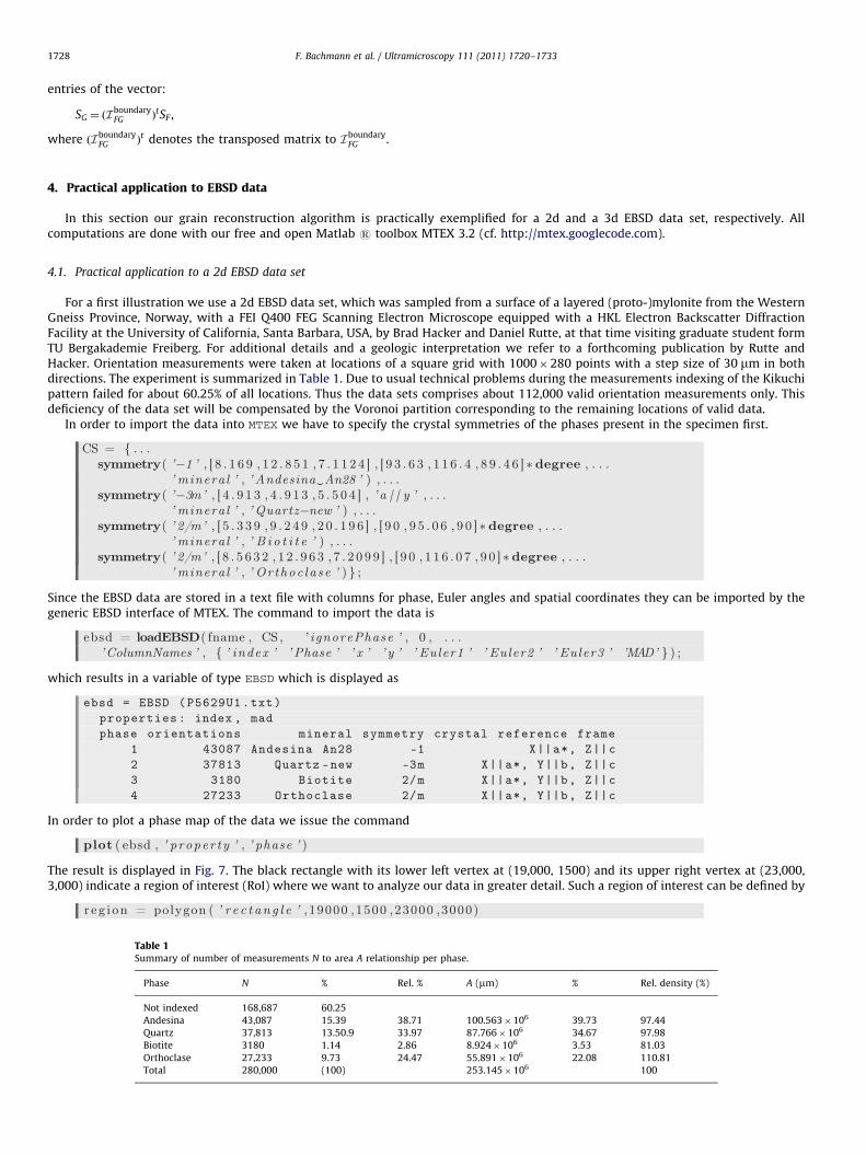
For a first illustration we use a 2d EBSD data set, which was sampled from a surface of a layered (proto-)mylonite from the WesternGneiss Province, Norway, with a FEI Q400 FEG Scanning Electron Microscope equipped with a HKL Electron Backscatter DiffractionFacility at the University of California, Santa Barbara, USA, by Brad Hacker and Daniel Rutte, at that time visiting graduate student formTU Bergakademie Freiberg. For additional details and a geologic interpretation we refer to a forthcoming publication by Rutte andHacker. Orientation measurements were taken at locations of a square grid with 1000�280 points with a step size of 30 mm in bothdirections. The experiment is summarized in Table 1. Due to usual technical problems during the measurements indexing of the Kikuchipattern failed for about 60.25% of all locations. Thus the data sets comprises about 112,000 valid orientation measurements only. Thisdeficiency of the data set will be compensated by the Voronoi partition corresponding to the remaining locations of valid data.

In order to import the data into MTEX we have to specify the crystal symmetries of the phases present in the specimen first.

Since the EBSD data are stored in a text file with columns for phase, Euler angles and spatial coordinates they can be imported by thegeneric EBSD interface of MTEX. The command to import the data is

which results in a variable of type EBSD which is displayed as

In order to plot a phase map of the data we issue the command

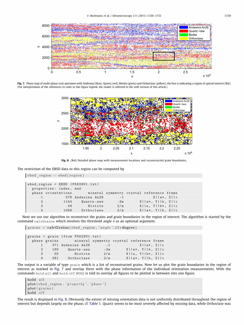
The result is displayed in Fig. 7. The black rectangle with its lower left vertex at (19,000, 1500) and its upper right vertex at (23,000,3,000) indicate a region of interest (RoI) where we want to analyze our data in greater detail. Such a region of interest can be defined by

Table 1Summary of number of measurements N to area A relationship per phase.

Phase N % Rel. % A (mm) % Rel. density (%)

Not indexed 168,687 60.25

Andesina 43,087 15.39 38.71 100.563�106 39.73 97.44

Quartz 37,813 13.50.9 33.97 87.766�106 34.67 97.98

Biotite 3180 1.14 2.86 8.924�106 3.53 81.03

Orthoclase 27,233 9.73 24.47 55.891�106 22.08 110.81

Total 280,000 (100) 253.145�106 100

x

y

0 0.5 1 1.5 2 2.5x 104

0

2000

4000

6000

8000 Andesina An28Quartz−newBiotiteOrthoclase

Fig. 7. Phase map of multi-phase rock specimen with Andesina (blue), Quartz (red), Biotite (green) and Orthoclase (yellow), the box is indicating a region of special interest (RoI).

(For interpretation of the references to color in this figure legend, the reader is referred to the web version of this article.)

x

y

1.95 2 2.05 2.1 2.15 2.2 2.25x 104

1500

2000

2500

3000Andesina An28Quartz−newBiotiteOrthoclase

Fig. 8. (RoI) Detailed phase map with measurement locations and reconstructed grain boundaries.

F. Bachmann et al. / Ultramicroscopy 111 (2011) 1720–1733 1729

The restriction of the EBSD data to this region can be computed by

Next we use our algorithm to reconstruct the grains and grain boundaries in the region of interest. The algorithm is started by thecommand calcGrains which involves the threshold angle d as an optional argument.

The output is a variable of type grain which is a list of reconstructed grains. Now let us plot the grain boundaries in the region ofinterest as marked in Fig. 7 and overlay them with the phase information of the individual orientation measurements. With thecommands hold all and hold off MTEX is told to overlay all figures to be plotted in between into one figure.

The result is displayed in Fig. 8. Obviously the extent of missing orientation data is not uniformly distributed throughout the region ofinterest but depends largely on the phase, cf. Table 1. Quartz seems to be most severely affected by missing data, while Orthoclase was

F. Bachmann et al. / Ultramicroscopy 111 (2011) 1720–17331730

more successfully indexed than the average as realized for Andesina and Quartz. Thus, to the largest extent, Quartz grains to bedetermined will depend on the buffering of measurement locations to Voronoi cells.

Fig. 9 displays the reconstructed grain boundaries together with the individual orientation measurement of quartz and demonstratesthat beside the large extend of missing data the modeled grains match the data. The plot was created with the commands

These commands exemplify how to use various options. By grains({‘An’,‘Bi’,‘Or’}) we select from all grains only those of phaseAndesina, Biotite, and Orthoclase any by ebsd_region(‘Qu’) we select only the EBSD data of phase Quartz. The option FaceAlpha can beused to shade down the output of the specific command. The EBSD measurements of the Quartz phase are colored according to theirorientation, which in turn is color coded with respect to the color map provided by the (001) inverse pole figure (see Fig. 9b).

Next we want to plot the Quartz grains colored according to the mean orientation. This is done by the commands:

The result is shown in Fig. 10.Once grain boundaries have been reconstructed, they may be classified according to some criteria, e.g. small vs. large angle

boundaries by thresholding, or by checking the misorientation of adjacent grains for some specific relationships. In Fig. 11 grain

Fig. 9. (RoI) Individual orientation measurements of quartz together with the grain boundaries. (a) Orientation map. (b) Color map. (For interpretation of the references to

color in this figure legend, the reader is referred to the web version of this article.)

Fig. 10. (RoI) The reconstructed grains. The quartz grains are colored according to their mean orientation while the remaining grains are colored according to there phase.

(a) Orientation map. (b) Color map.

Fig. 11. (RoI A) Phase map with grain boundaries highlighted, where adjacent grains have a misorientation with rotational axis close to the c-axis.

F. Bachmann et al. / Ultramicroscopy 111 (2011) 1720–1733 1731

boundaries are highlighted, where the misorientation of their adjacent grains is a rotation about the c-axis with an allowed tolerance of5 degrees. Fig. 11 was accomplished with the commands

4.2. Practical application to a 3d EBSD data set

In this section we apply our algorithm to 3d EBSD data which were collected from a low-carbon steel specimen with a dual beam FIB(focused ion beam) scanning electron microscope of the type FEI NOVA600-Nanolab(r). The data were recorded at the Materials Scienceand Engineering Department of Ghent University by the group of Kestens and Petrov, cf. [15–17]. Orientation measurements were takenat locations of registered planar square grids with a stepsize of 0:1 mm in both directions and a spacing of equidistant planes of 0:12 mm.The data sets comprises 140�160�59 orientation measurements. In order to import the data into MTEX we first specify thez-coordinates of the slices and then call the command loadEBSD with the name of the directory containing the data files.

The data can be visualized by plotting the individual orientations on slices passing through the measured cube. In MTEX this can beinteractively done by the command

The resulting plot is shown in Fig. 12a.Since the data set is perfectly complete, computations to determine the 3d Voronoi cells is not required but instead partition into cube

volume elements (‘‘voxels’’) applies. With the only difference that in this special case grains are composed of voxels, the determination ofgrains and grain boundaries is analogously to the two dimensional case.

In order to visualize the grains we first restrict ourself to 43 mid-sized grains by

Fig. 12. View of 3d solid grain model based on EBSD data from serial sectioning (left), and slicing the 3d grain model (right). (a) Slices and (b) Grains.

Fig. 13. View of an individual grain with sub-boundaries; lines of intersection of boundaries and sub-boundaries are marked in red, and two planes of sectioning are

marked in cyan and yellow, respectively (left). While the section by the plane depicted in cyan suggests a set of adjacent grains (center), the section by the plane depicted

in yellow indicates spatially separated grains (right). (a) 3d plot, (b) section A, (c) section B. (For interpretation of the references to color in this figure legend, the reader is

referred to the web version of this article.)

F. Bachmann et al. / Ultramicroscopy 111 (2011) 1720–17331732

Then we plot these grains by the command

The result is shown in Fig. 12b.In Fig. 13 a single grain is plotted from different points of view. In Fig. 13a, a three 3d views of the grain are shown, whereas its

intersections with two different planes are displayed in Fig. 13b and c. What appears as a hole in Fig. 13a of the 3d model makes the grainappear as two or more separated grains in Fig. 13c.

A completely worked out example considering 3d EBSD data will be included in the on-line documentation and ready for download.For the time being there is only little experience of interpretation and quantitative evaluation of 3d views of the fabric, e.g. with respectto the parametrization of grain boundaries in terms of location, crystallographic misorientation, and spatial orientation of the face by itsunit normal vector. Future discussions within the texture and fabric community will clarify which properties derived from 3d EBSD dataare crucial and how they should be visualized to facilitate expert interpretation and inference.

5. Conclusions

A novel general approach to grain boundary reconstruction based on explicit mathematical modeling assumptions and employingVoronoi decomposition of the domain of measurement locations has been presented. Its major advantages are that

�

it applies to EBSD data in 2d or 3d domains, � it is invariant with respect to translation and rotation of the specimen, � it does not require interpolation of orientation measurements to substitute poorly indexed or missing orientation data, � it is fast, i.e., the order of magnitude of computer time of the algorithms used in MTEX is almost linear.

F. Bachmann et al. / Ultramicroscopy 111 (2011) 1720–1733 1733

Spatial modeling of grains and grain boundaries opens the route towards comprehensive fabric analysis as envisioned by BrunoSander [22], e.g. it is a prerequisite of orientation statistics per grain as developed in [9], and to misorientation analysis with respect to

neighboring grains, also included in MTEX. All computations are done with our free and open Matlab s toolbox MTEX 3.2 [24].

Acknowledgments

The authors would like to thank Brad R. Hacker, Professor of Earth Science at the Earth Research Institute of the University ofCalifornia, Santa Barbara, USA, and Daniel Rutte, TU Bergakademie Freiberg and former visiting graduate student at UC Santa Barbara, forthe 2d EBSD data set of a mylonite, and Leo Kestens, Professor of Metal Science and Technology with the Department of Materials Scienceand Engineering at Ghent University, Belgium, for the 3d EBSD data set from a low-carbon steel specimen. The senior author (HS) wouldlike to thank Fundac- ~ao Coordenac- ~ao de Aperfeic-oamento de Pessoal de Nıvel (CAPES) and German Academic Exchange Service (DAAD)for funding a three months research stay at Centro de Microscopia da Universidade Federal de Minas Gerais in Belo Horizonte, Brazil,with Prof. Karla Balzuweit and Prof. Carlos A. Rosi�ere, during which this paper was completed.

References

[1] B.L. Adams, S.I. Wright, K. Kunze, Orientation imaging: The emergency of a new microscopy, Metallurgy Transactions 24A (1993) 819–831.[2] K. Kunze, S.I. Wright, B.L. Adams, D.J. Dingley, Advances in automatic EBSP single orientation measurements, Textures and Microstructures 20 (1993) 41–54.[3] A. Rollett, S. Lee, R. Campman, G. Roherer, Three dimensional characterization of microstructure by electron back-scatter diffraction, Annual Review of Material

Research 37 (2007) 627–658.[4] P.S. Bate, R.D. Knutsen, I.B. Rough, F.J. Humphreys, The characterization of low-angle boundaries by EBSD, Journal of Microscopy 220 (2005) 36–46.[5] R. Heilbronner, Automatic grain boundary detection and grain size analysis using polarization micrographs or orientation images, Journal of Structural Geology

22 (2000) 969–981.[6] Y. Li, C.M. Onasch, Y. Guo, GIS-based detection of grain boundaries, Journal of Structural Geology 30 (2008) 431–443.[7] A.K. Kulshreshth, A. Alpers, T.G. Herman, E. Knudsen, L. Rodek, H.F. Poulsen, A greedy method for reconstructing polycrystals from three-dimensional x-ray diffraction

data, Inverse Problems and Imaging 3 (2009) 69–85.[8] A. Melcher, A. Unser, M. Reichhardt, B. Nestler, M. Potschke, M. Selzer, Conversion of EBSD data by a quaternion based algorithm to be used for grain structure

simulations, Technische Mechanik 30 (2010) 401–413.[9] F. Bachmann, R. Hielscher, P.E. Jupp, W. Pantleon, S. Schaeben, E. Wegert, Inferential statistics of EBSD data from within individual crystalline grains, Journal of Applied

Crystallography 43 (2010) 1338–1355.[10] R. Hielscher, H. Schaben, A novel pole figure inversion method: specification of the MTEX algorithm, Journal of Applied Crystallography 41 (2008) 1024–1037.[11] R. Hielscher, Kernel density estimation on the rotation group. Preprint 2010-7, FakultAd’t fAijr Mathematik, TU Chemnitz, 2010.[12] D. Mainprice, R. Hielscher, H. Schaeben, Calculating anisotropic physical properties from texture data using the MTEX open source package, Society, 1–33, in:

D.J. Prior, E.H. Rutter, D.J Tatham (Eds.), Deformation Mechanisms, Rheology and Tectonics: Microstructures, Mechanics and Anisotropy, 360, Geological Society,London, 2011, pp. 175–192 doi: 10.1144/SP360.10 (Special publications).

[14] R. Hielscher, H. Schaeben, H. Siemes, Orientation Distribution Within a Single Hematite Crystal, Mathematical Geosciences 42 (2010) 375–395.[15] R. Petrov, O.L. Garcia, J.J.L. Mulders, A.C. Reis, J.-H. Bae, L. Kestens, Y. Houbaert, Three dimensional microstructure-microtexture characterisation of pipeline steel, in:

P.B. Prangnell, P.S. Bate (Eds.), Fundamentals of Deformation and Annealing, 550, Materials Science Forum, 2007, pp. 625–630.[16] R. Petrov, O.L. Garcia, H. Sharma, P.G. Hernandez, L. Kestens, 3D-microstructure and texture characterization in different length scales, in: A.D. Rollet, (Ed.), Applications of

Texture Analysis, Ceramic Transactions 201A, Collection of Papers Presented at the 15th International Conference on Texture in Materials (ICOTOM 15), June 1–6, 2008Pittsburgh, Pennsylvania, USA, 2008, pp. 197–204.

[17] O.L. Garcia, R. Petrov, L. Kestens, Local characterization of void initiation on IF steel by FIB-EBSD technique in: A.D. Rollet (Ed.), Applications of Texture Analysis,Ceramic Transactions 201A, Collection of Papers Presented at the 15th International Conference on Texture in Materials (ICOTOM 15), June 1–6, 2008 Pittsburgh,Pennsylvania, USA, 2008, pp. 693–700.

[18] O. Melnikov, R. Tyshkevich, V. Yemelichev, V. Sarvanov, Lectures on Graph Theory, Nauka, Moscow, 1990.[19] G.L. Dirichlet, Uber die Reduktion der positiven quadratischen Formen mit drei unbestimmten ganzen Zahlen, Journal fur die Reine und Angewandte Mathematik

40 (1850) 209–227.[20] G. Voronoi, Nouvelles applications des paramtres continus la thorie des formes quadratiques, Journal fr die Reine und Angewandte Mathematik 133 (1907) 97–178.[21] B. Barber, D.P. Dobkin, H. Huhdanpaa, The Quickhull algorithm for convex hulls, ACM Transactions on Mathematical Software 22 (1996) 469–483.[22] B. Sander, Gefugekunde der Gesteine, Springer, Vienna, 1930.[24] R. Hielscher, F. Bachmann, MTEX 3.2 – A Texture Calculation Toolbox, /http://mtex.googlecode.comS, 2011.