1 Graph Theory and Topology Design David Tipper Associate Professor Associate Professor Graduate Telecommunications and Networking Program University of Pittsburgh [email protected][email protected]Slides 4 Slides 4 http://www.sis.pitt.edu/~dtipper/2110.html • Top down network design project approach should follow three phases: – Conceptual Model Top Down Network Design Approach Conceptual Model • Objectives, Requirements, Constraints – Logical Model • Technology, network graph, node location, link size, etc. (where algorithms are used to minimize cost) – Physical Model • Specific hardware/software implementations ( ii di t l ti t ) Telcom 2110 2 • (e.g., wiring diagram, repeater locations, etc.) • Focus on Algorithms for Logical Model Design – Graph Theory – Optimization
Transcript
1
Graph Theory and Topology Design
David TipperAssociate ProfessorAssociate Professor
Graduate Telecommunications and Networking ProgramUniversity of Pittsburgh
• Focus on Algorithms for Logical Model Design– Graph Theory– Optimization
2
Graphs
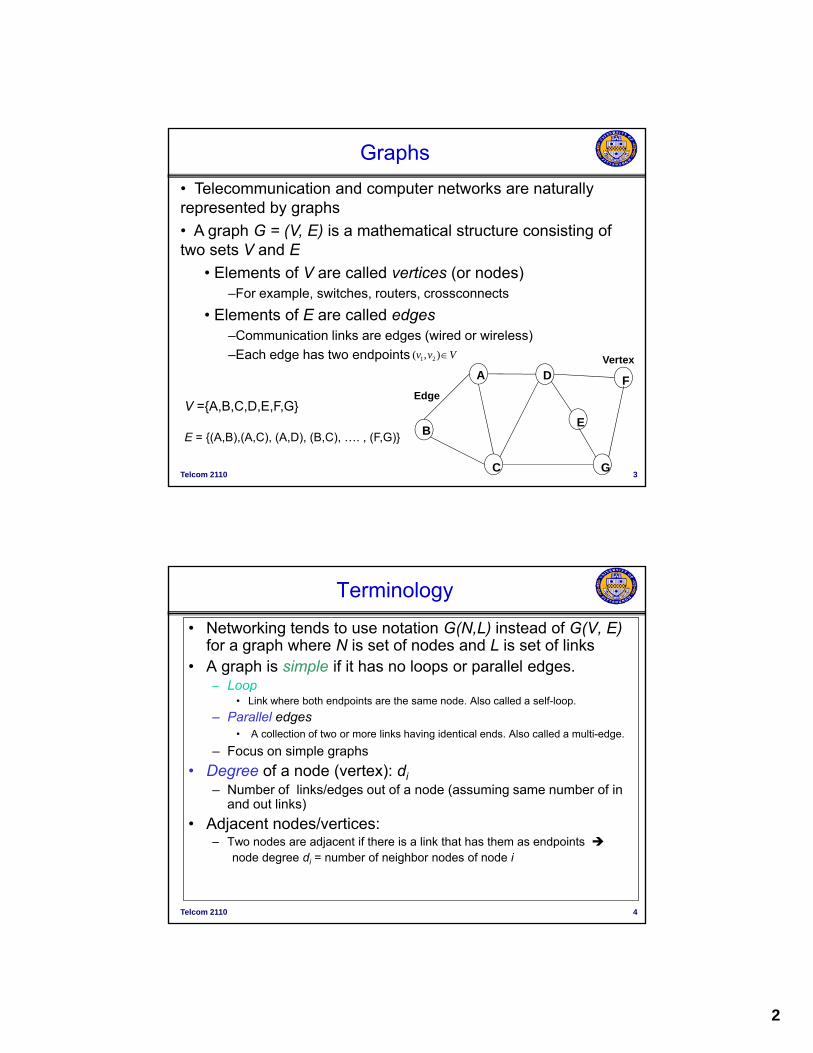
• Telecommunication and computer networks are naturally represented by graphs
• A graph G = (V, E) is a mathematical structure consisting of two sets V and Etwo sets V and E
• Elements of V are called vertices (or nodes)–For example, switches, routers, crossconnects
• Elements of E are called edges –Communication links are edges (wired or wireless)
–Each edge has two endpoints VertexVvv ),( 21
Telcom 2110 3
A
B
C
D
E
F
G
V ={A,B,C,D,E,F,G}
E = {(A,B),(A,C), (A,D), (B,C), …. , (F,G)}
Edge
Terminology
• Networking tends to use notation G(N,L) instead of G(V, E)for a graph where N is set of nodes and L is set of links
• A graph is simple if it has no loops or parallel edges.Loop– Loop
• Link where both endpoints are the same node. Also called a self-loop.
– Parallel edges• A collection of two or more links having identical ends. Also called a multi-edge.
– Focus on simple graphs
• Degree of a node (vertex): di– Number of links/edges out of a node (assuming same number of in
and out links)
Telcom 2110 4
and out links)
• Adjacent nodes/vertices:– Two nodes are adjacent if there is a link that has them as endpoints
node degree di = number of neighbor nodes of node i
3
A D F
Terminology Cont.
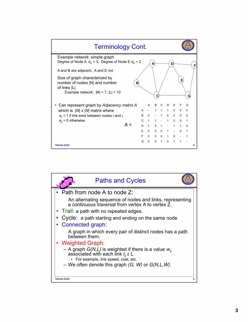
Example network: simple graph Degree of Node A dA = 3, Degree of Node E dE = 2
A and B are adjacent, A and E not
B
C
E
G
• Can represent graph by Adjacency matrix Awhich is |N| x |N| matrix where
Size of graph characterized by number of nodes |N| and numberof links |L|
Example network: |N| = 7, |L| = 10
A B C D E F G
A - 1 1 1 0 0 0
Telcom 2110 5
| | | |aij = 1 if link exist between nodes i and j aij = 0 otherwise
B 0 - 1 0 0 0 0
C 1 1 - 1 0 0 1
D 1 0 1 - 1 1 0
E 0 0 0 1 - 0 1
F 0 0 0 1 0 - 1
G 0 0 1 0 1 1 -
A =
Paths and Cycles
• Path from node A to node Z: An alternating sequence of nodes and links, representing a continuous traversal from vertex A to vertex Z.
T il th ith t d d• Trail: a path with no repeated edges.
• Cycle: a path starting and ending on the same node
• Connected graph:A graph in which every pair of distinct nodes has a path between them.
• Weighted Graph:
Telcom 2110 6
– A graph G(N,L) is weighted if there is a value wijassociated with each link lij ɛ L
• For example, link speed, cost, etc.
– We often denote this graph (G, W) or G(N,L,W).
4
Terminology Cont.
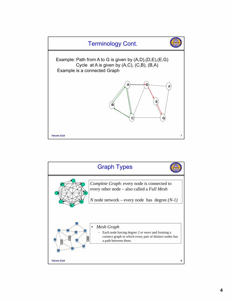
Example: Path from A to G is given by (A,D),(D,E),(E,G)Cycle at A is given by (A,C), (C,B), (B,A)
Example is a connected Graph
A
B
D
E
F
Example is a connected Graph
Telcom 2110 7
B
C G
Graph Types
Complete Graph: every node is connected to every other node – also called a Full Mesh
N node network – every node has degree (N-1)
• Mesh Graph
Telcom 2110 8
– Each node having degree 2 or more and forming a connect graph in which every pair of distinct nodes has a path between them.
5
Graph Types
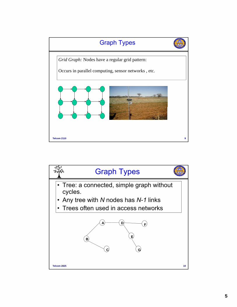
Grid Graph: Nodes have a regular grid pattern:
Occurs in parallel computing, sensor networks , etc.Occurs in parallel computing, sensor networks , etc.
Telcom 2110 9
Graph Types
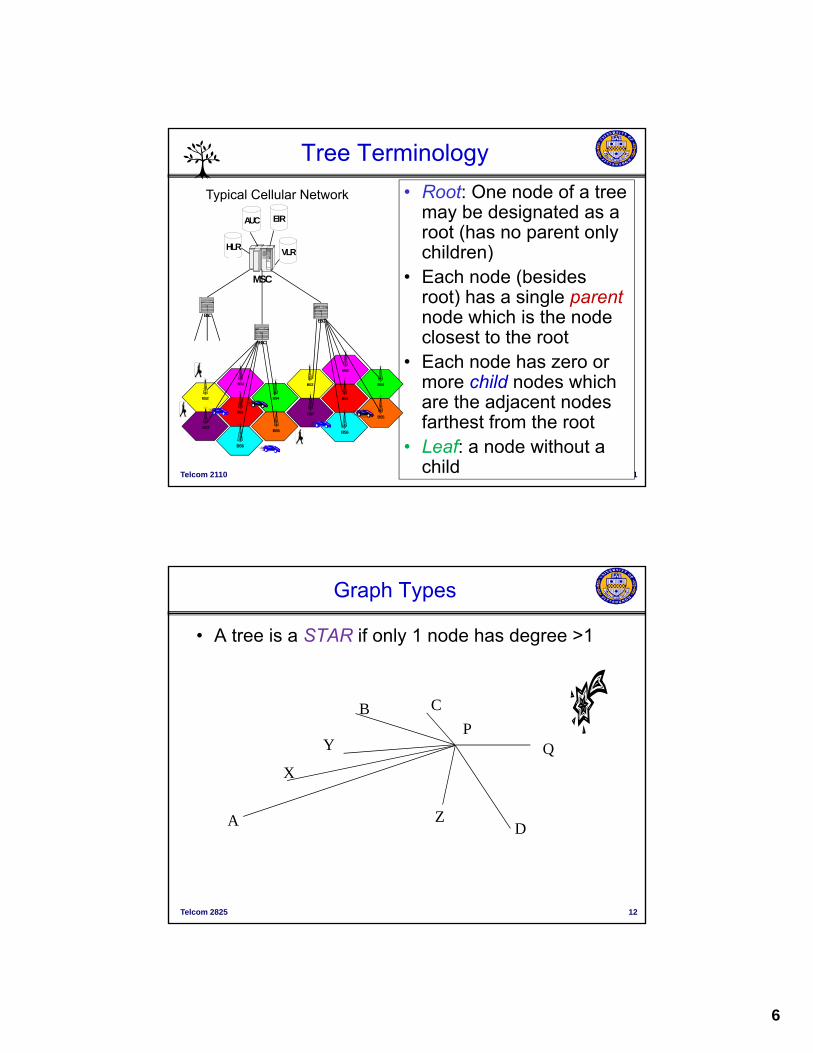
• Tree: a connected, simple graph without cycles.
• Any tree with N nodes has N 1 links• Any tree with N nodes has N-1 links• Trees often used in access networks
A D F
Telcom 2825 10
C G
BE
6
Tree Terminology
• Root: One node of a tree may be designated as a root (has no parent only hild )HLR
AUC EIR
Typical Cellular Network
children)• Each node (besides
root) has a single parentnode which is the node closest to the root
• Each node has zero or
IBM
MSC
SD
Centillion 1400Bay Networks
ETHER RS 232C
PC CARD
P*8x50
O OO130A O N
6
INS ACT ALMRST LINK
PWR ALM FAN 0 FAN1 PWR0 PWR1
ALM
BSCSD
Centillion 1400Bay Networks
ETHER RS 232C
PC CARD
P*8x50
O OO130A O N
6
INS ACT ALMRST LINK
PWR ALM FAN 0 FAN1 PWR0 PWR1
ALM
BSC
SD
Centillion 1400Bay Networks
ETHER RS 232C
PC CARD
P*8x50OOO130
A O N6
INS ACT ALMR ST LINK
PWR ALM FAN0 FAN1 PWR 0PWR1
ALM
BSC
VLRHLR
Telcom 2110 11
Each node has zero or more child nodes which are the adjacent nodes farthest from the root
• Leaf: a node without a child
BS7BS5
BS2
BS3
BS4
BS1
BS6BS7
BS5
BS2
BS3
BS4
BS1
BS6
Graph Types
• A tree is a STAR if only 1 node has degree >1
X
YP
Q
B C
Telcom 2825 12
ZA D
7
Graph Types
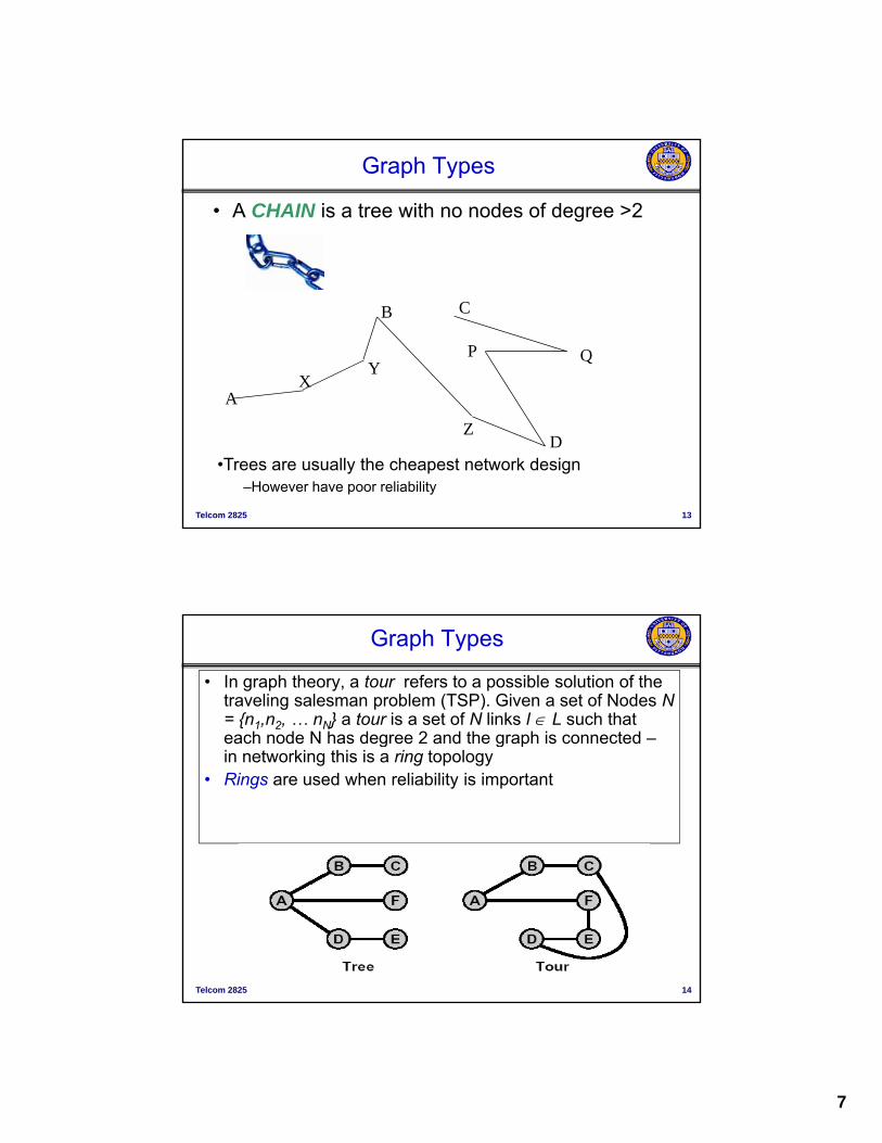
• A CHAIN is a tree with no nodes of degree >2
XY
P Q
A
B C
Telcom 2825 13
Z
A
D•Trees are usually the cheapest network design
–However have poor reliability
Graph Types
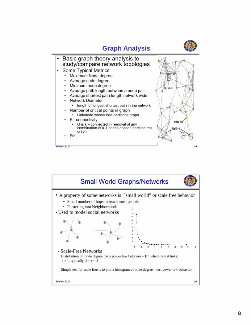
• In graph theory, a tour refers to a possible solution of the traveling salesman problem (TSP). Given a set of Nodes N = {n1,n2, … nN} a tour is a set of N links l L such that each node N has degree 2 and the graph is connected –eac ode as deg ee a d t e g ap s co ectedin networking this is a ring topology
• Rings are used when reliability is important
Telcom 2825 14
8
Graph Analysis
• Basic graph theory analysis to study/compare network topologies
• Some Typical Metrics• Maximum Node degreeMaximum Node degree• Average node degree• Minimum node degree• Average path length between a node pair• Average shortest path length network wide• Network Diameter
• length of longest shortest path in the network• Number of critical points in graph
Telcom 2110 15
• Link/node whose loss partitions graph• K –connectivity
• G is k – connected in removal of any combination of k-1 nodes doesn’t partition the graph
• Etc..
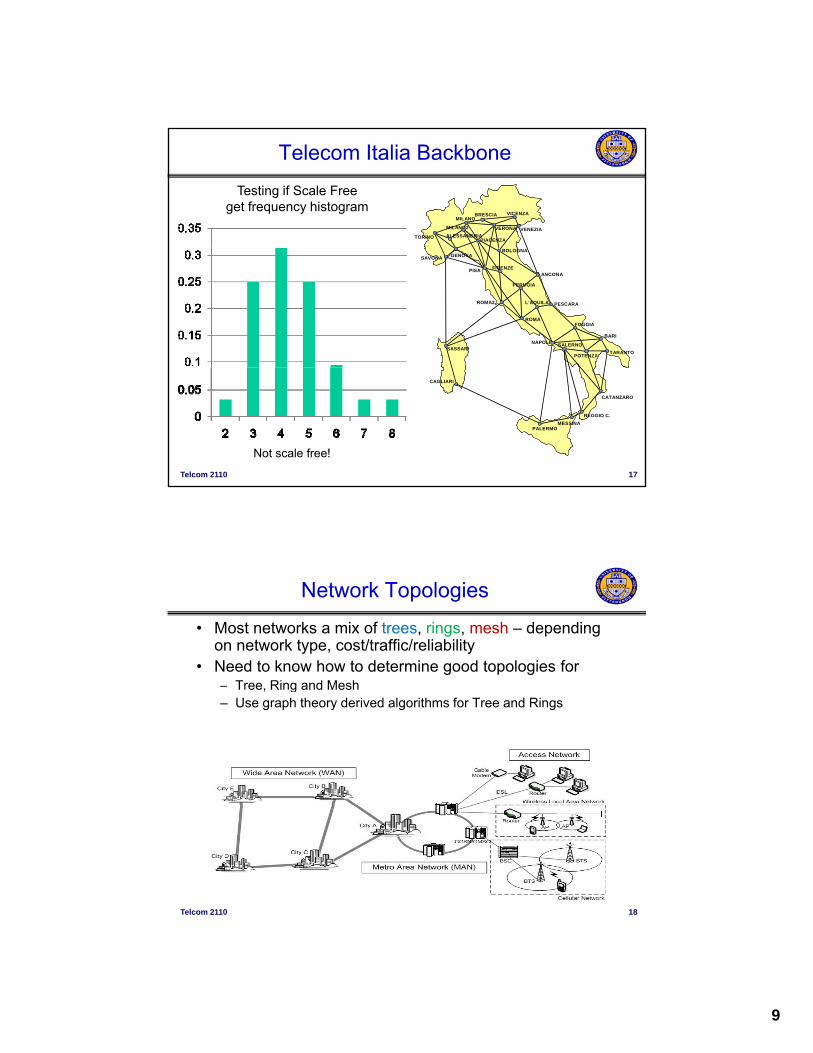
Small World Graphs/Networks
• A property of some networks is ``small world” or scale free behavior• Small number of hops to reach most people• Clustering into Neighborhoods
U d t d l i l t k• Used to model social networks
Telcom 2110 16
• Scale-Free Networks Distribution of node degree has a power law behavior ~ k-r where k = # links; r > 1, typically 2 < r < 3
Simple test for scale free is to plot a histogram of node degree – test power law behavior
9
Telecom Italia Backbone
TORINO ALESSANDRIA
MILANOBRESCIA
VERONA
VICENZA
VENEZIA
PIACENZA
MILANO2
Testing if Scale Freeget frequency histogram
GENOVA
PISA
SAVONA
BOLOGNA
FIRENZEANCONA
PESCARA
PERUGIA
L’AQUILA
ROMA
ROMA2
NAPOLI SALERNO
POTENZA
BARI
TARANTOSASSARI
FOGGIA
Telcom 2110 17
CATANZARO
CAGLIARI
PALERMOMESSINA
REGGIO C.
Not scale free!
Network Topologies
• Most networks a mix of trees, rings, mesh – depending on network type, cost/traffic/reliability
• Need to know how to determine good topologies for Tree Ring and Mesh– Tree, Ring and Mesh
– Use graph theory derived algorithms for Tree and Rings
Telcom 2110 18
10
Design of Trees
• Many algorithms for design and types of trees – Minimum Spanning Trees, Shortest Path Trees, etc.
• Spanning Trees and SubgraphsSpanning Trees and Subgraphs– Subgraph of graph G obtained by selecting number of
links and nodes from G• For each link, the two nodes incident on that link must be
selected
– Give graph G(N,L), graph G’(N’,L’) is a subgraph of G iffN’ N and L’ L and
Telcom 2110 19
N N and L L and
l’ L’, if l’ incident on e’ and w’ then e’, w’ N’
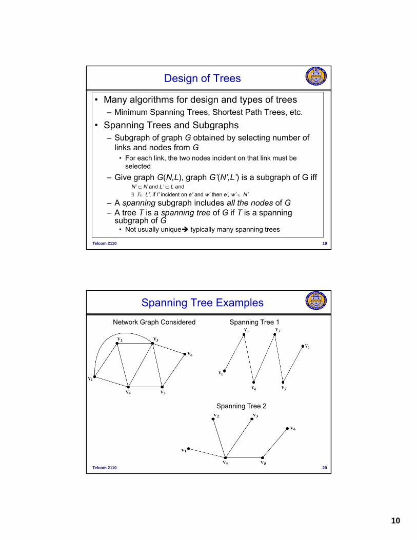
– A spanning subgraph includes all the nodes of G– A tree T is a spanning tree of G if T is a spanning
subgraph of G• Not usually unique typically many spanning trees
Spanning Tree Examples
Network Graph Considered Spanning Tree 1
Spanning Tree 2
Telcom 2110 20
11
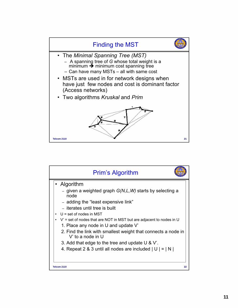
Finding the MST
• The Minimal Spanning Tree (MST)– A spanning tree of G whose total weight is a
minimum minimum cost spanning tree – Can have many MSTs – all with same costCan have many MSTs all with same cost
• MSTs are used in for network designs when have just few nodes and cost is dominant factor (Access networks)
• Two algorithms Kruskal and Prim
Telcom 2110 21
Prim’s Algorithm
• Algorithm – given a weighted graph G(N,L,W) starts by selecting a
nodeddi th “l t i li k”– adding the “least expensive link”
– iterates until tree is built• U = set of nodes in MST
• V’ = set of nodes that are NOT in MST but are adjacent to nodes in U
1. Place any node in U and update V’2. Find the link with smallest weight that connects a node in
V’ t d i U
Telcom 2110 22
V’ to a node in U3. Add that edge to the tree and update U & V’.4. Repeat 2 & 3 until all nodes are included | U | = | N |
12
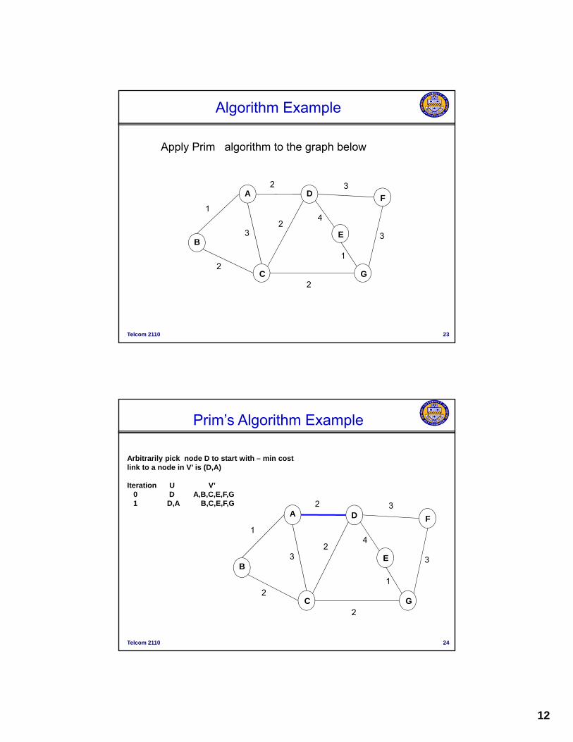
Apply Prim algorithm to the graph below
Algorithm Example
A
B
D
E
F1
3
2
24
1
3
3
Telcom 2110 23
C G2
2
Arbitrarily pick node D to start with – min cost link to a node in V’ is (D,A)
It ti U V’
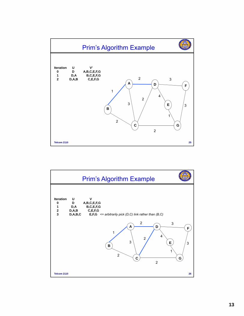
Prim’s Algorithm Example
A
B
D
E
F1
3
2
24
3
3
Iteration U V’0 D A,B,C,E,F,G1 D,A B,C,E,F,G
Telcom 2110 24
B
C G2
2
1
13
Prim’s Algorithm Example
Iteration U V’0 D A,B,C,E,F,G1 D A B C E F G
A
B
D
E
F
1
3
2
24
3
3
1 D,A B,C,E,F,G2 D,A,B C,E,F,G
Telcom 2110 25
C G2
2
1
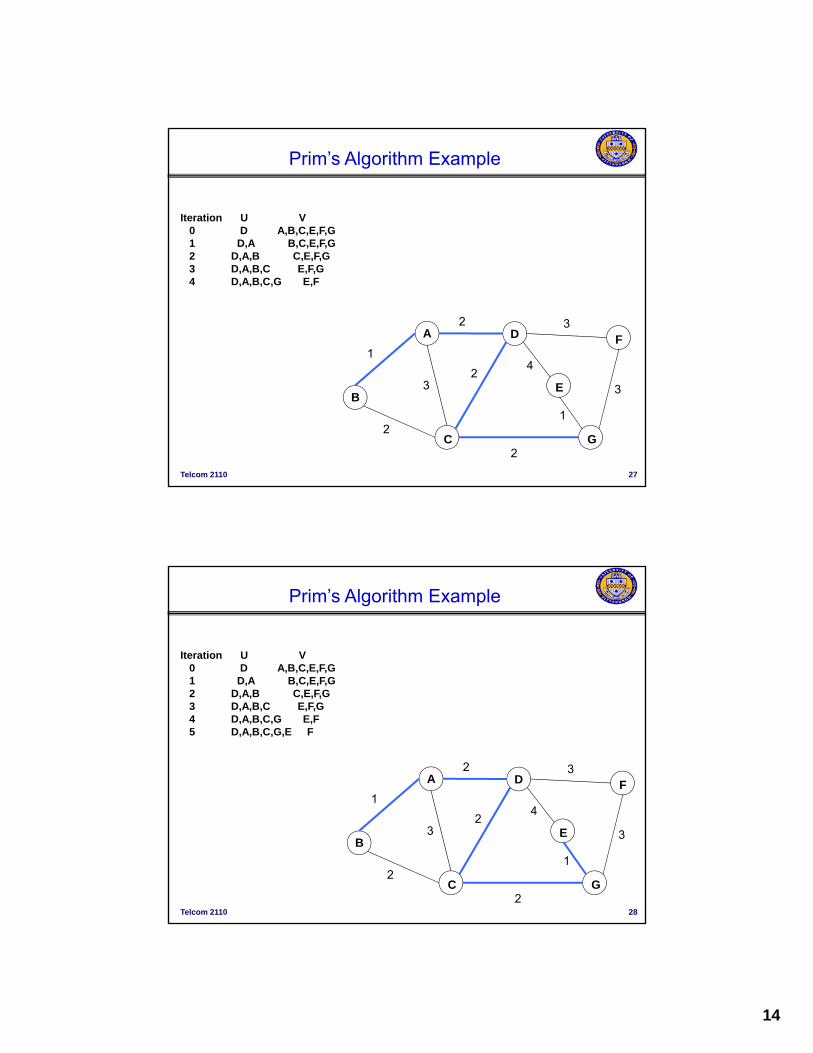
Prim’s Algorithm Example
Iteration U V0 D A,B,C,E,F,G1 D A B C E F G
A D
E
F1
3
2
24
3
1 D,A B,C,E,F,G2 D,A,B C,E,F,G3 D,A,B,C E,F,G <= arbitrarily pick (D,C) link rather than (B,C)
Iteration U V’0 D A,B,C,E,F,G1 D,A B,C,E,F,G2 D,A,B C,E,F,G
A D F1
2 3
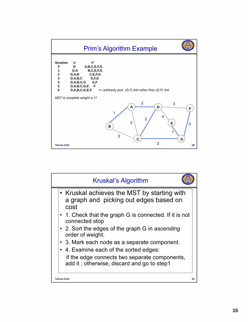
, , , , ,3 D,A,B,C E,F,G 4 D,A,B,C,G E,F5 D,A,B,C,G,E F6 D,A,B,C,G,E,F <= arbitrarily pick (G,F) link rather than (D,F) link
MST is complete weight is 11
Telcom 2110 29
B
C
E
G
1
2
32
2
4
1
3
Kruskal’s Algorithm
• Kruskal achieves the MST by starting with a graph and picking out edges based on cost
• 1. Check that the graph G is connected. If it is not connected stop
• 2. Sort the edges of the graph G in ascending order of weight.
• 3. Mark each node as a separate component.
Telcom 2110 30
• 4. Examine each of the sorted edges:if the edge connects two separate components, add it ; otherwise, discard and go to step1
16
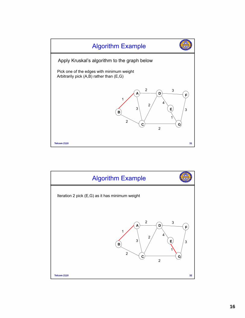
Apply Kruskal’s algorithm to the graph below
Algorithm Example
Pick one of the edges with minimum weight A bi il i k (A B) h h (E G)
A
B
D
E
F1
3
2
24
3
3
Arbitrarily pick (A,B) rather than (E,G)
Telcom 2110 31
B
C G2
2
1
3
Algorithm Example
Iteration 2 pick (E,G) as it has minimum weight
A
B
D
E
F1
3
2
24
3
3
Telcom 2110 32
B
C G2
2
1
3
17
Algorithm Example
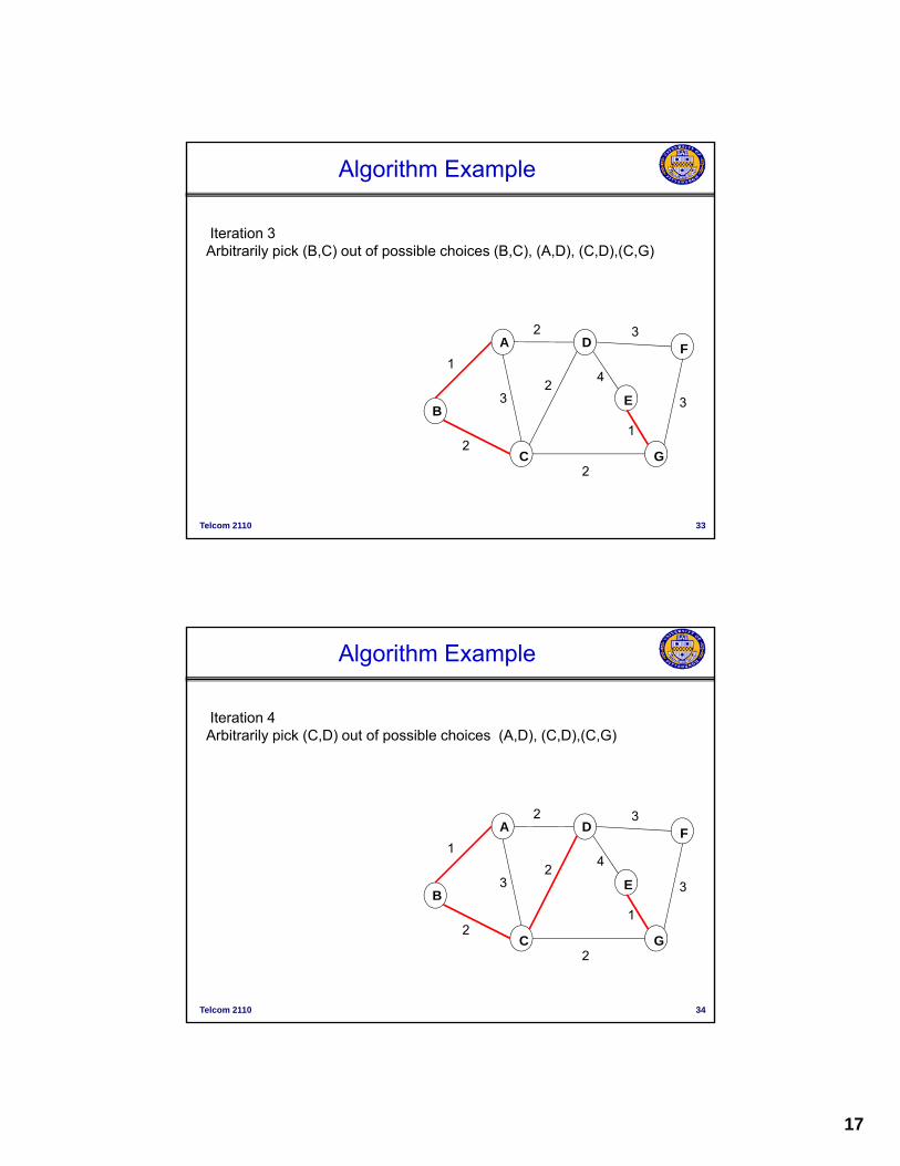
Iteration 3 Arbitrarily pick (B,C) out of possible choices (B,C), (A,D), (C,D),(C,G)
A
B
D
E
F1
3
2
24
3
3
Telcom 2110 33
B
C G2
2
1
3
Algorithm Example
Iteration 4 Arbitrarily pick (C,D) out of possible choices (A,D), (C,D),(C,G)
A
B
D
E
F1
3
2
24
3
3
Telcom 2110 34
B
C G2
2
1
3
18
Algorithm Example
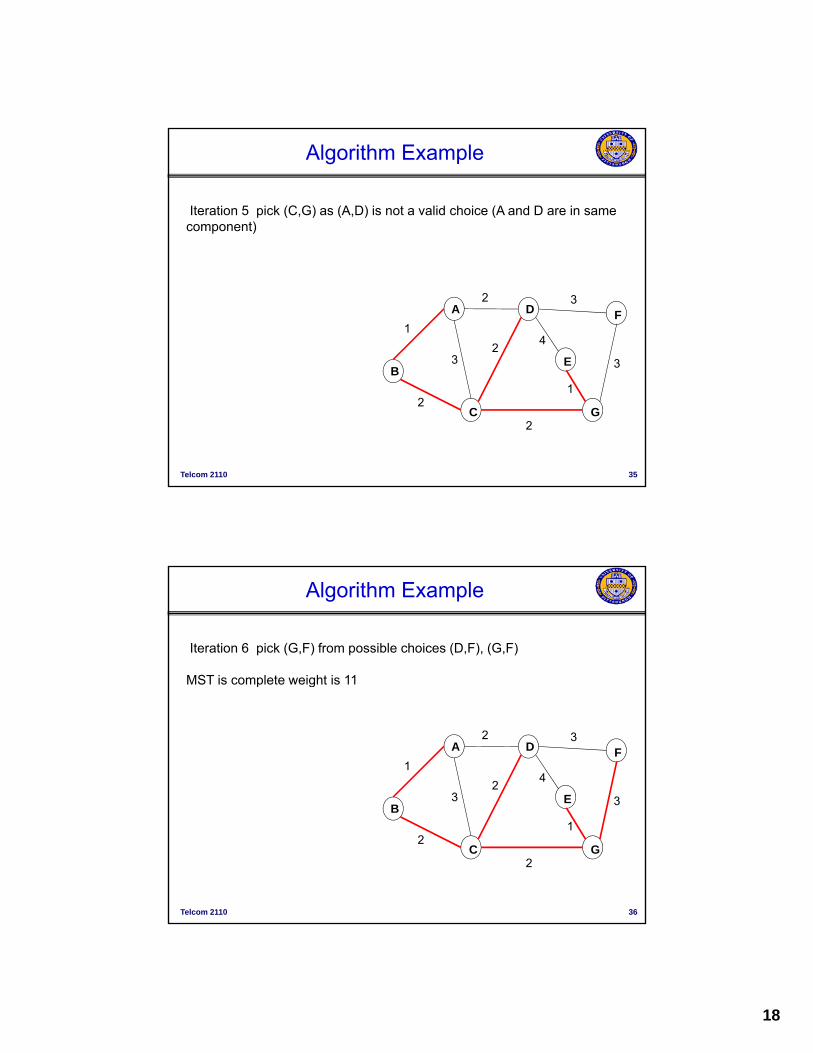
Iteration 5 pick (C,G) as (A,D) is not a valid choice (A and D are in same component)
A
B
D
E
F1
3
2
24
3
3
Telcom 2110 35
B
C G2
2
1
3
Algorithm Example
Iteration 6 pick (G,F) from possible choices (D,F), (G,F)
MST is complete weight is 11
A
B
D
E
F1
3
2
24
3
3
p g
Telcom 2110 36
B
C G2
2
1
3
19
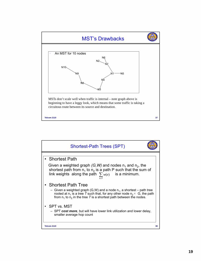
• An MST for 10 nodesN6
N2
MST’s Drawbacks
N2 N7
N10
N9 N1 N5
N4N8
N3
Telcom 2110 37
MSTs don’t scale well when traffic is internal – note graph above is beginning to have a leggy look, which means that some traffic is taking a circuitous route between its source and destination.
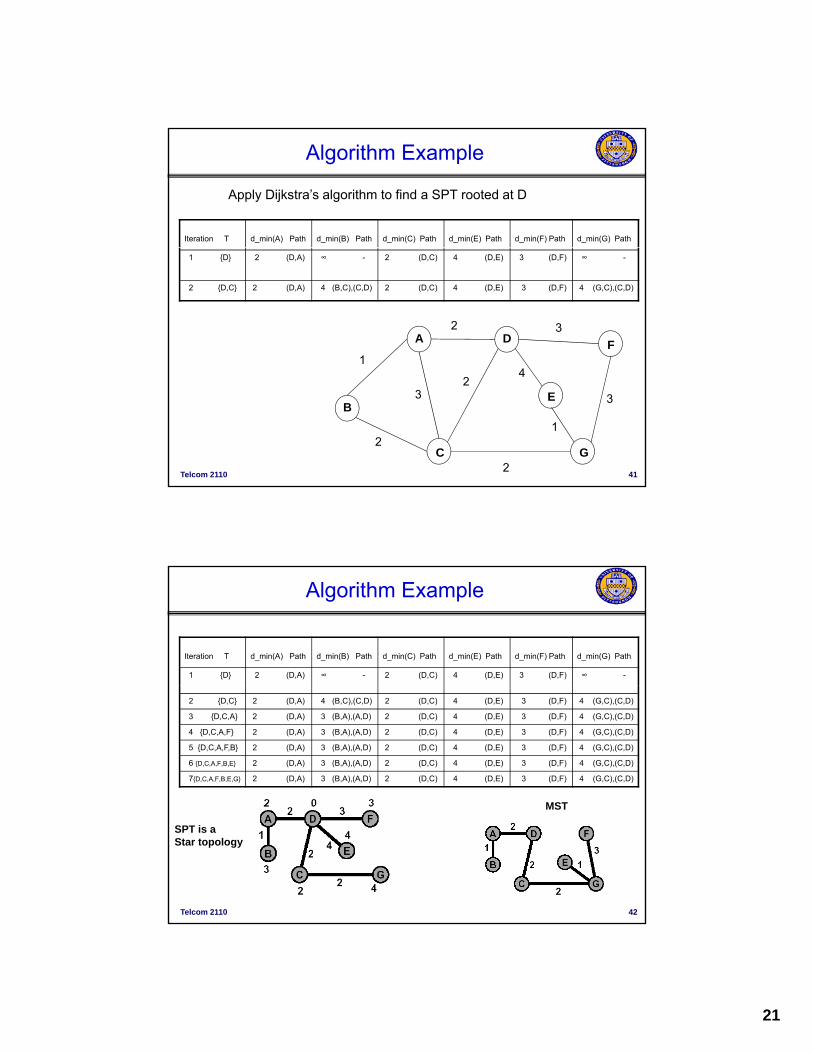
Shortest-Path Trees (SPT)
• Shortest PathGiven a weighted graph (G,W) and nodes n1 and n2, the shortest path from n to n is a path P such that the sum ofshortest path from n1 to n2 is a path P such that the sum of link weights along the path is a minimum.
• Shortest Path Tree– Given a weighted graph (G,W) and a node n1, a shortest – path tree
rooted at n1 is a tree T such that, for any other node n2 G, the path from n1 to n2 in the tree T is a shortest path between the nodes.
Pe
ew )(
Telcom 2110 38
• SPT vs. MST– SPT cost more, but will have lower link utilization and lower delay,
smaller average hop count
20
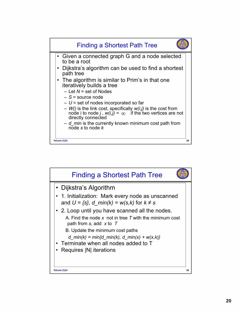
Finding a Shortest Path Tree
• Given a connected graph G and a node selected to be a root
• Dijkstra’s algorithm can be used to find a shortest path treepath tree
• The algorithm is similar to Prim’s in that one iteratively builds a tree– Let N = set of Nodes– S = source node– U = set of nodes incorporated so far– W() is the link cost specifically w(i j) is the cost from
Telcom 2110 39
– W() is the link cost, specifically w(i,j) is the cost from node i to node j , w(i,j) = if the two vertices are not directly connected
– d_min is the currently known minimum cost path from node s to node k
Finding a Shortest Path Tree
• Dijkstra’s Algorithm • 1. Initialization: Mark every node as unscanned
and U = {s} d min(k) = w(s k) for k ≠ sand U = {s}, d_min(k) = w(s,k) for k ≠ s
• 2. Loop until you have scanned all the nodes.A. Find the node x not in tree T with the minimum cost path from s, add x to T
B. Update the minimum cost paths
d min(k) = min{d min(k), d min(x) + w(x,k)}
Telcom 2110 40
d_min(k) min{d_min(k), d_min(x) w(x,k)}• Terminate when all nodes added to T• Requires |N| iterations
21
Apply Dijkstra’s algorithm to find a SPT rooted at D
P (Failure) = 10p2(1-p)3 + 10p3(1-p)2 +5p4(1-p) + p5
23
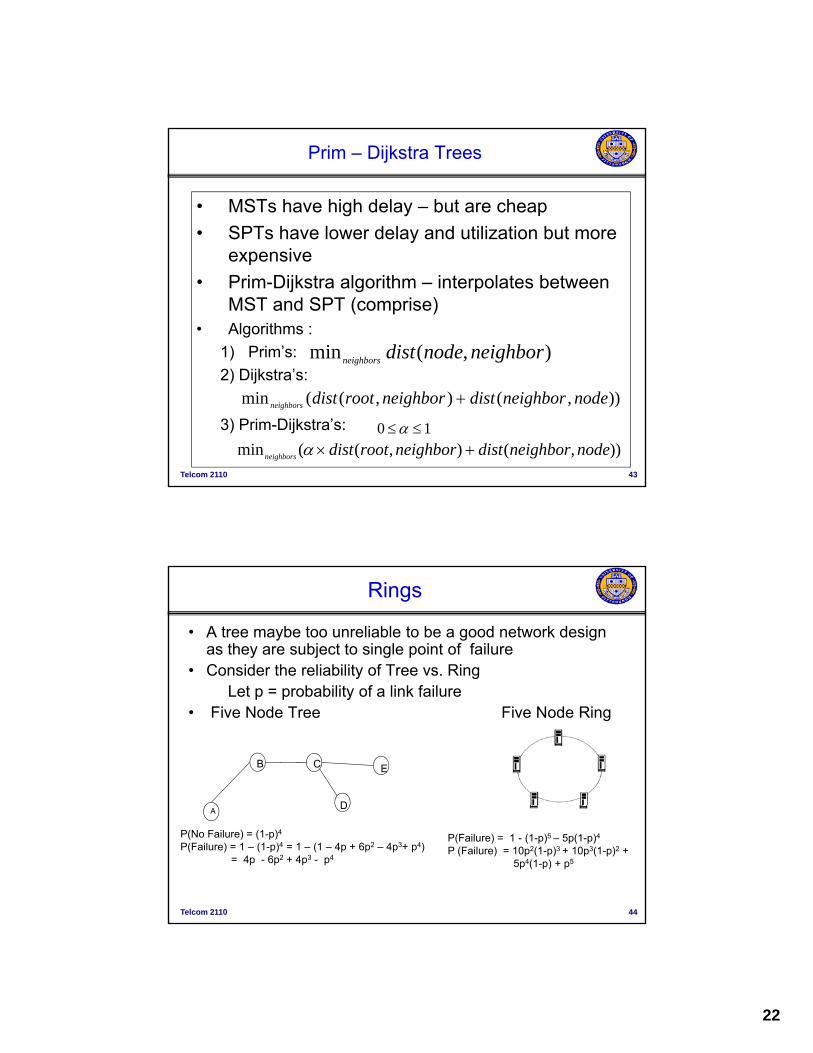
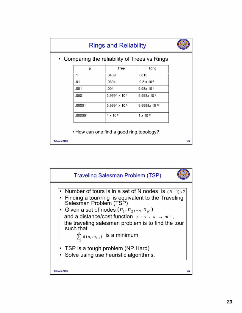
Rings and Reliability
• Comparing the reliability of Trees vs Rings
p Tree Ring
.1 .3439 .0815
.01 .0394 9.8 x 10⁻⁴
.001 .004 9.98x 10⁻⁶
.0001 3.9994 x 10⁻⁴ 9.998x 10⁻⁸
.00001 3.9994 x 10⁻⁵ 9.9998x 10⁻¹⁰
Telcom 2110 45
.000001 4 x 10⁻⁶ 1 x 10-11
• How can one find a good ring topology?
Traveling Salesman Problem (TSP)
• Number of tours is in a set of N nodes is• Finding a tour/ring is equivalent to the Traveling
Salesman Problem (TSP)
2/)!1( N
Salesman Problem (TSP)• Given a set of nodes
and a distance/cost function , the traveling salesman problem is to find the tour such that
is a minimum.
),...,,( 21 Nnnn NNd :
N
ii nnd 1 ),(
Telcom 2110 46
• TSP is a tough problem (NP Hard)• Solve using use heuristic algorithms.
i 1
24
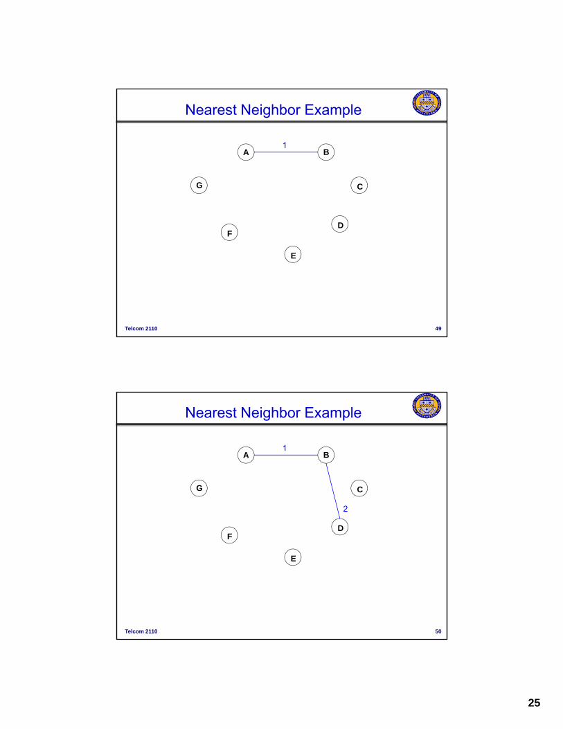
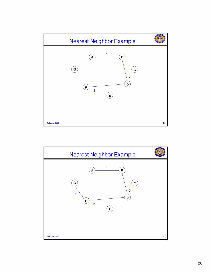
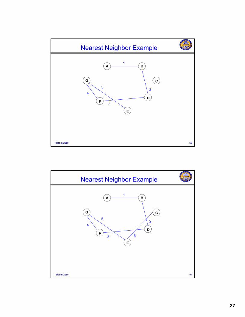
Nearest-neighbor Algorithm
1. Start at a node we call root and set current_node = root.
2. Loop until we have all the nodes in the tour.– Find the node closest (i.e., min cost or distance )
to the current_node that is not in the tour. We call this best_node.
– Create an edge between current_node and best_node.R t th t d t th b t d
Telcom 2110 47
– Reset the current_node to the best_node.
3. Finally create an edge between the last node and the root to complete the tour.
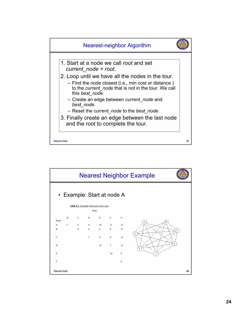
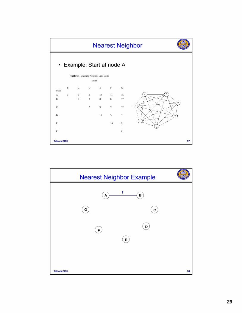
• Example: Start at node A
Nearest Neighbor Example
Table 6.1 Example Network Link Costs
Node
NodeB C D E F G
A 5 6 9 10 11 15
B 9 6 6 8 17
C 7 9 8 12
Telcom 2110 48
D 10 5 11
E 14 9
F 8
25
A B1
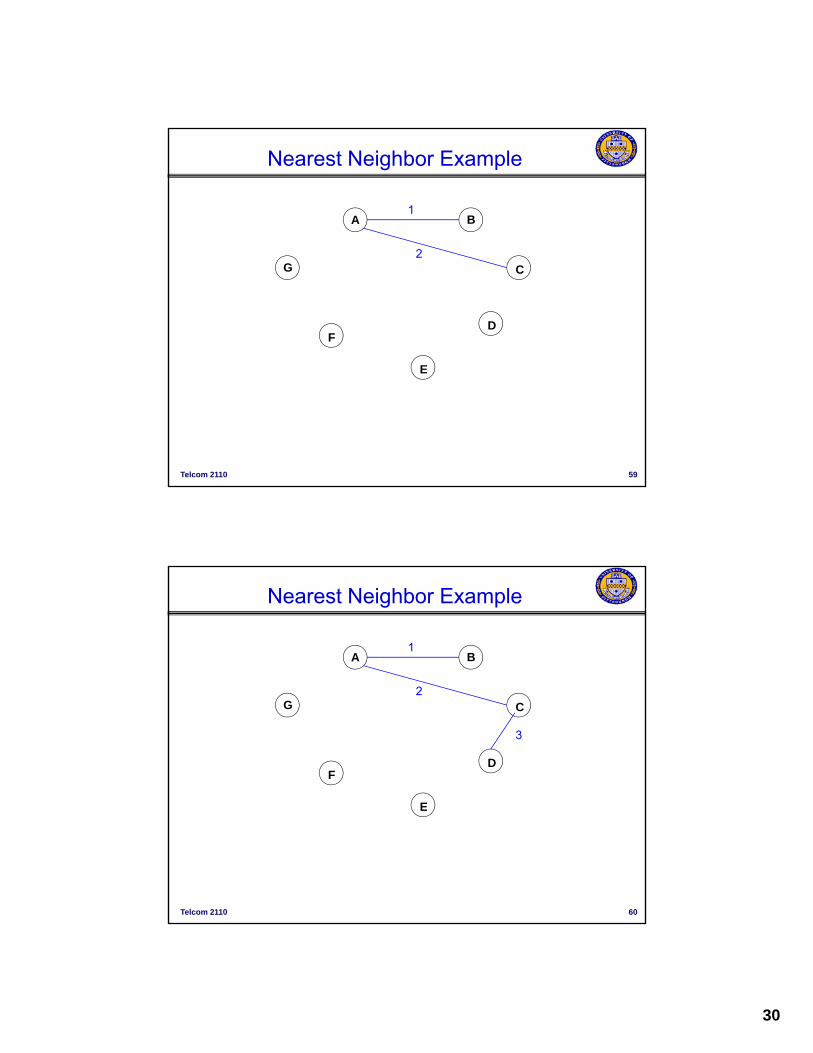
Nearest Neighbor Example
G
FD
C
E
Telcom 2110 49
E
A B1
Nearest Neighbor Example
G
FD
C
E
2
Telcom 2110 50
E
26
A B1
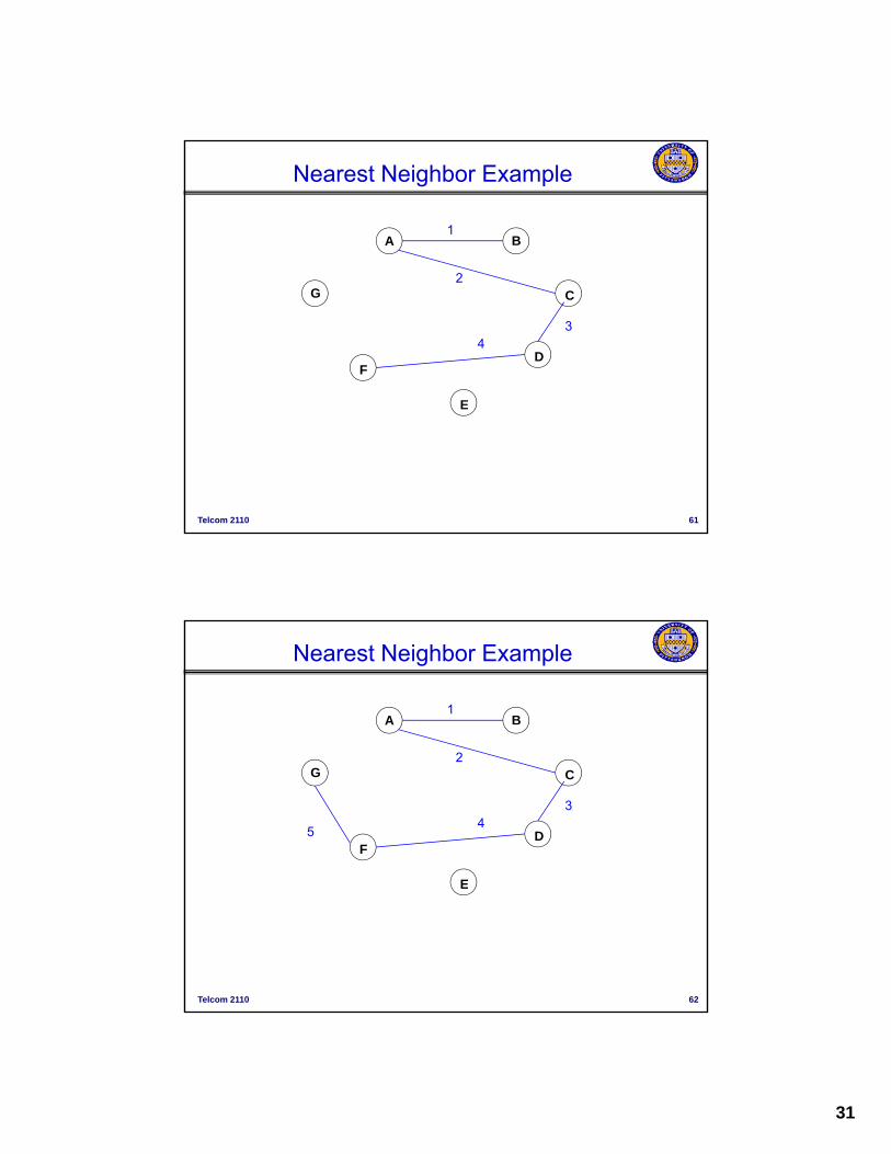
Nearest Neighbor Example
G
FD
C
E
2
3
Telcom 2110 51
E
A B1
Nearest Neighbor Example
G
FD
C
E
2
3
4
Telcom 2110 52
E
27
A B1
Nearest Neighbor Example
G
FD
C
E
2
3
4
5
Telcom 2110 53
E
A B1
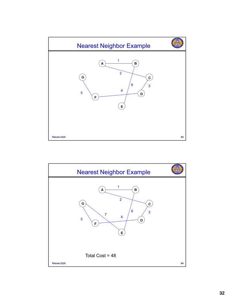
Nearest Neighbor Example
G
FD
C
E
2
3
4
5
6
Telcom 2110 54
E
28
A B1
Nearest Neighbor Example
G
FD
C
E
2
3
4
5
6
7
Telcom 2110 55
E
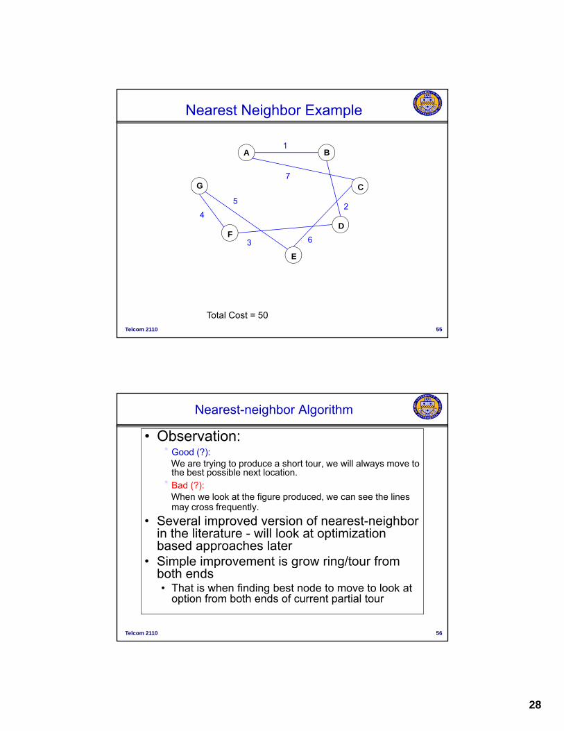
Total Cost = 50
Nearest-neighbor Algorithm
• Observation: * Good (?):
We are trying to produce a short tour, we will always move to the best possible next location.p
* Bad (?): When we look at the figure produced, we can see the lines may cross frequently.
• Several improved version of nearest-neighbor in the literature - will look at optimization based approaches laterSimple impro ement is gro ring/to r from
Telcom 2110 56
• Simple improvement is grow ring/tour from both ends • That is when finding best node to move to look at
option from both ends of current partial tour
29
Nearest Neighbor
• Example: Start at node A
Table 6.1 Example Network Link Costs
Node
NodeB C D E F G
A 5 6 9 10 11 15
B 9 8 8 8 17
C 7 9 7 12
Telcom 2110 57
D 10 5 11
E 14 9
F 8
A B1
Nearest Neighbor Example
G
FD
C
E
Telcom 2110 58
E
30
A B1
Nearest Neighbor Example
G
FD
C
E
2
Telcom 2110 59
E
A B1
Nearest Neighbor Example
G
FD
C
E
2
3
Telcom 2110 60
E
31
A B1
Nearest Neighbor Example
G
FD
C
E
2
34
Telcom 2110 61
E
A B1
Nearest Neighbor Example
G
FD
C
E
2
34
5
Telcom 2110 62
E
32
A B1
Nearest Neighbor Example
G
FD
C
E
2
34
5
6
Telcom 2110 63
E
A B1
Nearest Neighbor Example
G
FD
C
E
2
34
5
67
Telcom 2110 64
E
Total Cost = 48
33
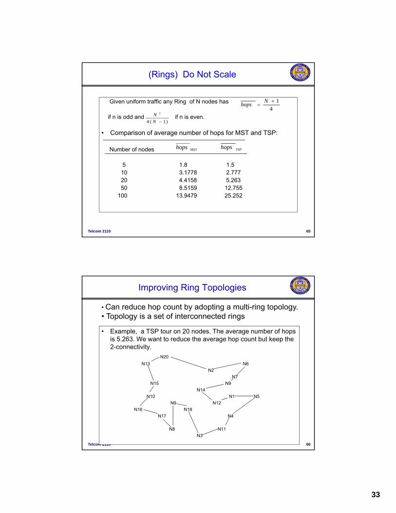
(Rings) Do Not Scale
Given uniform traffic any Ring of N nodes has
if n is odd and if n is even.
4
1
Nhops
)1(4
2
N
N
• Comparison of average number of hops for MST and TSP:
Number of nodes
5 1.8 1.510 3.1778 2.77720 4 4158 5 263
)1(4 N
MSThops TSPhops
Telcom 2110 65
20 4.4158 5.26350 8.5159 12.755
100 13.9479 25.252
Improving Ring Topologies
• Example, a TSP tour on 20 nodes. The average number of hops
• Can reduce hop count by adopting a multi-ring topology.• Topology is a set of interconnected rings
p , g pis 5.263. We want to reduce the average hop count but keep the 2-connectivity.
N20
N13 N6
N2
N7
N15 N9
N14
Telcom 2110 66
N10 N1 N5
N9 N12
N16 N18
N17 N4
N8 N11
N3
34
Divide and Conquer
• Use a Divide and Conquer approach
• Divide nodes into disjoint subset , construct ring for each subset, then join rings
• Example– Divide the 20 nodes into 2 “compact” clusters of 10 nodes each. Call
these clusters C1 and C2.
(We might divide the 20 nodes by ranges of their coordinates, for example, to create the 2 clusters.)
– Use the nearest-neighbor algorithm to design 2 TSP tours on each cluster.
S l t 1 C1 d 2 C2 t b th 2 d h th t th di t i
Telcom 2110 67
– Select v1 C1 and v2 C2 to be the 2 nodes such that the distance is the minimum.
– Now select v3 C1-v1 and v4 C2-v2 to be the 2 nodes such that the distance is the minimum.
– Add the edges (v1,v2), (v3,v4) to the design.
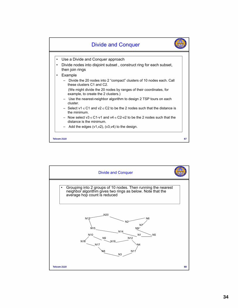
Divide and Conquer
• Grouping into 2 groups of 10 nodes. Then running the nearest neighbor algorithm gives two rings as below. Note that the average hop count is reduced
N20 N13 N6
N2 N7
N15 N9N14
N10 N1 N5
Telcom 2110 68
N10 N1 N5N9 N12
N16 N18N17 N4
N8 N11N3
35
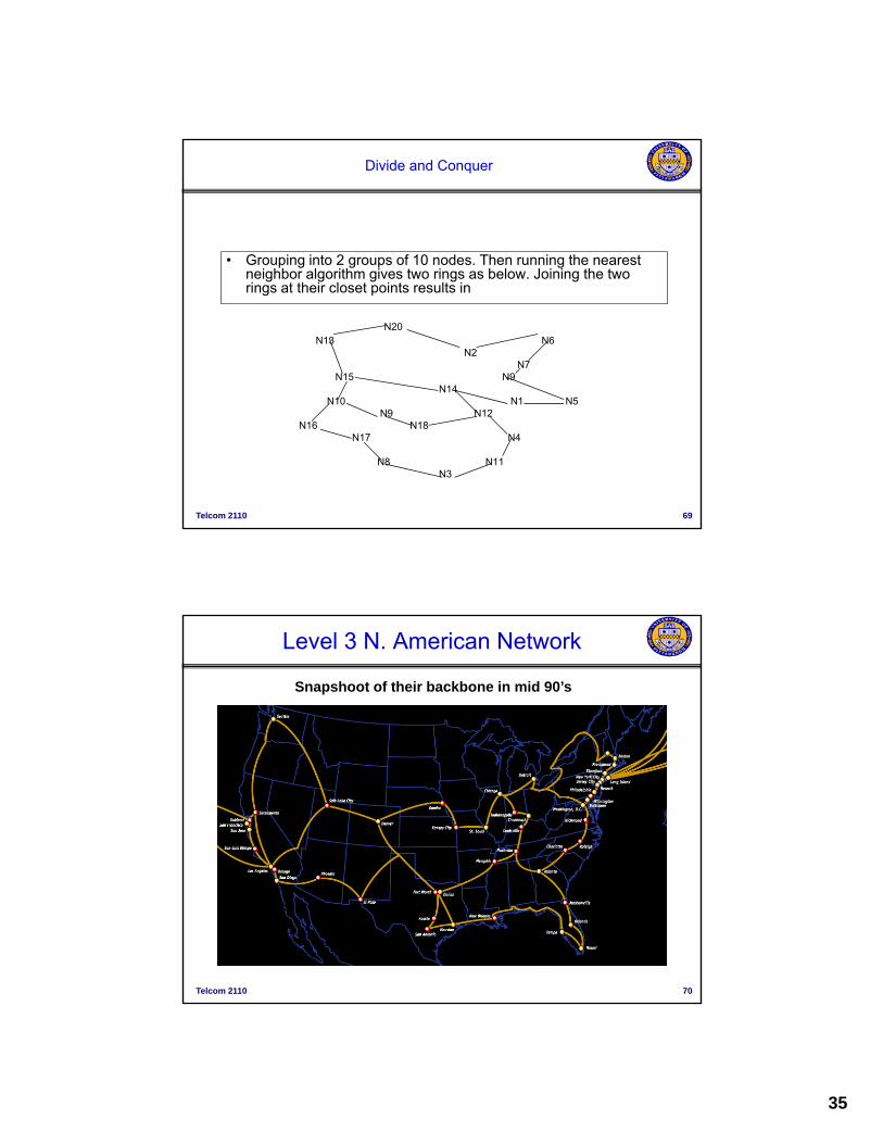
Divide and Conquer
• Grouping into 2 groups of 10 nodes. Then running the nearest i hb l ith i t i b l J i i th tneighbor algorithm gives two rings as below. Joining the two
rings at their closet points results in
N20 N13 N6
N2 N7
N15 N9N14
N10 N1 N5
Telcom 2110 69
N10 N1 N5N9 N12
N16 N18N17 N4
N8 N11N3
Level 3 N. American Network
Snapshoot of their backbone in mid 90’s
Telcom 2110 70
36
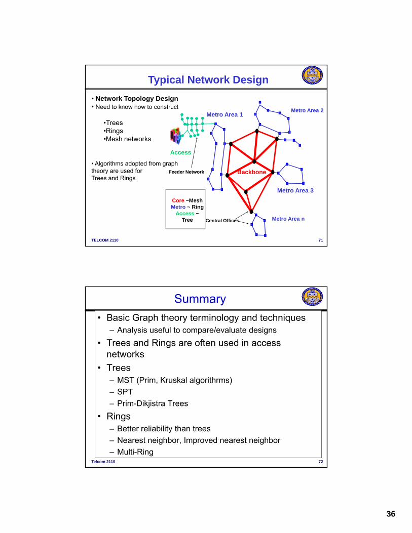
Typical Network Design
Metro Area 2Metro Area 1
• Network Topology Design• Need to know how to construct
•Trees
Backbone
Access
Feeder Network
•Rings•Mesh networks
• Algorithms adopted from graph theory are used for Trees and Rings
TELCOM 2110 71
Central Offices
Metro Area 3
Metro Area n
Core ~MeshMetro ~ Ring
Access ~ Tree
Summary
• Basic Graph theory terminology and techniques– Analysis useful to compare/evaluate designs
• Trees and Rings are often used in access gnetworks