Graphene: massless electrons in Graphene: massless electrons in flatland.flatland.

Work supported by:

University of Chile. Oct. 24th 2008

Enrico Rossi

Collaorators

Sankar Das Sarma

Shaffique Adam

Euyuong Hwang

Roman Lutchin

Close collaboration with experimental groups of:

CMTC, University of Maryland

Michael Fuhrer,University of Maryland

Jianhao ChenChau Jang

and

Ellen Williams,University of Maryland

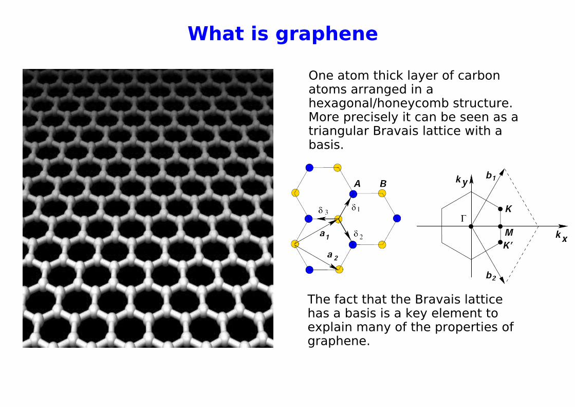
What is graphene

One atom thick layer of carbon atoms arranged in a hexagonal/honeycomb structure.More precisely it can be seen as a triangular Bravais lattice with a basis.

The fact that the Bravais lattice has a basis is a key element to explain many of the properties of graphene.

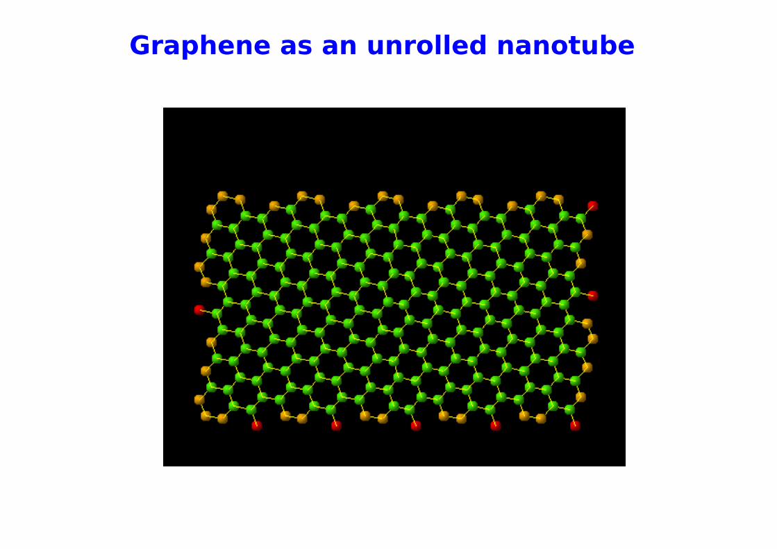
Graphene as an unrolled nanotube

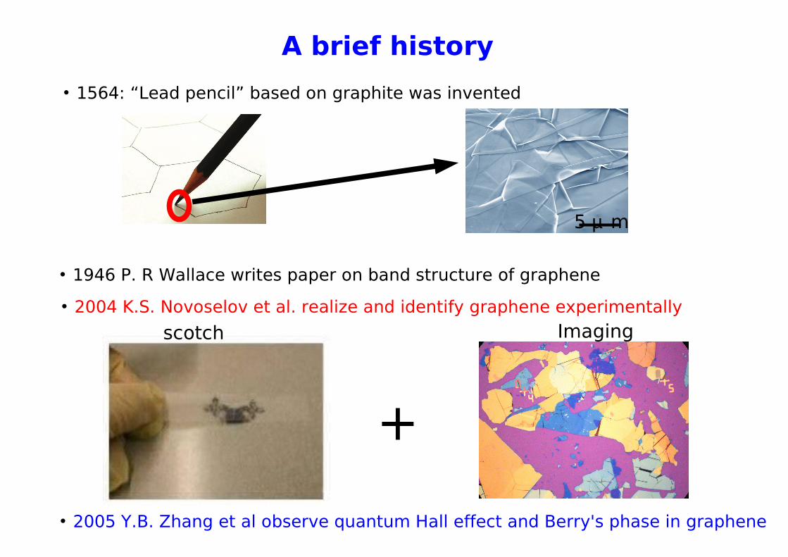
A brief history

1564: “Lead pencil” based on graphite was invented

5 µ m

1946 P. R Wallace writes paper on band structure of graphene

2004 K.S. Novoselov et al. realize and identify graphene experimentally

2005 Y.B. Zhang et al observe quantum Hall effect and Berry's phase in graphene

+

scotch Imaging

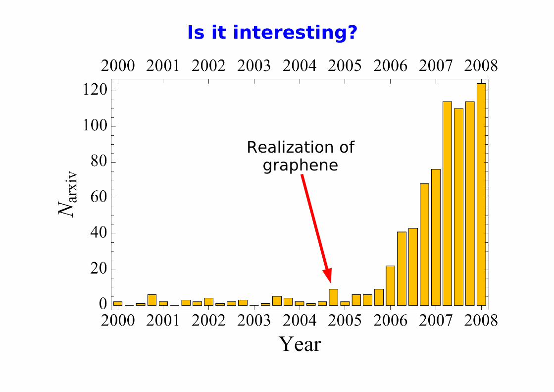
Is it interesting?

Realization ofgraphene

Why is graphene interesting: band structure

Each carbon atom as 4 bonds, 1 pz and 3 sp2 orbitals. The sp2 (s hybridized with p) leads to trigonal planar structure with formation of of a σ-bond between carbon atoms. The pz orbitals bind covalently with neighbors forming a half filled π-band

Graphene is truly 2D !

kx

ky

E

Tight binding model, P. R. Wallace (1947)

Bonding

Anti-Bonding`

Graphene has 2D Dirac cones

Dirac cones in graphene

From tight binding model we have that at the corners of the BZ the low energy Hamiltonian is:

kx' ky'

E

Chiral Massless Dirac Fermions

Electrons obey laws of 2D QED!

The Fermi velocity is ~ 1/300 the speed of light c. We have slow ultrarelativistic electrons.

QED with a pencil and some scotch!

Chirality

The sublattice symmetry implies that we have a conserved quantity:

chiralitydefined by the operator:

K’ Kbonding

anti-bonding

Courtesy of M. Fuhrer, University of Maryland

The Dirac point is protected by the conservation of

chirality.

Transport implication:

Back-scattering is suppressed.

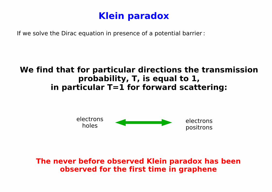
Klein paradox

If we solve the Dirac equation in presence of a potential barrier :

We find that for particular directions the transmission probability, T, is equal to 1,

in particular T=1 for forward scattering:

electronsholes

electronspositrons

The never before observed Klein paradox has been observed for the first time in graphene

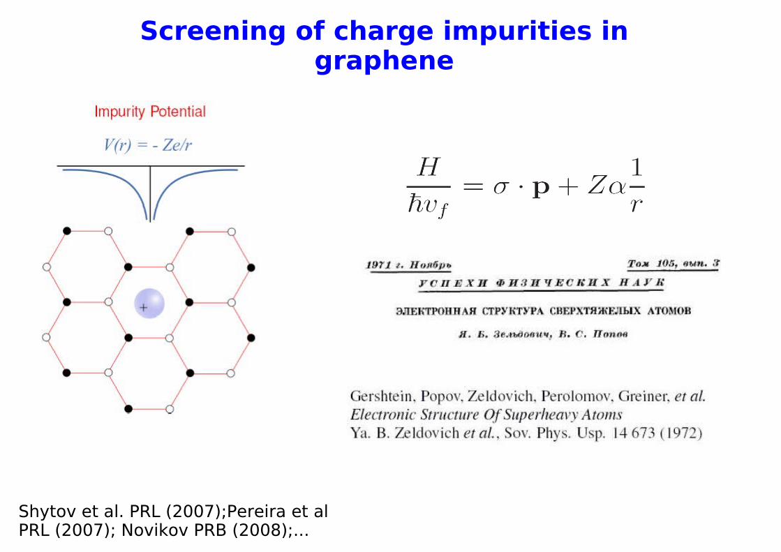
Screening of charge impurities in graphene

Shytov et al. PRL (2007);Pereira et al PRL (2007); Novikov PRB (2008);...

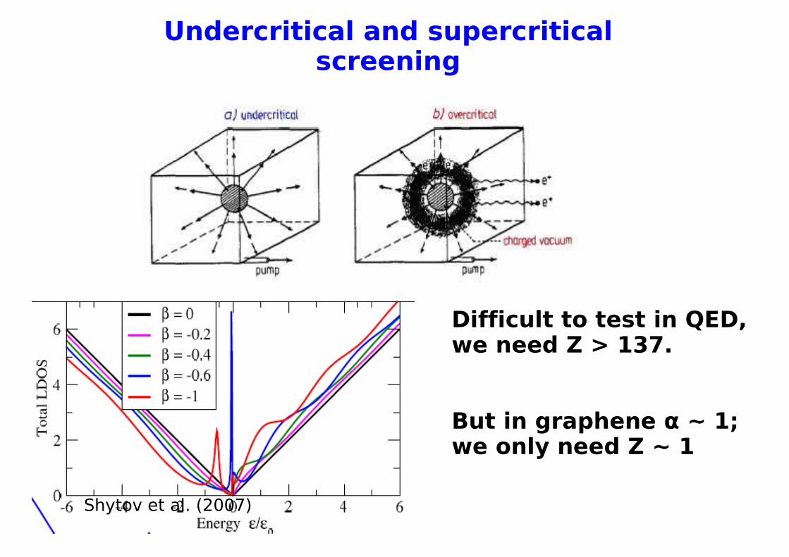
Undercritical and supercritical screening

Shytov et al. (2007)

Difficult to test in QED, we need Z > 137.

But in graphene α ~ 1;we only need Z ~ 1

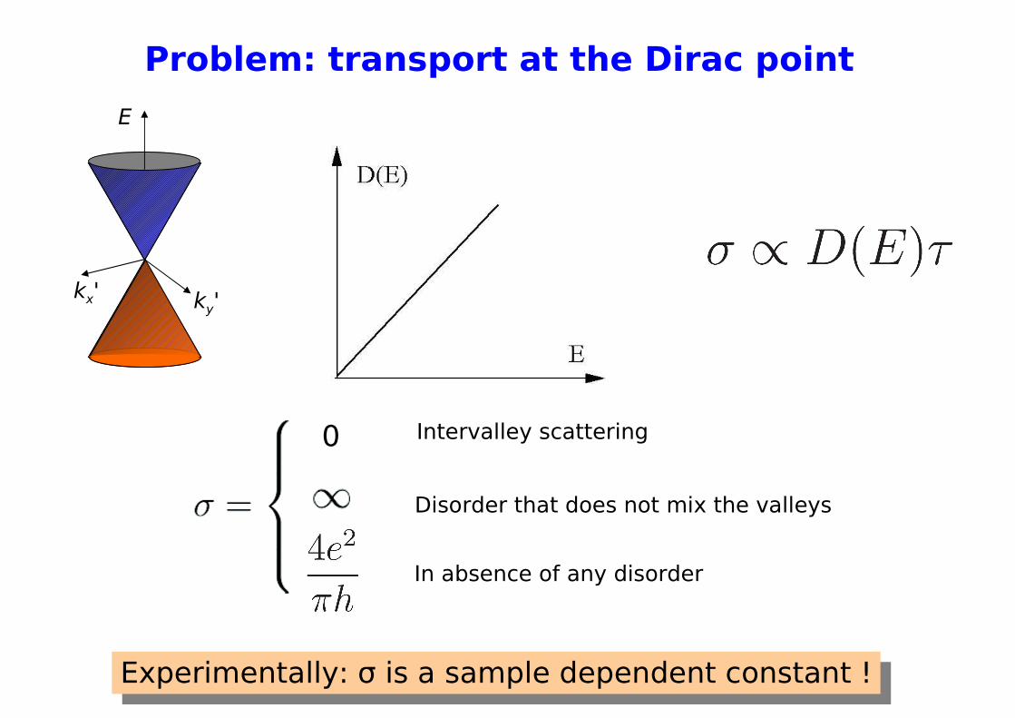
Problem: transport at the Dirac point

kx' ky'

E

0

In absence of any disorder

Disorder that does not mix the valleys

Intervalley scattering

Experimentally: σ is a sample dependent constant !

Effect of disorder

Scattering Shifts bottom of the band shift of Fermi energy

At the Dirac point disorder induces electron-hole puddles

Suggested theoretically :

E.H. Hwang, S. Adam, S. Das Sarma., PRL, 98, 186806 (2007).

Observed experimentally:

J. Martin et al., Nature Physics,4, 144 (2008)

System

Linear scaling region well explained by presence of random charged impurities

Graphene

Average distance of impuritiesfrom the graphene layer

Impurities

Substrate

Back-gate

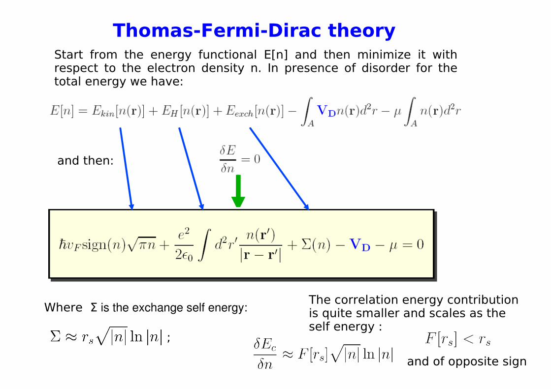
Thomas-Fermi-Dirac theory

and then:

Where Σ is the exchange self energy:

Start from the energy functional E[n] and then minimize it with respect to the electron density n. In presence of disorder for the total energy we have:

The correlation energy contribution is quite smaller and scales as the self energy :

;

and of opposite sign

Construction of disorder potential

We assume charge distribution with zero average. A nonzeroaverage it simply translates in a voltage gate off-set.

We assume the charge positions to be uncorrelated.

We then calculate C(q) using random number with Gaussian distribution and variance equal to impurity density.

Assuming the impurities to be in a layer at distance d we finallycalculate V

D

c

c

Dirac point: single disorder realization

We can see that many-body effects, exchange, tend to suppress the density fluctuations as it can be seen from the “histogram” plot of the density distribution.

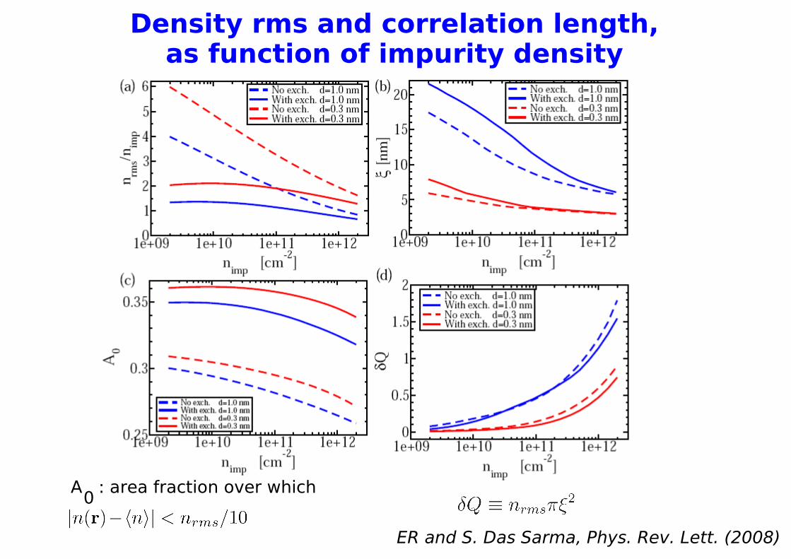
Density rms and correlation length,as function of impurity density

0A : area fraction over which

ER and S. Das Sarma, Phys. Rev. Lett. (2008)

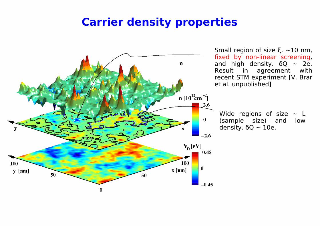
Small region of size ξ, ~10 nm, fixed by non-linear screening, and high density. δQ ~ 2e. Result in agreement with recent STM experiment [V. Brar et al. unpublished]

Wide regions of size ~ L (sample size) and low density. δQ ~ 10e.

Carrier density properties

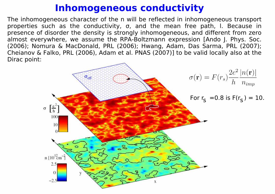
Inhomogeneous conductivity The inhomogeneous character of the n will be reflected in inhomogeneous transport properties such as the conductivity, σ, and the mean free path, l. Because in presence of disorder the density is strongly inhomogeneous, and different from zero almost everywhere, we assume the RPA-Boltzmann expression [Ando J. Phys. Soc. (2006); Nomura & MacDonald, PRL (2006); Hwang, Adam, Das Sarma, PRL (2007); Cheianov & Falko, PRL (2006), Adam et al. PNAS (2007)] to be valid locally also at the Dirac point:

For r =0.8 is F(r ) = 10.ss

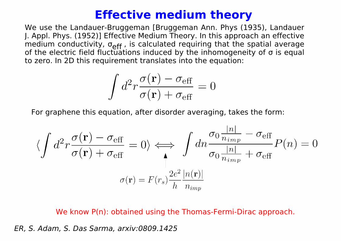
Effective medium theory We use the Landauer-Bruggeman [Bruggeman Ann. Phys (1935), Landauer J. Appl. Phys. (1952)] Effective Medium Theory. In this approach an effective medium conductivity, σ , is calculated requiring that the spatial average of the electric field fluctuations induced by the inhomogeneity of σ is equal to zero. In 2D this requirement translates into the equation:

eff

For graphene this equation, after disorder averaging, takes the form:

We know P(n): obtained using the Thomas-Fermi-Dirac approach.

ER, S. Adam, S. Das Sarma, arxiv:0809.1425

In general we have seen that ξ is ~10 nm, smaller than the typical l. However:

ξ characterizes small regions that are quite sparse and, in first approximation, we can assume their contribution to the conductivity to be small; Close to the Dirac point most of the sample is characterized by wide regions with small density. Because is ; in this regions l is quite smaller than the length scale over which n varies.

Effective medium theory: regime of validity

The Effective Medium Theory is valid when:

From Boltzmann-RPA result

a)

b) Resistive contribution due to boundaries between e-h puddles is small.,[Cheianov & Falko, PRB (2006); Cheianov et al, PRL (2007); Fogler et al. PRB (2008)].

This contribution becomes less important with the size of the e-h puddles.

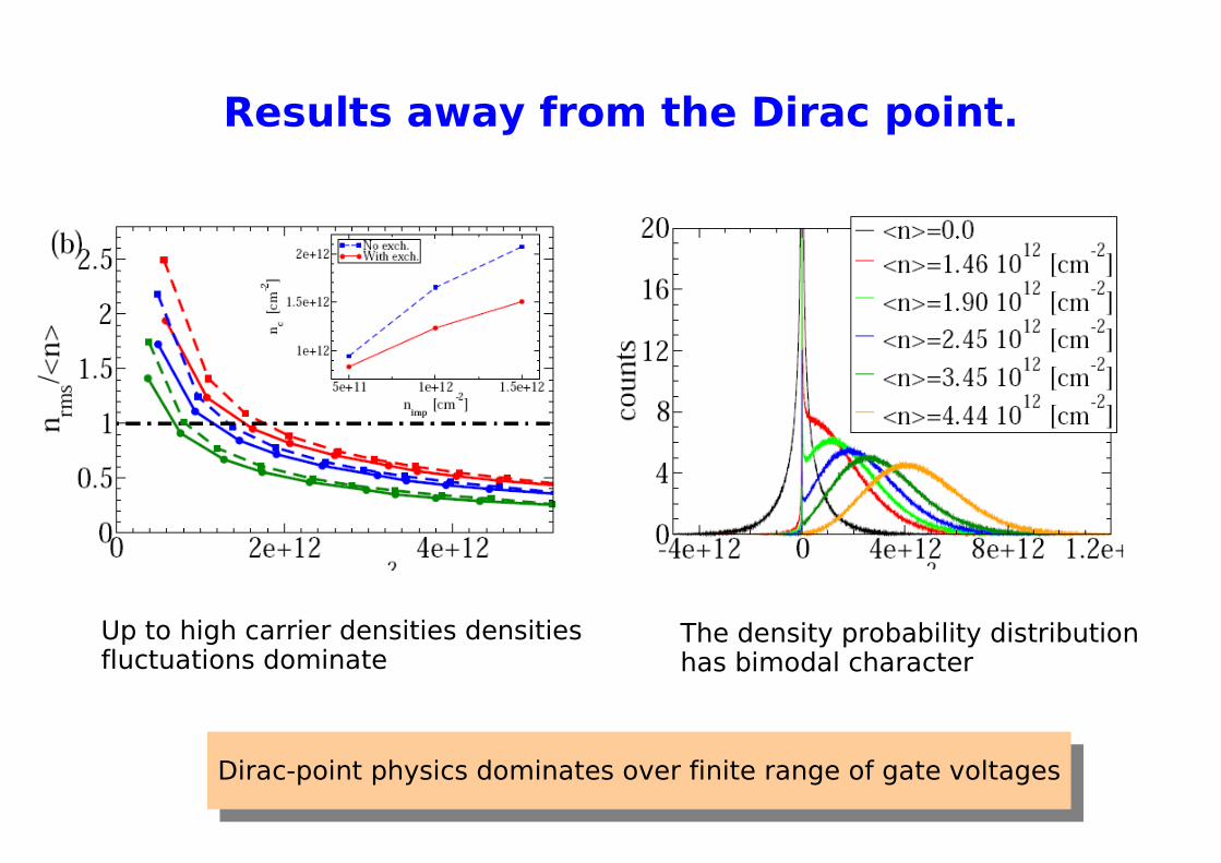
Up to high carrier densities densitiesfluctuations dominate

The density probability distribution has bimodal character

Dirac-point physics dominates over finite range of gate voltages

Results away from the Dirac point.

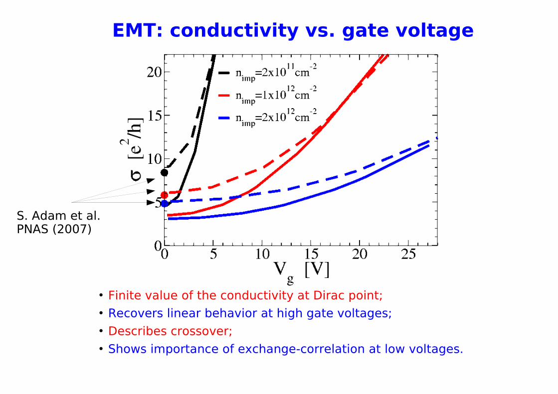
EMT: conductivity vs. gate voltage

Finite value of the conductivity at Dirac point; Recovers linear behavior at high gate voltages; Describes crossover; Shows importance of exchange-correlation at low voltages.

S. Adam et al.PNAS (2007)

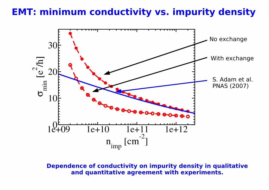
EMT: minimum conductivity vs. impurity density

Dependence of conductivity on impurity density in qualitativeand quantitative agreement with experiments.

No exchange

With exchange

S. Adam et al.PNAS (2007)

Tuning rs

C. Jang et al. PRL (2008)

Vacuum Ice

Graphene

How rs enters the theory rs affects the ground-state carrier distribution:

rs controls the scattering time:

S. Adam et al. PNAS (2008).E. Hwang et al. PRB (2008).

and therefore the local value of the conductivity

EMT: rs dependence of the minimum conductivity

Experiment: C. Jang et al PRL (2008)

Conclusions

Close to the Dirac-point, disorder induced density inhomogeneities are extremely important to understand graphene properties, especially transport.

We understand transport in current samples close to Dirac point;

Interactions not strong enough to cause long-range order but essential to understand transport close to the Dirac point;

Many things not covered and still largely unexplored: bilayers; graphene nanostructures, ...

Graphene is interesting.