Gravity Models of International Trade: Estimating the Elasticity of Distance with Finnish International Trade Flows. Master’s Thesis / Pro Gradu -tutkielma Veikko Rautala 181126 University of Eastern Finland / Itä-Suomen Yliopisto Economics / Kansantaloustiede Spring / Kevät 2015
Transcript
Gravity Models of International Trade:
Estimating the Elasticity of Distance with Finnish International Trade Flows.
Master’s Thesis / Pro Gradu -tutkielma
Veikko Rautala
181126
University of Eastern Finland / Itä-Suomen Yliopisto
Economics / Kansantaloustiede
Spring / Kevät 2015
Abstract
In this Master’s thesis a simple gravity model using Finnish bilateral trade flows is estimated. The
purpose of this paper is to estimate the coefficient of distance for Finnish exports/imports. We
examine three trade theories (Ricardian, Heckscher-Ohlin and monopolistic competition) to provide
theoretical background. Microeconomic foundations á la Bergeijk and von Brakman (2010) are
derived to attain a theory-driven empirical model. The model is estimated with random effects
estimator and spans the period of 2001-2012 and includes the 39 most important trading partners of
Finland. It is concluded that the elasticity of imports with respect to distance in case of Finish exports
and imports is close to the estimates found in the meta-analysis by Head and Mayer (2013).
Keywords: gravity – Finnish trade – random effects – distance – single country
Tiivistelmä
Tässä Pro Gradu –tutkielmassa mallinnetaan Suomen ulkomaankauppaa käyttämällä ns.
gravitaatiomallia. Tutkielman pääasiallisena tarkoituksena on määritellä etäisyyden vaikutus Suomen
ulkomaankauppaan. Työn teoreettisessa osassa esitellään kolmea ulkomaankaupan mallia
(Ricardolainen, Heckscher-Ohlin ja monopolistisen kilpailun malli). Mikroteoreettinen pohja
empiiriselle estimoinnille rakennetaan seuraten Bergeijk ja von Brakmanin (2010) esittämää
yleistystä. Metodina käytetään random effects –estimaattoria ja data käsittää aikavälin 2001-2012
vuositasolla ja sisältää 39 Suomen tärkeintä kauppakumppania. Tulokseksi saadaan, että Suomen
vientielastisuus suhteessa etäisyyteen myötäilee Head ja Mayerin (2013) meta-analyysissa saatuja
tuloksia.
Avainsanat: gravitaatio – Suomen ulkomaankauppa – random effects – etäisyys – maakohtainen
2.1. The Ricardian Model .............................................................................................................................. 5
2.2. The Heckscher-Ohlin Model ................................................................................................................ 11
2.2.1. The 2x2x2 Model........................................................................................................................... 11
2.2.2. Extensions and Criticism of the Simple H-O Model ..................................................................... 13
2.3. Models with Monopolistic Competition ............................................................................................... 15
2.4. Hybrid Models and Summary............................................................................................................... 19
3. The Gravity Model .................................................................................................................................. 23
3.1. Generalized Delivery of a Gravity Equation ........................................................................................ 26
3.2. Gravity Equation with a Single Exporter and/or Importer ................................................................... 29
4. Finland in the World Trade ..................................................................................................................... 31
5. The Empirical Model ............................................................................................................................... 37
6.1. Literature .............................................................................................................................................. 49
6.2. Finland as the Sole Exporter ................................................................................................................. 50
6.2.1 Main Export-model......................................................................................................................... 50
6.2.2. Auxiliary Export-model with added variable Price ....................................................................... 54
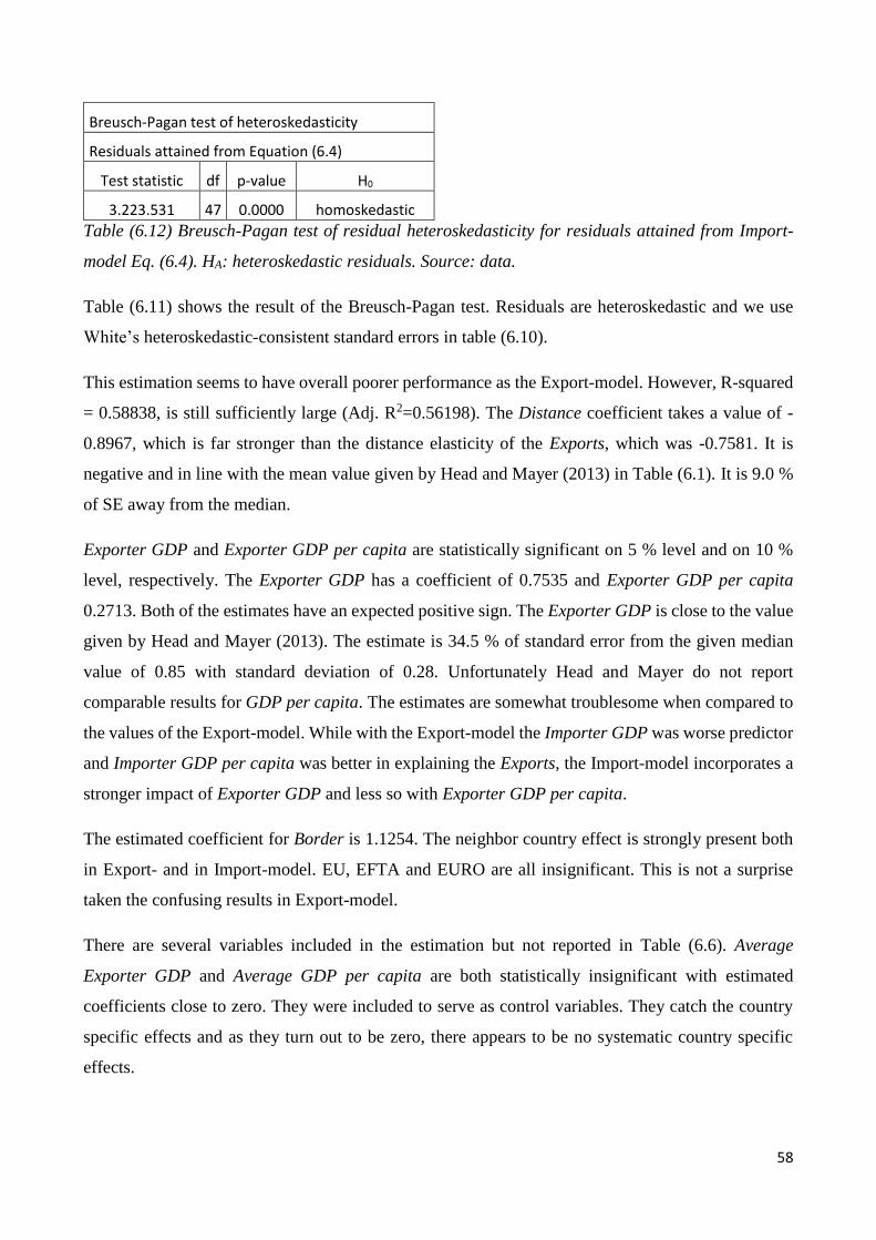
6.3. Finland as the Sole Importer ................................................................................................................. 57
6.3.1. Main Import-model........................................................................................................................ 57
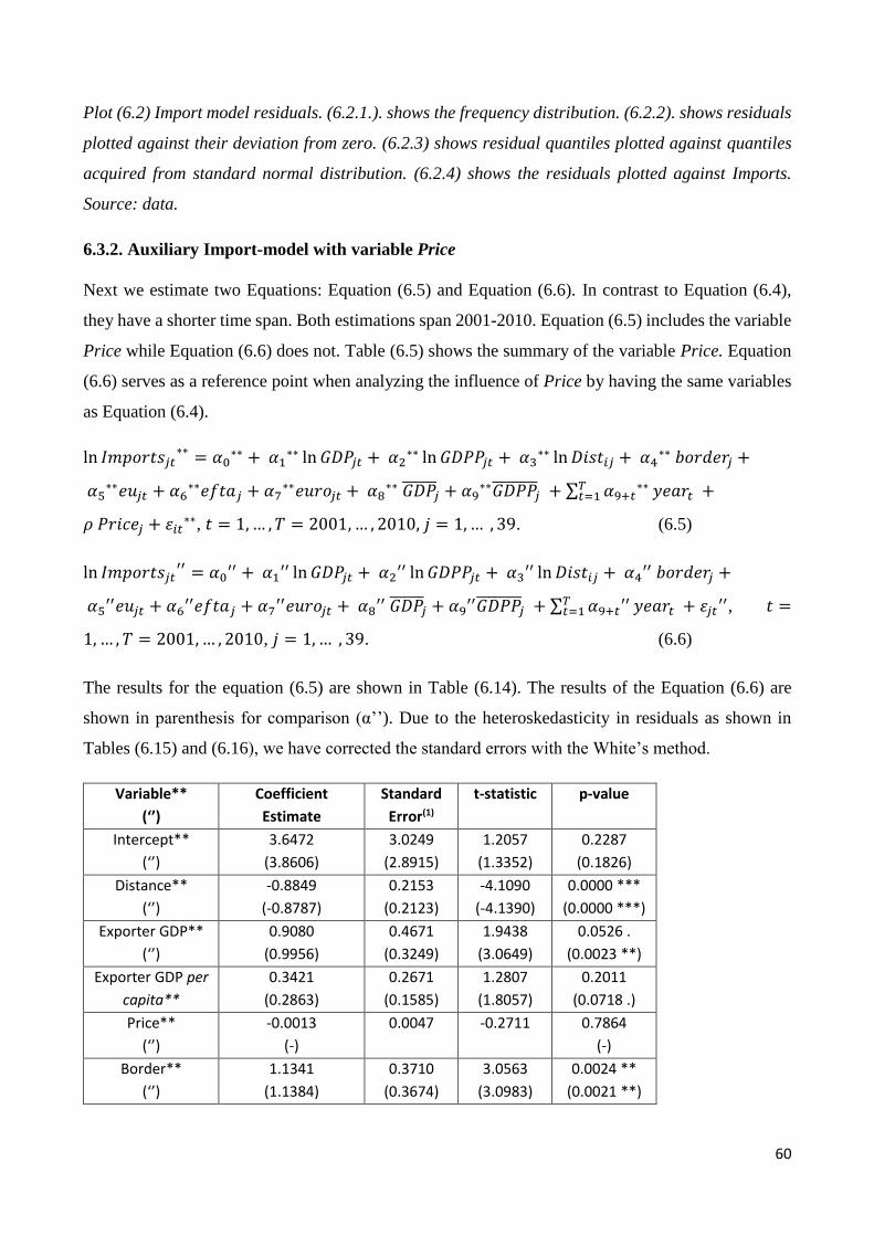
6.3.2. Auxiliary Import-model with variable Price ................................................................................. 60
7.3. A Word of Criticism ............................................................................................................................. 66
Appendix A.2. Fixed Effects, Random Effects and the Lagrange Multiplier Test .......................................... 78
2
1. Introduction
In this Master’s thesis we apply the so called gravity equation into Finnish international trade. The
purpose of this paper is to estimate some key parameters, which are commonly found in gravity
literature. The most important is distance, which directly relates the geographical distance of trading
partners with the occurrence of trade. We estimate a contemporary gravity model and give estimates
of the influence of distance to Finnish trade. We have chosen distance to be our key parameter,
because of its traditional role of estimating the trade costs between trading partners. Our other key
parameters include Gross national product, Gross national product per capita and contiguity.
During past few decades the gravity model has become the generally accepted workhorse for the
empirical research in international trade (Baier and Bergstrand 2002; Irwin and Eichengreen 1998).
Gravity models entered the field of economics already in the end of 19th century, but it took a long
time to gain popularity in empirical economics. Timbergen (1962) and Pöyhönen (1963) separately
introduced the gravity equation to trade. Since then, it has been used to estimate for example flows
of service offshoring, immigration or commuting. (Head and Mayer, 2013 Chapter. 2.4.)
The gravity model is named after Newtonian physics. The Newton’s law of universal gravitation
states that the bilateral gravitational force between two particles is positively related to the size of the
both particles and negatively related to the squared distance between the two particles. This equation
is then adjusted with the gravitational constant. Mathematically this takes the form:
𝐹 = 𝐺 𝑚1𝑚2
𝑑2 , (1.1)
where F is the gravitational force between two particles, m1 and m2 the respective masses of the
particles, d the distance between the centers of the masses, and G the gravitational constant. (Christie,
2002)
In international economics these masses of the Newtonian gravity equation are converted to economic
units. The particles in a gravity model of trade are economical areas, like countries or regions,
depending on the subject of research. The mass of such a particle is then the size of the economy in
this area. This is generally approximated by the gross domestic product (GDP) in the area. Changing
the respective variables in eq. (1) we have the classical gravity equation:
𝑀𝑖𝑗 = 𝐴 𝐺𝐷𝑃𝑖 𝐺𝐷𝑃𝑗
𝐷𝐼𝑆𝑇𝑖𝑗𝛼 , (1.2)
3
where Mij is the endogenous variable of interest. In this case it is the trade flow from country i to
country j. A is a constant, GDPi and GDPj are the Gross Domestic Product of the bilateral trading
partners and DISTij is the distance between the center of economic masses of the partner countries
(often distance between capitals). (Christie, 2002)
Attempts have been made to fit the gravity models to different pre-existing trade theories such as the
Ricardian model of trade, Heckscher-Ohlin model and models with monopolistic competition
(Deardorff, 1995; Evenett and Keller, 2002). Deardorff (1995) also noted that gravity equation is
easily adapted to any kind of trade theory. We visit the three listed trade theories in Section 2. The
trade theories are to serve as a theoretical background, however, we do not address the question of
fitting our empirical results to any particular trade theory. We discuss the role of gravity equation in
providing proof to pre-existing theories shortly in the end of Section 3.
The equation has gained more ground since its adaption to international economics. It has gained a
well-established microeconomic theory behind it. We follow van Bergeijk and Brakman (2010) and
introduce a general gravity model in Section 3. This is derived from a simple micro-economic theory.
We derive the model along the lines of monopolistic competition introduced in Section 2
We build the first gravity estimation exclusively of Finnish total trade. We mainly focus on the effect
of distance in Finnish context. The aim is to show how Finnish trade roughly follows the main stylized
facts on linking trade with distance in general. There exists no paper which has exclusively focused
on Finnish trade in the context of gravity that we are aware of1. Therefore this thesis simply aims to
bring the gravity equation to the discussions of Finnish trade and trade policy. However, we do not
aim to generate policy implications as a result of this paper. The policy implications which may be
generated shall be carefully discussed in Section 7.
In Section 3 we derive a theoretical gravity model along the lines of van Bergeijk and Brakman
(2010). We shortly discuss the composition of Finnish trade in Section 4. Along the overhaul, we try
to discuss the role of the trade theories introduced in Section 2 in explaining the direction of trade
from and to Finland. The overhaul is kept simple and short. In Section 5 we build an empirical model
based on the theoretical model in Section 3. We estimate this model in Section 6 with Section 7
discussing the results. As there does not exist another paper linking gravity with Finnish trade, we
1 The sole paper we found is a Master’s Thesis by Yingna Zhang, considering Finnish High Technology Exports, made in University of Helsinki/University College London in 2013.
4
use the meta-analysis by Head and Mayer (2013) and a paper by Fölvári (2006) as reference points
to anchor our results.
5
2. Theoretical Background
In this section we discuss three different theories found in international economics. They are
presented in a chronological order. The first one is the famous Ricardian approach to trade, which
assumes technological differences in determination of comparative advantage which in turn decides
the patterns of trade. The second approach is the so called Heckscher-Ohlin (H-O) model, where trade
patterns are determined due to differences in factor supplies. The third and last theory is one with
monopolistic competition (sometimes called by the authors, for example Helpman-Krugman-
Markusen model in Bergstrand (1989)) summarized by Krugman and Helpman (1985). After the
introduction of every theory we review the literature considering the shortcomings of the respective
theories. In the fourth subsection we review the attempts to merge the theories into a single model.
2.1. The Ricardian Model
The Ricardian model dates back to early nineteenth century, when British economist David Ricardo,
by whom the model is named after, first introduced it. The Ricardian model is based on the differences
in labor productivity. These differences give countries comparative advantage. Comparative
advantage is summarized by Krugman and Obstfeld (1996) as “A country has a comparative
advantage in producing a good if the opportunity cost of producing that good in terms of other goods
is lower in that country than it is in other countries.”2 (Krugman and Obstfeld 1996)
The Ricardian approach to international trade is found in every elementary textbook of international
economics. For reference here, we use the model descripted in the book International Economics –
Theory and Policy by Krugman and Obstfeld (1996). A basic Ricardian model is one with only one
factor of production, labor. An extension with more factors can be made and this is discussed later,
but for the simplicity, we first set up a one-factor model. We assume that a country can produce only
two goods, bread or cakes. Initially we look at a country which does not trade internationally.
We denote the amount of labor to produce one unit of bread by ab and the unit labor requirement to
produce one unit of cake by ac. We assume constant returns to scale so that ab and ac are constants
and labor requirements are independent of the quantity produced and do not change when more bread
or cakes are produced. Qb and Qc are the amounts of bread and cake that the country produces,
2 Opportunity cost means the lost production in all the other goods which could have been produced instead of the good which is actually produced. For example, if it is possible to produce only 10 breads or 5 cakes, a production of 10 breads has an opportunity cost of 5 cakes and vice versa.
6
respectively. As the total labor supply is L, the country faces a production possibility frontier defined
by the inequality:
𝑎𝑏 𝑄𝑏 + 𝑎𝑐 𝑄𝑐 ≤ 𝐿 (2.1)
We assume full employment. This implies that when all labor is employed, to produce one unit of
bread more, the country has to give up producing 1/ac units of cakes. Symmetrically, to produce one
unit of cakes more, the country has to give up 1/ab units of bread. These are the opportunity costs of
producing more bread or cakes. This trade-off can then be generalized by denoting the price of bread
in terms of cakes as ab/ac which is also the slope coefficient of the country’s production possibility
frontier.
Now we know what the country can produce, but to know what it actually produces, we have to turn
to the prices. We denote the price of bread by Pb and the price of cakes by Pc. Labor is mobile inside
a country and as the only factor of production it endows itself on the sector which pays the higher
wage. We assume zero-profits so that the wage (w) of a labor unit is the amount of output the unit
can produce, wb = Pb/ab and wc = Pc/ac, respectively. Now, if Pb/ab > Pc/ac, all labor will move onto
the bread sector to gain higher wages and if Pb/ab < Pc/ac, all labor will move onto cake sector. Only
when Pb/ab = Pc/ac or more conveniently Pb/Pc = ab/ac will both goods be produced. This means, that
the opportunity cost decides what a country will produce. A country will specialize in production of
a good, if its relative price is higher than its opportunity cost. In the absence of international trade,
the relative prices of goods equal their opportunity costs i.e. their relative unit labor requirements,
that is, Pb/Pc = ab/ac.
Now what happens when the country opens to international trade? Let us have a world with two
countries, Home and Foreign. They both have only one factor of production, labor, and they both
produce two products, bread and cakes, respectively. We denote the labor requirements of Home ab
and ac as above and the labor requirements of Foreign ab* and ac*, respectively. The labor
requirements can follow any pattern, but for the purpose of this model we make one arbitrary
assumption:
𝑎𝑏
𝑎𝑐 <
𝑎𝑏∗
𝑎𝑐∗ , (2.2)
which means that the ratio of labor needed to produce one unit of bread than one unit of cake is less
in Home than it is in Foreign. In other words, in Home, the relative productivity of bread is higher
than the relative productivity of cakes. Therefore Home has a comparative advantage in bread. This
7
comparative advantage depends on all the four labor requirements and is manifested in Equation
(2.2).3
By allowing the international trade we at the same time allow the prices to change across the countries.
If bread is cheaper in Home than in Foreign, Foreign will import bread from Home and export cakes
to Home. This leads to equalization in relative prices. We need a general equilibrium model to
describe what happens in the two-country world after it opens to international trade.
International equilibrium is reached in a point where relative demand and relative supply intersect.
The relative demand of bread is given by consumer preferences and substitution effect. Analyzing
the demand curve is not important for the purpose of the model, but we make an assumption of normal
downward sloping demand curve, where less bread is substituted for more cakes and vice versa.
However, the relative supply curve is more interesting. Figure (2.1)4 shows the market of bread with
relative supply and relative demand curves. The relative supply curve (RS) shows the total amount
of bread supplied. The moment the price drops below ab*/ac*, Foreign stops producing bread and the
same is true for Home, if the price drops below ab/ac. Only in the region of ab/ac < Pb/Pc < ab*/ac* both
countries produce bread.
The production is now affected by the demand curve. Take the relative demand curve RD in Figure
(2.1) as the first example. Relative demand and supply intersect in point A. In this case, Foreign
produces only cakes, because the price of bread is too low to be produced. Home produces only bread.
Both countries trade with each other to acquire both bread and cakes, but the comparative advantage
in bread by Home leads to the specialization in production. The price of the traded good in terms of
the other traded good changes and ends up somewhere in between the pre-trade autarky level.
Let us imagine the demand curve as in RD’ in Figure (2.1). The demand and supply now intersect in
point B. Foreign will still produce only cakes and Home will produce both bread and cakes. The
comparative advantage in bread in Home will still lead to the specialization in Foreign even though
Home now also produces some amount of cakes. This is caused by the low total relative demand of
bread compared to the above case, where equilibrium was reached in point A.
3 If we say that producing one unit of bread needs simply less labor in Home than in Foreign, that is ab < ab*, then Home has an absolute advantage in producing bread. However, this information is not enough to fully determine the patterns of trade. 4 Figure 2-3 in Krugman and Obstfeld (1996, chapter 2)
8
Figure (2.1). The RS curve shows relative supply for bread and RD curve shows relative demand for
bread in a two goods Ricardian model with an equilibrium in the intersection point A. Home produces
bread and Foreign produces cakes. RD’ is an augmented demand curve showing an equilibrium B in
the intersection point with RS. This leads Foreign to specialize in production of cakes, while Home
produces both bread and cakes. Source: Krugman and Obstfeld (1996).
We turn to analyze the gains of trade in this model. A way to see this is to understand Home producing
cakes through producing bread. Home could produce a unit of cakes by giving up production in bread
at a labor unit price of 1/ac. Alternatively, Home can produce an amount of bread of 1/ab and use this
to trade with Foreign at a price of Pb/Pc thus generating (1/ab)*(Pb/Pc) units of cakes with one labor
unit. This will be more or equal than cakes produced directly in Home as long as
1
𝑎𝑏 ×
𝑃𝑏
𝑃𝑐≤
1
𝑎𝑐, or put alternatively:
𝑃𝑏
𝑃𝑐 ≥
𝑎𝑏
𝑎𝑐. (2.3)
This equation holds in the international markets as we just derived it above. In an equilibrium where
both Home and Foreign specialize (point A), the world market price is Pb/Pc > ab/ac. As the same is
true for the Foreign with bread, we can declare that both countries are better off or at least the same
as in autarky after the introduction to international trade and there exists gains from trade. Opening
9
the economy to international trade leads to specialization of production and clearly defines the pattern
of trade flows between countries.
To make the model more realistic, a multitude of goods and factors may be added along with
transportation costs, tariffs and non-traded goods5. However, these added variables do not change the
basic result of the simplistic one-factor, two-goods model. Countries specialize to produce goods with
which they have a comparative advantage.
Deardorff discusses about the aspects of the Ricardian model in several papers (1995), (2004) and
(2005). In his 2004 paper, Deardorff points out how transportation costs may severely affect the trade
flows when they are high. Comparative advantage is distorted by country-pair specific advantages,
which rise from geographical proximity and cultural similarities driving down transportation costs,
which outset the productivity effects.
In the 2005 paper Deardorff notes that Ricardian model in the two-country or in two-goods form can
be educating, but unrealistic. A more realistic approach, allowing both multitude of goods and
multitude of countries is, however, hard to analyze. Some partial results can be delivered, but not as
strong predictions as the original two goods, two countries model. The constant returns to scale
assumption of the Ricardian models is also hard to comply with. Better working model of marginal
opportunity costs has been developed by Haberler (1930), but this no more implies a uniquely defined
comparative advantage.
Leamer and Levinsohn (1995) state that although there exists little or no empirical support to simple
Ricardian models, they help to give insight to the importance of technology in economic isolation.
They mark how hard it is to convert Ricardian models to empirically testable form. Empirically, they
state, there are three topics which could be empirically relevant. First, the gains from trade should be
testable. However, they also note that trading in the broader economic sense is one of the key
assumptions of economics and should not need testing. Secondly, they point that terms of trade in
this kind of models are bounded to differences in labor productivity, which should be testable. They
conclude that a one factor model is a “mathematical toy” without any meaning in the real world.
Thirdly, and perhaps the most importantly, Ricardian models bound exports to comparative cost
(dis)advantage. This is much too strong prediction to be found in the real world.
Allowing sector specific factors of production, we have an approach called Ricardo-Viner model.
However, by allowing factors to be mobile over sectors, this practically produces H-O model in a
5 See, for example Dornbusch et al (1976).
10
long run. (Leamer and Levinsohn, 1995) Therefore we do not proceed to analyze the Ricardo-Viner
model separately in this paper, while H-O model is discussed in the next subsection.
In spite of the criticism by Leamer and Levinsohn (1995), Eaton and Kortum (2002) built a model
with parameters relating to absolute advantage, comparative advantage and geographic barriers. They
estimated the model using bilateral data from 19 OECD countries and used it to address questions
about gains from trade, the role of spreading technology through trade and the effects of trade barrier
reductions. This work neglects the earlier claims that Ricardian model might be too theoretical to
apply in empirical works.
One of the recent papers, which build on the Ricardian model based on the paper of Eaton and Kortum
(2002), is the one presented by Costinot, Donaldson and Komunjer (2011). They seek to improve the
theoretical foundations and quantify the comparative advantage. They build a traditional Ricardian
model with multitude of goods, labor as the only factor of production, labor immobility, perfectly
competed markets, ice-berg transportation costs6 and Cobb-Douglas7 consumer preferences. The
ultimate goal was to study the relationship between observed trade levels and observed labor
productivity. Their labor productivity depends on two variables, one called fundamental productivity,
which catches the effects within a country across sectors and another which catches intra-industry
heterogeneity.
The observed productivity and fundamental productivity differ because some countries do not
produce at all those products in which they have comparative disadvantage. Their improvements to
the model are present when estimating the coefficient for fundamental productivity. Final estimation
is made by Instrumental Variable techniques. Results are robust and show that labor productivity can
be used as an estimator for trade flows and that the Ricardian approach is theoretically well-grounded.
They also show that gains from trade exist. (Costinot et al, 2011)
The Ricardian model catches the importance of comparative advantage, which is widely accepted in
the international trade theory. The Ricardian model can hardly be used to explain all the international
trade flows and it has been in downshift for a long period of time. In spite of this, the model has an
6The notation ice-berg transportation cost was coined by Samuelson (1954). It means that the transportation costs are compared to an ice-berg and some of the transported commodities simply ‘melt’ during the transportation. This means, that of every shipment Q, sent from point A to point B, only an amount of (1-t)Q arrives at point B. t is a transportation cost proportional to the Q and t takes a value 0<t<1. (Kurmanalieva (2006)) 7 Cobb-Douglas production function normally takes the form of Y=KαLβ. In the case of consumer preferences, the utility function for a consumer to maximize in a two good world takes the form of U=XαYβ. (Cobb and Douglas 1928)
11
advantage over its later counterparts in explaining international trade by the differences in labor
productivity, i.e. technological differences.
2.2. The Heckscher-Ohlin Model
The so called Heckscher-Ohlin model, also called the Factor Proportions Theory of International
Trade, is based on the writings of Hecksher (1919) and Ohlin (1933). This theory has been the
backbone of trade theories until recently (Leamer and Levinsohn, 1995). The most general result of
H-O model is that countries export goods which are produced with the most relatively abundant
factors in the country and import goods which use factors relatively scarce in the importing country.
We present the model here in its simplest form, which means that we have a model of two goods, two
factors and two countries.
2.2.1. The 2x2x2 Model
A typical H-O model consists of two factors of production which usually are capital (K) and labor
(L). Output also consists of two goods, for example, machinery (M) and food (F). We assume the
production of machinery to require lots of capital and the production of food to require relatively
more labor. This relativity is measured as the capital-labor (K/L) ratio of the respective industries.
Hence, machinery is capital-intensive sector and food is labor-intensive sector, or 𝐾𝑀
𝐿𝑀>
𝐾𝐹
𝐿𝐹. As the
intensiveness is measured in capital-labor ratio, a sector cannot be both labor- and capital-intensive.
If we denote the price of the capital as r and the price of the labor as w, the optimal rate of capital-
labor used in an industry will depend on the relative price of factors, w/r. (Krugman and Obstfeld,
1997, ch. 4)
We denote the price of machinery as PM and the price of food as PF. There is one-to-one relationship
between the factor prices and the prices of output. If the economy produces both goods and does not
trade internationally, it means that PM/PF = w/r. This follows the reasoning developed in the previous
section about the Ricardian model. In other words, the price of machinery will equal the factor price
ratio. This further means that capital-labor ratio of producing machinery and food must be KM/LM
and KF/LF, respectively. If the price of machinery now rises relatively to food, it will decrease the w/r
ratio of the production. This effect of output prices to factor prices is known as Stolper-Samuelson
theorem and it states that if output prices of a good rises, the price of a factor which is used intensively
in producing the good will rise. Because capital is now relatively more expensive, this will increase
the usage of labor in production increasing the KM/LM and KF/LF ratios, respectively. (Krugman and
Obstfeld, 1997, ch. 4)
12
Last condition needed to determine the equilibrium allocation of resources in this model is full
employment in both factors of production which we assume together with an assumption that the
country produces both goods.
What happens now if the availability of the other factor rises? If the availability of capital now
increases, both the production of machinery and food may expand. However, the expansion is biased
towards the production of machinery. This is generally known as the Rybczynski theorem (Leamer
and Levinsohn, 1995). Increase in the availability of capital increases the production of machinery
and decreases the production of food proportionally and vice versa. (Krugman and Obstfeld, 1997,
ch. 4).
To turn to the case of international trade, we have to make further assumptions. Usually made
assumptions include having only two countries (the last ‘2’ in ‘2x2x2 model), Home and Foreign.
Secondly, demand for the products is identical in both countries and they have the same production
technology. The only difference between the two countries is that they have different amounts of both
resources. We assume that Home has a higher labor to capital ratio than foreign, that is, L/K > L*/K*8.
Hence, Home is labor-abundant and Foreign is capital-abundant. (Krugman and Obstfeld, 1997, ch.
4)
Now, because of its labor-abundance, Home will tend to produce more food compared to Foreign and
Foreign tends to produce more machinery compared to Home. When Home and Foreign trade with
each other, Home (Foreign) will export (import) food and import (export) machinery. The relative
prices will converge. The relative price of machinery will increase in Home and decrease in Foreign,
thus generating a new world price which is in between the autarky prices of Home and Foreign.
(Krugman and Obstfeld, 1997, ch. 4)
The result is a main implication of the H-O model and generally known as the Heckscher-Ohlin
theorem. Countries well-endowed in a factor tend to produce and export products which use the
abundant factor intensively. In a similar fashion, countries scarce on a factor tend to import products
which require the scarce factor intensively in production. (Krugman and Obstfeld, 1997, ch. 4)
On the other hand, the convergence of the output prices leads to a convergence in factor prices. This
is generally known as the Factor Price Equalization theorem (FPE). The H-O model predicts that
with time the factor prices converge all the way until the relative prices are equal in both countries.
8 This is only an arbitrary assumption for the purpose of the model.
13
However, this FPE theorem is a controversial issue, because empirical results show that the factor
prices do not generally equalize between trading countries. We will come back to this issue below.
These four theorems listed in italics above are the main results of H-O model: The Heckscher-Ohlin
theorem, the Stolper-Samuelson theorem, the Rybczynski theorem and the FPE theorem.
2.2.2. Extensions and Criticism of the Simple H-O Model
A logical improvement to the model is to allow multiple goods and multiple factors of production.
This is known as Heckscher-Ohlin-Vanek (H-O-V) model. (Leamer, 1995)
Factor content studies which started with Leontief (1953) have produces mixed results. Factor content
studies aim to confirm or refute the H-O model. They search for patterns in actual correlations
between factor intensities in exports and imports compared to the abundance of the same factors in
the exporting/importing economy. Leontief’s paper in 1953 introduced an anomaly in H-O model.
Leontief descripted how US economy tends to export labor intensive products and import capital
intensive products. However, as Leontief noted, US economy is by any definition a capital abundant
economy. This finding controversies the H-O model which clearly states that capital abundant
countries export capital intensive products. This controversy was named after the author and is well
known as Leontief paradox. (Leamer and Levinsohn, 1995)
Leamer (1980) produced a paper in which he explains the Leontief paradox as a simple
misspecification by Leontief. Leontief compared the gross values of imports and exports, when a
correct measure, according to Leamer, would have been net values. Leamer finds out that the
Leontief’s paradox disappears, when net imports and exports are compared to capital-labor ratios of
US consumption. Hence, USA which exported in 1947 both labor and capital intensive goods in net
values, acts according to H-O-V model.
Bowen, Leamer and Sveikauskaus (1986) presented a multi-country, multi-factor and multi-goods
model, i.e. an H-O-V model. They dismiss many earlier papers by blaming them to be insufficiently
specified or that the estimated coefficients are falsely interpreted. They build a robust framework to
estimate a few different models.
However, mixed results follow. They do not find evidence for straight linkage between factor
abundance and country’s exports, as the H-O-V model suggests. This controversy is explained by two
things. First, they assume similar production technology for every country, which follows from the
theoretical assumption of factor price equalization. The results clearly dismiss this assumption and
14
suggest different factor endowment in different countries. Second, differences in regressions for
different factors and different countries implies, that significant measurement errors exist in
measuring both trade and national factor supply data. (Bowen, Leamer and Sveikauskaus (1986))
Leamer (1995) updates his earlier papers considering H-O model. In the introduction he writes in two
instances:
“Facts casually and not so casually collected seem to be adding up to a convincing case against the HO model.”
And:
“Yet the HO model remains very much alive and well, residing happily and prominently in every textbook on international economics written by authors fond of the artistic diagrams and simple, remarkable theorems associated with the HO viewpoint. (…).These authors understand that data analysis may hit the HO model so hard that it hollers ‘false,’ and that theorist may pin the model so firmly to the mat that it squeals ‘impressed,’ but the authors have not heard nor do they imagine ever to hear, the HO model scream ‘useless.’“
Leamer (1995) follows the literature in deriving a theoretical framework of H-O model. He then
proceeds to explain the evolvement of trade in four countries: Germany, USA, Japan and Sweden.
He divides trade to eleven different categories. He shows that factor supplies and net exports are
closely linked in some sectors, like machinery and chemicals. However, he also discovers that most
of the net exports of manufactures are hard to fully explain with factor supplies.
Leamer (1995) points to two theorems which seem to be the most troubling when considering the H-
O model. These are the Stolper-Samuelson theorem and the FPE theorem9. These two theorems link
factor supplies with income distribution and they have a dramatic influence when combined to
migration and global trade liberalization. Leamer points out how dramatic changes are to be expected
in low skill labor wages if these two theorems are true. According to FPE, low skill labor prices
should decline in the rich countries and increase in low income countries. However, he also points
two factors working against this force. First, a liberalization of trade should increase the global GDP
leading to an increase of the average wage everywhere. Second, a simple H-O model does not take
into account the different levels of human capital endowed in production. Another force against FPE
is technological differences.
9 Leamer hypothesizes that the name “Factor Price Equalization” is very misleading, because it only describes a setting in which the factor prices should equalize without actually telling anything about the process behind it.
15
2.3. Models with Monopolistic Competition
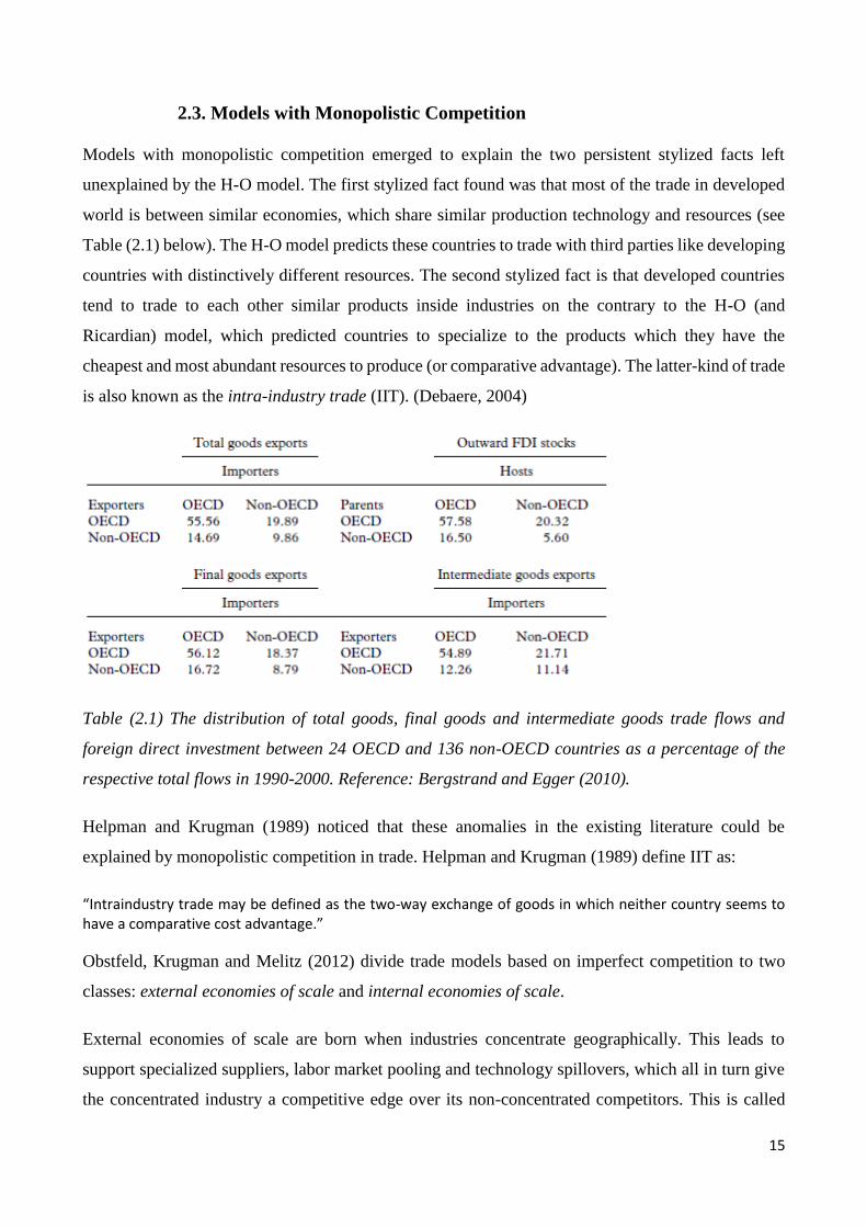
Models with monopolistic competition emerged to explain the two persistent stylized facts left
unexplained by the H-O model. The first stylized fact found was that most of the trade in developed
world is between similar economies, which share similar production technology and resources (see
Table (2.1) below). The H-O model predicts these countries to trade with third parties like developing
countries with distinctively different resources. The second stylized fact is that developed countries
tend to trade to each other similar products inside industries on the contrary to the H-O (and
Ricardian) model, which predicted countries to specialize to the products which they have the
cheapest and most abundant resources to produce (or comparative advantage). The latter-kind of trade
is also known as the intra-industry trade (IIT). (Debaere, 2004)
Table (2.1) The distribution of total goods, final goods and intermediate goods trade flows and
foreign direct investment between 24 OECD and 136 non-OECD countries as a percentage of the
respective total flows in 1990-2000. Reference: Bergstrand and Egger (2010).
Helpman and Krugman (1989) noticed that these anomalies in the existing literature could be
explained by monopolistic competition in trade. Helpman and Krugman (1989) define IIT as:
“Intraindustry trade may be defined as the two-way exchange of goods in which neither country seems to have a comparative cost advantage.”
Obstfeld, Krugman and Melitz (2012) divide trade models based on imperfect competition to two
classes: external economies of scale and internal economies of scale.
External economies of scale are born when industries concentrate geographically. This leads to
support specialized suppliers, labor market pooling and technology spillovers, which all in turn give
the concentrated industry a competitive edge over its non-concentrated competitors. This is called
16
external economies of scale, because the economies of scale are subject to the whole concentrated
industry instead of single firms. On the contrary, this kind of concentrated industry is often formed
by small competitive firms. The study concerned with the geographical concentration of industries is
called the Economic Geography10.
The latter case is the internal economies of scale. In this kind of models the industries face increasing
returns to scale in the company level. This lets the industries to concentrate on the hands of few
companies often creating an oligopoly. These firms then act as price-setters as opposed to the price-
takers of the perfect competition models. The oligopolies have market power. A certain form of
internal economies of scale is the case of monopolistic competition. In monopolistic competition each
company differentiates their product slightly compared to their competitors’ similar products. This
way the company has limited monopoly power that makes it independent of competitor’s price
decisions. The company acts like a monopoly even though in reality it faces competition. In this
section we will build on the assumptions of monopolistic competition, as it has grown to be popular
among trade theories during the past decades. (Obstfeld, Krugman and Melitz, 2012)
As stated above in the previous section, the H-O model predicts countries to export different products
with each other, thus leading to inter-industry trade – trade between different industries. However, an
increasing share of world trade is intra-industry trade (Krugman 1995), which the H-O models do not
take into account. Instead of dismissing the H-O theory, the monopolistic competition models have
risen next to the H-O models.
A basic model with monopolistic competition assumes that firms or countries differentiate their
products in such a way that they are not perfect substitutes for each other. This is done because each
product faces increased returns to scale. However, consumers love variety with Dixit-Stiglitz11 -
preferences. Free entry to markets allows the price to be competed down to marginal costs. This
10 The subject of Economic Geography has a far reaching literature on its own, which we shall not review here as it is beyond the scope of the paper. 11 Dxit Stiglitz preferences take the form of representative consumer maximizing his utility function U(C) where consumption, C, is given by the function:
𝐶 = (∫ 𝑐𝑖𝛼 𝑑𝑖)
1
𝛼, over a continuum of goods, i = 1,…,N. A consumer maximizes his utility by maximizing a function:
∫ 𝑐𝑖𝛼 𝑑𝑖 subject to a constraint:
∫ 𝑝𝑖 𝑐𝑖 𝑑𝑖 ≤ 𝑌 where Y is income denoted by a numeraeire, ci is the consumption of good i, pi is price of the good i and the integral is taken over all the goods i, i = 1,…,N. The purpose of this kind of function is to create a utility function, where an extra An extra good always increases consumer’s utility. Hence, consumers love variety. Note that this result depends on the assumption that 0 < α < 1 and the elasticity of substitution σ > 1. (Dixit and Stiglitz, 1977)
17
section introduces a basic model of monopolistic competition with IRS based on the Helpman and
Krugman (1989) which in turn is practically based on the model presented by Dixit and Stiglitz
(1977).
An economy is able to produce a large variety of symmetrical goods which face consumer demand
based on the utility function:
𝑈 = [ ∑ 𝐷𝑖𝛼𝑛
𝑖=1 ]1
𝛼, 0 < α < 1 (2.4)
where Di is the consumption of i:th good and n is the number of available varieties. This utility
function incorporates the elasticity of substitution of any given products, that is, σ = 1/(1-α) > 1. The
demand for any product i is given by
𝐷𝑖 = 𝐷 [𝑝𝑖
𝑃]−𝜎, (2.5)
where
𝐷 = ∑ [𝐷𝑖𝛼]
1
𝛼𝑛𝑖=1 , (2.6)
𝑃 = ∑ [𝑝𝑖
𝛼
𝛼−1]𝛼−1
𝛼𝑛𝑖=1 . (2.7)
pi denotes the price of i:th product and P is basically a price index. D is an index of total consumption.
A firm which produces a good i and is small enough to be unable to affect price level P faces demand
curve with elasticity of σ.
On the production side, only one factor of production is assumed. To produce a unit of (any) good xi,
a labor amount of f(xi) is needed. There are economies of scale so that average output per worker is
increased when output is increased (𝜕 𝑓(𝑥𝑖)
𝜕𝑥𝑖> 0). Because of economies of scale there is imperfect
competition. The number of products is unlimited or sufficiently big, which assures that there is no
reason for two firms to produce the same product. This lets us say that there is only one product per
firm.
Firms act as monopolies and set their prices such that marginal revenue equals marginal costs:
𝑤 𝑓′(𝑥𝑖) = 𝑝𝑖 𝜎−1
𝜎, or
𝑝𝑖
𝑤= 𝑓′(𝑥𝑖)
𝜎
𝜎−1, (2.8)
18
where w is the wage rate of the employed labor. Because there is asymptotically no entry restrictions,
the extra profits are competed away. This means that price is equal to average cost:
𝑝𝑖
𝑤=
𝑓′(𝑥𝑖)
𝑥𝑖, (2.9)
The equilibrium is given by (2.8) and (2.9) as the pricing rule and the zero-profit condition equal:
𝑓′(𝑥𝑖) 𝜎
𝜎−1=
𝑓(𝑥𝑖)
𝑥𝑖. (2.10)
The equilibrium gives output per firm and sets prices compared to wages. The number of goods
produced, n, is given in equation with full employment:
𝑛 =𝐿
𝑓(𝑥). (2.11)
Now we assume that there are two countries, Home and Foreign. Both have identical demands based
on the utility function in Eq. (2.4). Both countries can trade with each other and there exists (for
simplicity) no transportation costs. What happens to the production? Nothing. Both countries produce
a variety of products, Home n and Foreign n*. Consumer love for variety in both countries makes
them demand certain amount of goods from the other country. This produces IIT. As Krugman and
Obstfeld (1996) point out, underlying the model with economics of scale is the idea that a country’s
production is constrained by the size of its market. Taking part in international trade increases market
size and loosens this constraint. There are gains from trade in this model simply because a consumer
has access to greater variety of goods with trade than in autarky.
The model does not tell us which goods are produced. However, this is not important as all the goods
are identical. It also does not tell us which goods are produced in which country as it is totally arbitrary
in this model. This is a model with imperfect competition but it develops a way to analyze intra-
industry trade as two countries with similar products trade with each other.
Paul Krugman addressed the theoretical background of the monopolistic competition in several his
papers. In a chapter written in 199512, he establishes a three-sector model in which one of the sectors
has external economies of scale. He shows how the scale economies lead to concentration of the
respective industry in one country. He then proceeds to show that this leads to intra-industry trade
alongside the prevailing inter-industry trade and that there exists gains from trade.
12 Handbook of international Economics, vol. III, chapter 24, pp. 1243-1277, Edited by K. Grossman and K. Rogoff, 1995.
19
Melitz (2002) builds on the monopolistic competition by making a model in which he explains
industry heterogeneity by limited entry to export markets. In this model only the most profitable firms
can enter the export markets, because the entry preserves a fixed entry-cost. Firms enter and exit the
market simultaneously and reallocate resources inside the industry. Exposure to trade leads the
industry to gain efficiency through reallocation, and leaves the welfare enhancing effects of trade
untouched.
Helpman (1987) generates a model to test three hypotheses of the monopolistic competition model.
His theoretical foundation to the model is given by Helpman and Krugman (1985, ch. 8, which we
have also consulted in our derivations above). The testable hypotheses are listed as: 1) the larger the
similarity in factor composition, the larger is the intra-industry trade. 2) The more similar the factor
composition between countries becomes over time, the larger the intra-industry trade between the
countries. 3) The changes in relative country sizes explain the rise in trade-income ratio. All the
hypotheses are found to be consistent with the data.
Hummels and Levinsohn (1995) note that the empirical works considering the monopolistic
competition models are relatively scarce. Rather, the monopolistic competition models have led
empirical models to two directions: the models which combine inter-industry H-O trade and intra-
industry monopolistic competition trade, and the gravity models of trade. We will consider the hybrid
models in the next subsection, and give a more extended explanation of the gravity model in the
Section 3.
2.4. Hybrid Models and Summary
All of the three theories which we have presented so far approach the international trade from a
slightly different perspective. All of them give some insight to the forces working behind the
determination of trade. However, none of them is conclusively superior to the others. As the theories
give different insights of the same prevailing phenomenon, a further question rises of why the models
could not be combined to a single hybrid model to attain better results.
Cieslik (2007) points out that indeed further research is needed around this topic, namely in
combining the Heckscher-Ohlin and the monopolistic competition models. Cieslik notes that only a
few papers have addressed this problem: Helpman (1987), Hummels and Levinsohn (1995), Evenett
and Keller (2002) and Debaere (2005), respectively.
Hummels and Levinsohn (1995) reconsider the model presented by Helpman (1987). They discuss
the plausibility of the results and test Helpman’s results with their enhanced model. Like Helpman,
20
they build two models. The first one predicts trade flows by assuming all trade to be intra-industrial,
in other words, subject to monopolistic competition. The first model fits the data (only OECD
countries) remarkably well. It fits the data well even with very heterogeneous non-OECD countries,
which raises a question about the correct specification of the model. They discard this first model as
implausible with too strict assumptions.
The second model assumes only a fraction of the trade to be intra-industrial13. Mixed results follow.
Most of the intra-industry trade turns out to be a result of country specific effects. They declare the
model to be indecisive. Generally they conclude the paper noting that further research is needed and
they are pessimistic of the monopolistic competition in explaining the trade. It should be noted, that
the model in this paper is closely related to gravity models, thought missing some important elements
such as distance and multilateral resistance (we come back to these issues in the Section 3). (Hummels
and Levinsohn, 1995)
Debaere (2004) contradicts the results delivered by Hummels and Levinsohn (1995). He shows how
the model of Hummels and Levinsohn is falsely specified. He builds his own model to show that the
Helpmans (1995) original paper, in which the paper by Hummels and Levinsohn is based, is
consistent with OECD countries but cannot rightfully be said to be consistent with the non-OECD
data presented by Hummels and Levinsohn. However, in spite of this, Debaere does not provide any
further additives to the discussion about the choice between H-O and monopolistic competition
models.
Evenett and Keller (2002) continue to study the effect of specialization in the H-O, monopolistic
competition and mixed models. They point out, how specialized the economies are both in pure H-O
model and monopolistic competition models. Their study of the data shows that a pure H-O model or
a pure monopolistic competition model finds little evidence, respectively. However, a model, mixing
together both models to a one with imperfect specialization among the bilaterally trading countries,
has mixed results. It predicts that when the intra-industry trade is high among the bilateral trading
partners, the model correctly predicts more product differentiation. On the other hand, the link to the
H-O is more tenuous. However, the predictions of a model with imperfect specialization solely due
13 Evenett and Keller (2002) as well as Helpman (1979), and Hummels and Levinsohn (1995) use the Grubel-Lloyd index to index the intra-industry composition of trade. The index is provided by Evenett and Keller as:
𝐺𝐿𝑖𝑗 = 1 − (∑ |𝑀𝑔𝑖𝑗
− 𝑀𝑔𝑗𝑖
|𝑔 ∑ |𝑀𝑔𝑖𝑗
+ 𝑀𝑔𝑗𝑖
|)𝑔⁄ 0 ≤ 𝐺𝐿 ≤ 1,
where g = 1…G is an index for industry and Mij exports from country i to country j. On extremes, when GL = 0, there is no intra-industry trade, and when GL = 1 all the trade is in intra-industry. (Grubel and Lloyd 1971)
21
to differences in factor endowments finds support in the data. These confusing results lead the authors
to conclude, that both theories predict different components of the same dataset.
All the above discussed models mobilize a predecessor of a gravity model. They all have equations,
where the influence of certain parameters to bilateral trade flows between pairs of countries is
estimated. This is an important similarity between these models and the traditional gravity equation.
However, they do not include to their equations distance or any kind of trade cost function which are
essential variables in the gravity literature. What we see here, is that gravity equation can be modified
to address different empirical problems. In this case it was used to address the question of the correct
composition of trade.
We have seen how Ricardian and H-O both consider the comparative advantage of a country as the
source of trade. Ricardian employs technological differences – labor productivity – as the main
determinant in what a country exports and imports. H-O basically does the same, but with resources
as the source of comparative advantage. Incorporating Ricardian labor productivity to H-O should
not be impossible. Monopolistic competition adds to this mix and allows one to understand trade in
intermediates and in highly differentiated goods. In summary, all the theories explain a side of the
whole picture.
As gravity model is more an empirical approach to trade than a new trade theory, these three theories
serve a lesson when estimating a model. This means that we will not use the gravity equation to prove
the precluding theories of international trade, but rather to address the very same empirical problems
that have been presented in the context of the trade theories. Deardorff (1995) addressed the problem
of fitting gravity modeling with pre-existing trade theories and concludes:
“The lesson from all this is twofold, I think. First, it is not all that difficult to justify even simple forms of the
gravity equation from standard trade theories. Second, because the gravity model appears to characterize a
large class of models, its use for empirical tests of any of them is suspect.”
The theories give us a reason to add variables in the gravity model depending on the testable
hypothesis. The gravity equation provides but a framework, and does not itself prove anything. To
test for example the importance of technology or the resource base of an economy, one adds variables
to gravity accordingly.
In the next section we derive the gravity model from microeconomic theory. We remind that there
are multiple ways to arrive to a gravity-like equation and therefore our way is not exclusive of others.
Then later on this paper, in Sections 5 and 6, we show how a gravity model may be estimated with
22
contemporary techniques and which results may be derived using it. However, before we proceed to
construct our model, we consider the composition of Finnish economy and specially its trade in the
Section 4, because the estimations carried in later sections focus on Finnish trade.
23
3. The Gravity Model
Baier and Bergstrand (2007) give three reasons for the success of the gravity model in the past three
decades. First, formal economic explanations to gravity raised their head first time already in the
1980’s (even thought it was left mostly unacknowledged then). Secondly, gravity models have nearly
always strong fit to the data. Thirdly, policy relevance was high on the past decades, when gravity
modeling allowed analysis of several new free trade agreements.
As noted in the introductory chapter, the gravity equation is rooted on the Newtonian general gravity.
The so called traditional gravity model converted this Newtonian equation straight to economic terms,
which resulted to Equation (1.2). Several adjustments were possible to make in form of dummy
variables. Imposing coefficients to variables, taking the natural logarithm of the equation and adding
some dummy variables was enough to make a model, which is simple to estimate with ordinary least
squares (OLS) and often provides a good fit to data:
where Xij is the bilateral distance of capitals, GDPi is the exporter country’s gross national product in
dollars; GDPj is the importer country’s gross national product in dollars; Distij is the bilateral distance
of the capitals (or commercial centers) in the two countries in miles or kilometers; Zk is a set of
dummies and the ai are coefficients to be estimated.
Several early models were based on this kind of equation. Most notable was McCallum (1995) who
found out using the classical gravity equation that the Canadian provinces traded with each other
more than 20 times more than over the border to US states after controlling for distance and size. This
result gained significant attention, because Canada and USA are culturally very similar and the tariffs
between the countries are negligible. Several papers followed trying to solve this “border puzzle”.
Helliwell (1995) confirms the results from McCallum’s work by considering only Québec and his
sequential paper, Helliwell (1997), agrees with McCallum with Canada-USA data. Wei (1996) gives
similar estimates of strong borders as McCallum with data consisting of OECD countries. In addition
to the equation (3.1) Wei assumes a certain “remoteness” variable to account for trade costs with
countries, while Chen (2002) continues the saga of equation (3.1) by estimating without further
considerations of remoteness.
The reason we fast-forward through these earlier papers is that they have been later reconsidered to
be flawed. The exclusion of any kind of relative price variables was later shown to lead to omitted
24
variable bias in estimation. The remoteness variable was an attempt to bring multilateral variables to
an estimation based on bilateral data. The idea of the remoteness variable was to add to the estimation
importer country’s average distance to all of its trading partners. It was not a very successful one, as
it lacks a theoretical background and does not sufficiently capture the multilateral trade costs. (Head
and Mayer, 2013) The exclusion of multilateral variables is closely linked to the price variable
exclusion, because the equation then lacks a variable to account for relative terms of trade. The
conditions to export to a certain country is dependent on the easiness of exporting to another country
with similar demand structure. The relative price can be seen as one prospect of the relative terms of
trade. (Anderson and van Wincoop, 2003)
Decent microeconomic foundations were long overlooked, although some authors tried to derive the
foundations for gravity. Anderson (1979) provided an early successive attempt to try to derive
foundations for gravity equations from microeconomic theory. Although the paper laid decent
foundations for the gravity equation, it was not very influential until Bergstrand (1985, 1989 and
1990) re-introduced further theoretical foundations in his simultaneous papers. After Bergstrand’s
papers Anderson and van Wincoop (2003) presented an influential paper.
Anderson (1979) derive the gravity equation from a uniform Cobb-Douglas set of demand
optimization. He shows how the equation can be made more complex by first reasserting the trade-
share expenditures and then adding more goods and trade costs. He also shows different ways to build
gravity models depending on the structure of demand, first introducing a model with constant
elasticity of substitution and then generalizing it to an unrestricted model. Trade costs approximated
by distance provide a gravity model, which however does not turn out like (3.1). He discusses the
model and its short-comings in estimation.
However, what become his most important contribution was to show the importance of including
price variables in the gravity modeling (This was actually done in the appendix and not in the main
text). Price terms had earlier (and long thereafter) been seen as variables cancelling each other out
from the final estimation equation. This was due to the use of partial equilibrium where price terms
come to the demand-supply equations as given, hence cancelling each other out from the equations.
Anderson introduces price index variables to the equation, although he also supposes them to cancel
out because of free trade. (Anderson, 1979)
Bergstrand (1985) introduces general equilibrium model to the gravity literature. Before him the
gravity equation was derived mainly from partial equilibrium models which excluded prices as
irrelevant. Critique for Purchasing Power Parity theory lead him to suggest that prices might have
25
more influence over trade than previously expected14. He addresses these problems by introducing a
general equilibrium model and bringing to it several price terms like GDP deflator and exchange rate
index. His empirical tests upon a sample of 15 OECD countries shows that improvements could be
made to pre-existing models.
Bergstrand (1989) enhances his earlier (1985) paper by fitting the generalized gravity equation both
to H-O and monopolistic competition models. It provides an attempt to establish theoretical
foundations for trading countries’ incomes and per capita incomes. This was continued in a sequential
paper by Bergstrand (1990) for the intraindusty trade. These papers also show how both H-O and
monopolistic competition model can serve as the backbone of gravity.
One of the most influential papers is the one by Anderson and van Wincoop (2003). This paper –
Gravity with Gravitas – was a reaction to the paper written by McCallum (1995). Anderson and van
Wincoop solve MaCallum’s “border puzzle” by introducing the multilateral resistance terms (which
they take from the appendix of Anderson (1979)). This multilateral resistance term consists of two
terms: the inward and outward multilateral terms, which captured the influence of all the trading
partners of two trading countries to the bilateral trade flows of the two respective countries. (Anderson
and van Wincoop 2003)
The multilateral resistance is important, because it finally introduces price terms in the gravity
equation in the form of relative prices. The multilateral resistance variables include third country
effects to the estimation. When relative prices change, it affects the relative prices of bilateral trading
partners. For example, assume country X initially exports a good k to country Y. Then the price of
this commodity k in country Z decreases. Now the price of commodity k is relatively more expensive
in country X as before. Country Y faces a market of commodity k imported either from country X or
from country Z and if the decrease in price was sufficient in country Z, Y may want to change its
trading partner from X to Z. The importance of the multilateral resistance variable lays in this
influence. An Estimation which models bilateral trade with only bilateral variables do not take this
kind of information in the account and is therefore theoretically biased. (Anderson and van Wincoop
2004)
This was a theoretical shortcoming which had long been neglected by awkward explanations.
Anderson and van Wincoop derived the multilateral resistance terms from a theoretical standpoint
14 For the discussion of the Purchasing Power Parity theory at the time, Bergstrand mentions three papers: Isard
(1977), Richardson (1978) and Kravis and Lipsey (1984).
26
and it was soon adapted by sequential research papers. However, even though the multilateral
resistance terms are clearly defined theoretically, they are more complicated to estimate empirically.
Ordinary least squares, which had been used earlier to estimate the gravity equation, can not be used
to deliver the new equations with the resistance terms of Anderson and van Wincoop. (Anderson and
van Wincoop, 2003). The new equation needs a more complicated estimation method15. We deliver
these variables in the next Subsection 3.1.
We will in the next subsection give a generalized derivation of the gravity equation as it stands in
contemporary papers. This theory is then extended to an empirical estimation in Section five.
3.1. Generalized Delivery of a Gravity Equation
Van Bergeijk and Brakman (2010)16 summarize simple micro-foundations for gravity models based
on the literature. They introduce a six-step generalized program, which they find mostly used in the
literature. The derivation is based on the paper by Baldwin and Taglioni (2006). We present the six-
step derivation here as presented by van Bergeijk and Brakman (2010)17.
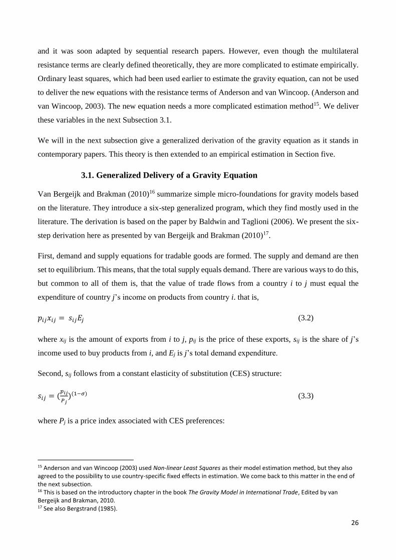
First, demand and supply equations for tradable goods are formed. The supply and demand are then
set to equilibrium. This means, that the total supply equals demand. There are various ways to do this,
but common to all of them is, that the value of trade flows from a country i to j must equal the
expenditure of country j’s income on products from country i. that is,
𝑝𝑖𝑗𝑥𝑖𝑗 = 𝑠𝑖𝑗𝐸𝑗 (3.2)
where xij is the amount of exports from i to j, pij is the price of these exports, sij is the share of j’s
income used to buy products from i, and Ej is j’s total demand expenditure.
Second, sij follows from a constant elasticity of substitution (CES) structure:
𝑠𝑖𝑗 = (𝑝𝑖𝑗
𝑃𝑗)(1−𝜎) (3.3)
where Pj is a price index associated with CES preferences:
15 Anderson and van Wincoop (2003) used Non-linear Least Squares as their model estimation method, but they also agreed to the possibility to use country-specific fixed effects in estimation. We come back to this matter in the end of the next subsection. 16 This is based on the introductory chapter in the book The Gravity Model in International Trade, Edited by van Bergeijk and Brakman, 2010. 17 See also Bergstrand (1985).
27
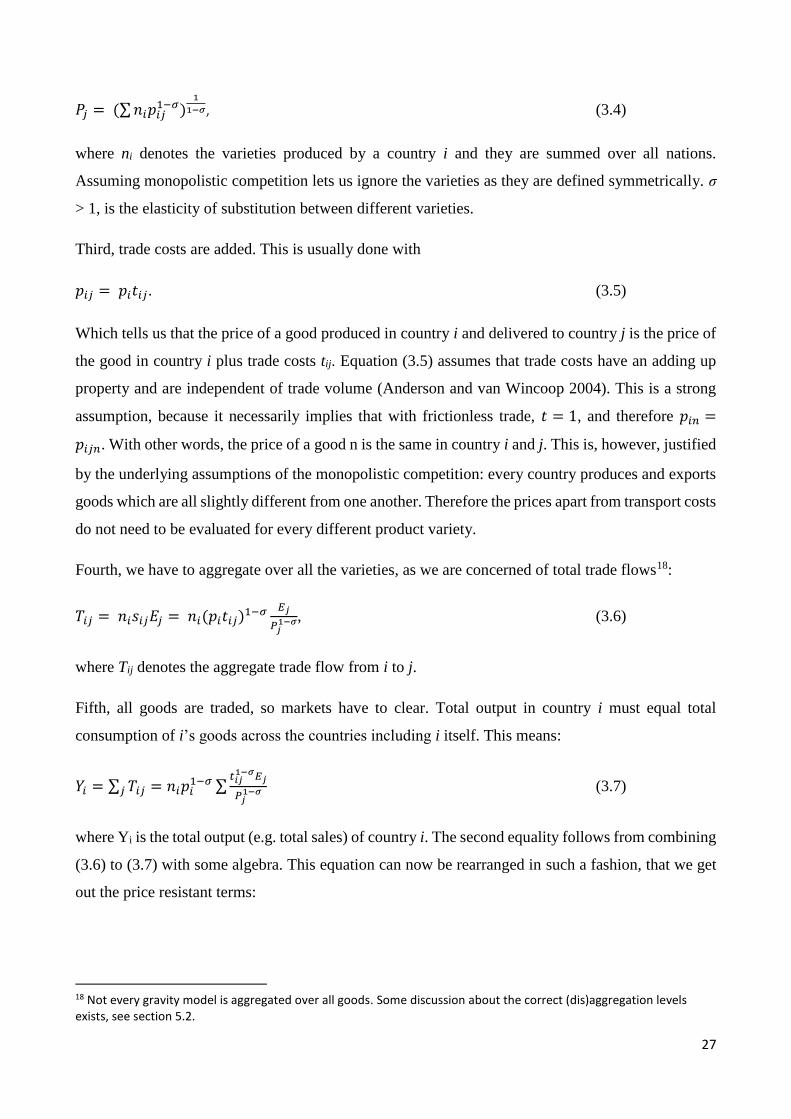
𝑃𝑗 = (∑ 𝑛𝑖𝑝𝑖𝑗1−𝜎)
1
1−𝜎, (3.4)
where ni denotes the varieties produced by a country i and they are summed over all nations.
Assuming monopolistic competition lets us ignore the varieties as they are defined symmetrically. σ
> 1, is the elasticity of substitution between different varieties.
Third, trade costs are added. This is usually done with
𝑝𝑖𝑗 = 𝑝𝑖𝑡𝑖𝑗. (3.5)
Which tells us that the price of a good produced in country i and delivered to country j is the price of
the good in country i plus trade costs tij. Equation (3.5) assumes that trade costs have an adding up
property and are independent of trade volume (Anderson and van Wincoop 2004). This is a strong
assumption, because it necessarily implies that with frictionless trade, 𝑡 = 1, and therefore 𝑝𝑖𝑛 =
𝑝𝑖𝑗𝑛. With other words, the price of a good n is the same in country i and j. This is, however, justified
by the underlying assumptions of the monopolistic competition: every country produces and exports
goods which are all slightly different from one another. Therefore the prices apart from transport costs
do not need to be evaluated for every different product variety.
Fourth, we have to aggregate over all the varieties, as we are concerned of total trade flows18:
𝑇𝑖𝑗 = 𝑛𝑖𝑠𝑖𝑗𝐸𝑗 = 𝑛𝑖(𝑝𝑖𝑡𝑖𝑗)1−𝜎 𝐸𝑗
𝑃𝑗1−𝜎, (3.6)
where Tij denotes the aggregate trade flow from i to j.
Fifth, all goods are traded, so markets have to clear. Total output in country i must equal total
consumption of i’s goods across the countries including i itself. This means:
𝑌𝑖 = ∑ 𝑇𝑖𝑗𝑗 = 𝑛𝑖𝑝𝑖1−𝜎 ∑
𝑡𝑖𝑗1−𝜎𝐸𝑗
𝑃𝑗1−𝜎 (3.7)
where Yi is the total output (e.g. total sales) of country i. The second equality follows from combining
(3.6) to (3.7) with some algebra. This equation can now be rearranged in such a fashion, that we get
out the price resistant terms:
18 Not every gravity model is aggregated over all goods. Some discussion about the correct (dis)aggregation levels exists, see section 5.2.
28
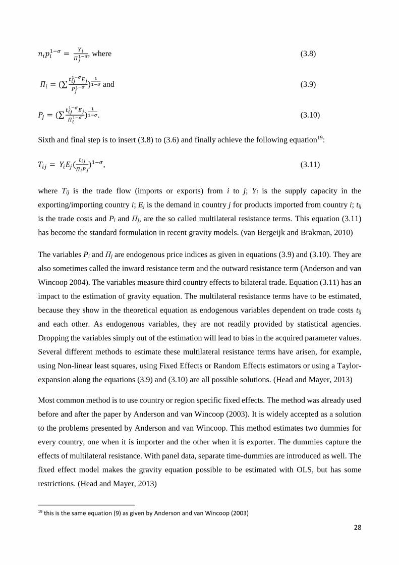
𝑛𝑖𝑝𝑖1−𝜎 =
𝑌𝑖
𝛱𝑗1−𝜎, where (3.8)
𝛱𝑖 = (∑𝑡𝑖𝑗
1−𝜎𝐸𝑗
𝑃𝑗1−𝜎 )
1
1−𝜎 and (3.9)
𝑃𝑗 = (∑𝑡𝑖𝑗
1−𝜎𝐸𝑗
𝛱𝑖1−𝜎 )
1
1−𝜎. (3.10)
Sixth and final step is to insert (3.8) to (3.6) and finally achieve the following equation19:
𝑇𝑖𝑗 = 𝑌𝑖𝐸𝑗(𝑡𝑖𝑗
𝛱𝑖𝑃𝑗)1−𝜎, (3.11)
where Tij is the trade flow (imports or exports) from i to j; Yi is the supply capacity in the
exporting/importing country i; Ej is the demand in country j for products imported from country i; tij
is the trade costs and Pi and Πj, are the so called multilateral resistance terms. This equation (3.11)
has become the standard formulation in recent gravity models. (van Bergeijk and Brakman, 2010)
The variables Pi and Πj are endogenous price indices as given in equations (3.9) and (3.10). They are
also sometimes called the inward resistance term and the outward resistance term (Anderson and van
Wincoop 2004). The variables measure third country effects to bilateral trade. Equation (3.11) has an
impact to the estimation of gravity equation. The multilateral resistance terms have to be estimated,
because they show in the theoretical equation as endogenous variables dependent on trade costs tij
and each other. As endogenous variables, they are not readily provided by statistical agencies.
Dropping the variables simply out of the estimation will lead to bias in the acquired parameter values.
Several different methods to estimate these multilateral resistance terms have arisen, for example,
using Non-linear least squares, using Fixed Effects or Random Effects estimators or using a Taylor-
expansion along the equations (3.9) and (3.10) are all possible solutions. (Head and Mayer, 2013)
Most common method is to use country or region specific fixed effects. The method was already used
before and after the paper by Anderson and van Wincoop (2003). It is widely accepted as a solution
to the problems presented by Anderson and van Wincoop. This method estimates two dummies for
every country, one when it is importer and the other when it is exporter. The dummies capture the
effects of multilateral resistance. With panel data, separate time-dummies are introduced as well. The
fixed effect model makes the gravity equation possible to be estimated with OLS, but has some
restrictions. (Head and Mayer, 2013)
19 this is the same equation (9) as given by Anderson and van Wincoop (2003)
29
Other elegant way to simplify Anderson and van Wincoop is a linearization of trade costs, used for
example by Baier and Bergstrand (2007). A model following Baier and Bergstrand uses a Taylor
expansion to trade costs which simplifies the original Anderson and van Wincoop model and makes
it possible to be estimated with OLS. Baier and Bergstrand show that the model arrives to
approximately same results as the two step way of Anderson and van Wincoop (2003), but is easier
to estimate. (van Bergeijk and Brakman, 2010)
3.2. Gravity Equation with a Single Exporter and/or Importer
For most of the history of this equation, gravity has been used with multi-country data. Multi-country
models have all the countries to export to every other country simultaneously. The estimation results
are then attained on average without making difference between countries. The popularity of this
method is explained by the fact that gravity models have been widely used to estimate policy effects,
such as impacts of free trade agreements or currency unions. In such estimations the impact to a single
partner country is not relevant, when the research question considers the gains from the agreement as
a whole. (Földvári 2006; Sohn 2005)
By estimating the gravity equation with only one exporter (or importer) slightly differs from the
estimation of multi-country models. Multi-country models assume, that every country in the data both
exports and imports. When these flows are accounted simultaneously, they have to equalize. That is,
exports from i to j have to equal imports from i to j. This is often regarded as “symmetry” but in
practice it means that one always estimates either exports or imports and never both. The single
country approach allows to compare country’s imports and exports separately. (Földvári 2006)
An important problem arises with the multilateral resistance. As noted above, the multilateral effects
have been lately estimated mostly with country-specific fixed effects, with year specific fixed effects
in case of panel data. However, this approach is somehow problematic, when estimating the single-
country model. Because the exporter (or importer) stays the same in the whole dataset, using dummy
variables for all the importer (exporter) countries makes it impossible to give reasonable explanations
to time-invariant variables such as distance. The same is true with exclusively time-variant variables
in case of time-dummies, for example, the single exporter economic mass when the exporter is always
a pre-defined single country (Finland in our estimation in Section 6). In panel data analysis one cannot
simply include country-specific dummies with time-invariant variables and time-dummies with time-
invariant variables and then proceed to read the coefficients. Other adjustments have to be made.
(Földvári 2006)
30
Földvari (2006) discusses the implications of single country approach. He estimates static and
dynamic panel models with respect to the Netherlands’ trade. He overcomes the model identification
problems by mixing in a model introduced by Mundlak (1978). He adds the means of the time-variant
variables to the estimation for control20. Estimation is done by random effects estimator instead of
fixed. Variables also include time trends to control for time, because year-dummies would make only
time-variant variable estimates biased. He concludes the model to be correctly specified in
econometrical terms. He also approves the dynamic model over the static model.
Sohn (2006), however, regards the problems with multilateral resistance minor, and proceeds to
introduce a model without specifying country specific effects. His model is cross-sectional and he
discards the multilateral resistance unimportant simply because the relative distances are already
captured in the distance coefficient, which he gives a different interpretation. His model is a static
one-period model and we will not follow his footsteps. However, we point to the fact that regarding
the single country approach and the models generated lately, this kind of denial of multilateralism is
not uncommon.
In the Section 5 we introduce our empirical model. Because of the problem with multilateral
resistance, we follow the example of Fördvári (2006). We generate a random effects panel data model
where Finland is sequentially the sole exporter and importer. The results are then presented in the
Section 6 and discussed in Section 7. The next Section 4 gives a short overhaul of the Finnish
economy and trading sector.
20 This is not to be confused with demeaning. Demeaning subtracts the arithmetic mean of all the variables before estimation. However, this also cancels the time-invariant variables out of the estimation and effectively produces a fixed effect estimator. (Hill, Griffiths and Lim 2008) See Appendix A.2.
31
4. Finland in the World Trade
In this section, we give a picture of the economy of Finland in a nutshell. We try to characterize
Finnish economy and its exports and imports sectors.
Finland is a developed economy in Northern Europe. It joined the European Union in 1995 and
adapted Euro as its currency together with 11 other Union states in 1999 (with euro as a physical
currency from 2002 onwards). In 2011 it had a population of 5.4 million and nominal GDP of $209
billion (in 2005 US dollars) and a GDP per capita $45 741 (in 2005 US dollars). (Statistics Finland,
National Accounts)
Industry (TOL 2008) 2011
Agriculture, forestry and fishing (A) 2.9
Mining and quarrying (B) 0.4
Manufacturing (C) 16.6
Electricity, gas, steam and air conditioning supply (D) 2.3
Water supply; sewerage, waste management and remediation activities (E) 0.9
Construction (F) 6.8
Wholesale and retail trade; repair of motor vehicles and motorcycles (G) 10.3
Transportation and storage (H) 5.4
Accommodation and food service activities (I) 1.7
Information and communication (J) 5.1
Financial and insurance activities (K) 2.9
Real estate activities (L) 12.2
Professional, scientific and technical activities (M) 4.6
Administrative and support service activities (N) 3.5
Public administration and defence; compulsory social security (O) 6.2
Education (P) 5.2
Human health and social work activities (Q) 9.9
Arts, entertainment and recreation (R) 1.3
Other service activities (S, T) 1.9
Gross domestic product at basic prices 100
Primary production 2.9
Secondary production 27.1
Services 70.0
Table (4.1) Finnish value added sorted by industries as a percentage of total value added in 2011.
Source: Statistics Finland, National Accounts.
Table (4.1) shows the composition of Finnish economy in 2011. 70 % of the GDP comes from service
sector, while the share of primary production in GDP is only 2.1% of total. The rest of the value added
comes from the secondary production. The share of secondary production of total value added
(27.1%) is relatively high among industrialized countries. The size of the manufacturing sector is
partly explained by the tradable commodities. Table (4.2) shows the composition of Finnish supply
and demand and the relative shares of exports and imports in 2011, respectively.
32
2011
€ billion %
Supply
GDP 188.7 70.6
Imports 78.7 29.4
Total supply 267.4 100
Demand
Exports 77.3 28.9
Consumption expenditure 151.3 56.6
– private 105.1 39.3
– government 46.2 17.3
Gross fixed capital formation 36.7 13.7
– private 31.9 11.9
– government 4.7 1.8
Changes in inventories, acquisition of valuables 2.1 0.8
Total demand 267.4 100
Statistical discrepancy 0.0
Table (4.2) Finnish national balance of supply and demand in 2011. Source: Statistics Finland,
National Accounts.
Both the imports and exports amount to a nearly 30% share of the total supply and demand. A rough
third of the Finnish production is pointed towards demand from abroad. These figures show how
Finland is a small economy, which is highly dependent of the exports sector. The current account had
turned to deficit in year 2011 after years of surplus. We turn next to the composition of Finnish exports
and imports as they are in the focus of this paper. (Statistics Finland, National Accounts)
Table (4.3) shows the main groups of Finnish exports. The main exporting sector is the industry of
chemical products, shortly followed by forest industry. Forest industry has been the primary export
industry for centuries due to the scarcely populated land and its large forest coverage. In 1950 the
forest industry accounted for 85% of Finnish trade, while in 201321 the share had declined to 20%.
(Statistics Finland, National Accounts) Since 1950’s, the focus has shifted inside the industry from
timber and primitive paper to more advanced paper products such as packing material and coated
paper incorporating a higher value added. Adding to the success of forestry are the forest friendly
soil structure, easy access to even to the most remote forests due to the natural waterways and the
scattered ownership of private forests keeping farmers interested in the forest business. (Solsten and
Meditz, 1990)
Exports € million %
Chemical industry products 13.806 24,7
Forest industry products 11.221 20,0
21 estimate
33
Metal and metal products 7.958 14,2
Machinery and equipment 7.513 13,4
Electric and electronics industry products 6.395 11,4
Other 9.100 16,3
Imports € million %
Chemical industry products 12.439 21,4
Products from mining and quarrying 10.217 17,5
Electric and electronics industry products 6.926 11,9
Transport equipment 4.753 8,2
Machinery and equipment 4.652 8,0
Other 19.250 33,1
Table (4.3) Finnish exports and imports sorted by industry. An estimate for the year 2013. Source:
Statistics Finland, National Accounts.
However the historical importance of forestry, chemical manufacturing has driven past the
importance of forest industry as the main export factor. The picture (4.1) shows the composition of
the exports of the industry. Oil products and basic chemicals account for nearly 60% of the total.
Pharmaceutical products follow as the third biggest group with a share of 16% of total.
Picture (4.1). The composition of Finnish chemical industry exports in 2012. Source: The Chemical
Industry Federation of Finland (Kemianteollisuus).
Metal, machinery and electronics industries come shortly behind the first two, together accounting
for over one third of the total imports. The metal industry evolved fast after the Second World War
as a result of heavy preparations paid to Soviet Union. In the metal industry the shift has also been
34
from basic metal products to more sophisticated machinery and electronics, incorporating a higher
value added. (Solsten and Meditz, 1990) Product examples include electrical transformers, passenger
and cargo ships and telephones. (Observatory of Economic Complexity)
The chemical industry products are also the most important sector of imports. This hints towards the
models of monopolistic competition, which predict Finland to import similar products as it produces
and exports. The same can be said about the class “Electronic and electronics industry products”. The
same class is presented in both imports and exports with an eleven percent share. Products of mining
and quarrying is the second biggest group, which in turn hints to the H-O model. Countries with
abundant resources tend to export these resources and countries scarce of the same resources tend to
import them. Trade in forest industry products also echoes the predictions of H-O. While heavily on
the export side, the industry is not important in the import side.
With which countries does Finland trade? The classical gravity equation predicts that a country should
trade more with large economies which are close to its borders, than with small economies which are
far away. Picture (4.2) maps the world economies and their imports from Finland in 2012.
Picture (4.2) Map of importing markets for a product exported by Finland in 2012. Source: UN
COMTRADE statistics. The picture provided by Trade Map.
35
The map shows that in 2012 Finland indeed exported more to countries with shared border (Sweden,
Norway, Russia and Estonia) than to similar countries further away. It also shows that Finland
exported more to relatively large economies (such as United States, Brazil, Japan or China) than to
relatively smaller economies as far away as the larger ones. Overall it seems like the most important
import markets can be found in West Europe along with the rich industrialized countries around the
globe.
Picture (4.3) shows the exporters for a product imported by Finland during the same period. Similar
conclusions may be drawn as with the exports. Proximity seems to increase trade along with the size
of the exporter. We like to make some extra remarks. First, distance seems to kill the imports faster
than the exports. Second, some outliers remain, for example, Republic of Congo seems to export to
Finland more than its relatively similar neighbors, even though it is a relatively distant and small
economy. We believe this hints to the specialization discussed among Heckscher-Ohlin model in
Section 2. With other words, Republic of Congo is highly abundant of resources imported by Finland
in a way that simple economic geography cannot explain. Again, most of the trade seems to be with
developed industrialized countries.
Picture (4.3) Map of exporting markets for a product imported by Finland in 2012. Source: UN
COMTRADE statistics. The picture provided by Trade Map.
36
To summarize, Finland is a small economy heavily dependent on trade. Finland exports goods based
on its abundant forests and imports raw materials based on the scarcity of domestic production,
according to predictions by H-O model. On the other hand, Finland trades heavily in advanced
chemical, metal, mechanical and electronic products both importing and exporting them, according
to monopolistic competition models. The most important trading partners are her neighbor
economies, EU and rich OECD economies around the world.
In the next section we proceed to derive an empirical estimation of Finnish trade and present the
attained results in Section 6.
37
5. The Empirical Model
In this empirical section, we first lay down our questions and hypothesis. Then we build our model
by introducing the variables and coefficients to be estimated. We convert the model introduced in the
previous section to an empirical model which is then used to deliver results. We present the results in
the Section 6.
The hypothesis which we are to test is:
Hypothesis: The elasticity of exports and the elasticity of imports subject to the distance is the same
for Finland as it is found to be in literature in general.
We build two gravity models. The first model incorporates Finland as the sole exporter. In this dataset,
only Finnish exports are to be accounted and the exports from importer countries are not accounted
for. The second model incorporates Finland as the sole importer. The used dataset stays otherwise the
same, only imports are now used instead of exports. This is a single-country model. To compare the
results in literature we review the meta-analysis by Head and Meyer (2013) to find corresponding
estimates to our two models. Additionally, we revise the results attained by Földvári (2006), because
of methodological similarity. Against this background, we can reassess the hypothesis and convert it
to the following questions:
1. Does the estimated distance coefficient for Finland as a sole exporter in the dataset correspond
the value of the distance coefficient when Finland is the sole importer?
2. Does the above mentioned distance coefficient for Finland as the sole exporter and as the sole
importer correspond to the values found in literature by Head and Meyer (2013) and Földvári
(2006)?
We expect to find that Finnish distance coefficient is negative and closely related to estimates found
in earlier papers. The export-import difference is solely to be found out and we lay no forecasts to it,
simply because there has not been earlier papers to compare with.
In the following subsections we generate the models by first introducing the variables, followed by
description of the datasets. We then shortly discuss about the short-comings of the models and answer
possible criticism.
38
5.1. Variables
We take the natural logarithm of the equation (3.11), add the time dimension with subscript t and
drop the subscripts i and j of P and Π for the ease of notation, we have the following presentation:
Distancej follows the example of Head and Mayer (2002). The calculated bilateral distance of two
countries is based on the bilateral distance of the largest cities of the respective countries. The intra-
country bilateral distances between cities are weighted by the country’s population distribution. Head
and Mayer provide the formula:
𝐷𝑖𝑠𝑡𝑎𝑛𝑐𝑒𝑗 = ((∑𝑃𝑂𝑃𝑘
𝑃𝑂𝑃𝑖∑
𝑃𝑂𝑃𝑙
𝑃𝑂𝑃𝑗)𝐷𝑖𝑠𝑡𝑘𝑙
𝜃 )1
𝜃 (5.4)
where k is a city in country i, POPk denotes population23 in a city k, l is a city in country j and POPl
denotes the population in city l, Distkl is the great circle distance between the cities in both countries
in kilometers. As we see, the population weighted bilateral distances are summed over all cities in i
and j. The parameter θ denotes the sensitivity of trade to bilateral distance and usually takes the value
of either 1 or -1. We have a sensitivity coefficient set as -1, as provided by our data source. Measuring
the distance as an average of economic centers provides more robust estimation especially in case of
countries, which have several important centers of trade. (Head and Mayer, 2002)
Distancej acts as an approximation for increasing trade cost. The longer the distance, the costlier is
the transportation in real terms such as transportation costs, fuel or time. Cultural distances probably
also affect the relative trade costs and these costs may not be linear. We take a rather unrealistic
approach, where cultural distances are assumed linear with geographical distance. Some distinctive
22 Great circle distance is the distance measured along the atmosphere of Earth. This is not a straight, but a circular line, as the Earth is not flat. The measurement line may cross the Polar Regions, as it is measured where the distance is the shortest. 23 Head and Mayer (2002) had country GDP’s in their equation instead of population, but our data contains the distances weighted by population.
40
ways to overcome this problem have been proposed, but they are beyond the reach of this paper24.
(Novy, 2012)
Border dummy takes the value of 1 if countries are adjacent to each other or separated by a small
body of water and 0 otherwise. Border dummy is added for two reasons. First, countries trade more
with their neighbor countries. This is of course linked to the distance parameter, but border dummy
tends to stay statistically significant even when estimated with a distance parameter. This hints to
think that trade may benefit from the adjacency by more than with just the close distance. The strong
positive and statistically significant estimates in the literature motivates us to include this term. We
expect the sign of the coefficient to be positive. (Head and Mayer, 2002 and 2012)
EU dummy takes the value of 1 if the partner country belongs to EU and 0 otherwise. Free trade
agreements (FTA) tend to be positively correlated with increased trade, which makes sense as the
reason to belong to a FTA is to ease trade between countries. Belonging to a FTA rises some questions
of endogeneity, as countries who share strong trade links are more likely to enter a FTA than countries
which do not. Some of the countries in the dataset joined EU over the time interval, but because of
the possible uncontrolled endogeneity, the estimated coefficients should be read cautiously.
Nevertheless, we expect the sign of this coefficient to be positive. (Baier and Berstrand, 2004)
EFTA dummy takes value 1, when the partner country belongs to European Free Trade Agreement
and 0 otherwise. This means Norway and Switzerland in our data. We include the EFTA variable as
the EFTA members have similar barriers to trade with EU countries as EU member states themselves
have. Therefore, we expect it to have similar effects to trade as the EU variable. No changes in the
status exists in the covered time period.
EURO dummy takes the value 1 if country has euro as its currency and 0 otherwise. Shared currency
is anticipated to ease and hence increase trade between two countries. As with the EU membership,
some countries took up the Euro as their national currency over the course of the covered time period.
The same problem with possible endogeneity applies here, and we proceed with caution when
interpreting the results. We expect to have a positive sign.
To complement our estimation in section 6 we include a price index variable in an auxiliary equation.
This variable uses the United States of America (=100) as a base country to evaluate the relative
prices of the trading countries in the dataset. This Price variable is a measurement of relative prices
24 See for example Möhlman et al (2009), or Rauch (1999).
41
and uses the Geary-Khamis method to compute the values. The base country USA always has an
index value of 100 thorough the dataset.
The reason to leave this variable outside of our main estimation is twofold: first, our data is limited
and including the price index means dropping the two last years from the dataset. Second and more
importantly, the variable is not theoretically needed. As we show below, the inclusion of country
specific means and using random effects estimator is enough to bear the influence of country specific
(price) effects. There exists discussion about the available price indices used with gravity equations
and generally they are disliked in the literature. (Baier and Bergstrand 2001) This is due to the
composition of the price indices, which seldom takes in the account the composition of trade and is
biased towards non-tradable goods. The consumer price indices are problematic in the concept of
trade costs, as they take in the account the different levels of local costs, taxes and subsidies.
(Anderson and van Wincoop 2004)
We include this variable as a reference and for the possible added explanatory force. With Price, our
where Pricej is the price index in country j and ρ is the coefficient to be estimated.
Together the trade cost function is an approximate of the trade costs between two countries. It presents
a point estimate of the ceteris paribus trade barriers between countries. Similar trade cost functions
have been used to summarize the trade costs in previous papers. For example, the meta-analysis of
Anderson and van Wincoop (2004) presents an average point estimate of 170% for trade barriers
collected from literature. As an example of this we present our own point estimate of trade costs
between Finland and Sweden in the chapter 6.
Distancej is a continuous variable and hence in logarithmic form as the general equation (5.1). This
allows us to plug the equation (5.3) into the equation (5.2) without problems. We can then regard the
coefficient of distance as elasticity. It is the elasticity of trade with respect to distance.25
ln tij(1-σ) is now substituted into the equation (5.2) as:
25 We leave the discussion of the functional form in gravity equations outside of the paper. See for example Bosker and Garretsen (2009), Anderson and van Wincoop (2004) or Hummels (2001)
leads to possibly a very large bias in estimation of distance coefficient as short distances are
overrepresented. Other possible way is to add an arbitrarily small amount of trade in place of the non-
existent trade. (van Bergeijk and Brakman 2010) Our dataset does not contain zero flows. However,
limiting the dataset to not contain zero flows might be seen generating the same problems as a census
approach with zero flows dropped out. We bear this in mind when discussing the results in Section
7.
The problem of measuring distance is part of a series of problems linked with estimating the trade
costs. Specification of the trade cost function differ from paper to paper and therefore the importance
of distance also varies accordingly. As distance plays a role in estimating the trade costs, the
measurement of distance affects the trade function. What preludes this problem is the fact that real
trade cost data is extremely hard to find. We have chosen the measurement introduced by Head and
Mayer (2003), because it gives intuitively better presentation of the links between countries economic
centers than the straight-forward and primitive measurement of bilateral distance between capitals.
However, different measurements of distance exist in the literature and our way is chosen partly
arbitrary. (Head and Mayer 2010)
The correct level of aggregation in estimation is of course subject to the questions posed to the
research in hand. However, trade data is known to be subject to large accounting bias (Hummels 1999
Appendix II). Mostly used aggregation levels are country level and industry level. More disaggregate
data is often considered too biased. On the other hand, country level data is subject to the problem of
specifying the correct elasticity of substitution σ, as it fluctuates between industries. (Anderson and
van Wincoop 2004). We have chosen the country level (and annual) data simply because the research
question is not industry-specific. More disaggregate level would also be possible.
The parameter σ is the elasticity of substitution between tradable goods. The size of this coefficient
matters as it enters the theoretical equation (3.11) and equation (5.3). However, it does not impact the
estimation. When σ is sufficiently high or indefinite, it makes the trade cost function obsolete (tij
approaches zero). In general, the higher the elasticity coefficient is, the smaller the trade barriers get
(tij gets smaller). There exist several ways to estimate the coefficient σ and a subsequent discussion
about it, but as Anderson and van Wincoop (2004) note in their literature review in the chapter
covering the topic, most estimation results range between 5 and 10. Because the estimation of this
coefficient is beyond the range of this paper, we let σ to take a value of 8 when interpreting the total
48
effects of trade costs in the Section 7. This is an approximation which is close to the results presented
by several authors.26
There are several variables, which are common in the literature, but which we have dropped from the
estimation as unimportant. One of these is common language dummy which is dropped for the simple
reason that Finnish is not widely spoken outside of Finland. Swedish as the second official language
in Finland might be used, but we believe its inclusion would be trivial and pose problems when
defining the variable.
A second example is a variable for colonial ties. This is dropped practically for the same reason as
the language dummy. Although a shared history with Sweden or Russia might be accounted for, we
regard such old links as trivial27. More importantly, this kind of dummy is normally used between old
colonial masters and their colonies which have gained independence rather lately, such as the old
British Empire with its countless colonies all around the world. We do not see a need for this extra
variable.
Real (Effective) Exchange Rate is often included in the trade cost function to account for price
changes in the data. However, we have left the variable outside of our estimation generally for the
same reasons as the Price variable. Including this variable is dubious, taken that we have accounted
for the country-specific effects. The inclusion of the Price variable in the auxiliary model serves as
an add-on to take into account the relative price changes. Therefore we see no reason to include one
more variable.
GDP and GDP per capita are somewhat endogenous with respect to imports and exports through the
identity equation: 𝑌 = 𝐶 + 𝐼 + 𝐺 + (𝑋 − 𝑀). There exist several papers which have addressed the
problem by introducing instrumental variables with respect to GDP28. However, the results show that
the endogeneity bias appears to be small and negligible. Therefore we have not addressed the problem
in this paper and assume the GDP and GDP per capita to be sufficiently exogenous. (Cyrus 2002;
Hummels and Levinsohn 1995, Frankel 1997)
26 For example: Hummels (2001a): 8.26, with one digit SITC data; Head and Ries (2001): 7.9 with fixed effects; Eaton and Kortum (2002): 9.28. (Anderson and van Wincoop, 2004) 27 Because of the shared history with both Sweden and Russia, which take up two thirds of the countries neighboring Finland, this effect is partly captured in the border dummy. 28 See for example a paper by Cyrus (2002). She notes that although using factor endowments in place of GDP provides better estimates, the bias compared to OLS seems to be small.
49
6. Results
We estimated the model specified in equation (5.10) two times. Additively, we estimated some
auxiliary models to compliment the main Export- and Import-model. In the Export-model the
regressant ln Tijt represents the export flows from Finland (Exportjt) and in the Import-model the
import flows (Importjt). Otherwise the variables presented in equation (5.10) stay the same. In this
section we go through the estimation results. We start by searching for a reference point in literature.
Next we estimate the Export-model with all the included variables. This is then repeated with the
Import-model.
6.1. Literature
Head and Meyer (2013) revisited estimation results of the most common variables in gravity
equations. Based on 2508 estimates from 159 papers, they present the following table:
Table (6.1). Meta-analysis by Head and Meyer (2013).
Table (6.1) shows the aggregated results of most common variables attained from 159 papers. In the
first four columns they list averaged values attained from data without making a difference between
methods. The columns 5-8 show averaged results attained from models using “structural gravity”.
This structural gravity refers to two methods: using country-specified fixed effects or ratio-type
method. Fixed effect estimator is explained in Appendix (A.2). Ratio-type method is similar to fixed
50
effect, but tries to reduce the computational need by normalizing the equation to be estimated. This
is done by using the attributes of one market as a common numeraire, therefore reducing the elements
to be estimated.29 Our estimation is not structural in this sense. It does not involve fixed effect nor
ratio-type estimation, albeit random effects estimator has a close linkage with FE. Therefore we see
the variable averages gathered from all types combined in columns 1-4 in table (6.1) a better reference
point as the limited set in columns 5-8. It should also be noted, that all these estimates in Table (6.1)
are mainly from multi-country models.
The estimates which interest us the most in this table, are the coefficient estimates for the Distance
variable. The coefficient mean is -0.93 (std.err. = 0.40) when all different kind of gravity equations
are accounted for. Median effect is slightly less strong, -0.89.
This works as a reference point to the estimates acquired from our models. However, because the
meta-analysis by Head and Mayer (2013) is not limited to single-country-models, we also show the
results attained by Fölvári (2006) subject to trade of the Netherlands. This is also a good alternative
reference point, because we used the exactly same methodology in our estimation.
Fördvári (2006) estimates a static model separately for exports and imports like us30. The estimated
coefficient for distance is -0.546 (std.err. = 0.113) for exports and -0.253 (std.err. = 0.148) for imports.
These are much smaller effects than found by Head and Mayer (2013). Especially the effect of
distance on imports is more than one and a half standard deviation less than the average found by
Head and Mayer. Bearing these results in mind, we proceed to estimate our models.
6.2. Finland as the Sole Exporter
6.2.1 Main Export-model
ln 𝐸𝑥𝑝𝑜𝑟𝑡𝑠𝑗𝑡 = 𝛼0𝑋 + 𝛼1
𝑋 ln 𝐺𝐷𝑃𝑗𝑡 + 𝛼2𝑋 ln 𝐺𝐷𝑃𝑃𝑗𝑡 + 𝛼3
𝑋 ln 𝐷𝑖𝑠𝑡𝑎𝑛𝑐𝑒𝑗 + 𝛼4𝑋 𝑏𝑜𝑟𝑑𝑒𝑟𝑗 +
𝛼5𝑋𝑒𝑢𝑗𝑡 + 𝛼6
𝑋𝑒𝑓𝑡𝑎𝑗 + 𝛼7𝑋𝑒𝑢𝑟𝑜𝑗𝑡 + 𝛼8
𝑋 𝐺𝐷𝑃̅̅ ̅̅ ̅̅𝑗 + 𝛼9
𝑋𝐺𝐷𝑃𝑃̅̅ ̅̅ ̅̅ ̅̅𝑗 + ∑ 𝛼9+𝑡
𝑋𝑇𝑡=1 𝑦𝑒𝑎𝑟𝑡 + 𝜀𝑗𝑡
𝑋, 𝑡 =
1, … , 𝑇 = 2001, … , 2012 𝑗 = 1, … , 39. (6.1)
Our first estimated model is the equation (5.10) using Finnish annual exports in the time interval
2001-2012 as the regressant ln Tijt forming equation (6.1). Graph (A.1.1.) in Appendix shows
29 There is exists a multitude of ratio-type methods. For a better look on the topic, see Head and Mayer (2013). Most importantly the ratio-type method is similar to fixed effects estimation, which is explained in Appendix (A.2) 30 Fördvári (2006) also introduced a dynamic model including a certain amount of lags of the regressant. In this dynamic approach the distance coefficient took a value of -0.011 for exports and 0.014 for imports. These estimates are not statistically significant.
51
Distance on the x-axis plotted against Exports on the y-axis, Graph (A.1.2.) importer GDP plotted on
the x-axis against Exports on the y-axis and Graph (A.1.3.) plots the importer GDP per capita against
Exports in a similar manner. All four variables are in logarithmic form. The graphs show how there
seems to be a slight negative relation between Distance and Exports, and slight positive relation
between importer GDP and Exports, respectively. We proceed to estimate the equation (6.1). The
coefficient estimates are shown in Table (6.2).
Variable Coefficient Estimate
Standard Error(1)
t-statistic p-value
Intercept 10.0187 1.1491 8.7187 0.0000 ***
Distance -0.7581 0.0930 -8.1498 0.0000 ***
Importer GDP 0.2698 0.1818 1.4841 0.1385
Importer GDP per capita
0.6445 0.6445 0.0956 0.0000 ***
Border 0.7777 0.2164 3.5936 0.0003 ***
EU -0.1903 0.0525 -3.6284 0.0003 ***
EFTA -0.8851 0.2677 -3.3059 0.0010 **
EURO 0.0596 0.0985 0.6250 0.5455
/ / / /
F-statistic (on 20 and 447 DF)
50.9509***
TSS 68.97
RSS 21.029
R-Squared 0.69509
Adj. R-Squared 0.6639
Table (6.2). The estimation results of Equation (6.1) using Finnish exports as Tijt on all the
variables introduced in Section 5. (1) White’s heteroskedasticity-consistent standard errors.
Table (6.3) Breusch-Pagan test for residual heteroskedasticity. HA: Heteroskedastic residuals.
Source: data.
52
Table (6.3) shows the Breusch-Pagan test31 for residual heteroskedasticity. Because the residuals are
heteroskedastic, we use the White’s heteroskedasticity-consistent standard errors32 in table (6.2).
Except Importer GDP and EURO, all the variables are statistically significant. EU-dummy and EFTA-
dummy attain an unexpected negative sign, while Distance (-), Importer GDP per capita (+) and
Border-dummy (+) all have expected signs.
Recalling our hypothesis, the most important variable is the Distance. The Distance coefficient is
significant on 0.001% level and attains a value of -0.7581. It is negative as expected and the estimate
is 43.8 % of a standard error from the median of the estimates provided by Head and Mayer.
Border dummy is statistically significant and has a coefficient value of 0.7777. It is positive as
expected. Adjacency has a slightly stronger impact in our estimation than on average in the meta-
analysis of Head and Mayer (contiguity). Nevertheless, the impact of adjacency is as expected.
EU and EFTA dummies are both statistically significant, while EURO is not. However, the impact of
both EU and EFTA is negative. The negative impact of EFTA seems to be implausible strong. This is
unexpected as we waited for a positive signs. EU has a coefficient of -0.1903, while EFTA coefficient
is -0.8851. This would mean that belonging to European Union or to European Free Trade Area
decreases trade compared to similar economies as far away. This is a disturbing result, but as we
warned in Section 5, one should not take neither of these estimates too seriously, as they may be
subject to severe endogeneity bias, which has been left uncontrolled for in this estimation.
The Average Importer GDP (not shown) is not statistically significant, while the Average Importer
GDP per capita (not shown) is. This is in line with Importer GDP and Importer GDP per capita
estimates. The former is significant, while the latter is not. The two variables were called for control
of country specific effects and we may draw a conclusion that such country specific effects exists in
the data. The R-Squared of the estimation is 0.69509 (Adj. R2=0.6639).
We also estimated 11 time dummies taking a value 1 or 0 according to the respective years. This was
done to control the panel data aspects of the model. Year dummies for the years 2004-2008 are
statistically significant having a range from 0.1477 to 0.3134. We believe this reflects the heating of
the economy and increase in trade in the years before the late financial crisis.
31 Breusch-Pagan test for heteroskedasticity uses the variables in the estimated equation to estimate the residuals of the same equation. The test statistic is given by N*R2 ~ χ2
(S-1), where N is the sample size, R2 is the goodness-of-fit statistic of this regression and S the number of parameters. (Hill, Griffiths and Lim 2008) 32 White’s heteroskedasticity-consistent standard errors are attained by replacing the variance with the squared residuals of the estimation, when calculating the standard errors. (Hill, Griffiths and Lim 2008)
53
Table (6.4) shows the results of Shapiro-Wilk normality test33 of the residuals attained. We have
chosen the Shapiro-Wilk test because it has been shown to be the most powerful of normality tests34
(Razali and Wah, 2011). The residuals are shown in Plot (6.1) in four different plots. The Shapiro-
Wilk test suggests that the residuals are non-normal on 5 percent level. However, taken the relatively
high test statistic W (>.99), the relatively large dataset (N x T=468) and looking at the Plot (6.1)
allows us to conclude, that the residual distribution is no cause of concern.
Shapiro-Wilk normality test
Residuals attained from Equation (6.1)
Test statistic W p-value H0
0.9919 0.01199 Normally distributed
Table (6.4) Shapiro-Wilk normality test on residuals attained from Equation (6.1). With Price. HA:
Non-normally distributed residuals. Source: data.
33 Shapiro-Wilk normality test compares the cumulative distribution of the test variable with the cumulative distribution of a normal sample. 0 ≤ W ≤ 1, where 1 is a normally distributed sample. For the derivation of the test statistic W, see Shapiro and Wilk (1965). We used the modified test introduced by Royston (1992), which allows the Shapiro-Wilk test for larger samples. 34 We also run Jarque-Bera and Kolmogorov-Smirnov tests of normality for the residuals in every estimated equation in this paper, but did not find any contradicting evidence against the use of Shapiro-Wilk test.
54
Plot (6.1) Export-model residuals. (6.1.1) shows a histogram of residual distribution. (6.1.2) shows
the residuals plotted against their deviation from zero. (6.1.3) shows residual quantiles plotted
against quantiles acquired from standard normal distribution. (6.1.4) shows residuals fitted against
Exports. Source: data.
6.2.2. Auxiliary Export-model with variable Price
As noted earlier in Subsection 5.1 we run an auxiliary model spanning
from 2001 to 2010 with the added variable Price. The variable Price is
described in Table (6.5). The variable is on level instead on logarithm. This
allows the interpretation of the coefficient of Price, multiplied by 100, as
a percentage change in Exports, when the Price index changes by one. We
expect a negative sign, as higher index value means relatively higher
prices. The estimated model is given by equation (6.2). To compare the result, we also run a model
without the Price variable, but also spanning from 2001 to 2010 (N x T = 390). This model presented
in Equation (6.3), therefore looks exactly the same as equation (6.1) only with shorter span for t.
The value of lambda is in central position, when we determine between FE and RE. However, we do
not know the true values of 𝜎𝛼or 𝜎𝑒 and they therefore have to be first estimated36. (Hill, Griffith and
Lim 2008). The estimated variances are then used to substitute the population variables in equation
(A.2.6) and then proceed to estimate �̂�:
�̂� = 1 − (�̂�𝑒
2
�̂�𝑒2+𝑇�̂�𝛼
2)1/2. (A.2.8)
The estimated value of λ allows us now to make a distinction between separate cases. Note that 0 ≤
𝜆 ≤ 1.
We see from the Equation (A.2.8) the main situations when lambda takes a value of 0, 1 or something
in between, and what it means to us. If we remove the term 𝑇�̂�𝛼2 from the formula, the big term in the
right hand side takes a value of 1 and gives us: �̂� = 0. This happens if the variance of 𝛼𝑖 is zero.
Unsurprisingly, if both the expected value and the variance of αi is zero, we can drop the term
altogether. This means that we generate the Equation (A.2.4), only without 𝛼𝑖 as there exists no
individual effects. We can now consistently estimate this with Ordinary Least Squares. There is no
36 A normal procedure is to first estimate a Pooled OLS or a FE model to recover the sample variance estimates,�̂�𝛼 and �̂�𝑒, see the equations for Fixed Effects below.
80
need for FE or RE estimation, if λ, and consequently 𝛼𝑖, turns out to be zero, because The OLS
generates efficient and unbiased estimates of the population values.
When λ is 1 we have Equation (A.2.9). We effectively demean the variables. This implies that all
time-invariable variables get cancelled out of the estimation along with the intercept and 𝛼:
Table (A.2.1) Lagrangian Multiplier test for models presented in Section 6 in main text. LM-test
statistic follows χ2-distribution. Source: data.
Table (A.2.1) shows, that despite the relative large lambdas, random effects are present in the data.
Sources:
R. Carter Hill, William E. Griffiths and Guay C. Lim, 2008, Principles of Econometrics, 3rd Edition.
ISBN: 978-0471-72360-8, Hardback. John Wiley & Sons, Inc, Thompson Digital.
82
thonkane
Text Box
Abstract ITÄ-SUOMEN YLIOPISTO Tiedekunta Yhteiskuntatieteiden ja kauppatieteiden tiedekunta Yksikkö Kauppatieteiden laitos Tekijä Veikko Rautala Työn nimi Ulkomaankaupan gravitaatioyhtälö Etäisyyden vaikutuksen estimointi Suomen ulkomaankaupassa Pääaine Kansantaloustiede Työn laji Pro Gradu -tutkielma Aika 19.02.2014 Sivuja 84 Tiivistelmä Tässä Pro Gradu -tutkielmassa mallinnetaan Suomen ulkomaankauppaa käyttämällä ns. gravitaatiomallia. Tutkielman pääasiallisena tarkoituksena on määritellä etäisyyden vaikutus Suomen ulkomaankauppaan. Työn teoreettisessa osassa esitellään kolmea ulkomaankaupan mallia (Ricardolainen, Heckscher-Ohlin ja monopolistisen kilpailun malli). Mikroteoreettinen pohja empiiriselle estimoinnille rakennetaan seuraten Bergeijk ja von Brakmanin (2010) esittämää yleistystä. Metodina käytetään random effects -estimaattoria ja data käsittää aikavälin 2001-2012 vuositasolla ja sisältää 39 Suomen tärkeintä kauppakumppania. Tulokseksi saadaan, että Suomen vientielastisuus suhteessa etäisyyteen myötäilee Head ja Mayerin (2013) meta-analyysissa saatuja tuloksia. Avainsanat: gravitaatio - Suomen ulkomaankauppa - random effects - etäisyys - maakohtainen