Growing into Export Markets: The Impact Exporting on Firm ...pirical evidence that many new...

Growing into Export Markets:

The Impact Exporting on Firm-Level Investment in Indonesia

Young-Woo Rho† Joel Rodrigue‡

Department of Economics, Vanderbilt University, Nashville, TN, United States

July 6, 2012

Abstract

This paper documents the impact of exporting on capital accumulation across heterogeneousmanufacturing firms in Indonesia. We emphasize that entering export markets significantlychanges investment behavior before, during and after entry into export markets. Accountingfor endogeneity and selection, we provide estimates of the magnitude and duration of therise in investment during entry into export markets. In contrast to many models of firm-leveltrade we find that firms actively expand capacity and increase their holdings of capital stockas they enter export markets. We document that the investment rate among new exportersis 30 percent higher than non-exporters in the year preceding entry, 41 percent higher in theinitial year of entry and 24-27 percent higher in the two years after entry.

Further, we document that foreign and domestically owned firms enter export marketsvery differently. Domestic firms grow capital holdings slowly over time, while foreign firmstend to invest heavily in one or, at most, two years. We find that the impact of exportingon investment among foreign firms is nearly double that of similar domestic firms in theyear of entry into export markets. In all other years around entry into export marketsthere is little statistical evidence of any difference across foreign and domestic firms. Weconfirm that differences across foreign and domestic firms are strongest during periods oftight domestic credit in Indonesia and indicative of impact of credit market imperfectionson export behavior.

Keywords: Investment, Exports, IndonesiaJEL Classification Numbers: D24, F14, F23, O12, O16

Contact Information.

Mailing Address: Department of Economics, Vanderbilt University, VU Station B #351819, 2301 Van-

derbilt Place, Nashville, TN 37235-1819; Tel.: +1 615 322 2871; fax: +1 615 343 8495.

E-mail addresses: †[email protected]; ‡[email protected].

Since the 1960s numerous East Asian countries have witnessed unprecedented economic

growth rates. Not surprisingly, international success in a variety of manufactured goods mar-

kets has lead numerous researchers to study the determinants of export growth among East

Asian manufacturers and the consequent impact of exporting on manufacturing efficiency. We

contribute to this literature by studying the impact that exporting has on firm-level capital

accumulation and the degree to which firms build up capital holdings when entering export

markets.

This paper studies the causal link between exporting and capital growth. Our study differs

from the existing literature in three important respects. First, we study changes at the firm level

before, during and after entry into export markets. This allows us to characterize how firms build

up capital during the entire process of entering export markets. Second, our firm-level data from

Indonesia allow us to characterize various features of the impact of exporting on investment.

Specifically, we are obtain a better understanding of the impact of exporting on investment across

firms with different ownership types (foreign vs. domestic), across capital types (machinery,

vehicles, land) and across lending regimes (pre- and post- financial crisis). This allows us to

present a more detailed understanding of the type of firm-level changes induced by exporting.

Third, our study has an explicit focus on the causal impact of exporting on investment.

It is well known that across countries exporting firms are typically among the largest and

most productive firms in a given industry and, not surprisingly, more likely to invest. In this

context disentangling correlation and causality is of utmost importance for policymakers, but

also poses numerous challenges for researchers. If high productivity firms are more likely to

export, exporting becomes an endogenous variable and simple least-squares estimation is invalid.

To address this issue we use propensity score matching to assess the causal effect of exporting

on investment. The matching technique allows us to create the missing counterfactual of an

acquired firm had it not entered export markets. It does so by pairing each firm that chooses

to export in the future with a similar firm that never exports.

We then combine propensity score matching with a difference-in-difference approach. The

causal impact of exporting is hence inferred from the average divergence in the investment

paths between each acquired firm and its matched control firm. Our analysis, covering the

period between 1990-2000, is based on detailed firm-level data from the Census of Indonesian

Manufacturing Plants. We find that while Indonesian manufacturers are actively increasing

capacity faster than comparable firms before entering export markets and continue investing

faster than comparable firms for at least two years after entry. We document that the investment

rate among new exporters is 30 percent higher than non-exporters in the year preceding entry,

41 percent higher in the initial year of entry and 24-27 percent higher in the two years after

entry. We provide further evidence to the degree to which these results are robust to length of

time after entry we study, the endogenous selection of firms in and out of export markets, the

initial firms size, initial capital holdings and the type of investment (e.g. machinery investment

1

vs. all physical capital) firm undertake, among other checks. In each case we find that new

exporters are strongly increasing there capital holdings upon entry into export markets.

There is near universal evidence that exporting firms are substantially more capital intensive

and productive than their non-exporting counterparts across a wide variety of industries and

countries.1 Likewise, there exists a rich literature suggesting that exporting affects numerous

firm-level decisions over time.2 In particular, Bustos (2011) and Lileeva and Trefler (2011)

suggest that new exporters have a strong incentive to invest as they enter export markets though

neither paper quantifies the extent firm-level capital evolve with entry into export markets. We

add to this literature by quantifying the extent to which affects the rate of within-firm capital

growth and subsequent firm-level decisions and outcomes.

Rho and Rodrigue (2012) and Ahn and McQuoid (2012) argue that there exists strong em-

pirical evidence that many new exporters are subject to increasing marginal costs, largely arising

from a lack of physical capital. Further, Riano (2011) and Rho and Rodrigue (2012) demon-

strate this feature is important for capturing firm-level investment behavior, survival and revenue

growth across markets. The degree to which capital-constraints affect firm performance natu-

rally depends upon the degree to which firms need to upgrade capital holdings and on the length

of time required to accomplish these changes. Unfortunately, none of these papers present broad

evidence of the extent to which capital accumulation changes when firms enter export markets.

We contribute to this literature by quantifying the degree to which new Indonesian exporters

increase capital holdings at a faster rate upon entering export markets. If new exporters are

constrained by a lack of physical capital at the time of entry into export markets, we expect

that this will encourage investment in new capital among those that wish to grow into export

markets. This naturally raises a number of questions. How much investment is required for new

exporters to adjust to serving multiple markets? Do firms begin investing in new capital before

entry? Does the investment occur entirely in one year or do new exporters adjust slowly over

time? We aim to complement the existing literature by providing an answer to these questions.3

A large number of recent papers have strongly argued that exporters, particularly new ex-

1Early contributions include those from Aw and Hwang (1995), Aw and Batra (1998), Chen and Tang (1987),Bernard and Jensen (1995), Tybout and Westbrook (1995), Clerides, Lach and Tybout (1998), Bernard andJensen (1999) and Aw, Chung and Roberts (2000) among others. Likewise, increasing the scale of productionhas played a key role in “infant-industry” arguments for tariff protection dating back to Alexander Hamilton andFriedrich List at the beginning of the 19th Century.

2Ekholm and Midelfart (2005), Yeaple (2005), and Bustos (2011) all highlight the link between firm-levelexporting and hiring decisions. Similarly, Atkeson and Burstein (2009), Ederington and McCalman (2008),Costantini and Melitz (2008), Lileeva and Trefler (2010) and Aw, Roberts and Xu (2010) study the impact offirm-level innovation on productivity evolution and exporting over time. Similarly, much attention has been paidto the impact of productivity, financial frictions, or institutional development on export growth. See Nunn (2007),Helpman, Melitz and Rubenstein (2008) and Manova (2008) for examples.

3We are not aware of any other paper studying the dynamics of capital accumulation as firms enter exportmarkets. In a companion piece Rho and Rodrigue (2012) structurally estimate a dynamic model of exporting,firm survival in export markets and capital accumulation. While this paper studies the interactions of investmentand export costs on firm behavior, it does not provide direct evidence on firm-level investment responses to tradeliberalization or financial frictions.

2

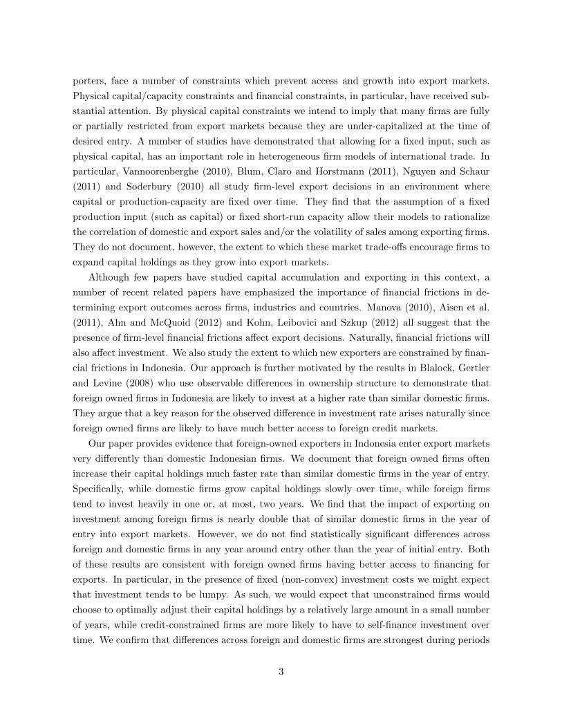
porters, face a number of constraints which prevent access and growth into export markets.

Physical capital/capacity constraints and financial constraints, in particular, have received sub-

stantial attention. By physical capital constraints we intend to imply that many firms are fully

or partially restricted from export markets because they are under-capitalized at the time of

desired entry. A number of studies have demonstrated that allowing for a fixed input, such as

physical capital, has an important role in heterogeneous firm models of international trade. In

particular, Vannoorenberghe (2010), Blum, Claro and Horstmann (2011), Nguyen and Schaur

(2011) and Soderbury (2010) all study firm-level export decisions in an environment where

capital or production-capacity are fixed over time. They find that the assumption of a fixed

production input (such as capital) or fixed short-run capacity allow their models to rationalize

the correlation of domestic and export sales and/or the volatility of sales among exporting firms.

They do not document, however, the extent to which these market trade-offs encourage firms to

expand capital holdings as they grow into export markets.

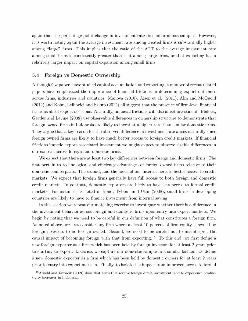
Although few papers have studied capital accumulation and exporting in this context, a

number of recent related papers have emphasized the importance of financial frictions in de-

termining export outcomes across firms, industries and countries. Manova (2010), Aisen et al.

(2011), Ahn and McQuoid (2012) and Kohn, Leibovici and Szkup (2012) all suggest that the

presence of firm-level financial frictions affect export decisions. Naturally, financial frictions will

also affect investment. We also study the extent to which new exporters are constrained by finan-

cial frictions in Indonesia. Our approach is further motivated by the results in Blalock, Gertler

and Levine (2008) who use observable differences in ownership structure to demonstrate that

foreign owned firms in Indonesia are likely to invest at a higher rate than similar domestic firms.

They argue that a key reason for the observed difference in investment rate arises naturally since

foreign owned firms are likely to have much better access to foreign credit markets.

Our paper provides evidence that foreign-owned exporters in Indonesia enter export markets

very differently than domestic Indonesian firms. We document that foreign owned firms often

increase their capital holdings much faster rate than similar domestic firms in the year of entry.

Specifically, while domestic firms grow capital holdings slowly over time, while foreign firms

tend to invest heavily in one or, at most, two years. We find that the impact of exporting on

investment among foreign firms is nearly double that of similar domestic firms in the year of

entry into export markets. However, we do not find statistically significant differences across

foreign and domestic firms in any year around entry other than the year of initial entry. Both

of these results are consistent with foreign owned firms having better access to financing for

exports. In particular, in the presence of fixed (non-convex) investment costs we might expect

that investment tends to be lumpy. As such, we would expect that unconstrained firms would

choose to optimally adjust their capital holdings by a relatively large amount in a small number

of years, while credit-constrained firms are more likely to have to self-finance investment over

time. We confirm that differences across foreign and domestic firms are strongest during periods

3

of tight domestic credit in Indonesia and indicative of impact of credit market imperfections on

export behavior.

Our results are not simply of academic interest, but have key policy implications, particularly

in a developing country. For instance, a large literature documents that changes in firm-level

investment behavior has important impacts on aggregate economic performance.4 Likewise,

Crucini and Kahn (1996, 2007) demonstrate that accounting for capital accumulation at an

aggregate level is key to evaluating trade policy changes. We complement this literature by

documenting similar differences in a developing country and studying the interaction of firm-

level investment with export decisions.

In the next section we provide a simple model of investment and exporting to motivate our

empirical approach. Section two describes our empirical strategy and section three describes the

Indonesian manufacturing sector and the data used to study firm-level investment and export

behavior. The fourth section presents our empirical model, while section five presents both our

main results and robustness checks. Section six examines the differential investment behavior

of new foreign and domestic exporters and the extent to which this can be attributed to credit

constraints. The last section concludes.

1 A Simple Model of Investment and Exporting

To facilitate our empirical analysis we present a simple model of investment and exporting. In

this model firms choose to increase their capital stock in order to grow into export markets. A

number of recent models argue that new exporters tend to be capacity constrained (Ahn and

McQuoid (2012), Soderbury (2010), Nguyen and Schaur (2012), Blum, Claro and Horstmann

(2011)) . In most of these models capital stock or firm capacity is exogenous to the decision to

export. In contrast, we present a stylized model in which investment and capital holdings en-

dogenously depend on the firm’s export decisions over time. Our objective here is to outline one

particular channel through which exporting may affect investment over time, though alternative

explanations should not be ruled out.

Consider a set horizontally differentiated manufacturings firm in a developing country which

each produce one variety which can be sold at home in the domestic market or abroad through ex-

port sales. Each firm produces according to a Cobb-Douglas production function qjt = eωjtkαkjt l

αljt

where q is the firm’s total production, ω is firm-specific productivity and k and l are the firm

j’s current holdings of capital and variable inputs, respectively. We assume that variable inputs

can be freely adjusted each period, but investment in physical capital only becomes productive

the year after the initial investment.

4For instance, Doms and Dunne (1998), Caballero, Engel and Haltiwanger (1995), Cooper, Haltiwanger andPower (1999) and Cooper and Haltiwanger (2000).

4

We can write firm j’s short-run marginal cost function as:

ln cjt = − lnαl −αkαl

ln kjt −1

αlωjt + lnwt +

1− αlαl

ln q∗jt (1)

where wt is a set of relevant input prices used in production and q∗jt is the target, profit-

maximizing level of output. Equation (1) implies that firms with larger capital stocks incur

lower marginal costs, ceteris paribus. This will later imply that across two equally productive

firms, the firm with the larger capital stock will produce at a lower cost. As such, more capital-

intensive firms will be more likely to export. We assume that productivity evolves according to

a separate Markov process:

ωjt = f(ωjt−1, kjt) + εjt (2)

where kjt captures the firm’s current holdings of capital. Likewise, we describe the evolution of

capital by

kjt = (1− δ)kjt−1 + ijt−1 (3)

where ijt−1 is the firm’s total investment in physical capital in period t−1 and δ is the per-period

depreciation rate on physical capital.

Firms also incur costs when they choose to invest or export. We write the firm’s investment

cost function, C(ijt, kjt), as

C(ijt, kjt) = c(ijt, kjt) + F1[ijt > 0] (4)

where c(0, kjt) = 0, c1 > 0, c2 < 0, c11 > 0, c22 > 0 and F captures the magnitude of fixed

investment costs.5 Similarly, we assume that entering foreign markets may require additional

fixed entry costs, CX(djt, djt−1), which may depend on the firm’s export history:

CX(djt, djt−1) = FXdjtdjt−1 + SXdjt(1− djt−1)

where djt takes a value of 1 if firm j exports in year t and is zero otherwise. If the initial entry

into export markets is more costly than subsequent entries into export markets we expect that

SX > FX .

We maintain standard assumptions regarding the structure of domestic and export markets

(see Melitz (2003) for an example). Both markets are assumed to be monopolistically com-

petitive, but segmented from each other so that firms will not interact strategically across

markets. The maximized profit function for firm j at time t (before investment costs) is:

5Both convex and non-convex parameters have been found to be important for capturing firm-level investmentdynamics in the US (c.f. Cooper and Haltiwanger (2006), Cooper, Haltiwanger and Willis (2010)) and Indonesia(c.f. Rho and Rodrigue (2012)).

5

πjt = πt(kit, ωjt, djt, djt−1, A,A∗) where A and A∗ capture market-specific demand shifters (size,

income, competitiveness) in the domestic and foreign market, respectively.

Denote the value of firm j in year t by Vjt:

Vjt(sjt) = maxdjt,ijt

πjt(sjt, djt)− C(ijt, kjt)− CX(djt, djt−1) + βEtVjt+1(sjt+1) (5)

where sjt = (kit, ωjt, djt, A,A∗) is a vector of state variables and

EtVjt+1(sjt+1) =

∫ω′Vjt+1(s′)dF (ω′|ωjt) (6)

If the firm does not choose to invest (ijt = 0), the firm’s capital stock will fall and the firm’s

marginal costs of production, for the same level of output, will rise next period. Conversely, if

the firm invests enough to increase its capital stock in period t+ 1 the firm’s marginal costs will

fall. The first-order condition for the investment decisions for either exporters and non-exporters

can be written as

c1(ijt, kjt) + F = βEt∂Vjt+1(sjt+1)

∂ijt(7)

The left side of (7) is the marginal cost of adjustment and is independent of the firm’s export

decision or history. The right side is the expected marginal gain and includes the effects on both

the intensive (the amount of investment) and extensive margins (whether to invest or not).6

This expected marginal gain from investment depends upon the firms export decision. First,

if entering export markets firms lowers the costs of future exporting, through sunk export costs

for example, firms will expect to produce and sell in a larger number of markets and to a

larger number of consumers. In our model this raises the marginal value of capital and in turn

encourages greater investment.

Similarly, the net benefit to exporting, conditional on the firm’s investment decision, can be

described by the value functions. We can write the marginal benefit from exporting, MBE, for

any firm as:

MBEjt = πjt(sjt, djt = 1)− πjt(sjt, djt = 0)− CX(djt, djt−1)︸︷︷︸Initial Gain/Loss

+βEtVjt+1(sjt+1, djt = 1)− Vjt+1(sjt+1, djt = 0)︸︷︷︸Future Gain/Loss

(8)

6The RHS of (7) ignores the effects of ijt on the probability of adjustment since the effect of capital adjustmenton the probability of adjustment is evaluated just at a point of indifference between adjusting and not adjusting.For each ijt there are values of ωjt which bound adjustment and non-adjustment. Variation in ijt does influencethese boundaries, but since the boundaries are points of indifference between adjustment and non-adjustment,there is no further effect on the value of the objective function. See Cooper, Haltiwanger and Willis (2010) forfurther discussion.

6

The marginal benefit to exporting captures both the current profits from exporting and

the expected future gains or losses from exporting. The initial gain captures the difference in

operating profits associated with exporting and any direct export entry costs. As emphasized

in recent literature, capital constrained exporters are likely to have relatively small gains in the

initial period of exporting since expansions into the export market may come at the cost of

lost domestic sales. At the same time, however, these constraints create a stronger incentive to

invest in the early years of exporting; not only do firms want to expand into export markets, but

they also want to be able to optimally serve the domestic market. As such, capital constrained

exporters may have large expected future gains from exporting since growth in capital holdings

may allow them to expand both at home and abroad.

2 Empirical Strategy

A primary concern for our empirical strategy is to address the endogeneity of the decision to

export on the estimated impact on investment. As a first step we choose to focus on firms

which enter export markets for the first time during the 1990-2000 period. Specifically, we

eliminate all plants which export during 1990 and/or 1991 to focus on the sample of initial non-

exporters. Consequently, we greatly reduce the number of firms under consideration. However,

by focussing on firms which are entering export markets for the first time we can then use

differencing over time to eliminate the influence of all observable and unobservable elements of

the export decision that are strongly persistent over time. Our strategy is to use a difference-

in-difference technique to compare the performance of new exporters with that of similar firms

who choose not to export. Naturally, the comparison is likely to suffer from non-random sample

selection since exporting firms endogenously choose to enter export markets. We use propensity

score matching, in combination with difference-in-difference methods, to address the selection

issue. The matching procedure controls for the selection of bias by restricting the comparison

to differences within carefully selected pairs of firms of firms who possess similar observable

characteristics. Specifically, each pair of firms consists of an exporting firm and a non-exporting

firm with similar characteristics two years preceding entry into export markets.

We choose to compare firms two years before entry for several reasons. First, as noted

by Rho and Rodrigue (2012) new exporters are likely to begin new investment before entering

export markets. Second, our method will allow us to trace out differences in investment behavior

through time by comparing investment performance before and after initial entry into export

markets. In particular, our aim is to measure the causal effect of exporting on the physical

investment rate, rt = itkt

, where it captures the current net investment rate (new investment

minus capital sales) and kt is the firm’s stock of capital in year t. Letting d = 1 for a new

7

exporter and 0 otherwise, this effect is defined as

E[rt(d = 1)− rt(d = 0)|d = 1] = E[rt(d = 1)|d = 1]− E[rt(d = 0)|d = 1]

which captures the difference between the performance paths of firms which started exporting

(the first term) and the performance paths of the same firms should they not have started ex-

porting (the second term). Clearly, we observe each firm as an exporter or non-exporter in

any year and never both, so that the second outcome is an unobserved counterfactual. The

objective of matching methods is to construct the missing counterfactual by drawing compar-

isons conditional on a vector of observable characteristics, X. It has been shown that as long

as relevant differences between two firms can be captured by the observable (pre-treatment)

variables, matching methods yield an unbiased estimate of the treatment impact (Dehejia and

Wahba, 2002). The key underlying assumption is that conditional on the observable character-

istics that are relevant for the export decision, potential outcomes for exporting (treated) and

non-exporting (untreated) are orthogonal to treatment status.

(rt(d = 1), rt(d = 0)) ⊥ d|X

The implication is that both firms of our matched pairs exhibit similar performance under

the same circumstances

E[rt(d = 1)− rt(d = 0)|d = 1] =[E[rt(d = 1)|X, d = 1]− E[rt(d = 0)|X, d = 0]

]−

[E[rt(d = 0)|X, d = 1]− E[rt(d = 0)|X, d = 0]

]=

[E[rt(d = 1)|X, d = 1]− E[rt(d = 0)|X, d = 0]

](9)

The second difference in equation (9) captures the selection bias. The key assumption in our

method is that this term is assumed to be zero conditional on X. It represents the difference

between the exporting firms, should they not have exported, and those that did not export,

in the same state (non-exporting). The first difference in equation (9) captures the causal

effect of exporting on physical investment. It follows that under the matching assumption the

performance difference between new exporters and non-exporting control observations is an

unbiased estimate of the causal effect.

In our setting, the propensity score is the predicted probability of entry into export markets.

Given the predicted probability of export entry we compare the performance of firms matched

on the basis of their propensity score. This technique is particularly attractive in this context as

there are a large number of observable variables with significant predictive power for determining

whether a firm will enter into export markets. Specifically, although our simple model provides

an intuitive and concise description of the firm’s investment and export decisions, we observe

(and document) that a wide set of observable firm-level characteristics have strong predictive

8

power even after controlling for observed firm-level productivity. Further, it is unclear how

to condition on a large number of variables when a priori we do not have a strong guide

on which dimensions firms should be matched. As noted by Rosenbaum and Rubin (1983)

propensity score matching provides a natural weighting scheme that yields unbiased estimates

of the treatment impact. Conditioning on the propensity score is equivalent to conditioning on

all of the available information, but reduces the dimensionality problem. Blundell and Costa

Dias (2000) highlight the benefits of combining matching with difference-in-difference methods

for controlling observable and unobservable differences between treatment and control units. In

particular, they emphasize that matching accounts for differences in observable characteristics

while difference-in-differences methods allows for an “unobserved determinant of participation

as long as it can be represented by separable individual and/or time-specific components of

the error term.” In our case, examples would include a particular firm entering export markets

because of its knowledge of foreign markets or the superior performance of the firm manager.

3 Data

The primary source of data is the Indonesian manufacturing census between 1990 and 2000.

Collected annually by the Central Bureau of Statistics, Budan Pusat Statistik (BPS), the survey

covers the population of manufacturing plants in Indonesia with at least 20 employees. The data

capture the formal manufacturing sector and record detailed plant-level information on over 100

variables covering industrial classification (5-digit ISIC), revenues, capital stock, new investment

in physical capital, capital sales, intermediate inputs, exports, and ownership structure. Data

on revenues and inputs are deflated with wholesale price indices.7

Key to our analysis the data also include a measure of the market value of capital holdings

along with the value of new investment in each year except 1996. Specifically, the data contain

annual observations on the estimated value of fixed capital, new investment and capital sales

across five type types of capital: land, buildings, vehicles, machinery and equipment, and other

capital not classified elsewhere. The capital stock and investment series are created by aggregat-

ing data across types. Following Blalock and Gertler (2004) we deflate capital using a wholesale

price indices for construction, imported electrical and non-electrical equipment and imported

transportation equipment. To construct the capital stock deflator we weight each price index by

the average reported shares of buildings and land, machinery and equipment and fixed vehicle

assets.8

7Price deflators are constructed as closely as possible to Blalock and Gertler (2004) and include separatedeflators (1) output and domestic intermediates, (2) energy, (3) imported intermediates and (4) export sales.

8Our measure of capital has several advantages. First, using a market value of capital the measure accountsfor variation in depreciation and changes in the productivity of the current capital stock across firms. We observethat, like other data sets that provide direct estimates of depreciation (e.g. Schundeln, 2011), this value variessubstantially in the cross-section, particularly in particularly in developing countries. Second, we observe thatacross industries there is large cross-sectional variation in the degree to which firms invest in physical capital that

9

Table 1: Investment and Export Moments

VariableAverage investment rate (I/K) 0.052Inaction frequency 0.714Fraction of observations with negative investment 0.013Average export intensity 0.092Export frequency 0.133Correlation of export and investment status 0.169Correlation of log export sales and log investment 0.534

3.1 Investment and Export Moments

The main features of the investment and export sales distributions are summarized in Table 1.

We omit any firms for which there is missing investment and capital information. In 1990, there

are 13,641 manufacturing plants that contain a full set of information, while by 2000 the data

covers 18,211 plants.

First, note that 71.4 percent of the (firm-year) observations report no new investment or

capital sales and only 1.3 percent report any capital sales. This suggests that in only 27.3

percent of observations do we observe positive net investment. Moreover, only 13.9 percent of

firms report investment rates greater than 11 percent, the average reported depreciation rate in

the sample.

The investment rate and frequency documented in Table 1 are somewhat lower than those

reported in the US (Cooper and Haltiwanger, 2006), Norway (Nilsen and Schiantarelli, 2003)

and even Columbia (Huggett and Ospina, 2001). This can largely be attributed to the fact that

in each of the above papers, the authors study a balanced panel of manufacturing firms, whereas

we keep all of the firms in our sample. Balancing our panel of manufacturing firms results in

significant data loss during the 1997-1998 Asian crisis. If we examine comparable moments for

a balanced sample in the pre-crisis period (1990-1995) we find an average investment rate of

10.9 percent, an inaction frequency of 63.9, and a positive investment frequency of 34.9 percent.

Moreover, 17.4 percent of firms demonstrate new investment greater than 11 percent. These

figures are closer to those found elsewhere, but continue to reflect the more stringent investment

environment in Indonesia relative to the US or Norway.

On average 13 percent of firms export in the sample while the average percentage of sales

is not classified in one of the four main classes of capital. To the extent that the nature of this capital variesacross firms we might expect that the temporal variation in its productivity, market value and depreciation tobe an additional source of variation over time not otherwise captured. Third, the data has excellent coverageacross firms. It is often difficult to get reliable estimates of firm-level capital holdings in developing countries,particularly in cases where small firms do not have accurate recording of the book value of capital. Alternatively,we also construct a capital series for each firm using perpetual inventory methods. This results in a distributionof capital across firms which is nearly identical to that from our preferred measure of capital. We do, however,have to drop numerous firms from the data set because of missing investment data from year to year. As such, wepresent results from the first measure of capital here. We have checked our results using the measure of capitalconstructed by perpetual inventory and find very similar estimates.

10

from exports is just more than 9 percent. As is typical in many firm-level manufacturing data

sets, export revenues are often small compared to the domestic market. The last two rows

examine the correlation between exporting and investment. We observe current export and

investment status are positively correlated, but the correlation coefficient is just below 0.17. If

we restrict our attention to firms that are both investing and exporting in the same year, we

observe that the correlation coefficient on the log of export sales and the log of net investment

rises to 0.53.

3.2 Estimating Productivity

As suggested by our model, total factor productivity is a key variable in our analysis since firm-

level export and investment decisions are typically strongly correlated with measures of firm-level

efficiency. We measure total factor productivity using a multilateral index developed by Caves

et al. (1982) and Aw, Chen and Roberts (2001). The key advantage of this index is that it allows

for consistent comparisons of TFP in firm-level panel data.9 The idea underlying the index is

that each firm’s productivity is measured relative to a single reference point. Specifically, the

index compares firm j’s inputs (capital, labor, materials, energy) and output in year t to a

hypothetical reference firm operating in the base time period (t = 0) with average input cost

shares, average log inputs and average log output:

lnTFPjt = (lnYjt − lnYt) +t∑

τ=2

(lnYτ − lnYτ−1)

−

[n∑

m=1

1

2(Sjmt + Smt)(lnXjmt − lnXmt)

+t∑

τ=2

n∑m=1

1

2(Smτ − Smτ−1)(lnXmτ − lnXmτ−1)

]

where m indexes the type of input. As noted above output Y is measured in real terms along

with inputs, X: labor (the number of employees), materials (real value of materials costs),

energy (real value of electricity and fuel) and capital. S captures input shares for each input

other than capital. For example, the labor share is measured as the ratio of the real wage bill

to output. The capital share is obtained by assuming constant returns to scale. Finally, X, Y

9Van Biesebroeck (2007) compares the robustness of five commonly used measures of productivity (indexnumbers, data envelopment, stochastic frontier, GMM and semi-parametric estimation). He finds that the indexnumber approach taken here tends to produce very robust results. Arnold and Javorcik (2011) similarly computefirm-level productivity on a similar set of Indonesian firms and report that this measure is strongly robust intheir sample. Nonetheless, for robustness, we have also estimated a productivity series for each firm following themethods described in Olley and Pakes (1996) and applied to this data set as in Amiti and Konings (2007). Wecould not reject the hypothesis of constant returns to scale in any industry. Since the results from the matchingexercise were very similar in all cases we have omitted them from the main text.

11

and S are the inputs, output and input shares of the hypothetical reference plant.

3.3 Export Premia

We document investment behavior across three different groups of firms: incumbent exporters,

new exporters and non-exporters. We define an incumbent exporter as a firm which had positive

export sales in years t − 1 and t while new exporters, in contrast, capture firms that did not

export in t− 1. Non-exporters capture the remaining firms which did not export in the current

year.

While Table 2 suggests that exporting has a strong positive impact on investment it is not

clear that these differences are significant or causal. To approach these issues we first consider a

simple regression of the firm’s investment rate on it’s export status. We measure the investment

rate, rjt = ijt/kjt, as the firm j’s net investment ijt, new investment less capital sales, in year t

divided by the existing capital stock, kjt.10

rjt = β0 + βxxjtxjt−1 + βnxjt(1− xjt−1) + εjt (10)

where xjt ∈ {0, 1} is a binary variable which takes a value of one if the firm exports in year t and

εjt is an error term. While our specification is purposefully simple, the estimated coefficients are

an easily interpretable measure of the size and significance of the relationship between exporting

and investment.

The first row of Table 2 presents OLS estimates of coefficients from equation (10). In

each case we include province, year and industry (ISIC 4-digit) dummies. The first column

restricts the coefficients across incumbent and new exporters to be identical and suggests that

the investment rate among exporters is 5.1 higher than non-exporting firms. While this is a

moderate increase in the investment rate, it represents a drastic change in investment behavior.

The average investment rate among exporting firms is 0.110. As such, the export premium for

exporters, 0.051, represents nearly half of new investment among new exporters during the year

of entry. Column (2) allows the export premium to vary across new and existing exporters. We

observe very similar results; the export premium among new exporters is 4.7 percentage points,

while it is 4.8 percentage points among incumbent exporters.

Columns (3)-(14) repeat the experiment for numerous subsamples and different dimensions

in our data. Specifically, we separately examine the investment in machinery (columns 3-4),

investment among domestic (columns 5-6) and foreign firms (columns 7-8), investment before

(columns 9-10) and after the Asian crisis (columns 11-12), and among small firms (columns

13-14). Remarkably, we observe nearly identical, strongly significant export premia in each

10Alternatively, we considered the log of new investment as our dependent variable. While it yielded similarresults, it’s use required dropping many firms in our sample because the firm chose not to invest or was reducingits capital holdings. Moreover, we would be unable to perform analysis over time since only a small portion ofour sample invests continuously over time.

12

Tab

le2:

Inve

stm

ent

Rat

ean

dE

xp

orti

ng

Tota

lIn

v.

inD

om

est

icFore

ign

Pre

-Cri

sis

Cri

sis/

Post

-Cri

sis

Sm

all

Invest

ment

Machin

ery

Fir

ms

Fir

ms

1991-1

996

1997-2

000

Fir

ms

OL

Sre

gre

ssio

ns

wit

hin

dust

ry,

pro

vin

ce

and

year

fixed

eff

ects

All

Exp

ort

ers

0.0

51***

0.0

58***

0.0

43***

0.0

46***

0.0

51***

0.0

49***

0.0

60***

(0.0

02)

(0.0

03)

(0.0

02)

(0.0

07)

(0.0

03)

(0.0

03)

(0.0

05)

Incum

bent

Exp

ort

ers

0.0

48***

0.0

53***

0.0

40***

0.0

36***

0.0

48***

0.0

46***

0.0

63***

(0.0

03)

(0.0

04)

(0.0

03)

(0.0

09)

(0.0

04)

(0.0

04)

(0.0

09)

New

Exp

ort

ers

0.0

47***

0.0

57***

0.0

40***

0.0

50***

0.0

42***

0.0

49***

0.0

36***

(0.0

03)

(0.0

04)

(0.0

03)

(0.0

08)

(0.0

04)

(0.0

03)

(0.0

06)

R-s

quare

d0.0

38

0.0

34

0.0

38

0.0

37

0.0

33

0.0

29

0.0

82

0.0

80

0.0

39

0.0

37

0.0

33

0.0

31

0.0

31

0.0

27

No.

of

obs.

150,4

77

121,6

48

119,5

98

96,6

31

142,3

96

114,8

15

8,0

81

6,8

33

84,1

77

60,4

12

66,3

00

61,2

36

72,2

65

56,1

19

Regre

ssio

ns

wit

hfi

rmand

year

fixed

eff

ects

All

Exp

ort

ers

0.0

15***

-0.0

04

0.0

10***

0.0

47***

0.0

04

0.0

19***

0.0

11**

(0.0

03)

(0.0

04)

(0.0

03)

(0.0

08)

(0.0

04)

(0.0

04)

(0.0

06)

Incum

bent

Exp

ort

ers

0.0

13***

-0.0

04

0.0

08**

0.0

38***

0.0

08

0.0

11**

0.0

04

(0.0

03)

(0.0

04)

(0.0

03)

(0.0

10)

(0.0

05)

(0.0

05)

(0.0

09)

New

Exp

ort

ers

0.0

17***

0.0

08**

0.0

14***

0.0

47***

0.0

08

0.0

21***

0.0

10*

(0.0

03)

(0.0

04)

(0.0

03)

(0.0

10)

(0.0

05)

(0.0

04)

(0.0

06)

R-s

quare

d0.0

19

0.0

12

0.0

13

0.0

06

0.0

17

0.0

11

0.0

65

0.0

48

0.0

12

0.0

05

0.0

09

0.0

06

0.0

16

0.0

05

No.

of

obs.

144,7

21

118,0

18

113,5

66

92,4

38

136,4

79

111,0

55

7,6

08

6,4

89

77,8

99

57,4

53

63,1

79

58,1

54

24,1

82

20,5

81

OL

Sre

gre

ssio

ns

wit

hin

dust

ry,

pro

vin

ce

and

year

fixed

eff

ects

Incum

bent

Exp

ort

ers

0.0

11***

0.0

20***

0.0

10***

0.0

26***

0.0

09**

0.0

14***

0.0

10***

(>3

years

post

entr

y)

(0.0

02)

(0.0

03)

(0.0

02)

(0.0

08)

(0.0

04)

(0.0

02)

(0.0

04)

New

Exp

ort

ers

0.0

28***

0.0

32***

0.0

23***

0.0

47***

0.0

17***

0.0

34***

0.0

21***

(Years

1-

3)

(0.0

02)

(0.0

03)

(0.0

02)

(0.0

07)

(0.0

04)

(0.0

02)

(0.0

03)

R-s

quare

d0.0

32

0.0

36

0.0

28

0.0

91

0.0

32

0.0

35

0.0

34

No.

of

obs.

97,4

49

73,3

63

91,5

60

5,8

89

31,1

49

66,3

00

48,6

56

Note

s:R

ob

ust

stan

dard

erro

rs,

clu

ster

edat

the

firm

-lev

el,

are

inp

are

nth

eses

.∗∗∗,∗∗

,∗

ind

icate

sign

ifica

nce

at

the

1%

,5%

,an

d10%

level

s,re

spec

tivel

y.

13

case. Further, the OLS regressions reveal little discernible difference across new and incumbent

exporters.

Although these initial results are striking, there are a number of alternative explanations

for the statistically significant relationship between exporting and investment. For instance,

our estimates likely reflect unobserved differences across firms. As our model suggests more

productive firms are likely to invest at a higher rate. Similarly, we might expect that new

exporters may adjust capital holdings over numerous years and, as such, our definitions of new

and incumbent exporters may be misleading. We take a first pass at addressing these concerns

in the bottom two panels.

In the second panel we re-estimate equation (10) with firm-level fixed effects. In this case

the export premia coefficients are identified solely by within-firm variation. Moreover, to the

extent that key firm-level differences, such as productivity, are persistent over time, we expect

that the firm-level fixed effects will at least partially control for these factors. Across all columns

the export premia coefficients are now estimated to be substantially smaller, though in most

cases strongly significant. In the full sample, we find that exporters invest 1.5 percent faster

than non-exporters overall. Although this coefficient is small, it represents 14 percent of overall

investment among exporting firms.

The second panel also reveals small, but important differences across new and incumbent

exporters. In particular, the point estimates of the export premia among new exporters tend to

be larger and more strongly significant than those among incumbent exporters. This is to be

expected since new exporters are likely to be smaller, more capital constrained and likely have

had less time to adjust capital holdings. For a limited set of firms and industries Rodrigue and

Rho (2012) suggest that new exporters are likely begin investing at a faster rate in the years

preceding first entry and continue investing at a faster rate for at least 2 years after entry. In

our case, our estimates so far only capture the immediate impact of exporting on investment.

In the last panel, we redefine a new exporter as an exporter which has begun exporting in the

past 3 years while an incumbent exporter is an exporter with at least 3 years of experience in

export markets. Again we observe that both new and incumbent exporters tend to invest at a

higher rate than non-exporting firms. However, we now observe larger differences between new

and incumbent exporters.

A particularly striking result is that from foreign owned firms (column 8).11 We observe that

in each panel foreign-owned exporting firms tend to invest much more heavily than other foreign

-owned non-exporters. New investment in developing countries is often plagued by numerous

financial frictions and, as such, new financing can be difficult to secure.12 Differences in access

11We define a foreign firm as one where at least 10 percent of equity is held by foreign investors.12Blalock, Gertler and Levine (2008) exploit these ownership differences across firms in Indonesia to measure

how access to world financial markets affected the evolution of new physical investment during the Asian crisis.In particular, they examine differential investment rates across similar foreign and domestic firms to measure therole of credit access on investment.

14

to credit markets may be reflected in the observed investment rates; better access to credit

may allow foreign firms the ability to adjust capital holdings to new export opportunities. In

particular, if domestic firms have to finance a larger portion of investment through internal

saving we might expect that new domestic exporters adjust by smaller amounts over a longer

time period relative to foreign firms. Alternatively, the difference might simply reflect large

differences in firm-level productivity, which are not adequately controlled for in our simple

regressions. We examine these issues, among others, below.

4 An Empirical Model of Exporting and Investment

Our objective is to study the paths of investment before and after entry into export markets. In

order to implement propensity score matching we need an empirical model for the entry of firms

into export markets. We begin by estimating a probit model of the binary decision to enter

export markets. In general, the logarithm of observable plant-level characteristics are lagged

two years and pertain to the pre-entry period. We believe that observable characteristics are a

reasonable starting point since firm-level capabilities in terms of productivity, size, employment,

capital or skill-intensity are likely to influence the extent to firms are able and willing to easily

enter export markets. Further, we observe detailed firm-level information which characterizes

the degree to which non-exporting firms are integrated in world markets, either through foreign

ownership or imported intermediate inputs.

We choose to use variables which are lagged two years because we believe that future ex-

porters are likely to begin increasing investment in physical capital prior to initial entry. Specif-

ically, our working assumption is that export related investment begins at earliest one year prior

to entry so that variables lagged two years are fully part of the pre-entry period. This assumption

is consistent with the related findings in Lopez (2009) and Rho and Rodrigue (2012). However,

we will relax this assumption in our robustness checks.

The results are presented in Table 3. We observe that the exporting firms differ strongly

from non-exporters. In particular, firms with greater TFP and its square are more likely to

enter export markets; the coefficients on TFP is significant at standard levels. Further, younger,

larger (in terms of employment) and more capital intensive firms are more likely to export. Firms

which are already internationally integrated, either by sourcing foreign inputs or having foreign

ownership, are also much more likely to enter export markets. We are particularly interested

in the large coefficient on lagged foreign ownership. If entry into new markets requires costly

investments, we might expect that foreign owned firms - which are likely to benefit from access for

foreign credit markets - may be better able to become successful exporters. These are consistent

with prior literature and our initial expectations. We have also included the net investment

rate lagged two periods to ensure that matches assigned on the basis of propensity score will be

homogeneous with respect to previous investment behavior. This is particularly important in

15

our case since this helps control for any plants which begin accumulating capital in anticipation

of future entry into export markets.

The only variable which is insignificant in Table 3 is the average wage. Our hypothesis

is that average wage, as suggested by Fox and Smeets (2011), is strongly correlated with the

average skill-level among employees. This variable, and its square turns out to be statistically

insignificant. There are three natural reasons to expect this result. First, there may be little

independent variation in this measure which is not already captured by the other explanatory

variables. Second, skill-intensity may not a key determinant of exporting in a developing coun-

try such as Indonesia, whose comparative advantage may in less-skilled, labor-intensive goods.

Third, the average wage may be a poor measure of skill in this country. To check this last

possibility we replaced the average wage with ratio of non-production to production employees

in each firm and repeated the probit exercise. We found nearly identical results on all coeffi-

cients; in particular, the coefficient on the skill-ratio, and its square, were again estimated to be

insignificantly different from zero.

The predicted probability of exporting resulting from the model in Table 3 will form the

propensity score and act as the metric for our matching procedure. We use one-to-one nearest

neighbor matching.13 We restrict that any two matched firms must be chosen from the same

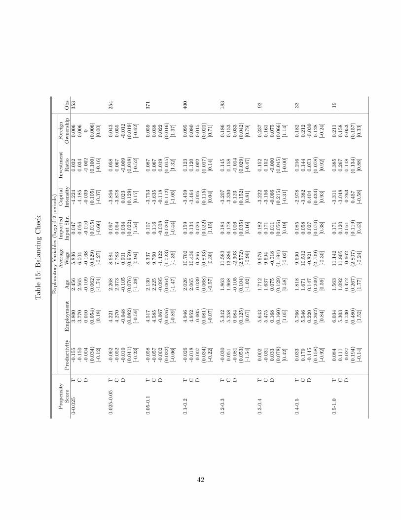
year and industry. To determine how successful our matching procedure is we compare the

difference between the treated and control group in terms of each of the above variables and

compute t-statitics for each of the reported variables across 8 bands of the propensity score.

In no case do we find statistically significant differences.14 In the full sample, our matched

pairs of firms are only one percentage point apart in terms of propensity score. This suggests

that our matches are very close along this measure and we can have confidence in the resulting

comparisons.15 Finally, in all of specifications below, we find that results suggest no statistically

significant differences in the investment rates across treated and control firms in the pre-sample

period.

5 Results

5.1 Full Sample

We first examine the difference-in-difference results on the full sample of matched firms. We

observe in Table 4 that the matching procedure appears to work very well; two years before entry

there is less 1.5 percentage point difference in the estimated investment rates between treated

13We have repeated our experiment using alternative matching strategies such as increasing the number ofcontrol matches (10), local linear regression matching, spline matching and full Mahalanobis matching. Since themain results are almost identical across matching strategies we do not present further results below.

14This exercise is often referred to as the balancing hypothesis (see Dehejia and Wahba, 2002). The results ofthis exercise are presented in the Appendix.

15Recall, that the propensity score measure is bounded by 0 and 100.

16

Table 3: Probit: Predicting Export EntryTFPt−2 0.171***

(0.019)TFP2

t−2 0.039*(0.022)

Employmentt−2 0.941***(0.043)

Employment2t−2 -0.059***

(0.004)Age -0.387***

(0.034)Age2 0.043***

(0.007)Capital per Workert−2 0.103***

(0.016)Capital per Worker2

t−2 0.002(0.002)

Average Waget−2 0.001(0.001)

Average Wage2t−2 -0.00002

(0.00004)Imported Input Sharet−2 0.450***

(0.120)Imported Input Share2

t−2 -0.356***(0.131)

Investment Ratiot−2 0.421***(0.114)

Investment Ratio2t−2 -0.351***

(0.134)Foreign Ownershipt−2 0.311***

(0.030)Export Statust−2 1.255***

(0.025)Time Trend 0.024***

(0.004)

No. of obs. 80,500Chi2 21,841.67Prob > Chi2 0.000Pseudo R2 0.395

Notes: Four-digit industry dummies, province dummies and year dummies are included but not reported. ∗ ∗ ∗, ∗∗, ∗indicate significance at the 1%, 5%, and 10% levels, respectively.

17

−2 −1 0 1 20.04

0.05

0.06

0.07

0.08

0.09

0.1

0.11A

vera

ge Investm

ent R

ate

Time

T

C

−2 −1 0 1 2−0.01

0

0.01

0.02

0.03

0.04

0.05

0.06

AT

T

Time

ATT95% Bootstrap C .I .

and control firms. Moreover, we observe that the difference in the propensity score is very small.

However, although both treatment and control groups begin with similar investment rates, they

diverge quickly. In particular, we observe that exporting firms maintain high investment rates

during the entry period while the non-exporting control group observe investment rates that

decline sharply over the same period. This pattern reflects the lumpiness of investment. New

exporters are likely to be firms which are investing heavily before entry. Not surprisingly the

matched control firms demonstrate similar investment behavior in the initial period. However,

among exporters it is reasonable to expect that it will take several years to expand into export

markets; in developing countries where access to credit is relatively we might expect that capital

accumulation is stretched out over time since many firms have to finance capital expenditures

internally. As such, it is not surprising that investment rates remain high among the treated

group. In contrast, among non-exporting firms, investment is likely to capture the normal

replacement of depreciated capital. Since these firms are not expanding into new markets it

is reasonable that these investments would occur over a much-shorter time period among non-

exporting firms.

The estimated investment rates are plotted graphically in Figure 1. We observe that the

difference in between investment rates between the treated and control groups grows during the

year before entry and into the initial entry period. The year after entry the difference between

investment rates shrinks, even though the investment rate among exporting firms remains signifi-

cantly higher than that of non-exporting firms. The difference between rates then grows slightly,

on average, two years after initial entry. This reflects the fact that exporting affects not only

the level of investment in physical capital, but also the timing of investment. Exporting firms

are more likely to invest more heavily in consecutive years as they grow into export markets.

In contrast, non-exporting firms have less incentive to continue investing heavily in consecutive

years since they are generally responding to domestic shocks alone and replacing depreciated

capital.

18

Table 4: Investment Rate and Exporting, Full SampleTwo Years One Year Year of One Year Two Years

Before Entry Before Entry(a) Entry(b) Later(c) Later(d)

Treatment Group: T 0.101 0.099 0.090 0.067 0.068Control Group: C 0.086 0.069 0.054 0.051 0.049ATT 0.015 0.030*** 0.037*** 0.016*** 0.019***

(0.009) (0.009) (0.009) (0.006) (0.007)

ATT/T 0.303 0.411 0.239 0.279No. of matched pairs 1,801 1,512 1,598 1,338 1,003Mean difference in 0.013 0.014 0.013 0.014 0.017propensity score

Notes: The first two lines present the outcomes observed in the given time period. The average treatment effect on the

treated (ATT) is presented in the third row along with bootstrapped standard errors in parentheses. ∗ ∗ ∗, ∗∗, ∗ indicate

significance at the 1%, 5%, and 10% levels, respectively.

(a) ATT = 1n

∑n1

[(ik

)treatedentry year−1

−(ik

)control

entry year−1

]− 1

n

∑n1

[(ik


−(ik

)control

entry year−2

](b) ATT = 1

n

∑n1

[(ik

)treatedentry year+0

−(ik

)control

entry year+0

]− 1

n

∑n1

[(ik


−(ik

)control

entry year−2

](c) ATT = 1

n

∑n1

[(ik


−(ik

)control

entry year+1

]− 1

n

∑n1

[(ik


−(ik

)control

entry year−2

](d) ATT = 1

n

∑n1

[(ik


−(ik

)control

entry year+2

]− 1

n

∑n1

[(ik


−(ik

)control

entry year−2

]

The window immediately around entry suggests that the difference in investment rates rise

with exporting. The average treatment effect on the treated (ATT) suggests that average in-

vestment rate spikes up by 3 percentage points in the year preceding entry, 4 percentage points

year of entry and 2 percentage points in the two years after entry among treated firms. These

are all strongly significant at conventional levels and represent large increases in investment

behavior. Although the percentage point differences are small it is important to remember that

the average investment, even among exporting firms, is typically quite low. To get a sense of the

relative change in investment behavior, we calculate the relative export effect as the ratio of the

average treatment effect on the treated to mean investment rate among the treated firms in each

year. We observe that relative to the average investment rate among treated firms, the average

treatment effects on the treated suggesting that exporting accounts for a very large percentage

of total investment; among treated firms exporting roughly accounts for 24 to 41 percent of total

investment between the year before entry and two years afterwards.

Our results suggest that upon entry into export markets large firm-level changes, particularly

in the physical composition and organization of the firms, are well underway. This clearly affects

the interpretation of numerous results in the literature. For instance, Ahn and McQuoid (2012),

Vannoorenberghe (2012), Nguyen and Schaur (2011) and Soderbury (2010) suggest that new

exporters are often restricted in their entry into export markets by physical capacity constraints.

Our results suggest that these constraints are likely to alleviated within a small number of years

since exporting firms are actively expanding capital stock. Further, physical capital constants

have been suggested as a mechanism through which export market shocks are transmitted to the

19

domestic market. Our results suggest that if firms are actively accumulating capital to optimally

serve both home and export markets the severity of this transmission mechanism should decline

over time.

The reader will notice that the number of matched pairs varies over time. This occurs for two

reasons. First, the survey does not collect investment information in 1996. This differentially

affects the number of matches which are missing information in any two years; that is, the

number of firms missing information for year t = −1 is different than that in year t = 0 and so

on. Second, some firms endogenously exit our sample. To the extent that smaller, non-exporting

firms are more likely to exit and less likely to invest, we might expect that the estimated ATT is

downwards biased. Likewise, our main sample combines the effects across all types of ownership

structure, size and time periods. This last effect is of particular concern in this context since it

well known that Indonesia suffered a strong contraction during and after the onset of the Asian

crisis in 1997. We consider these issues in our robustness checks.

5.2 Asian Crisis

One of the features of sample is that it covers the period in which Indonesia was subject to the

Asian financial crisis. The Asian financial crisis began in the fall of 1997 and continued well into

1998. There are two features of the Asian which are of particular interest in our study. First,

the onset of the financial crisis was widely reported to have sharply restricted access to credit

during the crisis years. Moreover, although the Indonesian economy had begun to recover by

1999, access to credit continued to be much more restricted in comparison the pre-crisis period

(Ito and Sato, 2006). Second, it is well known that aggregate exports fell substantially during

this period.

To the extent that the Asian crisis may have affected firm-level exporting and investment

rates, we may expect that our estimates may be biased. What is less clear, however, is the direc-

tion of the bias. On one hand, smaller export opportunities and tighter investment regulation

are likely to reduce investment and discourage large entries into export markets. As such, we

might expect that our estimates in the full sample could be biased towards zero if the Asian

crisis is not adequately controlled for in the full sample. On the other hand, if only the strongest

firms are able to export during the Asian crisis we might expect that these exporting firms are

very productive and have a particularly strong incentive to invest.

We investigate this possibility by repeating our exercise before the Asian crisis period (1990-

1996) and on the period during and after the Asian crisis (1997-2000). Comparing the top

and bottom panels of Table 5 we immediately observe a number of key differences across time

periods. In particular, the mean investment rates among both treated and control firms are

much higher before the crisis relative to the subsequent crisis period. Further, we also observe

a stronger impact on investment behavior prior to entering export markets in the pre-sample

20

Table 5: Investment Rate and Exporting, Asian Financial CrisisPre-Crisis (1991-1995)

Two Years One Year Year of One Year Two Years


Treatment Group: T 0.121 0.112 0.102 0.079 0.072Control Group: C 0.099 0.080 0.072 0.069 0.055ATT 0.021 0.032*** 0.030*** 0.010 0.017*

(0.014) (0.011) (0.011) (0.010) (0.010)

ATT/T 0.286 0.294 0.127 0.236No. of matched pairs 881 871 881 663 597Mean difference in 0.013 0.013 0.013 0.014 0.018propensity score

Crisis and Post-Crisis (1997-2000)



Treatment Group: T 0.079 0.070 0.076 0.049 0.044Control Group: C 0.066 0.052 0.027 0.030 0.023ATT 0.013 0.019 0.049*** 0.019* 0.021*

(0.010) (0.012) (0.008) (0.010) (0.012)




significance at the 1%, 5%, and 10% levels, respectively. Investment data is not collected in 1996.

(a) ATT = 1n

∑n1

[(ik


−(ik

)control

entry year−1

]− 1

n

∑n1

[(ik


−(ik

)control

entry year−2

](b) ATT = 1

n

∑n1

[(ik


−(ik

)control

entry year+0

]− 1

n

∑n1

[(ik


−(ik

)control

entry year−2

](c) ATT = 1

n

∑n1

[(ik


−(ik

)control

entry year+1

]− 1

n

∑n1

[(ik


−(ik

)control

entry year−2

](d) ATT = 1

n

∑n1

[(ik


−(ik

)control

entry year+2

]− 1

n

∑n1

[(ik


−(ik

)control

entry year−2

]

21

period, while during the crisis period exporting appears to have a stronger impact on investment

rates after entry. This would be consistent with the notion that firms had less access to credit

markets during the period and had to self-finance a greater portion of investment from their

own sales, creating a delay in total investment. Likewise, the results may be indicative of

greater uncertainty in both domestic and exports influencing the timing of investment. Last,

although the percentage point difference between exporting and non-exporting firms is smaller

during the crisis period, this does not necessarily imply that the relative effect of exporting

was smaller over the same time. Rather, we observe that exporting accounts for nearly twice

as much of total investment after initial entry into export markets during the crisis period; for

example, the ATT/T × 100 ≈ 30% in year of entry during the pre-crisis period, while this same

calculation jumps to 65% during the crisis period. Our results strongly suggest as the domestic

market contracted sharply during the Asian crisis, export markets were a particularly important

determinant of investment behavior among exporting firms.16

5.3 Small vs. Large Firms

In this section we investigate differences across firm size. In particular, we are interested in the

extent to which the incentive to increase capital holdings differs across large and small firms.

We expect that we may observe differences along this dimension for a number of reasons. On

one hand, by virtue of being small, small firms may have a greater need to increase capacity as

they enter export markets. On the other hand, large firms may have be able to secure cheaper

financing and, as such, expand more rapidly into export markets.

How to distinguish large firms with access to credit markets from smaller, less-connected

counterparts is unclear. We begin with a simple definition of large firms: we define a large firm

in the Indonesian manufacturing sector as one with more than 100 employees two years before

initial entry into export markets.17 This roughly divides the sample in two equally sized groups

in Table 6. We observe that exporting appears to have an impact on investment among both

groups of firms, though the ATT suggests that it may be moderately stronger among smaller

firms.

To test the robustness of these findings we consider a second definition of firm size. In

particular, we calculate the median capital stock in each 4-digit industry. Then we define a

“large firm” as any firm which has at least as much capital as the median firm in the industry

two years prior to first entry into export markets. The results are presented in Table 7. We find

16The reader will notice the large change in the number of matches over time. This relates to the sampleconstruction issues highlighted in section 6.1 which are exacerbated during the crisis period. First, there are veryfew new exporters in 1998, the trough year of the Asian crisis, which greatly reduces the number of matches inadjacent years. Second, the rate of firm exit is substantially higher during this period. As noted, above we willstudy these issues in detail below.

17Our definition is similar to that in Blalock, Gertler and Levine (2008), who study a similar set of Indonesianmanufacturing firms.

22

Table 6: Investment Rate Across Large and Small Firms (Employment)Large Firms (Employment ≥ 100)



Treatment Group: T 0.128 0.121 0.106 0.081 0.088Control Group: C 0.120 0.104 0.076 0.067 0.069ATT 0.009 0.018 0.029** 0.014 0.019*

(0.015) (0.011) (0.012) (0.010) (0.011)


Small Firms (Employment < 100)



Treatment Group: Tp 0.077 0.080 0.076 0.054 0.048Control Group: C 0.072 0.052 0.046 0.044 0.032ATT 0.006 0.028*** 0.030*** 0.010 0.015

(0.009) (0.008) (0.007) (0.008) (0.011)





(a) ATT = 1n

∑n1

[(ik


−(ik

)control

entry year−1

]− 1

n

∑n1

[(ik


−(ik

)control

entry year−2

](b) ATT = 1

n

∑n1

[(ik


−(ik

)control

entry year+0

]− 1

n

∑n1

[(ik


−(ik

)control

entry year−2

](c) ATT = 1

n

∑n1

[(ik


−(ik

)control

entry year+1

]− 1

n

∑n1

[(ik


−(ik

)control

entry year−2

](d) ATT = 1

n

∑n1

[(ik


−(ik

)control

entry year+2

]− 1

n

∑n1

[(ik


−(ik

)control

entry year−2

]

23

Table 7: Investment Rate Across Large and Small Firms (Capital)Large Firms (K ≥ K)



Treatment Group: T 0.115 0.102 0.099 0.078 0.081Control Group: C 0.096 0.079 0.062 0.064 0.064ATT 0.018 0.024** 0.037*** 0.013 0.016

(0.013) (0.011) (0.011) (0.009) (0.012)

ATT/T 0.235 0.374 0.176 0.198No. of matched pairs 1,027 895 890 772 570Mean difference in 0.007 0.008 0.007 0.007 0.008propensity score

Small Firms (K < K)



Treatment Group: T 0.062 0.071 0.066 0.044 0.042Control Group: C 0.059 0.051 0.037 0.034 0.018ATT 0.003 0.020 0.029*** 0.010 0.024**

(0.011) (0.012) (0.009) (0.009) (0.011)





(a) ATT = 1n

∑n1

[(ik


−(ik

)control

entry year−1

]− 1

n

∑n1

[(ik


−(ik

)control

entry year−2

](b) ATT = 1

n

∑n1

[(ik


−(ik

)control

entry year+0

]− 1

n

∑n1

[(ik


−(ik

)control

entry year−2

](c) ATT = 1

n

∑n1

[(ik


−(ik

)control

entry year+1

]− 1

n

∑n1

[(ik


−(ik

)control

entry year−2

](d) ATT = 1

n

∑n1

[(ik


−(ik

)control

entry year+2

]− 1

n

∑n1

[(ik


−(ik

)control

entry year−2

]

24

again that the percentage point change in investment rates is similar across samples. However,

it is worth noting again the average investment rate among treated firms is substantially higher

among “large” firms. This implies that the ratio of the ATT to the average investment rate

among small firms is consistently greater than that among large firms, or that exporting has a

relatively larger impact on capital expansion among small firms.

5.4 Foreign vs Domestic Ownership

Although few papers have studied capital accumulation and exporting, a number of recent related

papers have emphasized the importance of financial frictions in determining export outcomes

across firms, industries and countries. Manova (2010), Aisen et al. (2011), Ahn and McQuoid

(2012) and Kohn, Leibovici and Szkup (2012) all suggest that the presence of firm-level financial

frictions affect export decisions. Naturally, financial frictions will also affect investment. Blalock,

Gertler and Levine (2008) use observable differences in ownership structure to demonstrate that

foreign owned firms in Indonesia are likely to invest at a higher rate than similar domestic firms.

They argue that a key reason for the observed difference in investment rate arises naturally since

foreign owned firms are likely to have much better access to foreign credit markets. If financial

frictions impede export-associated investment we might expect to observe sizable differences in

our context across foreign and domestic firms.

We expect that there are at least two key differences between foreign and domestic firms. The

first pertain to technological and efficiency advantages of foreign owned firms relative to their

domestic counterparts. The second, and the focus of our interest here, is better access to credit

markets. We expect that foreign firms generally have full access to both foreign and domestic

credit markets. In contrast, domestic exporters are likely to have less access to formal credit

markets. For instance, as noted in Bond, Tybout and Utar (2008), small firms in developing

countries are likely to have to finance investment from internal saving.

In this section we repeat our matching exercise to investigate whether there is a difference in

the investment behavior across foreign and domestic firms upon entry into export markets. We

begin by noting that we need to be careful in our definition of what constitutes a foreign firm.

As noted above, we first consider any firm where at least 10 percent of firm equity is owned by

foreign investors to be foreign owned. Second, we need to be careful not to misinterpret the

causal impact of becoming foreign with that from exporting.18 To this end, we first define a

new foreign exporter as a firm which has been held by foreign investors for at least 2 years prior

to starting to export. Likewise, we capture our domestic sample in a similar fashion; we define

a new domestic exporter as a firm which has been held by domestic owners for at least 2 years

prior to entry into export markets. Finally, to isolate the impact from improved access to formal

18Arnold and Javorcik (2009) show that firms that receive foreign direct investment tend to experience produc-tivity increases in Indonesia.

25

Table 8: Investment Rate and Exporting, Foreign vs. Domestic FirmsForeign Firms



Treatment Group: T 0.124 0.130 0.130 0.097 0.125Control Group: C 0.174 0.140 0.066 0.058 0.101ATT -0.049 -0.010 0.064** 0.038** 0.024

(0.036) (0.043) (0.0315) (0.019) (0.041)

ATT/T -0.077 0.492 0.392 0.197No. of matched pairs 122 116 105 86 57Mean difference in 0.019 0.020 0.019 0.023 0.023propensity score

Domestic Firms



Treatment Group: T 0.095 0.092 0.082 0.060 0.066Control Group: C 0.076 0.061 0.052 0.045 0.043ATT 0.016 0.031*** 0.030*** 0.015** 0.022**

(0.010) (0.010) (0.010) (0.007) (0.009)

ATT/T 0.337 0.366 0.250 0.333No. of matched pairs 1,510 1,258 1,348 1,133 857Mean difference in 0.006 0.006 0.006 0.006 0.005propensity score




(a) ATT = 1n

∑n1

[(ik


−(ik

)control

entry year−1

]− 1

n

∑n1

[(ik


−(ik

)control

entry year−2

](b) ATT = 1

n

∑n1

[(ik


−(ik

)control

entry year+0

]− 1

n

∑n1

[(ik


−(ik

)control

entry year−2

](c) ATT = 1

n

∑n1

[(ik


−(ik

)control

entry year+1

]− 1

n

∑n1

[(ik


−(ik

)control

entry year−2

](d) ATT = 1

n

∑n1

[(ik


−(ik

)control

entry year+2

]− 1

n

∑n1

[(ik


−(ik

)control

entry year−2

]

credit markets we exploit our matching technique in order to match new exporters with similar

non-exporting firms with the same initial productivity levels.

The results from this exercise are presented in Table 8. We observe immediately that the

estimated average treatment effects on the treated are generally more significant among domestic

firms rather than foreign firms in the window around entry into export markets. The most

notable exception is the very large ATT among foreign exporters in the year they enter export

markets. In this year, the ATT captures a 6.4 percentage point increase in the investment rate

among foreign exporters and is strongly significant. Moreover, when we compare the ATT in

the year of entry relative to the average investment rate among foreign exporters we find that

it explains nearly one half of total firm-level investment.

The results from the sample of domestic firms contrast sharply. First, we note that we begin

to observe significant differences between treated and control firms in the year before initial

26

entry and these continue during the year of entry and for two years after entry. This result is

consistent with the idea that domestic firms may be constrained by financial frictions and, as

such, can only adjust capital holdings slowly over time. We find that the investment rate among

domestic exporters is 3.1 percentage points higher in the year before entry, 3.0 percentage points

higher in the year of entry and 1.5 and 2.2 percentage points higher in the two years after entry.

Collectively, these explain approximately one quarter to one third of overall investment in each

year.

The results from Table 8 are suggestive of financial frictions affecting firm-level entry into

export markets. However, we should interpret them cautiously. In particular, the control firms

are likely to differ substantially across subsamples and, as such, it would be incorrect to draw

conclusions by comparing the estimated differences between treated and control groups across

experiments. Nonetheless, these findings motivate further inquiry into the impact of financial

frictions on firm-level export and investment behavior. We return to study this issue in more

detail in Section 6.

5.5 Disaggregated Investment

Our data allows us to disaggregate each firm’s capital stock and investment into a number of sub-

categories. To get a sense of the nature of firm-level capital expansion during entry into export

markets we repeat our matching exercise for three groups of capital holdings: machinery and

equipment, buildings and land, and vehicles. Because the data for the individual components

of investment tends to be much more volatile than that of total investment we trim the bottom

and top one percent of each disaggregated investment before performing our analysis.

Among total capital holdings in our data set machinery and equipment, buildings and land,

and vehicles account for nearly 19, 41, and 8 percent of recorded holdings, respectively. Likewise,

among investing firms machinery and equipment, buildings and land, and vehicles account for

nearly 40, 26, and 18 percent of new investment, respectively.19 Our expectation is that the

increase in the firm’s productive capacity associated with entry into export markets is most

closely associated with the holdings of the physical machinery and equipment necessary for

production.

The results for machinery and equipment, buildings and land, and vehicles are presented

in Table 9. As expected we observe highly significant results for investment in machinery and

equipment both in the year preceding initial entry and in the year of initial entry, while the

ATT is only marginally significant in the year after first entry. The point estimates suggest

that investment rate for machinery is 3.6, 5.1 and 2.3 percentage points the years immediately

around initial entry. Relative to the average investment rate across firms, these estimates imply

a 27-44 percent increase in machinery investment over those 3 years.

19The remaining investment, capital sales or capital stock is classified as “other investment not classified else-where.”

27

Table 9: Investment Rate and Exporting, Disaggregated InvestmentMachinery and Equipment



Treatment Group: T 0.115 0.116 0.116 0.084 0.080Control Group: C 0.099 0.0.081 0.065 0.061 0.064ATT 0.016 0.036** 0.051*** 0.023* 0.017

(0.015) (0.015) (0.014) (0.014) (0.018)


Buildings and Land



Treatment Group: T 0.072 0.073 0.060 0.044 0.048Control Group: C 0.054 0.038 0.040 0.031 0.035ATT 0.018 0.035*** 0.021** 0.013 0.013

(0.012) (0.012) (0.010) (0.011) (0.013)


Vehicles



Treatment Group: T 0.127 0.126 0.130 0.094 0.093Control Group: C 0.131 0.078 0.082 0.074 0.074ATT -0.004 0.048** 0.049*** 0.019 0.019

(0.016) (0.021) (0.016) (0.016) (0.020)





(a) ATT = 1n

∑n1

[(ik


−(ik

)control

entry year−1

]− 1

n

∑n1

[(ik


−(ik

)control

entry year−2

](b) ATT = 1

n

∑n1

[(ik


−(ik

)control

entry year+0

]− 1

n

∑n1

[(ik


−(ik

)control

entry year−2

](c) ATT = 1

n

∑n1

[(ik


−(ik

)control

entry year+1

]− 1

n

∑n1

[(ik


−(ik

)control

entry year−2

](d) ATT = 1

n

∑n1

[(ik


−(ik

)control

entry year+2

]− 1

n

∑n1

[(ik


−(ik

)control

entry year−2

]

28

Table 10: Investment Rate and Exporting, Early Investing Robustness Check

Three Years Two Years One Year Year of One Year Two Years

Before Entry Before Entry Before Entry(a) Entry(b) Later(c) Later(d)

Treatment Group 0.089 0.071 0.083 0.077 0.061 0.064Control Group 0.089 0.075 0.061 0.041 0.052 0.039ATT 0.000 -0.004 0.022** 0.035*** 0.008 0.025**

(0.011) (0.010) (0.011) (0.010) (0.009) (0.010)

ATT/T -0.056 0.265 0.455 0.131 0.391No. of matched pairs 949 946 736 796 625 588Mean difference in 0.010 0.010 0.012 0.009 0.011 0.012propensity score




(a) ATT = 1n

∑n1

[(ik


−(ik

)control

entry year−1

]− 1

n

∑n1

[(ik


−(ik

)control

entry year−2

](b) ATT = 1

n

∑n1

[(ik


−(ik

)control

entry year+0

]− 1

n

∑n1

[(ik


−(ik

)control

entry year−2

](c) ATT = 1

n

∑n1

[(ik


−(ik

)control

entry year+1

]− 1

n

∑n1

[(ik


−(ik

)control

entry year−2

](d) ATT = 1

n

∑n1

[(ik


−(ik

)control

entry year+2

]− 1

n

∑n1

[(ik


−(ik

)control

entry year−2

]

Somewhat surprisingly, we observe similar, significant increases in vehicles and buildings and

land in both the year preceding initial entry and the year of initial entry into export markets. In

particular, the impact of exporting on investment relative to the average investment rate among

exporting firms would suggest that exporting has similar across all types of capital holdings.

5.6 Early Investing

In all our specifications we match firms based on their characteristics two years prior to entry.

Although this is line with previous research (e.g. Lopez (2009) or Rho and Rodrigue (2012)), it

is possible that firms begin accumulating capital more than one year in advance of initial entry

into export markets. To investigate this possibility we repeat the above experiment for earlier

years. Specifically, we first repeat the probit exercise only using firm-level characteristics which

are observable 3-years prior to entry. While this will allow us to study a longer pre-entry period

it also has the effect of greatly reducing our sample. We will now only be able to include firms

which have existed for at least three years prior to initial entry in our exercise. Nonetheless, we

repeat our first stage probit exercise using variables lagged three periods to form a propensity

score and proceed to match firms based on this new metric.20 The results from the matching

exercise are presented in Table 10.

When we match firms based on characteristics three years prior to entry, we observe no

statistical difference in the investment rate across firms two or three years prior to entry. As in

20Results from the probit regression can be found in the Appendix.

29

our previous specifications we do observe larger differences one year prior to entry and up to two

years afterwards. Although most estimates of the average treatment effect on the treated are

slightly smaller than our preferred estimates, they do remain strongly statistically significant.

Nonetheless, we do not find any evidence that firms begin investing more than one year prior to

entry. Because of this we choose to focus on the results from our preferred specification where

we use firm-characteristics two years prior to entry to match firms.

5.7 Sample Selection

Another potential concern is that our estimates will be broadly affected by sample attrition.

We examine this issue by studying samples of firms which are in our sample for at least T years

where T = 6, 7, 8. Specifically, the treated sample includes firms which exist for at least 2 years

before entering export markets and T − 3 years after entry (not including the year of entry).

The group of control firms include firms which exist T years but never export. The results from

the matching exercise are presented in Table 11.

Naturally, as we impose stronger requirements on the length of time a firm must be present,

our overall sample size falls. Despite the reduction in sample size in all cases we find very

similar results to those found in the full sample both in size and significance. Moreover, we now

generally find average treatment effects 2-3 percentage points, which are strongly significant

results beyond a year after initial entry into export markets. In the bottom panel of Table 11 we

report the results for our strictest time requirement; we required that firms produce for at least

8 consecutive years. Although we again find nearly identical results before entry and during

the initial year of entry, our estimates after entry lose statistical significance. There are at least

three interpretations for this last finding. First, long-lived firms may have better relationships

with lending institutions and are able to fully adjust capital holdings within a smaller number

of years. As such, we may not expect to find strongly significant results beyond one or years

after initial entry. Second, our requirement that firms produce for at least 8 years results in

a substantial reduction in our matched sample size. This in and of itself may be responsible

for the reduction in statistical significance. Last, it well known that many new exporters only

continue to export for a small number of years after first entry. We examine this issue next.

5.8 Endogenous Exit from Export Markets

As often reported, many new exporters do not export for many consecutive years (see Eaton et al.

(2009), Arkolakis (2010) and Rho and Rodrigue (2012) for examples). A potential concern in our

context is that new exporters which exit export markets shortly after entry may have a smaller

incentive to invest and, as such, bias our main estimates. We examine this issue by repeating

our experiment on subsamples of firms which have different export histories. Specifically, we

restrict the treated sample to new exporting firms which export for at least 2 consecutive years.

30

Tab

le11

:In

vest

men

tR

ate

and

Exp

orti

ng,

Fir

ms

wh

ich

pro

du

cefo

rT

con

secu

tive

year

sF

irm

sw

hic

hpro

duce

for

6co

nse

cuti

ve

yea

rs

Tw

oY

ears

One

Yea

rY

ear

of

One

Yea

rT

wo

Yea

rsT

hre

eY

ears

Bef

ore

Entr

yB

efore

Entr

yE

ntr

yL

ate

rL

ate

rL

ate

r

Tre

atm

ent

Gro

up

0.1

09

0.1

21

0.0

97

0.0

74

0.0

71

0.0

64

Contr

ol

Gro

up

0.0

94

0.0

83

0.0

62

0.0

64

0.0

51

0.0

43

ATT

0.0

15

0.038

***

0.035

***

0.011

0.020

**

0.021

***

(0.0

10)

(0.0

13)

(0.0

10)

(0.0

07)

(0.0

08)

(0.0

07)

AT

T/T

0.314

0.361

0.149

0.282

0.328

No.

of

matc

hed

pair

s1,0

98

887

927

953

946

926

Mea

ndiff

eren

cein

0.0

17

0.0

19

0.0

16

0.0

17

0.0

17

0.0

17

pro

pen

sity

score

Fir

ms

whic

hpro

duce

for

7co

nse

cuti

ve

yea

rs

Tw

oY

ears

One

Yea

rY

ear

of

One

Yea

rT

wo

Yea

rsT

hre

eY

ears

Four

Yea

rsB

efore

Entr

yB

efore

Entr

yE

ntr

yL

ate

rL

ate

rL

ate

rL

ate

r

Tre

atm

ent

Gro

up

0.1

24

0.1

22

0.1

10

0.0

82

0.0

77

0.0

75

0.0

52

Contr

ol

Gro

up

0.1

12

0.0

93

0.0

80

0.0

75

0.0

62

0.0

53

0.0

46

ATT

0.0

12

0.029

**

0.030

***

0.022

**

0.016

0.023

*0.006

(0.0

11)

(0.0

13)

(0.0

10)

(0.0

10)

(0.0

09)

(0.0

12)

(0.0

10)

AT

T/T

0.238

0.273

0.268

0.208

0.306

0.115

No.

of

matc

hed

pair

s836

836

671

699

692

679

603

Mea

ndiff

eren

cein

0.0

20

0.0

20

0.0

20

0.0

22

0.0

21

0.0

21

0.0

16

pro

pen

sity

score

Fir

ms

whic

hpro

duce

for

8co

nse

cuti

ve

yea

rs

Tw

oY

ears

One

Yea

rY

ear

of

One

Yea

rT

wo

Yea

rsT

hre

eY

ears

Four

Yea

rsF

ive

Yea

rsB

efore

Entr

yB

efore

Entr

yE

ntr

yL

ate

rL

ate

rL

ate

rL

ate

rL

ate

r

Tre

atm

ent

Gro

up

0.1

33

0.1

25

0.1

10

0.0

84

0.0

76

0.0

84

0.0

54

0.0

55

Contr

ol

Gro

up

0.1

16

0.0

99

0.0

81

0.0

86

0.0

60

0.0

53

0.0

45

0.0

53

ATT

0.0

17

0.026

**

0.028

**

0-.002

0.016

0.031

**

0.009

0.002

(0.0

14)

(0.0

12)

(0.0

11)

(0.0

11)

(0.0

11)

(0.0

12)

(0.0

11)

(0.0

10)

AT

T/T

0.208

0.255

-0.023

0.211

0.369

0.167

0.036

No.

of

matc

hed

pair

s640

640

640

509

498

491

422

640

Mea

ndiff

eren

cein

0.0

21

0.0

21

0.0

21

0.0

22

0.0

23

0.0

23

0.0

16

0.0

21

pro

pen

sity

score

Note

s:T

he

firs

ttw

olin

esp

rese

nt

the

ou

tcom

esob

serv

edin

the

giv

enti

me

per

iod

.T

he

aver

age

trea

tmen

teff

ect

on

the

trea

ted

(AT

T)

isp

rese

nte

din

the

thir

dro

walo

ng

wit

hb

oots

trap

ped

stan

dard

erro

rsin

pare

nth

eses

.∗∗∗,∗∗

,∗

ind

icate

sign

ifica

nce

at

the

1%

,5%

,an

d10%

level

s,re

spec

tivel

y.T

he

AT

Tis

com

pu

ted

an

alo

gou

sly

toth

at

inoth

erta

ble

s(t

he

form

ula

sare

sup

pre

ssed

for

ease

of

pre

senta

tion

.

31

Table 12: Investment Rate and Exporting, ≥ 2 Years of Consecutive ExportingTwo Years One Year Year of One Year Two Years


Treatment Group 0.116 0.109 0.100 0.072 0.084Control Group 0.102 0.085 0.073 0.054 0.065ATT 0.014 0.024** 0.027** 0.018** 0.019

(0.010) (0.012) (0.011) (0.008) (0.013)





(a) ATT = 1n

∑n1

[(ik


−(ik

)control

entry year−1

]− 1

n

∑n1

[(ik


−(ik

)control

entry year−2

](b) ATT = 1

n

∑n1

[(ik


−(ik

)control

entry year+0

]− 1

n

∑n1

[(ik


−(ik

)control

entry year−2

](c) ATT = 1

n

∑n1

[(ik


−(ik

)control

entry year+1

]− 1

n

∑n1

[(ik


−(ik

)control

entry year−2

](d) ATT = 1

n

∑n1

[(ik


−(ik

)control

entry year+2

]− 1

n

∑n1

[(ik


−(ik

)control

entry year−2

]

As expected our restriction results in a substantial reduction in sample size. However, we

again observe nearly identical results. In Table 12 we consider the set of new exporters which

export for at least two years in a row. The average treatment effect on the treated estimates

suggest that the investment rate is 2-3 percentage points higher in the years immediately around

initial entry. Relative to the full sample we find that the export effect accounts for a slightly

smaller percentage of total investment. This is can largely be attributed to the fact that the

average investment among our continuing exporters is higher than the average investment rate

in the full sample both before and after entry. This is not surprising given that the continuing

exporters are generally among the largest and most productive firms in each industry.

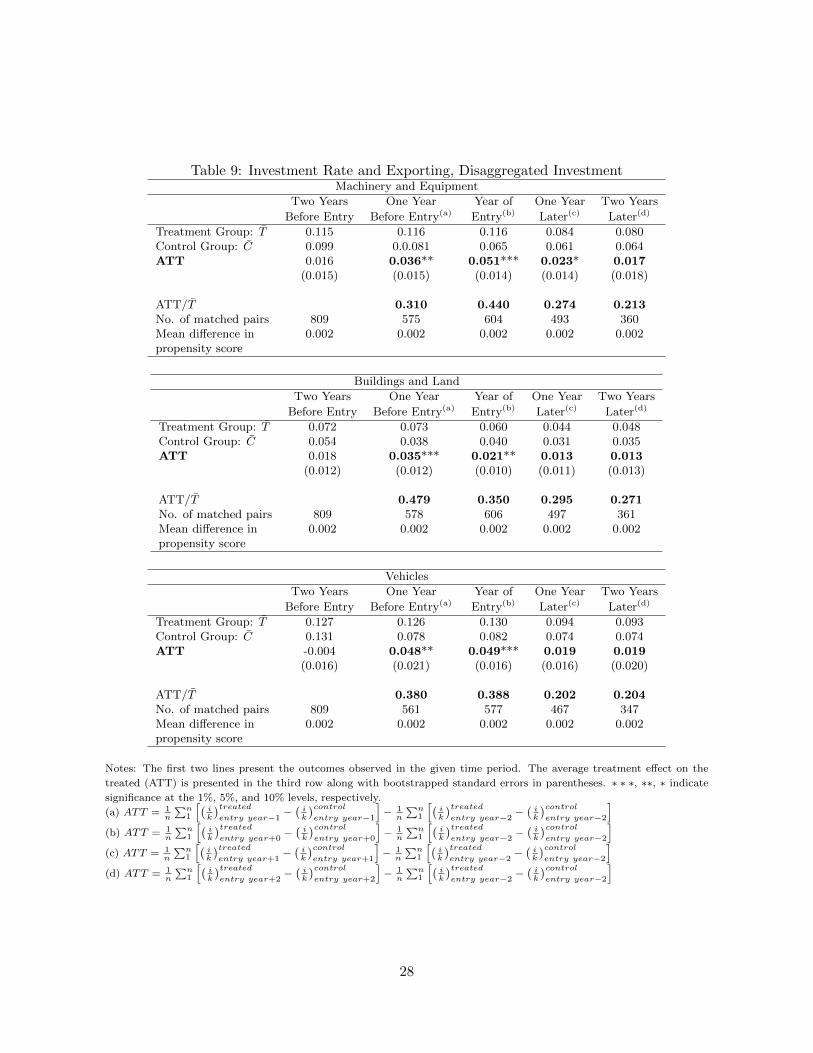
6 Foreign and Domestic Firms Revisted

In this section we revisit our examination of the differential impact exporting has on investment

across domestic and foreign-owned firms. Previously we saw that exporting had a significant

impact on investment rate among both foreign and domestic exporters in separate experiments.

Our matching exercise, however, did not allow for a straightforward comparison of the rela-

tive magnitude of these effects for a number of reasons. First, we also observe similarly large

differences in the standard errors on the average treatment effects in Table 8. This is hardly

surprising: our definition of a foreign firm greatly reduces the number of foreign firms in our

sample and, consequently, inflates the standard errors on that group of firms. Second, the av-

erage investment rate across foreign and domestic firms also varies considerably among control

32

firms.

To address this issue we consider a second experiment in the same spirit as our preceding

matching exercise. We first regress the investment rate in year t+l on dummy variables capturing

the firm export and ownership status and a large set of control variables where l = −1, 0, 1, 2.

The idea is to capture differences in firm-level investment rates across foreign and domestic firms

in comparison to a given set of control firms.

Specifically, the variable xdjt takes a value of 1 if a domestic firm is a first-time exporter

in year t and 0 otherwise. Likewise, the variable xfjt similarly takes a value of 1 if the firm

is simultaneously a first time exporter in year t and owned by foreign investors.21 Finally, we

also include a large number of controls for firm-level characteristics, lagged two periods, on the

right-hand side. This leads us to consider the following regression

rj,t+l = α0 + αdxdjt + αfx

fjt + βXj,t−2 + ujt (11)

where Xj,t−2 includes firm-level measures of productivity, employment, age, capital-intensity,

average wages, imported input shares, investment ratio and the square of each of these inde-

pendent variables. Importantly, we also include the firm’s ownership status as an explanatory

variable. This implies that αf will capture the impact of exporting on investment above and

beyond any investment premium that pertains to foreign firms in and of themselves.

This simple regression allows us to test a number of interesting results. First, by testing

the difference between αf and αd, we can test whether there are significant differences in the

impact exporting has on the investment rate across similar foreign and domestically-owned

firms. Second, we are able to document evidence of the impact of financial frictions affecting

export behavior in Indonesia. Specifically, our previous exercise suggested a number of empirical

patterns which would be consistent with the presence of financial frictions. We expect that the

domestic export premium αd will be positive and significant in numerous years surrounding

initial entry into export markets. To the extent that domestic firms have to self-finance new

investment we expect that they may not be able to fully adjust capital holdings in one year if

they face significant financial constraints. In contrast, we expect that foreign exporters will have

a positive export premium αf in only one or at most two years around export entry. Since foreign

firms are likely to have better access to foreign credit markets we believe that they will be better

able to finance to new investment in a shorter-period of time and grow into export markets

quickly. Further, since we are comparing firms with very similar firm-level characteristics we

expect that in the years immediately around entry into export markets we will observe a positive

difference between the foreign and domestic export premia, αf −αd > 0. In this case, a positive

and significant difference would represent evidence of underinvestment by domestic firms.

21Our definition of a foreign firm is as before. For a firm to be considered foreign at least 10 percent of equitymust be held by foreign investors continuously over the pre-entry and entry period.

33

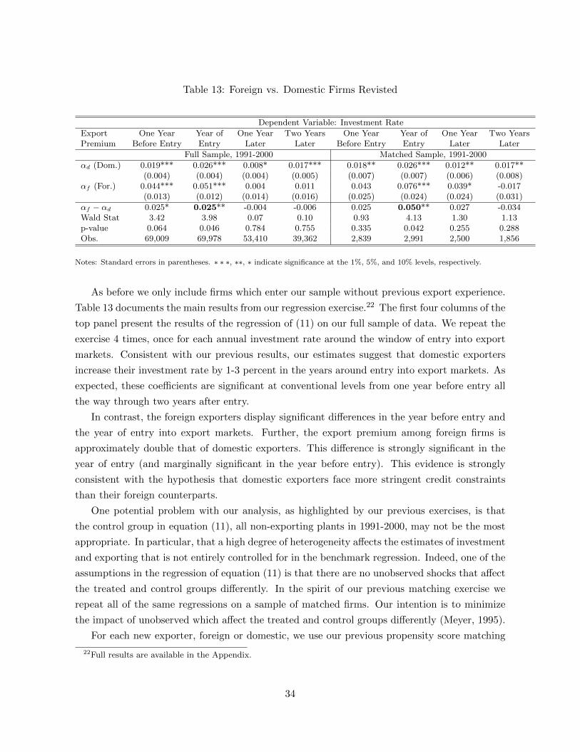
Table 13: Foreign vs. Domestic Firms Revisted

Dependent Variable: Investment Rate

Export One Year Year of One Year Two Years One Year Year of One Year Two YearsPremium Before Entry Entry Later Later Before Entry Entry Later Later

Full Sample, 1991-2000 Matched Sample, 1991-2000

αd (Dom.) 0.019*** 0.026*** 0.008* 0.017*** 0.018** 0.026*** 0.012** 0.017**(0.004) (0.004) (0.004) (0.005) (0.007) (0.007) (0.006) (0.008)

αf (For.) 0.044*** 0.051*** 0.004 0.011 0.043 0.076*** 0.039* -0.017(0.013) (0.012) (0.014) (0.016) (0.025) (0.024) (0.024) (0.031)

αf − αd 0.025* 0.025** -0.004 -0.006 0.025 0.050** 0.027 -0.034Wald Stat 3.42 3.98 0.07 0.10 0.93 4.13 1.30 1.13p-value 0.064 0.046 0.784 0.755 0.335 0.042 0.255 0.288Obs. 69,009 69,978 53,410 39,362 2,839 2,991 2,500 1,856

Notes: Standard errors in parentheses. ∗ ∗ ∗, ∗∗, ∗ indicate significance at the 1%, 5%, and 10% levels, respectively.

As before we only include firms which enter our sample without previous export experience.

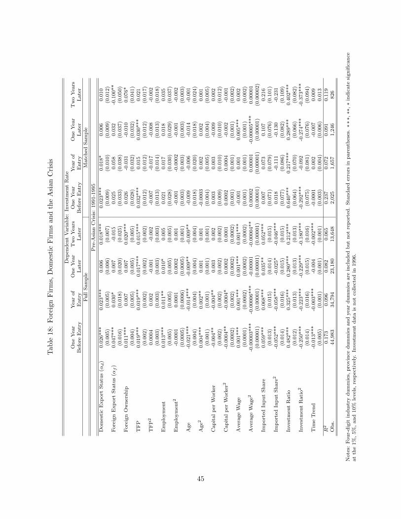
Table 13 documents the main results from our regression exercise.22 The first four columns of the

top panel present the results of the regression of (11) on our full sample of data. We repeat the

exercise 4 times, once for each annual investment rate around the window of entry into export

markets. Consistent with our previous results, our estimates suggest that domestic exporters

increase their investment rate by 1-3 percent in the years around entry into export markets. As

expected, these coefficients are significant at conventional levels from one year before entry all

the way through two years after entry.

In contrast, the foreign exporters display significant differences in the year before entry and

the year of entry into export markets. Further, the export premium among foreign firms is

approximately double that of domestic exporters. This difference is strongly significant in the

year of entry (and marginally significant in the year before entry). This evidence is strongly

consistent with the hypothesis that domestic exporters face more stringent credit constraints

than their foreign counterparts.

One potential problem with our analysis, as highlighted by our previous exercises, is that

the control group in equation (11), all non-exporting plants in 1991-2000, may not be the most

appropriate. In particular, that a high degree of heterogeneity affects the estimates of investment

and exporting that is not entirely controlled for in the benchmark regression. Indeed, one of the

assumptions in the regression of equation (11) is that there are no unobserved shocks that affect

the treated and control groups differently. In the spirit of our previous matching exercise we

repeat all of the same regressions on a sample of matched firms. Our intention is to minimize

the impact of unobserved which affect the treated and control groups differently (Meyer, 1995).

For each new exporter, foreign or domestic, we use our previous propensity score matching

22Full results are available in the Appendix.

34

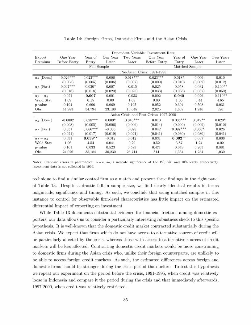
Table 14: Foreign Firms, Domestic Firms and the Asian Crisis

Dependent Variable: Investment RateExport One Year Year of One Year Two Years One Year Year of One Year Two YearsPremium Before Entry Entry Later Later Before Entry Entry Later Later

Full Sample Matched Sample

Pre-Asian Crisis: 1991-1995

αd (Dom.) 0.026*** 0.023*** 0.006 0.018*** 0.023*** 0.018* 0.006 0.010(0.005) (0.005) (0.006) (0.007) (0.009) (0.010) (0.009) (0.012)

αf (For.) 0.047*** 0.030* 0.007 -0.015 0.025 0.058 0.032 -0.100**(0.016) (0.018) (0.020) (0.025) (0.033) (0.038) (0.037) (0.050)

αf − αd 0.021 0.007 0.001 -0.033 0.002 0.040 0.026 -0.110**Wald Stat 1.69 0.15 0.00 1.68 0.00 1.06 0.44 4.65p-value 0.194 0.696 0.969 0.195 0.952 0.304 0.508 0.031Obs. 44,983 34,794 23,180 13,648 2,025 1,657 1,246 826

Asian Crisis and Post-Crisis: 1997-2000

αd (Dom.) -0.0002 0.028*** 0.009* 0.016*** 0.010 0.035*** 0.019** 0.020*(0.008) (0.005) (0.006) (0.006) (0.014) (0.009) (0.009) (0.010)

αf (For.) 0.031 0.066*** -0.003 0.028 0.042 0.097*** 0.056* 0.026(0.021) (0.017) (0.019) (0.021) (0.041) (0.030) (0.030) (0.041)

αf − αd 0.031 0.038** -0.012 0.012 0.031 0.062** 0.037 0.006Wald Stat 1.96 4.54 0.041 0.29 0.52 3.87 1.24 0.02p-value 0.161 0.033 0.523 0.589 0.471 0.049 0.265 0.881Obs. 24,026 35,184 30,230 25,714 814 1,334 1,254 1,030

Notes: Standard errors in parentheses. ∗ ∗ ∗, ∗∗, ∗ indicate significance at the 1%, 5%, and 10% levels, respectively.

Investment data is not collected in 1996.

technique to find a similar control firm as a match and present these findings in the right panel

of Table 13. Despite a drastic fall in sample size, we find nearly identical results in terms

magnitude, significance and timing. As such, we conclude that using matched samples in this

instance to control for observable firm-level characteristics has little impact on the estimated

differential impact of exporting on investment.

While Table 13 documents substantial evidence for financial frictions among domestic ex-

porters, our data allows us to consider a particularly interesting robustness check to this specific

hypothesis. It is well-known that the domestic credit market contracted substantially during the

Asian crisis. We expect that firms which do not have access to alternative sources of credit will

be particularly affected by the crisis, whereas those with access to alternative sources of credit

markets will be less affected. Contracting domestic credit markets would be more constraining

to domestic firms during the Asian crisis who, unlike their foreign counterparts, are unlikely to

be able to access foreign credit markets. As such, the estimated differences across foreign and

domestic firms should be stronger during the crisis period than before. To test this hypothesis

we repeat our experiment on the period before the crisis, 1991-1995, when credit was relatively

loose in Indonesia and compare it the period during the crisis and that immediately afterwards,

1997-2000, when credit was relatively restricted.

35

The top panel of Table 14 documents the estimated regression coefficients in both the full

and matched samples before the Asian crisis, while the bottom panel presents the same results

for the period afterwards when credit was relatively tight. In the pre-crisis period we observe

coefficients of similar magnitude to those in the full-sample, though the statistical significance is

somewhat reduced. Most importantly, we do not observe any statistically significant differences

across foreign and domestic firms. Although the coefficients on the foreign exporter dummy are

generally larger than their domestic counterparts, these differences are relatively small and are

insignificantly different from zero in all years around entry into export markets.

We contrast these results with those from the bottom panel. The magnitude of the coefficients

on the export dummies increase among both domestic and foreign exporters and are generally

more significant. This potentially reflects the growing importance of the export market in a

period when the domestic market is contracting. Further, the difference between the foreign

exporter effect αf and the domestic exporter effect αd only grows by small amount in every

year, except the year of initial entry into exports markets. In the year of entry foreign firms

we observe significant differences between similar foreign and domestic exporters. It is striking

that this difference, highlighted in the Table 13, disappears in the pre-crisis period, but shows

up relatively strongly during the crisis period when credit is tight. This is strongly consistent

with the view that new domestic exporters are face binding credit constraints as they grow into

export markets.

7 Conclusion

This paper documents the extent to which firm-level capital accumulation grows when Indonesian

firms enter export markets. We contribute to this literature by quantifying the degree to which

new exporters increase capital holdings at a faster rate upon entering export markets. Our

model suggests that if new exporters are constrained by a lack of physical capital at the time

of entry into export markets, exporting will encourage investment in new capital among those

firms that wish to grow into export markets.

Our findings suggest that firms adjust to exporting over a number of years. We find that new

exporters begin investing at a faster rate one year before entry and a higher rate of investment

continues into the year of entry and for two years after entry (for a total of at least 4 years). In

fact, our estimates suggests evidence that higher rates of investment can last as much as four

years after entry.

We find that exporting induces large increases in firm-level capital accumulation. In our

preferred estimates we find that the investment rate - the ratio of net investment less capital

stock - increases by 3 percentage points in the year before entry, 4 percentage points the year of

entry and 2 percentage points per year in the two years after entry. These estimates imply large

firm-level changes. Relative to the average pre-sample investment rate these estimates imply a

36

40 percent increase in investment behavior the year before entry, a 41 percent increase the year

of entry and a 24-28 percent increase the the two years after entry. The estimates are robust

to a large number of checks on the sample composition, endogenous selection and numerous

firm-level differences. Further, our results are significant across firm size, our assumptions on

when firms begin preparing to enter export markets and across time periods.

Finally, we find strong evidence that foreign and domestic firms enter export markets very

differently. We document that new domestic exporters, with relatively poor access to credit

markets, accumulate capital slowly over time. In contrast, foreign-owned firms tend to make

larger changes in a smaller number of years. These are particularly robust in periods when

domestic credit access in Indonesia was relatively restricted.

Our results have important implications for both policymakers and researchers. First, our

results suggest that firms are actively increasing firm-level physical capacity upon entry into

export markets, poor or costly access to credit markets are likely to dampen firm-level entry

into export markets. In particular, financial frictions may be particularly damaging to export

promotion, a key objective in developing country contexts. Second, our study suggests that

capital accumulation plays a key role in firm-level growth. Few current models of firm-level

growth and trade decisions capture this feature of firm-level decisions over time.

References

[1] Ahn, JaeBin and Alexander F. McQuoid. 2012. “Capacity Constrained Exporters: MicroEvidence and Macro Implications,” International Monetary Fund.

[2] Aisen, Ari, Roberto Alvarez, Andres Sagner and Javier Turen. 2011. “Credit Contrac-tion and International Trade: Evidence from Chilean Exporters,” Central Bank of ChileWorking Paper 639.

[3] Amiti, Mary and Jozef Konings. 2007. “Trade liberalization, intermediate imputs andproductivity: Evidence from Indonesia,” American Economic Review, 97:1611-1638.

[4] Arkolakis, Costas. 2010. “Market Penetration Costs and the New Consumers Margin inInternational Trade,” Journal of Political Economy, 118(6): 1151-1199.

[5] Arnold, Jens Matthias and Beata Smarzynska Javorcik. 2009. “Gifted Kids or PushyParents? Foreign Direct Investment and Plant Productivity in Indonesia,” Journal ofInternational Economics, 79(2): 42-53.

[6] Atkeson, Andrew and Ariel Burstein. 2010. “Innovation, Firm Dynamics, and InternationalTrade,” Journal of Political Economy, 118(3), 433-484.

[7] Aw, Bee Yan, and Geeta Batra. 1998. Technology, Exports and Firm Efficiency in Tai-wanese Manufacturing. Economics of Innovation and New Technology, 5, 1-21.

37

[8] Aw, Bee Yan, Xiaomin Chen and Mark J. Roberts. 2001. “Firm-level Evidence on Produc-tivity Differentials and Turnover in Taiwanese Manufacturing,” Journal of DevelopmentEconomics, 66: 51-86.

[9] Aw, Bee Yan, Sukkyun Chung and Mark J. Roberts. 2000. ”Productivity and Turnover inthe Export Market: Micro-Level Evidence from the Republic of Korea and Taiwan, TheWorld Bank Economic Review, 14(1): 65-90.

[10] Aw, Bee Yan and Amy Hwang. 1995. Productivity and the Export Market: A Firm-LevelAnalysis, Journal of Development Economics, 47, 313-332.

[11] Aw, Bee Yan, Mark J. Roberts, and Daniel Yi Xu. 2011. “R&D Investment, Exporting,and Productivity Dynamics,” American Economic Review, 1010(4), 1312-1344.

[12] Bernard, Andrew B. and J. Bradford Jensen. 1995. Exporters, Jobs, and Wages in U.S.Manufacturing, 1976-1987, The Brookings Papers on Economic Activity: Microeconomics1995, 67-112.

[13] Bernard Andrew B. and J. Bradford Jensen. 1999. Exceptional Exporter Performance:Cause, Effect, or Both? Journal of International Economics, 47, 1-25.

[14] Blalock, Garrick and Paul J. Gertler. 2004. “Learning from exporting revisited in a lessdeveloped setting,” Journal of Development Economics, 75: 397-416.

[15] Blalock, Garrick, Paul J. Gertler, David I. Levine. 2008. “Financial constraints on invest-ment in an emerging market crisis,” Journal of Monetary Economics, 55: 568-591.

[16] Blum, Bernardo S., Sebastian Claro and Ignatius J. Horstmann. 2011. “Occasional vsPerennial Exporters: The Impact of Capacity on Export Mode,” University of Toronto.

[17] Blundell, Richard and Monica Costa Dias. 2000. “Evaluation Methods for Non-Experimental Data.” Fiscal Studies, 21(4): 427-468.

[18] Bond, Eric W., James R. Tybout, Hale Utar. 2010. “Credit Rationing, Risk Aversion, andIndustrial Evolution in Developing Countries,” NBER Working Paper 2010.

[19] Bustos, Paula. 2011. “Trade Liberalization, Exports and Technology Upgrading: Evidenceon the impact MERCOSUR on Argentinian Firms,” American Economic Review, 101(1):304-340.

[20] Caballero, Ricardo J., Eduardo M. R. A. Engel and John C. Haltiwanger. 1995. “Plant-level Adjustment and Aggregate Investment Dynamics, Brookings Papers on EconomicActivity, 1-39.

[21] Caves, Douglas W., Laurits R. Christensen and W. Erwin Diewert. 1982. “MultilateralComparisons of Output, Input and Productivity Using Superlative Index Numbers,” Eco-nomic Journal, 92: 73-86.

[22] Chen, Tain-Jy and De-Piao Tang. 1987. Comparing Technical Efficiency between ImportSubstituting and Export-Oriented Foreign Firms in a Developing Country, Journal ofDevelopment Economics, 26, 277-289.

38

[23] Clerides, Sofronis, Saul Lach, and James Tybout. 1998. Is Learning-by-Exporting Impor-tant? Micro- Dynamic Evidence from Colombia, Mexico and Morocco, Quarterly Journalof Economics, 903- 947.

[24] Cooper, Russell W., John C. Haltiwanger and Laura Power. 1999. “Machine Replacementand the Business Cycle: Lumps and Bumps,” American Economic Review, 89(4): 921-946.

[25] Cooper, Russell W. and John C. Haltiwanger. 2006. “On the Nature of Capital AdjustmentCosts,” Review of Economic Studies, 73: 611633.

[26] Cooper, Russell W., John C. Haltiwanger and Jonathan L. Willis. 2010. “Euler-EquationEstimation for Discrete Choice Models: A Capital Accumulation Application,” NBERWorking Paper 15675.

[27] Constantini, James A., and Marc J. Melitz. 2008. “The Dynamics of Firm-Level Adjust-ment to Trade Liberalization,” in The Organization of Firms in a Global Economy, E.Helpman, D. Marin, and T. Verdier (eds.), Cambridge: Harvard University Press.

[28] Crucini, Mario J. and James Kahn. 1996. “Tariffs and Aggregate Economic Activity:Lessons From the Great Depression,” Journal of Monetary Economics, 38(3): 427-467.

[29] Crucini, Mario J. and James Kahn. 2007. “Tariffs and the Great Depression Revisited.”In Great Depressions of the Twentieth Century, Timothy Kehoe and Edward Prescott,editors, Federal Reserve Bank of Minneapolis, 305-334.

[30] Dehejia, Rajeev H. and Sadek Wahba. 2002. “Propensity Score-Matching Methods forNonexperimental Causal Studies,” Review of Economics and Statistics, 84(1): 151-161.

[31] Doms, Mark E. and Timothy Dunne. 1998. “Capital Adjustment Patterns in Manufactur-ing Plants,” Review of Economic Dynamics, 1(2): 409-429.

[32] Eaton, Jonathan, Marcela Eslava, C. J. Krizan, Maurice Kugler and James R. Tybout.2009. “A Search and Learning Model of Export Dynamics,” Mimeo, Pennsylvania StateUniversity.

[33] Ederington, Josh and Phillip McCalman. 2008. “Endogenous Firm Heterogeneity and theDynamics of Trade Liberalization,” Journal of International Economics, 74(2): 422-440.

[34] Ekholm, Karolina and Midelfart, Karen Helene. 2005.“Relative wages and trade-inducedchanges in technology,” European Economic Review, 49(6): 1637-1663.

[35] Fox, Jeremy T. and Valerie Smeets. 2011. “Does Input Quality Drive Measured Differencesin Firm Productivity?” International Economic Review, 52 (4), 961-?989.

[36] Helpman, Elhanan, Marc J. Melitz and Yona Rubinstein. 2008. ”Estimating Trade Flows:Trading Partners and Trading Volumes,” Quarterly Journal of Economics, 123: 441-87.

[37] Huggett, Mark and Sandra Ospina. 2001. “Does productivity growth fall after the adoptionof new technology?” Journal of Monetary Economics, 48(1): 173-195.

39

[38] Ito, Takatoshi and Kiyotaka Sato, 2006.“Exchange Rate Changes and Inflation in Post-Crisis Asian Economies: VAR Analysis of the Exchange Rate Pass-through,” NBER Work-ing Paper 12395.

[39] Kohn, David, Fernando Leibovici and Michal Szkup. 2012. “Financial Frictions and NewExporter Dynamics,” New York University.

[40] Lileeva, Alla and Daniel Trefler. 2010. “Improved Access to Foreign Markets Raises Plant-Level Productivity... For Some Plants,” Quarterly Journal of Economics, 125(3): 1051-1099.

[41] Lopez, Ricardo A. 2009. “Do Firms Increase Productivity in Order to Become Exporters?”Oxford Bulletin of Economics and Statistics, 71(5): 621-642.

[42] Manova, Kalina. 2008. “Credit Constraints, Equity Market Liberalizations and Interna-tional Trade,” Journal of International Economics, 76: 33-47.

[43] Manova, Kalina. 2010. “Credit Constraints, Heterogeneous Firms, and InternationalTrade,” NBER Working Paper 14531.

[44] Melitz, Marc J. 2003. “The Impact of Trade on Intra-Industry Reallocations and AggregateIndustry Productivity,” Econometrica, 71: 1695-1725.

[45] Nguyen, Daniel X. and Georg Schaur. 2011. “Cost Linkages Transmit Volatility AcrossMarkets,” University of Copenhagen.

[46] Nilsen, Øivind Anti and Fabio Schiantarelli. 2003. “Zeros and Lumps in Investment: Em-pirical Evidence on Irreversibilities and Nonconvexities,” The Review of Economics andStatistics, 85(4):1021-1037.

[47] Nunn, Nathan. 2007. “Relationship-Specificity, Incomplete Contracts, and the Pattern ofTrade,” Quarterly Journal of Economics, 122(2): 569-600.

[48] Olley, G. Steven and Ariel Pakes. 1996. “The Dynamics of Productivity in the Telecom-munications Equipment Industry,” Econometrica, 65(1); 245-276.

[49] Rho, Youngwoo and Joel Rodrigue. 2012. “Firm-Level Investment and Export Dynamics,”Vanderbilt University.

[50] Riano, Alejandro. 2011. “Exports, Investment and Firm-level Sales Volatility,” Review ofWorld Economics, 147(4): 643-663.

[51] Rosenbaum, Paul R. and Donald B. Rubin. 1983. “The Central Role of the PropensityScore in Observational Studies for Causal Effects,” Biometrika, 70(1): 41-55.

[52] Schudeln, Matthias. 2011. “Appreciating Depreciation: A Note on Physical Capital De-preciation in a Developing Country,” Mimeo, Harvard University.

[53] Soderbery, Anson. 2011. “Market Size, Structure, and Access: Trade with Capacity Con-straints,” Mimeo, Purdue University.

40

[54] Tybout, James R. and M. Daniel Westbrook. 1995. Trade Liberalization and Dimensionsof Efficiency Change in Mexican Manufacturing Industries. Journal of International Eco-nomics, 31, 53-78.

[55] Van Biesebroeck, Johannes. 2007. “Robustness of Productivity Estimates,” Journal ofIndustrial Economics, LV(3): 529-569.

[56] Vannoorenberghe, Gonzague C.L. 2012. “Firm-Level Volatility and Exports,” Journal ofInternational Economics, 86(1): 57-67.

[57] Yeaple, Stephen Ross. 2005. “A Simple Model of Firm Heterogeneity, International Trade,and Wages,” Journal of International Economics, 65(1): 1-20.

41

Tab

le15

:B

alan

cin

gC

hec

k

Exp

lan

ato

ryV

ari

ab

les

(lagged

2p

erio

ds)

Pro

pen

sity

Aver

age

Imp

ort

edC

ap

ital

Inves

tmen

tF

ore

ign

Sco

reP

rod

uct

ivit

yE

mp

loym

ent

Age

Wage

Inp

ut

Sh

r.In

ten

sity

Rati

oO

wn

ersh

ipO

bs

0-0

.025

T-0

.155

3.8

00

2.4

56

5.8

36

0.0

47

-4.2

24

0.0

32

0.0

06

353

C-0

.150

3.7

70

2.5

65

6.0

04

0.0

56

-4.1

85

0.0

34

0.0

06

D-0

.004

0.0

10

-0.1

09

-0.1

68

-0.0

10

-0.0

39

-0.0

02

0(0

.034)

(0.0

54)

(0.0

62)

(0.6

29)

(0.0

15)

(0.1

05)

(0.1

00)

(0.0

06)

[-0.1

2]

[0.1

8]

[-1.7

4]

[-0.2

7]

[-0.6

6]

[-0.3

7]

[-0.1

6]

[0.0

0]

0.0

25-0

.05

T-0

.062

4.2

21

2.2

68

8.6

84

0.0

97

-3.8

56

0.0

58

0.0

43

254

C-0

.052

4.2

70

2.3

73

7.7

83

0.0

64

-3.8

78

0.0

67

0.0

55

D-0

.010

-0.0

48

-0.1

05

0.9

01

0.0

34

0.0

23

-0.0

09

-0.0

12

(0.0

41)

(0.0

82)

(0.0

76)

(0.9

59)

(0.0

22)

(0.1

29)

(0.0

18)

(0.0

19)

[-0.2

3]

[-0.5

9]

[-1.3

9]

[0.9

4]

[1.5

4]

[0.1

7]

[-0.5

2]

[-0.6

2]

0.0

5-0

.1T

-0.0

58

4.5

17

2.1

30

8.3

37

0.1

07

-3.7

53

0.0

87

0.0

59

371

C-0

.057

4.5

85

2.2

25

9.7

60

0.1

16

-3.6

35

0.0

67

0.0

38

D-0

.002

-0.0

67

-0.0

95

-1.4

22

-0.0

08

-0.1

18

0.0

19

0.0

22

(0.0

32)

(0.0

76)

(0.0

64)

(1.0

23)

(0.0

20)

(0.1

12)

(0.0

15)

(0.0

16)

[-0.0

6]

[-0.8

9]

[-1.4

7]

[-1.3

9]

[-0.4

4]

[-1.0

5]

[1.3

2]

[1.3

7]

0.1

-0.2

T-0

.026

4.9

46

2.0

26

10.7

02

0.1

59

-3.4

59

0.1

23

0.0

95

400

C-0

.018

4.9

52

2.0

65

10.4

36

0.1

34

-3.4

64

0.1

20

0.0

80

D-0

.007

-0.0

05

-0.0

39

0.2

66

0.0

26

0.0

05

0.0

02

0.0

15

(0.0

34)

(0.0

81)

(0.0

68)

(0.8

93)

(0.0

22)

(0.1

15)

(0.0

17)

(0.0

21)

[-0.2

2]

[-0.0

7]

[-0.5

7]

[0.3

0]

[1.1

5]

[0.0

4]

[0.1

4]

[0.7

1]

0.2

-0.3

T-0

.030

5.3

42

1.8

63

11.5

83

0.1

84

-3.2

07

0.1

45

0.1

86

183

C0.0

51

5.2

58

1.9

68

13.8

86

0.1

78

-3.3

30

0.1

58

0.1

53

D-0

.081

0.0

84

-0.1

05

-2.3

03

0.0

06

0.1

23

-0.0

14

0.0

33

(0.0

53)

(0.1

25)

(0.1

04)

(2.5

72)

(0.0

35)

(0.1

52)

(0.0

29)

(0.0

42)

[-1.5

4]

[0.6

7]

[-1.0

2]

[-0.9

0]

[0.1

6]

[0.8

1]

[-0.4

7]

[0.7

9]

0.3

-0.4

T0.0

02

5.6

43

1.7

12

9.6

76

0.1

82

-3.2

22

0.1

52

0.2

37

93

C-0

.031

5.4

75

1.6

37

9.6

94

0.1

71

-3.1

56

0.1

52

0.1

61

D0.0

33

0.1

68

0.0

75

-0.0

18

0.0

11

-0.0

66

-0.0

00

0.0

75

(0.0

78)

(0.1

60)

(0.1

29)

(1.1

94)

(0.0

56)

(0.2

15)

(0.0

45)

(0.0

66)

[0.4

2]

[1.0

5]

[0.5

8]

[-0.0

2]

[0.1

9]

[-0.3

1]

[-0.0

0]

[1.1

4]

0.4

-0.5

T0.0

33

5.7

66

1.8

18

9.6

90

0.0

85

-2.9

78

0.2

16

0.1

82

33

C0.1

79

5.5

46

1.6

71

10.5

12

0.0

58

-3.3

82

0.1

44

0.2

12

D-0

.145

0.2

20

0.1

47

-0.8

21

0.0

27

0.4

04

0.0

73

-0.0

30

(0.1

58)

(0.2

62)

(0.2

49)

(2.7

09)

(0.0

70)

(0.4

34)

(0.0

78)

0.1

28

[-0.9

2]

[0.8

4]

[0.5

9]

[-0.3

0]

[0.3

8]

[0.9

3]

[0.9

2]

[-0.2

4]

0.5

-1.0

T0.0

84

6.0

34

1.5

63

11.1

42

0.1

71

-3.3

11

0.3

85

0.2

11

19

C0.1

11

5.3

03

1.0

92

11.8

05

0.1

20

-3.0

48

0.2

67

0.1

58

D-0

.027

0.7

30

0.4

72

-0.6

62

0.0

51

-0.2

63

0.1

18

0.0

53

(0.1

94)

(0.4

80)

(0.2

67)

(2.8

07)

(0.1

19)

0.4

57

(0.1

34)

(0.1

57)

[-0.1

4]

[1.5

2]

[1.7

7]

[-0.2

4]

[0.4

3]

[-0.5

8]

[0.8

8]

[0.3

3]

42

Table 16: Probit: Early Investing Robustness CheckTFPt−3 0.110***

(0.024)TFP2

t−3 -0.001(0.029)

Employmentt−3 0.728***(0.040)

Employment2t−3 -0.040***

(0.005)Age -0.444***

(0.051)Age2 0.055***

(0.010)Capital per Workert−3 0.064***

(0.020)Capital per Worker2

t−3 -0.002(0.003)

Average Waget−3 0.006***(0.002)

Average Wage2t−3 -0.00003**

(0.00001)Imported Input Sharet−3 0.319**

(0.143)Imported Input Share2

t−3 -0.165(0.155)

Investment Ratiot−3 0.301**(0.134)

Investment Ratio2t−3 -0.204

(0.156)Foreign Ownershipt−3 0.283***

(0.036)Export Statust−3 1.010***

(0.023)Time Trend -0.013***

(0.005)

No. of obs. 62,666Chi2 15,304.35Prob > Chi2 0.000Pseudo R2 0.378

Notes: Four-digit industry dummies, province dummies and year dummies are included but not reported. ∗ ∗ ∗, ∗∗, ∗indicate significance at the 1%, 5%, and 10% levels, respectively.

43

Tab

le17

:F

orei

gnvs.

Dom

esti

cF

irm

sR

evis

ted

Dep

enden

tV

ari

able

:In

ves

tmen

tR

ate

Exp

ort

One

Yea

rY

ear

of

One

Yea

rT

wo

Yea

rsO

ne

Yea

rY

ear

of

One

Yea

rT

wo

Yea

rsP

rem

ium

Bef

ore

Entr

yE

ntr

yL

ate

rL

ate

rB

efore

Entr

yE

ntr

yL

ate

rL

ate

r

Full

Sam

ple

,1991-2

000

Matc

hed

Sam

ple

,1991-2

000

Dom

esti

cE

xp

ort

Sta

tus

(αd)

0.0

19***

0.0

26***

0.0

08*

0.0

17***

0.0

18**

0.0

26***

0.0

12**

0.0

17**

(0.0

04)

(0.0

04)

(0.0

04)

(0.0

05)

(0.0

07)

(0.0

07)

(0.0

06)

(0.0

08)

Fore

ign

Exp

ort

Sta

tus

(αf)

0.0

44***

0.0

51***

0.0

04

0.0

11

0.0

43

0.0

76***

0.0

39*

-0.0

17

(0.0

13)

(0.0

12)

(0.0

14)

(0.0

16)

(0.0

25)

(0.0

24)

(0.0

24)

(0.0

31)

Fore

ign

Ow

ner

ship

0.0

11***

0.0

03

0.0

09***

0.0

16***

0.0

13

-0.0

23

-0.0

20

0.0

34

(0.0

03)

(0.0

03)

(0.0

03)

(0.0

04)

(0.0

21)

(0.0

22)

(0.0

19)

(0.0

25)

TF

P0.0

14***

0.0

15***

0.0

13***

0.0

11***

0.0

20**

0.0

07

0.0

19**

0.0

04

(0.0

02)

(0.0

01)

(0.0

02)

(0.0

02)

(0.0

09)

(0.0

09)

(0.0

08)

(0.0

11)

TF

P2

-0.0

004

-0.0

01

-0.0

002

0.0

003

-0.0

13

0.0

03

-0.0

01

0.0

01

(0.0

02)

(0.0

02)

(0.0

02)

(0.0

02)

(0.0

11)

(0.0

10)

(0.0

09)

(0.0

13)

Em

plo

ym

ent

0.0

06

0.0

05

0.0

09**

0.0

17***

0.0

23

0.0

27

0.0

08

0.0

48*

(0.0

04)

(0.0

03)

(0.0

04)

(0.0

04)

(0.0

23)

(0.0

22)

(0.0

21)

(0.0

25)

Em

plo

ym

ent2

0.0

005

0.0

005*

0.0

003

-0.0

005

-0.0

02

-0.0

02

-0.0

002

-0.0

04

(0.0

004)

(0.0

003)

(0.0

004)

(0.0

004)

(0.0

02)

(0.0

02)

(0.0

02)

(0.0

02)

Age

-0.0

20***

-0.0

12***

-0.0

09***

-0.0

09**

-0.0

04

-0.0

003

-0.0

18

0.0

25

(0.0

03)

(0.0

03)

(0.0

03)

(0.0

04)

(0.0

15)

(0.0

14)

(0.0

14)

(0.0

18)

Age2

0.0

03***

0.0

02***

0.0

012**

0.0

01*

-0.0

01

-0.0

002

0.0

04

-0.0

06

(0.0

01)

(0.0

01)

(0.0

006)

(0.0

08)*

(0.0

15)

(0.0

03)

(0.0

03)

(0.0

04)

Capit

al

per

Work

er-0

.004***

-0.0

04***

0.0

01

0.0

01

-0.0

01

-0.0

04

-0.0

06

0.0

12

(0.0

01)

(0.0

01)

(0.0

02)

(0.0

02)

(0.0

08)

(0.0

07)

(0.0

06)

(0.0

09)

Capit

al

per

Work

er2

-0.0

004**

-0.0

004***

-0.0

0002

0.0

0005

0.0

001

-0.0

005

-0.0

01

0.0

01

(0.0

002)

(0.0

001)

(0.0

002)

(0.0

002)

(0.0

01)

(0.0

01)

(0.0

01)

(0.0

01)

Aver

age

Wage

0.0

003***

0.0

002**

0.0

005***

0.0

009***

-0.0

01

0.0

004

0.0

03***

0.0

02

(0.0

001)

(0.0

001)

(0.0

001)

(0.0

002)

(0.0

01)

(0.0

01)

(0.0

01)

(0.0

01)

Aver

age

Wage2

-2.5

e-07***

-1.7

e-07***

-7.0

e-07

-4.3

e-06***

-9.3

e-07

-1.3

e-06

-0.0

00002

-4.7

e-06

(8.1

e-08)

(7.6

e-08)

(6.0

e-07)

(1.4

e-06)

(1.3

e-06)

(1.2

e-06)

(0.0

0001)

(0.0

0001)

Imp

ort

edIn

put

Share

0.0

44***

0.0

42***

0.0

29***

0.0

37***

0.0

46

0.0

41

0.0

44

0.0

34

(0.0

11)

(0.0

10)

(0.0

11)

(0.0

12)

(0.0

59)

(0.0

56)

(0.0

53)

(0.0

67)

Imp

ort

edIn

put

Share

2-0

.039***

-0.0

33***

-0.0

25**

-0.0

32**

-0.0

35

-0.0

67

-0.0

56

-0.0

38

(0.0

12)

(0.0

10)

(0.0

12)

(0.0

14)

(0.0

64)

(0.0

61)

(0.0

58)

(0.0

73)

Inves

tmen

tR

ati

o0.4

60***

0.3

10***

0.2

73***

0.1

92***

0.5

82***

0.3

07***

0.3

35***

0.3

02***

(0.0

10)

(0.0

09)

(0.0

10)

(0.0

12)

(0.0

54)

(0.0

51)

(0.0

49)

(0.0

60)

Inves

tmen

tR

ati

o2

-0.2

38***

-0.2

04***

-0.2

21***

-0.1

64***

-0.2

80***

-0.2

32***

-0.3

19***

-0.2

84***

(0.0

12)

(0.0

11)

(0.0

13)

(0.0

14)

(0.0

63)

(0.0

59)

(0.0

57)

(0.0

69)

Tim

eT

rend

-0.0

02***

-0.0

02***

-0.0

03***

-0.0

04***

-0.0

06***

-0.0

02

-0.0

04***

-0.0

07***

(0.0

003)

(0.0

002)

(0.0

003)

(0.0

005)

(0.0

01)

(0.0

02)

(0.0

02)

(0.0

02)

R2

0.1

45

0.0

83

0.0

66

0.0

55

0.1

87

0.0

71

0.1

49

0.0

93

Obs.

69,0

09

69,9

78

53,4

10

39,3

62

2,8

39

2,9

91

2,5

00

1,8

56

Note

s:F

ou

r-d

igit

ind

ust

ryd

um

mie

s,p

rovin

ced

um

mie

san

dyea

rd

um

mie

sare

incl

ud

edb

ut

not

rep

ort

ed.

Sta

nd

ard

erro

rsin

pare

nth

eses

.∗∗∗,∗∗

,∗

ind

icate

sign

ifica

nce

at

the

1%

,5%

,an

d10%

level

s,re

spec

tivel

y.In

ves

tmen

td

ata

isn

ot

collec

ted

in1996.

44

Tab

le18

:F

orei

gnF

irm

s,D

omes

tic

Fir

ms

and

the

Asi

anC

risi

s

Dep

end

ent

Vari

ab

le:

Inves

tmen

tR

ate

On

eY

ear

Yea

rof

On

eY

ear

Tw

oY

ears

On

eY

ear

Yea

rof

On

eY

ear

Tw

oY

ears

Bef

ore

Entr

yE

ntr

yL

ate

rL

ate

rB

efore

Entr

yE

ntr

yL

ate

rL

ate

rF

ull

Sam

ple

Matc

hed

Sam

ple

Pre

-Asi

an

Cri

sis:

1991-1

995

Dom

esti

cE

xp

ort

Sta

tus

(αd)

0.0

26***

0.0

23***

0.0

06

0.0

18***

0.0

23***

0.0

18*

0.0

06

0.0

10

(0.0

05)

(0.0

05)

(0.0

06)

(0.0

07)

(0.0

09)

(0.0

10)

(0.0

09)

(0.0

12)

Fore

ign

Exp

ort

Sta

tus

(αf

)0.0

47***

0.0

30*

0.0

07

-0.0

15

0.0

25

0.0

58

0.0

32

-0.1

00**

(0.0

16)

(0.0

18)

(0.0

20)

(0.0

25)

(0.0

33)

(0.0

38)

(0.0

37)

(0.0

50)

Fore

ign

Ow

ner

ship

0.0

11***

0.0

07

0.0

07

0.0

20***

0.0

26

-0.0

31

-0.0

10

0.0

76*

(0.0

04)

(0.0

05)

(0.0

05)

(0.0

05)

(0.0

28)

(0.0

32)

(0.0

32)

(0.0

41)

TF

P0.0

19***

0.0

19***

0.0

17***

0.0

15***

0.0

32***

0.0

15

0.0

30***

0.0

21

(0.0

02)

(0.0

02)

(0.0

02)

(0.0

02)

(0.0

12)

(0.0

12)

(0.0

12)

(0.0

17)

TF

P2

0.0

004

0.0

02

-0.0

01

-0.0

02

-0.0

07

-0.0

17

-0.0

08

-0.0

02

(0.0

03)

(0.0

03)

(0.0

03)

(0.0

03)

(0.0

13)

(0.0

14)

(0.0

13)

(0.0

18)

Em

plo

ym

ent

0.0

13***

0.0

11**

0.0

10*

0.0

05

0.0

21

0.0

17

0.0

18

0.0

35

(0.0

05)

(0.0

05)

(0.0

05)

(0.0

05)

(0.0

28)

(0.0

30)

(0.0

29)

(0.0

37)

Em

plo

ym

ent2

-0.0

001

0.0

001

0.0

002

0.0

01

-0.0

01

-0.0

002

-0.0

01

-0.0

02

(0.0

005)

(0.0

006)

(0.0

005)

(0.0

01)

(0.0

03)

(0.0

03)

(0.0

03)

(0.0

03)

Age

-0.0

21***

-0.0

14***

-0.0

09**

-0.0

09**

-0.0

09

-0.0

06

-0.0

14

-0.0

01

(0.0

04)

(0.0

04)

(0.0

04)

(0.0

04)

(0.0

18)

(0.0

20)

(0.0

18)

(0.0

24)

Age2

0.0

04***

0.0

02**

0.0

01

0.0

01

-0.0

003

0.0

02

0.0

02

0.0

01

(0.0

01)

(0.0

01)

(0.0

01)

(0.0

01)

(0.0

04)

(0.0

05)

(0.0

04)

(0.0

05)

Cap

ital

per

Work

er-0

.004**

-0.0

04**

0.0

03

0.0

02

0.0

03

0.0

03

-0.0

09

0.0

02

(0.0

02)

(0.0

02)

(0.0

02)

(0.0

02)

(0.0

09)

(0.0

10)

(0.0

10)

(0.0

12)

Cap

ital

per

Work

er2

-0.0

004**

-0.0

004*

0.0

002

0.0

001

0.0

002

0.0

004

-0.0

02

-0.0

01

(0.0

002)

(0.0

02)

(0.0

002)

(0.0

002)

(0.0

01)

(0.0

01)

(0.0

01)

(0.0

02)

Aver

age

Wage

0.0

01***

0.0

01***

0.0

01***

0.0

01***

-0.0

01

0.0

01

0.0

05***

0.0

02

(0.0

001)

(0.0

002)

(0.0

002)

(0.0

002)

(0.0

01)

(0.0

01)

(0.0

01)

(0.0

02)

Aver

age

Wage2

-0.0

0003***

-0.0

0006***

-0.0

0001

-0.0

0004**

0.0

0002

0.0

0001

-0.0

0005***

0.0

0001

(0.0

0001)

(0.0

0001)

(0.0

0001)

(0.0

0001)

(0.0

0001)

(0.0

0001)

(0.0

0001)

(0.0

0002)

Imp

ort

edIn

pu

tS

hare

0.0

59***

0.0

68***

0.0

35**

0.0

52***

0.0

07

0.0

73

0.1

07

0.2

16

(0.0

13)

(0.0

15)

(0.0

14)

(0.0

15)

(0.0

71)

(0.0

79)

(0.0

76)

(0.1

01)

Imp

ort

edIn

pu

tS

hare

2-0

.052***

-0.0

58***

-0.0

25*

-0.0

46***

0.0

18

-0.1

11

-0.1

30

-0.2

31

(0.0

14)

(0.0

16)

(0.0

15)

(0.0

15)

(0.0

77)

(0.0

86)

(0.0

82)

(0.1

09)

Inves

tmen

tR

ati

o0.4

82***

0.3

25***

0.2

80***

0.2

12***

0.6

40***

0.2

17***

0.2

89***

0.4

02***

(0.0

12)

(0.0

13)

(0.0

13)

(0.0

13)

(0.0

64)

(0.0

70)

(0.0

66)

(0.0

82)

Inves

tmen

tR

ati

o2

-0.2

50***

-0.2

23***

-0.2

29***

-0.1

80***

-0.2

92***

-0.0

92

-0.2

74***

-0.3

73***

(0.0

14)

(0.0

16)

(0.0

15)

(0.0

16)

(0.0

75)

(0.0

81)

(0.0

76)

(0.0

94)

Tim

eT

ren

d-0

.013***

-0.0

03***

-0.0

04

-0.0

02***

-0.0

001

0.0

02

-0.0

07

0.0

09

(0.0

05)

(0.0

01)

(0.0

01)

(0.0

01)

(0.0

03)

(0.0

04)

(0.0

06)

0.0

13

R2

0.1

73

0.0

96

0.0

82

0.0

65

0.2

37

0.0

72

0.0

91

0.1

19

Ob

s.44,9

83

34,7

94

23,1

80

13,6

48

2,0

25

1,6

57

1,2

46

826

Note

s:F

ou

r-d

igit

ind

ust

ryd

um

mie

s,p

rovin

ced

um

mie

san

dyea

rd

um

mie

sare

incl

ud

edb

ut

not

rep

ort

ed.

Sta

nd

ard

erro

rsin

pare

nth

eses

.∗∗∗,∗∗

,∗

ind

icate

sign

ifica

nce

at

the

1%

,5%

,an

d10%

level

s,re

spec

tivel

y.In

ves

tmen

td

ata

isn

ot

collec

ted

in1996.

45

Tab

le19

:F

orei

gnF

irm

s,D

omes

tic

Fir

ms

and

the

Asi

anC

risi

s

Dep

end

ent

Vari

ab

le:

Inves

tmen

tR

ate

On

eY

ear

Yea

rof

On

eY

ear

Tw

oY

ears

On

eY

ear

Yea

rof

On

eY

ear

Tw

oY

ears

Bef

ore

Entr

yE

ntr

yL

ate

rL

ate

rB

efore

Entr

yE

ntr

yL

ate

rL

ate

rF

ull

Sam

ple

Matc

hed

Sam

ple

Asi

an

Cri

sis

an

dP

ost

-Cri

sis:

1997-2

000

Dom

esti

cE

xp

ort

Sta

tus

(αd)

-0.0

002

0.0

28***

0.0

09*

0.0

16***

0.0

10

0.0

35***

0.0

19**

0.0

20*

(0.0

08)

(0.0

05)

(0.0

06)

(0.0

06)

(0.0

14)

(0.0

09)

(0.0

09)

(0.0

10)

Fore

ign

Exp

ort

Sta

tus

(αf

)0.0

31

0.0

66***

-0.0

03

0.0

28

0.0

42

0.0

97***

0.0

56*

0.0

26

(0.0

21)

(0.0

17)

(0.0

19)

(0.0

21)

(0.0

41)

(0.0

30)

(0.0

30)

(0.0

41)

Fore

ign

Ow

ner

ship

0.0

17***

0.0

03

0.0

13***

0.0

23***

0.0

48

-0.0

03

-0.0

32

0.0

19

(0.0

05)

(0.0

04)

(0.0

05)

(0.0

06)

(0.0

37)

(0.0

26)

(0.0

26)

(0.0

34)

TF

P0.0

03

0.0

06***

0.0

07**

0.0

01

-0.0

005

-0.0

03

0.0

04

-0.0

19

(0.0

03)

(0.0

02)

(0.0

02)

(0.0

03)

(0.0

19)

(0.0

12)

(0.0

13)

(0.0

17)

TF

P2

0.0

03

0.0

02

0.0

01

-0.0

04

-0.0

24

0.0

31**

0.0

13

-0.0

06

(0.0

03)

(0.0

03)

(0.0

03)

(0.0

04)

(0.0

22)

(0.0

14)

(0.0

15)

(0.0

21)

Em

plo

ym

ent

-0.0

08

0.0

01

-0.0

03

0.0

16**

0.0

48

0.0

46

0.0

21

0.0

40

(0.0

06)

(0.0

05)

(0.0

06)

(0.0

07)

(0.0

48)

(0.0

32)

(0.0

32)

(0.0

38)

Em

plo

ym

ent2

0.0

02***

0.0

01

0.0

01**

-0.0

005

-0.0

05

-0.0

04

-0.0

01

-0.0

02

(0.0

01)

(0.0

01)

(0.0

005)

(0.0

01)

(0.0

05)

(0.0

03)

(0.0

03)

(0.0

04)

Age

-0.0

19***

-0.0

14***

-0.0

11**

-0.0

14**

0.0

38

-0.0

01

-0.0

30

0.0

62**

(0.0

05)

(0.0

04)

(0.0

05)

(0.0

06)

(0.0

30)

(0.0

21)

(0.0

22)

(0.0

29)

Age2

0.0

03***

0.0

02***

0.0

01

0.0

03**

-0.0

09

-0.0

01

0.0

07

-0.0

15**

(0.0

01)

(0.0

01)

(0.0

01)

(0.0

01)

(0.0

06)

(0.0

04)

(0.0

05)

(0.0

07)

Cap

ital

per

Work

er-0

.004

-0.0

04*

-0.0

03

-0.0

01

0.0

01

-0.0

13

-0.0

02

0.0

26**

(0.0

02)

(0.0

02)

(0.0

03)

(0.0

03)

(0.0

13)

(0.0

09)

(0.0

09)

(0.0

13)

Cap

ital

per

Work

er2

-0.0

02

-0.0

004

-0.0

004

-0.0

001

0.0

02

-0.0

01

-0.0

002

0.0

04**

(0.0

003)

(0.0

003)

(0.0

003)

(0.0

003)

(0.0

02)

(0.0

01)

(0.0

01)

(0.0

02)

Aver

age

Wage

0.0

003**

-0.0

0001

0.0

002

0.0

007*

-0.0

002

-0.0

003

0.0

01

0.0

01

(0.0

001)

(0.0

001)

(0.0

002)

(0.0

004)

(0.0

01)

(0.0

01)

(0.0

01)

(0.0

01)

Aver

age

Wage2

-0.0

00002**

-0.0

000004

-0.0

00001

-0.0

0001

-0.0

0001

0.0

00002

-0.0

00005

-0.0

00004

(0.0

00001)

(0.0

00001)

(0.0

0001)

(0.0

0004)

(0.0

0002)

(0.0

0002)

(0.0

0001)

(0.0

0001)

Imp

ort

edIn

pu

tS

hare

0.0

18

0.0

07

0.0

21

0.0

01

0.1

60

-0.0

22

-0.0

03

-0.1

50

(0.0

18)

(0.0

16)

(0.0

18)

(0.0

21)

(0.1

19)

(0.0

83)

(0.0

80)

(0.0

94)

Imp

ort

edIn

pu

tS

hare

2-0

.020

-0.0

14

-0.0

26

-0.0

04

-0.1

78

-0.0

06

-0.0

05

0.1

83*

(0.0

20)

(0.0

18)

(0.0

20)

(0.0

23)

(0.1

30)

(0.0

90)

(0.0

88)

(0.1

04)

Inves

tmen

tR

ati

o0.3

68***

0.2

13***

0.2

57***

0.1

58***

0.3

19***

0.3

74***

0.3

78***

0.1

86**

(0.0

19)

(0.0

16)

(0.0

19)

(0.0

19)

(0.1

10)

(0.0

77)

(0.0

78)

(0.0

91)

Inves

tmen

tR

ati

o2

-0.1

75***

-0.1

38***

-0.2

07***

-0.1

36***

-0.1

23

-0.3

82***

-0.3

72***

-0.1

82*

(0.0

22)

(0.0

16)

(0.0

23)

(0.0

24)

(0.1

26)

(0.0

89)

(0.0

92)

(0.1

08)

Tim

eT

ren

d-0

.015***

-0.0

02

-0.0

05***

-0.0

17***

-0.0

21

0.0

09*

-0.0

04

-0.0

13*

(0.0

02)

(0.0

02)

(0.0

01)

(0.0

03)

(0.0

15)

(0.0

05)

(0.0

04)

(0.0

07)

R2

0.0

94

0.0

46

0.0

48

0.0

40

0.0

46

0.0

87

0.0

50

0.0

95

Ob

s.24,0

26

35,1

84

30,2

30

25,7

14

814

1,3

34

1,2

54

1,0

30

Note

s:F

ou

r-d

igit

ind

ust

ryd

um

mie

s,p

rovin

ced

um

mie

san

dyea

rd

um

mie

sare

incl

ud

edb

ut

not

rep

ort

ed.

Sta

nd

ard

erro

rsin

pare

nth

eses

.∗∗∗,∗∗

,∗

ind

icate

sign

ifica

nce

at

the

1%

,5%

,an

d10%

level

s,re

spec

tivel

y.In

ves

tmen

td

ata

isn

ot

collec

ted

in1996.

46

Date post:	21-Feb-2020
Category:	Documents
Upload:	others
View:	2 times
Download:	0 times

Growing into Export Markets: The Impact Exporting on Firm ...pirical evidence that many new...

Documents