Kiel Institute of World Economics Duesternbrooker Weg 120 24105 Kiel (Germany) Kiel Working Paper No. 1006 Growing Trade in Intermediate Goods: Outsourcing, Global Sourcing or Increasing Importance of MNE Networks? by Jörn Kleinert October 2000 The responsibility for the contents of the working papers rests with the author, not the Institute. Since working papers are of a preliminary nature, it may be useful to contact the author of a particular working paper about results or caveats before referring to, or quoting, a paper. Any comments on working papers should be sent directly to the author.
Transcript
Kiel Institute of World EconomicsDuesternbrooker Weg 120
24105 Kiel (Germany)
Kiel Working Paper No. 1006
Growing Trade in Intermediate Goods:Outsourcing, Global Sourcing or Increasing
Importance of MNE Networks?
by
Jörn Kleinert
October 2000
The responsibility for the contents of the working papers rests with theauthor, not the Institute. Since working papers are of a preliminary nature,it may be useful to contact the author of a particular working paper aboutresults or caveats before referring to, or quoting, a paper. Any commentson working papers should be sent directly to the author.
Growing Trade in Intermediate Goods: Outsourcing, GlobalSourcing or Increasing Importance of MNE Networks?*
Abstract:Trade in intermediate goods as one possible link between rising trade andforeign direct investment is examined. To explain growing intermediategoods trade, three hypotheses are brought forward: outsourcing, globalsourcing and the increasing importance of MNE networks. Thesehypotheses are tested by employing a cross-section framework, which usesOECD input-output table data, and an analysis, which relies on Germantime-series data. Increasing importance of MNE networks is found to be areason of growing trade in intermediate goods in the cross-section and thetime-series framework. The evidence for outsourcing and global sourcing isfound to be much weaker.
JEL-Classification: F 11, F 21, F 23Keywords: Globalization, Intermediate Goods Trade, Outsourcing,
Global Sourcing, Multinational Enterprise
Jörn KleinertKiel Institute of World Economics24100 Kiel, GermanyTelephone: ++49 431 8814 325Fax: ++49 431 85853E-mail: [email protected]
* Financial support from the Thyssen Foundation is gratefullyacknowledged. The author thanks Hubert Strauß for the lively discussion ontrade and FDI linkages, and Björn Christensen, Daniel Piazolo and JörgDöpke for advice and comments. All remaining errors are mine. Commentsshould be directed to: [email protected]
1
The remarkable increase in international trade and foreign direct investment
has been one of the most often discussed topics in academic and political
debate over the last 15 years. But still there seems to be no consensus on the
driving forces, the links between international trade and FDI and, therefore,
the consequences of their growth in recent years (see, for instance, Krugman
2000, Leamer 2000).
This paper looks at one of the possible links between international trade and
FDI: trade in intermediate goods. Imported inputs account for roughly one
half of total imports of developed countries. This share proved to be
remarkably constant over the last two decades. Given the stronger growth of
trade relative to production, the share of imported inputs on total inputs
increased strikingly over this time period. Using input-output data from six
OECD countries and German time series data three hypotheses of the strong
growth of imported input are tested: outsourcing, increasing MNE networks
and global sourcing.
According to the outsourcing hypothesis (Feenstra and Hanson 1996), rising
imports of intermediate goods result from companies’ strategies to relocate a
part of their production to foreign countries with comparative advantages in
the production of these specific product categories. Companies in
industrialized countries shift labor-intensive stages of their production process
to labor abundant countries with lower wages. Therefore, FDI in low-wage
2
countries is necessary. Increasing imported inputs use is, according to the
outsourcing hypothesis, related to growing outward FDI stocks of companies
in industrialized countries. In contrast, the MNE network hypothesis argues
that the increasing imported input use is due to trading networks of MNEs.
Intense trading between MNEs’ affiliates in foreign countries and companies
of the home country (including of course the MNE parent company) lead to
higher input imports. Increasing imported inputs are, therefore, related to
growing inward FDI stocks. The global sourcing hypothesis stands for an
influence of neither the outward nor the inward FDI stock on imported input.
According to global sourcing, companies buy their inputs wherever the best
conditions are offered. Increasing use of imported inputs is, therefore, due to a
grown propensity to import intermediates, which has been generated by
globalization.
This paper includes five parts. Part one reviews the related literature. Part
two brings forward some explanation of the growing importance of imported
inputs. Part three tests these explanations by using an econometric model
which includes 24 industrial sectors of six OECD countries. These six
countries (Australia, France, Germany, Japan, the United Kingdom and the
United States) account for about two thirds of World GDP and about one half
of World trade. Following the cross-section analysis part four presents time
3
series evidence on the change of imported inputs in the last 25 years. Part five
concludes.
1. Related Literature
Trade in intermediate goods did not attract very much attention until recently.
In theoretical and empirical research trade was thought of as trade in finished
goods. With the increasing international division of labor through
disintegration of the production process, which has increased strongly in the
last two decades, trade in intermediate goods called for more attention
(Krugman 1995). When Campa and Goldberg (1997) collected facts on
external orientation of particular industries in four countries (United States,
Canada, United Kingdom and Japan) they presented, beside ex- and imports
figures, shares of imported inputs relative to total inputs used in domestic
production. Their work points to a growing dependence on imported input in
the production of nearly all manufacturing industries in Canada, the United
Kingdom and the United States. There are sectoral as well as national
differences. Almost all Japanese sectors, for instance, do not rely so heavily on
imported intermediate inputs. Furthermore, in contrast to the other analyzed
countries, the imported intermediate goods’ share of total imports of Japan
declined over the last 25 years (Campa and Goldberg 1997).
Hummels et al. (1998) use the term vertical specialization for the increasing
imports of inputs used in the production of goods that are exported. Modern
4
companies operate with production plants, subsidiaries or through arm-length
relationship, in several countries. That enables them to exploit the advantages
of different locations. Their units are connected by international trade.
Hummels et al. (1998) argue that the increase in the use of imported inputs is
the link between rising international trade volumes and increasing international
production. They find in case studies and an input-output-table analysis a large
and increasing share of trade that can be attributed to vertical specialization
based trade. This share differs among countries. Larger countries show lower
levels of vertical specialization than small countries, since large countries can
more easily support every stage of production in many differentiated goods.
Hummels et al. also report sectoral differences with machinery and chemicals
having the largest contribution to the increase of vertical specialization based
trade relative to total trade.
In Diehl (1999) cost functions for 28 German manufacturing sectors are
estimated, which include prices of imported intermediate inputs as one (out of
eight) exogenous variable, to infer the effect of outsourcing on the demand for
unskilled labor relative to skilled labor. For five industries (including leather,
textile and clothing) a significant effect of outsourcing has been found.
Another type of analysis is offered by Andersson and Fredriksson (2000),
who looked at Swedish company data to shed some light on intra-firm trade of
Swedish MNEs from 1974 to 1990. Intra-firm trade of Swedish companies has
5
increased strongly since the mid 1970s. Andersson and Fredriksson find a shift
in the composition of intra-firm trade of Swedish parent companies in favor
of intermediate goods. Their share of total intra-firm trade (trade in finished
goods, in intermediate goods and in capital goods) has risen from 30% in 1970
to almost 70% in 1990. The total intra-firm trade in this sample has more than
tripled over the 20 years period from 850 Mill. Swedish Kroner to 3,050 Mill.
Swedish Kroner (current prices).
In their econometric analysis Andersson and Fredriksson (2000) split intra-
firm trade in trade in intermediate goods and trade in finished goods, since
trade in the two groups is likely to be internalized for different reasons. They
relate intermediate products trade to vertical integration and finished product
trade to horizontal integration. The Tobit models presented in their paper
confirm differences for both product groups. Per capita income is found to be
the variable which exerts the strongest (positive) effect on finished products
trade, but for intermediate products trade it is found to be insignificant. They
argue that the regression on the volume of intermediate goods trade within
firms rejects, therefore, traditional factor proportion models, since there is no
straight-forward relationship between widening factor-price differentials and
intra-firm trade in intermediates.
Rauch (1999) could offer another explanation than factor-price differentials
for intermediate goods trade: trading networks. Based on econometric
6
evidence, Rauch points to the importance of networks for international trade
and foreign direct investment. He finds significant positive influence of
proximity and a common language or colonial ties. These variables are more
important for differentiated products than products traded on organized
exchanges. Therefore, he argues, that in trade of differentiated goods
“connection between sellers and buyers are made through a search process that
because of its costliness does not proceed until the best match is achieved“
(Rauch 1999: 7 f.). This view is supported by studies on the influence of
migration on import structures (Gould 1994; Dunlevy and Hutchinson 1999).
These studies find a broad import enhancing effect of migration, especially for
more finished and more differentiated goods.
Due to data constraints empirical analysis of intermediate product trade is
rather rare. Sectoral studies (Campa and Goldberg 1997, Hummels et al. 1998)
found an increase of international trade in inputs in recent years. Next to rising
export and import levels and increasing FDI flows growing international
integration can also be seen in the increasing use of imported input. The
studies quoted above point to national and sectoral differences with smaller
countries being more dependent on imported inputs. Machinery and chemicals
are the sectors that lead international integration regarding imported input use.
Differences in trade in intermediate and finished products could also be found
in studies which used company data (Andersson and Fredriksson 2000).
7
2. Theoretical Considerations
The strong increase in intermediate products trade is not well understood.
Mostly trade in intermediate goods is related to vertical integration, and
vertical integration is related to traditional factor-proportion theories.
Intermediate goods trade is, therefore, expected to exploit country differences.
That is the outsourcing view of intermediate goods: labor intensive stages in
the value chain are relocated to labor abundant low wage countries.
Intermediate products are imported for further manufacturing or selling in the
developed countries’ markets (Feenstra 1998). According to the outsourcing
hypothesis, increasing imported input figures point to increasing vertical trade
on the basis of factor-proportion theories.
Feenstra and Hanson (1995) illustrate this process by using a Heckscher-
Ohlin model with a continuum of intermediate goods z but only a single
manufacturing good. There are three factors of production: unskilled and
skilled labor, L and H, and capital K producing in two countries: the North
and the South. The South is assumed to be unskilled labor abundant. Feenstra
and Hanson (1995) interpret all activities as within one industry. The
intermediate inputs are produced according to
( )( )
( )( )
( )[ ]x z AL z
a zH z
a zK zi
L H( ) ,=
−minθ
θ1 (1)
8
where Ai is a constant that can differ between the North and the South, aL(z)
and aH(z) give the fraction of unskilled and skilled labor for the production of
one unit of the intermediate input z. The ratio aH(z)/aL(z) is assumed to
increase in z. Given these inputs the final good is costlessly assembled
according to the production function
( ) ( )ln lnY z x z dz= ∫α0
1with ( )α z dz
0
11∫ = . (2)
Factor price equalization can not be achieved since factor endowments and
technologies are assumed to be sufficiently different. In equilibrium the South
produces and exports a range of inputs up to some critical ratio of skilled to
unskilled labor, which characterizes the intermediate z*, while the North
produces the remainder. Taking the location of the production of intermediate
goods into account, equation (2) changes to
( ) ( ) ( ) ( )ln ln ln*
*Y z x z dz
I
z x z dzz
z= ∫ + ∫α α
0
1
1 244 344. (3)
The second term on the right hand side expresses the intermediate inputs
produced in the North. These are more skilled labor intensive than the
imported inputs I (produced in the South) which are given in the first term on
the right hand side. By using equation (1) the imported inputs I can be written
as
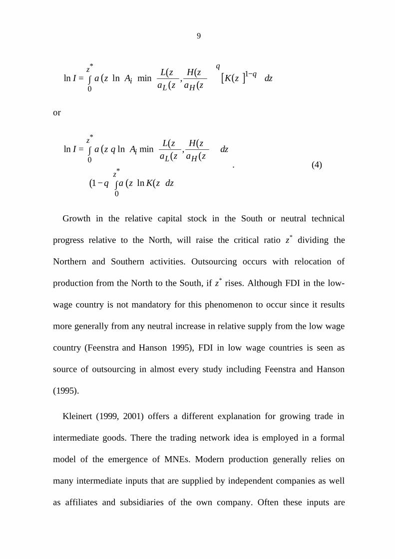
9
( ) ( )( )
( )( )
( )[ ]ln ln min ,*
I z AL z
a zH z
a zK z dzi
L H
z=
∫−α
θθ1
0
or
( ) ( )( )
( )( )
( ) ( ) ( )
ln ln min ,
ln
*
*
I z AL z
a zH z
a zdz
z K z dz
iL H
z
z
=
∫
+ − ∫
α θ
θ α
0
01
. (4)
Growth in the relative capital stock in the South or neutral technical
progress relative to the North, will raise the critical ratio z* dividing the
Northern and Southern activities. Outsourcing occurs with relocation of
production from the North to the South, if z* rises. Although FDI in the low-
wage country is not mandatory for this phenomenon to occur since it results
more generally from any neutral increase in relative supply from the low wage
country (Feenstra and Hanson 1995), FDI in low wage countries is seen as
source of outsourcing in almost every study including Feenstra and Hanson
(1995).
Kleinert (1999, 2001) offers a different explanation for growing trade in
intermediate goods. There the trading network idea is employed in a formal
model of the emergence of MNEs. Modern production generally relies on
many intermediate inputs that are supplied by independent companies as well
as affiliates and subsidiaries of the own company. Often these inputs are
10
specific to the company’s product or production process. When a company
internationalizes its production, the production in the foreign affiliate depends,
at least partly, on the supply of the intermediate inputs from the home country
network of the MNEs. The establishment of a supplier network in the host
country is time-consuming, and many adjustments of the production process
are necessary. Hence, it is cheaper for the foreign affiliate to import
intermediate inputs from the home country. The volume of imported inputs
increases, therefore, in number and size of affiliates of foreign MNEs that
produce in the country. For simplicity, the two country model in Kleinert
(1999) assumes only specific intermediate goods, which must be imported.
Non specific inputs are assumed away. Hence, a foreign affiliate of a MNE
imports all intermediate inputs, a plant in its home country or a national
company imports no inputs. The imports of inputs of the foreign country F,
IF, equal the product of the number of F-based affiliates of MNEs from the
home country H, mH,F, and the value of intermediate inputs used in the
production of an affiliate.
I m pz qzF H F HM
HM= , (5)
pzHM stands for the price index of all (imported) inputs used in the foreign
affiliate of the H-based MNEs, qzHM for the quantities of these inputs. The
superscript M indicates that only affiliates of foreign MNEs import
11
intermediate goods. According to the MNE network explanation, not
companies’ outward FDI of a country is decisive for the amount of imported
inputs but inward FDI of foreign country’s MNEs.
No formal model of global sourcing is presented here. The idea behind
global sourcing can be described as follows: decreasing distance costs and
technological progress, which ease changes in production processes (shorter
product cycle, smaller production series), lead to an increase in the use of
foreign inputs relative to domestic inputs.
In the following two parts, the three explanations will be tested in a cross-
section and a time series analysis. The outsourcing and MNE network
explanation can be tested directly, the global sourcing hypothesis only in a
more indirect manner. In the cross-section analysis the size of the intercept
contains some information about the global sourcing hypothesis: a positive
intercept points to the fact that there is global sourcing, a growing positive
intercept to increased propensity to global sourcing. The global sourcing
hypothesis of increased imported inputs use relies on growing intercepts. In
the time series regression in part four the test of significance of the trend
variable could be interpreted as “test“ of the global sourcing hypothesis. If
there is a tendency towards more intense use of imported input (global
sourcing) this should show up in the time trend variable.
12
3. Evidence from Cross-Section Analyses
3.1. The Data
Intermediate inputs can be derived from input-output tables, which
characterize the interrelations among sectors. The tables show how much oil,
chemicals or steel are used in machinery, for instance. The value of inputs
used in every sector is reported. The OECD (1997) published input-output
tables for ten countries for several years between the late 1960s and 1990. The
economy is divided into 35 sectors, of which 24 are goods producing
industries, 22 of those are manufacturing. These input-output tables include an
imported transaction matrix, which reports the imported inputs of every sector
from every other sector. The total use of intermediate inputs and gross
production of every industry can also be derived from this statistic. Although
the most recent input-output matrix is from 1990, the OECD tables provide a
very impressive data set on the use of imported and domestic inputs and gross
production of every sector over a time span of 20 years (except for Italy of
which only 1985 data are available).
It has been impossible to collect data on sectoral disaggregated inward and
outward FDI stocks of the same quality. Again the OECD offers the best data.
The International Direct Investment Yearbook (1993) reports data on FDI for
23 OECD countries, including all ten countries for which input-output data are
available. The quality of the data differs depending on the national raw data
13
the OECD receives. Especially information on FDI stocks is rather rare. The
United States and Germany report a sectoral breakdown of FDI stocks equal to
the OECD input-output tables back to the late 1970s, Australia’s figures date
back to the early 1980s. Japanese statistics collect only FDI flows, which are
aggregated to stock figures. France started to conduct company surveys of
outward and inward FDI stocks only in the late 1980s and early 1990s.
Statistical data on FDI stocks for the United Kingdom are available from the
mid 1980s for agriculture and eight manufacturing sectors. Although Italian
FDI stock data are available, Italy is excluded from the econometric analysis
because of missing input-output data for 1990. Canada, the Netherlands and
Denmark report no FDI stock data or only of a very small number of sectors.
Therefore, they are excluded. The OECD data of the six countries which are
included in this analysis are filled with data from the national statistics on
which the OECD data is based.
3.2. Cross-Section Estimations
The outsourcing hypothesis can be tested by estimating equation (4). The de-
pendent variable on the left hand side is the logarithm of the imported inputs
which are available from the OECD input output table as described above. For
the six OECD countries under consideration (the North), sectoral disag-
gregated imported input data are used for the analysis. In a cross-section
analysis the first term on the right hand side
14
( ) ( ) ( ) ( ) ( ){ }[ ]α θz A L z a z H z a z dzi L Hz ln min ,0∗
∫ , can be seen as a constant
which is likely to vary among different sectors. It is not necessary to calculate
proxies for this integral. It is sufficient to control for the sectoral differences.
The second term is a product of an unknown coefficient (between zero and
one) and the logarithm of the capital stock used in the production of the
imported inputs: ( ) ( ) ( )1 0− ∫∗
θ α z K z dzz ln . This capital stock is employed in
the foreign country (South). The foreign capital stock can neither be calculated
nor proxied by outward FDI of the inputs’ importing countries. But outward
FDI is the appropriate variable to test the role of globalization (except for the
small share of technology transfer which is not bound to FDI) in outsourcing.
Since FDI in other countries is made responsible for the increase in imported
inputs use in domestic production in many developed countries, this should
show up in the data. Outsourcing in this test is bound to outward FDI and is,
therefore, different from Feenstra and Hanson’s definition, but equal to their
reasoning. Sectoral outward FDI stocks of the input importing country are,
therefore, used as explanatory variable. Outward FDI stocks of sector x are the
sum of all outward FDI stocks of x in any sector y (y=1...n) in the foreign
country. FDI can be chosen as freely by companies as the amount of imported
inputs. The outward FDI stock of a sector fits, therefore, the imported input
15
variable, which is also the sum of imports from all sectors. Equation (4)
changes to
ln lnI c FDI Dummy
Dummy uOutward Sector
Country
= + +
+ +
β β
β1 3
4 . (6)
For the outsourcing hypothesis to hold, β1 must be positive (β1>0). Country
Dummies are included to control for national differences among the six
countries which are together called the North. Australia for instance is likely to
import less inputs because of its distance from its trading partners, the United
States because of its economic size.
The test for the MNE networks is also straight forward. In equation (5)
imported inputs equal the product of the number of affiliates of foreign
companies and their use of intermediate goods. The role of MNEs in a sector
of a host country is proxied by the inward FDI stock in this sector. The inward
FDI stock in x is the sum of all FDI from all foreign sectors y (y=1...n) in
sector x. It fits,therefore, the imported inputs. The use of these data implies
equal intermediate input shares and equal capital coefficients over all sectors.
Sector Dummies shall control for differences among the various sectors.
Taking logs and including a constant, which allows intermediate inputs’
imports by host country companies, the equation to be estimated is given in
(7).
16
ln lnI c FDI Dummy
Dummy uInward Sector
Country
= + +
+ +
β β
β2 3
4(7)
The MNE network hypothesis implies β2>0. The Country Dummies are
included for the same reason as in equation (6). A third equation is estimated
which includes outward and inward FDI stocks.
ln ln lnI c FDI FDI
Dummy Dummy uOutward Inward
Sector Country
= + +
+ + +
β β
β β1 2
3 4(8)
Equation (6), (7) and (8) are tested using sectoral data for three time points:
the late seventies/early eighties, the mid eighties and 1990. The late
seventies/early eighties are tested with data from only three countries:
Germany (1978 data), Japan (1980) and the United States (1982). France and
the United Kingdom did not report FDI stocks at this time, for Australia no
input-output table is available for the early eighties. The number of
observations is rather low: 44, including very few Japanese data. The other
analyses are conducted using data from all six countries. The mid eighties data
are from 1984 for the United Kingdom, from 1985 for France, Japan and the
United States, and from 1986 for Australia and Germany. French stock data
are calculated by using the late eighties stock data and subtract the flow data,
which are reported in OECD (1993).
Figure 1 allows a first glimpse at the data. Imported inputs seem to be
positively related to outward FDI as well as inward FDI for all three time
17
points. Although this is a first indicator, a econometric analysis, which
controls for national and sectoral differences, is needed to make sure that the
correlation does not only depend on sectoral size effects.
Table 1 reports the estimation results for the late seventies/early eighties1.
All regressions are run by using the White (1980) correction for
heteroskedasticity. Columns I to III give the estimates without any dummy
variable, in IV to VI dummies are included to allow for sectoral differences.
1 All estimations are conducted by using the software package EViews 3.1.
18
Figure 1: Imported Inputs and FDI (Mill. $)
1
10
100
1 000
10 000
100 000
1 10 100 1 000 10 000 100 000
Imported Inputs
Outward FDI
1980
1
10
100
1 000
10 000
100 000
1 10 100 1 000 10 000 100 000
Inward FDI
Imported Inputs 1980
1
10
100
1 000
10 000
100 000
1 10 100 1 000 10 000 100 000
Outward FDI
Imported Inputs 1985
1
10
100
1 000
10 000
100 000
1 10 100 1 000 10 000 100 000
Inward FDI
Imported Inputs 1985
1
10
100
1 000
10 000
100 000
1 10 100 1 000 10 000 100 000
Outward FDI
Imported Inputs 1990
1
10
100
1 000
10 000
100 000
1 10 100 1 000 10 000 100 000
Inward FDI
Imported Inputs 1990
19
Table 1: Outsourcing and MNE Networks in the Late Seventies/EarlyEightiesa
Jarque-Bera Prob 0.22 0.65 0.71 0.15 0.48 0.65 0.47 0.16 0.28a Dependent variable: ln(imported inputs); method: least squares; number of observations: 75; Whiteheteroskedasticity-consistent standard errors & covariance. — *, **, *** significant on 10%, 5% and1% level.
F-statistic and R2 are higher in all regressions run with mid eighties data.
The coefficient of the FDIInward variable is of higher significance. As in the
regressions reported in Table 1, significant sectoral differences were found.
2 The R2 and F-statistics presented here are not comparable to the early eighties regression,because the regressions of Table 2 include the Australia Dummy.
23
Dummy variables and production output in regression IV through IX control
for these sectoral differences. Furthermore, the country dummy for Australia
proved to be significant. Australian companies import significantly less input
from other countries than the other economies in this sample which can be
explained by Australia’s geographic location.
The last cross section regressions are presented for 1990, the last year for
which OECD input-output table data are available (Table 3). The sample
includes the same six countries as the mid eighties regression. The lack of
Japanese FDI stock data for petroleum and rubber products and non-metallic
products reduces the number of observations to 73.
a Phillips and Perron (1988). The test is carried out with two lags included, which ensuresfreedom of autocorrelation.— *, **, *** denotes rejection of the hypothesis of an unit root at10%, 5% and 1% level.
In general, the linear combination of two or more integrated variables is
also integrated. However, two variables that are I(1) may be related in an
economically meaningful way, so that the linear combination of the variables
is I(0)3. If variables are related in such a way, it is called cointegration.
Cointegration ensures the absence of a spurious regression problem.
Variables that are I(1) can show a relationship, which stems from the statistical
interrelation of the trends of the I(1) variables, although there exists no long
run economic relationship between these variables (spurious regressions).
Therefore, both pairs of variables, inward FDI and imported inputs and
outward FDI and imported inputs are tested for a cointegration relation using
3 That could stem from the fact that the source of their non-stationarity is the same or thatone of the variables is the source of the non-stationarity of the other variable.
31
the Johansen cointegration test (Johansen 1991). This procedure assumes all
variables to be endogenous and tests for linearly independent cointegration
relations. With only two variables there can be none or one cointegration
relationship. Since the critical values of the test statistics depend on its
specification a choice has to be made among the alternatives for whether a
constant and/or a trend should be included in the specification of the
cointegration equations. Table 5 gives the results of the Johansen cointegration
test for two specifications: (i) constant, no trend in the long run relationship,
and (ii) constant and trend in the long run relationship.
The Johansen cointegration test suggests that there is a stable long run
relationship between the imported inputs and the inward FDI stock but none
between the imported inputs and the outward FDI stock. The LR test, which
uses the Trace statistic, only rejected the hypothesis of no cointegration
equation between inward FDI and imported inputs but could not reject the
hypothesis of one cointegration equation.
32
Table 5: The Johansen Cointegration Testa
Cointegration Rank Trace Statistic 5 Percent Critical Value
Model (i)ln(I) ln(FDIInward)
r=0r=1
22.60165.89298
19.969.24
Model (ii)ln(I) ln(FDIInward)
r=0r=1
33.480211.4447
25.3212.25
Model (i)ln(I) ln(FDIOutward)
r=0r=1
16.44173.98145
19.969.24
Model (ii)ln(I) ln(FDIOutward)
r=0r=1
17.24755.65691
25.3212.25
a lag length: 2
In the next step an error correction model (ECM) is set up to infer an
estimate of the long run relationship of imported inputs and the inward FDI
stock. Furthermore the ECM provides another test for cointegration of the
variables. Given the low number of observations another cointegration test can
yield some information about the robustness of the results obtained.
Therefore, equation (4) and (5) are transformed into a ECM. That gives the
outsourcing hypothesis a second chance.
( ) ( )[ ]∆ ln( ) ( ) ln ln ,I I c FDI Trend
dynamics dummy u
t t Inward t
t
= − − +
+ + +
− −λ β1 1 1 (9)
( ) ( )[ ]∆ ln( ) ( ) ln ln ,I I c FDI Trend
dynamics dummy u
t t Outward t
t
= − − +
+ + +
− −λ β1 1 1 (10)
33
From an economic point of view the error correction term is of special
interest since it gives the long run relationship. Short run dynamics and
dummies are only included to produce well behaved error terms ut. If the
imported inputs deviate from their long run equilibrium, this error will be
corrected in the future. For stability this implies a negative loading coefficient
λ. A high t-value of the loading coefficient points to cointegration. Banerjee et
al. (1998) computed the critical values for the loading coefficient which
indicate a cointegration relation. Table 6 presents the results of the estimation
of equation (9) and (10). The long run relation included a Trend variable
which was dropped because of its insignificance. The short run dynamics are
chosen to ensure normally distributed residuals. The lagged differences (t-1
and t-2) of the endogenous and the exogenous variable were included next to
the unlagged difference of the exogenous variable and a dummy variable
which controls for the sharp decrease in imported inputs in the 1993 recession
in Germany. The insignificant variables were dropped after conducting an
omitted variables test. Since the numbers of observations is very low the
dynamics are kept to a minimum. Tests for autocorrelation up to forth order,
heteroscedasticity, structural breaks, and the Jarque-Bera test were carried out
to ensure that the residuals are well behaved. Interestingly the trend variable
proved to be not significant. This could be seen as the rejection of global
sourcing as an explanation for increasing intermediate products’ imports.
34
Table 6: Outsourcing and MNE Networks in Germany in a Time SeriesAnalysis
ECM (9) ECM (10) Bewley (9)
λa -0.2993** -0.2735
c 2.6419 2.4931 8.8264***
ln(FDIInward, t-1) 0.0975
ln(FDIOutward, t-1) 0.0857
β1 0.3257***
∆ln(It-2) -0.3102*** -0.3479** -1.0364*
∆ln(FDIInward) 0.8249*** 2.7561**
∆ln(FDIOutward, t-2) -0.2026
R 93 -0.18*** -0.2171*** -0.6013**
Adjusted R2 0.84 0.66 0.80
F-Statistic 20.566 8.454 18.523a Banerjee t-statistic. — *, **, *** significant on 10%, 5% and 1% level.
Like the Johansen cointegration test the ECM points to a stable long run
relationship between imported inputs and the inward FDI stock4 but not
between imported inputs and outward FDI. The loading coefficient λ in ECM
(10) is not significantly different from zero, λ in ECM (9) is significant at the
5% level. The long run influence of inward FDI on imported inputs is given
by β1 (=ln(FDIInward, t-1/λ)). Coefficient and significance of the exogenous
variable in the error correction term can easier be seen in the Bewley
transformation of the ECM, which is given in the third column. The Bewley
4 The estimated coefficients of model (i) using the Johansen procedureln(I)=8.921+0.232*ln(FDIInward) (0.71) (0.164) standard deviations in parenthesisare not statistically different from the long run ECM coefficients (without dummy R93) atthe 10% level.
35
transformation is a reformulation of the ECM in order to infer the long run
coefficients directly. The coefficient of β1 equals ln(FDIInward, t-1)/λ. The t value
of this coefficient can be calculated, too. The influence of inward FDI is
positive and significant at the 1% level. A 10% increase of inward FDI
increases imported inputs by 3% according to this estimation. The long run
coefficients and standard deviations are the same in the Bewley transformation
and ECM, the short run differs. Furthermore, a test of weakly exogeniety was
carried out. The hypothesis that inward FDI is weakly exogenous for imported
inputs could not be rejected at the 1% level.
Certainly, the FDI stock is not the only determinant of intermediate input
imports. Imports react strongly to changes in aggregated demand and prices.
Industrial production would be the right exogenous variable to explain the
demand for imported inputs. For this analysis data for value added in German
manufacturing were used, which were taken from the national accounts
(OECD 2000). A change in statistical aggregation methods made it impossible
to use the series for nominal output of manufacturing. To test the influence of
the inward FDI stock if a demand variable is included equation (9) was
changed to equation (11). VA stands for the value added in the manufacturing
sector. The estimated long run coefficients are presented in Table 7.
36
( ) ( ) ( )[ ]∆ ln( ) ( ) ln ln ln ,I I c VA FDI
dynamics dummy u
t t Inw t
t
= − − +
+ + +
− −λ β β1 1 2 1 (11)
Table 7: Estimated Long Run Coefficients
ECM (11) Bewley (11)
λa -0.5352***
c -0.36339 -0.23
ln(Demand t-1) 0.4088
ln(FDIInward, t-1) 0.0885
β1 0.7639**
β2 0.1654
Adjusted R2 0.94 0.97
F-Statistic 35.355 82.896a Banerjee t-statistic. — *, **, *** significant on 10%, 5% and 1% level.
The short run dynamics are chosen to ensure normally distributed residuals.
The cointegration relationship is stable, given the significant loading
coefficient. The size of the coefficient of inward FDI decreased, but remains
positive. The insignificance in the regression based on (11) might stem from
the inefficient estimation procedure. The Johansen cointegration test points to
two cointegration equations among imported inputs, a demand variable and
the inward FDI stock (Table A in the Appendix). The single equation
approach (ECM) is not efficient, a system should be estimated (Harris 1995).
Unfortunately, given the small number of observations it is not possible to
estimate the Johansen procedure.
37
It is interesting to note, that the long run coefficient of inward FDI in the
time series analysis which used German data is quite in line with the results
from the cross section estimations of part three. The coefficient is significant
positive and approximately 0.3, if FDIInward is the only explanatory variable. As
in the cross-section estimation it drops somewhat if a demand variable is
included. Therefore, the MNE network hypothesis could not be rejected
neither in the cross-section nor in the time series analysis.
5. Conclusion
Possible links between trade and FDI have been examined in this paper,
focusing on the influence of FDI on intermediate inputs trade. Cross-sectional
data from six OECD countries and German time series data were employed.
Two possible reasons for the growth in intermediate goods imports were
tested. The outsourcing hypothesis predicts a positive relationship of outward
FDI and imported inputs, the MNE network hypothesis predicts a positive
effect of the level of the inward FDI stock on imported inputs. Global
sourcing remains as an explanation if the other two hypothesis are rejected by
the data.
The MNE network hypothesis could not be rejected by the data, neither in
the cross-sectoral estimations nor in the time series analysis. There is a positive
influence of the inward FDI stock on imported inputs. Foreign affiliates tend
to import significantly more intermediates than domestic companies. There are
38
sectoral and national differences, which show up in the cross section
estimation. It would, therefore, be very interesting to run time series regression
with sectoral disagregated data, which are unfortunately not available.
Furthermore, national differences should be examined by repeating the time
series analysis for other countries. This will be left to further research. The
results of Barrell and te Velde (1999) point to significant differences among
European countries.
There is much less evidence of outsourcing in the data. The German time
series data rejects a long run cointegration relationship between the outward
FDI stock and imported inputs. The cross sectoral regressions did not always
find a significant influence of outward FDI. The effect of outward FDI on
imported inputs is less robust to specification changes. The importance of
outsourcing is believed to differ strongly among sectors. A sectorally
disaggregated time series analysis could, therefore, be especially fruitful for a
test of the outsourcing hypothesis.
Global sourcing is found in the data. There is a large share of imported
inputs, which can not be explained by FDI stocks. However, global sourcing is
rejected as explanation of increased use of imported inputs by the cross-
section and the time series analysis. Certainly, there is global sourcing as well
as outsourcing but these may not be as important as the growing and
39
deepening MNE network to explain the increase in imported inputs used in
production. Global sourcing mainly takes place within MNE networks.
40
Reference List
Andersson, T., and T. Fredriksson (2000). Distinction between intermediateand finished products in intra-firm trade. International Journal ofIndustrial Organization 18: 773–792.
Banerjee, A., J.J. Dolado, and R. Mestre (1998). Error-Correction MechanismTests for Cointegration in a Single Equation Framework. Journal ofTime Series Analysis 19 (3): 267–283.
Barrell, R., and D.W. te Velde (1999). Manufactures Import Demand:Structural Differences in the European Union. 146. National Institute ofEconomic and Social Research, London.
Blomström, M., A. Kokko, and M. Zejan (2000). Foreign Direct Investment:Firm and Host Country Strategies. London, New York: MacmillanPress LTD.
Campa, J., and L.S. Goldberg (1997). Evolving External Orientation ofManufacturing Industries: Evidence from Four Countries. NBERWorking Paper 5919. National Bureau of Economic Research,Cambridge, Mass.
Deutsche Bundesbank (1999). 50 Jahre Deutsche Mark. Frankfurt am Main.
— (various issues). Balance of Payments Statistics. Frankfurt/Main.
Diehl, M. (1999). The Impact of International Outsourcing on the SkillStructure of Employment: Empirical Evidence from GermanManufacturing Industries. Kiel Working Papers 946. The Kiel Instituteof World Economics, Kiel.
Dunlevy, J.A., and W.K. Hutchinson (1999). The Impact of Immigration onAmerican Import Trade in the Late Nineteeth and Early TwentiethCenturies. The Journal of Economic History 59 (4): 1043–1062.
Feenstra, R.C. (1998). Integration of Trade and Disintegration of Production inthe Global Economy. The Journal of Economic Perspectives 12 (4): 31–50.
41
Feenstra, R.C., and G.H. Hanson (1995). Foreign Investment, Outsourcing andRelative Wages. NBER Working Papers 5121. National Bureau ofEconomic Research, Cambridge, Mass.
— (1996). Globalization, Outsourcing and Wage Inequality. AmericanEconomic Review 86 (2 Papers and Proceedings): 240–245.
Gould, D.M. (1994). Immigrant Links and the Home Country: EmpiricalImplications for U.S. Bilateral Trade Flows. Review of Economics andStatistics 76 (2): 302–316.
Harris, R.I.D. (1995). Using Cointegration Analysis in EconometricModelling. London.
Hummels, D.L., D. Rapoport, and K.-M. Yi (1998). Vertical Specialization andthe Changing Nature of World Trade. Economic Policy Review 4 (2):79–99.
Johansen, S. (1991). Estimation and Hypothesis Testing of CointegrationVectors in Gaussian Vector Autoregressive Models. Econometrica 59:1551–1580.
— (1995). Likelyhood-based Inference in Cointegrated Vector AutoregressiveModels. Oxford: Oxford University Press.
Kleinert, J. (1999). Temporal Clusters in Foreign Direct Investment. KielWorking Papers 930. The Kiel Institute of World Economics, Kiel.
— (2001 forthcoming). The Time Pattern of the Internationalisation ofProduction. German Economic Review 2 (1).
Krugman, P.R. (1995). Growing World Trade: Causes and Consequences.Brookings Papers on Economic Activity 1: 327–377.
— (2000). Technology, Trade and Factor Prices. Journal of InternationalEconomics 50 (1): 51–71.
Leamer, E.E. (2000). What's the Use of Factor Content. Journal ofInternational Economics 50 (1): 17–49.
OECD (1993). International Direct Investment Statistics Yearbook. Paris.
— (1997). The OECD Input-Output Database. Paris.
42
OECD (2000). National Accounts II. CD-ROM. Paris.
Phillips, P.C.B., and P. Perron (1988). Testing for a Unit Root in Time SeriesRegression. Biometrika 75: 335–346.
Rauch, J.E. (1999). Networks versus Markets in International Trade. Journalof International Economics 48 (1): 7–35.
White, H. (1980). A Heteroskedasticity-Consistent Covariance Matrix and aDirect Test for Heteroskedasticity. Econometrica 50 (1): 1–26.
43
Appendix
The asymptotic distribution of the LR test statistic for the Johansen
cointegration test depends on assumptions made with the respect to
deterministic trends. Johansen (1995) provides tests for five possibilities. As in
Table 5 results for two are presented in Table A: (i) constant, no trend in the
cointegration equation and, (ii) constant and trend in the cointegration
equation.
Table A: Johansen cointegration test
Cointegration Rank Trace Statistic 5 Percent Critical Value
Model (i)ln(I) ln(VA)ln(FDIInward)
r=0r=1r=2
43.797823.6451 8.9298
34.9119.969.24
Model (ii)ln(I) ln(VA)ln(FDIInward)
r=0r=1r=2
34.4315.8137 1.7823
29.6815.413.76
a lag length: 2
The hypothesis of two cointegration equations could not be rejected for