# Oxford University Press 2005 Oxford Economic Papers 57 (2005), 262–282 262 All rights reserved doi:10.1093/oep/gpi012 Growth, cycles, and stabilization policy By Keith Blackburn* and Alessandra Pelloniy *Centre for Growth and Business Cycle Research, School of Economic Studies, University of Manchester, Manchester M13 9PL; e-mail: [email protected]yDepartment of Economics, University of Rome II, Italy This paper presents an analysis of the joint determination of growth and business cycles with the view to studying the long-run implications of short-term monetary stabiliza- tion policy. The analysis is based on a simple stochastic growth model in which both real and nominal shocks have permanent effects on output due to nominal rigidities (wage contracts) and an endogenous technology (learning-by-doing). It is shown that there is a negative correlation between the mean and variance of output growth irrespective of the source of fluctuations. It is also shown that, in spite of this, there may exist a conflict between short-term stabilization and long-term growth depending on the type of disturbance. Finally, it is shown that, from a welfare perspective, the optimal monetary policy is that policy which maximizes long-run growth to the exclusion of stabilization considerations. JEL classification: E32, E52, O42 1. Introduction A long-standing tradition in macroeconomics—at both theoretical and empirical levels—is the separation of the study of growth from the study of business cycles. The basis of this dichotomy is the presumption that aggregate time series can be decomposed into long-term trends and short-term fluctuations which are deter- mined independently of each other. This presumption runs counter to the implica- tions of endogenous growth theory, according to which any type of shock—be it temporary or permanent, real or nominal—can have a permanent effect on output so long as it changes the amount of resources on which productivity improvements depend (e.g., Stadler, 1990; Pelloni, 1997; Fatas, 2000). Under such circumstances, there is no a priori reason to distinguish between low-frequency and high- frequency variations in economic activity, and the presence of stochastic trends is to be explained not by some arbitrary, exogenous impulse process (e.g., non- stationary productivity shocks), but rather by endogenous responses of technology to changes in the current state of the economy. Recently, the question of precisely how cyclical fluctuations (booms and recessions) might affect secular trends (long-run growth) has been the subject
Transcript
# Oxford University Press 2005 Oxford Economic Papers 57 (2005), 262–282 262All rights reserved doi:10.1093/oep/gpi012
Growth, cycles, and stabilization policy
By Keith Blackburn* and Alessandra Pelloniy
*Centre for Growth and Business Cycle Research, School of Economic Studies,
yDepartment of Economics, University of Rome II, Italy
This paper presents an analysis of the joint determination of growth and business cycles
with the view to studying the long-run implications of short-term monetary stabiliza-
tion policy. The analysis is based on a simple stochastic growth model in which both
real and nominal shocks have permanent effects on output due to nominal rigidities
(wage contracts) and an endogenous technology (learning-by-doing). It is shown
that there is a negative correlation between the mean and variance of output growth
irrespective of the source of fluctuations. It is also shown that, in spite of this, there
may exist a conflict between short-term stabilization and long-term growth depending
on the type of disturbance. Finally, it is shown that, from a welfare perspective,
the optimal monetary policy is that policy which maximizes long-run growth to the
exclusion of stabilization considerations.
JEL classification: E32, E52, O42
1. IntroductionA long-standing tradition in macroeconomics—at both theoretical and empirical
levels—is the separation of the study of growth from the study of business cycles.
The basis of this dichotomy is the presumption that aggregate time series can be
decomposed into long-term trends and short-term fluctuations which are deter-
mined independently of each other. This presumption runs counter to the implica-
tions of endogenous growth theory, according to which any type of shock—be it
temporary or permanent, real or nominal—can have a permanent effect on output
so long as it changes the amount of resources on which productivity improvements
depend (e.g., Stadler, 1990; Pelloni, 1997; Fatas, 2000). Under such circumstances,
there is no a priori reason to distinguish between low-frequency and high-
frequency variations in economic activity, and the presence of stochastic trends
is to be explained not by some arbitrary, exogenous impulse process (e.g., non-
stationary productivity shocks), but rather by endogenous responses of technology
to changes in the current state of the economy.
Recently, the question of precisely how cyclical fluctuations (booms and
recessions) might affect secular trends (long-run growth) has been the subject
of an expanding body of literature. Broadly speaking, one may distinguish
between two contrasting approaches with the potential to generate different
conclusions based on alternative assumptions about the mechanism responsible
for engendering endogenous technological change.1 According to one class of
models—models based on re-allocation effects, whereby the mechanism entails
deliberate actions (purposeful learning) which substitute for production
activities—recessions are events which have a positive impact on growth by
reducing the opportunity cost of diverting resources away from manufacturing
towards productivity improvements (e.g., Aghion and Saint-Paul, 1998a, 1998b).
According to another class of models—models based on externality effects,
whereby the mechanism reflects non-deliberate actions (serendipitous learning)
which are complements to production activity—recessions are episodes which
have a negative influence on growth by lowering factor employment through
which expertise, knowledge and skills are acquired and disseminated (e.g., Martin
and Rogers, 1997, 2000). Within the context of each of these frameworks,
attention has also been given to the question of how growth may be affected
by the precise structure of business cycles in terms of their amplitude,
frequency and persistence. Of particular interest has been the relationship
between growth and volatility with different analyses reaching different conclu-
sions (a positive or negative relationship) depending on what type of model is
employed, what values for parameters are assumed and what types of distur-
bance are considered (e.g., Canton, 1996; Smith, 1996; Martin and Rogers,
1997, 2000; de Hek, 1999; Jones et al., 1999; Aghion and Saint-Paul, 1998a,
1998b; Blackburn and Galindev, 2003; Blackburn and Pelloni, 2004).2
Significantly, all of the above analyses are based on purely real models of the
economy and there are very few investigations that explore the role of monetary
factors. An exception is the recent contribution by Dotsey and Sarte (2000) who
develop a stochastic monetary growth model in which agents are subject to a cash-
in-advance constraint, while operating a simple AK production technology with
a fixed amount of labour. It is shown that an increase in the volatility of monetary
growth, coupled with an increase in average monetary growth, may lead to either
an increase or a decrease in average output growth due to offsetting effects through
k. blackburn and a. pelloni 263
..........................................................................................................................................................................1 In addition to the references that follow, see Ramey and Ramey (1991) and Caballero and Hammour
(1994) for related contributions.2 This conflict in results at the theoretical level is matched by a similar conflict in evidence at the
empirical level. In both cross-section and time series studies, the correlation between the average
growth rate of output and the variability of output growth is found sometimes to be positive (e.g.,
Kormendi and Meguire, 1985; Grier and Tullock, 1989; Caporale and McKiernan, 1996), sometimes to
be negative (e.g., Ramey and Ramey, 1995; Martin and Rogers, 2000; Kneller and Young, 2001),
and sometimes to be zero (e.g., Dawson and Stephenson, 1997; Speight, 1999; Grier and Perry, 2000).
In addition there is evidence to suggest that the correlation is sensitive to the level of disaggregation.
For example, Imbs (2002) reports estimates of a significantly negative correlation when using aggregate
data across countries, but a significantly positive correlation when using disaggregated data across
sectors.
precautionary savings and inflation taxes.3 One objective of the present paper is
to conduct a similar analysis but within the context of a quite different monetary
growth model that allows for endogenous labour, multiple shocks, learning-by-
doing, and nominal rigidities. The last of these features, encapsulated in the form
of one-period wage contracts, does not appear in any of the above literature. Our
analysis provides a further illustration of the joint determination of growth and
business cycles.
A second concern of the paper relates to an important, but largely neglected,
issue in the formulation and evaluation of macroeconomic policy. This is the
extent to which policies designed to stabilize short-run fluctuations might also
affect the long-run performance of the economy. The existence of a relation-
ship between growth and volatility has an obvious bearing on this issue:
depending on whether this relationship is negative or positive, there is the
presumption that successful stabilization would also entail either an improve-
ment or deterioration in growth prospects. The potential significance of this
is self-evident, especially given the fact that it takes only small changes in the
growth rate to produce substantial cumulative gains or losses in output. As
yet, however, there are very few analyses that deal with the issue explicitly.
Two recent contributions that do so are those of Blackburn (1999) and Martin
and Rogers (1997). The former presents a model of imperfect competition
with nominal rigidities in which monetary stabilization policy has a negative
effect on long-run growth. The latter consider a real model of the economy
with perfect competition in which fiscal stabilization policy has a positive effect
on long-run growth. In both cases sustainable growth occurs due to learning-
by-doing which provides the only source of intrinsic dynamics, there being no
capital accumulation or any other propagation mechanism under the direct
control of agents. The models are also highly stylized in a number of other
respects. In Blackburn (1999) there is no explicit optimization by either agents
or policy makers so that the normative aspects of policy are eschewed. In
Martin and Rogers (1997) agents solve only a purely static optimization
problem from which employment is determined as a zero-one variable due to
linear preferences. The analysis that follows is based on a more fully-specified
dynamic general equilibrium model in which both capital accumulation
and wage determination reflect the optimal decision rules of intertemporally
maximizing agents, and in which both the growth and welfare effects of
monetary stabilization policy may be evaluated explicitly.
There are three sources of stochastic fluctuations in our model—a preference
shock, a technology shock, and a monetary growth shock. The central bank
operates a feedback rule for determining how monetary policy responds to each
of these shocks. The first main result of our analysis is that, ceteris paribus,
264 growth, cycles, and stabilization policy
..........................................................................................................................................................................3 The assumption of a positive correlation between the mean and variance of monetary growth
(or inflation) is justified by appealing to empirical evidence.
an increase in the variance of each shock causes both an increase in the variance
and a decrease in the mean of output growth. The latter effect occurs because
of the increase in uncertainty about the state of the economy, in general, and
the response of monetary policy, in particular. Workers react to this greater
uncertainty by setting a higher contract wage at the cost of lower average
employment. This leads to a lower average rate of capital accumulation and,
with it, a lower average growth rate of output. In this way, the model predicts
a negative correlation between short-run (cyclical) volatility and long-run
(secular) growth. Our second main result is that, depending on the type of
shock, a policy that reduces volatility may either increase or decrease growth.
This difference is observed when considering, for example, monetary growth
and technology shocks. In the case of the former, output may be stabilized by
an appropriate (offsetting) response of monetary policy which mitigates varia-
tions in the money supply; this has the effect of reducing nominal uncertainty
which, for reasons just given, leads to higher average employment and higher
average growth. In the case of the latter, output may also be stabilized by
an appropriate policy response, but this now injects fluctuations into the money
supply; as such, nominal uncertainty rises, causing average employment and
growth to fall. A corollary of these findings is that the optimal policy which
minimizes volatility may not only differ from, but may also conflict with, the
optimal policy which maximizes growth. Finally, our third main result is that
the growth-maximizing policy is also the policy that maximizes welfare. This
accords with the view that the welfare effects of business fluctuations are trivial
compared to the welfare effects of growth.
Section 2 contains a description of the model. Section 3 presents the solution
of the model. Section 4 turns to the analysis of growth, volatility and stabilization
policy. Section 5 concludes.
2. The modelWe consider an artificial economy in which there are constant populations
(normalized to one) of identical, immortal households and identical, competitive
firms. The basic structure of this economy is described by a standard stochastic,
monetary growth model. Naturally, whilst the model is more general than some
others, it is constructed in such a way as to focus and simplify the analysis, and is
not meant to provide a complete account of the mechanisms underlying aggregate
fluctuations. In particular, since our intention is to illustrate without having to
resort to numerical simulations, we adopt the usual specifications of preferences
and technologies that admit closed-form solutions.4 The exogenous shocks in the
model are also chosen to provide clear and simple examples of how different
k. blackburn and a. pelloni 265
..........................................................................................................................................................................4 That is, we assume logarithmic utility functions, Cobb-Douglas production functions and 100% rates
of depreciation (e.g., Benassy, 1995; Gali, 1999).
conclusions may be reached on the basis of different assumptions about the sources
of stochastic fluctuations.
2.1 Firms
The representative firm combines Nt units of labour with Kt units of capital to
produce Yt units of output according to
Yt ¼ �t ZtNtð Þ�K1��
t ð1Þ
�t ¼ � expð tÞ ð2Þ
� > 0; � 2 ð0; 1Þ
The term t represents a technology shock which is assumed to be identically,
independently and normally distributed with mean zero and variance �2 . The
term Zt denotes an index of knowledge which is freely available to all firms and
which is acquired through serendipitous learning-by-doing. This provides the
mechanism of endogenous growth in the model. Following convention, we approx-
imate the stock of disembodied knowledge by the aggregate stock of capital which
is taken as given by each firm so that learning takes the form of a pure externality.
Labour and capital are hired from households at the real wage rate Wt/Pt and real
rental rate Rt, respectively, where Wt is the nominal wage and Pt is the price of
output. Profit maximization implies
Wt
Pt¼ ��tZ
�t N
��1t K1��
t ð3Þ
Rt ¼ 1 � �ð Þ�tZ�t N
�t K
��t ð4Þ
2.2 Households
The representative household derives lifetime utility, U, according to
U ¼X1t¼0
�t � logðCtÞ þ� logMt
Pt
� ���tN
�t
� �ð5Þ
�t ¼ � expð�tÞ ð6Þ
� 2 ð0; 1Þ; �;�;� > 0; � > 1;
where Ct denotes consumption and Mt denotes nominal money balances.
To generate a demand function for money, we adopt the familiar short-cut
266 growth, cycles, and stabilization policy
device of introducing money directly into the utility function, rather than
specifying explicitly a separate transactions technology.5 The specification of the
labour term is another feature that our model shares with several others and
encompasses the linear case (�¼ 1) associated either with the assumption of
constant marginal utility of leisure, or with a reduced-form preference ordering
under circumstances where labour is indivisible and individuals choose
employment lotteries in the manner of Hansen (1985) and Rogerson (1988).
The quantity �t represents a preference (or taste) shock, being an identically
and independently distributed normal random variable with mean zero and
variance �2�.6
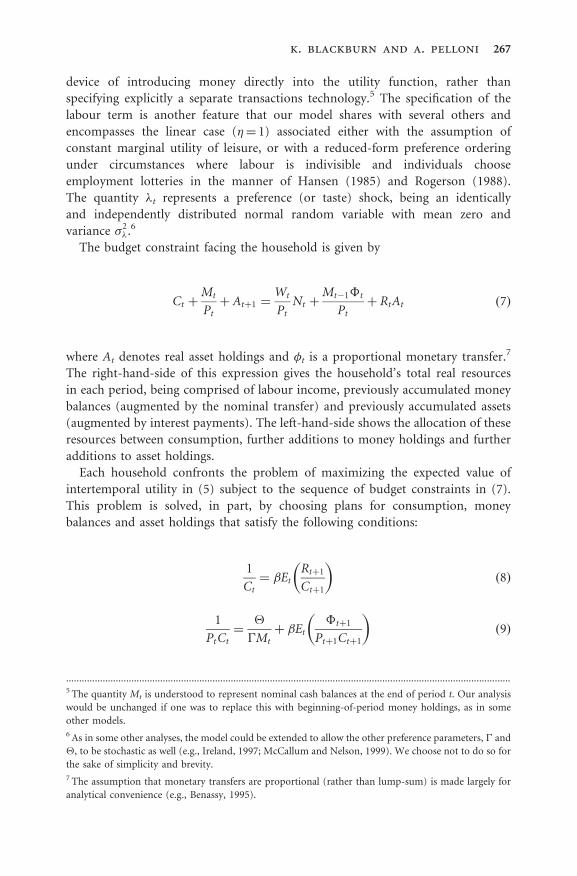
The budget constraint facing the household is given by
Ct þMt
Ptþ Atþ1 ¼
Wt
PtNt þ
Mt�1�t
Ptþ RtAt ð7Þ
where At denotes real asset holdings and �t is a proportional monetary transfer.7
The right-hand-side of this expression gives the household’s total real resources
in each period, being comprised of labour income, previously accumulated money
balances (augmented by the nominal transfer) and previously accumulated assets
(augmented by interest payments). The left-hand-side shows the allocation of these
resources between consumption, further additions to money holdings and further
additions to asset holdings.
Each household confronts the problem of maximizing the expected value of
intertemporal utility in (5) subject to the sequence of budget constraints in (7).
This problem is solved, in part, by choosing plans for consumption, money
balances and asset holdings that satisfy the following conditions:
1
Ct¼ �Et
Rtþ1
Ctþ1
� �ð8Þ
1
PtCt¼
�
�Mtþ �Et
�tþ1
Ptþ1Ctþ1
� �ð9Þ
k. blackburn and a. pelloni 267
..........................................................................................................................................................................5 The quantity Mt is understood to represent nominal cash balances at the end of period t. Our analysis
would be unchanged if one was to replace this with beginning-of-period money holdings, as in some
other models.6 As in some other analyses, the model could be extended to allow the other preference parameters, � and
�, to be stochastic as well (e.g., Ireland, 1997; McCallum and Nelson, 1999). We choose not to do so for
the sake of simplicity and brevity.7 The assumption that monetary transfers are proportional (rather than lump-sum) is made largely for
analytical convenience (e.g., Benassy, 1995).
where Et denotes the expectations operator.8 Each of these conditions has
the usual interpretation of equating the current marginal costs and (expected)
future marginal benefits of foregoing a unit of consumption in favour of an
additional unit of savings (either assets or money). Plans for the number of
hours to work are governed by circumstances in the labour market which we
treat as being imperfectly competitive and imperfectly flexible. We adopt a
standard monopoly union model of wage determination, whereby households
(or unions) set nominal wages and firms determine the level of employment.
We also make the assumption, familiar in business cycle analysis but less so in
growth theory, that wage setting takes place prior to the realizations of shocks
on the basis of one-period contracts. Accordingly, the economy displays
nominal rigidities, as in the early contracting models of Gray (1976) and
Fischer (1977), as well as those of a more recent vintage (e.g., Benassy,
1995; Cho and Cooley, 1995). In contrast to these models, however, we
suppose that the contract wage is chosen so as to maximize households’
expected utility (e.g., Hairault and Portier, 1993; Rankin, 1998), rather than
to satisfy some ad hoc criterion, such as the maximization of other union
objectives or the requirement that the labour market is expected to clear.
When making this choice, workers take account of the response of labour
demand, as expressed in (3). Given this, the optimal wage set at the end of
period t� 1 for period t is found to satisfy9
�Et�1 �tN�t
� �¼ ��WtEt�1
Nt
PtCt
� �ð10Þ
The maximizing behaviour of the representative household is now character-
ized fully by the first-order conditions in (8), (9), and (10), the budget constraint
in (7) and the transversality conditions lim�!1 ��Et Mtþ�=Ptþ�Ctþ�
� �¼
lim�!1 ��Et Atþ�þ1=Ctþ�
� �¼ 0:
2.3 Monetary policy
We assume that monetary policy is governed by a feedback rule through which the
central bank exercises imperfect control over the aggregate money supply. This
feedback rule dictates how the central bank responds to the occurence of exogenous
shocks in the economy. The imprecision in monetary control reflects the assump-
tion that the central bank’s policy instrument is the growth rate of the monetary
268 growth, cycles, and stabilization policy
..........................................................................................................................................................................8 Multiplying these expressions through by � produces the term �/Ct which is understood to be the
marginal utility of consumption, or shadow value of wealth, being equal to the Lagrange multiplier
attached to (7).9 That is, Wt is chosen so as to maximize the expected value of (5) subject to (7) and the condition that
Nt ¼ ðWt=Pt��tZ�t K
1��t Þ
1=ð��1Þ from (3).
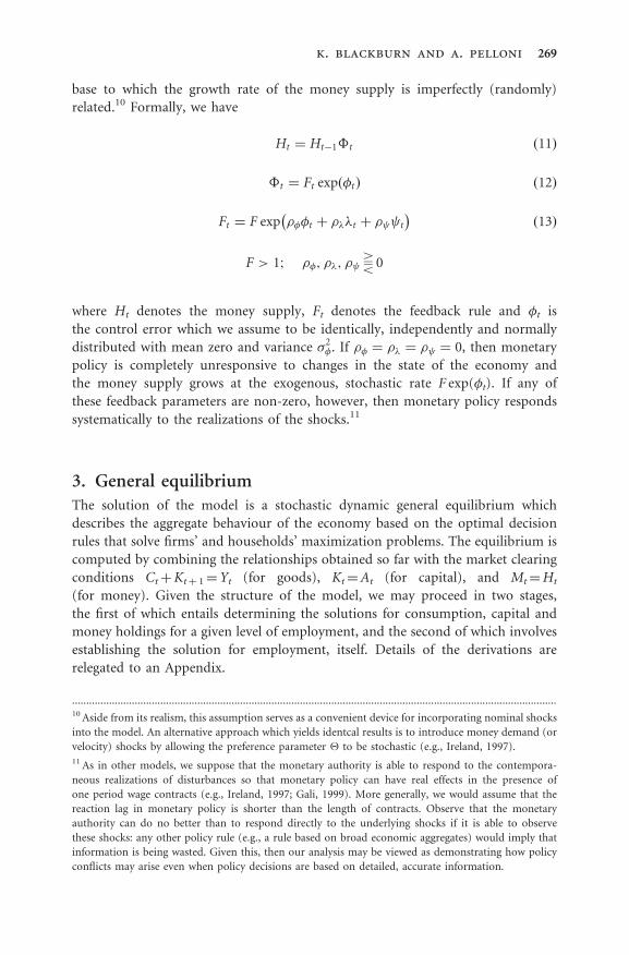
base to which the growth rate of the money supply is imperfectly (randomly)
related.10 Formally, we have
Ht ¼ Ht�1�t ð11Þ
�t ¼ Ft exp �tð Þ ð12Þ
Ft ¼ F exp ���t þ ���t þ � t
� �ð13Þ
F > 1; ��; ��; � T 0
where Ht denotes the money supply, Ft denotes the feedback rule and �t is
the control error which we assume to be identically, independently and normally
distributed with mean zero and variance �2�. If �� ¼ �� ¼ � ¼ 0, then monetary
policy is completely unresponsive to changes in the state of the economy and
the money supply grows at the exogenous, stochastic rate F exp(�t). If any of
these feedback parameters are non-zero, however, then monetary policy responds
systematically to the realizations of the shocks.11
3. General equilibriumThe solution of the model is a stochastic dynamic general equilibrium which
describes the aggregate behaviour of the economy based on the optimal decision
rules that solve firms’ and households’ maximization problems. The equilibrium is
computed by combining the relationships obtained so far with the market clearing
conditions CtþKtþ 1¼Yt (for goods), Kt¼At (for capital), and Mt¼Ht
(for money). Given the structure of the model, we may proceed in two stages,
the first of which entails determining the solutions for consumption, capital and
money holdings for a given level of employment, and the second of which involves
establishing the solution for employment, itself. Details of the derivations are
relegated to an Appendix.
k. blackburn and a. pelloni 269
..........................................................................................................................................................................10 Aside from its realism, this assumption serves as a convenient device for incorporating nominal shocks
into the model. An alternative approach which yields identcal results is to introduce money demand (or
velocity) shocks by allowing the preference parameter � to be stochastic (e.g., Ireland, 1997).11 As in other models, we suppose that the monetary authority is able to respond to the contempora-
neous realizations of disturbances so that monetary policy can have real effects in the presence of
one period wage contracts (e.g., Ireland, 1997; Gali, 1999). More generally, we would assume that the
reaction lag in monetary policy is shorter than the length of contracts. Observe that the monetary
authority can do no better than to respond directly to the underlying shocks if it is able to observe
these shocks: any other policy rule (e.g., a rule based on broad economic aggregates) would imply that
information is being wasted. Given this, then our analysis may be viewed as demonstrating how policy
conflicts may arise even when policy decisions are based on detailed, accurate information.
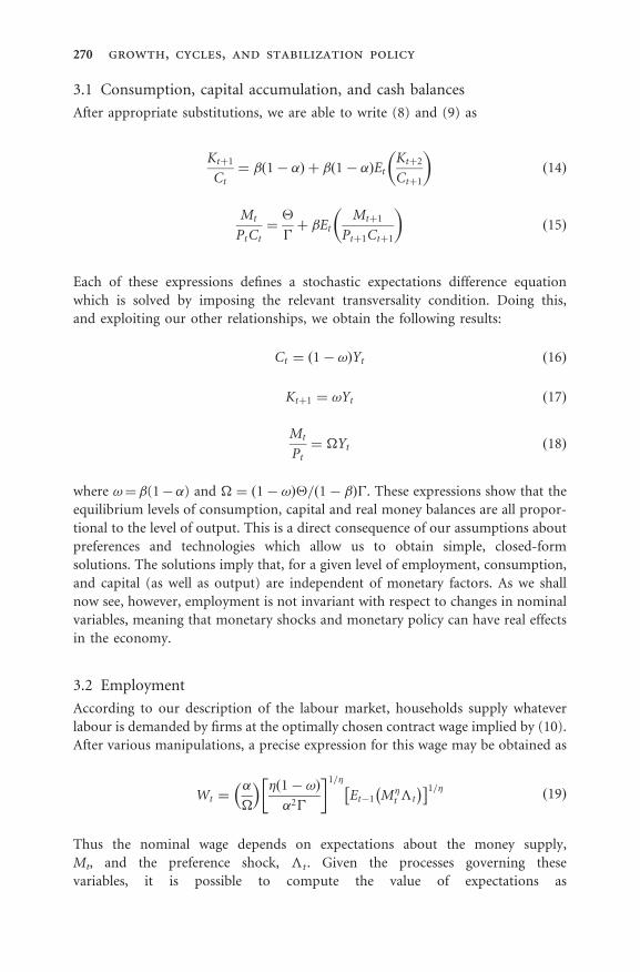
3.1 Consumption, capital accumulation, and cash balances
After appropriate substitutions, we are able to write (8) and (9) as
Ktþ1
Ct¼ � 1 � �ð Þ þ � 1 � �ð ÞEt
Ktþ2
Ctþ1
� �ð14Þ
Mt
PtCt¼
�
�þ �Et
Mtþ1
Ptþ1Ctþ1
� �ð15Þ
Each of these expressions defines a stochastic expectations difference equation
which is solved by imposing the relevant transversality condition. Doing this,
and exploiting our other relationships, we obtain the following results:
Ct ¼ 1 � !ð ÞYt ð16Þ
Ktþ1 ¼ !Yt ð17Þ
Mt
Pt¼ �Yt ð18Þ
where !¼ �(1� �) and � ¼ 1 � !ð Þ�= 1 � �ð Þ�. These expressions show that the
equilibrium levels of consumption, capital and real money balances are all propor-
tional to the level of output. This is a direct consequence of our assumptions about
preferences and technologies which allow us to obtain simple, closed-form
solutions. The solutions imply that, for a given level of employment, consumption,
and capital (as well as output) are independent of monetary factors. As we shall
now see, however, employment is not invariant with respect to changes in nominal
variables, meaning that monetary shocks and monetary policy can have real effects
in the economy.
3.2 Employment
According to our description of the labour market, households supply whatever
labour is demanded by firms at the optimally chosen contract wage implied by (10).
After various manipulations, a precise expression for this wage may be obtained as
Wt ¼�
�
� � � 1 � !ð Þ
�2�
� �1=�
Et�1 M�t �t
� � 1=�ð19Þ
Thus the nominal wage depends on expectations about the money supply,
Mt, and the preference shock, �t . Given the processes governing these
variables, it is possible to compute the value of expectations as
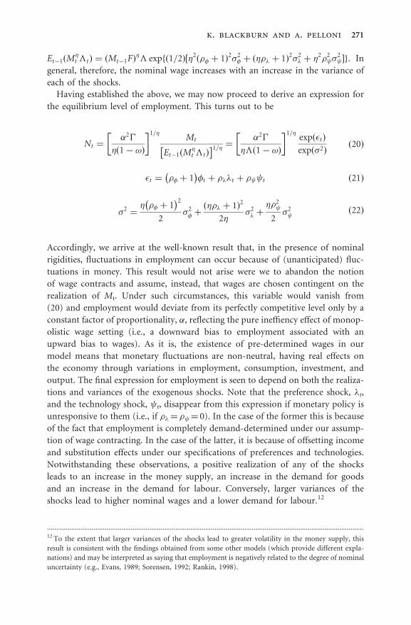
270 growth, cycles, and stabilization policy
Et�1 M�t �tð Þ ¼ Mt�1Fð Þ
�� expfð1=2Þ½�2ð�� þ 1Þ2�2
� þ ��� þ 1ð Þ2�2� þ �
2�2 �
2 �g. In
general, therefore, the nominal wage increases with an increase in the variance of
each of the shocks.
Having established the above, we may now proceed to derive an expression for
the equilibrium level of employment. This turns out to be
Nt ¼�2�
� 1 � !ð Þ
� �1=�Mt
Et�1 M�t �tð Þ
1=�¼
�2�
�� 1 � !ð Þ
� �1=�exp tð Þ
exp �2ð Þð20Þ
t ¼ �� þ 1� �
�t þ ���t þ � t ð21Þ
�2 ¼� �� þ 1� �2
2�2� þ
��� þ 1ð Þ2
2��2� þ
��2
2�2
ð22Þ
Accordingly, we arrive at the well-known result that, in the presence of nominal
rigidities, fluctuations in employment can occur because of (unanticipated) fluc-
tuations in money. This result would not arise were we to abandon the notion
of wage contracts and assume, instead, that wages are chosen contingent on the
realization of Mt. Under such circumstances, this variable would vanish from
(20) and employment would deviate from its perfectly competitive level only by a
constant factor of proportionality, �, reflecting the pure ineffiency effect of monop-
olistic wage setting (i.e., a downward bias to employment associated with an
upward bias to wages). As it is, the existence of pre-determined wages in our
model means that monetary fluctuations are non-neutral, having real effects on
the economy through variations in employment, consumption, investment, and
output. The final expression for employment is seen to depend on both the realiza-
tions and variances of the exogenous shocks. Note that the preference shock, �t,
and the technology shock, t, disappear from this expression if monetary policy is
unresponsive to them (i.e., if ��¼ � ¼ 0). In the case of the former this is because
of the fact that employment is completely demand-determined under our assump-
tion of wage contracting. In the case of the latter, it is because of offsetting income
and substitution effects under our specifications of preferences and technologies.
Notwithstanding these observations, a positive realization of any of the shocks
leads to an increase in the money supply, an increase in the demand for goods
and an increase in the demand for labour. Conversely, larger variances of the
shocks lead to higher nominal wages and a lower demand for labour.12
k. blackburn and a. pelloni 271
..........................................................................................................................................................................12 To the extent that larger variances of the shocks lead to greater volatility in the money supply, this
result is consistent with the findings obtained from some other models (which provide different expla-
nations) and may be interpreted as saying that employment is negatively related to the degree of nominal
4. Stochastic endogenous growth and monetary policyWe are now in a position to address the main issues of interest to us—namely, the
extent to which there are linkages between the cyclical and secular properties of
aggregate fluctuations, and the implications of such linkages for monetary policy.
We do this by solving for the growth rate of output, from which the growth rates of
other non-stationary variables (consumption and capital) may be inferred. These
growth rates are both stochastic and endogenous. It is recalled that we account for
the latter property on the basis of learning-by-doing, formalized by approximating
the stock of disembodied knowledge available to firms by the aggregate stock of
capital: that is, Zt¼Kt in (1). As shown by others, the main implication of this is
to make it possible for the level of output (and, with it, the levels of other variables)
to depend on the accumulated realizations of any type of shock, whether real or
nominal, temporary or permanent. We show this to be true in the present frame-
work. More significantly, we establish the result that the average rate of growth of
output is a function of the variances of the shocks, implying a relationship between
secular growth and cyclical volatility from which we draw further implica-
tions regarding the growth and welfare effects of monetary stabilization policy.
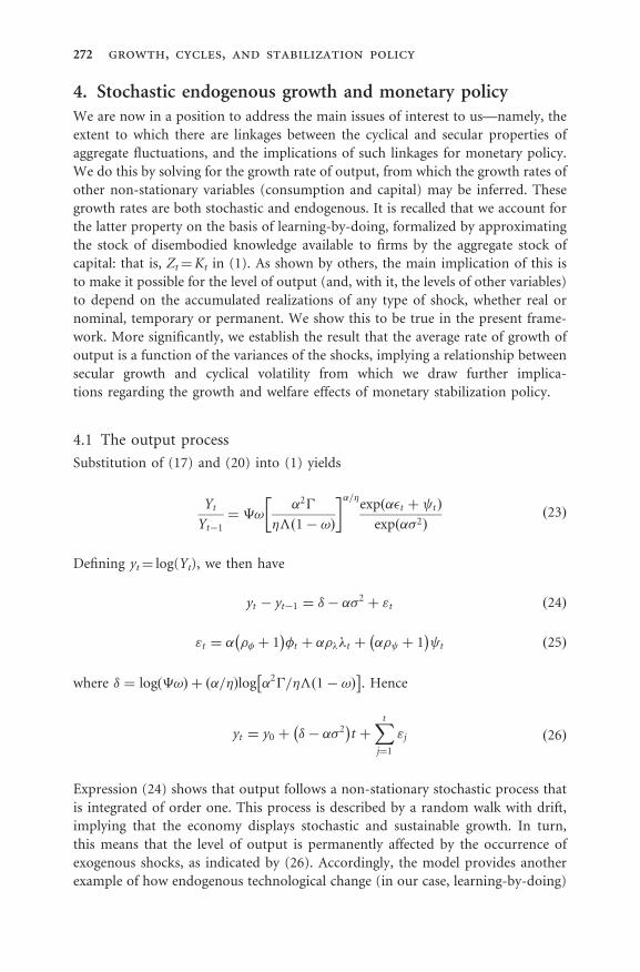
4.1 The output process
Substitution of (17) and (20) into (1) yields
Yt
Yt�1¼ �!
�2�
��ð1 � !Þ
� ��=�exp �t þ tð Þ
exp ��2ð Þð23Þ
Defining yt¼ log(Yt), we then have
yt � yt�1 ¼ � ��2 þ "t ð24Þ
"t ¼ � �� þ 1� �
�t þ ����t þ �� þ 1� �
t ð25Þ
where ¼ log �!ð Þ þ �=�ð Þlog �2�=�� 1 � !ð Þ
. Hence
yt ¼ y0 þ � ��2� �
t þXt
j¼1
"j ð26Þ
Expression (24) shows that output follows a non-stationary stochastic process that
is integrated of order one. This process is described by a random walk with drift,
implying that the economy displays stochastic and sustainable growth. In turn,
this means that the level of output is permanently affected by the occurrence of
exogenous shocks, as indicated by (26). Accordingly, the model provides another
example of how endogenous technological change (in our case, learning-by-doing)
272 growth, cycles, and stabilization policy
can generate unit roots and stochastic trends in macroeconomic time series without
having to assume unit root stochastic processes for exogenous shocks (in particular,
technology shocks).13 Since the growth rate of technology is zt� zt�1¼ yt� yt�1,
we have the standard result of learning-by-doing models that technological change
is pro-cyclical. In addition, since output (like employment) depends positively on
monetary surprises, we have the other standard result of such models that positive
(negative) demand shocks have positive (negative) effects on the growth rate.
Of greater interest to us, however, is the fact that the drift term in (24), � ��2,
depends on the variances of all of the underlying disturbances, as reflected in the
term �2. This is indicative of a relationship between growth and volatility, a matter
to which we now turn.
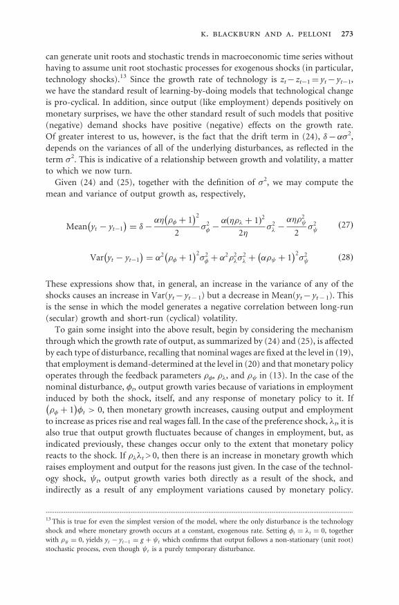
Given (24) and (25), together with the definition of �2, we may compute the
mean and variance of output growth as, respectively,
Mean yt � yt�1
� �¼ �
�� �� þ 1� �2
2�2� �
� ��� þ 1ð Þ2
2��2� �
���2
2�2
ð27Þ
Var yt � yt�1
� �¼ �2 �� þ 1
� �2�2� þ �
2�2��
2� þ �� þ 1
� �2�2 ð28Þ
These expressions show that, in general, an increase in the variance of any of the
shocks causes an increase in Var(yt� yt� 1) but a decrease in Mean(yt� yt� 1). This
is the sense in which the model generates a negative correlation between long-run
(secular) growth and short-run (cyclical) volatility.
To gain some insight into the above result, begin by considering the mechanism
through which the growth rate of output, as summarized by (24) and (25), is affected
by each type of disturbance, recalling that nominal wages are fixed at the level in (19),
that employment is demand-determined at the level in (20) and that monetary policy
operates through the feedback parameters ��, ��, and � in (13). In the case of the
nominal disturbance, �t, output growth varies because of variations in employment
induced by both the shock, itself, and any response of monetary policy to it. If
�� þ 1� �
�t > 0, then monetary growth increases, causing output and employment
to increase as prices rise and real wages fall. In the case of the preference shock, �t, it is
also true that output growth fluctuates because of changes in employment, but, as
indicated previously, these changes occur only to the extent that monetary policy
reacts to the shock. If ���t > 0, then there is an increase in monetary growth which
raises employment and output for the reasons just given. In the case of the technol-
ogy shock, t, output growth varies both directly as a result of the shock, and
indirectly as a result of any employment variations caused by monetary policy.
k. blackburn and a. pelloni 273
..........................................................................................................................................................................13 This is true for even the simplest version of the model, where the only disturbance is the technology
shock and where monetary growth occurs at a constant, exogenous rate. Setting �t ¼ �t ¼ 0, together
with � ¼ 0, yields yt � yt�1 ¼ g þ t which confirms that output follows a non-stationary (unit root)
stochastic process, even though t is a purely temporary disturbance.
If (�� þ 1) t > 0, then there is an overall increase in output. Naturally, the greater
are the variances of the shocks, the greater will be the extent to which output growth
fluctuates, or the greater will be Var(yt� yt� 1). But this is not all that happens—
for our analysis also implies that there will be a reduction in the average growth
rate, or a reduction in Mean(yt� yt� 1). The mechanism in this case is as follows.
As we have seen, a larger variance of each shock is associated with a higher
average wage in (19) and a lower average level of employment in (20). The latter
produces a lower average level of output and, with it, a lower average rate of capital
accumulation. This general reduction in real economic activity is translated into a
reduction in average growth by virtue of a fall in the rate of technological progress
via the process of learning-by-doing.
A negative correlation between growth and volatility is a prediction of some
other models, though the precise mechanism at work is different from that given
above (e.g., Martin and Rogers, 1997, 2000; de Hek, 1999; Jones et al., 1999; Dotsey
and Sarte, 2000; Barlevy, 2002). Beyond the theoretical level, our analysis finds
support in a number of empirical studies which, collectively, suggest that output
growth is negatively related both to the amount of output variability and the degree
of nominal uncertainty (e.g., Kormendi and Meguire, 1985; Grier and Tullock,
1989; Ramey and Ramey, 1995; Judson and Orphanides, 1996; Grier and Perry,
2000; Martin and Rogers, 2000; Kneller and Young, 2001; Imbs 2002).
4.2 Growth, stabilization and welfare
The existence of a relationship between growth and volatility adds a new dimension
to the design and evaluation of macroeconomic policies aimed at stabilizing
fluctuations. As indicated earlier, however, there are very few analyses that
have so far attended to this issue. In the present framework stabilization policy
is modelled explicitly in (13) as a feedback rule for monetary policy through which
the central bank responds endogenously and systematically to realizations of each
of the disturbances. The precise nature of the response in each case is summarized
by the relevant feedback parameter—��, ��, or � —which may be thought of
as being chosen optimally by the bank according to its particular objectives.
Suppose that the central bank is concerned with both reducing short-term volatil-
ity, as given in (28), and enhancing long-term growth, as expressed in (27). In the
case of the nominal shock, �t, there is no conflict between these objectives: from
the perspective of either minimizing Var(yt� yt� 1) or maximizing Mean(yt� yt� 1),
the optimal policy is the same, being to set ��¼�1. Such a policy eliminates
completely the fluctuations and uncertainty that would otherwise arise from this
disturbance, causing a higher level of real activity (because of lower nominal wages)
and a higher rate of technological progress (via learning-by-doing).14 This is an
274 growth, cycles, and stabilization policy
..........................................................................................................................................................................14 Essentially, the central bank operates a policy which effectively gives it perfect control over the money
supply. As indicated previously, the same policy would be optimal for the case in which the nominal
disturbance is a money demand (rather than money supply) shock.
example of how monetary stabilization policy can be complementary to the promo-
tion of growth. A counter-example is provided by consideration of the preference
shock, �t: in this case it is optimal to set ��¼ 0 for minimizing Var(yt� yt� 1), but
��¼�1/� for maximizing Mean(yt� yt� 1). These results are explained by
our earlier observation that employment depends only on the expectation, and
not the realization, of this shock if monetary policy does not respond to it; but a
negative response is called for if one wants to ensure that expectations remain low
so that, on average, wages remain low and employment, output and output growth
remain high. The opposite situation arises with respect to the technology shock, t:
it is now the case that minimizing Var(yt� yt� 1) entails setting � ¼�1/�, while
on the realization of this shock, fluctuations in output can be stabilized, but
only at the cost of raising expectations about the money supply (through greater
nominal uncertainty) so that, on average, wages remain high and real activity
remains low. Thus the model provides a simple illustration of how different sce-
narios may lead to different conclusions about the extent to which there may exist a
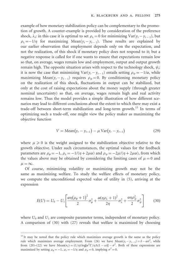
trade-off between short-term stabilization and long-term growth.15 In terms of
optimizing such a trade-off, one might view the policy maker as maximizing the
objective function
V ¼ Mean yt � yt�1
� �� �Var yt � yt�1
� �ð29Þ
where �5 0 is the weight assigned to the stabilization objective relative to the
growth objective. Under such circumstances, the optimal values for the feedback
parameters are ��¼�1, ��¼�1/(�þ 2��) and � ¼�2�/(�þ 2��), from which
the values above may be obtained by considering the limiting cases of �¼ 0 and
�¼1.
Of course, minimizing volatility or maximizing growth may not be the
same as maximizing welfare. To study the welfare effects of monetary policy,
we compute the unconditional expected value of utility in (5), arriving at the
expression
E Uð Þ ¼ U0 � U1
�� �� þ 1� �2
2�2� þ
� ��� þ 1ð Þ2
2��2� þ
���2
2�2
" #ð30Þ
where U0 and U1 are composite parameter terms, independent of monetary policy.
A comparison of (30) with (27) reveals that welfare is maximized by choosing
k. blackburn and a. pelloni 275
..........................................................................................................................................................................15 It may be noted that the policy rule which maximizes average growth is the same as the policy
rule which maximizes average employment. From (24) we have Mean(yt� yt� 1)¼ ���2, while
from (20)–(22) we have Mean ntð Þ ¼ ð1=�Þ log½�2�=�� 1 � !ð Þ� � �2. Both of these expressions are
maximized by setting ��¼�1, ��¼�1/� and � ¼ 0, implying �2¼ 0.
values for the feedback parameters which maximize growth: that is, ��¼�1,
��¼�1/� and � ¼ 0. This implication of our analysis may be viewed within
the context of the broader literature on the welfare costs of economic fluctuations.
The seminal contribution is that of Lucas (1987) whose calculations based on
the neo-classical growth model suggested that the welfare gains from eliminating
business cycles are negligible compared to the welfare gains from maximizing
growth. Significantly, this result has proved to be robust to a number of extensions,
such as changes to the stochastic processes governing shocks (e.g., Obstfeld, 1994),
generalizations of preferences and utility functions (e.g., Obstfeld, 1994;
Pemberton, 1996; Dolmas, 1998; Otrok, 2001) and departures from a world of
complete and perfectly functioning markets (e.g., Imrohoroglu, 1989; Atkeson
and Phelan, 1994; Krusell and Smith, 1999; Beaudry and Pages, 2001;
Storesletten et al., 2001).16 Intuitively, since agents can insure themselves (at least
partially) against fluctuations in income, and since it takes only small changes
in the growth rate to produce substantial cumulative changes in output, then
any benefits that might accrue from lower volatility are eclipsed by the benefits
that arise from higher growth. Given this, then our analysis may be seen as taking
the literature a further step forward by showing explicitly how welfare is maximized
through a policy designed solely to maximize growth, rather than a policy that is
influenced in any way by stabilization objectives. At the same time, our analysis
may also be viewed as providing a qualification to the established wisdom. Since
the growth rate in our model is non-invariant with respect to changes in volatility,
then business fluctuations may well have significant effects on welfare. Some
recent calculations to support this are presented by Barlevy (2002) who obtains
estimates of the costs of fluctuations that far exceed those obtained in previous
studies based on the traditional dichotomy between growth and business cycles.
Naturally, careful interpretation is needed here—for the costs of fluctuations arise
not because of the effects of volatility per se, but rather because of the effects of
volatility on growth. In any event, our analysis lends support to the views that,
from a pure welfare perspective, it is growth, not volatility, that matters the most,
and that it is growth, not volatility, to which macroeconomic policy should be
directed. Indeed, our analysis suggests that policy makers may do rather well
in relinquishing any concern about volatility and focusing, instead, on a simple
growth objective.
5. ConclusionsTwo of the most long-standing traditions in macroeconomics are the study of
growth and the study of business cycles. Until recently, these traditions have
been largely divorced from each other with little cross-fertilization of ideas between
276 growth, cycles, and stabilization policy
..........................................................................................................................................................................16 For these reasons, we believe that our own results concerning welfare would also be robust to various
extensions of the model.
them. With the emergence of endogenous growth theory, however, economists
have began to question the validity of this dichotomy and there is now a growing
body of research that seeks to explore the potential linkages between secular and
cyclical activity. The present paper is intended as a further contribution to this
new and important area of research.
Unlike most other contributions, our analysis allows a role for nominal factors—
nominal shocks and nominal rigidities—in the joint determination of growth
and business cycles. Together with an endogenous technology based on learning-
by-doing, these factors are responsible for generating a stochastic and sustainable
growth rate of output, the mean and variance of which are both dependent on the
variances of both real and nominal shocks. In this way, the model is able to account
for a negative relationship between long-run growth and short-run volatility in
accordance with the findings of several empirical studies.
Another distinguishing feature of our analysis is the attention given to the role
of policy—in particular, stabilization policy. Indeed, it is one of only a very few
investigations that provide fully worked-out examples of how policies designed to
mitigate the impact of exogenous shocks can have consequences for the long-run
performance of the economy. The possibility of this adds a new dimension to the
design and evaluation of such policies, the most important aspect of which may not
be their stabilization qualities per se, but rather their potential to influence long-
term growth prospects. According to our own investigation, monetary stabilization
policy aimed at reducing stochastic fluctuations may work either for or against the
promotion of long-run growth depending on the source of the fluctuations. This
result is notable in itself and is made more notable by the fact that the optimal
policy which maximizes welfare is not the policy which minimizes volatility but the
policy which maximizes growth.
Our analysis is intended to be illustrative, being based deliberately on an
analytically tractable framework for which closed-form solutions can be obtained
from appropriate assumptions about preferences and technologies. The alternative
approach would have been to use a more complicated model under more general
assumptions and to conduct the analysis via numerical simulations. We have no
reason to believe that the basic message of the paper would have been different had
we followed this alternative which could have led one to lose sight of the precise
objectives of the exercise and the intuition underlying the results. Nevertheless,
it would be interesting to acquire an idea of the orders of magnitude of involved,
and we intend to pursue this in later work by conducting a quantitative analysis
of a more general, calibrated version of the model.
Acknowledgements
The authors are grateful for the comments of two anonymous referees on an earlier
version of the paper, and for the financial support of the Leverhulme Trust and the ESRC
(grant no. L138251030). The usual disclaimer applies.
k. blackburn and a. pelloni 277
References
Aghion, P. and Saint-Paul, P. (1998a) On the virtue of bad times: an analysis of theinteraction between economic fluctuations and productivity growth, MacroeconomicDynamics, 2, 322–44.
Aghion, P. and Saint-Paul, P. (1998b) Uncovering some causal relationships betweenproductivity growth and the structure of economic fluctuations: a tentative survey,Labour, 12, 279–303.
Atkeson, A. and Phelan, C. (1994) Reconsidering the costs of business cycles with incom-plete markets, NBER Macroeconomics Annual, 187–207.
Barlevy, G. (2002) The costs of business cycles under endogenous growth, mimeo,Department of Economics, Northwestern University.
Beaudry, P. and Pages, C. (2001) The costs of business cycles and the stabilisation value ofunemployment insurance, European Economic Review, 45, 1545–72.
Benassy, J-P. (1995) Money and wage contracts in an optimising model of the business cycle,Journal of Monetary Economics, 35, 303–15.
Blackburn, K. (1999) Can stabilisation policy reduce long-run growth?, Economic Journal,109, 67–77.
Blackburn, K. and Galindev, R. (2003) Growth, volatility and learning, Economics Letters, 79,417–21.
Blackburn, K. and Pelloni, A. (2004) On the relationship between growth and volatility,Economics Letters, 83, 123–128.
Caballero, R. and Hammour, M. (1994) The cleansing effect of recessions, AmericanEconomic Review, 84, 350–68.
Canton, E. (1996) Business cycles in a two sector model of endogenous growth, mimeo,Centre for Economic Research, University of Tilburg.
Caporale, T. and McKiernan, B. (1996) The relationship between output variabiity andgrowth: evidence from post-war UK data, Scottish Journal of Political Economy, 43, 229–36.
Cho, J.O. and Cooley, T.F. (1995) The business cycle with nominal contracts, EconomicTheory, 6, 13–33.
Dawson, J.W. and Stephenson, E.F. (1997) The link between volatility and growth: evidencefrom the states, Economics Letters, 55, 365–69.
Dolmas, J. (1998) Risk preferences and the welfare cost of business cycles, Review ofEconomic Dynamics, 1, 646–76.
Dotsey, M. and Sarte, P.D. (2000) Inflation, uncertainty and growth in a cash-in-advanceeconomy, Journal of Monetary Economics, 45, 631–55.
de Hek, P.A. (1999) On endogenous growth under uncertainty, International EconomicReview, 40, 727–44.
Evans, G.W. (1989) The conduct of monetary policy and the natural rate of unemployment,Journal of Money, Credit and Banking, 21, 498–507.
Fatas, A. (2000) Endogenous growth and stochastic trends, Journal of Monetary Economics,45, 107–28.
Fischer, S. (1977) Long-term contracts, rational expectations and the optimal money supplyrule, Journal of Political Economy, 85, 163–90.
278 growth, cycles, and stabilization policy
Gali, J. (1999) Technology, employment and the business cycle: do technology shocksexplain aggregate fluctuations?, American Economic Review, 89, 249–71.
Gray, J. (1976) Wage indexation: a maroeconomic approach, Journal of Monetary Economics,2, 221–35.
Grier, K.B. and Perry, M.J. (2000) The effects of real and nominal uncertainty on inflationand output growth: some Garch-M evidence, Journal of Applied Econometrics, 15, 45–58.
Grier, K.B. and Tullock, G. (1989) An empirical analysis of cross-national economic growth,1951–1980, Journal of Monetary Economics, 24, 259–76.
Hairault, J-O. and Portier, F. (1993) Money, new-Keynesian macroeconomics and thebusiness cycle, European Economic Review, 37, 1533–68.
Hansen, G.D. (1985) Indivisible labour and the business cycle, Journal of MonetaryEconomics, 16, 309–28.
Imbs, J. (2002) Why the link between volatility and growth is both positive and negative,Discussion Paper No. 3561, Centre for Economic Policy Research, London.
Imrohoroglu, A. (1989) Cost of business cycles with indivisibilities and liquidity constraints,Journal of Political Economy, 97, 1364–83.
Ireland, P.N. (1997) A small structural quarterly model for monetary policy evaluation,Carnegie-Rochester Conference Series on Public Policy, 47, 83–108.
Jones, L.E., Manuelli, R.E., and Stacchetti, E. (1999) Technology (and policy) shocks inmodels of endogenous growth, Working Paper No. 7063, NBER, Cambridge, MA.
Judson, R. and Orphanides, A. (1996) Inflation, volatility and growth, mimeo, Board ofGoverners of the Federal Reserve System, Washington, DC.
Kneller, R. and Young, G. (2001) Business cycle volatility, uncertainty and long-run growth,Manchester School, 69, 534–52.
Kormendi, R. and Meguire, P. (1985) Macroeconomic determinants of growth: cross-country evidence, Journal of Monetary Economics, 16, 141–63.
Krusell, P. and Smith, A. (1999) On the welfare effects of eliminating business cycles, Reviewof Economic Dynamics, 2, 245–72.
Lucas, R.E. (1987) Models of Business Cycles, Basil Blackwell, Oxford.
Martin, P. and Rogers, C.A. (1997) Stabilisation policy, learning-by-doing, and economicgrowth, Oxford Economic Papers, 49, 152–66.
Martin, P. and Rogers, C.A. (2000) Long-term growth and short-term economic instability,European Economic Review, 44, 359–81.
McCallum, B.T. and Nelson, E. (1999) An optimising IS-LM specification for monetarypolicy and business cycle analysis, Journal of Money, Credit and Banking, 31, 296–316.
Obstfeld, M. (1994) Evaluating risky consumption paths: the role of intertemporal substi-tutability, European Economic Review, 38, 1471–86.
Otrok, C. (2001) On measuring the welfare cost of business cycles, Journal of MonetaryEconomics, 47, 61–92.
Pelloni, A. (1997) Nominal shocks, endogenous growth and the business cycle, EconomicJournal, 107, 467–74.
Pemberton, J. (1996) Growth trends, cyclical fluctuations and welfare with non-expectedutility preferences, Economics Letters, 50, 387–92.
k. blackburn and a. pelloni 279
Ramey, G. and Ramey, V.A. (1991) Technology commitment and the cost of economicfluctuations, Working Paper No. 3755, National Bureau of Economic Research,Cambridge, MA.
Ramey, G. and Ramey, V.A. (1995) Cross-country evidence on the link between volatilityand growth, American Economic Review, 85, 1138–52.
Rankin, N. (1998) Nominal rigidity and monetary uncertainty, European Economic Review,42, 185–99.
Rogerson, R. (1988) Indivisible labour, lotteries and equilibrium, Journal of MonetaryEconomics, 21, 3–16.
Sorensen, J.R. (1992) Uncertainty and monetary policy in a wage bargaining model,Scandinavian Journal of Economics, 94, 443–55.
Speight, A.E.H. (1999) UK output variability and growth: some further evidence, ScottishJournal of Political Economy, 46, 175–81.
Stadler, G.W. (1990) Business cycle models with endogenous technology, AmericanEconomic Review, 80, 150–67.
Storesletten, K., Telmer, C., and Yaron, A. (2001) The welfare cost of business cyclesrevisited: finite lives and cyclical variation in idiosyncratic risk, European EconomicReview, 45, 1311–39.
AppendixThe results in (16), (17), and (18) may be computed as follows. Substitution of (4) into (8)delivers
1
Ct¼ � 1 � �ð ÞEt
Ytþ1
Ctþ1Ktþ1
� �ðA1Þ
which may be transformed into (14) by exploiting Yt¼CtþKtþ1. Repeated substitution in(14) implies
Ktþ1
Ct¼ 1 � �ð Þ
���EtKtþ�þ1
Ctþ�
� �þX�i¼1
1 � �ð Þ�½ �i
ðA2Þ
Imposing the transversality condition lim�!1 ��Et Ktþ�þ1=Ctþ�
� �¼ 0 yields the solution
Ktþ1
Ct¼
� 1 � �ð Þ
1 � � 1 � �ð ÞðA3Þ
Combining (A3) with Yt¼CtþKtþ1 gives the expressions in (16) and (17). Similarly, (11) inconjunction with Ht¼Mt implies that (9) may be converted to (15), for which repeated
280 growth, cycles, and stabilization policy
substitution produces
Mt
PtCt¼ ��Et
Mtþ�
Ptþ�Ctþ�
� �þ
�
�
� �X��1
i¼0
�i ðA4Þ
Imposing the transversality condition lim�!1 ��Et Mtþ�=Ptþ�Ctþ�
� �¼ 0 gives the solution
Mt
PtCt¼
��
1 � �ð Þ�ðA5Þ
Together with (16), (A4) yields the expression in (18).The results in (19) and (20) may be derived in the following manner. Substitution of
(3) and (16) into (10) gives
�Et�1 �tN�t
� �¼
�2T
1 � !ðA6Þ
In turn, (3) and (18) may be combined to obtain
Nt ¼�
�
� � Mt
Wt
� �ðA7Þ
which implies
�Et�1 �tN�t
� �¼ �
�
�
� �� Et�1 M�t �tð Þ
W�t
ðA8Þ
Equating (A8) with (A6) yields the expression in (19). The value of expectations inthis expression is computed by substituting for �t and Mt using (6), (11), (12), and (13)to obtain Et�1 M�
t �tð Þ ¼ Mt�1Fð Þ��Et�1½expð�ð�� þ 1Þ�t þ ð��� þ 1Þ�t þ �� tÞ�, and
exploiting the fact that E½expðxÞ� ¼ expð12 �
2Þ if x is a normally distributed random variable
with mean zero and variance �2. The result in (20) is then derived by combining (19)with (A7) and making similar substitutions to form Mt¼Mt�1F exp(t), where t isdefined in (21), and ½Et�1ðM
�t �t�
1=�¼ Mt�1F�
1=�fEt�1½expð�ð�� þ 1Þ�t þ ð��� þ 1Þ�tþ
�� t�g1=�
¼ Mt�1F�1=� expð�2
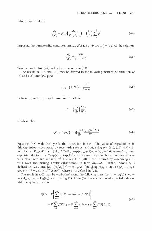
Þ, where �2 is defined in (22).The result in (30) may be established along the following lines. Let ct ¼ log Ctð Þ; mt ¼
logðMt=PtÞ; nt ¼ log Ntð Þ and kt ¼ log Ktð Þ. From (5), the unconditional expected value ofutility may be written as
EðUÞ ¼ EX1t¼0
�t �ct þ�mt ��tN�t
( )
¼ �X1t¼0
�tE ctð Þ þ�X1t¼0
�tE mtð Þ þX1t¼0
�tE �tN�t
� � ðA9Þ
k. blackburn and a. pelloni 281
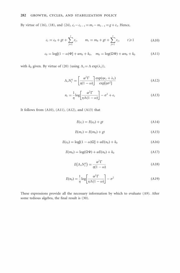
By virtue of (16), (18), and (24), ct� ct� 1 ¼mt�mt� 1¼ gþ "t. Hence,