43
Growth Effects of Sports Franchises, Stadiums, and Arenas: 15 Years Later Dennis Coates September 2015 MERCATUS WORKING PAPER
| Date post: | 30-May-2018 |
| Category: |
Documents |
| Upload: | trinhduong |
| View: | 220 times |
| Download: | 0 times |

Growth Effects of Sports Franchises, Stadiums, and
Arenas: 15 Years Later
Dennis Coates
September 2015
MERCATUS WORKING PAPER
Dennis Coates. “Growth Effects of Sports Franchises, Stadiums, and Arenas: 15 Years Later.” Mercatus Working Paper, Mercatus Center at George Mason University, Arlington, VA, September 2015. Abstract A 1999 study by Dennis Coates and Brad R. Humphreys found the presence of major sports franchises to have no significant impact on the growth rate of per capita personal income and to be negatively correlated with the level of per capita personal income for a sample of all cities that had been home to at least one franchise in any of three professional sports—baseball, basketball, and football—at some time between 1969 and 1994. This paper returns to the questions Coates and Humphreys asked using an additional 17 years of data and a number of new stadiums, arenas, and franchises. The data cover 1969–2011 and add hockey and soccer franchises to the mix while also including all standard metropolitan statistical areas rather than just those that housed franchises in the major professional leagues. The analysis also adds two new dependent variables: wage and salary disbursements and wages per job. The results here are generally similar to those of Coates and Humphreys; the array of sports variables, including presence of franchises, arrival and departure of clubs in a metropolitan area, and stadium and arena construction, is statistically significant. However, individual coefficients frequently indicate harmful effects of sports on per capita income, wage and salary disbursements, and wages per job. JEL codes: Z2, Z28 Keywords: economic impact, sports, sports economics, stadium, arena, sports franchise, sports league, baseball, basketball, football, hockey, soccer Author Affiliation and Contact Information Dennis Coates Professor of Economics Department of Economics, University of Maryland, Baltimore County [email protected] Acknowledgments This paper was supported by research assistance from the Mercatus Center at George Mason University. I thank Brian M. Deignan for his efforts putting together the data for the project. All studies in the Mercatus Working Paper series have followed a rigorous process of academic evaluation, including (except where otherwise noted) at least one double-blind peer review. Working Papers present an author’s provisional findings, which, upon further consideration and revision, are likely to be republished in an academic journal. The opinions expressed in Mercatus Working Papers are the authors’ and do not represent official positions of the Mercatus Center or George Mason University.

3
Growth Effects of Sports Franchises, Stadiums, and Arenas
15 Years Later
Dennis Coates
I. Introduction
A 1999 study by Coates and Humphreys found the presence of major sports franchises to have
no significant impact on the growth rate of per capita personal income and to be negatively
correlated with the level of per capita personal income for a sample comprising all cities that had
been home to at least one franchise in any of three professional sports—baseball, basketball, and
football—at some time between 1969 and 1994. This paper returns to the questions asked by
Coates and Humphreys (1999) using an additional 17 years of data and a number of new
stadiums, arenas, and franchise movements. The data here cover 1969 through 2011 and add
hockey and soccer franchises to the mix. They also include all standard metropolitan statistical
areas (SMSAs) rather than just those areas that housed franchises in the major professional
leagues. The analysis also adds two new dependent variables: wage and salary disbursements and
wages per job. The results here are generally similar to those of Coates and Humphreys (1999);
the array of sports variables, including presence of franchises, arrival and departure of clubs in a
metropolitan area, and stadium and arena construction, is statistically significant. However,
individual coefficients frequently indicate a negative relationship between sports and per capita
income, wage and salary disbursements, and wages per job.
Sports is big business, especially team sports such as football, basketball, and baseball.
Whether the issue is contracts for professional players, contracts for broadcast rights, or
universities switching conferences, the amounts of money involved seem unreal to most people.
Given the money that changes hands in the business of sports, thinking that this business has a

4
large influence on the local economy of the cities or metropolitan areas where the teams play is
natural. Indeed, communities around the country are told frequently of the large economic effects
of building a new stadium or arena and of acquiring or losing a team. Cities, counties, and states
often find a way to subsidize construction of sports facilities and, in recent times, to subsidize
operating expenses, too; they do so partly in response to the promised economic results.
The size and even the existence of these effects have been the subject of a large body of
literature over the past 20 years. Several reviews of the literature exist, and this paper will
discuss the broader literature in more detail in the next section. Coates and Humphreys (1999)
was the first study in this literature to include in a single (time-series cross-section) regression all
the cities that hosted at least one franchise from the National Football League (NFL), National
Basketball Association (NBA), or Major League Baseball (MLB) at any point during the period
1969 to 1996. Moreover, that study’s analysis includes variables for stadium and arena
construction, for entry and exit of franchises, and for stadium and arena capacities, as well as for
the presence of franchises for each of the three sports separately. Coates and Humphreys refer to
this array of variables as the sports environment. They found that the entire sports environment
matters for the level of real personal income per capita, in the sense that the array of sports
variables are jointly statistically significant. But contrary to the promised increase, the presence
of a major sports franchise lowers the income.
Whereas the array of sports variables is jointly statistically significant, few of the
variables are individually so. Joint significance combined with individual insignificance can
occur if individual variables are highly correlated and separating their individual influences is
not possible. One solution to this problem is to obtain more data. As previously stated, this study
returns to the analysis of Coates and Humphreys (1999) but with an additional 17 years of data.

5
In the intervening period, a large number of new stadiums and arenas have been built, more
teams have relocated, and some new teams have come into existence. In addition, the large
number of stadiums built in the early and middle 1990s have now been around well beyond their
“honeymoon” period, thus enabling an examination of their long-term effects that was not
possible in the original Coates and Humphreys paper. Also, this expanded dataset provides the
potential to get more precise estimates of the effects of individual sports and the effects of entry
and exit and to reassess the two questions posed by Coates and Humphreys in 1999: (1) whether
franchises, stadiums, and arenas affect the level of income per capita in a community and (2)
whether they alter the rate of growth of income per capita.
The results of this exercise are largely consistent with the findings of Coates and Humphreys
(1999) and of numerous other studies that have found that the effect of sports franchises and
stadium and arena construction on local economies is weak or nonexistent. Indeed, franchises,
stadiums, and arenas may be harmful rather than beneficial to the local community. Moreover, the
results are not limited to per capita personal income but hold also for wage and salary disbursements
and wages per job, two outcomes not considered by Coates and Humphreys in 1999.
The next section of this paper provides a summary of the existing literature on the effect
of sports franchises on local economies. Subsequent sections describe the data, the estimating
strategy, and the results, respectively. The final section restates the main findings and the
contribution of this paper.
II. Literature
The literature on the effects of stadiums and sports on local economies began in earnest with
papers by Robert Baade and Richard Dye (1988, 1990) and Baade (1996). Baade and Dye (1990)
6
examined data covering 1965 to 1983 for nine cities and found that the effect of a stadium or
franchise on the level of real income in those cities is uncertain. They also found that a stadium
has a negative effect on a city’s share of the region’s income. Using a much larger sample than in
Baade and Dye (1990), Baade (1996) found no effect on income. His focus then turned to the
city’s share of state employment in the amusement and recreation sector and in the commercial
sports industry. Baade’s analysis focuses on 10 cities covering periods from 1964–1989 for
Cincinnati to 1977–1989 for Denver. The results are mixed. For some cities, the number of
stadiums—or the number of teams—is positive and significant. For others, the variables are
negative and significant or not significant. When the cities are pooled into a single sample,
neither the number of teams nor the number of stadiums is statistically significant.
Coates and Humphreys (1999) criticize the methodologies used by Baade and Dye (1990)
and Baade (1996) for two reasons. First, the models suffer from omitted variables bias. The
analyses have too few controls for the circumstances of the local and national economies and, in
the case of Baade (1996), treat all sports and all facilities as if they would have equal effects.
Coates and Humphreys (1999) suggest that it is likely that a football stadium used for games
fewer than 10 times a year would have a different effect than a baseball stadium used 81 times a
year. Hence, they split the sports variables by sport and facility type. Second, the dependent
variable is in many specifications defined as a share variable. An increase in the city’s share of
state or regional employment may mean that overall employment rose—just faster in the city
than elsewhere—or it may mean that the city took jobs from the rest of the state or region. The
latter possibility is good for the city but clearly bad for the rest of the state. However, the former
is not necessarily good for anyone, even the city. Suppose the stadium or franchise effect is to
reduce employment everywhere, but by more outside the city than within it. In such a case, the

7
city’s share of employment will rise, but the stadium or franchise will not benefit either the city
or the state. For those reasons, Coates and Humphreys (1999) eschew share variables in their
analysis, focusing instead on the level and growth rates of real personal income per capita in the
metropolitan areas.
Since Coates and Humphreys (1999), the literature on the effect of franchises and sports
facilities on local communities has expanded rapidly. Although the focus on changes in income
remained (Gius and Johnson 2001; Nelson 2001, 2002; Wassmer 2001; Santo 2005; Rappaport
and Wilkerson 2001; Lertwachara, K. and J. Cochran 2007; Austrian and Rosentraub 2002;
Davis and End 2010), subsequent research also looked for effects (1) on employment and wages
by sectors of the economy (Coates and Humphreys 2003, 2011; Hotchkiss, Moore, and Zobay
2003; Miller 2002); (2) on sales tax collections (Coates 2006; Coates and Depken 2009, 2011;
Baade, Baumann and Matheson 2008); (3) on rents (Carlino and Coulson 2004; Coates and
Gearhart 2008; Coates and Matheson 2011); (4) on property values (Tu 2005; Feng and
Humphreys 2008; Humphreys and Feng 2012); and (5) on hotel occupancy rates (Lavoie and
Rodríguez 2005). Analysis expanded to specific events, including all-star games, championships,
and mega-events such as the Olympics or FIFA (Fédération Internationale de Football
Association) World Cup (Hotchkiss, Moore and Zobay 2003; Madden 2006; Porter 1999; Porter
and Fletcher 2008; Baade and Matheson 2001, 2004a, 2006; Coates and Humphreys 2002;
Coates, 2006, 2012, 2013; Coates and Depken 2011; Matheson 2005; Coates and Matheson
2011; Leeds 2007); strikes and lockouts (Coates and Humphreys 2001; Zipp 1996); auto racing
(Baade and Matheson 2000; Coates and Gearhart 2008); and collegiate events such as bowl
games and the NCAA (National Collegiate Athletic Association) Men’s Basketball Final Four
Championship (Baade and Matheson 2004b; Baade, Baumann, and Matheson 2011; Coates and

8
Depken 2009, 2011). For more details on the literature, see Siegfried and Zimbalist (2000, 2006);
Coates and Humphreys (2008), and Coates (2007).
Few studies have found evidence that sports franchises, stadium or arena construction, or
hosting of events such as the Olympics, World Cup, or Super Bowl generate benefits measurable
in greater incomes, employment, or tax collections across broad metropolitan area economies.
The two most prominent of these studies are Carlino and Coulson (2004) and Hotchkiss, Moore,
and Zobay (2003). Findings from both studies have been questioned, and the studies and their
criticisms are discussed in detail. Carlino and Coulson (2004) use data from the 1993 and 1999
versions of the American Housing Survey to estimate a pseudo-panel model of rents in the 60
largest metropolitan areas. Their models include a dummy variable for the presence of an NFL
team as well as an array of housing, neighborhood, and city characteristics variables. Focusing on
their results for housing units within the central city of the metropolitan areas, they report that the
presence of an NFL franchise induces about an 8 percent increase in monthly rent. Carlino and
Coulson interpret this increase as a measure of the social benefit of the football team. However,
when observations from outside the central city are included, the estimated impact of the franchise
becomes statistically insignificant, with four of five point estimates negative. Coates, Humphreys,
and Zimbalist (2006) criticize Carlino and Coulson’s analysis of the central city observations for a
variety of methodological issues, including the sensitivity of the results to inclusion or exclusion
of some explanatory variables whose presence dramatically alter the sample size.
Hotchkiss, Moore, and Zobay (2003) find that the 1996 Atlanta Olympics had a
beneficial effect on employment and wages. Using a difference-in-differences approach, they
find that counties that hosted events or were near to counties that hosted events saw
employment grow 17 percent faster than counties that neither hosted nor were near to counties
9
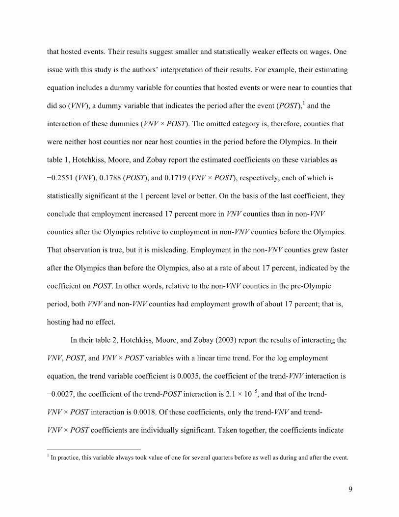
that hosted events. Their results suggest smaller and statistically weaker effects on wages. One
issue with this study is the authors’ interpretation of their results. For example, their estimating
equation includes a dummy variable for counties that hosted events or were near to counties that
did so (VNV), a dummy variable that indicates the period after the event (POST),1 and the
interaction of these dummies (VNV × POST). The omitted category is, therefore, counties that
were neither host counties nor near host counties in the period before the Olympics. In their
table 1, Hotchkiss, Moore, and Zobay report the estimated coefficients on these variables as
−0.2551 (VNV), 0.1788 (POST), and 0.1719 (VNV × POST), respectively, each of which is
statistically significant at the 1 percent level or better. On the basis of the last coefficient, they
conclude that employment increased 17 percent more in VNV counties than in non-VNV
counties after the Olympics relative to employment in non-VNV counties before the Olympics.
That observation is true, but it is misleading. Employment in the non-VNV counties grew faster
after the Olympics than before the Olympics, also at a rate of about 17 percent, indicated by the
coefficient on POST. In other words, relative to the non-VNV counties in the pre-Olympic
period, both VNV and non-VNV counties had employment growth of about 17 percent; that is,
hosting had no effect.
In their table 2, Hotchkiss, Moore, and Zobay (2003) report the results of interacting the
VNV, POST, and VNV × POST variables with a linear time trend. For the log employment
equation, the trend variable coefficient is 0.0035, the coefficient of the trend-VNV interaction is
−0.0027, the coefficient of the trend-POST interaction is 2.1 × 10⁻⁵, and that of the trend-
VNV × POST interaction is 0.0018. Of these coefficients, only the trend-VNV and trend-
VNV × POST coefficients are individually significant. Taken together, the coefficients indicate
1 In practice, this variable always took value of one for several quarters before as well as during and after the event.

10
that employment in host counties and counties near host counties trends downward before and
after the Olympics, although less quickly after the Olympics.
Feddersen and Maennig (2013) also cast doubt on the findings of Hotchkiss, Moore, and
Zobay (2003). First, rather than the quarterly data used by Hotchkiss, Moore, and Zobay,
Feddersen and Maennig analyze monthly employment data. Consequently, their figures can
focus more precisely on the time period of the event and the pre- and post-event periods.
Second, Feddersen and Maennig have data by sector. Hence, the effects of hosting the Olympics
can be traced to those sectors where they are most likely to occur, such as tourism, so that
employment growth in unlikely sectors, such as manufacturing or financial services, is not
attributed to the Olympics. Their conclusions are that (1) there is no persistent evidence of long-
term employment boost attributable to the Olympics and (2) any increases that occurred were
exclusively in Fulton County, the host to most of the events, during the month of the
competition. Feddersen and Maennig’s use of disaggregated data also reveals that the increased
employment is limited to three sectors: arts, entertainment, and recreation; retail trade; and
accommodation and food services.
The upshot is that doubt has been cast on the two most prominent academic pieces
reporting positive general economic benefits: Carlino and Coulson (2004) and Hotchkiss, Moore,
and Zobay (2003). Consequently, Coates, Humphreys, and Zimbalist (2006) and Feddersen and
Maennig (2013) imply there is little evidence of general increases in income, wages and
employment, tax collections, or rents and property values associated with the sports
environment.
What other favorable evidence exists comes bundled with unfavorable evidence, as in the
case of Baade and Dye (1990), described previously. Within a given city, although a broad-based

11
benefit may be absent, localized benefits may exist. For example, property values near a stadium
or arena may increase, as Tu (2005), Feng and Humphreys (2008), and Humphreys and Feng
(2012) find. Each of these studies explicitly addresses the possibility that the effect of a stadium
or arena may vary over the metropolitan area. In each case, property values are the dependent
variable, with distance from a facility the explanatory variable of most interest. Each study finds
that the closer to the facility a property is, the higher its property value will be. As distance from
the facility grows, the boost to property value declines. Coates and Humphreys (2006) and
Ahlfeldt and Maennig (2012) find support for this possibility in referendums on stadium
subsidies that show that the likelihood of a favorable vote is greater in precincts closer to the
facility than in precincts farther away.
Indeed, localized benefits of this sort form the basis for some recommendations for
stadiums and arenas as effective methods of urban revitalization (Austrian and Rosentraub 2002;
Rosentraub 2006; Cantor and Rosentraub 2012; Nelson 2002; Santo 2005). These studies suggest
downtown revitalization is beneficial, even at the cost of losses imposed on citizens living
outside the central city. Indeed, the studies argue that urban renewal in the central city benefits
the entire metropolitan area, though not in ways that are reflected in personal income. Coates
(2007), however, contends that this urban renewal argument is just one of several forms of
justification for income redistribution associated with stadium and arena development projects.
III. Data
The data for this project come from multiple sources. The dependent variables in the analysis are
personal income per capita, wage and salary disbursements, and wages per job, which come from
the US Department of Commerce’s Bureau of Economic Analysis (BEA) website. Coates and

12
Humphreys (1999) focus on personal income per capita and the growth in personal income per
capita, but their subsequent work includes analysis of wages and salaries within specific sectors
of the economy (Coates and Humphreys 2003) and analysis of earnings (Coates and Humphreys
2011). Wage and salary disbursements and wages and salaries per job are included in this
analysis to enable focus on labor income as in these later studies.
The data cover the period 1969–2011 for each of 366 BEA metropolitan statistical areas
(MSAs). These metropolitan areas are cities and all or parts of the economically integrated
surrounding counties. The BEA consistently defines each area over the entire period by going
back and adjusting the original data to be consistent with the modern circumstances. Of the 366
MSAs, 46 were home to a franchise in one or more of the American Basketball Association
(ABA), MLB, Major League Soccer (MLS), NBA, NFL, or National Hockey League (NHL) for
some period during the years from 1969 through 2011. Table 1 (page 29) lists the 46 MSAs that
hosted a franchise; the remaining 320 MSAs are listed in an appendix that is available on the
Internet or by request to the author.
Personal income per capita, wage and salary distribution, and wages per job are deflated
using the national annual average of the CPI-U (consumer price index for all urban consumers),
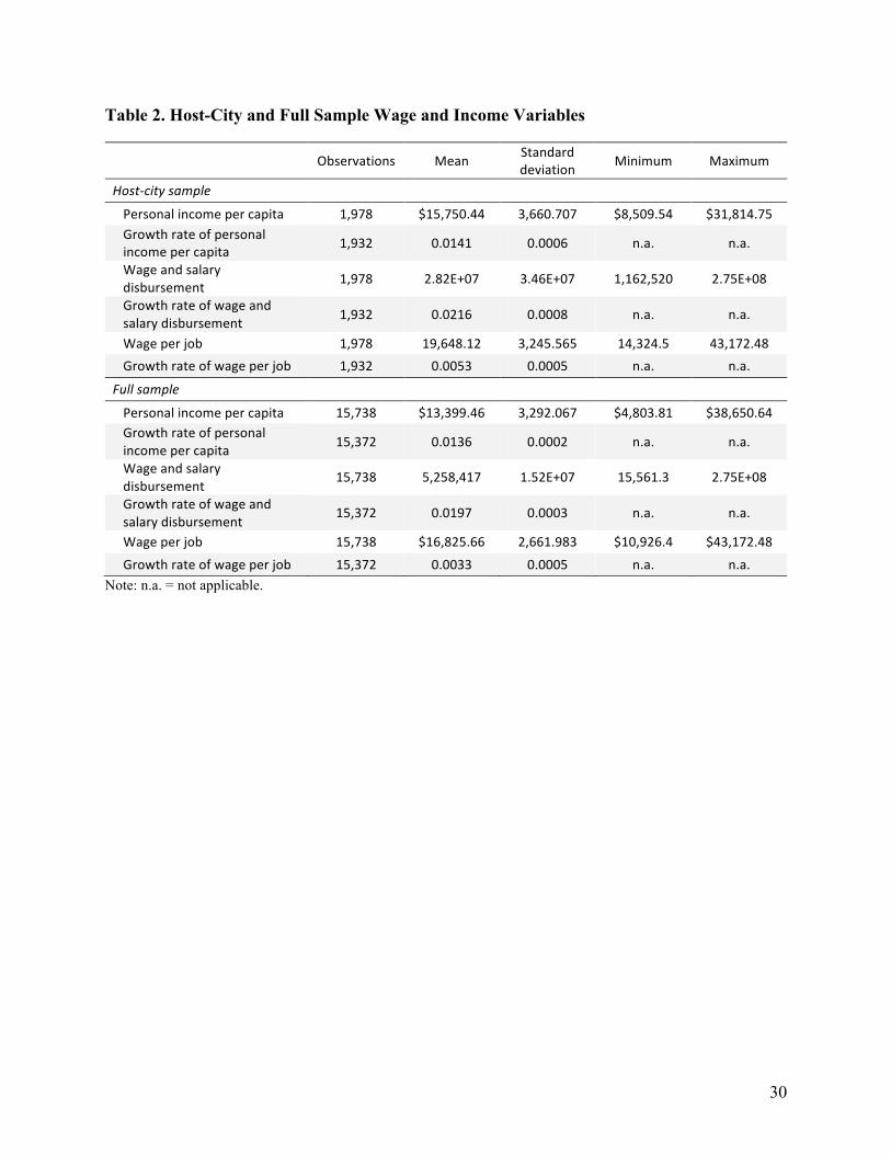
with 1982–1984 equal to 100. Table 2 (page 30) provides descriptive statistics for these income
variables, for both the full sample and the host-city subsample. For the 366 MSAs over the time
period, the average growth rate in real personal income per capita is 1.3 percent. The average
level of real personal income per capita is $13,399 (over 15,738 local area–years, or 43 years for
each of 366 MSAs). Mean growth in real personal income per capita in these 46 areas is 1.41
percent per year; mean real personal income per capita is $15,750. For areas that never had a
franchise, the growth rate of real personal income per capita is 1.36 percent and mean real

13
personal income per capita is $13,062. Average annual population in the areas that had
franchises is 2.75 million; for those that never had a franchise the average annual population is
256,493. Average annual population growth rates are 1.30 percent for the areas that had
franchises and 1.29 percent in areas that did not. Neither the growth rate of real personal income
per capita nor the population growth rates are statistically significantly different between areas
with and without franchises.
The explanatory variables in the models include the lagged value of the dependent
variable, whether that variable is the level, the log, or the growth rate; population growth; an
array of sports environment variables; city and year effects; or city-specific time trends. The
sports environment variables are defined as in Coates and Humphreys (1999) with the addition of
variables indicating NHL franchises, ABA franchises, and before and after hosting the Winter or
Summer Olympics.
Each sport has a variable that indicates if an area hosted a professional team from that
sport during a specific year. For example, in the New York City area, the MLB dummy
variable will have a value of 1 in every year because the area had an MLB team in every year
from 1969 through 2011. However, for the Washington, DC, area, the MLB dummy will be 1
for the years 1969, 1970, and 1971, when the Washington Senators played, and for the years
2005–2011, when the Washington Nationals played. But the MLB dummy will have a value of
0 for 1972–2004, the period when Washington, DC, was without an MLB franchise. Similar
variables identify the years in which the areas had NFL, NBA, NHL, and MLS franchises.
Note that no area had an MLS franchise before 1996, the year the league was founded. The
analysis does not account for the presence of professional soccer clubs before 1996 although
several short-lived leagues existed. Likewise, the analysis makes no accounting of the various

14
short-lived football and hockey leagues, except the teams from those leagues that joined the
NFL or NHL.
The ABA began play in the mid-1960s and competed against the NBA until the two
leagues merged in the mid 1970s. Similarly, the American Football League (AFL) began play in
1960 and merged with the NFL in 1970. The two leagues agreed to a merger in 1966, with the
creation of the Super Bowl being part of that merger agreement. However, the two leagues did
not integrate their schedules until 1970. The analysis includes the ABA as a separate league for
the few years of its existence in the early years of the data, and the cities that hosted teams in
this league are so identified. For the period when the ABA joined the NBA, its existence is
reflected in the NBA variable, and the ABA variable becomes 0. Those cities that did not join
the NBA—Louisville and St. Louis—obviously have a value of 0 for the NBA variable.
Because all the clubs from the AFL merged into the NFL and the agreement to merge came
before 1969, the earliest year of our data, cities hosting AFL clubs in those early years are
identified as having NFL clubs.
During the analysis period, areas acquired teams and lost teams. Areas that lost teams did
so because an existing team moved to another area. Cities obtained teams either by attracting an
existing team away from some other area or by being granted an expansion franchise. Cities and
states have spent a great deal of money playing the stadium game. They have offered—or have
been forced—to build a stadium to keep a team from leaving town or to bring a team to town,
either through expansion or relocation of a franchise. The analysis includes variables that
identify the year a team arrived in an area and the subsequent nine years. Other variables identify
the year a franchise fled a location and the subsequent nine years. Franchises from all five sports
relocated, and all the leagues expanded, so franchise arrival and departure indicators exist for all

15
five sports. Variables for construction of a stadium or arena in each sport are also included.
These too identify the first 10 years a facility is open. Stadium capacity and capacity squared are
included for each sport as an indicator of whether a stadium has multiple uses (that is, houses
both football and baseball teams or only one). Likewise, a variable identifies arenas that house
both an NBA and an NHL franchise. A variable identifies those few team years in which a
basketball club played in a domed stadium.
Finally, four variables identify the pre- and post-Olympic host periods for Los Angeles,
Atlanta, and Salt Lake City. All four variables have a value of 1 in each of the two years before
and after the event and in the year of the event. This overlap is done because identifying prior
and posterior effects of a mid-year event is impossible with only annual data.
IV. Empirical Model
The empirical approach taken in this paper is to estimate a panel data model with and without
clustered standard errors. Clustering is by the MSA and allows the error term for each MSA to
have a unique variance. Clustering has no effect on coefficient estimates, but it does alter the
standard errors of the estimates, thereby leading to potentially different inferences from
hypothesis tests. Formally,
𝑦!" = 𝛼! + 𝛾𝑦!"!! + 𝛽!!! 𝑥!"# + 𝜕!𝑡! + 𝜇! + 𝜀!",
where 𝑦 represents the outcome of interest (either the level, the log, or the growth rate of real
personal income per capita; wage and salary disbursements; or wages per job); 𝑥 represents the
explanatory variables (such as the sports environment variables); 𝑡! indicates an SMSA-specific
time trend; 𝛼, 𝛾, 𝛽, 𝛿, and 𝜇 are parameters to be estimated; and 𝜀 is a random error with a mean
of 0 and variance that may differ by metropolitan area 𝑖.

16
The model is intended to capture as much of the systematic variation in the dependent
variable as possible with the nonsports variables. The lagged dependent variable and the SMSA
fixed effects capture persistence in the dependent variable that may arise from the industrial
structure, political organization and regulatory environment, geography and climate, and other
local factors that either are time invariant or evolve only slowly. The purpose is to capture all
those sources of income or wages and salaries that are inherent in the economic structure of the
locality so that the sports variables do not inadvertently explain outcomes that are rightly
attributed to other factors.
The model includes the lagged value of the dependent variable as well as SMSA fixed
effects and SMSA-specific time trends, as does Coates and Humphreys (1999). Angrist and
Pischke (2008) argue that models that include both fixed effects and lagged dependent variables
require very stringent and unlikely assumptions for consistent estimation. Estimating the model
with either lagged dependent variables or fixed effects imposes less stringent assumptions, but
those models are not equivalent, nor is one model nested within the other. However, Angrist and
Pischke (2008) demonstrate that estimates from the two models bound the true causal effect of
the “treatment.” Specifically, if the true model includes the lagged dependent variable but is
mistakenly estimated with fixed effects, estimates of the causal effect will be larger than the true
effects. Whereas if the true model is fixed effects but is mistakenly estimated with the lagged
dependent variable, then the true effects are larger than the estimated effects. To maintain
comparability with Coates and Humphreys (1999), this study estimates the equation with both
fixed effects and the lagged dependent variable and with each separately to obtain the upper and
lower bounds described by Angrist and Pischke (2008).

17
Consistent with Coates and Humphreys (1999), the null hypothesis is that all of the 𝛽
attached to sports environment variables are 0, indicating that the sports environment has no
effect on the dependent variable. The alternative hypothesis is that at least one of the sports
coefficients is different from 0.
V. Results
It is important to determine whether the various measures of income in the sample are stationary.
If they are not, then coefficient estimates will be biased and inconsistent, and inferences
regarding the influence of sports on the local economy are unreliable. The panel unit root test of
Im, Pesharan, and Shin (2003) is used to test for stationarity of the data. This test allows serial
correlation in the variable being tested to be different for each MSA. In the test, the null
hypothesis is that the data are nonstationary—that is, they have a unit root in each panel. The
alternative hypothesis is that at least one panel is stationary. I test for stationarity on the full
sample of MSAs and on the host-city subsample (that is, those host cities that had a franchise at
some time during the data time period). I also test for stationarity of the natural logarithm and the
annual growth rate of the real value of the dependent variables. Each model includes a trend, and
separate unit root tests are conducted using one, two, and three lags of the dependent variable.
Table 3 (page 31) summarizes the panel unit root tests. In the full sample of 366 MSAs
and the 46 host-city subsample of the MSAs, the level and the log of real personal income per
capita are nonstationary, whereas the annual growth rate (computed as the difference in the log
values from year to year) is stationary. Considering real wage and salary disbursements, the Im,
Pesharan, and Shin (2003) tests reject the null of unit roots for all SMSAs in the full sample and
in the host-city subsample, regardless of whether the variable is in level, logs, or growth rate. For

18
the log of wages per job, the null hypothesis is not rejected in either sample but is rejected for
levels and the growth rate.
Three dependent variables are possible, each of which is estimated in levels, logs, and
growth rates. They are also estimated either with fixed city effects or with the lagged dependent
variable as an explanatory variable, or with both. The models are estimated on the full sample of
cities and the subsample of host cities. In addition, with year fixed effects and city-specific time
trends, as well as the array of sports environment variables, each regression has a great many
coefficient estimates. However, specific coefficients are not of particular interest, so the large
array of estimates is in an appendix available from the author on request or on the Internet. The
focus in this discussion of the results is on the joint significance of groups of sports variables: (1)
the full set, (2) those indicating presence of a franchise, (3) those indicating entry, (4) those
indicating exit, (5) those indicating stadium and arena capacity, (6) those indicating construction
of new facilities, and (7) those indicating Summer or Winter Olympic host. Generally, the groups
of variables are jointly significant, with the exception of the Olympic host group. The estimation
results are also used to compute the sports and nonsports contributions to the dependent
variables. These predictions consistently indicate that the sports contribution is relatively small
and, in some cases, negative.
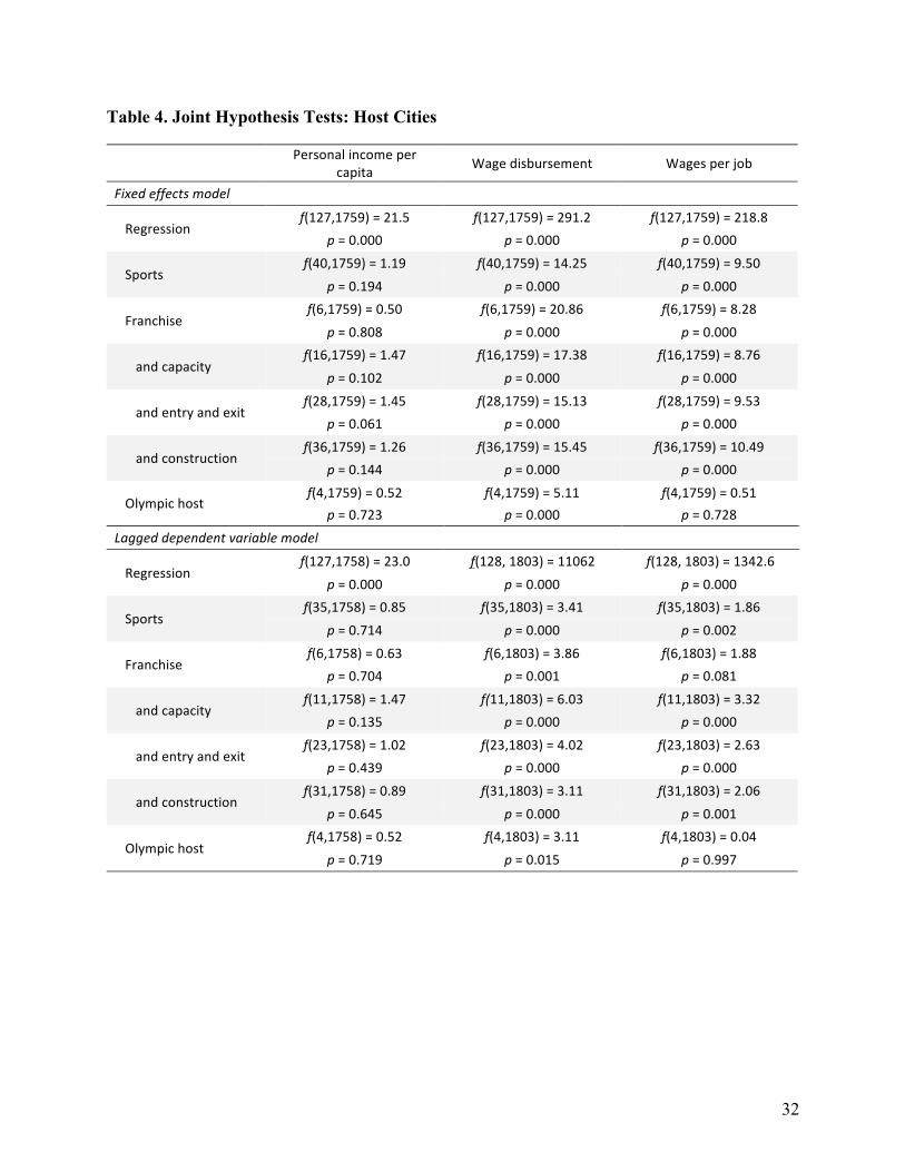
Tables 4 and 5 (pages 32 and 33) report F-statistics and p-values for joint hypothesis
tests. First, the tables report the test of significance of the regression. In each case, the null
hypothesis is easily rejected. More relevant for the purpose of this paper, the tables report the
statistics for the null hypothesis (1) that all sports variables have zero coefficients, (2) that
variables indicating the presence of a franchise have a zero coefficient, (3) that the franchise and
stadium and arena capacity variables all have zero coefficients, (4) that the coefficients in item
19
(3) and all entry and exit variables have zero coefficients, and (5) that all coefficients in item (4)
plus the facility construction variables all have zero coefficients. The tables also report the
results for the null that the pre- and post-Olympic host variables all have zero coefficients. All
test results are reported for both the host-city and full samples and for models using only city
fixed effects or using only lagged values of the dependent variable. Results in tables 6 and 7
(pages 34 and 35) are not based on clustered standard errors.
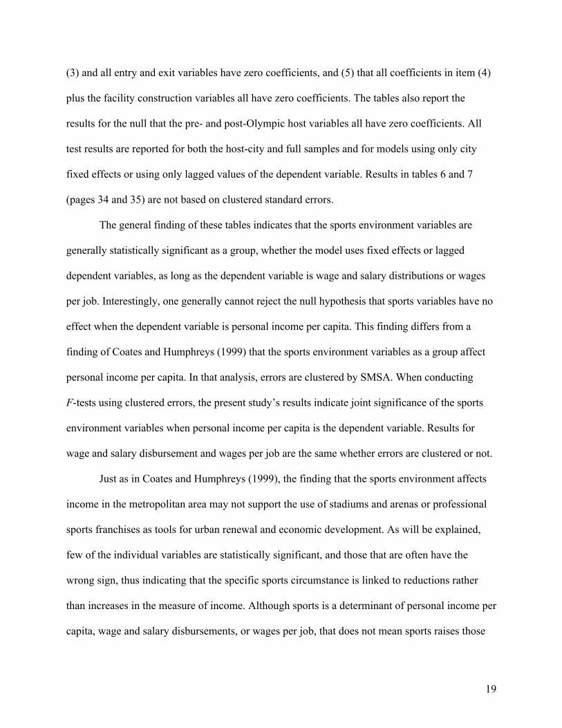
The general finding of these tables indicates that the sports environment variables are
generally statistically significant as a group, whether the model uses fixed effects or lagged
dependent variables, as long as the dependent variable is wage and salary distributions or wages
per job. Interestingly, one generally cannot reject the null hypothesis that sports variables have no
effect when the dependent variable is personal income per capita. This finding differs from a
finding of Coates and Humphreys (1999) that the sports environment variables as a group affect
personal income per capita. In that analysis, errors are clustered by SMSA. When conducting
F-tests using clustered errors, the present study’s results indicate joint significance of the sports
environment variables when personal income per capita is the dependent variable. Results for
wage and salary disbursement and wages per job are the same whether errors are clustered or not.
Just as in Coates and Humphreys (1999), the finding that the sports environment affects
income in the metropolitan area may not support the use of stadiums and arenas or professional
sports franchises as tools for urban renewal and economic development. As will be explained,
few of the individual variables are statistically significant, and those that are often have the
wrong sign, thus indicating that the specific sports circumstance is linked to reductions rather
than increases in the measure of income. Although sports is a determinant of personal income per
capita, wage and salary disbursements, or wages per job, that does not mean sports raises those
20
variables; joint significance does not mean that the sports environment is beneficial for the local
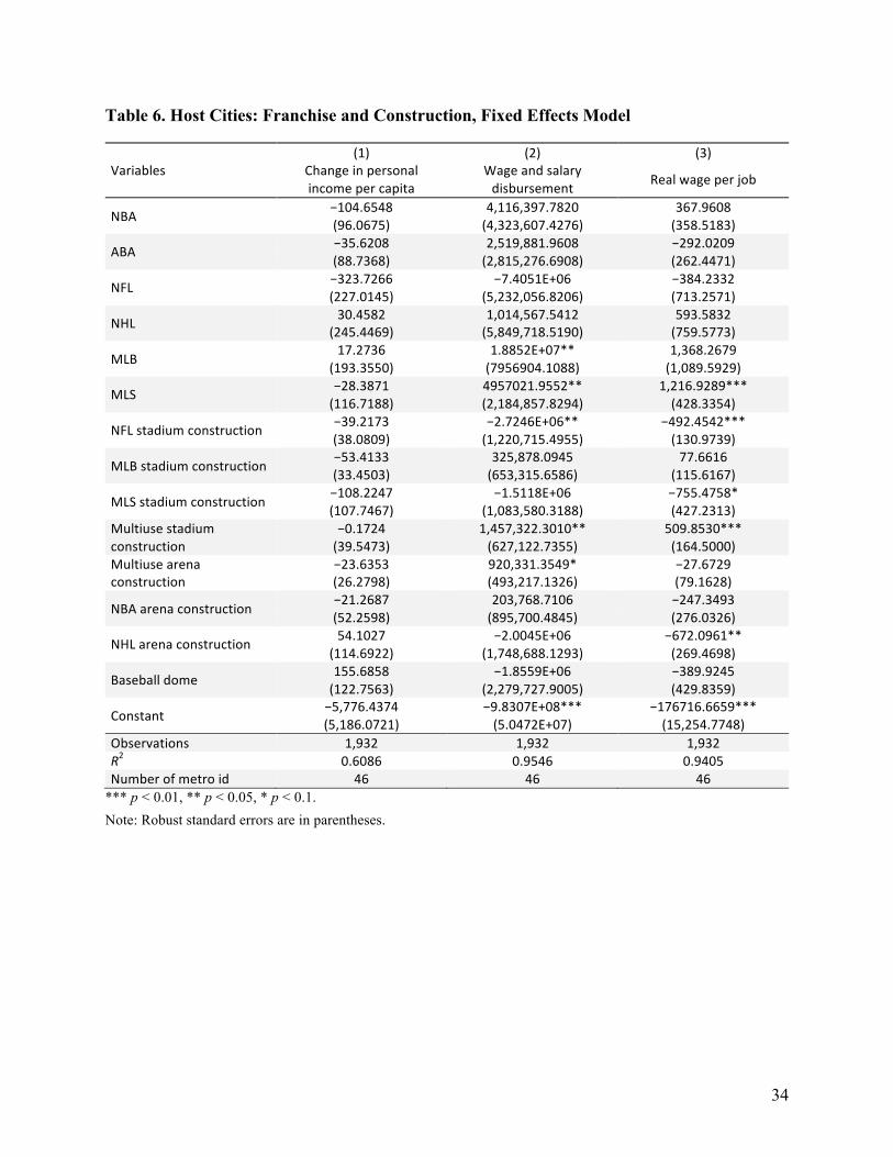
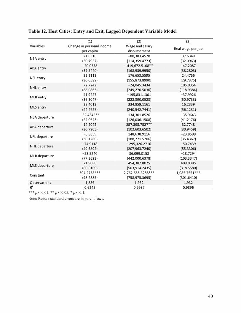
economy. Tables 6 through 13 report on subsets of coefficients; tables 6 through 9 report on
franchise presence and facility construction; and tables 10 through 13 report on entry and
departure. Tables vary by whether the sample is host cities or all cities and whether the
regression uses fixed effects or lagged dependent variables. The evidence from the individual
coefficients is mixed across specifications and samples. Many variables are not individually
significant, and they frequently have the wrong sign. It is common for them to be significant and
of the wrong sign, thus suggesting a negative relationship between sports stadiums and the
measure of income.
Stadium advocates often point to the facility as anchoring other development (Chema
1996; Santo 2005; Austrian and Rosentraub 2002; Nelson 2002). For example, a facility serves
as the main attraction for attendance at the sporting events or at concerts and other types of
entertainment, thereby providing an opportunity for other establishments to open or expand in
the neighborhood. To assess this possibility, one must consider the effect over the first 10 years
after construction of stadium or arena openings on the MSA. Whether the model is estimated
with fixed effects or the lagged dependent variable, when all three possible dependent variables
are taken into account, only 7 of 42 stadium construction coefficients are individually
statistically significant at the 10 percent level or better in the host-city sample. All seven of these
coefficients come from the fixed effects specification; none comes from the lagged dependent
variable models. Interestingly, four of the seven are negative. If one looks only at point estimates
and not at individual significance, 16 of 21 stadium or arena construction variables have negative
signs in the lagged dependent variable models, and 14 of 21 have negative signs in the fixed
effects specifications. Given these findings, the hypothesis that construction of a stadium or
21
arena fosters the local economic development that construction advocates claim has little
support. Nonetheless, perhaps comparing host cities to host cities is inappropriate; perhaps the
better comparison is between host cities and nonhost cities.
In the full sample, with the lagged dependent variable as a regressor, 4 of 21 construction
variables are individually significant at the 10 percent level or better. All four carry negative
signs, and three of them relate to the NFL stadium construction. In the fixed effects specification,
7 of 21 construction variables have a statistically significant coefficient, and 4 are negative. If
one looks only at point estimates and not at individual statistical significance, 13 of 21
coefficients are negative in the fixed effects specifications, and 14 are negative in the lagged
dependent variable models. The evidence of a positive sign is a bit stronger in the full sample, in
which hosts are compared to nonhosts, but the results still suggest construction has very little
influence on personal income per capita, wage and salary distributions, or wages per job.
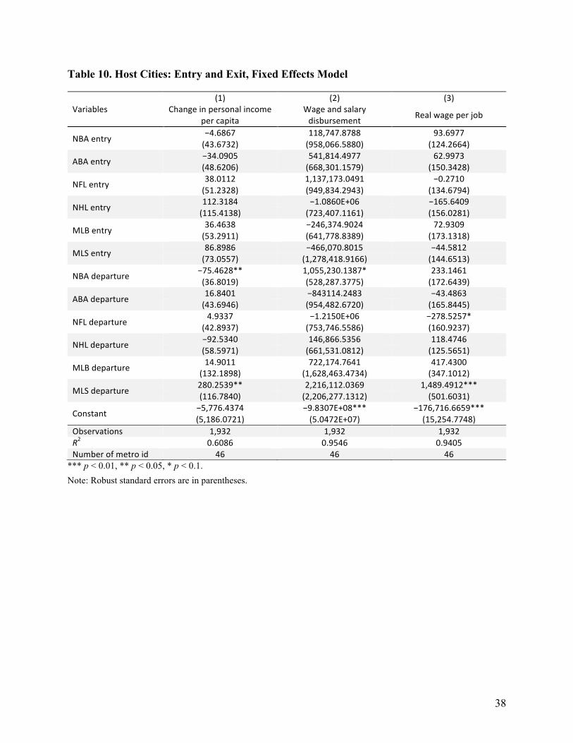
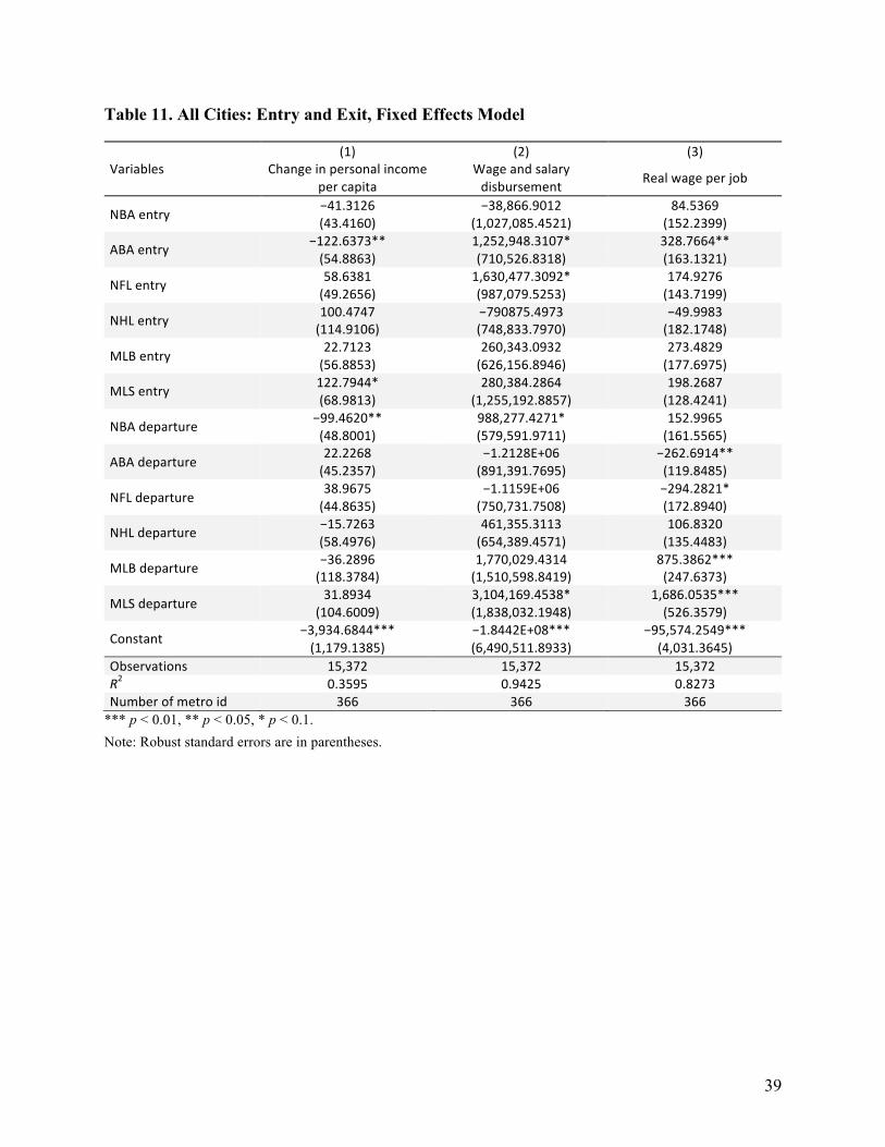
Advocates of stadium and arena construction often promote these policies as an attempt
to attract a franchise or to keep an existing franchise from moving. The regression models
include variables indicating the arrival or departure of a franchise. Support for sports as
economic development would come in the form of positive effects of franchise entry or negative
effects of franchise departure, or both. Tables 10 through 13 report the coefficients on these entry
and exit variables for each sample, host cities or all cities; for each of the three dependent
variables; and for each specification, either fixed effects of lagged dependent variables. Each
table has 18 franchise entry variables. These variables capture the effect of a new franchise in a
city in each of the first 10 years after the arrival of the franchise. In the host-city sample, only 1
of 36 entry variables is individually statistically significant, and that variable shows a negative
effect for the entry of an ABA franchise on wage and salary disbursements. Among the point

22
estimates, seven entry variables have a negative sign in the lagged dependent variable equation,
and eight are negative in the fixed effects specification. The lack of individually significant
coefficient estimates suggests that entry of franchises has no effect on personal income per
capita, wage and salary distributions, and wages per job when host cities are compared to other
host cities. Regarding the full sample, more support exists for the positive effects of franchise
entry. In the fixed effects specification, five individual coefficients are significant at the 10
percent level or better, and four of those are positive. In the model with the lagged dependent
variable, six individual coefficients are significant: three are positive, and three are negative. All
of the negative coefficients relate to entry of an ABA franchise.
Over the run of the sample period, numerous franchises left one city for another. Dummy
variables capture the effect of these departures over the first 10 years after the team leaves town.
When fixed effects are used on the host-city sample, two of the five individually statistically
significant departure variables have a negative sign, as would be the case if a franchise leaving
town harmed the local economy. But three of those five have positive coefficients: departure of a
franchise was beneficial in personal income per capita, wage and salary disbursements, or wages
per job. In the lagged dependent variable models, only two coefficients are individually
significant—one positive and one negative. Regarding the full sample with fixed effects, three of
seven individually significant variables have negative signs; in the lagged dependent variable
model only four variables are individually significant—two for each sign. The effect of franchise
departure, given these results, is negligible, with a slight suggestion that a team leaving is
beneficial in the various measures of income.
The final issue addressed is the contribution of sports to the local economy. Because
groups of coefficients are jointly significant even though very few coefficients are individually

23
significant, the overall contribution of sports to personal income per capita, wage and salary
disbursements, or wages per job is calculated. Using the coefficients from the various models,
one may compute the fitted portion of the dependent variable for each observation. The fitted
portion is split into the contribution of sports and the contribution of everything else. Tables 14
and 15 (pages 42 and 43) report on these contributions: table 14 for the host sample and table 15
for the full sample. Looking first at the host-city sample, one sees that sports appear to make an
enormous contribution to personal income per capita as the sports share is 0.22. That is, on
average, a sport’s contribution to personal income per capita is about 22 percent in the fixed
effects model. However, this finding is misleading because this large value occurs in a model
where the sports variables are not jointly statistically significant. In those cases where the sports
environment variables are jointly significant, the sports contribution is generally quite small,
with the largest contribution reaching only 4 percent. The results are much the same for the full
sample of cities, except that no sports contribution exceeds 5 percent.
VI. Conclusion
The question of whether and to what extent the sports environment affects local economies has
been discussed for years. Coates and Humphreys (1999) built on and extended existing work on
the issue by pooling data from cities that hosted franchises in one or more of the NFL, NBA, and
MLB over the period 1969–1996. Their evidence was that the overall effect of the sports
environment was to reduce personal income per capita by a small amount. The current study
updates Coates and Humphreys’s analysis by extending the sample to include 1997–2011,
incorporating both host and nonhost cities, and including the NHL and MLS in the analysis. Its
findings are similar to the earlier findings. Specifically, the sports environment is a statistically

24
significant factor in explaining personal income per capita, wage and salary disbursements, and
wages per job. As in Coates and Humphreys (1999), few variables are individually statistically
significant, and those that are often have the wrong sign. In other words, many of the individual
coefficients are opposite to what proponents of stadium- and arena-led development would have
hypothesized. That is, effects that proponents argue will be positive, such as stadium or arena
construction and attracting a franchise, are frequently negative. Even when positive, these effects
are generally quite small.
The results of using the models to forecast the contribution sports make to personal
income per capita, wage and salary disbursements, and wages per job indicate sports play a role,
but that role is small. The largest contribution sports have is less than 5 percent. As big as people
perceive sports to be, the evidence here suggests sports franchises, stadium construction, and the
other aspects of the sports environment, account for less than 5 percent of the economy, with
most estimates under 1.5 percent and some even negative, on average.
Overall, the results here are consistent with and confirm the findings of Coates and
Humphreys (1999) that sports-led development is unlikely to succeed in making a community
richer. If the local government is looking for a policy to foster economic growth, far better
candidate policies exist than those subsidizing a professional sports franchise.

25
References
Ahlfeldt, G., and W. Maennig. 2012. “Voting on a NIMBY Facility: Proximity Cost of an ‘Iconic’ Stadium.” Urban Affairs Review 48 (2): 205–37.
Angrist, J., and J.-S. Pischke. 2008. Mostly Harmless Econometrics. Princeton, NJ: Princeton University Press.
Austrian, Z., and M. S. Rosentraub. 2002. “Cities, Sports, and Economic Change: A Retrospective Assessment.” Journal of Urban Affairs 24 (5): 549–63.
Baade, R. 1996. “Professional Sports as Catalysts for Metropolitan Economic Development.” Journal of Urban Affairs 18 (1): 1–17.
Baade, R. A., R. Baumann, and V. A. Matheson. 2008. “Selling the Game: Estimating the Impact of Professional Sports through Taxable Sales.” Southern Economic Journal 74 (3): 794–810.
———. 2011. “Big Men on Campus: Estimating the Economic Impact of College Sports on Local Economies.” Regional Studies 45 (3): 371–80.
Baade, R. A., and R. F. Dye. 1988. “An Analysis of the Economic Rationale for Public Subsidization of Sports Stadiums.” Annals of Regional Science 22 (2): 37–47.
———. 1990. “The Impact of Stadiums and Professional Sports on Metropolitan Area Development.” Growth and Change 21 (2): 1–14.
Baade, R. A., and V. A. Matheson. 2000. “High Octane? Grading the Economic Impact of the Daytona 500.” Marquette Sports Law Journal 10 (2): 401–15.
———. 2001. “Home Run or Wild Pitch? The Economic Impact of Major League Baseball’s All-Star Game on Host Cities.” Journal of Sports Economics 2 (4): 307–26.
———. 2004a. “The Quest for the Cup: Assessing the Economic Impact of the World Cup.” Regional Studies 38 (4): 343–54.
———. 2004b. “An Economic Slam Dunk or March Madness? Assessing the Economic Impact of the NCAA Basketball Tournament.” In Economics of College Sports, edited by John Fizel and Rodney Fort, 111–33. Westport, CT: Praeger.
———. 2006. “Padding Required: Assessing the Economic Impact of the Super Bowl.” European Sports Management Quarterly 6 (4): 353–74.
Cantor, M., and M. Rosentraub. 2012. “A Ballpark and Neighborhood Change: Economic Integration, a Recession, and the Altered Demography of San Diego’s Ballpark District after Eight Years.” City, Culture, and Society 3 (3): 219–26.

26
Carlino, G., and N. E. Coulson. 2004. “Compensating Differentials and the Social Benefits of the NFL.” Journal of Urban Economics 56: 25–50.
Chema, T. V. 1996. “When Professional Sports Justify the Subsidy.” Journal of Urban Affairs 18 (1): 19–22.
Coates, D. 2006. “The Tax Benefits of Hosting the Super Bowl and the MLB All-Star Game: The Houston Experience.” International Journal of Sport Finance 1 (4): 239–52.
———. 2007. “Stadiums and Arenas: Economic Development or Economic Redistribution?” Contemporary Economic Policy 25 (4): 565–77.
———. 2012. “Not-so-Mega Events.” In International Handbook of Economics of Mega Sporting Events, edited by A. Zimbalist and W. Maennig. Cheltenham, UK: Edward Elgar.
———. 2013. “The Economic Impact of the Women’s World Cup.” In Handbook on the Economics of Women’s Sports, edited by E. M. Leeds and M. Leeds. Cheltenham, UK: Edward Elgar.
Coates, D., and C. Depken. 2009. “Do College Football Games Pay for Themselves? The Impact of College Football Games on Local Sales Tax Revenues.” Eastern Economic Review 35 (4): 531–47.
———. 2011. “Mega-Events: Is the Texas Baylor Game to Waco What the Super Bowl Is to Houston?” Journal of Sports Economics 12 (6): 599–620.
Coates, D., and D. Gearhart. 2008. “NASCAR as a Public Good.” International Journal of Sport Finance 3 (1): 41–57.
Coates, D., and B. R. Humphreys. 1999. “The Growth Effects of Sports Franchises, Stadia, and Arenas.” Journal of Policy Analysis and Management 18 (4): 601–24.
———. 2001. “The Economic Consequences of Professional Sports Strikes and Lockouts.” Southern Economic Journal 67 (3): 737–47.
———. 2002. “The Economic Impact of Postseason Play in Professional Sports.” Journal of Sports Economics 3 (3): 291–99.
———. 2003. “The Effect of Professional Sports on Earnings and Employment in the Services and Retail Sectors in US Cities.” Regional Science and Urban Economics 33: 175–98.
———. 2006. “Proximity Benefits and Voting on Stadium and Arena Subsidies.” Journal of Urban Economics 59 (2): 285–99.
———. 2008. “Do Economists Reach a Conclusion for Sports Franchises, Stadiums, and Mega-Events?” Econ Journal Watch 5 (3): 294–315.
27
———. 2011. “The Effect of Professional Sports on the Earnings of Individuals: Evidence from Microeconomic Data.” Applied Economics 43 (29): 4,449–59.
Coates, D., B. R. Humphreys, and A. Zimbalist. 2006. “Compensating Differentials and the Social Benefits of the NFL: A Comment.” Journal of Urban Economics 60 (1): 124–31.
Coates, D., and V. Matheson. 2011. “Mega-Events and Housing Costs: Raising the Rent while Raising the Roof?” Annals of Regional Science 46 (1): 119–37.
Davis, M., and C. End. 2010. “A Winning Proposition: The Economic Impact of Successful NFL Franchises.” Economic Inquiry 48 (1): 39–50.
Feddersen, A., and W. Maennig. 2013. “Mega-Events and Sectoral Employment: The Case of the 1996 Olympic Games.” Contemporary Economic Policy 31 (3): 580–603.
Feng, X., and B. R. Humphreys. 2008. “Assessing the Economic Impact of Sports Facilities on Residential Property Values: A Spatial Hedonic Approach” Working Paper 0812, International Association of Sports Economists, Limoges, France.
Gius, M., and D. Johnson. 2001. “An Empirical Estimation of the Economic Impact of Major League Sports Teams on Cities.” Journal of Business and Economic Studies 7 (1): 32–38.
Hotchkiss, J. L., R. E. Moore, and S. M. Zobay. 2003. “Impact of the 1996 Summer Olympic Games on Employment and Wages in Georgia.” Southern Economic Journal 69 (3): 691–704.
Humphreys, B. R., and X. Feng. 2012. “The Impact of Professional Sports Facilities on Housing Values: Evidence from Census Block Group Data.” City, Culture, and Society 3 (3): 189–200.
Im, K., M. Pesharan, and Y. Shin. 2003. “Testing for Unit Roots in Heterogeneous Panels.” Journal of Econometrics 115 (1): 53–74.
Lavoie, M., and G. Rodríguez. 2005. “The Economic Impact of Professional Teams on Monthly Hotel Occupancy Rates of Canadian Cities: A Box-Jenkins Approach.” Journal of Sports Economics 6 (3): 314–24.
Leeds, M. A. 2007. “Do Good Olympics Make Good Neighbors?” Contemporary Economic Policy 26 (3): 460–67.
Lertwachara, K., and J. Cochran. 2007. “An Event Study of the Economic Impact of Professional Sport Franchises on Local US Economies.” Journal of Sports Economics 8 (3): 244–54.
Madden, J. R. 2006. “Economic and Fiscal Impacts of Mega Sporting Events: A General Equilibrium Assessment.” Public Finance and Management 6 (3): 346.
Matheson, V. 2005. “Contrary Evidence on the Impact of the Super Bowl on the Victorious City.” Journal of Sports Economics 6 (4): 420–28.

28
Miller, P. A. 2002. “The Economic Impact of Sports Stadium Construction: The Case of the Construction Industry in St. Louis, MO.” Journal of Urban Affairs 24 (2): 159–73.
Nelson, A. C. 2001. “Prosperity or Blight? A Question of Major League Stadia Locations.” Economic Development Quarterly 15 (3): 255–65.
———. 2002. “Locating Major League Stadiums Where They Can Make a Difference: Empirical Analysis with Implications for All Major Public Venues.” Public Works Management and Policy 7 (2): 98–114.
Porter, P. K. 1999. “Mega-Sports Events as Municipal Investments: A Critique of Impact Analysis.” In Sports Economics: Current Research, edited by J. Fizel, E. Gustafson, and L. Hadley, 61–74. Westport, CT: Praeger.
Porter, P. K., and D. Fletcher. 2008. “The Economic Impact of the Olympic Games: Ex Ante Predictions and Ex Poste Reality.” Journal of Sport Management 22 (4): 470–86.
Rappaport, J., and C. Wilkerson. 2001. “What Are the Benefits of Hosting a Major League Sports Franchise?” Economic Review 86 (1): 55–86.
Rosentraub, M. 2006. “The Local Context of a Sports Strategy for Economic Development.” Urban Studies 20 (3): 278–91.
Santo, C. 2005. “The Economic Impact of Sports Stadiums: Recasting the Analysis in Context.” Journal of Urban Affairs 27 (2): 177–91.
Siegfried, J., and A. Zimbalist. 2000. “The Economics of Sports Facilities and Their Communities.” Journal of Economic Perspectives 14 (3): 95–114.
———. 2006. “Policy Forum: Economics of Sport: The Economic Impact of Sports Facilities, Teams, and Mega-Events.” Australian Economic Review 39 (4): 420–27.
Tu, C. C. 2005. “How Does a Sports Stadium Affect Housing Values? The Case of FedEx Field.” Land Economics 81 (3): 379–95.
Wassmer, R. W. 2001. “Metropolitan Prosperity from Major League Sports in the CBD: Stadia Locations or Just Strength of the Central City? A Reply to Arthur Nelson.” Economic Development Quarterly 15 (3): 266–71.
Zipp, J. F. 1996. “The Economic Impact of the Baseball Strike of 1994.” Urban Affairs Review 32 (2): 157–85.

29
Table 1. Metropolitan Statistical Areas Hosting at Least One Professional Sports Franchise
Atlanta–Sandy Springs–Marietta, GA Milwaukee–Waukesha–West Allis, WI
Baltimore–Towson, MD Minneapolis–St. Paul–Bloomington, MN–WI
Boston–Cambridge–Quincy, MA–NH Nashville–Davidson–Murfreesboro–Franklin, TN Buffalo–Niagara Falls, NY New Orleans–Metairie–Kenner, LA
Charlotte–Gastonia–Rock Hill, NC–SC New York–Northern New Jersey–Long Island, NY–NJ–PA Chicago–Joliet–Naperville, IL–IN–WI Oklahoma City, OK
Cincinnati–Middletown, OH–KY–IN Orlando–Kissimmee–Sanford, FL
Cleveland–Elyria–Mentor, OH Philadelphia–Camden–Wilmington, PA–NJ–DE–MD Columbus, OH Phoenix–Mesa–Glendale, AZ
Dallas–Fort Worth–Arlington, TX Pittsburgh, PA Denver–Aurora–Broomfield, CO Portland–Vancouver–Hillsboro, OR–WA
Detroit–Warren–Livonia, MI Raleigh–Cary, NC Green Bay, WI Sacramento–Arden–Arcade–Roseville, CA
Greensboro–High Point, NC Salt Lake City, UT
Hartford–West Hartford–East Hartford, CT San Antonio–New Braunfels, TX Houston–Sugar Land–Baytown, TX San Diego–Carlsbad–San Marcos, CA
Indianapolis–Carmel, IN San Diego–Carlsbad–San Marcos, CA Jacksonville, FL San Jose–Sunnyvale–Santa Clara, CA
Kansas City, MO–KS Seattle–Tacoma–Bellevue, WA
Los Angeles–Long Beach–Santa Ana, CA St. Louis, MO–IL Louisville–Jefferson County, KY–IN Tampa–St. Petersburg–Clearwater, FL
Memphis, TN–MS–AR Virginia Beach–Norfolk–Newport News, VA Miami–Fort Lauderdale–Pompano Beach, FL Washington–Arlington–Alexandria, DC–VA–MD–WV
30
Table 2. Host-City and Full Sample Wage and Income Variables
Observations Mean Standard deviation Minimum Maximum
Host-‐city sample
Personal income per capita 1,978 $15,750.44 3,660.707 $8,509.54 $31,814.75 Growth rate of personal income per capita 1,932 0.0141 0.0006 n.a. n.a.
Wage and salary disbursement 1,978 2.82E+07 3.46E+07 1,162,520 2.75E+08
Growth rate of wage and salary disbursement 1,932 0.0216 0.0008 n.a. n.a.
Wage per job 1,978 19,648.12 3,245.565 14,324.5 43,172.48 Growth rate of wage per job 1,932 0.0053 0.0005 n.a. n.a.
Full sample
Personal income per capita 15,738 $13,399.46 3,292.067 $4,803.81 $38,650.64 Growth rate of personal income per capita 15,372 0.0136 0.0002 n.a. n.a.
Wage and salary disbursement
15,738 5,258,417 1.52E+07 15,561.3 2.75E+08
Growth rate of wage and salary disbursement
15,372 0.0197 0.0003 n.a. n.a.
Wage per job 15,738 $16,825.66 2,661.983 $10,926.4 $43,172.48
Growth rate of wage per job 15,372 0.0033 0.0005 n.a. n.a. Note: n.a. = not applicable.

31
Table 3. Im, Pesharan, and Shin (2003) Panel Unit Root Tests
Full sample Host sample
One lag Two lags Three lags One lag Two lags Three lags
Levels Wage and salary yes yes yes yes yes yes
Wage per job no no yes 10% 10% yes
Personal income per capita no no no no no no
Logs
Wage and salary yes yes yes yes no yes
Wage per job no no yes no no no Personal income per capita growth rate
no no no no no no
Wage and salary yes yes yes yes yes yes
Wage per job yes yes yes yes yes yes
Personal income per capita yes yes yes yes yes yes Note: All models include a trend.
32
Table 4. Joint Hypothesis Tests: Host Cities
Personal income per
capita Wage disbursement Wages per job
Fixed effects model
Regression f(127,1759) = 21.5 f(127,1759) = 291.2 f(127,1759) = 218.8
p = 0.000 p = 0.000 p = 0.000
Sports f(40,1759) = 1.19 f(40,1759) = 14.25 f(40,1759) = 9.50
p = 0.194 p = 0.000 p = 0.000
Franchise f(6,1759) = 0.50 f(6,1759) = 20.86 f(6,1759) = 8.28
p = 0.808 p = 0.000 p = 0.000
and capacity f(16,1759) = 1.47 f(16,1759) = 17.38 f(16,1759) = 8.76
p = 0.102 p = 0.000 p = 0.000
and entry and exit f(28,1759) = 1.45 f(28,1759) = 15.13 f(28,1759) = 9.53
p = 0.061 p = 0.000 p = 0.000
and construction f(36,1759) = 1.26 f(36,1759) = 15.45 f(36,1759) = 10.49
p = 0.144 p = 0.000 p = 0.000
Olympic host f(4,1759) = 0.52 f(4,1759) = 5.11 f(4,1759) = 0.51
p = 0.723 p = 0.000 p = 0.728
Lagged dependent variable model
Regression f(127,1758) = 23.0 f(128, 1803) = 11062 f(128, 1803) = 1342.6
p = 0.000 p = 0.000 p = 0.000
Sports f(35,1758) = 0.85 f(35,1803) = 3.41 f(35,1803) = 1.86
p = 0.714 p = 0.000 p = 0.002
Franchise f(6,1758) = 0.63 f(6,1803) = 3.86 f(6,1803) = 1.88
p = 0.704 p = 0.001 p = 0.081
and capacity f(11,1758) = 1.47 f(11,1803) = 6.03 f(11,1803) = 3.32
p = 0.135 p = 0.000 p = 0.000
and entry and exit f(23,1758) = 1.02 f(23,1803) = 4.02 f(23,1803) = 2.63
p = 0.439 p = 0.000 p = 0.000
and construction f(31,1758) = 0.89 f(31,1803) = 3.11 f(31,1803) = 2.06
p = 0.645 p = 0.000 p = 0.001
Olympic host f(4,1758) = 0.52 f(4,1803) = 3.11 f(4,1803) = 0.04
p = 0.719 p = 0.015 p = 0.997

33
Table 5. Joint Hypothesis Tests: Full Sample
Personal income per capita Wage disbursement Wages per job
Fixed effects model
Regression f(447,14559) = 18.28 f(447,14559) = 534.1 f(447,14559) = 156.0
p = 0.000 p = 0.000 p = 0.000
Sports f(40,14559) = 1.82 f(40,14559) = 137.7 f(40,14559) = 15.78
p = 0.001 p = 0.000 p = 0.000
Franchise f(6,14559) = 1.34 f(6,14559) = 179.87 f(6,14559) = 8.32
p = 0.236 p = 0.000 p = 0.000
and capacity f(16,14559) = 1.39 f(16,14559) = 135.43 f(16,14559) = 9.37
p = 0.138 p = 0.000 p = 0.000
and entry and exit
f(28,14559) = 1.87 f(28,14559) = 154.5 f(28,14559) = 16.97
p = 0.004 p = 0.000 p = 0.000
and construction f(36,14559) = 1.90 f(36,14559) = 150.0 f(36,14559) = 117.44
p = 0.001 p = 0.000 p = 0.000
Olympic host f(4,14559) = 0.88 f(4,14559) = 52.5 f(4,14559) = 3.15
p = 0.476 p = 0.000 p = 0.014
Lagged dependent variable model
Regression f(447,14558) = 18.63 f(448,14923) = 29819.4 f(448,14923)= 2441.2
p = 0.000 p = 0.000 p = 0.000
Sports f(35,14558) = 1.41 f(35,14923) = 29.2 f(35,14923) = 3.30
p = 0.053 p = 0.000 p = 0.000
Franchise f(6,14558) = 0.90 f(6,14923) = 20.87 f(6,14923) = 1.18
p = 0.492 p = 0.000 p = 0.314
and capacity f(11,14558) = 1.40 f(11,14923) = 40.7 f(11,14923) = 4.15
p = 0.167 p = 0.000 p = 0.000
and entry and exit
f(23,14558) = 1.53 f(23,14923) = 32.88 f(23,14923) = 4.52 p = 0.051 p = 0.000 p = 0.000
and construction f(31,14558) = 1.48 f(31,14923) = 25.52 f(31,14923) = 3.63
p = 0.043 p = 0.000 p = 0.000
Olympic host f(4,14558) = 0.79 f(4,14923) = 30.71 f(4,14923) = 0.16
p = 0.533 p = 0.000 p = 0.961
34
Table 6. Host Cities: Franchise and Construction, Fixed Effects Model
Variables (1) (2) (3)
Change in personal income per capita
Wage and salary disbursement Real wage per job
NBA −104.6548 4,116,397.7820 367.9608 (96.0675) (4,323,607.4276) (358.5183)
ABA −35.6208 2,519,881.9608 −292.0209 (88.7368) (2,815,276.6908) (262.4471)
NFL −323.7266 −7.4051E+06 −384.2332 (227.0145) (5,232,056.8206) (713.2571)
NHL 30.4582 1,014,567.5412 593.5832 (245.4469) (5,849,718.5190) (759.5773)
MLB 17.2736 1.8852E+07** 1,368.2679
(193.3550) (7956904.1088) (1,089.5929)
MLS −28.3871 4957021.9552** 1,216.9289*** (116.7188) (2,184,857.8294) (428.3354)
NFL stadium construction −39.2173 −2.7246E+06** −492.4542*** (38.0809) (1,220,715.4955) (130.9739)
MLB stadium construction −53.4133 325,878.0945 77.6616 (33.4503) (653,315.6586) (115.6167)
MLS stadium construction −108.2247 −1.5118E+06 −755.4758* (107.7467) (1,083,580.3188) (427.2313)
Multiuse stadium construction
−0.1724 1,457,322.3010** 509.8530*** (39.5473) (627,122.7355) (164.5000)
Multiuse arena construction
−23.6353 920,331.3549* −27.6729 (26.2798) (493,217.1326) (79.1628)
NBA arena construction −21.2687 203,768.7106 −247.3493 (52.2598) (895,700.4845) (276.0326)
NHL arena construction 54.1027 −2.0045E+06 −672.0961** (114.6922) (1,748,688.1293) (269.4698)
Baseball dome 155.6858 −1.8559E+06 −389.9245 (122.7563) (2,279,727.9005) (429.8359)
Constant −5,776.4374 −9.8307E+08*** −176716.6659*** (5,186.0721) (5.0472E+07) (15,254.7748)
Observations 1,932 1,932 1,932 R2 0.6086 0.9546 0.9405 Number of metro id 46 46 46
*** p < 0.01, ** p < 0.05, * p < 0.1. Note: Robust standard errors are in parentheses.

35
Table 7. Full Sample: Franchise and Construction, Fixed Effects Model
Variables (1) (2) (3)
Change in personal income per capita
Wage and salary disbursement Real wage per job
NBA −133.5486 4,634,787.4208 626.8419* (92.5807) (4,212,081.6612) (379.3705)
ABA −132.3844 3,390,477.6772 258.2765 (82.1019) (2,642,225.5819) (249.1933)
NFL −284.8153 −6.9263E+06 −108.6683 (243.2906) (5,801,641.1343) (863.6475)
NHL 132.5467 −1.7840E+06 −217.6784 (261.5995) (5644,940.0182) (986.3920)
MLB −236.7673 2.2531E+07** 2,342.0561* (183.3304) (9,340,836.6741) (1,323.7554)
MLS −293.1555** 4,328,156.4606* 1,201.2311*** (113.7559) (2,320,199.0921) (434.1128)
NFL stadium construction −67.9489* −2.0636E+06* −406.5571*** (37.9104) (1,130,450.6904) (133.5954)
MLB stadium construction −46.3573 546,861.4420 121.4057 (42.9894) (853,904.0380) (146.2311)
MLS stadium construction −48.8799 −1.1565E+06 −700.0378 (115.2357) (973,386.2990) (450.3194)
Multiuse stadium construction
−21.2795 1,525,976.3634** 596.2452*** (39.3656) (618,123.8106) (166.9907)
Multiuse arena construction
−17.3781 1,151,363.2609** 48.7499 (24.9059) (460,752.5489) (84.8248)
NBA arena construction 19.6913 −524664.0138 −488.0831 (37.2045) (1,241,377.6178) (344.2237)
NHL arena construction 164.0710 −1.3714E+06 −516.9803* (123.1811) (2,281,492.6010) (305.6530)
Baseball dome 237.3557*** −98,133.8088 88.3954 (90.3024) (1,768,820.0388) (193.5076)
Constant −3,934.6844*** −1.8442E+08*** −95,574.2549*** (1,179.1385) (6,490,511.8933) (4,031.3645)
Observations 15,372 15,372 15,372 R2 0.3595 0.9425 0.8273 Number of metro id 366 366 366
*** p < 0.01, ** p < 0.05, * p < 0.1. Note: Robust standard errors are in parentheses.

36
Table 8. Host Cities: Franchise and Construction, Lagged Dependent Variable Model
Variables (1) (2) (3)
Change in personal income per capita
Wage and salary disbursement Real wage per job
NBA −91.2054 −216911.7939 −33.0507 (74.7954) (314,134.9208) (91.4077)
ABA −21.1855 223,617.1503 75.1185 (71.8285) (266,885.1259) (95.2229)
NFL −249.6373** −2.6364E+06* 79.0023 (117.9079) (1,319,529.2371) (211.3031)
NHL 13.1806 2,509,144.8501** 592.9957*** (178.8897) (1,059,814.4329) (191.4817)
MLB −91.4836 484,421.3832 −193.9534 (170.8657) (1,773,989.7584) (338.1242)
MLS 41.0601 −48,426.6547 227.5253 (87.2801) (785,732.4860) (325.1317)
NFL stadium construction −19.1025 −164,932.3617 −35.2228 (26.5484) (115,987.5612) (33.4388)
MLB stadium construction −34.9591 185,738.0177 0.6734 (29.7946) (232,837.3534) (38.5476)
MLS stadium construction −76.3969 −97,797.3659 −285.2736 (53.5602) (496,197.3908) (191.1079)
Multiuse stadium construction
−43.5103 −118,568.8394 −25.5853 (29.0448) (207,698.2468) (34.1715)
Multiuse arena construction
−23.5887 28,469.3425 −33.9389 (20.0339) (81,325.9441) (28.4705)
NBA arena construction −23.8342 −8,050.6115 −62.4136 (54.0512) (103,648.1603) (77.3830)
NHL arena construction 26.6357 255,728.5256 −147.8187 (101.3357) (352,966.8021) (127.2074)
Baseball dome 128.0214 417,183.6194 283.1062** (114.2356) (460,432.9810) (114.4332)
Constant 504.2758*** 2,762,655.3288*** 1,085.7551*** (98.2885) (758,975.3695) (301.6410)
Observations 1,886 1,932 1,932 R2 0.6245 0.9987 0.9896
*** p < 0.01, ** p < 0.05, * p < 0.1. Note: Robust standard errors are in parentheses.

37
Table 9. Full Sample: Franchise and Construction, Lagged Dependent Variable Model
Variables (1) (2) (3)
Change in personal income per capita
Wage and salary disbursement Real wage per job
NBA −108.2047 −330,949.8334 −54.3298 (73.2971) (333,906.7356) (95.7963)
ABA −45.3324 −134,724.8825 −13.9271 (67.1288) (231,947.5183) (78.2067)
NFL −160.9266 −2.7598E+06* 49.7550 (153.4618) (1,439,918.1540) (208.9894)
NHL 14.4553 1,731,453.6119* 443.7690*** (188.9810) (1,003,218.5510) (160.1628)
MLB −307.0639* 529,948.9206 −110.9532 (171.6216) (2,108,279.1332) (283.5526)
MLS −191.0844** −613,118.2299 167.4681 (92.2504) (813,112.5901) (312.7189)
NFL stadium construction −51.4471* −283,927.1402** −79.4780** (30.5569) (138,510.9029) (34.6245)
MLB stadium construction −33.9361 237,739.8880 12.3797 (37.3613) (256,856.0857) (36.2519)
MLS stadium construction −86.4304 46,770.2402 −288.3664* (66.9756) (502,456.0116) (172.1088)
Multiuse stadium construction
−47.1085 −203,940.9402 −41.5745 (36.3140) (227,557.2582) (43.3892)
Multiuse arena construction
−19.9081 102,564.1843 −16.5485 (21.3649) (88,971.8426) (25.4217)
NBA arena construction −2.6433 92,883.9612 −18.1090 (40.0138) (162,400.7381) (55.5087)
NHL arena construction 114.1454 331,210.7289 −125.2451 (101.5826) (556,715.1071) (121.9085)
Baseball dome 202.8233** 1,155,317.9488* 396.1056*** (84.9751) (592,766.0011) (86.5248)
Constant 240.7563*** −128,708.9093*** 565.2179*** (28.6380) (20,259.8463) (75.4583)
Observations 15,006 15,372 15,372 R2 0.3639 0.9989 0.9865
*** p < 0.01, ** p < 0.05, * p < 0.1. Note: Robust standard errors are in parentheses.
38
Table 10. Host Cities: Entry and Exit, Fixed Effects Model
Variables (1) (2) (3)
Change in personal income per capita
Wage and salary disbursement Real wage per job
NBA entry −4.6867 118,747.8788 93.6977 (43.6732) (958,066.5880) (124.2664)
ABA entry −34.0905 541,814.4977 62.9973 (48.6206) (668,301.1579) (150.3428)
NFL entry 38.0112 1,137,173.0491 −0.2710 (51.2328) (949,834.2943) (134.6794)
NHL entry 112.3184 −1.0860E+06 −165.6409 (115.4138) (723,407.1161) (156.0281)
MLB entry 36.4638 −246,374.9024 72.9309 (53.2911) (641,778.8389) (173.1318)
MLS entry 86.8986 −466,070.8015 −44.5812 (73.0557) (1,278,418.9166) (144.6513)
NBA departure −75.4628** 1,055,230.1387* 233.1461 (36.8019) (528,287.3775) (172.6439)
ABA departure 16.8401 −843114.2483 −43.4863 (43.6946) (954,482.6720) (165.8445)
NFL departure 4.9337 −1.2150E+06 −278.5257*
(42.8937) (753,746.5586) (160.9237)
NHL departure −92.5340 146,866.5356 118.4746 (58.5971) (661,531.0812) (125.5651)
MLB departure 14.9011 722,174.7641 417.4300 (132.1898) (1,628,463.4734) (347.1012)
MLS departure 280.2539** 2,216,112.0369 1,489.4912*** (116.7840) (2,206,277.1312) (501.6031)
Constant −5,776.4374 −9.8307E+08*** −176,716.6659*** (5,186.0721) (5.0472E+07) (15,254.7748)
Observations 1,932 1,932 1,932 R2 0.6086 0.9546 0.9405 Number of metro id 46 46 46
*** p < 0.01, ** p < 0.05, * p < 0.1. Note: Robust standard errors are in parentheses.
39
Table 11. All Cities: Entry and Exit, Fixed Effects Model
Variables (1) (2) (3)
Change in personal income per capita
Wage and salary disbursement Real wage per job
NBA entry −41.3126 −38,866.9012 84.5369 (43.4160) (1,027,085.4521) (152.2399)
ABA entry −122.6373** 1,252,948.3107* 328.7664** (54.8863) (710,526.8318) (163.1321)
NFL entry 58.6381 1,630,477.3092* 174.9276 (49.2656) (987,079.5253) (143.7199)
NHL entry 100.4747 −790875.4973 −49.9983 (114.9106) (748,833.7970) (182.1748)
MLB entry 22.7123 260,343.0932 273.4829 (56.8853) (626,156.8946) (177.6975)
MLS entry 122.7944* 280,384.2864 198.2687 (68.9813) (1,255,192.8857) (128.4241)
NBA departure −99.4620** 988,277.4271* 152.9965 (48.8001) (579,591.9711) (161.5565)
ABA departure 22.2268 −1.2128E+06 −262.6914** (45.2357) (891,391.7695) (119.8485)
NFL departure 38.9675 −1.1159E+06 −294.2821* (44.8635) (750,731.7508) (172.8940)
NHL departure −15.7263 461,355.3113 106.8320 (58.4976) (654,389.4571) (135.4483)
MLB departure −36.2896 1,770,029.4314 875.3862*** (118.3784) (1,510,598.8419) (247.6373)
MLS departure 31.8934 3,104,169.4538* 1,686.0535***
(104.6009) (1,838,032.1948) (526.3579)
Constant −3,934.6844*** −1.8442E+08*** −95,574.2549*** (1,179.1385) (6,490,511.8933) (4,031.3645)
Observations 15,372 15,372 15,372 R2 0.3595 0.9425 0.8273 Number of metro id 366 366 366
*** p < 0.01, ** p < 0.05, * p < 0.1. Note: Robust standard errors are in parentheses.
40
Table 12. Host Cities: Entry and Exit, Lagged Dependent Variable Model
Variables (1) (2) (3)
Change in personal income per capita
Wage and salary disbursement Real wage per job
NBA entry 21.8316 −80,383.4520 37.6349 (30.7937) (114,359.4773) (32.0963)
ABA entry −20.0358 −419,672.5108** −47.2087 (39.5440) (168,939.9950) (38.2803)
NFL entry 32.2113 176,653.5595 24.4756 (30.0589) (155,873.8990) (29.7375)
NHL entry 72.7242 −24,045.3434 105.0354 (88.0863) (249,270.5030) (118.9384)
MLB entry 41.9227 −195,831.1301 −37.9926 (36.3047) (222,390.0523) (50.9733)
MLS entry 38.4013 334,859.1161 16.2339 (44.4727) (240,542.7441) (56.1231)
NBA departure −62.4345** 134,301.8526 −35.9643 (24.0643) (126,036.1508) (41.2176)
ABA departure 14.2042 257,395.7527** 32.7748 (30.7905) (102,603.6502) (30.9459)
NFL departure −6.8859 148,638.9116 −23.8589 (30.1260) (188,271.5206) (35.4367)
NHL departure −74.9118 −295,326.2716 −50.7439 (49.5892) (207,963.7240) (55.3306)
MLB departure −53.5240 36,099.0158 −18.7294 (77.3623) (442,000.6378) (103.3347)
MLS departure 71.9080 454,382.8025 409.0385 (80.6160) (503,914.2435) (318.5580)
Constant 504.2758*** 2,762,655.3288*** 1,085.7551*** (98.2885) (758,975.3695) (301.6410)
Observations 1,886 1,932 1,932 R2 0.6245 0.9987 0.9896
*** p < 0.01, ** p < 0.05, * p < 0.1. Note: Robust standard errors are in parentheses.

41
Table 13. All Cities: Entry and Exit, Lagged Dependent Variable
Variables (1) (2) (3)
Change in personal income per capita
Wage and salary disbursement
Real wage per job
NBA entry −6.4600 −185,198.6608 −15.2387 (30.3345) (121,048.4867) (32.2174)
ABA entry −96.7646** −436,344.1950** −113.9804*** (40.6100) (178,832.8040) (36.2121)
NFL entry 52.8248 343,103.0973** 22.4574 (34.8344) (159,053.4946) (31.9131)
NHL entry 83.4060 −12,835.3831 89.3183 (89.0886) (243,464.8695) (118.7011)
MLB entry 43.8192 −145,979.5870 −51.0241 (39.0340) (249,235.7867) (43.7265)
MLS entry 117.6954** 477,167.6093* 68.6162 (48.0505) (267,520.8434) (50.9199)
NBA departure −97.9523*** −27,997.1268 −88.5913** (33.1212) (131,716.3735) (40.2897)
ABA departure 53.0995** 32,056.7711 −29.7364 (26.5405) (95,292.2243) (29.0117)
NFL departure 31.8598 403,040.3642* 45.5440 (40.0298) (216,194.3057) (36.2852)
NHL departure −23.6935 −157,170.3440 −24.5742 (59.1979) (215,384.4744) (66.6540)
MLB departure −62.9600 −162,153.2648 −49.8586 (52.9031) (375,259.9410) (67.5005)
MLS departure −9.3065 211,197.9538 290.9416 (77.2178) (593,772.5344) (256.9550)
Constant 240.7563*** −128,708.9093*** 565.2179*** (28.6380) (20,259.8463) (75.4583)
Observations 15,006 15,372 15,372 R2 0.3639 0.9989 0.9865
*** p < 0.01, ** p < 0.05, * p < 0.1. Note: Robust standard errors are in parentheses.

42
Table 14. Sports and Nonsports Contributions: Host Cities
Observations Mean Standard deviation Minimum Maximum Share
Personal income per capita
Fixed effects model Sports contribution 1,932 46.9603 96.99346 −231.774 573.1055 0.223168 Nonsports contribution 1,932 163.4657 371.8432 −1,614.78 2,313.909 0.776832
Total 1,932 210.426 368.3787 −1,344.38 2,353.535 Lagged dependent variable model Sports contribution 1,886 −41.0332 68.44451 −227.379 256.2837 −0.19211 Nonsports contribution
1,886 254.6213 374.1228 −1,559.24 2,469.638 1.192114
Total 1,886 213.5881 374.8935 −1,563.94 2,434.95
Wage and salary disbursement
Fixed effects model Sports contribution 1,932 1,136,268 244,4381 −9169303 1.72E+07 0.040009 Nonsports contribution
1,932 2.73E+07 3.43E+07 1,059,716 2.69E+08 0.961268
Total 1,932 2.84E+07 3.47E+07 −314,705 2.63E+08 Lagged dependent variable model Sports contribution 1,932 555,500.5 1,395,228 −890,644 1.08E+07 0.01956 Nonsports contribution
1,932 2.79E+07 3.35E+07 540,350 2.66E+08 0.982394
Total 1,932 2.84E+07 3.47E+07 161,801 2.76E+08
Wages per job
Fixed effects model Sports contribution 1,932 240.1752 485.4283 −1167.6 3,002.072 0.012202 Nonsports contribution
1,932 19,443.6 3,039.253 14,321.9 37,808.07 0.987799
Total 1,932 19,683.77 3,215.625 14,695.7 40,810.14
Lagged dependent variable model Sports contribution 1,932 −7.0904 91.34851 −299.383 644.9659 −0.00036 Nonsports contribution 1,932 19,690.86 3,215.833 14,368.7 42,751.94 1.00036
Total 1,932 19,683.77 3,243.163 14,368.7 43,033.35

43
Table 15. Sports and Nonsports Contributions
Observations Mean Standard deviation Minimum Maximum Share
Personal income per capita
Fixed effects model Sports contribution 15,372 6.80723 50.19974 −282.627 554.2646 0.039114 Nonsports contribution 15,372 167.229 263.1834 −1,106.85 1,353.827 0.960886
Total 15,372 174.036 262.3328 −1,034.24 1,388.484 Lagged dependent variable model Sports contribution 15,006 −4.18198 33.6101 −333.458 326.5678 −0.02373 Nonsports contribution
15,006 180.379 261.9213 −943.767 1,314.54 1.023734
Total 15,006 176.197 261.8191 −998.612 1,266.07
Wage and salary disbursement
Fixed effects model Sports contribution 15,372 258,286 1,254,388 −7,180,484 2.08E+07 0.048701 Nonsports contribution
15,372 5,045,262 1.46E+07 −298,094 2.69E+08 0.951299
Total 15,372 5,303,548 1.52E+07 −298,094 2.63E+08 Lagged dependent variable model Sports contribution 15,372 87,552.3 603,477.8 −894,144 1.21E+07 0.016508 Nonsports contribution
15,372 5,215,996 1.47E+07 −286,917 2.66E+08 0.983492
Total 15,372 5,303,548 1.52E+07 −286,917 2.77E+08
Wages per job
Fixed effects model Sports contribution 15,372 47.9428 257.3305 −1,372.13 3,188.936 0.002846 Nonsports contribution
15,372 16,795 2,517.368 11,151.86 37,843.65 0.997154
Total 15,372 16,843 2,597.711 11,151.86 40,893.31 Lagged dependent variable model Sports contribution 15,372 5.92267 45.06052 −272.824 574.9037 0.000352 Nonsports contribution 15,372 16,837 2,631.192 10,950.95 42,879.2 0.999649
Total 15,372 16,843 2,647.791 10,950.95 43,267.76


