GROWTH OF BOUNDARY LAYER THICKNESS AND LENGTH …ethesis.nitrkl.ac.in/6493/1/E-27.pdf · 4 14...

i

GROWTH OF BOUNDARY LAYER THICKNESS AND LENGTH

OF FULLY DEVELOPED FLOW IN OPEN CHANNEL

A Thesis submitted in partial Fulfillment of the requirement for the degree of

BACHELOR OF TECHNOLOGY

By

CHIKKAM RAMAKRISHNA BALAJI

Roll No: 110CE0347

BICHITRANANDA BEHERA

Roll No: 110CE0348

Under the guidance of

Prof. K. K. Khatua

DEPARTMENT OF CIVIL ENGINEERING

NATIONAL INSTITUTE OF TECHNOLOGY

ROURKELA

2013-14

ii

CERTIFICATE

This is to certify that the project entitled Growth of Boundary layer

thickness and Length of fully developed flow in open channel submitted by

Mr. CHIKKAM RAMAKRISHNA BALAJI (Roll No. 110CE0347)

and Mr. BICHITRANANADA BEHERA (Roll. No.110CE0348) in

partial fulfillment of the requirements for the award of Bachelor of

Technology Degree in Civil Engineering at NIT Rourkela is an authentic

work carried out by him under my supervision and guidance.

Date: Prof. K.K.Khatua

Dept. of Civil Engineering

NIT Rourkela

iii

ACKNOWLEDGEMENT

We would like to thank NIT Rourkela for giving us the opportunity to use their

resources and work in such a challenging environment.

First and foremost we take this opportunity to express our deepest sense of

gratitude to our guide Prof.K.K.Khatua for his able guidance during our project

work. This project would not have been possible without his help and the valuable

time that he has given us from his busy schedule.

We are also thankful to Ms. Sipra rani Pradhan, Ms. Saine Sikta Dash, Mrs.

Bandita Naik, and Research Scholar, of Water Resource Engineering and staff

members of the Water Resource Engineering Laboratory, for helping and guiding

us during the experiments.

CHIKKAM RAMAKRISHNA BALAJI

110CE0347

BICHITRANANDA BEHERA

110CE0348

iv

ABSTRACT

The aim of the present work was to study the growth of boundary layer thickness and length of

fully developed flow in an open channel flow which has a great applications in fields like,

hydrodynamics (ships, torpedoes, submarines), wind engineering (buildings, water towers,

bridges), aerodynamics (airplanes, rockets, projectiles), ocean engineering (buoys, breakwaters,

cables) and transportation (trucks, automobiles, cycles). Boundary layer thickness and length of

fully developed flow is crucial for solving many engineering problems such as management of

rivers and floodplains, it is important to understand the behavior of flows within compound

channels for designing of flood control, hydraulic structure, sedimentation, water management

and excavation. In pipe flow, where boundary layer thickness is equal to radius of pipe which

can be obtained easily whereas one finds difficulty in obtaining boundary layer thickness in open

channels due to the presence of free surface. This challenge motivated us to study the growth of

boundary layer thickness and length of fully developed flow in open channel flow. Experiments

were performed to measure the characteristics of a boundary layer and fully developed flow by

making use of velocity profiles developing on a rough concrete surface placed in an open

channel flow from bottom to close proximity to the free surface. Section wise velocity

measurements were made with a pitot tube-manometer combination and Acoustic Doppler

velocimeter system along the flow depth ranging from 0, 0.2h, 0.4h, 0.6h, 0.8h.

Keywords

Open channel flow

Boundary layer thickness

Developed flow

Pitot tube

ADV

1

CONTENTS

CERTIFICATE………………………………………………………………………………… i

ACKNOWLEDGEMENT…………………………………………………………………….. ii

ABSTRACT…………………………………………………………………………………… iii

List of figures………………………………………………………………………………….. iv

Chapter-1 INTRODUCTION…………………………………………………………… 6

1.1 Open Channel Flow……………………………………………………….. 6

1.2 Classification of flows in channels………………………………………. 6

1.3 Concept of Boundary layer thickness and length of fully developed flow.. 8

1.4 Objectives ……………………………………………………………….. 9

Chapter-2 LITERATURE REVIEW……………………………………………………. 10

Chapter-3 EXPERIMENTAL………………………………………………………… 14

3.1 Layout of experiment…………………………………………………… 14

2

3.2 Experimental setup……………………………………………………… 15

3.2.1 Straight Flume…………………………………………………….. 15

3.2.2 Volumetric Tank……………………………………………………17

3.2.3 Sump Well and Overhead Tank………………………………........17

3.2.4 Motor System………………………………………………............18

3.3 Instruments used…………………………………………………...…….. 18

3.3.1 Pitot Tube…………………………………………………………18

3.3.2 Acoustic Doppler Veloci-meter (ADV)…………………………. 19

3.3.3 Derivation of velocity……………………………………………. 21

3.4 Experimental …………………………………………………………… 22

3.4.1 Methods adopted……………………………..………………… 22

3.4.1.1 Longitudinal boundary layer………...…………………. 22

3.4.1.2 Transverse boundary layer………..….………………… 23

3.5 Experimental data……………………..……………….………………… 24

Chapter-4 RESULTS AND DISCUSSION…………………………………….. 31

Chapter-5 CONCLUSIONS……………………………………………………. 42

Chapter-6 REFERENCES……………………………………………………… 44

3

LIST OF FIGURES

Fig. No. Name of Figure Page No.

1 Growth of boundary layer over a flat plate 9

2 Layout of experiment 14

3 Diagram of Straight flume 15

4 Sectional view of flume 16

5 Sectional view of in bank 16

6 Diagram of Volumetric tank 17

7 Pitot Tube 19

8 Acoustic Doppler Veloci meter 20

9 Growth of boundary layer in Longitudinal direction for depth of

flow 7.1 cm

33

10 Growth of boundary layer in Transverse direction for depth of flow

7.1 cm

33


flow 5.3 cm

34


5.3 cm

34


flow 8.8 cm

35

4

14 Growth of boundary layer in Transverse direction for depth of flow 8.8 cm 35


flow 7.7 cm

36


7.7 cm

36


flow 10.4 cm

37

18 Comparison between experimental and Bauer’s theoretical values 39

19 Comparison between experimental and US Army Corps theoretical

values

40

20 Relationship between boundary layer thickness & length of fully

developed flow with depth of flow

41

5

LIST OF TABLES

Table

No.

Name of the Table Page

No.

1 Calculation of Velocity for 7.1cm Depth of Flow in longitudinal direction 24





6 Calculation of Velocity for 7.1cm Depth of Flow in transverse direction 29




10 Comparison between experimental and Bauer’s theoretical data 38

11 Comparison between experimental and US Army Corps theoretical data 40

6

CHAPTER-1

INTRODUCTION

1.1 OPEN CHANNEL FLOW

The flow of liquid with a free surface is known as open channel flow. Free surface experiences a

constant pressure such as atmospheric pressure. In open channel flow, as the pressure is

atmospheric, the flow happens under the force of gravity which means the flow is due to the

slope of the bed of the channel only.

1.2 CLASSIFICATION OF FLOWS IN CHANNEL

1. Laminar flow and turbulent flow.

2. Sub-critical, critical and super critical flow.

3. Steady flow and unsteady flow.

4. Uniform flow and non-uniform flow.

7

Laminar Flow and Turbulent Flow

The flow in open channel is said to be laminar if Reynolds number (Re) is less than 500 or 600

and if the Reynolds number is more than 2000, the flow is said to be turbulent in open channel

flow. If Re lies between 500 and 2000, the flow is considered to be in transition state.

Sub-critical, Critical and Super Critical Flow

The flow in open channel is said to be sub-critical if the Froude number (Fe) is than 1.0. The

flow is called critical if Fe = 1.0 and if Fe > 1.0, the flow is called sinusoidal.

Pre-critical or shooting or rapid or torrential.

Froude number is defined as:

Fe = V/ (g*D)1/2 …(1.1)

Where

V = Mean velocity of flow

D = Hydraulic depth of channel = A/T

A=Wetted area

T=Top width of channel.

Steady Flow and Unsteady Flow

If the flow parameters such as depth of flow, velocity of flow, rate of flow at any point in open

channel flow do not change with respect to time, the flow is said to be steady flow. If at any

8

point in open channel flow, the velocity of flow, depth of flow or rate of flow changes with

respect to time, is said to be unsteady flow.

Uniform Flow and Non-uniform Flow

If the velocity of flow, depth of flow, slope of the channel and cross-section remain constant for

a given length of the channel the flow is said to be uniform. If the velocity of flow, depth of flow

etc., for a given length of the channel does not remain constant, the flow is said to be non-

uniform flow.

1.3 CONCEPT OF FULLY DEVELOPED FLOW AND BOUNDARY LAYER

Due to the viscous shear that takes place between the layers of fluid immediately above it and the

surface, Skin friction drag will be generated. This is predominantly seen on surface of objects

that are very long in the direction of flow compared to their height. Such bodies/objects are

called STREAMLINED BODIES. Over a solid surface when a fluid flow, layer next to the

surface might become attached to it (it wets the surface). This is known as ‘no slip condition’.

The layers of fluid above the surface are moving so between the layers of the fluid shearing takes

place. The shear stress which acts between the wall and the first moving layer next to it is known

as the wall shear stress and denoted by . The result of this action is that the velocities of the

fluid u increases with height y. The distance required for the velocity to reach 99% of u, free

stream velocity is taken as the boundary layer thickness . This layer is known as BOUNDARY

LAYER and is the BOUNDARY LAYER THICKNESS.

The boundary layer, which may be laminar at the upstream end, steadily thickens up to a certain

point in the channel length Le in which the flow is called "developing flow" .Beyond this point

the flow is called "FULLY DEVELOPED FLOW."

9

When a fluid starts to flow over a rough/smooth surface the boundary layer grows from zero.

More fluid is slowed down by frictional force between the layers of fluid close to the boundary,

as it passes over a greater length. Therefore the thickness of the slower layer increases

significantly.

OBJECTIVES

Our interest in the boundary layer is that its presence greatly affects the flow through or round an

object. Some of the phenomena associated with the boundary layer, length of fully developed

flow and discuss the effect of it on open channel flow are examined.

1. Conducting experiments in determining boundary layer thickness in open channel and

pipe flow

2. Variation of boundary layer thickness due to different flow and geometry conditions in

open channel and pipe flow.

3. To study the variation of boundary layer thickness due to different laminar and turbulent

flow conditions

Figure-1

10

CHAPTER-2

LITERATURE SURVEY

Iehisa Nezu and Wolfgang Rodi (1986) had used two colors Laser Doppler Anemometer

(LDA) system with direct digital signal processing to measure the longitudinal and vertical

velocity components in fully developed flow over smooth beds. They had re-examined the law of

the wall and the velocity defect law as the log law had often been applied to open channels

without detailed verification and was found that log law strictly can be applied to the near wall

region only. The friction velocity can be evaluated accurately from velocity measurements by

applying the log-law with Von Karman constant K = 0.412 and A = 5.29 to the near-wall region.

11

M. Salih Kirkgoz (1989) had measured the velocity profiles using a laser-doppler anemometer

in a fully developed, rectangular, subcritical open channel flow on smooth and rough beds. The

"rough" surfaces, used in the experiments had average roughness heights of 1 mm, 4 mm, 8 mm,

and 12 mm and the shear velocities are determined from velocity profiles measured close to the

bed. This shows that as the wall roughness increases the calculated shear velocities determined

from the velocity profiles are in increasing tendency. The overall data represented in terms of

law-of-the-wall distribution was reasonable; however, the velocity-defect distribution was not

satisfactory. From the study of mean velocity distributions the following conclusions are drawn.

As the average uniform roughness height increases from 1 mm to 12 mm the non-

dimensional velocity distribution becomes increasingly non-uniform in the inner region

of turbulent flow.

The thickness of the inner region of flow on a "smooth" bed is about 50-60% of the entire

boundary-layer thickness. This value decreases with an increase in Reynolds number.

The corresponding boundary layer thickness and length of developed flow for different

discharge were calculated and found that

a. There is a linear relationship between the dimensionless length L/h of the

turbulent flow developing zone of open channel flow and the ratio R/F.

b. At the axis of a fully developed turbulent flow section the boundary layer extends

to the water surface if the channel aspect ratio b/h =3.

Vito Ferro and Giorgio Baiamonte(1994) had done the velocity measurement in a rectangular

flume having gravel bed for four different bed shapes, characterized from different concentration

of coarser elements and for two conditions of small and large scale roughness to establish how

the velocity profile varies with the concentration of coarse bed elements and the ratio between

the depth h and a characteristic bed diameter.

R.N.Parthasarathy and M.Muste(1994) confirmed the non-coincidence of the planes of

maximum velocity and zero Reynolds stress. Significant diffusion of momentum and kinetic

12

energy took place from rough to the smooth surface. AS the roughness of the cover was

increased; the vertical transfer of vertical velocity fluctuations of the cover was decreased,

resulting in a decrease in the sediment-suspension mechanism. The proper length scale in the

outer region was the height of the plane of zero total stress from the corresponding surface.

When the distance from each surface was normalised with the log law, and the measured stream

wise and vertical velocity fluctuations agreed with the exponential variations formulated in 1986

by Nezu and Rodi.

T. Song and W.H. Graf (1996) studied unsteady flow properties in an open channel with a

rough bed. A recently developed acoustic Doppler velocity profiler (ADVP) is used to obtain

instantaneously the flow profiles. From these measurements, using the Fourier components

method, the mean velocities, the turbulence intensities and the Reynolds-stress profile, are

obtained.

Graeme M. Smart (1999) investigated vertical profiles of turbulent stream wise velocities in

gravel bed rivers. Field measurements made at high and low flows with electronic pitot tubes

show logarithmic velocity profiles to extend over much of the flow depth. For the gravel bed

rivers studied the velocity at 0.6 of the total depth was generally a good indicator of depth-

averaged flow velocity. An unambiguous definition of flow depth is adopted to deal with

situations where the bed is uneven or moving. When hydraulic roughness Z0 is defined as a fitted

parameter of a logarithmic velocity profile, the river data indicate that the profile origin

displacement below the tops of roughness elements scales with Z0. No direct relation between Z0

and bed material size is evident under mobile bed conditions. For these conditions a relation

between hydraulic roughness and U*2 is identified (with U* also derived as a log profile

parameter). A flow resistance equation using this relation is verified by comparison with mobile

bed laboratory measurements in which U* is not fitted from velocity profiles.

13

Ram Balachandar and V. C. Patel (2002) had performed experiments to measure the

characteristics of a turbulent boundary layer developing on a rough surface for an open channel

flow at close proximity to the free surface. Stream wise velocity measurements were made with a

one component laser Doppler velocimeter system at the top of the spherical roughness elements.

Measurements at three stations downstream of the plate leading edge showed the growth of the

boundary layer on the rough wall and its interaction with the exterior open-channel flow and the

free surface. Resorting to the turbulence profile provides an alternative definition of the

boundary layer thickness.

Xingwei Chen and Yee-Meng Chiew (2004), they investigated theoretically and experimentally

the velocity distributions of turbulent open channel flow with bed suction. A velocity profile with

a slip velocity at the bed surface and an origin displacement under the bed surface is proposed

and discussed. Based on this assumption, a modified logarithmic law is derived. The measured

experimental velocity distribution verifies the accuracy of the theoretically derived profile. The

data show a significant increase in the near bed velocity and a velocity reduction near the water

surface, resulting in the formation of a more uniform velocity distribution. The values of the

origin displacement slip velocity and shear velocity are found to increase with increasing relative

suction. The measured data show the occurrence of two flow regions in the suction zone: a

transitional region in which the velocity readjusts rapidly; and an ‘‘equilibrium’’ region.

14

CHAPTER-3

3.1 Layout of experiment

Figure-2

Volumetric Tank

Straight Flume

Overhead tank

Over Head tank

Sump Well

Motor pump

Water

Circulation

15

3.2 EXPERIMENTAL SETUP:

3.2.1 Straight Flume

A Flume is an open artificial channel or chute carrying a stream of water. In a way a flume is a

model of a river/canal/water body for conducting experiments and observing its behavior.

Making use of flume real conditions of rivers/canal/water bodies can be generated virtually.

Flume also helps in obtaining the parameters of river/canal/any water bodies experimentally in

laboratory.

One shouldn’t be confused with flumes and aqueducts, which are built with the goal of

transporting the water, whereas a flume would use the flowing water to transport other materials.

There are different types of flume basing on geometry or shape

1. Straight flume

2. Meandering flume

But here we are concerned with the straight flume only.

The experimental flume which is straight in shape and having a rigid bed made of cement mortar

is shown in figure-3.

Figure-3

16

Figure-4 Sectional view of flume

Figure-5 Sectional view-In bank

Construction of channel is done with the use of M15 concrete mix and finished smoothly.

12.5

17

3.2.2 Volumetric Tank

It is a tank where water is temporarily stored for discharge calculations.

Area of Volumetric Tank, A=20.928784 m2

Outlet of volumetric tank is closed and water is allowed to fill the tank. Around 20-30 minutes

later, time taken for 1 cm rise of water in volumetric tank is measured. This procedure is

repeated for 4-5 times and average time (T) is evaluated.

Volume of water collected in T sec, V= A* H = A*(1cm).

Discharge, Q=V/T

= (A*1)/T m3/s

Figure-6

3.2.3 Sump well and Overhead tank

An underground tank where water from volumetric tank is collected and stored permanently and

making use of motors pumped into overhead tank for experimental usage. Overhead is a

rectangular tank placed over a certain height from ground level. Input water of overhead tanks

comes from sump well and output from overhead tank flows to flume.

18

3.2.4 Motor System

Laboratory is equipped with 2 types of motors having capacity 1HP 2HP

1. Submergible motors

2. Priming motors

Care has to be taken such that water level in overhead tank during the experiments should be

more-less constant.

3.3 INSTRUMENTS USED:

3.3.1 Pitot tube

A Pitot-tube is a device used for measuring the velocity of flow at any point in a pipe or a

channel. Its principle is based on the fact that if the velocity of flow at a point becomes zero, the

pressure there is increased due to the conversion of kinetic energy into pressure energy.

The Pitot-tube consists of a steel tube bent at right angle. The lower end, which is bent through

90 º, is directed opposite to flow direction of the water. The kinetic energy is converted to

pressure energy so the liquid rises up in the tube, with this velocity of water at a point can be

evaluated. . Diameter of pitot tube is D=4.07 mm.

The theoretical velocity is given by:

Vth = (2gh) 1/2

Where,

h = difference of pressure head which is calculated from the manometer

The actual velocity is given by:

V = Cv(2gh)1/2

19

Cv= coefficient of pitot-tube

Figure-7

Pressure difference at various locations in a straight channel for different depth was recorded.

The data recorded was used for the further calculation of velocity distribution.

3.3.2 ADV (acoustic Doppler velocimeter)

16-MHz Micro ADV (Acoustic Doppler Velocimeter) from the original Son-Tek, San Diego,

Canada, is the most significant and efficient breakthrough in 3-axis (3D) Velocity meter

Technology. The higher acoustical frequency of 16 MHz enables the Micro-ADV the optimal

instrument for laboratory-research orientated study. After setup of the Micro ADV with the

software package it is used for taking high-quality 3-D Velocity data at various points. This data

of flow area are received to the ADV-processor. Raw data after compilation by software package

of the processor is shown by the computer. For a minute, at every point the instrument records a

number of velocity data. The mean value of the point velocities (3-D) were recorded for each

flow depths using the statistical analysis using the installed software.

The Doppler shift principle is used by the Micro ADV to measure the velocity of small particles,

assumed to move at velocities similar to the fluid. Velocity is resolved into 3orthogonal

components like vertical, Tangential and radial and measured in a volume five centimeters below

20

the probe head, minimizing interference of the flow field, and allowing

measurements/observations to be made close to the bed.

The Micro ADV has the Features like

Three-axis velocity measurement

Small sampling volume -- less than 0.1 cm3

High sampling rates -- up to 50 Hz

Small optimal scattered -- excellent for low flows

Comprehensive software

Large velocity range: 1 mm/s to 2.5 m/s

High accuracy: 1% of measured range

No recalibration needed

Excellent low-flow performance

ADV (down probe) is unable to read the velocity of upper layer up to 5 cm below the free

surface so Preston tube technique in which the standard pitot tube in conjunction with a inclined

manometer is used for the measurement of point velocity readings at some specified positions for

the upper 5cm region from free surface across the channel.

Down probe Up probe

Figure-8

21

3.3.3 Derivation for velocity of flow

Velocity of flow can be calculated from Bernoulli’s equation

hg

v

g

pz

2

2

Z= Datum height

g

p

g

V

2

2

h= Total head

g

v

g

pz

g

v

g

pz

22

22

22

2

111

Here point 1 is located just outside of opening of pitot tube

Point 2 is located just before the 900 bent.

As, 021 zz

And 02 V (velocity of water inside the pitot tube is zero)

Difference in pressure heads,

sin*12 hg

P

g

P

h Height difference in manometer tubes.

= angle of inclination of manometer

Pressure head

Kinetic head

22

Therefore, sin*2

2

1 hg

V

sin2 hgV Eq. (1)

3.4 EXPERIMENTAL PROCEDURE

Evaluation of slope of flume

A long transparent thin pipe is taken and is filled with water. Desired length of channel is

selected where slope has to be evaluated with thin pipe, placed along the lengths with two ends

fixed at two points so as to make no vertical deflection of water in the thin pipe. Vertical height

difference of water in the thin pipe is measured making use of scale/tape, say A and the length

between the desired points is also measured, say B.

Slope of flume,

B

A1tan Eq. (2)

3.4.1 Method adopted

3.4.1.1 Longitudinal Boundary Layer

Water from overhead tank with a controlled discharge is allowed to flow over the surface

of channel for about 30-45 minutes for obtaining a steady flow in the channel.

Within this interval, one should make sure Pitot tube is free from bubbles. If present they

should be carefully bubbled out. Otherwise, presences of bubbles lead to erroneous

reading in manometer.

The choice of discharge should be such that overflow from main channel does not take

place.

Water level is checked with the help of needle so as to ensure constant discharge. Any

small fluctuations in the flow should be avoided for practical purposes. This may be due

to undulations in the channel bed preparations.

Channel is divided for ease in experimental approach. The division can be of 0.5m or 1m.

23

Now the setup of experiment is brought to the position where velocity profile has to be

found, say x=0 m.

Depth of flow is found by placing needle at various points (say, 5 points) in a particular

cross-section; average depth of flow in a particular cross-section is evaluated.

For obtaining rough picture of velocity profile at a section, depth of flow is divided into

five equal divisions such as 0, 0.2h, 0.4h, 0.6h, 0.8h. Reading at height H can’t be taken

as bubbles may enter into manometer.

Pitot tube is placed along the center line of section and varied from various position 0,

0.2h, 0.4h, 0.6h, 0.8h.

Readings of manometer are taken at individual depths for velocity after 3 minutes

interval of change in position of pitot tube for different depths.

From these data, h is calculated which in term gives the value of velocity at that

particular depth from eq. (1).

Above procedure is followed for next sections to find the desired boundary layer

thickness and length of fully developed flow.

3.4.1.2 TRANSVERSE BOUNDARY LAYER

Once the length of fully developed flow is known, velocity profiles of complete

transverse section are to be measured.

As Boundary layer thickness is symmetric about center line of transverse section only

half of the sections velocity profiles are measured.

Now half the length of transverse section is divided equally and named, say 321 ,, YYY etc.

The velocities at 0, 0.2h, 0.4h, 0.6h, 0.8h are measured by making use of pitot tube-

manometer combination at specified position of transverse section.

From the above data velocity profiles of transverse section to be drawn and Growth of

boundary layer thickness along the transverse can also be found out.

24

3.5 EXPERIMENTAL DATA:

FOR LONGITUDINAL DIRECTION (ALONG THE FLOW)

TABLE-1

For depth of flow=7.1cm, 07.28

X(in m) Y(in cm) H1(cm) H2(cm) H (cm) sin2 hgV

(in m/s)

2 0 56.9 56.9 0 0

0.2h 56.9 59.4 2.5 0.485

0.4h 56.5 59.5 3 0.532

0.6h 56.5 59.5 3 0.532

0.8h 56.5 59.5 3 0.532

2.5 0 55.7 55.7 0 0

0.2h 55.7 58.3 2.6 0.495

0.4h 55.5 58.5 3 0.532

0.6h 55.5 58.8 3.3 0.540

0.8h 55.5 58.5 3.3 0.540

3 0 56.5 56.5 0 0

0.2h 56.4 58.9 2.5 0.485

0.4h 56.5 59.5 3 0.532

0.6h 56.5 59.5 3 0.532

0.8h 56.5 59.5 3 0.532

3.1 0 56.3 56.3 0 0

0.2h 56.4 59.4 3 0.53

0.4h 56.5 59.6 3.1 0.54

0.6h 56.5 59.8 3.3 0.56

0.8h 56.7 60.0 3.3 0.56

3.2 0 56.2 56.2 0 0

0.2h 56.4 59.3 2.9 0.52

0.4h 56.4 59.6 3.2 0.56

0.6h 56.3 59.7 3.4 0.57

0.8h 56.3 59.7 3.4 0.57

3.5 0 58.9 56.5 2.4 0

0.2h 59.6 56.5 3.1 0.54

0.4h 59.7 56.4 3.3 0.56

06h 59.6 56.2 3.4 0.57

0.8h 59.8 56.3 3.5 0.57

4 0 56.0 56.0 0 0

0.2h 56.0 59.1 3.1 0.54

0.4h 56.3 59.7 3.4 0.57

0.6h 56.2 59.8 3.6 0.58

0.8h 55.9 59.5 3.6 0.58

25

TABLE-2

For flow depth=5.3cm, 06.28

X Y H1 H2 H (cm) sin2 hgV

(in m/s)

2 0 52.1 52.1 0 0

0.2h 52.0 53.3 1.3 0.35

0.4h 52.5 54.3 1.8 0.41

0.6h 52.9 54.9 2 0.43

0.8h 52.9 54.9 2 0.43

2.5 0 51.8 51.8 0 0

0.2h 51.5 52.9 1.4 0.36

0.4h 51.9 53.3 1.4 0.36

0.6h 51.9 53.8 1.9 0.41

0.8h 52.4 54.2 2 0.42

3 0 52.0 52.0 0 0

0.2h 52.1 53.5 1.4 0.360

0.4h 52.1 53.8 1.7 0.399

0.6h 52.0 53.8 1.8 0.41

0.8h 52.0 53.8 1.8 0.41

3.3 0 51.6 51.6 0 0

0.2h 51.7 52.7 1 0.31

0.4h 51.7 52.8 1.1 0.32

0.6h 51.7 52.8 1.1 0.32

0.8h 51.6 52.8 1.2 0.335

3.4 0 51.4 51.4 0 0

0.2h 51.3 52.4 1.1 0.32

0.4h 51.3 52.5 1.2 0.335

0.6h 51.3 52.6 1.3 0.35

0.8h 51.5 52.8 1.3 0.35

3.5 0 51.1 51.1 0 0

0.2h 51.2 52.6 1.4 0.360

0.4h 51.1 52.8 1.7 0.399

0.6h 51.1 52.8 1.7 0.399

0.8h 51.0 52.8 1.8 0.399

4 0 51.2 51.2 0 0

0.2h 51.2 52.7 1.5 0.375

0.4h 51.2 52.8 1.6 0.387

0.6h 51.1 52.8 1.7 0.399

0.8h 50.9 52.7 1.8 0.41

26

TABLE-3

Flow depth= 8.8cm, 30.5


(in m/s)

2.5 0 62 62 0 0

0.2h 62 60.6 1.4 0.373

0.4h 62.1 60.5 1.6 0.399

0.6h 62.2 60.5 1.7 0.411

0.8h 62.2 60.5 1.7 0.411

3 0 62 62 0 0

0.2h 62 60.4 1.6 0.399

0.4h 62.4 60.5 1.7 0.411

0.6h 62.4 60.5 1.7 0.411

0.8h 62.5 60.6 1.7 0.411

3.3 0 62.1 62.1 0 0

0.2h 62.1 60.6 1.5 0.386

0.4h 62.3 60.6 1.7 0.411

0.6h 62.4 60.6 1.7 0.411

0.8h 62.4 60.6 1.7 0.411

3.4 0 61.9 61.9 0 0

0.2h 61.9 60.4 1.5 0.385

0.4h 62.1 60.4 1.7 0.411

0.6h 62.1 60.4 1.7 0.411

0.8h 62.2 60.5 1.7 0.411

3.5 0 62.1 62.1 0 0

0.2h 62.1 60.4 1.7 0.411

0.4h 62.2 60.3 1.9 0.435

0.6h 62.3 60.4 1.9 0.435

0.8h 62.5 60.6 1.9 0.435

4 0 62.2 62.2 0 0

0.2h 62.2 60.5 1.7 0.411

0.4h 62.1 60.1 2 0.446

06h 62.1 60.1 2 0.446

0.8h 62 60 2 0.446

27

TABLE-4

Flow depth= 7.7 cm, 30.5


(in m/s)

2 0 61.5 61.5 0 0

0.2h 61.5 59.3 2.2 0.468

0.4h 61.7 59.3 2.4 0.489

0.6h 61.9 59.3 2.6 0.509

0.8h 62 59.3 2.7 0.519

2.5 0 59 59 0 0

0.2h 61.5 59 2.5 0.499

0.4h 61.6 58.9 2.7 0.519

0.6h 61.8 58.9 2.9 0.537

0.8h 61.9 59 2.9 0.537

3 0 61.3 61.3 0 0

0.2h 61.3 59.1 2.2 0.468

0.4h 61.6 59.1 2.5 0.499

0.6h 61.7 59.1 2.6 0.509

0.8h 61.8 59.2 2.6 0.509

3.3 0 61.2 61.2 0 0

0.2h 61.2 58.9 2.3 0.479

0.4h 61.6 58.9 2.7 0.519

0.6h 61.7 58.9 2.8 0.528

0.8h 61.7 58.9 2.8 0.528

3.5 0 61.5 61.5 0 0

0.2h 61.6 59.1 2.4 0.489

0.4h 61.7 58.9 2.7 0.519

0.6h 61.7 59.1 2.8 0.528

0.8h 61.8 59.2 2.8 0.528

4 0 61.3 61.3 0 0

0.2h 61.3 58.9 2.4 0.489

0.4h 61.5 58.8 2.7 0.519

06h 61.7 58.9 2.8 0.528

0.8h 61.7 58.9 2.8 0.528

28

TABLE-5

Using Acoustic Doppler Velocimeter

X (m) Depth of Flow Velocity (m/s)

3 0 0

0.2h 0.25

0.4h 0.38

0.6h 0.38

0.8h 0.38

3.3 0 0

0.2h 0.37

0.4h 0.39

0.6h 0.39

0.8h 0.39

3.5 0 0

0.2h 0.37

0.4h 0.39

0.6h 0.39

0.8h 0.39

4 0 0

0.2h 0.37

0.4h 0.39

0.6h 0.39

0.8h 0.39

4.5 0 0

0.2h 0.38

0.4h 0.40

0.6h 0.40

0.8h 0.40

29

FOR TRANSVERSE DIRECTION AT THE POINT WHERE THE FLOW IS FULLY

DEVELOPED

TABLE-6

For depth of flow=7.1cm, 07.28

TABLE-7

For flow depth=5.3cm, 06.28

Y Depth of

flow(cm)

H2(cm) H2(cm) H (cm) sin2 hgV

(in m/s)

35 0.2h 56.3 59 2.7 0.504

0.4h 56.3 59.4 3.1 0.540

0.6h 56.3 59.6 3.3 0.557

0.8h 56.3 59.6 3.3 0.567

25 0.2h 56.4 59.1 2.7 0.504

0.4h 56.4 59.4 3 0.532

0.6h 56.4 59.5 3.1 0.54

0.8h 56.4 59.5 3.1 0.54

15 0.2h 56.4 58.9 2.5 0.485

0.4h 56.5 59.2 2.7 0.504

0.6h 56.4 59.2 2.8 0.512

0.8h 56.4 59.2 2.8 0.512

Y Depth of

flow(cm)


(in m/s)

35 0.2h 51.9 52.8 0.9 0.291

0.4h 51.9 53 1.1 0.321

0.6h 51.8 53 1.2 0.336

0.8h 51.8 53 1.2 0.336

25 0.2h 51.7 52.6 0.9 0.291

0.4h 51.7 52.7 1 0.306

0.6h 51.7 52.7 1 0.306

0.8h 51.7 52.7 1 0.306

15 0.2h 51.5 52.5 1 0.306

0.4h 51.5 52.5 1 0.306

0.6h 51.5 52.5 1 0.306

0.8h 51.6 52.6 1 0.306

30

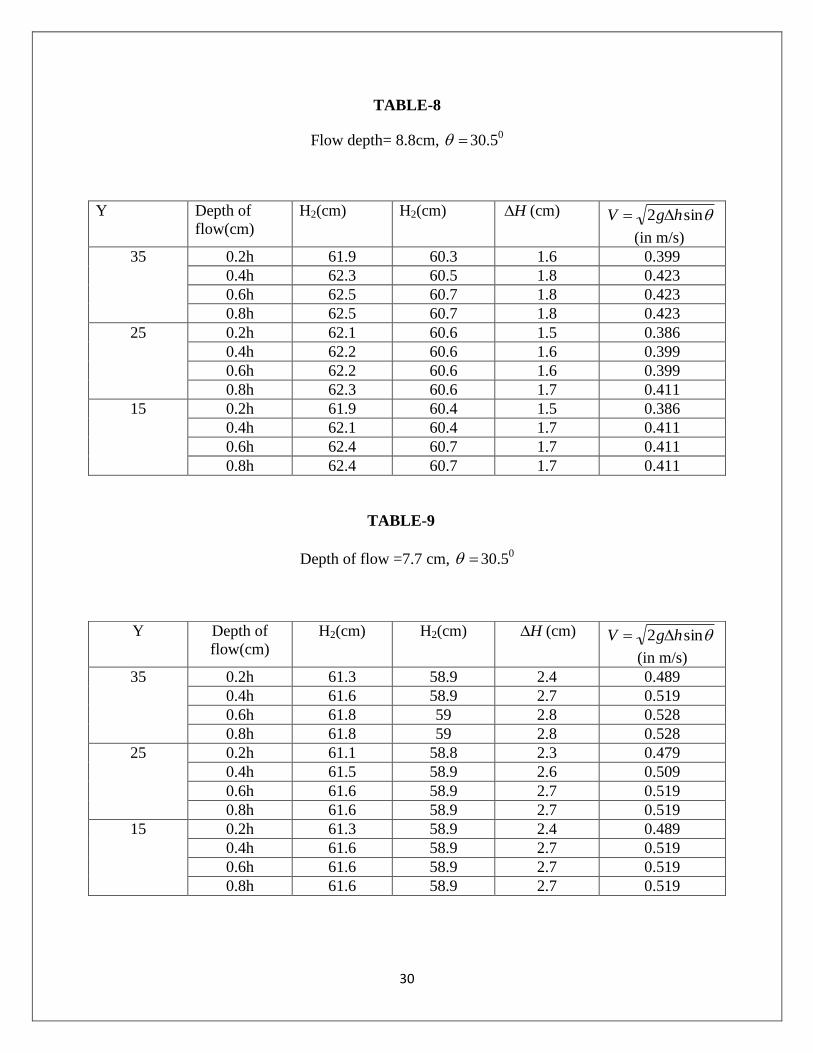
TABLE-8

Flow depth= 8.8cm, 30.50

TABLE-9

Depth of flow =7.7 cm, 30.50

Y Depth of

flow(cm)


(in m/s)

35 0.2h 61.9 60.3 1.6 0.399

0.4h 62.3 60.5 1.8 0.423

0.6h 62.5 60.7 1.8 0.423

0.8h 62.5 60.7 1.8 0.423

25 0.2h 62.1 60.6 1.5 0.386

0.4h 62.2 60.6 1.6 0.399

0.6h 62.2 60.6 1.6 0.399

0.8h 62.3 60.6 1.7 0.411

15 0.2h 61.9 60.4 1.5 0.386

0.4h 62.1 60.4 1.7 0.411

0.6h 62.4 60.7 1.7 0.411

0.8h 62.4 60.7 1.7 0.411

Y Depth of

flow(cm)


(in m/s)

35 0.2h 61.3 58.9 2.4 0.489

0.4h 61.6 58.9 2.7 0.519

0.6h 61.8 59 2.8 0.528

0.8h 61.8 59 2.8 0.528

25 0.2h 61.1 58.8 2.3 0.479

0.4h 61.5 58.9 2.6 0.509

0.6h 61.6 58.9 2.7 0.519

0.8h 61.6 58.9 2.7 0.519

15 0.2h 61.3 58.9 2.4 0.489

0.4h 61.6 58.9 2.7 0.519

0.6h 61.6 58.9 2.7 0.519

0.8h 61.6 58.9 2.7 0.519

31

CHAPTER-4

Results and discussion

As soon as observations (velocities using either pitot tube-manometer combination or ADV) are

taken, one have to tentatively find the thickness of Boundary layer at each section of

consideration.

Then by applying the definition of Boundary layer thickness i.e.., depth from bottom (rough

surface) to the point where velocity is 99% of free stream velocity.

Velocity at 99% of free stream velocity can be found out by using method of Interpolation

between two known points.

Example: Depth of flow, h=7.7

Depth Velocity

0 0

0.2h 0.489

0.4h 0.519

0.6h 0.519

0.8h 0.519

Here Free Stream velocity, V= 0.519 m/s

99% of free stream velocity, 1V = 0.99* V

1V =0.51381 m/s

So, Depth at 1V can be found by using method of Interpolation

At 0.2h depth, velocity is 0.489

At 0.4h depth, velocity is 0.519

Let Y be the depth, velocity is 0.51381

Y= hhh 2.02.04.0489.0519.0

489.051381.0

32

= hh 2.0)2.0(03.0

02481.0

= 0.1654h+0.2h =0.3654h =2.81358 cm.

For rest of Observation tables above method of interpolation is being followed.

Analysis of Results

In the graph of Boundary layer thickness in longitudinal direction, increasing trends is seen from

starting point (leaving the disturbances caused by various agents near the entrance) to length of

fully developed flow

The graph of transverse boundary layer which is being shown is only half the transverse length

of section. As the growth of Boundary layer thickness along transverse direction is symmetric

about the center-line so other half can be evaluated by taking mirror image across the center-line

of transverse section.

For rest of graphs the Growth of Boundary Layer thickness along the Transverse section is

shown from center-line to periphery i.e.., half of Transverse section.

Growth of Boundary Layer in Longitudinal direction

From the Table-1 data it is observed that the flow is fully developed after 3.1m from the entrance

of the channel. So the experimental data for the length of fully developed flow is found to be

3.1m from where the boundary layer thickness remains almost same along the direction of flow.

The thickness of the boundary layer is found to be 0.4h=2.8cm from the bottom of the channel.

Initially it is being affected by various agents but finally following the trend of increasing in the

direction of flow.

33

Figure-9

Growth of Boundary Layer in Transverse direction

At x=3.1m the velocity of flow is measured along the transverse section and the velocity profile

is given below.

Figure-10

Velocity (m/s) in X-direction


Dep

th o

f fl

ow

(cm

)

Dep

th o

f fl

ow

(cm

)

34


Boundary Layer thickness is 2.12cm for depth of flow 5.3 cm.

Figure-11


Length of fully developed flow is 3.5 m for depth of flow 5.3 cm

Figure-12


Dep

th o

f fl

ow

(cm

)


Dep

th o

f fl

ow

(cm

)

35


Boundary layer thickness is 3.2 cm for depth of flow 8.8 cm.

Figure-13


Length of fully developed flow is 3.4 m for depth of flow 8.8 cm

Figure-14

Dep

th o

f fl

ow

(cm

)


Dep

th o

f fl

ow

(cm

)


36


Boundary layer thickness 3.7 cm for depth of flow 7.7 cm

Figure-15


Length of fully developed flow is 3.3m for depth of flow =7.7 cm

Figure-16

Dep

th o

f fl

ow

(cm

)


Dep

th o

f fl

ow

(cm

)


37

Using Acoustic Doppler Veloci meter (ADV)


Boundary layer thickness is 4.2cm and length of fully developed flow is 3.3m.

Figure-17


Dep

th o

f fl

ow

(cm

)

38

COMPARISON WITH THEORITICAL VALUE

According to Bauer’s investigations (1951),

13.0

024.0

k

xx

Eq. (3)

Where =Boundary layer thickness at x

x = distance from inlet in the direction of flow where boundary layer thickness is

required.

k =roughness height (for cement surface 0.004 ft.)

Putting the respective values for x (i.e. the length of developed flow) and k the theoretical

values obtained are shown in the table.

Table-10

Discharge Length of

developed

flow( x )

Experimental value

(Boundary Layer thickness)

Theoretical value

(Boundary Layer thickness)

1 3.1m 2.8 cm 2.7 cm

2 3.5m 2.1 cm 3.0 cm

3 3.4m 3.2 cm 2.9 cm

4 3.3m 3.7 cm 2.8 cm

Here expiremental obtained are compared with theorticial values from Bauer’s equation.

39

Figure-18

From the above graph, it is observed that experimental data of boundary layer thickness obtained

increases to a maximum value and then decreases with length of fully developed flow for various

discharges (flow depths). Whereas according to Bauer’s equation there is a slight increase in

boundary layer thickness with length of fully developed flow for various discharges (flow

depths).

Similarly, from US Army Corps of engineers by Campbell et al. (1965)

233.0

08.0

sk

x

x

Eq. (4)

Where, parameters hold the same definitions as Bauer’s equation

0

0.5

1

1.5

2

2.5

3

3.5

4

3 3.1 3.2 3.3 3.4 3.5 3.6

Bo

un

dar

y la

yer

thic

kne

es

(cm

)

Length of fully developed flow for various depths (m)

Experimental Data

Bauer's theoretical Data

40

Table-11

Discharge Length of

developed flow( x )

Experimental value

(Boundary Layer

thickness)

Theoretical value

(Boundary Layer

thickness)

1 3.1 m 2.8 cm 3.9

2 3.5 m 2.1 cm 4.3

3 3.4 m 3.2 cm 4.2

4 3.3 m 3.7 cm 4.1

Figure-19

From the above graph, as stated above experimental data od boundary layer thickness increases to

a maximum value then decreases with length of fully developed flow for various discharges

(flow depths). But according to US Army Corps theoretical equation there is a linear increase in

boundary layer thickness with length of fully developed flow for various discharges (flow

depths).

0

0.5

1

1.5

2

2.5

3

3.5

4

4.5

5

3 3.1 3.2 3.3 3.4 3.5 3.6

Bo

un

dar

y la

yer

thic

kne

es

(cm

)

Length of fully developed flow for various depths (m)

Experimental Data

US army corps theoretical Data

41

Relation between boundary layer thickness and length of fully developed flow

with discharge

(I) (II)

Figure-20

From the above figure-20 (I) boundary layer thickness increases initially and reaches a maximum

value at a depth of 8cm,then decreases gradually and remain constant with depth of flow

increases.

Also from the figure-20 (II) length of fully developed flow decreases initially reaches a

minimum value and then increases with depth of flow (discharge).

0

1

2

3

4

0 5 10Bo

un

dar

y la

yer

thic

kne

ss (

cm)

Depth of flow (cm)

Boundary layer thickness vs

depth of flow

3

3.1

3.2

3.3

3.4

3.5

3.6

0 5 10

len

gth

of

fully

de

velo

pe

d f

low

(m

)

depth of flow (cm)

Length of fully developed vs

depth of flow

42

CHAPTER-5

CONCLUSION

A completely new method, dividing the length of flume into various sections and

evaluating velocities at each section is adopted. Here finding velocities at each section

include observations at 0, 0.2h, 0.4h, 0.6h,0.8h depths where h is the depth of flow.

From the various experimental data, the boundary layer thickness and length of fully

developed flow are calculated.

Near the inlet section, due to the presence of turbulence and eddies, proper correlation

with theoretical study is not observed. One can find the momentum transfer among the

layers which leads to haphazard values in the growth of boundary layer thickness. So it is

suggested not to consider these velocity profiles in evaluating boundary layer thickness

and length of fully developed flow.

Experimentally, for various depths of flow 5.3 cm, 7.1 cm, 7.7 cm and 8.8 cm respective

boundary layer thickness are 2.1 cm, 2.8cm, 3.7 cm and 3.2 cm.

Also for various depths of flow 5.3 cm, 7.1 cm, 7.7 cm and 8.8 cm respective length of

fully developed flow are 3.5 m, 3.1 m, 3.3 m and 3.4 m.

Theoretically, boundary layer thickness increases from inlet section to section where flow

is fully developed and remains constant afterwards.

43

Also from the above experimental data it is validated that, boundary layer thickness

increasing from inlet section to section where flow is fully developed. From the section

where flow is fully developed to outlet section thickness of boundary layer remains

constant. But if adjustment of Tail gate of flume is not done properly, one can find

erroneous data which will not correlate with theoretical value of boundary layer

thickness.

Theoretically, Boundary layer thickness along the transverse section is maximum at

center line of section with decreasing near the wall side of channels. From the series of

experiments above statement is validated from above figures.

Discharge of flow (flow depth) is having greater impact on boundary layer thickness and

length of fully developed flow which is discussed in comparison part.

Section parameters like length, breadth, aspect ratio, friction coefficient, roughness of

section, type of surface (smooth/rough), and type of material used in section preparation

will affect boundary layer thickness and length of fully developed flow in various ways.

44

CHAPTER-6

REFERENCE

1. Bansal R.K., Fluid Mechanics and Hydraulic machines, Laxmi publication.

2. Iehisa Nezu and Wolfgang Rodi (1986), Open-channel flow measurements with a laser

doppler anemometer, J. Hydraulic. Eng. 112:335-355.

3. M. F. Karim and John F. Kennedy (1987), Velocity and sediment-concentration profiles in

river flows, J. Hydraulic Eng. 113:159-176.

4. M. Salih Kirkgoz (1989),Turbulent velocity profiles for smooth and rough open channel

flow, J. Hydraulic. Eng.115:1543-1561.

5. Graeme M. Smart (1999) Turbulent velocity profiles and boundary shear in gravel bed

rivers, J. Hydraulic. Eng. 1999.125:106-116.

6. Ram Balachandar and V. C. Patel (2002), Rough Wall Boundary Layer on Plates in Open

Channels, J. Hydraulic. Eng. 2002.128:947-951.

7. Yen, B. C. (2002), Open-channel flow resistance. J. Hydraulic Engineering, ASCE. 128(1):

20-39.

8. Xingwei Chen and Yee-Meng Chiew(2004),Velocity Distribution of Turbulent Open-

Channel Flow with Bed Suction, J. Hydraulic. Eng. 2004.130:140-148.

45

9. Shu-Qing Yang, Soon-Keat Tan, and Siow-Yong Lim (2004),Velocity Distribution and

Dip-Phenomenon in Smooth Uniform Open Channel Flows, J. Hydraulic. Eng.

2004.130:1179-1186.

10. Noor Afzal1, Abu Seena, and Afzal Bushra(2007),Power Law Velocity Profile in Fully

Developed Turbulent Pipe and Channel Flows, J. Hydraulic. Eng. 2007.133:1080-1086.

11. Oscar Castro-Orgaz (2010), Drawdown curve and turbulent boundary layer development

for chute flow, Journal of Hydraulic Research Vol. 48, No. 5 (2010), pp. 591–602.

Date post:	09-Jul-2018
Category:	Documents
Upload:	trankhuong
View:	215 times
Download:	0 times

GROWTH OF BOUNDARY LAYER THICKNESS AND LENGTH …ethesis.nitrkl.ac.in/6493/1/E-27.pdf · 4 14...

Documents