Growth of the number of simple closed geodesics on...

Annals of Mathematics, 168 (2008), 97–125

Growth of the number of simpleclosed geodesics on hyperbolic surfaces

By Maryam Mirzakhani

Contents

1. Introduction

2. Background material

3. Counting integral multi-curves

4. Integration over the moduli space of hyperbolic surfaces

5. Counting curves and Weil-Petersson volumes

6. Counting different types of simple closed curves

1. Introduction

In this paper, we study the growth of sX(L), the number of simple closedgeodesics of length ≤ L on a complete hyperbolic surface X of finite area.We also study the frequencies of different types of simple closed geodesics onX and their relationship with the Weil-Petersson volumes of moduli spaces ofbordered Riemann surfaces.

Simple closed geodesics. Let cX(L) be the number of primitive closedgeodesics of length ≤ L on X. The problem of understanding the asymptoticsof cX(L) has been investigated intensively. Due to work of Delsarte, Huberand Selberg, it is known that

cX(L) ∼ eL/L

as L → ∞. By this result the asymptotic growth of cX(L) is independentof the genus of X. See [Bus] and the references within for more details andrelated results. Similar statements hold for the growth of the number of closedgeodesics on negatively curved compact manifolds [Ma].

However, very few closed geodesics are simple [BS2] and it is hard todiscern them in π1(X) [BS1].

Counting problems. Let Mg,n be the moduli space of complete hyperbolicRiemann surfaces of genus g with n cusps. Fix X ∈ Mg,n. To understand the

98 MARYAM MIRZAKHANI

growth of sX(L), it proves fruitful to study different types of simple closedgeodesics on X separately. Let Sg,n be a closed surface of genus g with n

boundary components. The mapping class group Modg,n acts naturally on theset of isotopy classes of simple closed curves on Sg,n. Every isotopy class of asimple closed curve contains a unique simple closed geodesic on X. Two simpleclosed geodesics γ1 and γ2 are of the same type if and only if there existsg ∈ Modg,n such that g · γ1 = γ2. The type of a simple closed geodesic γ isdetermined by the topology of Sg,n(γ), the surface that we get by cutting Sg,n

along γ. We fix a simple closed geodesic γ on X and consider more generallythe counting function

sX(L, γ) = #{α ∈ Modg,n ·γ | �α(X) ≤ L}.

Note that there are only finitely many simple closed geodesics on X up to theaction of the mapping class group. Therefore,

sX(L) =∑

γ

sX(L, γ),

where the sum is over all types of simple closed geodesics.

We say that γ =k∑

i=1aiγi is a multi-curve on Sg,n if γi’s are disjoint,

essential, nonperipheral simple closed curves, no two of which are in the samehomotopy class, and ai > 0 for 1 ≤ i ≤ k. In this case, the length of γ on X is

defined by �γ(X) =k∑

i=1ai�γi

(X). We call the multi-curve γ integral if ai ∈ N

for 1 ≤ i ≤ k (or rational if ai ∈ Q).In Section 6 we establish the following result:

Theorem 1.1. For any rational multi-curve γ,

limL→∞

sX(L, γ)L6g−6+2n

= nγ(X),(1.1)

where nγ : Mg,n → R+ is a continuous proper function.

Measured laminations. A key role in our approach is played by the spaceMLg,n of compactly supported measured laminations on Sg,n: a piecewiselinear space of dimension 6g−6+2n, whose quotient by the scalars PML(Sg,n)can be viewed as a boundary of the Teichmuller space Tg,n. The space MLg,n

has a piecewise linear integral structure; the integral points in MLg,n are in aone-to-one correspondence with integral multi-curves on Sg,n. In fact, MLg,n

is the completion of the set of rational multi-curves on Sg,n.The mapping class group Modg,n of Sg,n acts naturally on MLg,n. More-

over, there is a natural Modg,n-invariant locally finite measure on MLg,n, theThurston measure μTh, given by this piecewise linear integral structure [Th].

SIMPLE CLOSED GEODESICS ON HYPERBOLIC SURFACES 99

For any open subset U ⊂ MLg,n, we have

μTh(t · U) = t6g−6+2nμTh(U).

On the other hand, any complete hyperbolic metric X on Sg,n induces thelength function

MLg,n → R+,

λ → �λ(X),

satisfying �t·λ(X) = t �λ(X).Let BX ⊂ MLg,n be the unit ball in the space of measured geodesic lam-

inations with respect to the length function at X (see equation (3.1)), andB(X) = μTh(BX). In Theorem 3.3, we show that the function B : Mg,n → R+

is integrable with respect to the Weil-Petersson volume form. The contribu-tions of X and γ to nγ(X) (defined by equation (1.1)) separate as follows:

Theorem 1.2. For any rational multi-curve γ, there exists a numberc(γ) ∈ Q>0 such that

nγ(X) =c(γ) · B(X)

bg,n,

where bg,n =∫

Mg,n

B(X) · dX < ∞.

Note that c(γ) = c(δ) for all δ ∈ Modg,n ·γ.

Notes and references. In the case of g = n = 1, this result was previouslyobtained by G. McShane and I. Rivin [MR]. The proof in [MR] relies oncounting the integral points in homology of punctured tori with respect to anatural norm. See also [Z] for a different treatment of a related problem.

Polynomial lower and upper bounds for sX(L) were found by I. Rivin.More precisely, in [Ri] it is proved that for any X ∈ Tg,n, there exists cX > 0such that

1cX

L6g−6+n ≤ sX(L) ≤ cX · L6g−6+2n.

Similar upper and lower bounds for the number of pants decompositions oflength ≤ L on a hyperbolic surface X were obtained by M. Rees in [Rs].

Idea of the proof of Theorem 1.2. The crux of the matter is to understandthe density of Modg,n ·γ in MLg,n. This is similar to the problem of the densityof relatively prime pairs (p, q) in Z2. Our approach is to use the moduli spaceMg,n to understand the average of these densities. To prove Theorem 1.2, we:

(I): Apply the results of [Mirz2] to show that the integral of sX(L, γ) overthe moduli space Mg,n

P (L, γ) =∫

Mg,n

sX(L, γ) dX


is well-behaved. Here the integral on Mg,n is taken with respect to the Weil-Petersson volume form. In fact P (L, γ) is a polynomial in L of degree 6g−6+2n

(§5). Let c(γ) be the leading coefficient of P (L, γ). So

c(γ) = limL→∞

P (L, γ)L6g−6+2n

.(1.2)

(II): Use the ergodicity of the action of the mapping class group on thespace MLg,n of measured geodesic laminations on Sg,n [Mas2] to prove thatthese densities exist (§6).

Let μγ denote the discrete measure on MLg,n supported on the orbit γ;that is,

μγ =∑

g∈Modg,n

δg·γ .

The space MLg,n has a natural action of R+ by dilation. For T ∈ R+, letT ∗(μγ) denote the rescaling of μγ by factor T . Although the action of Modg,n

on MLg,n is not linear, it is homogeneous. We define the measure μT,γ by

μT,γ =T ∗(μγ)

T 6g−6+2n.

So given U ⊂ MLg,n, we have μT,γ(U) = μγ(T · U)/T 6g−6+2n.Then, for any T > 0:

• the measure μT,γ is also invariant under the action of Modg,n on MLg,n,

and

• it satisfies

μT,γ(BX) =sX(T, γ)T 6g−6+2n

.(1.3)

Therefore, the asymptotic behavior of sX(T, γ) is closely related to the asymp-totic behavior of the sequence {μT,γ}T .

In Section 6, we prove the following result:

Theorem 1.3. As T → ∞,

μT,γ → c(γ)bg,n

· μTh,(1.4)

where c(γ) is as defined by (1.2)

Note that (1.4) is a statement about the asymptotic behavior of discretemeasures on MLg,n, and in some sense it is independent of the geometry ofhyperbolic surfaces.

Frequencies of different types of simple closed curves. From Theorem1.2, it follows that the relative frequencies of different types of simple closedcurves on X are universal rational numbers.


Corollary 1.4. Given X ∈ Mg,n and rational multi-curves γ1 and γ2

on Sg,n, we have

limL→∞

sX(L, γ1)sX(L, γ2)

=c(γ1)c(γ2)

∈ Q>0.

Remark. The same result holds for any compact surface X of variablenegative curvature; given a rational multi-curve γ, the rational number c(γ) isindependent of the metric (§6).

The frequency c(γ) ∈ Q of a given simple closed curve can be described ina purely topological way as follows ([Mirz1]). For any connected simple closedcurve γ, we have

#({λ an integral multi-curve | i(λ, γ) ≤ k}/ Stab(γ))k6g−6+2n

→ c(γ)

as k → ∞.

Example. For i = 1, 2, Let αi be a curve on S2 that cuts the surface intoi connected components. Then as L → ∞

sX(L, α1)sX(L, α2)

→ 6.

In other words, a very long simple closed geodesic on a surface of genus 2 issix times more likely to be nonseparating. For more examples see Section 6.

Connection with intersection numbers of tautological line bundles. InSection 5, we calculate c(γ) in terms of the Weil-Petersson volumes of modulispace of bordered hyperbolic surfaces. Hence, c(γ) is given in terms of theintersection numbers of tautological line bundles over the moduli space of Rie-mann surfaces of type Sg,n(γ), the surface that we get by cutting Sg,n along γ

[Mirz3]. See equation (5.5).

An alternative proof. In a sequel, we give a different proof of the growthof the number of simple closed geodesics by using the ergodic properties of theearthquake flow on PMg,n, the bundle of measured geodesic laminations ofunit length over moduli space.

Acknowledgments. I would like to thank Curt McMullen for his invaluablehelp and many insightful discussions related to this work. I am also gratefulto Igor Rivin, Howard Masur, and Scott Wolpert for helpful comments. Theauthor is supported by a Clay fellowship.


2. Background material

In this section, we present some familiar concepts concerning the modulispace of bordered Riemann surfaces with geodesic boundary components, andthe space of measured geodesic laminations.

Teichmuller space. A point in the Teichmuller space T (S) is a completehyperbolic surface X equipped with a diffeomorphism f : S → X. The map f

provides a marking on X by S. Two marked surfaces f : S → X and g : S → Y

define the same point in T (S) if and only if f ◦ g−1 : Y → X is isotopic to aconformal map. When ∂S is nonempty, consider hyperbolic Riemann surfaceshomeomorphic to S with geodesic boundary components of fixed length. LetA = ∂S and L = (Lα)α∈A ∈ R

|A|+ . A point X ∈ T (S, L) is a marked hyper-

bolic surface with geodesic boundary components such that for each boundarycomponent β ∈ ∂S, we have

�β(X) = Lβ.

Let Mod(S) denote the mapping class group of S, or in other words the groupof isotopy classes of orientation-preserving, self-homeomorphisms of S leavingeach boundary component set-wise fixed.

LetTg,n(L1, . . . , Ln) = T (Sg,n, L1, . . . , Ln)

denote the Teichmuller space of hyperbolic structures on Sg,n, an orientedconnected surface of genus g with n boundary components (β1, . . . , βn), withgeodesic boundary components of length L1, . . . , Ln. The mapping class groupModg,n = Mod(Sg,n) acts on Tg,n(L) by changing the marking. The quotientspace

Mg,n(L) = M(Sg,n, �βi= Li) = Tg,n(L1, . . . , Ln)/ Modg,n

is the moduli space of Riemann surfaces homeomorphic to Sg,n with n boundarycomponents of length �βi

= Li.By convention, a geodesic of length zero is a cusp and we have

Tg,n = Tg,n(0, . . . , 0),

andMg,n = Mg,n(0, . . . , 0).

For a disconnected surface S =k⋃

i=1Si such that Ai = ∂Si ⊂ ∂S, we have

M(S, L) =k∏

i=1

M(Si, LAi),

where LAi= (Ls)s∈Ai

.


The Weil-Petersson symplectic form. Recall that a symplectic structureon a manifold M is a nondegenerate, closed 2-form ω ∈ Ω2(M). The n-foldwedge product

1n!

ω ∧ · · · ∧ ω

never vanishes and defines a volume form on M . By work of Goldman [Gol],the space Tg,n(L1, . . . , Ln) carries a natural symplectic form invariant underthe action of the mapping class group. This symplectic form is called the Weil-Petersson symplectic form, and denoted by ω or ωwp. In this paper, we considerthe volume of the moduli space with respect to the volume form induced bythe Weil-Petersson symplectic form. Note that when S is disconnected, wehave

Vol(M(S, L)) =k∏

i=1

Vol(M(Si, LAi)).

The Fenchel-Nielsen coordinates. A pants decomposition of S is a set ofdisjoint simple closed curves which decompose the surface into pairs of pants.Fix a pants decomposition of Sg,n, P = {αi}k

i=1, where k = 3g − 3 + n. Fora marked hyperbolic surface X ∈ Tg,n(L), the Fenchel-Nielsen coordinatesassociated with P, {�α1(X), . . . , �αk

(X), τα1(X), . . . , ταk(X)}, consist of the

set of lengths of all geodesics used in the decomposition and the set of thetwisting parameters used to glue the pieces. We have an isomorphism [Bus]

Tg,n(L1, · · · , Ln) ∼= RP+ × RP

by the mapX → (�αi

(X), ταi(X)).

By work of Wolpert, the Weil-Petersson symplectic structure has a simple formin the Fenchel-Nielsen coordinates [Wol].

Theorem 2.1 (Wolpert). The Weil-Petersson symplectic form is givenby

ωwp =k∑

i=1

d�αi∧ dταi

.

Measured geodesic laminations. Here we briefly sketch some basic proper-ties of the space of measured geodesic laminations. For more details see [FLP],[Th] and [HP].

A geodesic lamination on a hyperbolic surface X is a closed subset of X

which is a disjoint union of simple geodesics. A measured geodesic laminationis a geodesic lamination that carries a transverse invariant measure. Namely,a compactly supported measured geodesic lamination λ ∈ MLg,n consists of a


compact subset of X foliated by complete simple geodesics and a measure onevery arc k transverse to λ; this measure is invariant under homotopy of arcstransverse to λ. To understand measured geodesic laminations, it is helpful tolift them to the universal cover of X. A directed geodesic is determined by apair of points (x1, x2) ∈ (S∞ × S∞) \ Δ, where Δ is the diagonal {(x, x)}. Ageodesic without direction is a point on J = ((S∞×S∞)\Δ)/Z2, where Z2 actsby interchanging coordinates. Then geodesic laminations on two homeomor-phic hyperbolic surfaces may be compared by passing to the circle at ∞. Asa result, the spaces of measured geodesic laminations on X, Y ∈ Tg,n are nat-urally identified via the circle at infinity in their universal covers. The spaceMLg,n of compactly supported measured geodesic laminations on X ∈ Tg,n

only depends on the topology of Sg,n. Moreover, there is a natural topologyon MLg,n, which is induced by the weak topology on the set of all π1(Sg,n)-invariant measures supported on J .

Train tracks. A train track on S = Sg,n is an embedded 1-complex τ suchthat:

• Each edge (branch) of τ is a smooth path with well-defined tangentvectors at the end points. That is, all edges at a given vertex (switch)are tangent.

• For each component R of S \ τ , the double of R along the interior ofedges of ∂R has negative Euler characteristic.

The vertices (or switches) of a train track are the points where three or moresmooth arcs come together. The inward pointing tangent of an edge divides thebranches that are incident to a vertex into incoming and outgoing branches.

A lamination γ on S is carried by τ if there is a differentiable map f : S→S

homotopic to the identity taking γ to τ such that the restriction of df to atangent line of γ is nonsingular. Every geodesic lamination λ is carried bysome train track τ . When λ has an invariant measure μ, the carrying mapdefines a counting measure μ(b) for each edge b of τ . At a switch, the sum ofthe entering numbers equals the sum of the exiting numbers.

Let E(τ) be the set of measures on train track τ ; more precisely, u ∈E(τ) is an assignment of positive real numbers on the edges of the train tracksatisfying the switch conditions,∑

incoming ei

u(ei) =∑

outgoing ej

u(ej).

By work of Thurston, we have:

• If τ is a birecurrent train track (see [HP, §1.7]), then E(τ) gives rise toan open set U(τ) ⊂ MLg,n.


• The integral points in E(τ) are in a one-to-one correspondence with theset of integral multi-curves in U(τ) ⊂ MLg,n.

• The natural volume form on E(τ) defines a mapping class group invariantvolume form μTh in the Lebesgue measure class on MLg,n.

Moreover, up to scale, μTh is the unique mapping class group invariant measurein the Lebesgue measure class [Mas2]:

Theorem 2.2 (Masur). The action of Modg,n on MLg,n is ergodic withrespect to the Lebesgue measure class.

We remark that the space of measured laminations MLg,n does not havea natural differentiable structure [Th].

Length functions. The hyperbolic length �γ(X) of a simple closed geodesicγ on a hyperbolic surface X ∈ Tg,n determines a real analytic function on theTeichmuller space. The length function can be extended by homogeneity andcontinuity on MLg,n [Ker]. More precisely, there is a unique continuous map

L : MLg,n × Tg,n → R+,(2.1)

such that

• for any simple closed curve α, L(α, X) = �α(X),

• for t ∈ R+, L(t · λ, X) = t · L(λ, X), and

• for any h ∈ Modg,n, L(h · λ, h · X) = L(λ, X).

For λ ∈ MLg,n, �λ(X) = L(λ, X) is the geodesic length of the measuredlamination λ on X. For more details see [Th].

3. Counting integral multi-curves

In this section, we study the growth of the number of integral multi-curvesof length ≤ L on a hyperbolic Riemann surface X. To simplify notation, letMLg,n(Z) denote the set of integral multi-curves on Sg,n.

Counting integral multi-curves. Define bX(L) by

bX(L) = #{γ ∈ MLg,n(Z) | �γ(X) ≤ L}.In other words, bX(L) is the number of integral points in L · BX ⊂ MLg,n,where

BX = {λ ∈ MLg,n | �λ(X) ≤ 1 }.(3.1)

In fact the subset BX ⊂ MLg,n is locally convex [Mirz1].


The function B : Tg,n → R+ defined by

B(X) = μTh(BX)(3.2)

plays an important role in this section.

Proposition 3.1. For any X ∈ Tg,n,

bX(L)L6g−6+2n

→ B(X)

as L → ∞.

Proof of Proposition 3.1. For any train track τ on Sg,n, define

bτ (U, L) = #(MLg,n(Z) ∩ (L · U) ∩ Uτ ).

Recall that Uτ has a linear integral structure (§2), and the points in Uτ ∩MLg,n(Z) are in a one-to-one correspondence with the integral points in thischart. Therefore by basic lattice counting estimates, we get

bτ (U, L)L6g−6+2n

→ μTh(U ∩ Uτ )(3.3)

as L → ∞. Cover MLg,n by finitely many train-track charts Uτ1 , . . . , Uτk.

Since the transition functions are volume-preserving, the result follows fromequation (3.3) applied to each chart Uτi

.

Note that the function B descends to a function over Mg,n. On the otherhand, given λ ∈ MLg,n, the length function

�λ : Tg,n → R+

is smooth [Ker]. Hence we have:

Proposition 3.2. The function B : Mg,n → R+, defined by equation(3.2), is continuous.

In this section, we show that

bg,n =∫

Mg,n

B(X) · dX < ∞,(3.4)

where the integral is with respect to the Weil-Petesson volume form.

Theorem 3.3. The function B is proper and integrable over Mg,n.

The proof relies on explicit upper and lower bounds for B(X) obtained inProposition 3.6. For an explicit calculation of bg,n, see Theorem 5.3.

Dehn’s coordinates for multi-curves. Let

P = {α1, . . . , α3g−3+n}


be a maximal system of simple closed curves on Sg,n. In order to prove Theo-rem 3.3, we estimate the hyperbolic length of a multi-curve on X in terms ofits combinatorial length with respect to a pants decomposition (see eq. (3.6)).

Consider the Dehn-Thurston parametrization [HP] of the set of multi-curves defined by

DT : MLg,n(Z) → (Z+ × Z)3g−3+n(3.5)

γ → (mi, ti)3g−3+ni=1 ,

where mj = i(γ, αj) ∈ Z+ is the intersection number of γ and αj , and tj =tw(γ, αj) ∈ Z is the twisting number of γ around αj . Dehn’s theorem assertsthat these parameters uniquely determine a multi-curve.

Let Z(P) be the set of (mi, ti)3g−3+ni=1 ∈ (Z+ × Z)3g−3+n such that the

following conditions are satisfied:

Z-1. If mi = 0, then ti ≥ 0.

Z-2. If αi1 , αi2 , αi3 bound an embedded pair of pants in Sg,n, then mi1 +mi2 +mi3 is even.

Then we have:

Theorem 3.4 (Dehn). For any pants decomposition P of Sg,n, the map

DT : MLg,n(Z) → Z(P)

is a bijection.

See [HP] for more details.

Combinatorial lengths of multi-curves. Let γ be a multi-curve on X ∈Tg,n. Define the combinatorial length of γ with respect to a pants decomposi-tion P = {α1, . . . , α3g−3+n} by

LP(X, γ) =3g−3+n∑

i=1

(mi · S(�αi(X)) + |ti| · �αi

(X)) ,(3.6)

where S(x) = arcsinh(

1sinh(x/2)

). Note that S(x) is equal to the width of the

collar neighborhood around a simple closed geodesic of length x on a hyperbolicsurface [Bus].

We say a pants decomposition P is L−bounded on X ∈ Tg,n if |τα(X)| ≤�α(X) ≤ L for every α ∈ P.

Proposition 3.5. Let P be an L−bounded pants decomposition of X ∈Tg,n. Then for any multi-curve γ on X,

1c

LP(X, γ) ≤ �γ(X) ≤ c LP(X, γ),(3.7)

where the constant c depends only on L, g and n.


Proof. First we prove the lower bound on �γ(X) in (3.7). Our proof isinspired by some of the ideas used in [DS] (§5.1).

Without loss of generality, we can assume that γ is a connected simpleclosed geodesic on X. Fix an orientation on γ. Let p1, · · · pr be the ordered setof intersection points of γ with P (with respect to the orientation of γ) suchthat pj ∈ αkj

. Here 1 ≤ kj ≤ 3g − 3 + n, and

r = i(γ,P) =3g−3+n∑

j=1

i(γ, αj).

Let γj denote the segment of γ between pj−1 and pj+1, where p0 = pr, andpr+1 = p1. Define tj to be the twisting number of the arc γj around the curveαkj

. Then one can verify easily that

• 2�γ(X) =∑r

i=1 �(γj),

• i(γ, αi) = #{j |kj = i}, and

• |ti| =∑

{j : kj=i}|tj |.

We show that in terms of the above notation,

�(γj) ≥ c1 (S(�αkj(X)) + |tj |�αkj

(X)),(3.8)

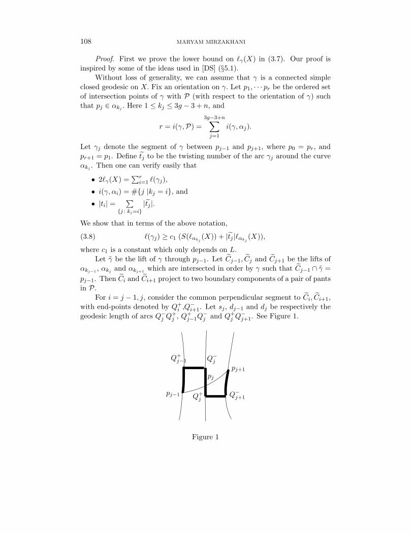
where c1 is a constant which only depends on L.Let γ be the lift of γ through pj−1. Let Cj−1, Cj and Cj+1 be the lifts of

αkj−1 , αkjand αkj+1 which are intersected in order by γ such that Cj−1 ∩ γ =

pj−1. Then Ci and Ci+1 project to two boundary components of a pair of pantsin P.

For i = j − 1, j, consider the common perpendicular segment to Ci, Ci+1,with end-points denoted by Q+

i ,Q−i+1. Let sj , dj−1 and dj be respectively the

geodesic length of arcs Q−j Q+

j , Q+j−1Q

−j and Q+

j Q−j+1. See Figure 1.

Q+j−1 Q−

j

pj

pj+1

pj−1 Q+j

Q−j+1

Figure 1


Then we have:

• dj ≥ S(�αkj), and

• the shift sj is given by sj = |tj �αkj+ ταkj

+ ej |, where |ej | < �αkj. Since

|ταkj| ≤ �αkj

, we get sj ≥ (|tj | − 2) �αkj.

Here both ej and tj are independent of the geometry of X. They only dependon the topology of γ relative to the pants decomposition P. See §5.1 in [DS]for more details.

As a result we have

dj + sj ≥ S(�αkj) + (|tj | − 2) �αkj

.(3.9)

Since P is L−bounded, �αi(X) ≤ L, and there exists a constant DL > 0

such that dj ≥ DL. Now equation (3.8) follows from the next two basic obser-vations:

(1) Let p1 and p2 be two points of distance x and z to a geodesic line.Consider the geodesic quadrangle p1q1q2p2 such that d(q1, q2)=y, d(p1, q1)=x,

and d(q2, p2) = z. If y ≥ D(L), then

d = d(p1, p2) ≥ c(L)(x + y + z),(3.10)

where c(L) is a constant depending only on L. To prove (3.10), note that bybasic hyperbolic trigonometry,

cosh(d) = cosh(x) cosh(z) cosh(y) − sinh(x) sinh(z).

Here x and z are oriented lengths; if p1 and p2 lie on opposite sides of q1q2,then x and z have opposite signs. See §2.3.2 of [Bus]. This formula impliesthat cosh(d) ≥ cosh(x) cosh(z)(cosh(y)−1). Hence there exists K = K(L) > 0such that

d ≥ x + y + z − K(L);(3.11)

see Lemma 5.1 of [DS]. Since d ≥ D(L), it is easy to see that

d ≥ min{12,

D(L)2K(L)

}(x + y + z).

(2) Note that for 0 ≤ x ≤ L, S(x)/x is bounded from below. Hence, by(3.9) there exists a constant c2 such that

dj + sj ≥ c2(L) (S(�αkj) + |tj | �αkj

).(3.12)

Therefore, by (3.10) for geodesic quadrangles pj−1 Q+j−1 Q−

j pj andpj Q+

j Q−j+1 pj+1 we have

�(γj) ≥ c(L)(dj + sj).(3.13)


Now equation (3.8) follows from (3.12) and (3.13). By adding the inequality(3.8) for 1 ≤ j ≤ r, we get

�γ(X) =12

r∑j=1

�(γj) ≥ C(L)LP(X, γ).

Let d(α, β) denote the length of the shortest geodesic path joining two bound-aries α and β of a pair of pants in the pants decomposition P. To obtain theupper bound on �γ(X), it is enough to note that d(α, β) ≤ c3 (S(�α(X)) +S(�β(X))), where the constant c3 depends only on L.

Upper and lower bounds for B(X). Next, we find upper and lower boundsfor the function B(X) in terms of the lengths of short geodesics on X. DefineR : R+ → R+ by

R(x) =1

x | log(x)| .

Proposition 3.6. For any X ∈ Tg,n, sufficiently small ε > 0 and 1 ≤ L,

C1 ·∏

γ : �γ(X)≤ε

R(�γ(X)) ≤ B(X),(3.14)

andbX(L)

L6g−6+2n≤ C2 ·

∏γ : �γ(X)≤ε

1�γ(X)

,(3.15)

where C1, C2 > 0 are constants depending only on g, n and ε.

Sketch of the proof. Take ε small enough such that no two closed geodesicsof length ≤ ε on a hyperbolic surface meet. For X ∈ Tg,n, let α1, . . . , αs bethe set of all simple closed geodesics of length ≤ ε on X and

PX = {α1, . . . , αs, . . . , αk}be a maximal set of disjoint simple closed geodesics such that �αi

(X) ≤ Lg,n,where k = 3g − 3 + n, and Lg,n is the Bers’ constant for Sg,n (see [Bus]). Wecan assume that PX is Lg,n−bounded on X.

Given x, y, L > 0, consider the set Ax,y(L) defined by

Ax,y(L) = {(m, n) | mx + ny ≤ L} ⊂ Z+ × Z+.

Then for L > 6 max{x, y}112

(L2

x · y

)≤ |Ax,y(L)|.(3.16)

Also, for L > 1

|Ax,y(L)| ≤ 3(

L2

x · y +L

min{x, y} + 1)

≤ 3L2(1 +1

x · y +1

min{x, y}).(3.17)


Now we can estimate bX(L), the number of integral multi-curves of length≤ L on X, by applying (3.7). We use the combinatorial length of multi-curvegeodesics with respect to the pants decomposition PX instead of their geodesiclength on X. By setting xi = S(�αi

(X)), yi = �αi(X), Theorem 3.4 implies

that

1c

k∏i=1

Axi,yi(L

k) ≤ bX(L) ≤ c

k∏i=1

Axi,yi(L),(3.18)

where c > 0 is a constant independent of X and L. Note that

{(mi, ti)3g−3+ni=1 | ∀i 1 ≤ i ≤ 3g − 3 + n, ti > 0, mi ∈ 2Z+} ⊂ Z(P).

On the other hand,S(x)/| log(x)| → 1

as x → 0. It is easy to check that:

• 1/c0 ≤ x · S(x) ≤ c0, for ε ≤ x ≤ Lg,n,

• c1 ≤ max{x, S(x)}, and

• min{x, S(x)} ≤ c2.

Here c0, c1 and c2 are constants which only depend on g, n and ε. Therefore,(3.14) follows from (3.16) and (3.18). Similarly, (3.15) follows from (3.17) and(3.18).

Properness and integrability of the function B. In this part we show thatthe upper bound in (3.15) is an integrable proper function.

Proof of Theorem 3.3. Note that inf{�γ}γ → 0 as X → ∞ in Mg,n. Also,

R(ε) → ∞as ε → 0. So equation (3.14) implies the function B is proper.

Next we prove that the function F : Mg,n → R defined by

F (X) =∏

γ : �γ(X)≤ε

1�γ(X)

,(3.19)

is integrable with respect to the Weil-Petersson volume form on Mg,n. LetMk,ε

g,n ⊂ Mg,n be the subset consisting of surfaces with k simple closed geodesicsof length ≤ ε. Note that using the Fenchel-Nielson coordinates, the set Mk,ε

g,n

can be covered by finitely many open sets of the form

π({(xi, yi)3g−3+n1 | 0 ≤ x1, . . . xk ≤ ε, xi ≤ Lg,n, 0 ≤ yi ≤ xi}).

See Section 2. By Theorem 2.1, it is enough to note that for

Vε,k = {(xi, yi)k1 | 0 ≤ x1, . . . xk ≤ ε, 0 ≤ yi ≤ xi}


β3

β1

β2

α

β4

β3

α1

α2 β4

β1

β2

Figure 2. Cutting a surface along a multi-curve

we have ∫Vε,k

1x1 · · ·xk

dx1 · · · dxk · dy1 · · · dyk < ∞.

Define fL : Mg,n → R+ by

fL(X) =bX(L)

L6g−g+2n.

By Proposition 3.6, the sequence {fL}L≥1 satisfies the hypothesis of Lebesgue’sdominated convergence theorem. In fact, for every integral multi-curve γ onSg,n, we have

sX(L, γ)L6g−6+2n

≤ fL(X) ≤ C2 · F (X),(3.20)

where the function F , defined by (3.19), is integrable over Mg,n.

4. Integration over the moduli space of hyperbolic surfaces

In this section, we recall the results obtained in [Mirz2] and [Mirz3] forintegrating certain geometric functions over the moduli space of hyperbolicsurfaces.

Symmetry group of a simple closed curve. For any set A of homotopyclasses of simple closed curves on Sg,n, define Stab(A) by

Stab(A) = {g ∈ Modg,n | g · A = A} ⊂ Modg,n .

Let γ =k∑

i=1aiγi, be a multi-curve on Sg,n. Define the symmetry group of γ,

Sym(γ), bySym(γ) = Stab(γ)/ ∩k

i=1 Stab(γi).

Note that for any connected simple closed curve α, |Sym(α)| = 1.


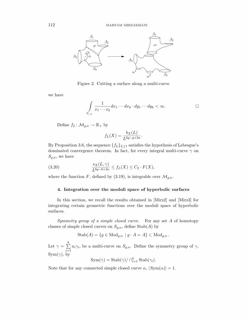
Splitting along a simple closed curve. Consider the surface Sg,n\Uγ , whereUγ is an open set homeomorphic to

⋃k1((0, 1) × γi). We denote this surface

by Sg,n(γ), which is a (possibly disconnected) surface with n + 2k boundarycomponents and s = s(γ) connected components. Each connected componentγi of γ, gives rise to two boundary components, γ1

i and γ2i on Sg,n(γ). Namely,

∂(Sg,n(γ)) = {β1, . . . , βn} ∪ {γ11 , γ2

1 , . . . , γ1k , γ2

k}.Now for Γ = (γ1, . . . , γk), and x = (x1, . . . , xk) ∈ Rk

+, let

T (Sg,n(γ), �Γ = x)

be the Teichmuller space of hyperbolic Riemann surfaces homeomorphic toSg,n(γ) such that �γi

= xi and �βi= 0. The group G(Γ) = ∩k

i=1 Stab(γi)naturally acts on T (Sg,n(γ), �Γ = x). Now, define

Mg,n(Γ,x) = T (Sg,n(γ), �Γ = x)/G(Γ).

Let Stab0(α) ⊂ Stab(α) denote the subgroup consisting of elements whichpreserve the orientation of α. Then any g ∈ ∩k

i=1 Stab0(γi) can be thought ofas an element in Mod(Sg,n(γ)). Hence for (g, n) �= (1, 1), M(Sg,n(γ), �Γ = x)is a finite cover of Mg,n(Γ,x) of order

N(γ) =

∣∣∣∣∣k⋂

i=1

Stab(γi)/k⋂

i=1

Stab0(γi)

∣∣∣∣∣ .

Therefore,

Volwp(Mg,n(Γ,x)) =1

N(γ)

s∏i=1

Vgi,ni(�Ai

),(4.1)

where

Sg,n(γ) =s⋃

i=1

Si ,

Si∼= Sgi,ni

, and Ai = ∂Si.

There is an exceptional case which arises when g = n = 1. In thiscase, every X ∈ M1,1 has a symmetry of order 2, τ ∈ Stab(γ). As a result,Vol(M1,1(Γ, x)) = 1.

Example. Let α be a connected nonseparating simple closed curve α onSg,n. Then there exists an element in Stab(α) which reverses the orientationof α, and hence N(α) = 2.

Simple closed curves on X ∈ Mg,n. Let [γ] denote the homotopy class ofa simple closed curve γ on Sg,n. Although there is no canonical simple closedgeodesic on X ∈ Mg,n corresponding to [γ], the set

Oγ = {[α]| α ∈ Mod ·γ},


of homotopy classes of simple closed curves in the Modg,n-orbit of γ on X, isdetermined by γ. In other words, Oγ is the set of [φ(γ)] where φ : Sg,n → X isa marking of X.

Integration over the moduli space of hyperbolic surfaces. For a multi-curve

γ =k∑

i=1aiγi, we have

�γ(X) =k∑

i=1

ai�γi(X).

Given a continuous function f : R+ → R+,

fγ(X) =∑

[α]∈Mod ·[γ]

f(�α(X)),(4.2)

defines a function fγ : Mg,n → R+. Then we can calculate the integral of fγ

over Mg,n using the following result [Mirz2]:

Theorem 4.1. For any multi-curve γ =k∑

i=1aiγi, the integral of fγ over

Mg,n with respect to the Weil-Petersson volume form is given by∫Mg,n

fγ(X) dX =2−M(γ)

|Sym(γ)|

∫x∈Rk

+

f(|x|) Vg,n(Γ,x) x · dx,

where Γ = (γ1, . . . , γk), |x| =k∑

i=1ai xi, x · dx = x1 · · ·xk · dx1 ∧ · · · ∧ dxk,

M(γ) = |{i|γi separates off a one-handle from Sg,n}|,and

Vg,n(Γ,x) = Volwp(Mg,n(Γ,x)).

By Theorem 4.1, integrating fγ , even for a compact Riemann surface,reduces to the calculation of volumes of moduli spaces of bordered Riemannsurfaces.

Idea of the proof of Theorem 4.1. Here we briefly sketch the main idea ofhow to calculate the integral of fγ over Mg,n with respect to the Weil-Peterssonvolume form when γ is a connected simple closed curve. See [Mirz2] for moredetails.

First, consider the covering space of Mg,n

πγ : Mγg,n = {(X, α) | X ∈ Mg,n, and α ∈ Oγ is a geodesic on X } → Mg,n,

where πγ(X, α) = X. The hyperbolic length function descends to the function

� : Mγg,n → R+


defined by �(X, η) = �η(X). Therefore,∫Mg,n

fγ(X) dX =∫

Mγg,n

f ◦ �(Y ) dY.

On the other hand, the function f is constant on each level set of � and wehave ∫

Mγg,n

f ◦ �(Y ) dY =

∞∫0

f(t) Vol(�−1(t)) dt,

where the volume is taken with respect to the volume form induced on �−1(t).The decomposition of the surface along the simple closed curve γ gives rise

to a description of Mγg,n in terms of moduli spaces corresponding to simpler

surfaces. This observation leads to formulas for the integral of fγ in termsof the Weil-Petersson volumes of moduli spaces of bordered Riemann surfacesand the function f as follows.

As before, let Sg,n(γ) denote the surface obtained by cutting the surfaceSg,n along γ. Also, Tg,n(γ, �γ = t) denotes the Teichmuller space of Riemannsurfaces homeomorphic to Sg,n(γ) such that the lengths of the two boundarycomponents corresponding to γ are equal to t. We have a natural circle bundle

�−1(t) ⊂ Mγg,n⏐⏐�

Mg,n(γ, �γ = t) = Tg,n(γ, �γ = t)/ Stab(γ).

We consider the S1-action on the level set �−1(t) ⊂ Mγg,n induced by twisting

the surface along γ. The quotient space �−1(t)/S1 inherits a symplectic formfrom the Weil-Petersson symplectic form. On the other hand, Mg,n(γ, �γ = t)is equipped with the Weil-Petersson symplectic form. Also,

�−1(t)/S1 ∼= Mg,n(γ, �γ = t)

as symplectic manifolds. So we expect to have

Vol(�−1(t)) = t Vol(Mg,n(γ, �γ = t)).

But the situation is different when γ separates off a one-handle in which casethe length of the fiber of the S1-action at a point is in fact t/2 instead of t

[Mirz2]. Hence, for any connected simple closed curve γ on Sg,n,

∫Mg,n

fγ(X) dX = 2−M(γ)

∞∫0

f(t) t Vol(Mg,n(γ, �γ = t)) dt,(4.3)

where M(γ) = 1 if γ separates off a one-handle, and M(γ) = 0 otherwise.


The Weil-Petersson volumes of the moduli spaces of hyperbolic surfaces.In [Mirz2], by using an identity for the lengths of simple closed geodesics onhyperbolic surfaces and using Theorem 4.1, we obtain a recursive method forcalculating volume polynomials.

Theorem 4.2. The volume Vg,n(b1, . . . , bn) = Volwp(Mg,n(b)) is a poly-nomial in b2

1, . . . , b2n; that is,

Vg,n(b) =∑

α

|α|≤3g−3+n

Cα · b 2α,

where Cα > 0 lies in π6g−6+2n−|2 α| · Q.

Theorem 4.3. The coefficient Cα in Theorem 4.2 is given by

Cα =1

2|α| |α|! (3g − 3 + n − |α|)!

∫Mg,n

ψα11 · · ·ψαn

n · ω3g−3+n−|α|,(4.4)

where ψi is the first Chern class of the ith tautological line bundle, ω is theWeil-Petersson symplectic form, α! =

∏ni=1 αi!, and |α| =

∑ni=1 αi.

See [Mirz2] and [Mirz3] for more details.

Examples. One can use the recursive formula obtained in [Mirz2], or othersimilar recursive formulas to calculate the coefficients of the volume polynomi-als.

(1) By [Mirz2],

V1,1(b) =124

(b2 + 4π2) ,(4.5)

V1,2(b1, b2) =1

192(4π2 + b2

1 + b22)(12π2 + b2

1 + b22).(4.6)

(2) In general, for g = 0, ∫M0,n

ψα11 · · ·ψαn

n =(

n − 3α1 . . . αn

).

(3) For n = 1 and g > 1, we have [FP], [IZ]:∫Mg,1

ψ6g−41 =

124gg!

.


Therefore, by Theorem 4.3 the leading coefficient of the polynomialVg,1(L) is equal to

L6g−4

24g g! (3g − 2)!23g−2.(4.7)

For more on calculating intersection pairings over Mg,n see [ArC].

5. Counting curves and Weil-Petersson volumes

In this section we establish a relationship between sX(L, γ) and theWeil-Petersson volume of moduli spaces of bordered Riemann surfaces. Weuse this relationship to calculate bg,n in terms of the leading coefficients ofvolume polynomials.

Let P (L, γ) be the integral of sX(L, γ) over Mg,n, given by

P (L, γ) =∫

Mg,n

sX(L, γ) dX.

Now by using Theorem 4.1 for f = χ([0, L]), we obtain the following result:

Proposition 5.1. For any multi-curve γ =k∑

i=1ai γi, the integral of

sX(L, γ) is given by

P (L, γ) =2−M(γ)

|Sym(γ)|

L∫0

∫k∑

i=1ai·xi=T

Vg,n(Γ,x) x dx dT,(5.1)

where x = (x1, . . . , xk), and Γ = (γ1, . . . , γk).

Note that even though Vg,n(Γ,x) depends on the choice of Γ = (γ1, . . . , γk),the right-hand side of (5.1) only depends on γ. Using Theorem 4.2, we get:

Corollary 5.2. For any multi-curve γ, P (L, γ) is a polynomial of degree6g−6+2n in L. If γ is a rational multi-curve, then c(γ), the leading coefficientof this polynomial, is a positive rational number.

Notation. Define c(γ) by

c(γ) = limL→∞

P (L, γ)L6g−6+2n

.(5.2)

By Corollary 5.2, c(γ) is the coefficient of L6g−6+2n in P (L, γ). Moreover, if γ

is a rational multi-curve, then by Theorem 4.2, c(γ) ∈ Q>0.


Let Γ = (γ1, . . . , γk). Recall that by Theorem 4.2,

Volwp(Mg,n(Γ,x))

is a polynomial of degree 6g−6+2n−2k in x1, . . . xk (see equation (4.1)). Let(2s1, . . . 2sk)Γ ∈ Q>0 denote the coefficient of x2s1

1 · · ·x2sk

k in this polynomial,and

bΓ(2s1, . . . , 2sk) = (2s1, . . . 2sk)Γ

∏ki=1(2si + 1)!

(6g − 6 + 2n)!.(5.3)

Also, as before

M(γ) = |{i|γi separates off a one-handle from Sg,n}|.

Let

Sg,n = {η| η is a union of simple closed curves on Sg,n}/ Modg,n .(5.4)

Note that |Sg,n| < ∞. An element η ∈ Sg,n can be written as η = η1 ∪ · · · ηk

where ηi’s are disjoint nonhomotopic, nonperipheral simple closed curves on

Sg,n. Then η =k∑

i=1ηi defines an integral multi-curve.

Calculation of c(γ) and bg,n. Now we can explicitly calculate the valueof the integral of the function B over Mg,n.

Theorem 5.3. In terms of the above notation, we have:

(1) The frequency c(γ) of a multi-curve γ =∑k

i=1 aiγi is equal to

c(γ) =2−M(γ)

|Sym(γ)| ×∑

s

|s|=3g−3+n−k

bΓ(2s1, . . . 2sk)a2s1+2

1 · · · a2sk+2k

.(5.5)

Here Γ = (γ1, . . . , γk), s = (s1, . . . , sk) ∈ Z+, and |s| =∑k

i=1 si.

(2) We have

bg,n =∑

η∈Sg,n

Bη,

where for η =⋃k

i=1 ηi,

Bη =2−M(η)

|Sym(η)| ×∑

|s|=3g−3+n−k

bη(2s1, . . . 2sk)k∏

i=1

ζ(2si + 2),

and η = (η1, . . . , ηk).


Proof. Part 1. To prove equation (5.5), note that given a1, · · · , ak ∈ R+,

and s1, · · · , sk ∈ Z+, we have∫a1x1+···+akxk=T

x2s1+11 · · ·x2sk+1

k dx1 · · · dxk

=(2s1 + 1)! · · · (2sk + 1)! · T 2|s|+2k−1

a2s1+21 · · · a2sk+2

k · (2|s| + 2k − 1)!.

Now the result follows from Theorem 4.2, (5.3), and Proposition 5.1.

Part 2. As a result of Proposition 3.1,

bg,n =∫

Mg,n

B(X)dX =∫

Mg,n

limL→∞

bX(L)L6g−6+2n

dX.

On the other hand, for any X ∈ Tg,n,

bX(L) =∑

η∈Sg,n

sX(L, η),

where for η = η1 ∪ . . . ∪ ηk ∈ Sg,n

sX(L, η) =∑

γ=∑

aiηi∈MLg,n(Z)

sX(L, γ).

Given η = (η1, . . . , ηk), and a ∈ Nk, let a · η =k∑

i=1ai · ηi ∈ MLg,n(Z). It is

easy to check that Sym(a · η) ⊂ Sym(η), and

|{a1 ∈ Nk | ∃ g ∈ Modg,n a1 · η = g (a · η)}| =|Sym(η)|

|Sym(a · η)| .

Therefore, we have

sX(L, η) =∑a∈Nk

|Sym(a · η)||Sym(η)| sX(L,a · η).

Hence,

bg,n =∑

η∈Sg,n

∫Mg,n

limL→∞

sX(L, η)L6g−6+2n

dX.

Now (3.20) allows us to use Lebesgue’s dominated convergence theorem. As aresult, we get∫

Mg,n

limL→∞

sX(L, η)L6g−6+2n

dX =∑a∈Nk

|Sym(a · η)||Sym(η)| lim

L→∞P (L,a · η)L6g−6+2n

=∑a∈Nk

|Sym(a · η)||Sym(η)| c(a · η).

Now the result follows from (5.5). See [Mirz1] for more details.


Note that by Theorem 4.2, for |s| = 3g − 3 − k, bη(2s1, . . . , 2sk) ∈ Q>0.On the other hand, ζ(2i) ∈ π2i · Q. Hence we get:

Corollary 5.4. For any g, n, with 2g − 2 + n > 0, bg,n is a rationalmultiple of π6g−6+2n.

In the simplest case when g = n = 1, |S1,1| = 1, and

b1,1 = ζ(2) =π2

6.

6. Counting different types of simple closed curves

In this section we use the ergodicity of the action of the mapping classgroup on the space of measured laminations to obtain the following results:

Theorem 6.1. For any rational multi-curve γ and X ∈ Tg,n,

sX(L, γ) ∼ B(X)bg,n

c(γ) L6g−6+2n,

as L → ∞.

Note that bg,n and c(γ) (defined by equations (3.4) and (5.2)) are bothconstants independent of X and L; see Theorem 5.3. Therefore, we get:

Corollary 6.2. For any X ∈ Tg,n, as L → ∞sX(L, γ1)sX(L, γ2)

→ c(γ1)c(γ2)

.

Since there are only finitely many isotopy classes of simple closed curveson Sg,n up to the action of the mapping class group, the following result isimmediate:

Corollary 6.3. The number of simple closed geodesics of length ≤ L onX ∈ Mg,n has the asymptotic behavior

sX(L) ∼ n(X)L6g−6+2n

as L → ∞, where n : Mg,n → R+ is proper and continuous.

Discrete measures on MLg,n. Any γ ∈ MLg,n(Z), defines a sequence ofdiscrete measures on MLg,n, {μT,γ}, such that for any open set U ⊂ MLg,n

μT,γ(U) =#(T · U ∩ Modg,n ·γ)

T 6g−6+2n.

There is a close relation between the asymptotic behavior of this sequence ofmeasures and counting different types of simple closed geodesics. First, weprove the following result on the asymptotic behavior of μT,γ as T → ∞:


Theorem 6.4. For any rational multi-curve γ, as T → ∞

μT,γw∗−→ c(γ)

bg,n· μTh,(6.1)

where μTh is the Thurston volume form on MLg,n.

Remarks. 1. Let Y be a closed orientable surface of genus g with boundednegative curvature. Then each homotopy class of closed curves contains aunique closed geodesic. Consider the space ML(Y ) of measured geodesic lam-inations on Y and let �γ(Y ) be the geodesic length of γ on Y . The length func-tion extends to a continuous function on ML(Y ). Moreover, ML(Y ) ∼= MLg.Since Theorem 6.4 is independent of the Riemannian metric on the surface,both Theorem 6.1 and Corollary 6.2 hold for Y .

2. Using the same method, one can check that the results of Theorem 6.1and Corollary 6.2 also hold for any hyperbolic surface X ∈ Mg,n(L1, . . . , Ln)with geodesic boundary components.

Proof of Theorem 6.4. It is enough to prove the result for integral multi-curves. The argument has three main steps:

Step 1. Given X0 ∈ Tg,n, by Proposition 3.6, and (3.20) we have

μT,γ(L · BX0) =sX0(L T, γ)T 6g−6+2n

≤ C(X0, L),

where C(X0, L) is a constant depending only on X0 and L. In particular it isindependent of T . On the other hand, given a compact subset K ⊂ MLg,n,there exists L such that K ⊂ L · BX0 . As a result, we have

lim supT→∞

μT,γ(K) < ∞.

Therefore, any subsequence of {μT,γ} contains a weakly-convergent subse-quence.

Step 2. We show that any weak limit of the sequence {μT,γ} is a multipleof the measure μTh. Assume that

μTi,γ → νJ(6.2)

as Ti ∈ J → ∞. We show that νJ belongs to the Lebesgue measure class; thatis for any V ⊂ MLg,n with μTh(V ) = 0, we have νJ(V ) = 0. Let U ⊂ MLg,n

be a convex open set in a train track chart. Using Proposition 3.1, we have:

νJ(U) ≤ lim infi→∞

μTi,γ(U) ≤ limi→∞

b(Ti, U)

T 6g−6+2ni

= μTh(U).(6.3)

Since we can approximate V with open subsets of MLg,n satisfying (6.3), themeasure νJ belongs to the Lebesgue measure class. Then the ergodicity of the


action of the mapping class group on MLg,n (Theorem 2.2) implies that

νJ = kJ μTh.

Step 3. Finally, we show vJ = k · μTh, where k is independent of thesubsequence J . Note that for any X ∈ Tg,n, sX(T, γ) = μT,γ(BX). Equation(6.2) implies:

sX(Ti, γ)

T 6g−6+2ni

→ kJ · B(X)(6.4)

as i → ∞. Now we integrate both sides of (6.4) over Mg,n. By using (3.20),Corollary 5.2, and (5.2), we get

kJ · bg,n = kJ ·∫

Mg,n

B(X) dX =∫

Mg,n

limi→∞

sX(Ti, γ)

T 6g−6+2ni

dX

= limi→∞

∫Mg,n

sX(Ti, γ)

T 6g−6+2ni

dX = limi→∞

P (Ti, γ)

T 6g−6+2ni

= c(γ).

On the other hand, by Theorem 3.3, bg,n < ∞. Therefore,

kJ =c(γ)bg,n

is independent of J , and hence

μT,γ → c(γ)bg,n

· μTh.

Proof of Theorem 6.1. Since ∂BX has measure zero, equation (6.1)implies that

μT,γ(BX) → c(γ)bg,n

· μTh(BX).

Now the result is immediate since

μT,γ(BX) =#(L · BX ∩ Modg,n ·γ)

L6g−6+2n=

sX(L, γ)L6g−6+2n

.

Examples. Here we explicitly calculate the frequencies of different typesof simple closed curves in some simple cases.

(1) First, we consider the case of g = 2. Then by equation (4.6), for anynonseparating simple closed curve α1

Vol(M(S2(α1), �α1 = x)) = V1,2(x, x) =148

(2π2 + x2)(6π2 + x2).


Since N(α1) = 2 and M(α1) = 0, the leading coefficient of P (L, α1) isequal to 1

2×48×6 . Equation (5.5) implies that

c(α1) =1

2 × 48 × 6.

Similarly, by equation (4.5), for any separating simple closed curve α2,

Vol(M(S2(α2), �α2 = x)) = V1,1(x) × V1,1(x) = (x2

24+

π2

6)2.

In this case, M(α2) = 1, and N(α2) = 2. By equation (5.5)

c(α2) =1

24 × 24 × 6.

Hence, Corollary 6.2 implies that

limL→∞

sX(L, α1)sX(L, α2)

=c(α1)c(α2)

= 6.

Roughly speaking, on a surface of genus 2, a long, random connected,simple, closed geodesic is separating with probability 1

7 .

(2) Let βi be a connected simple closed curve on S0,n satisfying

S0,n(βi) ∼= S0,i+1 ∪ S0,n−i+1.

Then as in Section 4, the coefficient of L2n−41 in V0,n+1(L1, ..., Ln, Ln+1)

equals 12n−2(n−2)! . In this case, N(βi) = |Sym(βi)| = 1. Hence, by (5.5),

we havec(βi) =

12n−4(i − 2)! (n − i − 2)! (2n − 6)

.

Hence, given X ∈ T0,n

sX(L, βi)sX(L, βj)

→(n−4i−2

)(n−4j−2

)as L → ∞.

(3) Let γi be a separating connected simple closed curve on a surface of genusg that cuts the surface into two parts of genus i and g− i. For simplicity,we assume that g > 2i > 2. In this case, N(γi) = 1 and M(γi) = 0. Also,

Vol(M(Sg(γi), �γi= x)) = Vi,1(x) × Vg−i,1(x).

On the other hand, by (4.7) the leading term of the polynomial Vg,1(L)is equal to

L6g−4

(3g − 2)! g! 24g23g−2.


Now since |Sym(γi)| = 1, by (5.5) the frequency of a simple closed curveof type γi is equal to

c(γi) =1

23g−224g i!(g − i)! (3g − 2)!(3(g − i) − 2)!(6g − 6).

For X ∈ Tg, we have

limL→∞

sX(L, γi)bX(L)

=c(γi)bg

.

Princeton University, Princeton, NJ

E-mail address: [email protected]

References

[ArC] C. Arbarello and M. Cornalba, Combinatorial and algebro-geometric cohomologyclasses on the moduli spaces of curves, J. Algebraic Geom. 5 (1996), 705–749.

[BS1] J. S. Birman and C. Series, An algorithm for simple curves on surfaces, J. LondonMath. Soc. 29 (1984), 331–342.

[BS2] ———, Geodesics with bounded intersection number on surfaces are sparsely dis-tributed, Topology 24 (1985), 217–225.

[Bus] P. Buser, Geometry and Spectra of Compact Riemann Surfaces, Progr. in Math. 106,Birkhauser Boston, 1992.

[DS] R. Diaz and C. Series, Limit points of lines of minima in Thurston’s boundary ofTeichmuller space, Algebr. Geom. Topol. 3 (2003), 207–234.

[FP] C. Faber and R. Pandharipande, Hodge integrals and Gromov-Witten theory, Invent.math. 139 (2000), 173–199.

[FLP] A. Fathi, F. Laudenbach, and V. Poenaru, Travaux de Thurston sur les Surfaces,Asterisque 66–67, Soc. Math. France, Paris, 1979.

[Gol] W. Goldman, The symplectic nature of fundamental groups of surfaces, Adv. Math.54 (1984), 200–225.

[HP] J. L. Harer and R. C. Penner, Combinatorics of Train Tracks, Ann. of Math. Studies125, Princeton Univ. Press, Princeton, NJ, 1992.

[IZ] C. Itzykson and J. Zuber, Combinatorics of the modular group. II. The Kontsevichintegrals, Internat. J. Modern Phys. A 7 (1992), 5661–5705.

[Ker] S. Kerckhoff, Earthquakes are analytic, Comment. Math. Helv . 60 (1985), 17–30.

[Ma] G. A. Margulis, Applications of ergodic theory to the investigation of manifolds ofnegative curvature, Funct. Anal. Appl. 4 (1969), 335–336.

[Mas1] H. Masur, Interval exchange transformations and measured foliations, Ann. of Math.115 (1982), 169–200.

[Mas2] ———, Ergodic actions of the mapping class group, Proc. Amer. Math. Soc. 94(1985), 455–459.

[MR] G. McShane and I. Rivin, Simple curves on hyperbolic tori, C. R. Acad. Sci. ParisSer . I Math. 320 (1995), 1523–1528.


[Mirz1] M. Mirzakhani, Simple geodesics on hyperbolic surfaces and the volume of the modulispace of curves, Ph.D. thesis, Harvard University, 2004.

[Mirz2] ———, Simple geodesics and Weil-Petersson volumes of moduli spaces of borderedRiemann surfaces, Invent. Math. 167 (2007), 179–222.

[Mirz3] ———, Weil-Petersson volumes and intersection theory on the moduli space ofcurves, J. Amer. Math. Soc. 20 (2007), 1–23.

[Rs] M. Rees, An alternative approach to the ergodic theory of measured foliations onsurfaces, Ergodic Theory Dynamical Systems 1 (1981), 461–488.

[Ri] I. Rivin, Simple curves on surfaces, Geom. Dedicata 87 (2001), 345–360.

[Th] W. P. Thurston, Geometry and topology of three-manifolds, Lecture Notes, PrincetonUniversity, 1979.

[Wol] S. Wolpert, The Fenchel-Nielsen deformation, Ann. of Math. 115 (1982), 501–528.

[Z] D. Zagier, On the number of Markoff numbers below a given bound, Math. Comp.39 (1982), 709–723.

(Received April 11, 2004)

Date post:	03-May-2018
Category:	Documents
Upload:	ngodien
View:	215 times
Download:	1 times

Growth of the number of simple closed geodesics on...

Documents