Annals of Mathematics, 168 (2008), 859–914 Quasilinear and Hessian equations of Lane-Emden type By Nguyen Cong Phuc and Igor E. Verbitsky* Abstract The existence problem is solved, and global pointwise estimates of solu- tions are obtained for quasilinear and Hessian equations of Lane-Emden type, including the following two model problems: -Δ p u = u q + μ, F k [-u]= u q + μ, u ≥ 0, on R n , or on a bounded domain Ω ⊂ R n . Here Δ p is the p-Laplacian defined by Δ p u = div (∇u|∇u| p-2 ), and F k [u] is the k-Hessian defined as the sum of k × k principal minors of the Hessian matrix D 2 u (k =1, 2,...,n); μ is a nonnegative measurable function (or measure) on Ω. The solvability of these classes of equations in the renormalized (entropy) or viscosity sense has been an open problem even for good data μ ∈ L s (Ω), s> 1. Such results are deduced from our existence criteria with the sharp exponents s = n(q-p+1) pq for the first equation, and s = n(q-k) 2kq for the second one. Furthermore, a complete characterization of removable singularities is given. Our methods are based on systematic use of Wolff’s potentials, dyadic models, and nonlinear trace inequalities. We make use of recent advances in potential theory and PDE due to Kilpel¨ ainen and Mal´ y, Trudinger and Wang, and Labutin. This enables us to treat singular solutions, nonlocal operators, and distributed singularities, and develop the theory simultaneously for quasi- linear equations and equations of Monge-Amp` ere type. 1. Introduction We study a class of quasilinear and fully nonlinear equations and in- equalities with nonlinear source terms, which appear in such diverse areas as quasi-regular mappings, non-Newtonian fluids, reaction-diffusion problems, and stochastic control. In particular, the following two model equations are of *N. P. was supported in part by NSF Grants DMS-0070623 and DMS-0244515. I. V. was supported in part by NSF Grant DMS-0070623.
Transcript
Annals of Mathematics, 168 (2008), 859–914
Quasilinear and Hessian equationsof Lane-Emden type
By Nguyen Cong Phuc and Igor E. Verbitsky*
Abstract
The existence problem is solved, and global pointwise estimates of solu-tions are obtained for quasilinear and Hessian equations of Lane-Emden type,including the following two model problems:
−∆pu = uq + µ, Fk[−u] = uq + µ, u ≥ 0,
on Rn, or on a bounded domain Ω ⊂ Rn. Here ∆p is the p-Laplacian definedby ∆pu = div (∇u|∇u|p−2), and Fk[u] is the k-Hessian defined as the sum ofk × k principal minors of the Hessian matrix D2u (k = 1, 2, . . . , n); µ is anonnegative measurable function (or measure) on Ω.
The solvability of these classes of equations in the renormalized (entropy)or viscosity sense has been an open problem even for good data µ ∈ Ls(Ω),s > 1. Such results are deduced from our existence criteria with the sharpexponents s = n(q−p+1)
pq for the first equation, and s = n(q−k)2kq for the second
one. Furthermore, a complete characterization of removable singularities isgiven.
Our methods are based on systematic use of Wolff’s potentials, dyadicmodels, and nonlinear trace inequalities. We make use of recent advances inpotential theory and PDE due to Kilpelainen and Maly, Trudinger and Wang,and Labutin. This enables us to treat singular solutions, nonlocal operators,and distributed singularities, and develop the theory simultaneously for quasi-linear equations and equations of Monge-Ampere type.
1. Introduction
We study a class of quasilinear and fully nonlinear equations and in-equalities with nonlinear source terms, which appear in such diverse areasas quasi-regular mappings, non-Newtonian fluids, reaction-diffusion problems,and stochastic control. In particular, the following two model equations are of
*N. P. was supported in part by NSF Grants DMS-0070623 and DMS-0244515. I. V. wassupported in part by NSF Grant DMS-0070623.
860 NGUYEN CONG PHUC AND IGOR E. VERBITSKY
substantial interest:
(1.1) −∆pu = f(x, u), Fk[−u] = f(x, u),
on Rn, or on a bounded domain Ω ⊂ Rn, where f(x, u) is a nonnegative func-tion, convex and nondecreasing in u for u ≥ 0. Here ∆pu = div (∇u |∇u|p−2)is the p-Laplacian (p > 1), and Fk[u] is the k-Hessian (k = 1, 2, . . . , n) definedby
(1.2) Fk[u] =∑
1≤i1<···<ik≤nλi1 · · ·λik ,
where λ1, . . . , λn are the eigenvalues of the Hessian matrix D2u. In otherwords, Fk[u] is the sum of the k × k principal minors of D2u, which coincideswith the Laplacian F1[u] = ∆u if k = 1, and the Monge–Ampere operatorFn[u] = det (D2u) if k = n.
The form in which we write the second equation in (1.1) is chosen onlyfor the sake of convenience, in order to emphasize the profound analogy be-tween the quasilinear and Hessian equations. Obviously, it may be stated as(−1)k Fk[u] = f(x, u), u ≥ 0, or Fk[u] = f(x,−u), u ≤ 0.
The existence and regularity theory, local and global estimates of sub-and super-solutions, the Wiener criterion, and Harnack inequalities associatedwith the p-Laplacian, as well as more general quasilinear operators, can befound in [HKM], [IM], [KM2], [M1], [MZ], [S1], [S2], [SZ], [TW4] where manyfundamental results, and relations to other areas of analysis and geometry arepresented.
The theory of fully nonlinear equations of Monge-Ampere type whichinvolve the k-Hessian operator Fk[u] was originally developed by Caffarelli,Nirenberg and Spruck, Ivochkina, and Krylov in the classical setting. We re-fer to [CNS], [GT], [Gu], [Iv], [Kr], [Tru2], [TW1], [Ur] for these and furtherresults. Recent developments concerning the notion of the k-Hessian measure,weak continuity, and pointwise potential estimates due to Trudinger and Wang[TW2]–[TW4], and Labutin [L] are used extensively in this paper.
We are specifically interested in quasilinear and fully nonlinear equationsof Lane-Emden type:
(1.3) −∆pu = uq, and Fk[−u] = uq, u ≥ 0 in Ω,
where p > 1, q > 0, k = 1, 2, . . . , n, and the corresponding nonlinear inequali-ties:
(1.4) −∆pu ≥ uq, and Fk[−u] ≥ uq, u ≥ 0 in Ω.
The latter can be stated in the form of the inhomogeneous equations withmeasure data,
(1.5) −∆pu = uq + µ, Fk[−u] = uq + µ, u ≥ 0 in Ω,
where µ is a nonnegative Borel measure on Ω.
QUASILINEAR AND HESSIAN EQUATIONS 861
The difficulties arising in studies of such equations and inequalities withcompeting nonlinearities are well known. In particular, (1.3) may have singularsolutions [SZ]. The existence problem for (1.5) has been open ([BV2, Prob-lems 1 and 2]; see also [BV1], [BV3], [Gre]) even for the quasilinear equation−∆pu = uq + f with good data f ∈ Ls(Ω), s > 1. Here solutions are gener-ally understood in the renormalized (entropy) sense for quasilinear equations,and viscosity, or the k-convexity sense, for fully nonlinear equations of Hessiantype (see [BMMP], [DMOP], [JLM], [TW1]–[TW3], [Ur]). Precise definitionsof these classes of admissible solutions are given in Sections 3, 6, and 7 below.
In this paper, we present a unified approach to (1.3)–(1.5) which makes itpossible to attack a number of open problems. This is based on global point-wise estimates, nonlinear integral inequalities in Sobolev spaces of fractionalorder, and analysis of dyadic models, along with the Hessian measure andweak continuity results [TW2]–[TW4]. The latter are used to bridge the gapbetween the dyadic models and partial differential equations. Some of thesetechniques were developed in the linear case, in the framework of Schrodingeroperators and harmonic analysis [ChWW], [Fef], [KS], [NTV], [V1], [V2], andapplications to semilinear equations [KV], [VW], [V3].
Our goal is to establish necessary and sufficient conditions for the exis-tence of solutions to (1.5), sharp pointwise and integral estimates for solutionsto (1.4), and a complete characterization of removable singularities for (1.3).We are mostly concerned with admissible solutions to the corresponding equa-tions and inequalities. However, even for locally bounded solutions, as in [SZ],our results yield new pointwise and integral estimates, and Liouville-type the-orems.
In the “linear case” p = 2 and k = 1, problems (1.3)–(1.5) with nonlinearsources are associated with the names of Lane and Emden, as well as Fowler.Authoritative historical and bibliographical comments can be found in [SZ].An up-to-date survey of the vast literature on nonlinear elliptic equations withmeasure data is given in [Ver], including a thorough discussion of related workdue to D. Adams and Pierre [AP], Baras and Pierre [BP], Berestycki, Capuzzo-Dolcetta, and Nirenberg [BCDN], Brezis and Cabre [BC], Kalton and Verbitsky[KV].
It is worth mentioning that related equations with absorption,
(1.6) −∆u+ uq = µ, u ≥ 0 in Ω,
were studied in detail by Benilan and Brezis, Baras and Pierre, and Marcus andVeron analytically for 1 < q <∞, and by Le Gall, and Dynkin and Kuznetsovusing probabilistic methods when 1 < q ≤ 2 (see [D], [Ver]). For a generalclass of semilinear equations
(1.7) −∆u+ g(u) = µ, u ≥ 0 in Ω,
862 NGUYEN CONG PHUC AND IGOR E. VERBITSKY
where g belongs to the class of continuous nondecreasing functions such thatg(0) = 0, sharp existence results have been obtained quite recently by Brezis,Marcus, and Ponce [BMP]. It is well known that equations with absorptiongenerally require “softer” methods of analysis, and the conditions on µ whichensure the existence of solutions are less stringent than in the case of equationswith source terms.
Quasilinear problems of Lane-Emden type (1.3)–(1.5) have been studiedextensively over the past 15 years. Universal estimates for solutions, Liouville-type theorems, and analysis of removable singularities are due to Bidaut-Veron,Mitidieri and Pohozaev [BV1]–[BV3], [BVP], [MP], and Serrin and Zou [SZ].(See also [BiD], [Gre], [Ver], and the literature cited there.) The profounddifficulties in this theory are highlighted by the presence of the two criticalexponents,
(1.8) q∗ = n(p−1)n−p , q∗ = n(p−1)+p
n−p ,
where 1 < p < n. As was shown in [BVP], [MP], and [SZ], the quasilinearinequality (1.5) does not have nontrivial weak solutions on Rn, or exteriordomains, if q ≤ q∗. For q > q∗ , there exist u ∈ W 1, p
loc ∩ L∞loc which obeys
(1.4), as well as singular solutions to (1.3) on Rn. However, for the existenceof nontrivial solutions u ∈ W 1,p
loc ∩ L∞loc to (1.3) on Rn, it is necessary and
sufficient that q ≥ q∗ [SZ]. In the “linear case” p = 2, this is classical ([GS],[BP], [BCDN]).
The following local estimates of solutions to quasilinear inequalities areused extensively in the studies mentioned above (see, e.g., [SZ, Lemma 2.4]).Let BR denote a ball of radius R such that B2R ⊂ Ω. Then, for every solutionu ∈W 1,p
loc ∩ L∞loc to the inequality −∆pu ≥ uq in Ω,∫
BR
uγ dx ≤ C Rn−γp
q−p+1 , 0 < γ < q,(1.9) ∫BR
|∇u|γpq+1 dx ≤ C Rn−
γpq−p+1 , 0 < γ < q,(1.10)
where the constants C in (1.9) and (1.10) depend only on p, q, n, γ. Note that(1.9) holds even for γ = q (cf. [MP]), while (1.10) generally fails in this case.In what follows, we will substantially strengthen (1.9) in the end-point caseγ = q, and obtain global pointwise estimates of solutions.
In [PV], we proved that all compact sets E ⊂ Ω of zero Hausdorff measure,
Hn− pq
q−p+1 (E) = 0, are removable singularities for the equation −∆pu = uq,q > q∗. Earlier results of this kind, under a stronger restriction cap
1,pq
q−p+1 +ε(E)
= 0 for some ε > 0, are due to Bidaut-Veron [BV3]. Here cap1, s(·) is the ca-pacity associated with the Sobolev space W 1, s.
In fact, much more is true. We will show below that a compact set E ⊂ Ωis a removable singularity for −∆pu = uq if and only if it has zero fractional
QUASILINEAR AND HESSIAN EQUATIONS 863
capacity: capp,
qq−p+1
(E) = 0. Here capα, s stands for the Bessel capacity
associated with the Sobolev space Wα, s which is defined in Section 2. Weobserve that the usual p-capacity cap1, p used in the studies of the p-Laplacian[HKM], [KM2] plays a secondary role in the theory of equations of Lane-Emdentype. Relations between these and other capacities used in nonlinear PDEtheory are discussed in [AH], [M2], and [V4].
Our characterization of removable singularities is based on the solution ofthe existence problem for the equation
(1.11) −∆pu = uq + µ, u ≥ 0,
with nonnegative measure µ obtained in Section 6. Main existence theoremsfor quasilinear equations are stated below (Theorems 2.3 and 2.10). Here weonly mention the following corollary in the case Ω = Rn: If (1.11) has anadmissible solution u, then
(1.12)∫BR
dµ ≤ C Rn−pq
q−p+1 ,
for every ball BR in Rn, where C = C(p, q, n), provided 1 < p < n and q > q∗;if p ≥ n or q ≤ q∗, then µ = 0.
Conversely, suppose that 1 < p < n, q > q∗, and dµ = f dx, f ≥ 0, where
(1.13)∫BR
f1+ε dx ≤ C Rn−(1+ε)pqq−p+1 ,
for some ε > 0. Then there exists a constant C0(p, q, n) such that (1.11) hasan admissible solution on Rn if C ≤ C0(p, q, n).
The preceding inequality is an analogue of the classical Fefferman-Phongcondition [Fef] which appeared in applications to Schrodinger operators. Inparticular, (1.13) holds if f ∈ L
n(q−p+1)pq
,∞(Rn). Here Ls,∞ stands for the weakLs space. This sufficiency result, which to the best of our knowledge is neweven in the Ls scale, provides a comprehensive solution to Problem 1 in [BV2].Notice that the exponent s = n(q−p+1)
pq is sharp. Broader classes of measuresµ (possibly singular with respect to Lebesgue measure) which guarantee theexistence of admissible solutions to (1.11) will be discussed in the sequel.
A substantial part of our work is concerned with integral inequalities fornonlinear potential operators, which are at the heart of our approach. Weemploy the notion of Wolff’s potential introduced originally in [HW] in relationto the spectral synthesis problem for Sobolev spaces. For a nonnegative Borelmeasure µ on Rn, s ∈ (1, +∞), and α > 0, the Wolff’s potential Wα, s µ isdefined by
(1.14) Wα, s µ(x) =∫ ∞
0
[µ(Bt(x))tn−αs
] 1s−1 dt
t, x ∈ Rn.
864 NGUYEN CONG PHUC AND IGOR E. VERBITSKY
We write Wα, s f in place of Wα, s µ if dµ = fdx, where f ∈ L1loc(Rn), f ≥ 0.
When dealing with equations in a bounded domain Ω ⊂ Rn, a truncated versionis useful:
(1.15) Wrα, s µ(x) =
∫ r
0
[µ(Bt(x))tn−αs
] 1s−1 dt
t, x ∈ Ω,
where 0 < r ≤ 2diam(Ω). In many instances, it is more convenient to workwith the dyadic version, also introduced in [HW]:
(1.16) Wα, s µ(x) =∑Q∈D
[ µ(Q)`(Q)n−αs
] 1s−1
χQ(x), x ∈ Rn,
where D = Q is the collection of the dyadic cubes Q = 2i(k + [0, 1)n),i ∈ Z, k ∈ Zn, and `(Q) is the side length of Q.
An indispensable source on nonlinear potential theory is provided by [AH],where the fundamental Wolff’s inequality and its applications are discussed.Very recently, an analogue of Wolff’s inequality for general dyadic and radiallydecreasing kernels was obtained in [COV]; some of the tools developed thereare employed below.
The dyadic Wolff’s potentials appear in the following discrete model of(1.5) studied in Section 3:
(1.17) u =Wα, s uq + f, u ≥ 0.
As it turns out, this nonlinear integral equation with f =Wα, s µ is intimatelyconnected to the quasilinear differential equation (1.11) in the case α = 1,s = p, and to its k-Hessian counterpart in the case α = 2k
k+1 , s = k+1. Similardiscrete models are used extensively in harmonic analysis and function spaces(see, e.g., [NTV], [St2], [V1]).
The profound role of Wolff’s potentials in the theory of quasilinear equa-tions was discovered by Kilpelainen and Maly [KM2]. They established lo-cal pointwise estimates for nonnegative p-superharmonic functions in terms ofWolff’s potentials of the associated p-Laplacian measure µ. More precisely, ifu ≥ 0 is a p-superharmonic function in B3r(x) such that −∆pu = µ, then
(1.18) C1 Wr1, p µ(x) ≤ u(x) ≤ C2 inf
B(x,r)u+ C3 W2r
1, p µ(x),
where C1, C2 and C3 are positive constants which depend only on n and p.In [TW1], [TW2], Trudinger and Wang introduced the notion of the Hes-
sian measure µ[u] associated with Fk[u] for a k-convex function u. Very re-cently, Labutin [L] proved local pointwise estimates for Hessian equations anal-ogous to (1.18), where Wolff’s potential Wr
2kk+1
, k+1µ is used in place of Wr
1, p µ.
In what follows, we will need global pointwise estimates of this type. Inthe case of a k-convex solution to the equation Fk[u] = µ on Rn such that
QUASILINEAR AND HESSIAN EQUATIONS 865
infx∈Rn (−u(x)) = 0, one has
(1.19) C1 W 2kk+1
, k+1 µ(x) ≤ −u(x) ≤ C2 W 2kk+1
, k+1 µ(x),
where C1 and C2 are positive constants which depend only on n and k. Analo-gous global estimates are obtained below for admissible solutions of the Dirich-let problem for −∆pu = µ and Fk[−u] = µ in a bounded domain Ω ⊂ Rn (see§2).
In the special case Ω = Rn, our criterion for the solvability of (1.11) canbe stated in the form of the pointwise condition involving Wolff’s potentials:
(1.20) W1, p (W1, p µ )q (x) ≤ CW1, p µ(x) < +∞ a.e.,
which is necessary with C = C1(p, q, n), and sufficient with another constantC = C2(p, q, n). Moreover, in the latter case there exists an admissible solutionu to (1.11) such that
(1.21) c1 W1, p µ(x) ≤ u(x) ≤ c2 W1, p µ(x), x ∈ Rn,
where c1 and c2 are positive constants which depend only on p, q, n, provided1 < p < n and q > q∗; if p ≥ n or q ≤ q∗ then u = 0 and µ = 0.
The iterated Wolff’s potential condition (1.20) is crucial in our approach.As we will demonstrate in Section 5, it turns out to be equivalent to thefractional Riesz capacity condition
(1.22) µ(E) ≤ C Capp, q
q−p+1(E),
where C does not depend on a compact set E ⊂ Rn. Such classes of measuresµ were introduced by V. Maz’ya in the early 60-s in the framework of linearproblems.
It follows that every admissible solution u to (1.11) on Rn obeys the in-equality
(1.23)∫Euq dx ≤ C Capp, q
q−p+1(E),
for all compact sets E ⊂ Rn. We also prove an analogous estimate in a boundeddomain Ω (Section 6). Obviously, this yields (1.9) in the end-point case γ = q.In the critical case q = q∗, we obtain an improved estimate (see Corollary 6.13):
(1.24)∫Br
uq∗ dx ≤ C(log(2R
r )) 1−pq−p+1 ,
for every ball Br of radius r such that Br ⊂ BR, and B2R ⊂ Ω. CertainCarleson measure inequalities are employed in the proof of (1.24). We observethat these estimates yield Liouville-type theorems for all admissible solutionsto (1.11) on Rn, or in exterior domains, provided q ≤ q∗ (cf. [BVP], [SZ]).
866 NGUYEN CONG PHUC AND IGOR E. VERBITSKY
Analogous results will be established in Section 7 for equations of Lane-Emden type involving the k-Hessian operator Fk[u]. We will prove that thereexists a constant C1(k, q, n) such that, if
(1.25) W 2kk+1
, k+1(W 2kk+1
, k+1µ)q(x) ≤ CW 2kk+1
, k+1µ(x) < +∞ a.e.,
where 0 ≤ C ≤ C1(k, q, n), then the equation
(1.26) Fk[−u] = uq + µ, u ≥ 0,
has a solution u so that −u is k-convex on Rn, and
(1.27) c1 W 2kk+1
, k+1 µ(x) ≤ u(x) ≤ c2 W 2kk+1
, k+1 µ(x), x ∈ Rn,
where c1, c2 are positive constants which depend only on k, q, n, for 1 ≤ k < n2 .
Conversely, (1.25) with C = C2(k, q, n) is necessary in order that (1.26) has asolution u such that −u is k-convex on Rn provided 1 ≤ k < n
2 and q > q∗ =nkn−2k ; if k ≥ n
2 or q ≤ q∗ then u = 0 and µ = 0.
In particular, (1.25) holds if dµ=f dx, where f≥0 and f ∈Ln(q−k)
2kq,∞(Rn);
the exponent n(q−k)2kq is sharp.
In Section 7, we will obtain precise existence theorems for equation (1.26)in a bounded domain Ω with the Dirichlet boundary condition u = ϕ, ϕ ≥ 0,on ∂Ω, for 1 ≤ k ≤ n. Furthermore, removable singularities E ⊂ Ω for thehomogeneous equation Fk[−u] = uq, u ≥ 0, will be characterized as the sets ofzero Bessel capacity cap2k, q
q−k(E) = 0, in the most interesting case q > k.
The notion of the k-Hessian capacity introduced by Trudinger and Wangproved to be very useful in studies of the uniqueness problem for k-Hessianequations [TW3], as well as associated k-polar sets [L]. Comparison theoremsfor this capacity and the corresponding Hausdorff measure were obtained byLabutin in [L] where it is proved that the (n − 2k)-Hausdorff dimension iscritical in this respect. We will enhance this result (see Theorem 2.20 below)by showing that the k-Hessian capacity is in fact locally equivalent to thefractional Bessel capacity cap 2k
k+1, k+1.
In conclusion, we remark that our methods provide a promising approachfor a wide class of nonlinear problems, including curvature and subellipticequations, and more general nonlinearities.
2. Main results
Let Ω be a bounded domain in Rn, n ≥ 2. We study the existence problemfor the quasilinear equation
−divA(x,∇u) = uq + ω,
u ≥ 0 in Ω,u = 0 on ∂Ω,
(2.1)
QUASILINEAR AND HESSIAN EQUATIONS 867
where p > 1, q > p− 1 and
(2.2) A(x, ξ) · ξ ≥ α |ξ|p , |A(x, ξ)| ≤ β |ξ|p−1
for some α, β > 0. The precise structural conditions imposed on A(x, ξ) arestated in Section 4, formulae (4.1)–(4.5). This includes the principal modelproblem
−∆pu = uq + ω,
u ≥ 0 in Ω,u = 0 on ∂Ω.
(2.3)
Here ∆p is the p-Laplacian defined by ∆pu = div(|∇u|p−2∇u). We observe thatin the well-studied case q ≤ p − 1, hard analysis techniques are not needed,and many of our results simplify. We refer to [Gre], [SZ] for further commentsand references, especially in the classical case q = p− 1.
Our approach also applies to the following class of fully nonlinear equations
(2.4)
Fk[−u] = uq + ω,
u ≥ 0 in Ω,u = ϕ on ∂Ω,
where k = 1, 2, . . . , n, and Fk is the k-Hessian operator defined by (1.2). Here−u belongs to the class of k-subharmonic (or k-convex) functions on Ω intro-duced by Trudinger and Wang in [TW1]–[TW2]. Analogues of equations (2.1)and (2.4) on the entire space Rn are studied as well.
To state our results, let us introduce some definitions and notation. LetM+
B(Ω) (respectively M+(Ω)) denote the class of all nonnegative finite (re-spectively locally finite) Borel measures on Ω. For µ ∈M+(Ω) and a Borel setE ⊂ Ω, we denote by µE the restriction of µ to E: dµE = χEdµ where χE isthe characteristic function of E. We define the Riesz potential Iα of order α,0 < α < n, on Rn by
Iαµ(x) = c(n, α)∫Rn|x− y|α−n dµ(y), x ∈ Rn,
where µ ∈ M+(Rn) and c(n, α) is a normalized constant. For α > 0, p > 1,such that αp < n, the Wolff’s potential Wα, pµ is defined by
Wα, pµ(x) =∫ ∞
0
[µ(Bt(x))tn−αp
] 1p−1 dt
t, x ∈ Rn.
When dealing with equations in a bounded domain Ω ⊂ Rn, it is convenientto use the truncated versions of Riesz and Wolff’s potentials. For 0 < r ≤ ∞,α > 0 and p > 1, we set
Irαµ(x) =∫ r
0
µ(Bt(x))tn−α
dt
t, Wr
α, pµ(x) =∫ r
0
[µ(Bt(x))tn−αp
] 1p−1 dt
t.
868 NGUYEN CONG PHUC AND IGOR E. VERBITSKY
Here I∞α and W∞α, p are understood as Iα and Wα, p respectively. For α > 0,
we denote by Gα the Bessel kernel of order α (see [AH, §1.2.4]). The Besselpotential of a measure µ ∈M+(Rn) is defined by
Gαµ(x) =∫Rn
Gα(x− y)dµ(y), x ∈ Rn.
Various capacities will be used throughout the paper. Among them are theRiesz and Bessel capacities defined respectively by
for any E ⊂ Rn.Our first two theorems are concerned with global pointwise potential esti-
mates for quasilinear and Hessian equations on a bounded domain Ω in Rn.
Theorem 2.1. Suppose that u is a renormalized solution to the equation−divA(x,∇u) = ω in Ω,
u = 0 on ∂Ω,(2.5)
with data ω ∈ M+B(Ω). Then there is a constant K = K(n, p, α, β) > 0 such
that, for all x in Ω,
(2.6)1K
Wdist(x,∂Ω)
31, p ω(x) ≤ u(x) ≤ KW2diam(Ω)
1, p ω(x).
Theorem 2.2. Let ω ∈ M+B (Ω) be compactly supported in Ω. Suppose
that −u is a nonpositive k-subharmonic function in Ω such that u is continuousnear ∂Ω and solves the equation
Fk[−u] = ω in Ω,u = 0 on ∂Ω.
Then there is a constant K = K(n, k) > 0 such that, for all x ∈ Ω,
(2.7)1K
Wdist(x,∂Ω)
82kk+1
, k+1ω(x) ≤ u(x) ≤ KW2diam(Ω)
2kk+1
, k+1ω(x).
We remark that the upper estimate in (2.6) does not hold in general ifu is merely a weak solution of (2.5) in the sense of [KM1]. For a counter-example, see [Kil, §2]. Upper estimates similar to the one in (2.7) hold alsofor k-subharmonic functions with nonhomogeneous boundary condition (see§7). Definitions of renormalized solutions for the problem (2.5) are given inSection 6; for definitions of k-subharmonic functions see Section 7.
As was mentioned in the introduction, these global pointwise estimatessimplify in the case Ω = Rn; see Corollary 4.5 and Corollary 7.3 below.
QUASILINEAR AND HESSIAN EQUATIONS 869
In the next two theorems we give criteria for the solvability of quasilinearand Hessian equations on the entire space Rn.
Theorem 2.3. Let ω be a measure in M+(Rn). Let 1 < p < n andq > p− 1. Then the following statements are equivalent.
(i) There exists a nonnegative A-superharmonic solution u ∈ Lqloc(Rn) to
the equation
(2.8)
infx∈Rn u(x) = 0,−divA(x,∇u) = uq + ε ω in Rn
for some ε > 0.
(ii) The testing inequality
(2.9)∫B
[IpωB(x)
] q
p−1dx ≤ Cω(B)
holds for all balls B in Rn.
(iii) For all compact sets E ⊂ Rn,
(2.10) ω(E) ≤ C CapIp,q
q−p+1(E).
(iv) The testing inequality
(2.11)∫B
[W1, pωB(x)
]qdx ≤ C ω(B)
holds for all balls B in Rn .
(v) There exists a constant C such that
(2.12) W1, p (W1, pω)q(x) ≤ CW1, pω(x) <∞ a.e.
Moreover, there is a constant C0 = C0(n, p, q, α, β) such that if any one of theconditions (2.9)–(2.12) holds with C ≤ C0, then equation (2.8) has a solutionu with ε = 1 which satisfies the two-sided estimate
where c1 and c2 depend only on n, p, q, α, β. Conversely, if (2.8) has a solutionu as in statement (i) with ε = 1, then conditions (2.9)–(2.12) hold with C =C1(n, p, q, α, β). Here α and β are the structural constants of A defined in(2.2).
Using condition (2.10) in the above theorem, we can now deduce a simplesufficient condition for the solvability of (2.8) from the known inequality (see,e.g., [AH, p. 39])
|E|1−pq
n(q−p+1) ≤ C CapIp,q
q−p+1(E).
870 NGUYEN CONG PHUC AND IGOR E. VERBITSKY
Corollary 2.4. Suppose that f ∈ Ln(q−p+1)
pq,∞(Rn) and dω = fdx. If
q > p − 1 and pqq−p+1 < n, then equation (2.8) has a nonnegative solution for
some ε > 0.
Remark 2.5. The condition f ∈ Ln(q−p+1)
pq,∞(Rn) in Corollary 2.4 can be
relaxed by using the Fefferman-Phong condition [Fef]:∫BR
f1+δdx ≤ CRn−(1+δ)pqq−p+1
for some δ > 0, which is known to be sufficient for the validity of (2.9); see,e.g., [KS], [V2].
Theorem 2.6. Let ω be a measure in M+(Rn), 1 ≤ k < n2 , and q > k.
Then the following statements are equivalent.
(i) There exists a solution u ≥ 0, −u ∈ Φk(Ω) ∩ Lqloc(Rn), to the equation
(2.14)
infx∈Rn u(x) = 0,Fk[−u] = uq + ε ω in Rn
for some ε > 0.
(ii) The testing inequality
(2.15)∫B
[I2kωB(x)
] qk
dx ≤ C ω(B)
holds for all balls B in Rn.
(iii) For all compact sets E ⊂ Rn,
(2.16) ω(E) ≤ C CapI2k,q
q−k(E).
(iv) The testing inequality
(2.17)∫B
[W 2k
k+1, k+1ωB(x)
]qdx ≤ C ω(B)
holds for all balls B in Rn
(v) There exists a constant C such that
(2.18) W 2kk+1
, k+1 (W 2kk+1
, k+1ω)q(x) ≤ CW 2kk+1
, k+1ω(x) <∞ a.e.
Moreover, there is a constant C0 = C0(n, k, q) such that if any one of theconditions (2.15)–(2.18) holds with C ≤ C0, then equation (2.14) has a solutionu with ε = 1 which satisfies the two-sided estimate
c1 W 2kk+1
, k+1ω(x) ≤ u(x) ≤ c2 W 2kk+1
, k+1ω(x), x ∈ Rn,
where c1 and c2 depend only on n, k, q. Conversely, if there is a solution u to(2.14) as in statement (i) with ε = 1, then conditions (2.15)–(2.18) hold withC = C1(n, k, q).
QUASILINEAR AND HESSIAN EQUATIONS 871
Corollary 2.7. Suppose that f ∈ Ln(q−k)
2kq,∞(Rn) and dω = fdx. If
q > k and 2kqq−k < n then (2.14) has a nonnegative solution for some ε > 0.
Since CapIα, s(E) = 0 in the case α s ≥ n for all sets E ⊂ Rn (see [AH,§2.6]), we obtain the following Liouville-type theorems for quasilinear and Hes-sian differential inequalities.
Corollary 2.8. If q ≤ n(p−1)n−p , then the inequality −divA(x,∇u) ≥ uq
admits no nontrivial nonnegative A-superharmonic solutions in Rn. Analo-gously, if q ≤ nk
n−2k , then the inequality Fk[−u] ≥ uq admits no nontrivialnonnegative solutions in Rn.
Remark 2.9. When 1 < p < n and q > n(p−1)n−p , the function u(x) =
c |x|−p
q−p+1 with
c =[ pp−1
(q − p+ 1)p] 1q−p+1 [q(n− p)− n(p− 1)]
1q−p+1 ,
is a nontrivial admissible (but singular) global solution of −∆pu = uq (see[SZ]). Similarly, the function u(x) = c′ |x|
−2kq−k with
c′ =[ (n− 1)!k!(n− k)!
] 1q−k[ (2k)k
(q − k)k+1
] 1q−k [q(n− 2k)− nk]
1q−k ,
where 1 ≤ k < n2 and q > nk
n−2k , is a singular admissible global solutionof Fk[−u] = uq (see [Tso] or [Tru1, formula (3.2)]). Thus, we see that theexponent n(p−1)
n−p (respectively nkn−2k ) is critical for the homogeneous equation
−divA(x,∇u) = uq (respectively Fk[−u] = uq) in Rn. The situation is differentwhen we restrict ourselves only to locally bounded solutions in Rn (see [GS],[SZ]).
Existence results on a bounded domain Ω analogous to Theorems 2.3 and2.6 are contained in the following two theorems, where Bessel potentials andthe corresponding capacities are used in place of respectively Riesz potentialsand Riesz capacities.
Theorem 2.10. Let ω ∈M+B(Ω) be compactly supported in Ω. Let p > 1,
q > p− 1, and let R = diam(Ω). Then the following statements are equivalent.
(i) There exists a nonnegative renormalized solution u ∈ Lq(Ω) to theequation
(2.19)−divA(x,∇u) = uq + ε ω in Ω,
u = 0 on ∂Ω
for some ε > 0.
872 NGUYEN CONG PHUC AND IGOR E. VERBITSKY
(ii) For all compact sets E ⊂ Ω,
(2.20) ω(E) ≤ C CapGp,q
q−p+1(E).
(iii) The testing inequality
(2.21)∫B
[W2R
1, pωB(x)]qdx ≤ C ω(B)
holds for all balls B such that B ∩ suppω 6= ∅.(iv) There exists a constant C such that
(2.22) W2R1, p (W2R
1, pω)q(x) ≤ CW2R1, pω(x) a.e. on Ω.
Remark 2.11. In the case where ω is not compactly supported in Ω, itcan be easily seen from the proof of this theorem, given in Section 6, thatany one of the conditions (ii)–(iv) above is still sufficient for the solvabilityof (2.19). Moreover, in the subcritical case pq
q−p+1 > n, these conditions areredundant since the Bessel capacity CapGp,
q
q−p+1of a single point is positive
(see [AH], §2.6). This ensures that statement (ii) of Theorem 2.10 holds forsome constant C > 0 provided ω is a finite measure.
Corollary 2.12. Suppose that f ∈ Ln(q−p+1)
pq,∞(Ω) and dω = fdx. If
q > p− 1 and pqq−p+1 < n then the equation (2.19) has a nonnegative renormal-
ized (or equivalently, entropy) solution for some ε > 0.
Theorem 2.13. Let Ω be a uniformly (k − 1)-convex domain in Rn, andlet ω ∈ M+
B(Ω) be compactly supported in Ω. Suppose that 1 ≤ k ≤ n, q > k,R = diam(Ω), and ϕ ∈ C0(∂Ω), ϕ ≥ 0. Then the following statements areequivalent.
(i) There exists a solution u ≥ 0, −u ∈ Φk(Ω) ∩ Lq(Ω), continuous near∂Ω, to the equation
(2.23)Fk[−u] = uq + ε ω in Ω,
u = εϕ on ∂Ω
for some ε > 0.
(ii) For all compact sets E ⊂ Ω,
ω(E) ≤ C CapG2k,q
q−k(E).
(iii) The testing inequality∫B
[W2R
2kk+1
, k+1ωB(x)]qdx ≤ C ω(B)
holds for all balls B such that B ∩ suppω 6= ∅ .
QUASILINEAR AND HESSIAN EQUATIONS 873
(iv) There exists a constant C such that
W2R2kk+1
, k+1 (W2R2kk+1
, k+1ω)q(x) ≤ CW2R2kk+1
, k+1ω(x) a.e. on Ω.
Remark 2.14. As in Remark 2.11, any one of the conditions (ii)–(iv) inTheorem 2.13 is still sufficient for the solvability of (2.23) if dω = dµ + f dx,where µ ∈ M+
B(Ω) is compactly supported in Ω and f ∈ Ls(Ω), f ≥ 0 withs > n
2k if k ≤ n2 , and s = 1 if k > n
2 . Moreover, in the subcritical case 2kqq−k > n
these conditions are redundant.
Corollary 2.15. Let dω = (f + g) dx, where f ≥ 0, g ≥ 0, f ∈Ln(q−k)
2kq,∞(Ω) is compactly supported in Ω, and g ∈ Ls(Ω) for some s > n
2k .If q > k and 2kq
q−k < n then (2.23) has a nonnegative solution for some ε > 0.
Our results on local integral estimates for quasilinear and Hessian inequal-ities are given in the next two theorems. We will need the capacity associatedwith the space Wα, s relative to the domain Ω defined by
(2.24) capα, s(E,Ω) = inf‖f‖sWα, s(Rn) : f ∈ C∞0 (Ω), f ≥ 1 on E.
Theorem 2.16. Let u be a nonnegative A-superharmonic function in Ωsuch that −divA(x,∇u) ≥ uq. Suppose that q > p− 1, pq
q−p+1 < n, and Ω is abounded C∞-domain. Then∫
Euq ≤ C capp, q
q−p+1(E,Ω)
for any compact set E ⊂ Ω, where the constant C may depend only on p, q, n,and the structural constants α, β of A.
Theorem 2.17. Let u ≥ 0 be such that −u is k-subharmonic and thatFk[−u] ≥ uq in Ω. Suppose that q > k, 2kq
q−k < n, and Ω is a bounded C∞-domain. Then ∫
Euq ≤ C cap2k, q
q−k(E,Ω)
for any compact set E ⊂ Ω, where the constant C may depend only on k, q
and n.
As a consequence of Theorems 2.10 and 2.13, we will deduce the followingcharacterization of removable singularities for quasilinear and fully nonlinearequations.
Theorem 2.18. Let E be a compact subset of Ω. Then any solution u tothe problem
(2.25)
u is A-superharmonic in Ω \ E,
u ∈ Lqloc(Ω \ E), u ≥ 0,−divA(x,∇u) = uq in D′(Ω \ E)
874 NGUYEN CONG PHUC AND IGOR E. VERBITSKY
is also a solution to a similar problem with Ω in place of Ω \ E if and only ifCapGp,
q
q−p+1(E) = 0.
Theorem 2.19. Let E be a compact subset of Ω. Then any solution u tothe problem
(2.26)
−u is k-subharmonic in Ω \ E,
u ∈ Lqloc(Ω \ E), u ≥ 0,Fk[−u] = uq in D′(Ω \ E)
is also a solution to a similar problem with Ω in place of Ω \ E if and only ifCapG2k,
q
q−k(E) = 0.
In [TW3], Trudinger and Wang introduced the so called k-Hessian capac-ity capk(·,Ω) defined for a compact set E by
(2.27) capk(E,Ω) = sup∫
Edµk[u]
,
where the supremum is taken over all k-subharmonic functions u in Ω such that−1 < u < 0, and µk[u] is the k-Hessian measure associated with u. Our nexttheorem asserts that locally the k-Hessian capacity is equivalent to the Besselcapacity CapG 2k
k+1, k+1. In what follows, Q = Q will stand for a Whitney
decomposition of Ω into a union of disjoint dyadic cubes (see §6).
Theorem 2.20. Let 1 ≤ k < n2 be an integer. Then there are constants
M1, M2 such that
(2.28) M1 CapG 2kk+1
, k+1(E) ≤ capk(E,Ω) ≤M2 CapG 2kk+1
, k+1(E)
for any compact set E ⊂ Q with Q ∈ Q. Furthermore, if Ω is a boundedC∞-domain then
(2.29) capk(E,Ω) ≤ C cap 2kk+1
, k+1(E,Ω)
for any compact set E ⊂ Ω, where cap 2kk+1
, k+1(E,Ω) is defined by (2.24) with
α = 2kk+1 and s = k + 1.
3. Discrete models of nonlinear equations
In this section we consider certain nonlinear integral equations with dis-crete kernels which serve as a model for both quasilinear and Hessian equa-tions treated in Section 5–7. Let D be the family of all dyadic cubes Q =2i(k + [0, 1)n), i ∈ Z, k ∈ Zn, in Rn. For ω ∈ M+(Rn), we define the dyadicRiesz and Wolff’s potentials respectively by
Iαω(x) =∑Q∈D
ω(Q)|Q|1−
α
n
χQ(x),(3.1)
QUASILINEAR AND HESSIAN EQUATIONS 875
Wα, pω(x) =∑Q∈D
[ ω(Q)
|Q|1−αp
n
] 1p−1χQ(x).(3.2)
In this section we are concerned with nonlinear inhomogeneous integral equa-tions of the type
(3.3) u =Wα, p(uq) + f, u ∈ Lqloc(Rn), u ≥ 0,
where f ∈ Lqloc(Rn), f ≥ 0, q > p − 1, and Wα, p is defined as in (3.2) with
α > 0 and p > 1 such that 0 < αp < n.It is convenient to introduce a nonlinear operator N associated with the
equation (3.3) defined by
(3.4) N f =Wα, p(f q), f ∈ Lqloc(Rn), f ≥ 0,
so that (3.3) can be rewritten as
u = Nu+ f, u ∈ Lqloc(Rn), u ≥ 0.
Obviously, N is monotonic, i.e., N f ≥ N g whenever f ≥ g ≥ 0 a.e., andN (λf) = λ
q
p−1N f for all λ ≥ 0. Since
(3.5) (a+ b)p′−1 ≤ max1, 2p′−2(ap′−1 + bp
′−1)
for all a, b ≥ 0, it follows that
(3.6)[N (f + g)
] 1q ≤ max1, 2p′−2
[(N f)
1q + (N g)
1q
].
Proposition 3.1. Let µ ∈ M+(Rn), α > 0, p > 1, and q > p− 1. Thenthe following quantities are equivalent :
(a) A1(P, µ)=∑Q⊂P
[ µ(Q)
|Q|1−αp
n
] q
p−1 |Q| ,
(b) A2(P, µ)=∫P
[ ∑Q⊂P
µ(Q)1p−1
|Q|(1−αp
n) 1p−1
χQ(x)]qdx,
(c) A3(P, µ)=∫P
[ ∑Q⊂P
µ(Q)
|Q|1−αp
n
χQ(x)] q
p−1dx,
where P is a dyadic cube in Rn, or P = Rn, and the constants of equivalencedo not depend on P and µ.
Proof. The equivalence of A1 and A3 is a localized version of Wolff’sinequality (5.3) originally proved in [HW], which follows from Proposition 2.2in [COV]. Moreover, it was proved in [COV] that
(3.7) A3(P, µ) '∫P
[sup
x∈Q⊂P
µ(Q)
|Q|1−αp
n
] q
p−1dx,
876 NGUYEN CONG PHUC AND IGOR E. VERBITSKY
where A ' B means that there exist constants c1 and c2 which depend onlyon α, p, q, and n such that c1A ≤ B ≤ c2A. Since[
supx∈Q⊂P
µ(Q)
|Q|1−αp
n
] 1p−1 ≤
∑Q⊂P
µ(Q)1p−1
|Q|(1−αp
n) 1p−1
χQ(x),
from (3.7) we obtain A3 ≤ CA2. In addition, for p ≤ 2 we clearly haveA2 ≤ A3 ≤ CA1. Therefore, it remains to check that, in the case p > 2,A2 ≤ CA1 for some C > 0 independent of P and µ. By Proposition 2.2 in[COV] we have (note that q > p− 1 > 1)
A2(P, µ) =∫P
[ ∑Q⊂P
µ(Q)1p−1
|Q|(1−αp
n) 1p−1
χQ(x)]qdx(3.8)
≤C∑Q⊂P
µ(Q)1p−1
|Q|(1−αp
n) 1p−1
+q−2
[ ∑Q′⊂Q
µ(Q′)1p−1
|Q′|(1−αp
n) 1p−1−1
]q−1.
On the other hand, by Holder’s inequality,∑Q′⊂Q
µ(Q′)1p−1
|Q′|(1−αp
n) 1p−1−1
=∑Q′⊂Q
(µ(Q′)
1p−1∣∣Q′∣∣ε ) ∣∣Q′∣∣−(1−αp
n) 1p−1
+1−ε
≤( ∑Q′⊂Q
µ(Q′)r′p−1∣∣Q′∣∣εr′ ) 1
r′( ∑Q′⊂Q
∣∣Q′∣∣−r(1−αpn ) 1p−1
+r−rε) 1r
,
where r′ = p − 1 > 1, r = p−1p−2 and ε > 0 is chosen so that −r(1 − αp
n ) 1p−1
+ r − rε > 1, i.e., 0 < ε < αp(p−1)n . Therefore,
∑Q′⊂Q
µ(Q′)1p−1
|Q′|(1−αp
n) 1p−1−1≤Cµ(Q)
1p−1 |Q|ε |Q|−(1−αp
n) 1p−1
+1−ε
=Cµ(Q)
1p−1
|Q|(1−αp
n) 1p−1−1.
Hence, combining this with (3.8) we obtain
A2(P, µ)≤C∑Q⊂P
µ(Q)1p−1
|Q|(1−αp
n) 1p−1
+q−2
[ µ(Q)1p−1
|Q|(1−αp
n) 1p−1−1
]q−1
=C∑Q⊂P
µ(Q)q
p−1
|Q|(1−αp
n) q
p−1−1
= CA1(P, µ).
This completes the proof of the proposition.
QUASILINEAR AND HESSIAN EQUATIONS 877
Theorem 3.2. Let α > 0, p > 1 be such that 0 < αp < n, and letq > p − 1. Suppose f ∈ Lqloc(R
n), f ≥ 0, and dω = f qdx. Then the followingstatements are equivalent.
(i) The equation
(3.9) u =Wα, p(uq) + εf
has a solution u ∈ Lqloc(Rn), u ≥ 0, for some ε > 0.
Proof. Note that by Proposition 3.1 we have (ii)⇔(iii). Therefore, it isenough to prove (iv)⇒(i)⇒(iii)⇒(iv).
Proof of (iv)⇒(i). The pointwise condition (3.12) can be rewritten as
N 2f ≤ CN f <∞ a.e.,
where N is the operator defined by (3.4). The sufficiency of this condition forthe solvability of (3.9) can be proved using simple iterations:
un+1 = Nun + εf, n = 0, 1, 2, . . . ,
starting from u0 = 0. SinceN is monotonic it is easy to see that un is increasingand that ε
q
p−1N f + εf ≤ un for all n ≥ 2. Let c(p) = max1, 2p′−1, c1 = 0,c2 = [ε
1p−1 c(p)]q and
cn =[ε
1p−1 c(p)(1 + C1/q)cp
′−1n−1
]q, n = 3, 4, . . . ,
where C is the constant in (3.12). Here we choose ε so that
ε1p−1 c(p) =
(q − p+ 1q
) q−p+1q(p− 1
q
) p−1q
C1−pq2 .
By induction and using (3.6) we have
un ≤ cnN f + εf, n = 1, 2, 3, . . . .
878 NGUYEN CONG PHUC AND IGOR E. VERBITSKY
Note that
x0 =[ q
p− 1ε
1p−1 c(p)C
1q
] q(p−1)p−1−q
is the only root of the equation
x =[ε
1p−1 c(p)(1 + C
1q x)]q
and thus limn→∞ cn = x0. Hence there exists a solution
u(x) = limn→∞
un(x)
to equation (3.9) (with that choice of ε) such that
εf + εq
p−1Wα, p(f q) ≤ u ≤ εf + x0Wα, p(f q).
Proof of (i)⇒(iii). Suppose that u ∈ Lqloc(Rn), u ≥ 0, is a solution of
(3.9). Let P be a cube in D and dµ = uqdx. Since
[u(x)]q ≥ [Wα, p(uq)(x)]q a.e.,
we have ∫P
[Wα, p(uq)(x)]qdx ≤∫P
[u(x)]qdx.
Thus,
(3.13)∫P
[ ∑Q⊂P
µ(Q)1p−1
|Q|(1−αp
n) 1p−1
χQ(x)]qdx ≤ Cµ(P ),
for all P ∈ D. By Proposition 3.1, inequality (3.13) is equivalent to∫P
[ ∑Q⊂P
µ(Q)
|Q|1−αp
n
χQ(x)] q
p−1dx ≤ Cµ(P )
for all P ∈ D, which in its turn is equivalent to the weak-type inequality
(3.14) ‖Iαp(g)‖L
qq−p+1 ,∞(dµ)
≤ C ‖g‖L
qq−p+1 (dx)
for all g ∈ Lq
q−p+1 (Rn), g ≥ 0 (see [NTV], [VW]). Note that by (3.9),
dµ = uqdx ≥ εqf q dx = εq dω.
We now deduce from (3.14),
(3.15) ‖Iαp(g)‖L
qq−p+1 ,∞(dω)
≤ C
εq−p+1‖g‖
Lq
q−p+1 (dx).
Similarly, by duality and Proposition 3.1 we see that (3.15) is equivalent to thetesting inequality (3.11). The implication (i)⇒ (iii) is proved.
QUASILINEAR AND HESSIAN EQUATIONS 879
Proof of (iii)⇒(iv). We first deduce from the testing inequality (3.11)that
(3.16) ω(P ) ≤ C |P |1−αpq
n(q−p+1)
for all dyadic cubes P . In fact, this can be verified by using (3.11) and theobvious estimate∫
P
[ ω(P )
|P |1−αp
n
] q
p−1dx ≤
∫P
[ ∑Q⊂P
ω(Q)1p−1
|Q|(1−αp
n) 1p−1
χQ(x)]qdx.
Following [KV], [V3], we next introduce a certain decomposition of thedyadic Wolff’s potential Wα, pµ. To each dyadic cube P ∈ D, we associate the“upper” and “lower” parts of Wα, pµ defined respectively by
(3.17) UPµ(x) =∑Q⊂P
[ µ(Q)
|Q|1−αp
n
] 1p−1χQ(x),
(3.18) VPµ(x) =∑Q⊃P
[ µ(Q)
|Q|1−αp
n
] 1p−1χQ(x).
Obviously,UPµ(x) ≤ Wα, pµ(x), VPµ(x) ≤ Wα, pµ(x),
and for x ∈ P ,
Wα, pµ(x) = UPµ(x) + VPµ(x)−[ µ(P )
|P |1−αp
n
] 1p−1.
Using the notation just introduced, we can rewrite the testing inequality (3.11)in the form:
(3.19)∫P
[UPω(x)]q dx ≤ C ω(P )
for all dyadic cubes P . Recall that dω = f q dx. The desired pointwise inequal-ity (3.12) can be restated as
(3.20)∑P∈D
[∫P [Wα, pω(y)]q dy
|P |1−αp
n
] 1p−1χP (x) ≤ CWα, pω(x).
Obviously, for y ∈ P ,
Wα, pω(y) ≤ UPω(y) + VPω(y),
and from the testing inequality (3.19) we have∑P∈D
[∫P [UPω(y)]q dy
|P |1−αp
n
] 1p−1χP (x) ≤ CWα, pω(x).
880 NGUYEN CONG PHUC AND IGOR E. VERBITSKY
Therefore, to prove (3.20) it enough to prove
(3.21)∑P∈D
[∫P [VPω(y)]q dy
|P |1−αp
n
] 1p−1χP (x) ≤ CWα, pω(x).
Note that, for y ∈ P ,
VPω(y) =∑Q⊃P
[ ω(Q)
|Q|1−αp
n
] 1p−1 = const.
Using the elementary inequality( ∞∑k=1
ak
)s≤ s
∞∑k=1
ak
( ∞∑j=k
aj
)s−1,
where 1 ≤ s <∞ and 0 ≤ ak <∞, we deduce
[VPω(y)]q
p−1 ≤C∑Q⊃P
[ ω(Q)
|Q|1−αp
n
] 1p−1 ∑R⊃Q
[ ω(R)
|R|1−αp
n
] 1p−1 q
p−1−1.
From this we see that the left-hand side of (3.21) is bounded above by aconstant multiple of∑
P∈D|P |
αp
n(p−1)
∑Q⊃P
[ ω(Q)
|Q|1−αp
n
] 1p−1 ∑R⊃Q
[ ω(R)
|R|1−αp
n
] 1p−1 q
p−1−1χP (x).
Changing the order of summation, we see that it is equal to∑Q∈D
[ ω(Q)
|Q|1−αp
n
] 1p−1χQ(x)
∑P⊂Q|P |
αp
n(p−1) χP (x)[VQω(x)]q
p−1−1.
By (3.16), the expression in the curly brackets above is uniformly bounded.Therefore, the proof of estimate (3.21), and hence of (iii) ⇒ (iv), is complete.
4. A-superharmonic functions
In this section, we recall for later use some facts on A-superharmonicfunctions, most of which can be found in [HKM], [KM1], [KM2], and [TW4].Let Ω be an open set in Rn, and p > 1. We will mainly be interested in thecase where Ω is bounded and 1 < p ≤ n, or Ω = Rn and 1 < p < n. Weassume that A : Rn ×Rn → Rn is a vector-valued mapping which satisfies thefollowing structural properties:
the mapping x→ A(x, ξ) is measurable for all ξ ∈ Rn,(4.1)
the mapping ξ → A(x, ξ) is continuous for a.e. x ∈ Rn,(4.2)
QUASILINEAR AND HESSIAN EQUATIONS 881
and there are constants 0 < α ≤ β <∞ such that for a.e. x in Rn, and for allξ in Rn,
For u ∈ W 1, ploc (Ω), we define the divergence of A(x,∇u) in the sense of
distributions; i.e., if ϕ ∈ C∞0 (Ω), then
divA(x,∇u)(ϕ) = −∫
ΩA(x,∇u) · ∇ϕdx.
It is well known that every solution u ∈W 1, ploc (Ω) to the equation
−divA(x,∇u) = 0(4.6)
has a continuous representative. Such continuous solutions are said to beA-harmonic in Ω. If u ∈W 1, p
loc (Ω) and∫ΩA(x,∇u) · ∇ϕdx ≥ 0,
for all nonnegative ϕ ∈ C∞0 (Ω), i.e., −divA(x,∇u) ≥ 0 in the distributionalsense, then u is called a supersolution to (4.6) in Ω.
A lower semicontinuous function u : Ω → (−∞,∞] is called A-super-harmonic if u is not identically infinite in each component of Ω, and if for allopen sets D such that D ⊂ Ω, and all functions h ∈ C(D), A-harmonic in D,it follows that h ≤ u on ∂D implies h ≤ u in D.
In the special case A(x, ξ) = |ξ|p−2ξ, A-superharmonicity is often referredto as p-superharmonicity. It is worth mentioning that the latter can also bedefined equivalently using the language of viscosity solutions (see [JLM]).
We recall here the fundamental connection between supersolutions of (4.6)and A-superharmonic functions [HKM].
Proposition 4.1 ([HKM]). (i) If v is A-superharmonic on Ω then
(4.7) v(x) = ess limy→x
inf v(y), x ∈ Ω.
Moreover, if v ∈W 1, ploc (Ω) then
−divA(x,∇v) ≥ 0.
(ii) If u ∈W 1, ploc (Ω) is such that
−divA(x,∇u) ≥ 0,
then there is an A-superharmonic function v such that u = v a.e.
882 NGUYEN CONG PHUC AND IGOR E. VERBITSKY
(iii) If v is A-superharmonic and locally bounded, then v ∈W 1, ploc (Ω) and
−divA(x,∇v) ≥ 0.
A useful consequence of the above proposition is that if u and v are twoA-superharmonic functions on Ω such that u ≤ v a.e. on Ω then u ≤ v
everywhere on Ω.Note that an A-superharmonic function u does not necessarily belong to
W 1, ploc (Ω), but its truncation minu, k does for every integer k due to Propo-
sition 4.1(iii). Using this, we set
Du = limk→∞
∇ [ minu, k],
defined a.e. If either u ∈ L∞(Ω) or u ∈ W 1, 1loc (Ω), then Du coincides with the
regular distributional gradient of u. In general we have the following gradientestimates [KM1] (see also [HKM], [TW4]).
Proposition 4.2 ([KM1]). Suppose u is A-superharmonic in Ω and 1 ≤q < n
n−1 . Then both |Du|p−1 and A(·, Du) belong to Lqloc(Ω). Moreover, ifp > 2− 1
n , then Du is the distributional gradient of u.
We can now extend the definition of the divergence of A(x,∇u) to thoseu which are merely A-superharmonic in Ω. For such u we set
−divA(x,∇u)(ϕ) =∫
ΩA(x,Du) · ∇ϕdx,
for all ϕ ∈ C∞0 (Ω). Note that by Proposition 4.2 and the dominated conver-gence theorem,
−divA(x,∇u)(ϕ) = limk→∞
∫ΩA(x,∇minu, k) · ∇ϕdx ≥ 0
whenever ϕ ∈ C∞0 (Ω) and ϕ ≥ 0.Since −divA(x,∇u) is a nonnegative distribution in Ω for an A-super-
harmonic u, it follows that there is a positive (not necessarily finite) Radonmeasure denoted by µ[u] such that
−divA(x,∇u) = µ[u] in Ω.
Conversely, given a positive finite measure µ in a bounded domain Ω, thereis an A-superharmonic function u such that −divA(x,∇u) = µ in Ω andminu, k ∈W 1,p
0 (Ω) for all integers k.The following weak continuity result from [TW4] will be used later in
Section 5 to prove the existence of A-superharmonic solutions to quasilinearequations.
QUASILINEAR AND HESSIAN EQUATIONS 883
Theorem 4.3 ([TW4]). Suppose that un is a sequence of nonnegativeA-superharmonic functions in Ω that converges a.e. to an A-superharmonicfunction u. Then the sequence of measures µ[un] converges to µ[u] weakly ;i.e.,
limn→∞
∫Ωϕdµ[un] =
∫Ωϕdµ[u],
for all ϕ ∈ C∞0 (Ω).
In [KM2] (see also [Mi, Th. 3.1] and [MZ]) the following pointwise potentialestimate for A-superharmonic functions was established, and this serves as amajor tool in our study of quasilinear equations of Lane-Emden type.
Theorem 4.4 ([KM2]). Suppose u ≥ 0 is an A-superharmonic functionin B3r(x). If µ = −divA(x,∇u), then there are positive constants C1, C2 andC3 which depend only on n, p and the structural constants α and β such that(1.18) holds.
A consequence of Theorem 4.4 is the following global version of the abovepotential pointwise estimate.
Corollary 4.5 ([KM2]). Let u be an A-superharmonic function in Rn
with infRn u = 0. If µ = −divA(x,∇u), then
1K
W1, pµ(x) ≤ u(x) ≤ KW1, pµ(x)
for all x ∈ Rn, where K is a positive constant depending only on n, p and thestructural constants α and β.
5. Quasilinear equations on Rn
In this section, we study the solvability problem for the quasilinear equa-tion
−divA(x,∇u) = uq + ω(5.1)
in the class of nonnegative A-superharmonic functions on the entire space Rn,where A(x, ξ) · ξ ≈ |ξ|p is defined precisely as in Section 4. Here we assume1 < p < n, q > p − 1, and ω ∈ M+(Rn). In this setting, all solutions areunderstood in the “potential-theoretic” sense, i.e., u ∈ Lqloc(R
n), u ≥ 0, is asolution to (5.1) if u is A-superharmonic, and
(5.2)∫
limk→∞
A(x,∇minu, k) · ∇ϕdx =∫uqϕdx+
∫ϕdω
for all test functions ϕ ∈ C∞0 (Rn).
884 NGUYEN CONG PHUC AND IGOR E. VERBITSKY
We first prove a continuous counterpart of Proposition 3.1. Here we usethe well-known argument due to Fefferman and Stein [FS] which is based onthe averaging over shifts of the dyadic lattice D.
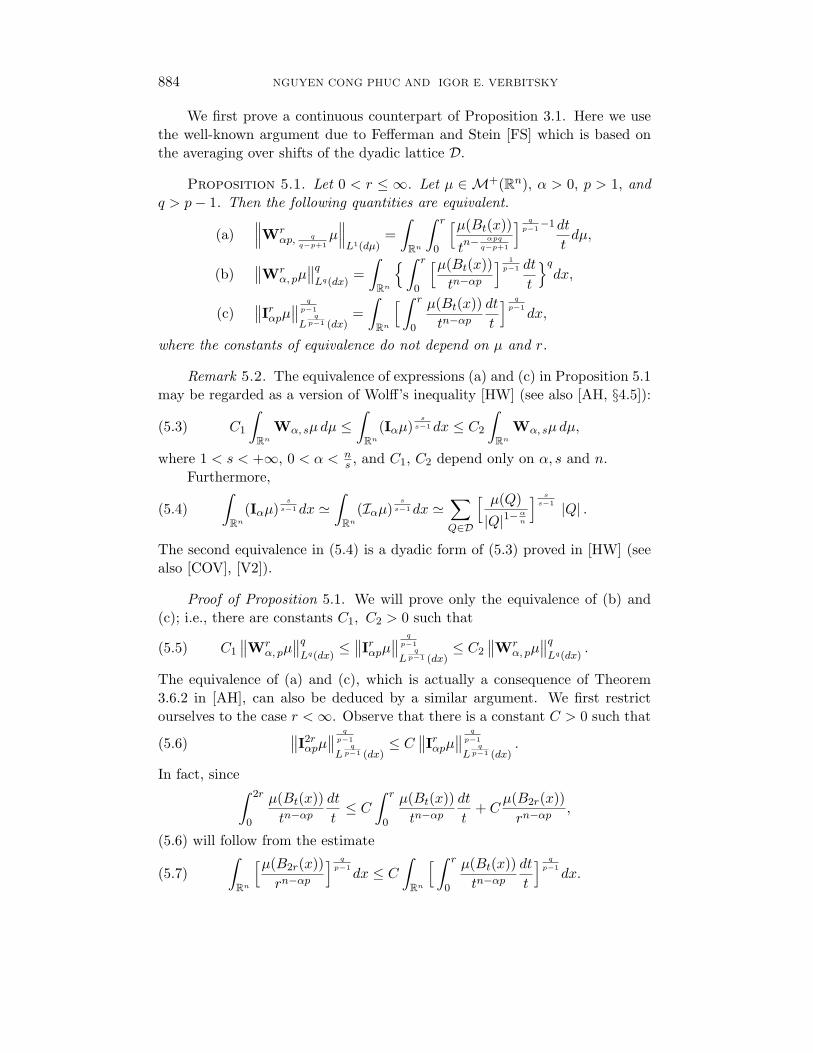
Proposition 5.1. Let 0 < r ≤ ∞. Let µ ∈ M+(Rn), α > 0, p > 1, andq > p− 1. Then the following quantities are equivalent.
(a)∥∥∥Wr
αp, q
q−p+1µ∥∥∥L1(dµ)
=∫Rn
∫ r
0
[µ(Bt(x))
tn−αpq
q−p+1
] q
p−1−1dt
tdµ,
(b)∥∥Wr
α, pµ∥∥qLq(dx)
=∫Rn
∫ r
0
[µ(Bt(x))tn−αp
] 1p−1 dt
t
qdx,
(c)∥∥Irαpµ∥∥ q
p−1
Lqp−1 (dx)
=∫Rn
[ ∫ r
0
µ(Bt(x))tn−αp
dt
t
] q
p−1dx,
where the constants of equivalence do not depend on µ and r.
Remark 5.2. The equivalence of expressions (a) and (c) in Proposition 5.1may be regarded as a version of Wolff’s inequality [HW] (see also [AH, §4.5]):
(5.3) C1
∫Rn
Wα, sµdµ ≤∫Rn
(Iαµ)s
s−1dx ≤ C2
∫Rn
Wα, sµdµ,
where 1 < s < +∞, 0 < α < ns , and C1, C2 depend only on α, s and n.
Furthermore,
(5.4)∫Rn
(Iαµ)s
s−1dx '∫Rn
(Iαµ)s
s−1dx '∑Q∈D
[ µ(Q)|Q|1−
α
n
] s
s−1 |Q| .
The second equivalence in (5.4) is a dyadic form of (5.3) proved in [HW] (seealso [COV], [V2]).
Proof of Proposition 5.1. We will prove only the equivalence of (b) and(c); i.e., there are constants C1, C2 > 0 such that
(5.5) C1
∥∥Wrα, pµ
∥∥qLq(dx)
≤∥∥Irαpµ∥∥ q
p−1
Lqp−1 (dx)
≤ C2
∥∥Wrα, pµ
∥∥qLq(dx)
.
The equivalence of (a) and (c), which is actually a consequence of Theorem3.6.2 in [AH], can also be deduced by a similar argument. We first restrictourselves to the case r <∞. Observe that there is a constant C > 0 such that
(5.6)∥∥I2rαpµ∥∥ q
p−1
Lqp−1 (dx)
≤ C∥∥Irαpµ∥∥ q
p−1
Lqp−1 (dx)
.
In fact, since∫ 2r
0
µ(Bt(x))tn−αp
dt
t≤ C
∫ r
0
µ(Bt(x))tn−αp
dt
t+ C
µ(B2r(x))rn−αp
,
(5.6) will follow from the estimate
(5.7)∫Rn
[µ(B2r(x))rn−αp
] q
p−1dx ≤ C
∫Rn
[ ∫ r
0
µ(Bt(x))tn−αp
dt
t
] q
p−1dx.
QUASILINEAR AND HESSIAN EQUATIONS 885
Note that for a partition of Rn into a union of disjoint cubes Qj such thatdiam(Qj) = r
4 , ∫Rnµ(B2r(x))
q
p−1dx=∑j
∫Qj
µ(B2r(x))q
p−1dx
≤C∑j
∫Qj
µ(Qj)q
p−1dx,
where we have used the fact that the ball B2r(x) is contained in the union ofat most N cubes in Qj for some constant N depending only on n. Thus∫
Rn
[µ(B2r(x))rn−αp
] q
p−1dx≤C
∑j
∫Qj
[µ(Br/2(x))rn−αp
] q
p−1dx
≤C∑j
∫Qj
[ ∫ r
0
µ(Bt(x))tn−αp
dt
t
] q
p−1dx,
which gives (5.7).By arguing as in [COV, §3], we can find constants a, C and c depending
only on p and n such that
Wrα, pµ(x) ≤ Cr−n
∫|t|≤cr
∑Q∈Dt
`(Q)≤4 ra
[ µ(Q)
|Q|1−αp
n
] 1p−1χQ(x)dt,
where Dt, t ∈ Rn, denotes the lattice D + t = Q = Q′ + t : Q′ ∈ D and `(Q)is the side length of Q. Using Proposition 2.2 in [COV] and arguing as in theproof of Theorem 3.1 we obtain∫Rn
∑Q∈Dt
`(Q)≤4 ra
[ µ(Q)
|Q|1−αp
n
] 1p−1χQ(x)
qdx '
∫Rn
[ ∑Q∈Dt
`(Q)≤4 ra
µ(Q)
|Q|1−αp
n
χQ(x)] q
p−1dx,
where the constants of equivalence are independent of µ, r and t. The last twoestimates together with the integral Minkowski inequality then give
||Wrα, pµ||Lq(dx)≤Cr−n
∫|t|≤cr
∫Rn
( ∑Q∈Dt
`(Q)≤4 ra
[ µ(Q)
|Q|1−αp
n
] 1p−1χQ(x)
)qdx 1q
dt
≤Cr−n∫|t|≤cr
[ ∫Rn
( ∑Q∈Dt
`(Q)≤4 ra
µ(Q)
|Q|1−αp
n
χQ(x)) q
p−1dx] 1q
dt.
Note that ∑Q∈Dt
`(Q)≤4 ra
µ(Q)
|Q|1−αp
n
χQ(x)≤C∑
2k≤4 ra
µ(B(x,√n2k))
2k(n−αp)
≤CI8r√n
aαp µ(x)
886 NGUYEN CONG PHUC AND IGOR E. VERBITSKY
where C is independent of t. Thus, in view of (5.6), we obtain the lowerestimate in (5.5).
Now by letting R→∞ in the inequality
||WRα, pµ||
qLq(dx) ≤ C ||I
Rαpµ||
q
p−1
Lqp−1 (dx)
, 0 < R <∞,
we get the lower estimate in (5.5) with r = ∞. The upper estimate in (5.5)can be deduced in a similar way. This completes the proof of Proposition 5.1.
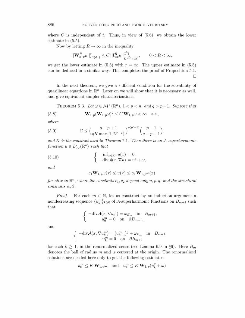
In the next theorem, we give a sufficient condition for the solvability ofquasilinear equations in Rn. Later on we will show that it is necessary as well,and give equivalent simpler characterizations.
Theorem 5.3. Let ω ∈M+(Rn), 1 < p < n, and q > p−1. Suppose that
(5.8) W1, p(W1, pω)q ≤ CW1, pω <∞ a.e.,
where
(5.9) C ≤( q − p+ 1qK max1, 2p′−2
)q(p′−1)( p− 1q − p+ 1
),
and K is the constant used in Theorem 2.1. Then there is an A-superharmonicfunction u ∈ Lqloc(R
n) such thatinfx∈Rn u(x) = 0,−divA(x,∇u) = uq + ω,
(5.10)
andc1W1, pω(x) ≤ u(x) ≤ c2 W1, pω(x)
for all x in Rn, where the constants c1, c2 depend only n, p, q, and the structuralconstants α, β.
Proof. For each m ∈ N, let us construct by an induction argument anondecreasing sequence umk k≥0 of A-superharmonic functions on Bm+1 suchthat
−divA(x,∇um0 ) = ωBm in Bm+1,
um0 = 0 on ∂Bm+1,
and −divA(x,∇umk ) = (umk−1)q + ωBm in Bm+1,
umk = 0 on ∂Bm+1
for each k ≥ 1, in the renormalized sense (see Lemma 6.9 in §6). Here Bmdenotes the ball of radius m and is centered at the origin. The renormalizedsolutions are needed here only to get the following estimates:
um0 ≤ KW1, pω and umk ≤ KW1, p(uqk + ω)
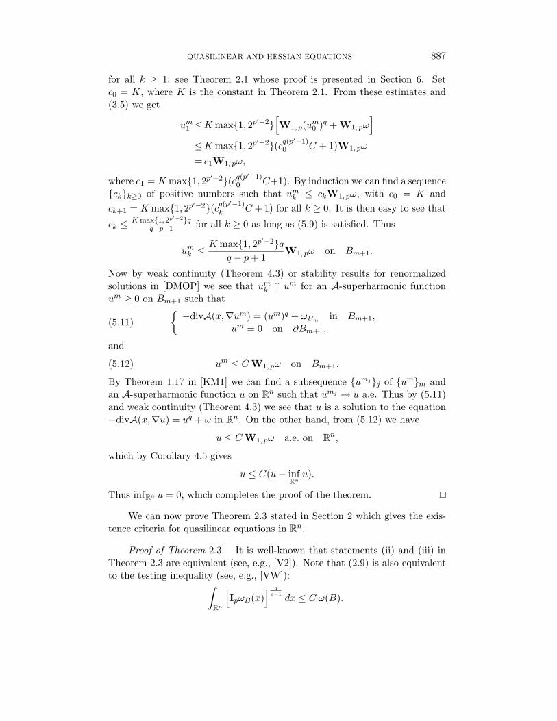
QUASILINEAR AND HESSIAN EQUATIONS 887
for all k ≥ 1; see Theorem 2.1 whose proof is presented in Section 6. Setc0 = K, where K is the constant in Theorem 2.1. From these estimates and(3.5) we get
um1 ≤K max1, 2p′−2[W1, p(um0 )q + W1, pω
]≤K max1, 2p′−2(cq(p
′−1)0 C + 1)W1, pω
= c1W1, pω,
where c1 = K max1, 2p′−2(cq(p′−1)
0 C+1). By induction we can find a sequenceckk≥0 of positive numbers such that umk ≤ ckW1, pω, with c0 = K andck+1 = K max1, 2p′−2(cq(p
′−1)k C + 1) for all k ≥ 0. It is then easy to see that
ck ≤ K max1, 2p′−2qq−p+1 for all k ≥ 0 as long as (5.9) is satisfied. Thus
umk ≤K max1, 2p′−2q
q − p+ 1W1, pω on Bm+1.
Now by weak continuity (Theorem 4.3) or stability results for renormalizedsolutions in [DMOP] we see that umk ↑ um for an A-superharmonic functionum ≥ 0 on Bm+1 such that
−divA(x,∇um) = (um)q + ωBm in Bm+1,
um = 0 on ∂Bm+1,(5.11)
and
(5.12) um ≤ CW1, pω on Bm+1.
By Theorem 1.17 in [KM1] we can find a subsequence umjj of umm andan A-superharmonic function u on Rn such that umj → u a.e. Thus by (5.11)and weak continuity (Theorem 4.3) we see that u is a solution to the equation−divA(x,∇u) = uq + ω in Rn. On the other hand, from (5.12) we have
u ≤ CW1, pω a.e. on Rn,
which by Corollary 4.5 gives
u ≤ C(u− infRnu).
Thus infRn u = 0, which completes the proof of the theorem.
We can now prove Theorem 2.3 stated in Section 2 which gives the exis-tence criteria for quasilinear equations in Rn.
Proof of Theorem 2.3. It is well-known that statements (ii) and (iii) inTheorem 2.3 are equivalent (see, e.g., [V2]). Note that (2.9) is also equivalentto the testing inequality (see, e.g., [VW]):∫
Rn
[IpωB(x)
] q
p−1dx ≤ C ω(B).
888 NGUYEN CONG PHUC AND IGOR E. VERBITSKY
By applying Proposition 5.1 we deduce (ii)⇒(iv). The implication (v)⇒(i)clearly follows from Theorem 5.3. Therefore, it remains to check (i)⇒(ii) and(iv)⇒(v).
Proof of (i)⇒(ii). Let u be a nonnegative solution of (2.8) and let µ =uq + εω. Then µ is a nonnegative measure such that µ ≥ uq, µ ≥ εω andu(x) ≥ CW1, pµ(x) by Corollary 4.5. Therefore,∫
Pdµ≥
∫Puq dx ≥ C
∫P
(W1, pµ)q dx
≥C∫P
[ ∑Q⊂P
( µ(Q)
|Q|1−p
n
) 1p−1χQ(x)
]qdx
for all dyadic cubes P in Rn. Using this and Proposition 3.1, we get∑Q⊂P
[ µ(Q)
|Q|1−p
n
] q
p−1 |Q| ≤ C µ(P ), P ∈ D.
It is known that the preceding condition is equivalent to the inequality (see[V1, §3])
‖Ip(f)‖L
qq−p+1 (dµ)
≤ C ‖f‖L
qq−p+1 (dx)
,
where C does not depend on f ∈ Lq
q−p+1 (dx). Since µ ≥ ε ω, we have
‖Ip(f)‖L
qq−p+1 (dω)
≤ εq−p+1−q C ‖f‖
Lq
q−p+1 (dx).
Therefore, by duality we obtain the testing inequality (2.9). This completesthe proof of (i)⇒(ii).
Proof of (iv)⇒(v). We first claim that (2.11) yields
(5.13)∫ ∞r
[ω(Bt(x))tn−p
] 1p−1 dt
t≤ C r
−pq−p+1 ,
where C is independent of x and r. Note that for y ∈ Bt(x) and τ ≥ 2t, wehave Bt(x) ⊂ Bτ (y). Thus,
W1, pωBt(x)(y)≥∫ ∞
2t
[ω(Bτ (y) ∩Bt(x))τn−p
] 1p−1 dτ
τ
≥C[ω(Bt(x))
tn−p
] 1p−1.
Combining this with (2.11) we obtain
(5.14) ω(Bt(x)) ≤ C tn−pq
q−p+1 ,
which clearly implies (5.13).
QUASILINEAR AND HESSIAN EQUATIONS 889
Next, we introduce a decomposition of the Wolff potential W1, p into its“upper” and “lower” parts, which are the continuous analogues of the discreteones given in (3.17) and (3.18) above:
Urµ(x) =∫ r
0
[µ(Bt(x))tn−p
] 1p−1 dt
t, r > 0, x ∈ Rn,
Lrµ(x) =∫ ∞r
[µ(Bt(x))tn−p
] 1p−1 dt
t, r > 0, x ∈ Rn.
Let dν = (W1, pω)qdx. For each r > 0 let dµr = (Urω)qdx and dλr =(Lrω)qdx. Then
ν ≤ C(q)(µr + λr).(5.15)
Let x ∈ Rn and Br = Br(x). Since W1, p(W1, pω)q = W1, pν, we have to provethat
W1, pν(x) =∫ ∞
0
[ν(Br)rn−p
] 1p−1 dr
r≤ CW1, pω(x).
For r > 0, t ≤ r and y ∈ Br we have Bt(y) ⊂ B2r. Therefore it is easy to seethat Urω = UrωB2r on Br. Using this together with (2.11), we have
µr(Br) =∫Br
(Urω)qdx =∫Br
(UrωB2r)qdx ≤ Cω(B2r).
Hence, ∫ ∞0
[µr(Br)rn−p
] 1p−1 dr
r≤C
∫ ∞0
[ω(B2r)rn−p
] 1p−1 dr
r(5.16)
≤C ′W1, pω(x).
On the other hand, for y ∈ Br and t ≥ r, we have Bt(y) ⊂ B2t, and conse-quently
Lrω(y)≤∫ ∞r
[ω(B2t)tn−p
] 1p−1 dt
t(5.17)
≤C∫ ∞
2r
[ω(Bt)tn−p
] 1p−1 dt
t
≤C Lrω(x).
Using (5.17), we obtain
λr(Br) =∫Br
(Lrω(y))qdy ≤ C(Lrω(x))qrn.
Thus, ∫ ∞0
[λr(Br)rn−p
] 1p−1 dr
r≤C ′
∫ ∞0
(Lrω(x))q
p−1 rp
p−1dr
r
=C ′∫ ∞
0
[ ∫ ∞r
(ω(Bt)tn−p
) 1p−1 dt
t
] q
p−1r
p
p−1dr
r
=C ′q
p
∫ ∞0
rp
p−1 [Lrω(x)]q
p−1−1[ω(Br)rn−p
] 1p−1 dr
r,
890 NGUYEN CONG PHUC AND IGOR E. VERBITSKY
where we have used integration by parts in the last equality. It then followsfrom (5.13) that∫ ∞
0
[λr(Br)rn−p
] 1p−1 dr
r≤C ′′
∫ ∞0
[ω(Br)rn−p
] 1p−1 dr
r(5.18)
=C ′′W1, pω(x).
Combining (5.15), (5.16) and (5.18) gives
W1, pν(x) =∫ ∞
0
[ν(Br)rn−p
] 1p−1 dr
r≤ CW1, pω(x)
for a suitable constant C independent of ω. Thus, (iv) implies (v) as claimedwhich completes the proof of the theorem.
6. Renormalized solutions of quasilinear Dirichlet problems
Let Ω be a bounded, open subset of Rn, n ≥ 2. We denote byMB(Ω) theset of all Radon measures with bounded variation on Ω. Recall that M+
B(Ω)denotes the set of nonnegative finite measures on Ω. Let A be as in Section 4,and let 1 < p <∞. In this section we consider the Dirichlet problem
−divA(x,∇u) = uq + ω,
u ≥ 0 in Ω,u = 0 on ∂Ω,
(6.1)
where ω ∈M+B(Ω) and q > p− 1.
It is well known that when the data are not regular enough, a solutionto nonlinear equations of Leray–Lions type does not necessarily belong to theSobolev space W1, p
0 (Ω). Therefore, we have to use the framework of renormal-ized solutions (see, e.g., [DMOP], [BMMP], [Gre], [Kil]).
For a measure µ inMB(Ω), its positive and negative parts are denoted byµ+ and µ−, respectively. We say that a sequence of measures µn inMB(Ω)converges in the narrow topology to µ ∈MB(Ω) if
limn→∞
∫Ωϕdµn =
∫Ωϕdµ
for every bounded and continuous function ϕ on Ω.Denote byM0(Ω) (respectivelyMs(Ω)) the set of all measures inMB(Ω)
which are absolutely continuous (respectively singular) with respect to thecapacity cap1, p(·,Ω). Here cap1, p(·,Ω) is the capacity relative to the domainΩ defined by
(6.2) cap1, p(E,Ω) = inf∫
Ω|∇φ|p dx : φ ∈ C∞0 (Ω), φ ≥ 1 on E
for any compact set E ⊂ Ω. Recall that, for every measure µ inMB(Ω), thereexists a unique pair of measures (µ0, µs) with µ0 ∈ M0(Ω) and µs ∈ Ms(Ω),
QUASILINEAR AND HESSIAN EQUATIONS 891
such that µ = µ0 + µs. If µ is nonnegative, then so are µ0 and µs (see [FST,Lemma 2.1]).
For k > 0 and for s ∈ R we denote by Tk(s) the truncation Tk(s) =max−k,mink, s. Recall also from [BBG] that if u is a measurable functionon Ω which is finite almost everywhere and satisfies Tk(u) ∈W 1, p
0 (Ω) for everyk > 0, then there exists a measurable function v : Ω→ Rn such that
∇Tk(u) = vχ|u|<k a.e. on Ω, for all k > 0.
Moreover, v is unique up to almost everywhere equivalence. We define thegradient Du of u as this function v, and set Du = v.
In [DMOP], several equivalent definitions of renormalized solutions aregiven. In what follows, we will need the following ones.
Definition 6.1. Let µ ∈ MB(Ω). Then u is said to be a renormalizedsolution of
−divA(x,∇u) = µ in Ω,u = 0 on ∂Ω,
(6.3)
if the following conditions hold:
(a) The function u is measurable and finite almost everywhere, and Tk(u)belongs to W 1, p
0 (Ω) for every k > 0.
(b) The gradient Du of u satisfies |Du|p−1 ∈ Lq(Ω) for all q < nn−1 .
(c) If w belongs to W 1, p0 (Ω)∩L∞(Ω) and if there exist w+∞ and w−∞ in
W 1, r(Ω) ∩ L∞(Ω), with r > n, such thatw = w+∞ a.e. on the set u > k,w = w−∞ a.e. on the set u < −k
for some k > 0, then
(6.4)∫
ΩA(x,Du) · ∇wdx =
∫Ωwdµ0 +
∫Ωw+∞dµ+
s −∫
Ωw−∞dµ−s .
Definition 6.2. Let µ ∈ MB(Ω). Then u is a renormalized solution of(6.3) if u satisfies (a) and (b) in Definition 6.1, and if the following conditionshold:
(c) For every k > 0 there exist two nonnegative measures in M0(Ω), λ+k
and λ−k , concentrated on the sets u = k and u = −k, respectively, suchthat λ+
k → µ+s and λ−k → µ−s in the narrow topology of measures.
(d) For every k > 0
(6.5)∫|u|<k
A(x,Du) · ∇ϕdx =∫|u|<k
ϕdµ0 +∫
Ωϕdλ+
k −∫
Ωϕdλ−k
for every ϕ in W1, p0 (Ω) ∩ L∞(Ω).
892 NGUYEN CONG PHUC AND IGOR E. VERBITSKY
Remark 6.3. By [DMOP, Remark 2.18], if u is a renormalized solutionof (6.3) then (the cap1, p-quasi continuous representative of) u is finite cap1, p-quasieverywhere. Therefore, u is finite µ0-almost everywhere.
Remark 6.4. By (6.5), if u is a renormalized solution of (6.3) then
(6.6) −divA(x,∇Tk(u)) = µk in Ω,
whereµk = χ|u|<kµ0 + λ+
k − λ−k .
Since Tk(u) ∈ W 1, p0 (Ω), by (4.3) we see that −divA(x,∇Tk(u)) and hence µk
belong to the dual space W−1, p′(Ω) of W 1, p0 (Ω). Moreover, by Remark 6.3,
|u| <∞ µ0-almost everywhere and hence χ|u|<k → χΩ µ0-almost everywhereas k →∞. Therefore, by the monotone convergence theorem, µk converges toµ in the narrow topology of measures.
Remark 6.5. If µ ≥ 0, i.e., µ ∈ M+B(Ω), and u is a renormalized solution
of (6.3) then u is nonnegative. To see this, for each k > 0 we “test” (6.4) withw = Tk(minu, 0), w+∞ = 0 and w−∞ = −k:∫
ΩA(x,Du) · ∇wdx =
∫Ωwdµ0 +
∫Ωkdµ−s =
∫Ωwdµ0 ≤ 0,
since µ−s = 0 and w ≤ 0. Thus using (4.3) we get∫Ω|∇Tk(minu, 0)|pdx ≤ 0
for every k > 0. Therefore minu, 0 = 0 a.e., i.e., u is nonnegative.
Remark 6.6. Let µ ∈M+B(Ω) and let u be a renormalized solution of (6.3).
Since u− = 0 a.e. (by Remark 6.5) and hence u− = 0 cap1,p-quasi everywhere(see [HKM, Th. 4.12]), in Remark 6.4 we may take λ−k = 0, and thus µk isnonnegative. Hence by (6.6) and Proposition 4.1, the functions vk defined byvk(x) = ess lim infy→x Tk(u)(y) are A-superharmonic and increasing. UsingLemma 7.3 in [HKM], it is then easy to see that vk → v as k →∞ everywherein Ω for some A-superharmonic function v on Ω such that v = u a.e. In otherwords, v is an A-superharmonic representative of u.
Remark 6.7. When dealing with pointwise values of a renormalized so-lution u to (6.3) with measure data µ ≥ 0, we always identify u with itsA-superharmonic representative mentioned in Remark 6.6.
We now establish a comparison principle for renormalized solutions.
QUASILINEAR AND HESSIAN EQUATIONS 893
Lemma 6.8. Let µ, ν ∈ M+B(Ω) be such that µ ≤ ν. Suppose that u and
v are renormalized solutions of−divA(x,∇u) = µ in Ω,
u = 0 on ∂Ω,
and −divA(x,∇v) = ν in Ω,
v = 0 on ∂Ω,
respectively. If u is uniformly bounded then u ≤ v.
Proof. Let w = min(u − v)+, k. Then w = 0 on the set v > k + Mand w = k on the set v < −k −M, where M = supΩ u. Moreover, w ∈W 1, p
0 ∩ L∞(Ω) as w = min(u − Tk+M (v))+, k. Thus by Definition 6.1 wehave
(6.7)∫
ΩA(x,Dv) · ∇wdx =
∫Ωwdν0.
On the other hand, since u is bounded (hence belongs to W 1, p0 (Ω)) we have
(6.8)∫
ΩA(x,Du) · ∇wdx =
∫Ωwdµ.
From (6.7) and (6.8) we get∫Ω
[A(x,Du)−A(x,Dv)] · ∇wdx ≤ 0.
Consequently,∫0<u−v<k
[A(x,Du)−A(x,Dv)] · (Du−Dv)dx ≤ 0,
since ∇w = ∇maxTk(u − v), 0 = D(u − v)χ0<u−v<k. Thus by (4.4) wehave ∇w = 0 and hence w = 0 a.e. for every k > 0, which gives u ≤ v.
In the following lemma we drop the assumption that u is uniformly boundedin Lemma 6.8, but claim only the existence of v such that v ≥ u. This lemmawas referred to in the proof of Theorem 5.3 given in Section 5 above.
Lemma 6.9. Let µ, ν ∈ M+B(Ω) be such that ν ≥ µ. Suppose that u is a
renormalized solution of−divA(x,∇u) = µ in Ω,
u = 0 on ∂Ω.
Then there exists v ≥ u such that−divA(x,∇v) = ν in Ω,
v = 0 on ∂Ω
in the renormalized sense.
894 NGUYEN CONG PHUC AND IGOR E. VERBITSKY
Proof. Let uk = minu, k for each k ∈ N. From Definition 6.2 ofrenormalized solutions we have
−divA(x,∇uk) = µ0u<k + λ+k in Ω,
uk = 0 on ∂Ω
in the renormalized sense for a sequence of nonnegative measures λ+k that
converges to µ+s in the narrow topology of measures. Thus, by Lemma 6.8 we
have uk ≤ vk, where vk are renormalized solutions of−divA(x,∇vk) = µ0 + λ+
k + ν − µ in Ω,vk = 0 on ∂Ω.
Finally, it follows from the stability results in [DMOP] that we can find asubsequence of vk that converges a.e. to a required function v.
We will also need the following version of Lemma 6.9 which will be usedin the proof of Theorem 2.1 on global potential estimates for renormalizedsolutions stated in Section 2.
Lemma 6.10. Suppose that u is a renormalized solution to (6.3) with dataµ ∈M+
B(Ω). Let B be a ball that contains Ω. Then there exists a renormalizedsolution w on B to
(6.9)−divA(x,∇w) = µ in B,
w = 0 on ∂B
such that u ≤ w on Ω, and
||w||Lp−1(B) ≤ CRp
p−1µ(Ω)1p−1 .(6.10)
Proof. Let uk = minu, k, k > 0, and let µk = χu<kµ0 + λ+k be as in
Remark 6.4 (note that λ−k = 0 by Remark 6.6). We see that uk ∈ W 1,p0 (Ω) is
the unique solution of problem (6.3) with data µk. We next extend uk by zerooutside Ω, and set
Ψ = minwk − uk, 0 = minminwk, k − uk, 0,
where wk, k > 0, is a renormalized solution to the problem−divA(x,∇wk) = µ0 + λ+
k in B,
wk = 0 on ∂B.
QUASILINEAR AND HESSIAN EQUATIONS 895
Note that Ψ ∈W 1, p0 (Ω) ∩W 1, p
0 (B) ∩ L∞(B) since |Ψ| ≤ uk. Then using Ψ asa test function we have
0≥∫BA(x,∇wk) · ∇Ψdx−
∫ΩA(x,∇uk) · ∇Ψdx
=∫B∩wk<uk
A(x,∇wk) · ∇Ψdx−∫B∩wk<uk
A(x,∇uk) · ∇Ψdx
=∫B∩wk<uk
[A(x,∇wk)−A(x,∇uk)] · (∇wk −∇uk)dx.
Thus ∇wk = ∇uk a.e. on the set B ∩ wk < uk by hypothesis (4.4) on A.Hence Ψ = 0 a.e.; i.e.,
(6.11) uk ≤ wk a.e.
Now by the stability results for renormalized solutions established in[DMOP] we can find a subsequence wkj of wk such that wkj → w a.e.,where w is a renormalized solution to (6.9). By (6.11) we have u ≤ w a.e. onΩ, and hence u ≤ w everywhere on Ω due to Remark 6.7 and Proposition 4.1.
Finally, note that for p < n we have
||w||Ln(p−1)n−p ,∞
(B)≤ C µ(Ω)
1p−1 ,
for a constant C independent of R (see [DMOP, Th. 4.1] or [BBG, Lemma4.1]). Thus we obtain (6.10). Inequality (6.10) also holds for p ≥ n; see forexample [Gre, Lemma 2.1]. This completes the proof of the lemma.
Proof of Theorem 2.1. The lower estimate in (2.6) is just a restatement ofthe local estimate given in Theorem 4.4. To prove the upper estimate we letB = B2R(a), where R = diam(Ω), a ∈ Ω so that Ω ⊂ B. Also, let w be as inLemma 6.10 with respect to that choice of B. For x ∈ Ω we denote by d(x)the distance from x to the boundary ∂B of B. By Theorem 4.4, Lemma 6.10,and the fact that d(x) ≥ R,
u(x)≤w(x) ≤ CW23d(x)
1, p µ(x) + C infB 1
3 d(x)(x)w
≤CW2R1, pµ(x) + Cd(x)
−np−1 ||w||Lp−1(B)
≤CW2R1, pµ(x) + CR
−np−1 ||w||Lp−1(B).
Thus from (6.10) we get the desired upper estimate in (2.6).
We next give a sufficient condition for the existence of renormalized solu-tions to quasilinear equations in a bounded domain Ω, which is an analogueof Theorem 5.3 related to the case Ω = Rn. Its proof is based on stabilityresults for renormalized solutions in place of the weak continuity of measuresgenerated by A-superharmonic functions used in the proof of Theorem 5.3.
896 NGUYEN CONG PHUC AND IGOR E. VERBITSKY
Theorem 6.11. Let ω ∈M+B(Ω). Let p > 1 and q > p− 1. Suppose that
R = diam(Ω), and
W2R1, p (W2R
1, pω)q ≤ CW2R1, pω a.e.,
where
C ≤( q − p+ 1qK max1, 2p′−2
)q(p′−1)( p− 1q − p+ 1
),
and K is the constant in Theorem 2.1. Then there is a renormalized solutionu ∈ Lq(Ω) to the Dirichlet problem
−divA(x,∇u) = uq + ω in Ω,u = 0 on ∂Ω
(6.12)
such thatu(x) ≤M W2R
1, pω(x)
for all x in Ω, where the constant M depends only on p, q, n, and the structuralconstants α and β.
Proof. By Lemma 6.9 we can find a nondecreasing sequence ukk≥0 ofrenormalized solutions to the following Dirichlet problems:
−divA(x,∇u0) = ω in Ω,u0 = 0 on ∂Ω,
(6.13)
and −divA(x,∇uk) = uqk−1 + ω in Ω,
uk = 0 on ∂Ω(6.14)
for k ≥ 1. By Theorem 2.1 we have
u0 ≤ K W2R1, pω, uk ≤ K W2R
1, p(uqk−1 + ω).
Thus arguing as in the proof of Theorem 5.3, we obtain a constant M > 0 suchthat
uk ≤M W2R1, pω <∞ a.e.
for all k ≥ 0. Therefore, uk converges pointwise to a nonnegative function ufor which
u ≤M W2R1, pω <∞ a.e.,
and uqk → uq in L1(Ω). Finally, in view of (6.14), the stability result in [DMOP,Th. 3.4] asserts that u is a renormalized solution of (6.12), which proves thetheorem.
QUASILINEAR AND HESSIAN EQUATIONS 897
Let Q = Q be a Whitney decomposition of Ω, i.e., Q is a disjointsubfamily of the family of dyadic cubes in Rn such that Ω = ∪Q∈QQ, where wecan assume that 25diam(Q) ≤ dist(Q, ∂Ω) ≤ 27diam(Q). Let φQQ∈Q be apartition of unity associated with the Whitney decomposition of Ω above: 0 ≤φQ ∈ C∞0 (Q∗), φQ ≥ 1/C(n) onQ,
∑Q φQ = 1 and |DγφQ| ≤ Aγ(diam(Q))−|γ|
for all multi-indices γ. Here Q∗ = (1 + ε)Q, 0 < ε < 14 and C(n) is a positive
constant depending only on n such that each point in Ω is contained in at mostC(n) of the cubes Q∗ (see [St1]).
The following theorem is an extension of Theorem 2.16 on local estimatesfor solutions of quasilinear equations.
Theorem 6.12. Let ω be a locally finite, nonnegative measure on an open(not necessarily bounded) set Ω. Let p > 1 and q > p− 1. Suppose that thereexists a nonnegative A-superharmonic function u in Ω such that
−divA(x,∇u) = uq + ω in Ω.
Then, for each cube P ∈ Q and compact set E ⊂ Ω,
(6.15) µP (E) ≤ C CapIp,q
q−p+1(E)
if pqq−p+1 < n, and
µP (E) ≤ C(P ) CapGp,q
q−p+1(E)(6.16)
if pqq−p+1 ≥ n. Here dµ = uqdx+dω, and the constant C in (6.15) is independent
of P ∈ Q and E ⊂ Ω, but the constant C(P ) in (6.16) may depend on the sidelength of P .
Moreover, if pqq−p+1 < n and Ω is a bounded C∞-domain, then
µ(E) ≤ C capp, q
q−p+1(E,Ω)
for all compact sets E ⊂ Ω, where capp, q
q−p+1(E,Ω) is defined by (2.24).
Proof. Let P be a fixed dyadic cube in Q. For a dyadic cube P ′ ⊂ P wehave
for all x ∈ P ′. Thus it follows from Proposition 3.1 that
(6.17)∑Q⊂P ′
[ µ(Q)
|Q|1−p
n
] q
p−1 |Q| ≤ C∫P ′uqdx ≤ Cµ(P ′), P ′ ⊂ P.
Hence
(6.18) µ(P ′) ≤ C∣∣P ′∣∣1− pq
n(q−p+1) , P ′ ⊂ P.
To get a better estimate for µ(P ′) in the case pqq−p+1 = n, we observe that
(6.17) is a dyadic Carleson condition. Thus by the dyadic Carleson imbeddingtheorem (see, e.g., [NTV], [V1]) we obtain, for pq
q−p+1 = n,
(6.19)∑Q⊂P
µ(Q)q
p−1
[ 1µ(Q)
∫Qfdµ
] q
p−1 ≤ C∫Pf
q
p−1dµ,
where f ∈ Lq
p−1 (dµP ), f ≥ 0. From (6.19) with f = χP ′ , one gets
(6.20) µ(P ′) ≤ C(
log2n |P ||P ′|
) 1−pq−p+1
, P ′ ⊂ P,
if pqq−p+1 = n. Now let P ′ be a dyadic cube in Rn. From Wolff’s inequality
(5.4) we have∫Rn
(IpµP ′∩P )q
p−1dx(6.21)
≤ C∑Q∈D
[µP (P ′ ∩Q)
|Q|1−p
n
] q
p−1 |Q|
= C∑Q⊂P ′
[ µP (Q)
|Q|1−p
n
] q
p−1 |Q|+ C∑P ′ Q
[µP (P ′)
|Q|1−p
n
] q
p−1 |Q| .
Thus, for pqq−p+1 < n, by combining (6.17) and (6.21) we deduce
(6.22)∫Rn
(IpµP ′∩P )q
p−1 dx ≤ C µP (P ′).
In the case pqq−p+1 ≥ n, a similar argument using (6.17), (6.18), (6.20) and
Wolff’s inequality for Bessel potentials:∫Rn
(GpµP ′∩P )q
p−1dx ≤ C(P )∑
Q∈D, Q⊂P
[µP (P ′ ∩Q)
|Q|1−p
n
] q
p−1 |Q| ,
(see [AH, §4.5]), also gives
(6.23)∫Rn
(GpµP ′∩P )q
p−1dx ≤ C(P )µP (P ′),
where the constant C(P ) may depend on the side length of P . Note that (6.22)which holds for all dyadic cubes P ′ in Rn is the well-known Kerman-Sawyercondition. Therefore by the results of [KS],
‖Ipf‖L qq−p+1 (dµP )
≤ C ‖f‖L
qq−p+1 (dx)
QUASILINEAR AND HESSIAN EQUATIONS 899
for all f ∈ Lq
q−p+1 (Rn) which is equivalent to the capacitary condition
µP (E) ≤ C CapIp,q
q−p+1(E)
for all compact sets E ⊂ Rn. Thus we obtain (6.15). The inequality (6.16)is proved in the same way using (6.23). From (6.15) and the definition ofcapp, q
q−p+1(·,Ω), we see that, for each cube P ∈ Q,
µP (E) ≤ Ccapp, q
q−p+1(E ∩ P,Ω)
for all compact sets E ⊂ Ω. Thus
µ(E)≤∑P∈Q
µP (E)
≤C∑P∈Q
capp, q
q−p+1(E ∩ P,Ω)
≤C capp, q
q−p+1(E,Ω),
where the last inequality follows from the quasi-additivity of the capacitycapp, q
q−p+1(·,Ω) which is considered in the next theorem.
Let BR be a ball such that B2R ⊂ Ω. It is easy to see that there exists aconstant c > 0 such that `(P ) ≥ cR for any Whitney cube P that intersectsBR. On the other hand, if Br is a ball in BR then we can find at most Ndyadic cubes Pi with c r4 ≤ `(Pi) < c r2 that cover Br, where N depends onlyon n. Thus we can deduce from (6.20) the following corollary which gives animproved estimate in the critical case q = n(p−1)
n−p , 1 < p < n.
Corollary 6.13. Let ω, Ω, p, q and u be as in Theorem 6.12. Then inthe case pq
q−p+1 = n, ∫Br
uq dx+ ω(Br) ≤ C(log 2Rr )
1−pq−p+1
for all balls Br ⊂ BR such that B2R ⊂ Ω.
Theorem 6.14. Suppose that Ω is a C∞-domain in Rn. Then there existsa constant C > 0 such that∑
Q∈Qcapp, q
q−p+1(E ∩Q,Ω) ≤ Ccapp, q
q−p+1(E,Ω)
for all compact sets E ⊂ Ω.
Proof. Obviously, we may assume that capp, q
q−p+1(E,Ω) > 0. Then by
definition there exists f ∈ C∞0 (Ω), f ≥ 1, on E such that
2 capp, q
q−p+1(E,Ω) ≥ ‖f‖
q
q−p+1
Wp,
qq−p+1 (Rn)
.
900 NGUYEN CONG PHUC AND IGOR E. VERBITSKY
By the refined localization principle on the smooth domain Ω for the functionspace W p, q
q−p+1 (see, e.g., [Tri, Th. 5.14]) we have
‖f‖q
q−p+1
Wp,
qq−p+1 (Rn)
≥ C∑Q∈Q‖fφQ‖
q
q−p+1
Wp,
qq−p+1 (Rn)
.
Thus
(6.24)∑Q∈Q‖fφQ‖
q
q−p+1
Wp,
qq−p+1 (Rn)
≤ Ccapp, q
q−p+1(E,Ω).
Note that for x ∈ E ∩Q,
fφQ ≥ φQ ≥ 1/C(n).
Hence by definition we have
capp, q
q−p+1(E ∩Q,Ω) ≤ C ‖fφQ‖
q
q−p+1
Wp,
qq−p+1 (Rn)
.
From this and (6.24) we deduce the desired inequality.
We now prove Theorem 2.10 stated in Section 2. which gives existencecriteria for quasilinear equations in a bounded domain.
Proof of Theorem 2.10. Since ω is compactly supported in Ω, we have(i)⇒(ii) by Theorem 6.12. Thus we need to show (ii)⇒(iii)⇒(iv) ⇒(i). Notethat the capacitary inequality (2.20) is equivalent to the Kerman–Sawyer con-dition
(6.25)∫Rn
[GpωB(x)
] q
p−1dx ≤ C ω(B),
(see [KS], [V2]). Note also that
(6.26)∫Rn
[Gpµ(x)
] q
p−1dx '
∫Rn
[ ∫ 2R
0
µ(Bt(x))tn−p
] q
p−1dx,
where the constants of equivalence are independent of the measure µ, (see[HW], [AH]). Thus from (6.25), (6.26), and Proposition 5.1 we deduce theimplication (ii)⇒(iii). By Theorem 6.11 we have (iv)⇒(i). It remains to showthat (iii)⇒(iv). In fact, the proof of this implication is similar to the proofof (iv)⇒(v) in Theorem 2.3. We will only sketch some crucial steps here. Wedefine the “lower” and “upper” parts of the truncated Wolff’s potential W2R
1, p
respectively by
L2Rr µ(x) =
∫ 2R
r
[µ(Bt(x))tn−p
] 1p−1 dt
t, 0 < r < 2R, x ∈ Rn,
and
U2Rr µ(x) =
∫ r
0
[µ(Bt(x))tn−p
] 1p−1 dt
t, 0 < r < 2R, x ∈ Rn.
QUASILINEAR AND HESSIAN EQUATIONS 901
Since R = diam(Ω) and ω ∈ M+B (Ω), to prove (2.22), it is enough to verify
that, for x ∈ Ω,
(6.27)∫ 2R
0
[µr(Br(x))rn−p
] 1p−1 dr
r≤ CW2R
1, pω(x),
and
(6.28)∫ 2R
0
[λr(Br(x))rn−p
] 1p−1 dr
r≤ CW2R
1, pω(x),
where dµr = (U2Rr ω)qdx, dλr = (L2R
r ω)qdx and 0 < r < 2R. The proof of(6.27) is the same as before. For the proof of (6.28), we need an estimatesimilar to (5.13) in the proof of Theorem 2.3, namely,
(6.29)∫ 4R
r
[ω(Bt(x))tn−p
] 1p−1 dt
t≤ C(R,ω(Ω)) r
−pq−p+1
for all 0 < r ≤ 4R and x ∈ Ω. In fact, note that for 0 < t < R2 and y ∈ Bt(x),
W2R1, pωBt(x)(y)≥
∫ 2R
2t
[ω(Bτ (y) ∩Bt(x))τn−p
] 1p−1 dτ
τ
≥C(n, p)[ω(Bt(x))
tn−p
] 1p−1.
As before, from this inequality and (2.21) we get
(6.30) ω(Bt(x)) ≤ Ctn−pq
q−p+1 , 0 < t < R2 .
To prove (6.29), we can assume that 0 < r < R2 and write the left-hand side
of (6.29) in the form
(6.31)∫ R
2
r
[ω(Bt(x))tn−p
] 1p−1 dt
t+∫ 4R
R
2
[ω(Bt(x))tn−p
] 1p−1 dt
t.
Applying (6.30) to the first term of (6.31) and using the fact that ω ∈M+B(Ω)
in the second term of (6.31), we finally obtain (6.29). This completes the proofof (iii)⇒(iv), and hence Theorem 2.10 is proved.
We are now in a position to obtain the characterization of removablesingularities for homogeneous quasilinear equations in Theorem 2.18 above.
Proof of Theorem 2.18. Let us first prove the “only if” part of thetheorem. Suppose that CapGp,
q
q−p+1(E) = 0, and u is a solution of (2.25).
We have cap1, p(E,Ω) = 0, where the capacity cap1, p(·,Ω) is defined by (6.2).Thus u can be extended so that it is a nonnegative A-superharmonic functionin Ω (see [HKM]). Let µ[u] be the Radon measure on Ω associated with u, andlet ϕ be an arbitrary nonnegative function in C∞0 (Ω). As in [BP, Lemme 2.2],we can find a sequence ϕn of nonnegative functions in C∞0 (Ω \E) such that
(6.32) 0 ≤ ϕn ≤ ϕ; ϕn → ϕ CapGp,q
q−p+1-quasi everywhere.
902 NGUYEN CONG PHUC AND IGOR E. VERBITSKY
By Fatou’s lemma we have∫Ωuq ϕdx≤ lim inf
n→∞
∫Ωuq ϕn dx
= lim infn→∞
∫Ωϕn dµ[u]
≤∫
Ωϕdµ[u] <∞.
Therefore u ∈ Lqloc(Ω), and µ[u] ≥ uq in D′(Ω). It is then easy to see that
−divA(x,∇u) = uq + µE in D′(Ω)
for some nonnegative measure µE such that µE(A) = 0 for any Borel setA ⊂ Ω \ E. Moreover, by Theorem 6.12 we have
µE(E) ≤ C(E) CapGp,q
q−p+1(E) = 0.
Thus µE = 0 and u solves (2.25) with Ω in place of Ω \ E.The “if” part of the theorem is proved in the same way as in the linear
case p = 2 using the existence results obtained in Theorem 2.10. We refer to[AP] for details.
7. Hessian equations
In this section, we study a fully nonlinear counterpart of the theory pre-sented in the previous sections. Here the notion of k-subharmonic(k-convex) functions associated with the fully nonlinear k-Hessian operatorFk, k = 1, . . . , n, introduced by Trudinger and Wang in [TW1]–[TW3] willplay a role similar to that of A-superharmonic functions in the quasilinear the-ory.
Let Ω be an open set in Rn, n ≥ 2. For k = 1, . . . , n and u ∈ C2(Ω), thek-Hessian operator Fk is defined by
Fk[u] = Sk(λ(D2u)),
where λ(D2u) = (λ1, . . . , λn) denotes the eigenvalues of the Hessian matrix ofsecond partial derivatives D2u, and Sk is the kth symmetric function on Rn
given bySk(λ) =
∑1≤i1<···<ik≤n
λi1 · · ·λik .
Thus F1[u] = ∆u and Fn[u] = detD2u. Alternatively, we may also write
Fk[u] = [D2u]k,
where for an n × n matrix A, [A]k is the k-trace of A, i.e., the sum of itsk×k principal minors. Several equivalent definitions of k-subharmonicity weregiven in [TW2], one of which involves the language of viscosity solutions: An
QUASILINEAR AND HESSIAN EQUATIONS 903
upper-semicontinuous function u : Ω → [−∞,∞) is said to be k-subharmonicin Ω, 1 ≤ k ≤ n, if Fk[q] ≥ 0 for any quadratic polynomial q such that u−q hasa local finite maximum in Ω. Equivalently, an upper-semicontinuous functionu : Ω→ [−∞,∞) is k-subharmonic in Ω if, for every open set Ω′ b Ω and forevery function v ∈ C2
loc(Ω′) ∩ C0(Ω′) satisfying Fk[v] ≥ 0 in Ω′, the following
implication holds:u ≤ v on ∂Ω′ =⇒ u ≤ v in Ω′,
(see [TW2, Lemma 2.1]). Note that a function u ∈ C2loc(Ω) is k-subharmonic
if and only ifFj [u] ≥ 0 in Ω for all j = 1, . . . , k.
We denote by Φk(Ω) the class of all k-subharmonic functions in Ω which arenot identically equal to −∞ in each component of Ω. It was proved in [TW2]that Φn(Ω) ⊂ Φn−1(Ω) · · · ⊂ Φ1(Ω) where Φ1(Ω) coincides with the set of allproper classical subharmonic functions in Ω, and Φn(Ω) is the set of functionsconvex on each component of Ω.
The following weak convergence result proved in [TW2] is fundamental topotential theory associated with k-Hessian operators.
Theorem 7.1 ([TW2]). For each u ∈ Φk(Ω), there exists a nonnegativeBorel measure µk[u] in Ω such that
(i) µk[u] = Fk[u] for u ∈ C2(Ω), and
(ii) if um is a sequence in Φk(Ω) converging in L1loc(Ω) to a function u ∈
Φk(Ω), then the sequence of the corresponding measures µk[um] convergesweakly to µk[u].
The measure µk[u] in the theorem above is called the k-Hessian measureassociated with u. Due to (i) in Theorem 7.1 we sometimes write Fk[u] in placeof µk[u] even in the case where u ∈ Φk(Ω) does not belong to C2(Ω). Thek-Hessian measure is an important tool in potential theory for Φk(Ω). It wasused by D. A. Labutin to derive pointwise estimates for functions in Φk(Ω) interms of Wolff’s potential, which is an analogue of Wolff’s potential estimatesfor A-superharmonic functions considered in Theorem 4.4.
Theorem 7.2 ([L]). Let u ≥ 0 be such that −u ∈ Φk(B3r(x)), where1 ≤ k ≤ n. If µ = µk[−u] then
C1Wr
82kk+1
, k+1µ(x) ≤ u(x) ≤ C2 inf
B(x,r)u+ C3W2r
2kk+1
, k+1µ(x),
where the constants C1, C2 and C3 depend only on n and k.
The following global estimate is deduced from the preceding theorem asin the quasilinear case.
904 NGUYEN CONG PHUC AND IGOR E. VERBITSKY
Corollary 7.3. Let u ≥ 0 be such that −u ∈ Φk(Rn), where 1 ≤ k < n2 .
If µ = µk[−u] and infRn u = 0 then for all x ∈ Rn,
1K
W 2kk+1
, k+1µ(x) ≤ u(x) ≤ KW 2kk+1
, k+1µ(x),
for a constant K depending only on n and k.
Let Ω be a bounded uniformly (k − 1)-convex domain in Rn, that is,∂Ω ∈ C2 and Hj(∂Ω) > 0, j = 1, ..., k − 1, where Hj(∂Ω) denotes the j-mean curvature of the boundary ∂Ω. We consider the following fully nonlinearproblem:
Fk[−u] = uq + ω in Ω,u ≥ 0 in Ω,u = ϕ on ∂Ω
(7.1)
in the class of functions u such that −u is k-subharmonic in Ω. Here ω isa nonnegative finite Borel measure which is regular enough near ∂Ω so thatthe boundary condition in (7.1) can be understood in the classical sense (see[TW1], [TW2]). Characterizations of the existence of u ≥ 0, −u ∈ Φk(Ω),continuous near ∂Ω, which solves (7.1), can be obtained using the iterationscheme employed in the proof of Theorem 6.11 along with weak continuity ofHessian measures and testing inequalities analogous to those used in the proofof Theorem 2.10. For this purpose, we first prove an extension of Theorem 2.2concerning the global potential estimates on a bounded domain, which is ananalogue of Theorem 2.1 established for quasilinear operators.
Theorem 7.4. Suppose that ϕ ≥ 0, ϕ ∈ C0(∂Ω) and ν = µ + f whereµ ∈ M+(Ω) has compact support in Ω and f ≥ 0, f ∈ Ls(Ω) with s > n
2k if1 ≤ k ≤ n
2 , and s = 1 if n2 < k ≤ n. Let u ≥ 0, −u ∈ Φk(Ω) be such that u is
continuous near ∂Ω and solvesµk[−u] = ν in Ω,u = ϕ on ∂Ω.
Then for all x ∈ Ω,
u(x) ≤ K[W2R
2kk+1
, k+1ν(x) + max∂Ω
ϕ],
where R = diam(Ω) and K is a constant depending only on n and k.
Proof. Suppose that the support of µ is contained in Ω′ for some openset Ω′ b Ω. Let M = supΩ\Ω′ u and um = minu,m for m > M . Then−um ∈ Φk(Ω), continuous near ∂Ω, solves
µk[−um] = νm in Ω,um = ϕ on ∂Ω
QUASILINEAR AND HESSIAN EQUATIONS 905
for certain nonnegative Borel measures νm in Ω. Since um → u in L1loc(Ω), by
Theorem 7.1 we have
(7.2) µm → ν = µ+ f weakly as measures in Ω.
Note that um = u in Ω \ Ω′ since m > M . Thus νm = µk[u] = f in Ω \ Ω′ forall m > M . Using this and (7.2) it is easy to see that∫
Ωφdµm →
∫Ωφdµ+
∫Ωφfdx
as m→∞ for all φ ∈ C0(Ω), i.e.,
µm → ν = µ+ f in the narrow topology of measures.
We now take a ball B = B2R(a) where a ∈ Ω so that Ω ⊂ B, and considersolutions wm ≥ 0, −wm ∈ Φk(B), continuous near ∂B, of
µk[−wm] = νm in B,
wm = max∂Ω ϕ on ∂B,
where m > M . Since um is bounded in Ω the measure νm is absolutely con-tinuous with respect to the capacity capk(·,Ω), and hence with respect tothe capacity capk(·, B) (see [TW3]). Here capk(·,Ω) is the k-Hessian capac-ity defined by (2.27). By a comparison principle (see [TW3, Th. 4.1]), wehave wm ≥ max∂Ω ϕ in B, and hence wm ≥ um on ∂Ω. Thus, applying thecomparison principle again, we have
wm ≥ um in Ω.(7.3)
Since νm → ν in the narrow topology of measures in Ω, we see that νm → ν
weakly as measures in B. Therefore, arguing as in [TW2, §6] we can find asubsequence wmj
such that wmj→ w a.e. for some w ≥ 0, −w ∈ Φk(B),
such that w is continuous near ∂B andµk[−w] = ν in B,
w = max∂Ω ϕ on ∂B.
Note that from (7.3), w ≥ u a.e. on Ω and hence w ≥ u everywhere onΩ. Using this and Theorem 7.2 applied to the function w on Bd(x)(x), whered(x) = dist(x, ∂B) we have, for x ∈ Ω,
u(x)≤CW2R2kk+1
, k+1ν(x) + C infB 1
3 d(x)(x)w(7.4)
≤CW2R2kk+1
, k+1ν(x) + C d(x)−n∫B 1
3 d(x)(x)w dy
≤C(W2R
2kk+1
, k+1ν(x) + max∂Ω
ϕ+R2−nk ν(Ω)
1k
),
906 NGUYEN CONG PHUC AND IGOR E. VERBITSKY
where the last inequality in (7.4) follows from the estimate (6.3) in [TW2].The proof of Theorem 7.4 is then completed by noting that∫ 2R
R
[ν(Bt(x))tn−2k
] 1k dt
t≥ CR2−n
k ν(Ω)1k
for all x ∈ Ω.
The following lemma is an analogue of Lemma 6.9. It is needed in theproof of Theorem 7.6 below to construct a solution to Hessian equations.
Lemma 7.5. Let Ω, ν, ϕ and u be as in Theorem 7.4. Let ν ′ be a measurewhich belongs to the same class as ν, i.e., ν ′ = µ′+ f ′, where µ′ ∈M+(Ω) hascompact support in Ω and f ′ ≥ 0, f ′ ∈ Ls(Ω) with s > n
2k if 1 ≤ k ≤ n2 , and
s = 1 if n2 < k ≤ n. Then there exists w ≥ u such that −w ∈ Φk(Ω) and
µk[−w] = ν + ν ′ in Ω,w = ϕ on ∂Ω.
Proof. By approximation we may assume that µ′ is absolutely continuouswith respect to the capacity capk(·,Ω). Let um and νm be as in the proof ofTheorem 7.4. Then by the comparison principle in [TW3, Th. 4.1], we haveum ≤ wm where wm is the solution of
µk[−wm] = νm + ν ′ in Ω,wm = ϕ on ∂Ω.
Thus arguing as in [TW2, §6] we obtain a subsequence wmj that converges
a.e. to a required function w.
From Lemma 7.5 and Theorem 2.2, along with the weak continuity ofHessian measures (Theorem 7.1), we deduce the following existence theoremfor fully nonlinear equations whose proof, which we will omit, is analogous tothat of Theorem 5.3 in the quasilinear case.
Theorem 7.6. Let ω ∈M+(Rn), 1 ≤ k < n2 , and q > k. Suppose that
W 2kk+1
, k+1 (W 2kk+1
, k+1ω)q ≤ CW 2kk+1
, k+1ω <∞ a.e.,
where
C ≤(q − kqK
)q/k k
q − k,
and K is the constant in Theorem 2.2. Then there exists u ≥ 0, u ∈ Lqloc(Rn),
such that −u ∈ Φk(Rn) and infx∈Rn u(x) = 0,Fk[−u] = uq + ω.
QUASILINEAR AND HESSIAN EQUATIONS 907
Moreover, u satisfies the two-sided estimate
c1W 2kk+1
, k+1ω(x) ≤ u(x) ≤ c2 W 2kk+1
, k+1ω(x)
for all x in Rn, where the constants c1, c2 depend only on n, k, q.
We are now in a position to establish the main results of this section.
Proof of Theorem 2.6. The proof of Theorem 2.6 is completely analogousto that of Theorem 2.3 in the quasilinear case using W 2k
k+1, k+1 in place of W1, p
and Theorem 7.6 in place of Theorem 5.3.
The proof of our next theorem on the existence of solutions for Hessianequations with nonhomogeneous boundary condition is similar to that of The-orem 6.11. However, due to the inhomogeneity we will need to take care of theboundary term. Moreover, the weak continuity of Hessian measures is used inplace of the stability result for renormalized solutions in the quasilinear case.
Theorem 7.7. Let Ω be a bounded uniformly (k − 1)-convex domain inRn. Suppose that ω ∈ M+
B(Ω) such that ω = µ + f , where µ ∈ M+(Ω) hascompact support in Ω, and 0 ≤ f ∈ Ls(Ω) with s > n
2k if 1 ≤ k ≤ n2 and s = 1
if n2 < k ≤ n. Let q > k, R = diam(Ω) and 0 ≤ ϕ ∈ C0(∂Ω). Suppose that
(7.5) W2R2kk+1
, k+1 (W2R2kk+1
, k+1ω)q ≤ AW2R2kk+1
, k+1ω,
and
(7.6) (max∂Ω
ϕ)q
k−1 ≤ B
k
q
2R2|B1(0)|1k
,
where A, B are positive constants such that
(7.7) A ≤( q − k
3q−1q qK
) qk( k
q − k
), and B ≤
( q − k3q−1q qK
q
k
) qk( k
q − k
).
Here K is the constant in Theorem 7.4. Then there exists a function u ≥ 0,−u ∈ Φk(Ω) ∩ Lq(Ω), continuous near ∂Ω such that
(7.8)Fk[−u] = uq + ω in Ω,
u = ϕ on ∂Ω.
Moreover, there is a constant C = C(n, k, q) such that
u ≤ CW2R
2kk+1
, k+1ω + W2R2kk+1
, k+1(max∂Ω
ϕ)q + max∂Ω
ϕ.
Proof. First observe by direct calculations that condition (7.6) is equiv-alent to
(7.9) W2R2kk+1
, k+1
[W2R
2kk+1
, k+1(max∂Ω
ϕ)q]q≤ BW2R
2kk+1
, k+1(max∂Ω
ϕ)q.
908 NGUYEN CONG PHUC AND IGOR E. VERBITSKY
From Lemma 7.5 it follows that we can choose inductively a nondecreasingsequence um of nonnegative functions on Ω such that
Fk[−u0] = ω in Ω,u0 = ϕ on ∂Ω,
and
(7.10)Fk[−um] = uqm−1 + ω in Ω,
um = ϕ on ∂Ω
for m ≥ 1. Here for each m ≥ 0, −um is k-subharmonic and is continuous near∂Ω. By Theorem 7.4 we have
u0≤KW2R2kk+1
, k+1ω +K max∂Ω
ϕ
= a0W2R2kk+1
, k+1ω + b0W2R2kk+1
, k+1(max∂Ω
ϕ)q +K max∂Ω
ϕ,
where a0 = K and b0 = 0. Thus
u1≤KW2R2kk+1
, k+1(uq0 + ω) +K max∂Ω
ϕ
≤K
(3q−1aq0)1kW2R
2kk+1
, k+1 (W2R2kk+1
, k+1ω)q
+(3q−1bq0)1kW2R
2kk+1
, k+1
[W2R
2kk+1
, k+1(max∂Ω
ϕ)q]q
+Kq
kW2R2kk+1
, k+1(max∂Ω
ϕ)q + W2R2kk+1
, k+1ω
+K max∂Ω
ϕ.
Then by (7.5) and (7.9),
u1≤K[(3q−1aq0)1kA+ 1]W2R
2kk+1
, k+1ω
+K[(3q−1bq0)1kB +K
q
k ]W2R2kk+1
, k+1(max∂Ω
ϕ)q +K max∂Ω
ϕ
= a1W2R2kk+1
, k+1ω + b1W2R2kk+1
, k+1(max∂Ω
ϕ)q +K max∂Ω
ϕ,
wherea1 = K[(3q−1aq0)
1kA+ 1], b1 = K[(3q−1bq0)
1kB +K
q
k ].
By induction we have
um ≤ amW2R2kk+1
, k+1ω + bmW2R2kk+1
, k+1(max∂Ω
ϕ)q +K max∂Ω
ϕ,
where
am+1 = K[(3q−1aqm)1kA+ 1], bm+1 = K[(3q−1bqm)
1kB +K
q
k ]
for all m ≥ 0. It is then easy to see that
am ≤Kq
q − k, and bm ≤
Kq
k+1q
q − k,
QUASILINEAR AND HESSIAN EQUATIONS 909
provided (7.7) is satisfied. Thus
um≤Kq
q − kW2R
2kk+1
, k+1ω(7.11)
+K
q
k+1q
q − kW2R
2kk+1
, k+1(max∂Ω
ϕ)q +K max∂Ω
ϕ.
Using (7.5) and (7.11) we see that um ↑ u for a function u ≥ 0 such that −u isk-subharmonic and uqm → uq in L1(Ω). Thus in view of (7.10) and Theorem7.1 we see that u is a desired solution of (7.8).
We will omit the proof of the next theorem, which contains Theorem 2.17in Section 2, as it is completely analogous to the proof of Theorem 6.12 in thequasilinear case.
Theorem 7.8. Let ω be a locally finite nonnegative measure on an open(not necessarily bounded) set Ω. Let 1 ≤ k ≤ n and q > k. Suppose that u ≥ 0,−u ∈ Φk(Ω), such that u is a solution to
Fk[−u] = uq + ω in Ω.
Then for each cube P ∈ Q, where Q = Q is a Whitney decomposition of Ω(see §6),
(7.12) µP (E) ≤ C CapI2k,q
q−k(E)
if 2kqq−k < n, and
(7.13) µP (E) ≤ C(P ) CapG2k,q
q−k(E)
if 2kqq−k ≥ n, for all compact sets E ⊂ Ω. Here dµ = uqdx+dω, and the constant
C in (7.12) does not depend on P ∈ Q and E ⊂ Ω; however, the constant C(P )in (7.13) may depend on the side length of P .
Moreover, if 2kqq−k < n, and Ω is a bounded C∞-domain then
µ(E) ≤ C cap2k, q
q−k(E,Ω)
for all compact sets E ⊂ Ω, where cap2k, q
q−k(E,Ω) is defined by (2.24).
Remark 7.9. Let BR be a ball such that B2R ⊂ Ω. Then in the criticalcase q = nk
n−2k , (k < n2 ), as in Corollary 6.13 we have
µ(Br) ≤ C(log 2Rr )
−kq−k
for all balls Br ⊂ BR.
We are now in a position to deduce Theorem 2.13 concerning the charac-terizations of solvability for Hessian equations in a bounded domain.
910 NGUYEN CONG PHUC AND IGOR E. VERBITSKY
Proof of Theorem 2.13. The proof of this theorem is analogous to thatof Theorem 2.6 in the quasilinear case. One only has to use Theorems 7.7 and7.8 in place of Theorems 6.11 and 6.12 respectively.
We next prove Theorem 2.19 on removable singularities for Hessian equa-tions.
Proof of Theorem 2.19. To prove this theorem, we will proceed as in theproof of Theorem 2.18. For the “only if” part, we may assume that k < n
2 ,since otherwise 2kq
q−k > n, and so E = ∅. Note that if CapG2k,q
q−k(E) = 0 then
CapG 2kk+1
, k+1(E) = 0 (see [AH, §5.5]), which implies that capk(E,Ω) = 0 due
to Theorem 2.20, whose proof is given below. Here capk(·,Ω) is the (relative)k-Hessian capacity associated with the domain Ω defined by (2.27). Thusby [L, Th. 4.2], E is a k-polar set, i.e., it is contained in the (−∞)-set of ak-subharmonic function in Rn. Suppose that u is a solution of (2.26). It iseasy to see that the function u defined by
(7.14) u(x) =
u(x), x ∈ Ω \ E,
lim infy→x, y 6∈E
u(y), x ∈ E
is an extension of u to Ω such that −u ∈ Φk(Ω). The rest of the proof is thenthe same as in the quasilinear case.
Finally, we prove Theorem 2.20 on the local equivalence of the k-Hessiancapacity and an appropriate Bessel capacity.
Proof of Theorem 2.20. Let R be the diameter of Ω. From Wolff’sinequality (5.3) it follows that CapG 2k
k+1, k+1(E) is equivalent to
sup µ(E) : µ ∈M+(E), W4R2kk+1
, k+1µ ≤ 1 on suppµ
for any compact set E ⊂ Ω (see [HW, Prop. 5]). To prove the left-handinequality in (2.28), let µ ∈M+(E) such that W4R
2kk+1
, k+1µ ≤ 1 on suppµ, and
let u ∈ Φk(B) be a nonpositive solution ofFk[u] = µ in B
u = 0 on ∂B,
where B is a ball of radius R containing Ω. By Theorem 7.4 and the bound-edness principle for nonlinear potentials (see [AH, §2.6]), we have
|u(x)| ≤ CW4R2kk+1
, k+1µ(x) ≤ C, x ∈ B.
Thusµ(E) = µk[u](E) ≤ C capk(E,Ω),
QUASILINEAR AND HESSIAN EQUATIONS 911
which shows thatCapG 2k
k+1, k+1(E) ≤ C capk(E,Ω).
To prove the upper estimate in (2.28), we let Q ∈ Q, and fix a compact setE ⊂ Q. Note that for µ ∈M+(E) and x ∈ E,
W4R2kk+1
, k+1µ(x) = W2diam(Q)2kk+1
, k+1µ(x) +
∫ 4R
2diam(Q)
[µ(E)tn−2k
] 1k dt
t.
Thus, for k < n2 ,
(7.15) W4R2kk+1
, k+1µ(x) ≤ CW2diam(Q)2kk+1
, k+1µ(x), x ∈ E.
Now for u ∈ Φk(Ω) such that −1 < u < 0 by Theorem 7.2 we obtain
W2diam(Q)2kk+1
, k+1µE(x) ≤W2diam(Q)
2kk+1
, k+1µ(x) ≤ C |u(x)| ≤ C
for all x ∈ E, where µ = µk[u]. Thus, we deduce from (7.15) that
W4R2kk+1
, k+1µE(x) ≤ C, x ∈ E,
which implies
(7.16) capk(E,Ω) ≤ CCapG 2kk+1
, k+1(E).
Finally, if Ω is a C∞-domain in Rn, and 1 ≤ k < n2 , then by (7.16) and the
quasi-additivity of the capacity cap 2kk+1
, k+1(·,Ω) (see Theorem 6.14) we obtainthe global upper estimate (2.29) for the k-Hessian capacity.
Purdue University, West Lafayette, INE-mail address: [email protected]
University of Missouri, Columbia, MOE-mail address: [email protected]
References
[AH] D. R. Adams and L. I. Hedberg, Function Spaces and Potential Theory, Springer-Verlag, New York, 1996.
[AP] D. R. Adams and M. Pierre, Capacitary strong type estimates in semilinear prob-lems, Ann. Inst. Fourier (Grenoble) 41 (1991), 117–135.
[BP] P. Baras and M. Pierre, Critere d’existence des solutions positives pour desequations semi-lineaires non monotones, Ann. I. H. Poincare 3 (1985), 185–212.
[BBG] P. Benilan, L. Boccardo, T. Gallouet, R. Gariepy, M. Pierre, and J. L. Vazquez,An L1 theory of existence and uniqueness of nonlinear elliptic equations, Ann.Scuola Norm. Sup. Pisa, Cl. Sci. 22 (1995), 241–273.
[BCDN] H. Berestycki, I. Capuzzo-Dolcetta, and L. Nirenberg, Superlinear indefinite el-liptic problems and nonlinear Liouville theorems, Topol. Methods Nonlin. Anal. 4(1994), 59–78.
912 NGUYEN CONG PHUC AND IGOR E. VERBITSKY
[BMMP] M. F. Betta, A. Mercaldo, F. Murat, and M. M. Porzio, Existence of renormalizedsolutions to nonlinear elliptic equations with a lower-order term and right-hand sidea measure, J. Math. Pures Appl. 80 (2003), 90–124.
[BV1] M. F. Bidaut-Veron, Local and global behavior of solutions of quasilinear equationsof Emden-Fowler type, Arch. Rational Mech. Anal. 107 (1989), 293–324.
[BV2] ———, Necessary conditions of existence for an elliptic equation with source termand measure data involving p-Laplacian, Proc. 2001 Luminy Conf. on QuasilinearElliptic and Parabolic Equations and Systems, Electron. J. Differ. Equ. Conf. 8(2002), 23–34.
[BV3] ———, Removable singularities and existence for a quasilinear equation with ab-sorption or source term and measure data, Adv. Nonlinear Stud. 3 (2003), 25–63.
[BVP] M. F. Bidaut-Veron and S. Pohozaev, Nonexistence results and estimates for somenonlinear elliptic problems, J. Anal. Math. 84 (2001), 1–49.
[BiD] I. Birindelli and F. Demengel, Some Liouville theorems for the p-Laplacian, Proc.2001 Luminy Conf. on Quasilinear Elliptic and Parabolic Equations and Systems,Electron. J. Differ. Equ. Conf. 8 (2002), 35–46.
[BC] H. Brezis and X. Cabre, Some simple nonlinear PDE’s without solutions, Boll.Unione Mat. Ital. 8, Ser. 1-B (1998) 223–262.
[BMP] H. Brezis, M. Marcus, and A. Ponce, Nonlinear equations with measures revisited,preprint, 2004.
[CNS] L. Caffarelli, L. Nirenberg, and J. Spruck, The Dirichlet problem for nonlinearsecond-order elliptic equations. III. Functions of the eigenvalues of the Hessian,Acta Math. 155 (1985), 261–301.
[COV] C. Cascante, J. M. Ortega, and I. E. Verbitsky, Nonlinear potentials and twoweight trace inequalities for general dyadic and radial kernels, Indiana Univ. Math.J. 53 (2004), 845–882.
[ChWW] S.-Y. A. Chang, J. M. Wilson, and T. H. Wolff, Some weighted norm inequalitiesconcerning the Schrodinger operators, Comment. Math. Helv. 60 (1985), 217–246.
[DMOP] G. Dal Maso, F. Murat, A. Orsina, and A. Prignet, Renormalized solutions ofelliptic equations with general measure data, Ann. Scuol. Norm. Pisa (4) 28 (1999),741–808.
[D] E. B. Dynkin, Superdiffusions and Positive Solutions of Nonlinear Partial Differ-ential Equations, University Lecture Series 34, Amer. Math. Soc., Providence, RI,2004.
[Fef] C. Fefferman, The uncertainty principle, Bull. Amer. Math. Soc. 9 (1983), 129–206.
[FS] C. Fefferman and E. M. Stein, Some maximal inequalities, Amer. J. Math. 93(1971) 107–115.
[FST] M. Fukushima, K. Sato, and S. Taniguchi, On the closable part of pre-Dirichletforms and the fine support of the underlying measures, Osaka J. Math. 28 (1991),517–535.
[GS] B. Gidas and J. Spruck, Global and local behavior of positive solutions of nonlinearelliptic equations, Commun. Pure Appl. Math. 34 (1981), 525–598.
[GT] D. Gilbarg and N. S. Trudinger, Elliptic Partial Differential Equations of SecondOrder, reprint of the 1998 edition, Classics in Math. Springer-Verlag, New York,2001.
[Gre] N. Grenon, Existence results for semilinear elliptic equations with small measuredata, Ann. Inst. H. Poincare Anal. Non Lineaire 19 (2002), 1–11.
QUASILINEAR AND HESSIAN EQUATIONS 913
[Gu] B. Guan, The Dirichlet problem for a class of fully nonlinear elliptic equations,Commun. PDE 19 (1994), 399–416.
[HW] L. I. Hedberg and T. Wolff, Thin sets in nonlinear potential theory, Ann. Inst.Fourier (Grenoble) 33 (1983), 161–187.
[HKM] J. Heinonen, T. Kilpelainen, and O. Martio, Nonlinear Potential Theory of De-generate Elliptic Equations, Oxford Univ. Press, Oxford, 1993.
[IM] T. Iwaniec and G. Martin, Geometric Function Theory and Non-Linear Analysis,Oxford Mathematical Monographs, Clarendon Press, Oxford, 2001.
[Iv] N. M. Ivochkina, Solution of the Dirichlet problem for certain equations of Monge-Ampere type, Math. USSR-Sb. 56 (1987), 403–415.
[JLM] P. Juutinen, P. Lindqvist, and J. Manfredi, On the equivalence of viscosity so-lutions and weak solutions for a quasi-linear equation, SIAM J. Math. Anal. 33(2001), 699–717.
[KV] N. J. Kalton and I. E. Verbitsky, Nonlinear equations and weighted norm inequal-ities, Trans. Amer. Math. Soc. 351 (1999), 3441–3497.
[KS] R. Kerman and E. Sawyer, The trace inequality and eigenvalue estimates forSchrodinger operators, Ann. Inst. Fourier (Grenoble) 36 (1987), 207–228.
[Kil] T. Kilpelainen, p-Laplacian type equations involving measures, Proc. ICM, Vol.III (Beijing, 2002), 167–176, Higher Ed. Press, Beijing, 2002.
[KM1] T. Kilpelainen and J. Maly, Degenerate elliptic equations with measure data andnonlinear potentials, Ann. Scuola Norm. Sup. Pisa, Cl. Sci. 19 (1992), 591–613.
[KM2] ———, The Wiener test and potential estimates for quasilinear elliptic equations,Acta Math. 172 (1994), 137–161.
[Kr] N. V. Krylov, Lectures on Fully Nonlinear Elliptic Equations, Rudolph LipschitzLectures, Univ. of Bonn, 1994.
[L] D. A. Labutin, Potential estimates for a class of fully nonlinear elliptic equations,Duke Math. J. 111 (2002), 1–49.
[MZ] J. Maly and W. P. Ziemer, Fine Regularity of Solutions of Elliptic Partial Differ-ential Equations, Math. Surveys Monogr. 51, Amer. Math. Soc., Providence, RI,1997.
[M1] V. G. Maz’ya, On the continuity at a boundary point of solutions of quasilinearelliptic equations, Vestnik Leningrad Univ. Math. 3 (1976), 225–242.
[M2] ———, Sobolev Spaces, Springer-Verlag, New York, 1985.
[Mi] P. Mikkonen, On the Wolff potential and quasilinear elliptic equations involvingmeasures, Ann. Acad. Sci. Fenn., Ser. AI, Math. Dissert. 104 (1996), 1–71.
[MP] E. Mitidieri and S. I. Pokhozhaev, Absence of positive solutions for quasilinearelliptic problems in RN , Proc. Steklov Inst. Math. 227 (1999), 186–216.
[NTV] F. Nazarov, S. Treil, and A. Volberg, The Bellman functions and two-weightinequalities for Haar multipliers, J. Amer. Math. Soc. 12 (1999), 909–928.
[PV] N. C. Phuc and I. E. Verbitsky, Local integral estimates and removable singularitiesfor quasilinear and Hessian equations with nonlinear source terms, Commun. PDE31 (2006) 1779–1791.
[S1] J. Serrin, Local behavior of solutions of quasi-linear equations, Acta. Math. 111(1964), 247–302.
[S2] ———, Isolated singularities of solutions of quasi-linear equations, Acta. Math.113 (1965), 219–240.
914 NGUYEN CONG PHUC AND IGOR E. VERBITSKY
[SZ] J. Serrin and H. Zou, Cauchy–Liouville and universal boundedness theorems forquasilinear elliptic equations and inequalities, Acta. Math. 189 (2002), 79–142.
[St1] E. M. Stein, Singular Integrals and Differentiability of Functions. Princeton Uni-versity Press, Princeton, New Jersey, 1970.
[St2] ———, Harmonic Analysis: Real-Variable Methods, Orthogonality, and Oscilla-tory Integrals, Princeton University Press, Princeton, New Jersey, 1993.
[Tri] H. Triebel, The Structure of Functions, Monogr. Math. 95. Birkhauser Verlag,Basel–Boston–Berlin, 2001.
[Tru1] N. S. Trudinger, On new isoperimetric inequalities and symmetrization, J. reineangew. Math. 488 (1997), 203–220.
[TW1] N. S. Trudinger and X. J. Wang, Hessian measures I, Topol. Meth. Nonlin. Anal.10 (1997), 225–239.
[TW2] ———, Hessian measures II, Ann. of Math. 150 (1999), 579–604.
[TW3] ———, Hessian measures III, J. Funct. Anal. 193 (2002), 1–23.
[TW4] ———, On the weak continuity of elliptic operators and applications to potentialtheory, Amer. J. Math. 124 (2002), 369–410.
[Tso] K. Tso, On symmetrization and Hessian equations, J. Anal. Math. 52 (1989), 94–106.
[Ur] J. Urbas, On the existence of nonclassical solutions for two classes of fully nonlinearelliptic equations, Indiana Univ. Math. J. 39 (1990), 355–382.
[V1] I. E. Verbitsky, Imbedding and multiplier theorems for discrete Littlewood-Paleyspaces, Pacific J. Math. 176 (1996), 529–556.
[V3] ———, Superlinear equations, potential theory and weighted norm inequalities,Nonlinear Analysis, Function Spaces and Applications, Proc. Spring School 5,Prague, May 31-June 6, 1998, 1–47.
[V4] ———, Relations between Poisson and Bessel capacities, Appendix B in: Superdif-fusions and Positive Solutions of Nonlinear Partial Differential Equations, by E.B. Dynkin, University Lecture Series 34, Amer. Math. Soc., Providence, RI, 2004,107–112.
[VW] I. E. Verbitsky and R. L. Wheeden, Weighted norm inequalities for integral oper-ators, Trans. Amer. Math. Soc. 350 (1998), 3371–3391.
[Ver] L. Veron, Elliptic equations involving measures, Stationary Partial DifferentialEquations, Vol. I, Handbook of Partial Differential Equations, North-Holland, Am-sterdam, 2004, 593–712.