Guide for SPSS for Windows

Index Table Open an existing data file | Open a new data sheet | Enter or change data value

Name a variable | Label variables and data values | Enter a categorical data Delete a record in data sheet | select cases | Save a data file

Bar Chart | Histogram | Numerical summaries Stem plot | Box Plots | Checking Normality

To save chart | Save SPSS OUTPUT file Cross Tabulating Data | Recode a Variable

Use with MS-WORD | Read ASCII data file Clustered Bar Chart | Side-by-side Box Plots

X-Bar Control Chart | Select a Random Sample Scatter Plot | Regression Line | Regression Analysis

One sample t-test | Two-sample t-test | Paired-Samples t-test t-test for Two Independent Samples | Chi-Square Test for Independence

Example Data: Student Data

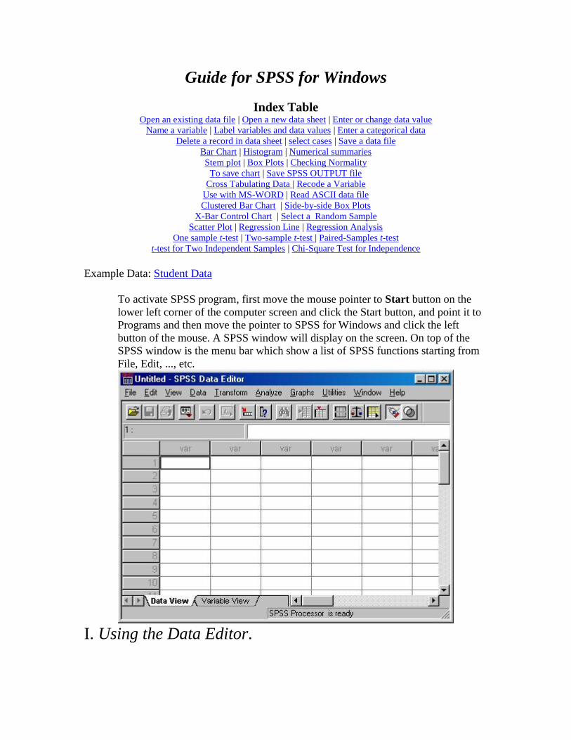
To activate SPSS program, first move the mouse pointer to Start button on the

lower left corner of the computer screen and click the Start button, and point it to

Programs and then move the pointer to SPSS for Windows and click the left

button of the mouse. A SPSS window will display on the screen. On top of the

SPSS window is the menu bar which show a list of SPSS functions starting from

File, Edit, ..., etc.

I. Using the Data Editor.

To open a new data file or a existing data file

Open an existing data file

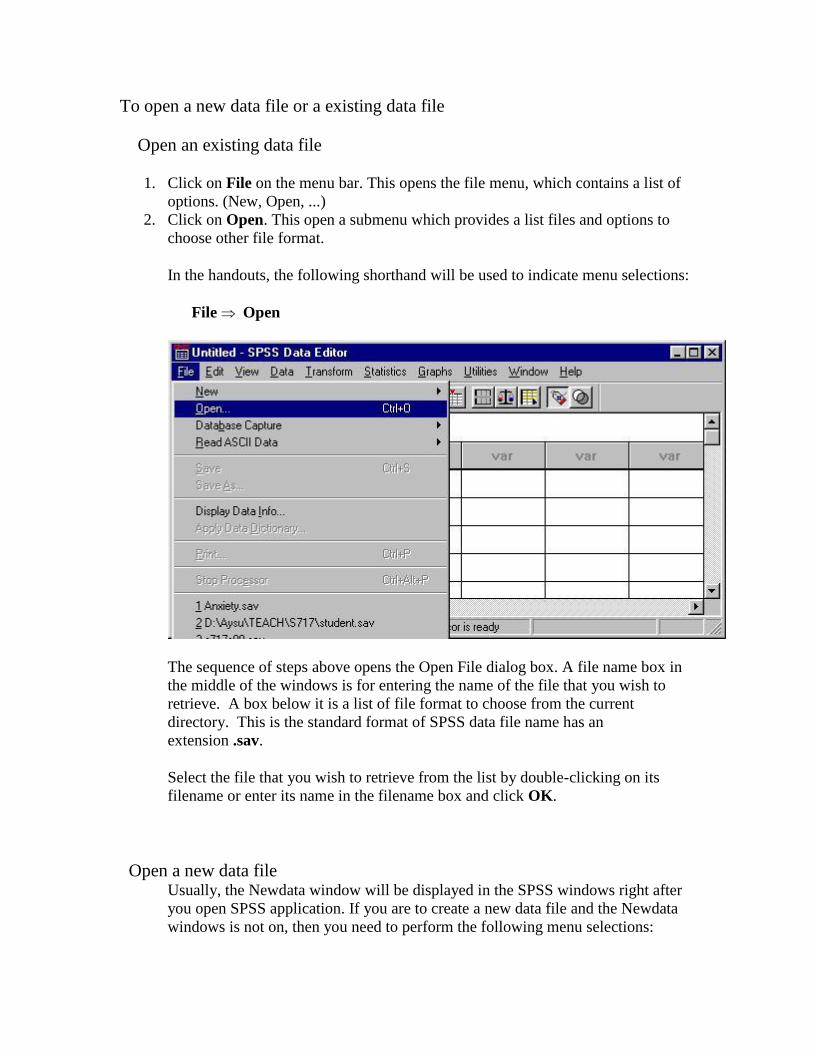
1. Click on File on the menu bar. This opens the file menu, which contains a list of

options. (New, Open, ...)

2. Click on Open. This open a submenu which provides a list files and options to

choose other file format.

In the handouts, the following shorthand will be used to indicate menu selections:

File Open

The sequence of steps above opens the Open File dialog box. A file name box in

the middle of the windows is for entering the name of the file that you wish to

retrieve. A box below it is a list of file format to choose from the current

directory. This is the standard format of SPSS data file name has an

extension .sav.

Select the file that you wish to retrieve from the list by double-clicking on its

filename or enter its name in the filename box and click OK.

Open a new data file

Usually, the Newdata window will be displayed in the SPSS windows right after

you open SPSS application. If you are to create a new data file and the Newdata

windows is not on, then you need to perform the following menu selections:

File New Data

and a Newdata window will appear in SPSS window for creating a new data file

(or data sheet).

SPSS 10.0 has a different user interface for data entering. SPSS 10.0 provides two views

in Data Editor. The variable can be entered using Data View and be defined in Variable

View. User can click the mouse on the Data View and Variable View labels of these two

views shown at the bottom of the editor to switch between the two views. To create a

new variable, user can double-click on "var" on top of the data column or click on

Variable View on the bottom of the Data Editor to bring up the Variable View and enter

variable name and type and other information.

To change or enter a piece of data in a data cell on the Data View sheet, just click on

the cell and type the data value and hit <enter>.

TRY IT Try entering the first three columns of the data in Student Data and

name the variables as they are defined in the handout. Each column contains data

for a variable. For recording data in integer format see the description in To

define a variable.

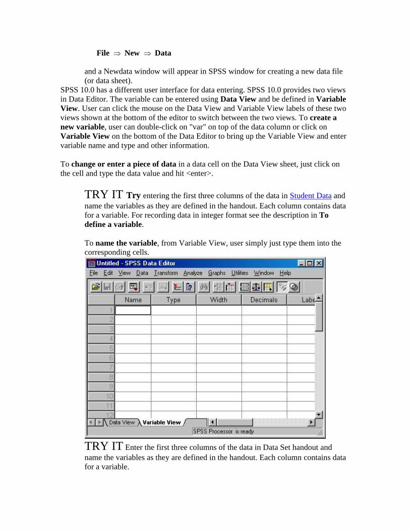
To name the variable, from Variable View, user simply just type them into the

corresponding cells.

TRY IT Enter the first three columns of the data in Data Set handout and

name the variables as they are defined in the handout. Each column contains data

for a variable.

To define or change variable type, labels or defining missing values, from

Variable View, just click on the corresponding cell and then click on a gray

button with three dots. A list of options or a dialog box will appear for user to

make changes.

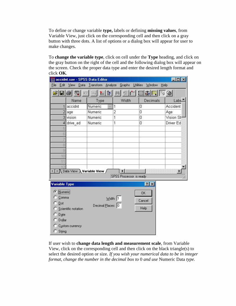
To change the variable type, click on cell under the Type heading, and click on

the gray button on the right of the cell and the following dialog box will appear on

the screen. Check the proper data type and enter the desired length format and

click OK.

If user wish to change data length and measurement scale, from Variable

View, click on the corresponding cell and then click on the black triangle(s) to

select the desired option or size. If you wish your numerical data to be in integer

format, change the number in the decimal box to 0 and use Numeric Data type.

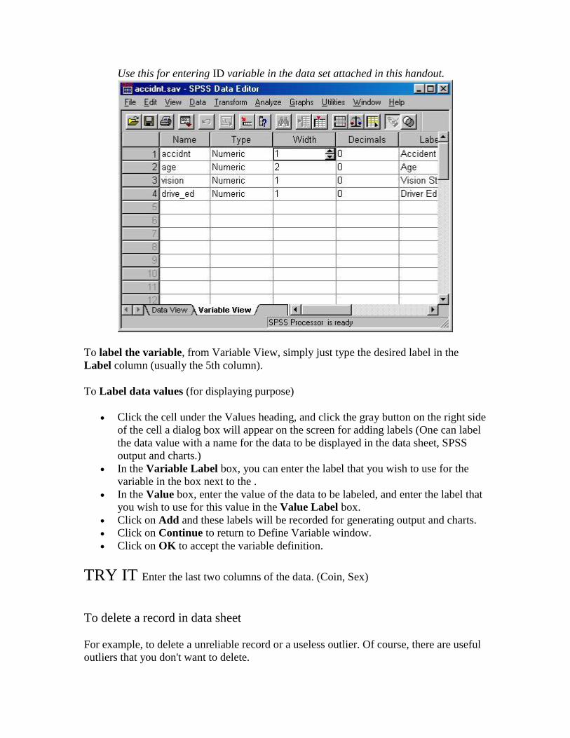
Use this for entering ID variable in the data set attached in this handout.

To label the variable, from Variable View, simply just type the desired label in the

Label column (usually the 5th column).

To Label data values (for displaying purpose)

Click the cell under the Values heading, and click the gray button on the right side

of the cell a dialog box will appear on the screen for adding labels (One can label

the data value with a name for the data to be displayed in the data sheet, SPSS

output and charts.)

In the Variable Label box, you can enter the label that you wish to use for the

variable in the box next to the .

In the Value box, enter the value of the data to be labeled, and enter the label that

you wish to use for this value in the Value Label box.

Click on Add and these labels will be recorded for generating output and charts.

Click on Continue to return to Define Variable window.

Click on OK to accept the variable definition.

TRY IT Enter the last two columns of the data. (Coin, Sex)

To delete a record in data sheet

For example, to delete a unreliable record or a useless outlier. Of course, there are useful

outliers that you don't want to delete.

Click on the number on the right end of the row of the data in the data sheet that you wish

to delete. Perform the following menu selections:

Edit Clear

The data record that you selected will disappear from the data sheet.

To enter a categorical data with numeric data type

Categorical data can be entered as numerical data and label them with labels. For

example, one can use "1" for "Male" and "0" for "Female" for entering data for SEX

variable. Labeling procedure described above can be used to label these data values with

their true meanings. Once the data values are labeled, you will see labels in stead of

numbers appear in data sheet while you're entering data with numbers. Make sure to

chick on View on the menu bar and check whether Value Labels item is checked or not.

If Value Labels is checked then the labels should be displayed on the screen instead of

their numerical values.

To select cases

1. Perform the following menu selections:

Data Select Cases

2. Select Cases dialog box will appear on the screen.

3. Choose a select option by clicking at the circle in front of the option. For

example, choose If condition is satisfied option and click on if... . Then, define

conditions in the Select Cases: if dialog box and click on continue and OK.

To clear the selection, click on All cases and click OK.

Select a Random Sample of Cases To select cases at random, first click on Data from the menu bar and then select

Select Cases and click on Random sample of cases and click

Sample ... . Specify the percentage or number cases to be sampled and continue

and OK the selection.

To save a data file

Make your Data Editor the active window.

Perform the following menu selections:

File Save As...

This open the Save Data window.

Enter a name for the data file in the File Name box and

option 1. (to save data in drive C:) click OK.

option 2. (to save data in drive A:) click on the down arrow symbol in the

Drives box and select A: drive and and enter the filename for the data

click OK. This will save the data file in the floppy disk that you put in

drive A. This data file will end with .sav. It indicates that the data is saved

in SPSS format.

Save the data to your disk in drive A: with the file name student.sav . This data file will

be used in the next section.

II. Generating Graphs and Summaries of Data(Output)

Exploratory Data Analysis

Stem and Leaf plot

The stem-and-leaf plot (or stemplot) is one of the tools in exploratory data analysis. To

construct a stemplot:

1. Perform the following menu selections:

Analyze Descriptive Statistics Explore...

The Explore window should then appear on the screen.

2. In Dependent list box, you can select a variable (height) for making stem plot.

Checking Normality & Making Histogram in Explore... Option

Click Analyze on the menu bar and selected Descriptive Statistics and select the

Explore option. After selection of variables, click on Plot option. One can check the

normality plots and tests and also check the Histogram option and click continue

to get back to the Explore dialog window and click on OK to execute the

procedure. A p-value (a value between 0 and 1) from K-S test for normality will be

produced for testing the normality of the data. A large p-value (usually large means

the p-value is greater than 0.05) indicates that the data follows a normal distribution

pattern.

*** The Explore… option is the best way of doing exploratory data analysis for quantitative

variable. The basic descriptive statistics, confidence interval estimate for mean, boxplot,

side-by-side boxplot, normality test and plot, histogram, and stemplot can all be

produced from this option.

*** For describing categorical variable, one should click through:

Analyze->Descriptive Statistics->Frequencies…

to obtain frequency distribution table and making bar chart or pie chart in this option.

Bar Chart Try the following menu selections,

Graphs Bar...

Select a chart type (try Simple) you prefer and click on Define.

A Define Simple Bar box will appear. Try selecting the variable sex into Categorical

Axis and click on OK.

Try to make a pie-chart using the Pie... option.

To save chart

You can save charts by at least the following two ways:

1. Save a chart by copying chart and pasting it to new empty OUTPUT file.

2. Export the chart to any of the several common formats, (such as .gif .jpg .bmp ...),

by performing the following menu selections

File Export ...

and in the Export box, select chart only, and in the File Prefix box enter the chart

filename and path, and in the File Type box, select the desired format.

Clustered Bar Chart

Let's try to create a clustered bar chart using the data file student. Use the Open Existing

Data File procedure you've learned in last handout to open employee data file.

[1] First, perform the following menu selections:

Graphs Bar... [2] The Bar Chart box should appear on the screen.

[3] Click on Clustered and select Summaries for groups of cases and click Define. The

Define Clustered Bar window should appear.

[4] Use % of cases in Bars Represent box and

[5] select sex for Categories Axis and

[6] select coin for Define Clusters by and click OK.

Repeat the same steps above and change the last three steps to the followings:

Try to use N of cases in Bars Represent box and

select sex for Categories Axis and

select coin for Define Clusters by and click OK.

Histogram Try the following menu selections,

Graphs Histogram

A Histogram box will appear. Select the variable to be displayed and OK it.

Double click on any part of the chart will activate the chart editing window and allow you

to modify the chart.

To modify number of intervals in a histogram, in the chart editing windows use the

following menu selections

Chart Axis Interval Custom Define

and change the number of intervals, and click on continue or OK to close all the dialog

boxes for modifying chart in the chart editing window.

Normality Test in Nonparametric Tests Option To find the p-value of the K-S Lilliefors test, click Analyze and select

Nonparametric Tests and then 1-Sample K-S) in the OUTPUT window. The p-

value is the value under “Sig.” in the table. A large p-value, generally greater than

0.05, indicates that the data is likely normally distributed.

To obtain some numerical summaries (Try studentp.sav data file.)

Perform the following menu selections:

Analyze Descriptive Statistics Descriptives ...

a Descriptives box will appear, and select variables height, (or weight) and then click

OK. In the output window, you will see some descriptive statistics for these selected

variables.

To save SPSS OUTPUT file

Save OUTPUT file in drive A by 1) clicking File and 2) select Save As, 3) select a disk

drive to save file, and then 4) enter the name of the file you want it to be. The file will

end with .spo. You can modify the OUTPUT file by clicking the mouse at the place

where you wish to add or delete graph or tables.

Box Plots ( Try studentp.sav data file.)

To generate a bloxplot for one variable (weight):

1. perform the following menu selections:

Graphs Boxplot

2. The Boxplot window should then appear on the screen.

3. Select simple boxplot option.

4. Check on summaries of separate variables and click Define, and a Simple Boxplot

Window should appear.

5. Select weight as the boxes represents variable and click OK.

This will generate a box plot to describe the distribution of weight variable. The outliers

will be labeled if specified in the Define Simple Boxplot Window.

In the OUTPUT window, you should also see the stem-and-leaf diagrams displaying

distributions of weight. This is because the stem plot option is always checked in the

boxplot menu unless you change it to not making stem plot.

Side-by-side Box Plots ( Try studentp.sav data file.)

To perform exploratory data analysis by viewing stem-and-leaf charts and box plots:

1. Perform the following menu selections:

Analyze Descriptive Explore...

The Explore window should then appear on the screen.

2. For Dependent list box select weight.

3. For Factor list box select sex.

4. For Label cases by: select id.

This will generate two box plots, one for male and one for female to describe the

distribution of weight variable. The outliers will be labeled by their ID. One can generate

a box plot for one variable by not selecting any variable for Factor list. In the OUTPUT

window, you should also see the stem plot displaying distributions of weight for male and

female.

Can you make a boxplot for the weight from only female students ????

X-Bar Control Chart To make a X-Bar Chart, first enter data with one subgroup variable and several

sample variables, then perform the following menu selections:

Graphs Select Control ...

(The control chart dialog box will appear.)

1. Select Cases are subgroups and select X-bar chart and click Define

2. In the control chart box enter the subgroup variable and also enter sample

variables into the samples box and select other options if needed.

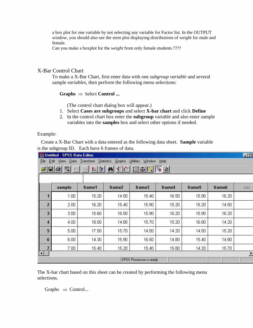
Example:

Create a X-Bar Chart with a data entered as the following data sheet. Sample variable

is the subgroup ID. Each have 6 frames of data.

The X-bar chart based on this sheet can be created by performing the following menu

selections.

Graphs Control...

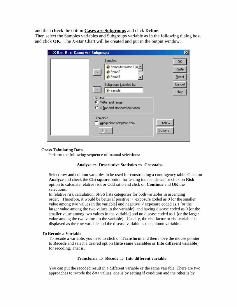
and then check the option Cases are Subgroups and click Define.

Then select the Samples variables and Subgroups variable as in the following dialog box.

and click OK. The X-Bar Chart will be created and put in the output window.

Cross Tabulating Data

Perform the following sequence of manual selections:

Analyze Descriptive Statistics Crosstabs...

Select row and column variables to be used for constructing a contingency table. Click on

Analyze and check the Chi-square option for testing independence, or click on Risk

option to calculate relative risk or Odd ratio and click on Continue and OK the

selections.

In relative risk calculation, SPSS lists categories for both variables in ascending

order. Therefore, it would be better if positive '+' exposure coded as 0 [or the smaller

value among two values in the variable] and negative '-' exposure coded as 1 [or the

larger value among the two values in the variable], and having disease coded as 0 [or the

smaller value among two values in the variable] and no disease coded as 1 [or the larger

value among the two values in the variable]. Usually, the risk factor or risk variable is

displayed as the row variable and the disease variable is the column variable.

To Recode a Variable

To recode a variable, you need to click on Transform and then move the mouse pointer

to Recode and select a desired option (Into same variables or Into different variable)

for recoding. That is,

Transform Recode Into different variable

You can put the recoded result in a different variable or the same variable. There are two

approaches to recode the data values, one is by setting if condition and the other is by

specifying Old and New values. To recode data values and store in a new variable, in the

Recode in Different Variables window:

1. First select (double click) a variable to be recoded and then enter the name for the new

variable to store the new codes (the box on top right hand corner) and click on Change.

You should see old-variable - new-variable appear in the big box.

2. If the Old and New values option is selected, a dialog box will appear on the screen.

i. Specify the value or the range of values to be recoded by clicking the

circle in front of the option and entering value or range within the New

value box.

ii. Enter the new value into the box in the Old value box and click on Add

to define this transformation.

iii. Continue the first two steps (i, ii) for defining transformation of data

values in other ranges and click on Continue.

Click on OK to complete the recoding.

Use a word processor (Microsoft Word) to produce a statistical report

Open the word processor Microsoft WORD.

You can copy pictures or tables generated by SPSS to a word processor. For copying

charts or tables you need to:

1. activate the Chart Editor (by double-click on chart) or click on table and then

click on Edit and select Copy or Copy objects, and the chart or table will be

kept in the clipboard, (Copy objects is a prefer option, since it produce better

results.)

2. then activate the word processor and click on the location that you wish to

paste the chart or table, and select Edit and then select Paste to paste the

chart or table to your report.

Remark: Use the chart editing window to modify you chart if necessary, and then past it

to your MS-WORD. This will improve the quality of the chart in the MS-WORD. You

can also adjust the size of the chart in MS-WORD.

III. How to read ASCII data file

1. Perform the following sequence of menu selections

File Read ASCII Data ...

2. Select Freefield, if you don't want a special input format for read in data.

3. Click on Browse... for getting ascii file that you wish to read into the data editor.

Note:

o The data file need to be checked first to see whether it is ready to be read

into the SPSS data editor. If it is not ready, one may have to use a word

processor to modify it so that it can be read into the data editor.

o Data are considered to be separated by space when Freefield is used.

4. Name the variables according to the order of the data values to be read, define the

variable type, click Add to add variable name one at a time, and click on OK

when all the variables are defined.

IV. Examine relationship between two quantitative

variables

Scatter Plot 1. Perform the following sequence of menu selections

Graphs Scatter...

2. Select a variable of Y axis and select a variable of X axis.

3. Click OK.

Draw a Regression Line

1. To draw a regression line to fit the data points, first double click on any part of the

chart (the scatter plot) to bring up the chart editor, then do the following sequence

of menu selections

Chart Options ...

2. In the Scatterplot Options box check on the proper Fit line options.

** Click on button in Chart Editor window, the mouse pointer on the screen will

change shape and click of the dot on the scatter plot for displaying case number for the

data.

Regression Analysis

1. Perform the following sequence of menu selections

Analyze Regression Linear ...

2. Select the dependent variable (response variable) and independent variables

(explanatory variables, or predictor variables)

3. Residual plots can be produced through plot option and residual can be save

through save option.

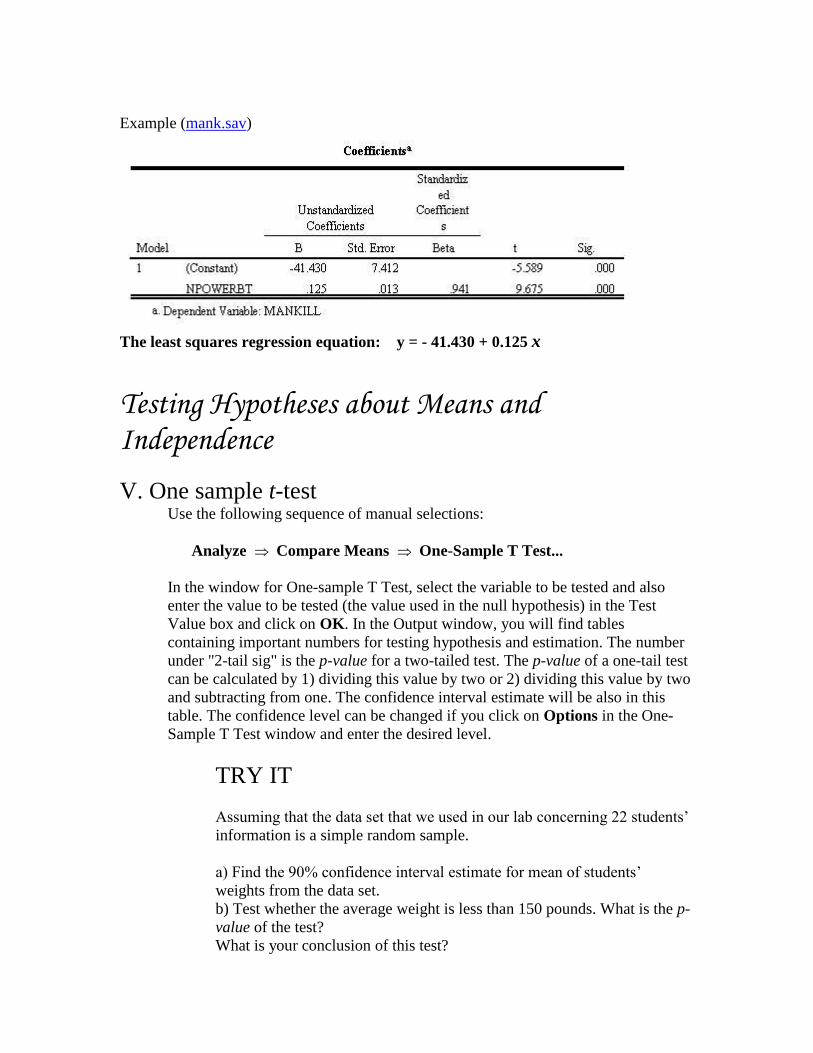
Example (mank.sav)

The least squares regression equation: y = - 41.430 + 0.125 x

Testing Hypotheses about Means and Independence

V. One sample t-test

Use the following sequence of manual selections:

Analyze Compare Means One-Sample T Test...

In the window for One-sample T Test, select the variable to be tested and also

enter the value to be tested (the value used in the null hypothesis) in the Test

Value box and click on OK. In the Output window, you will find tables

containing important numbers for testing hypothesis and estimation. The number

under "2-tail sig" is the p-value for a two-tailed test. The p-value of a one-tail test

can be calculated by 1) dividing this value by two or 2) dividing this value by two

and subtracting from one. The confidence interval estimate will be also in this

table. The confidence level can be changed if you click on Options in the One-

Sample T Test window and enter the desired level.

TRY IT

Assuming that the data set that we used in our lab concerning 22 students’

information is a simple random sample.

a) Find the 90% confidence interval estimate for mean of students’

weights from the data set.

b) Test whether the average weight is less than 150 pounds. What is the p-

value of the test?

What is your conclusion of this test?

VI. Two-sample t-test

Paired-Samples t-test

Use the following sequence of manual selections:

Analyze Compare Means Paired-Samples T Test...

In the Paired-sample T Test window, select two variables to be tested by simply

clicking on these variables and click on OK. In the Output window, you will find

tables containing important numbers for testing hypothesis and estimation. The

number under "2-tail sig" is the p-value for a two-tailed test. The p-value of a one-

tail test can be calculated by 1) dividing this value by two or 2) dividing this value

by two and subtracting from one. The confidence interval estimate will be also in

this table. The confidence level can be changed if you click on Options in the

Paired-Samples T Test window and enter the desired level.

TRY IT

Assuming that the data set from employee data file is just a random

sample.

a) Find the 90% confidence interval estimate for the mean of differences

of beginning (salbeg) and present (salary) salary from the employee data.

b) Test whether the beginning salary (salbeg) is lower than the salary now

(salary). What is the p-value of the test?

t-test for Two Independent Samples

Use the following sequence of manual selections:

Analyze Compare Means Independent-Samples T Test...

In the window for Independent-samples T Test, 1) select the variable to be tested

and also 2) select the grouping variable to be used to identify groups in the test

and 3) define the two groups to be tested by clicking the Define Groups and 4)

enter values that represent different group in the grouping variable (for example,

select salbeg as test variable and select gender as grouping variable, and click

Define Groups and then enter 0 and 1 in the Define Groups window for indicating

female and male groups) and click on OK. In the Output window, you will find

tables containing important numbers for testing hypothesis and estimation. The

number under "2-tail sig" is the p-value for a two-tailed test. Depending on the

alternative hypothesis of the test, the p-value of a one-tail test can be calculated

by 1) dividing this value by two or 2) dividing this value by two and then

subtracting from one. There are two p-values of the test in the "t-test for Equality

of Means" table for equal and unequal variance conditions. The result of an F-test

for equality of variances in the output window above this table can help us to

determine which p-value is the proper one to use.

The confidence interval estimate will be also in this table. The confidence level

can be changed if you click on Options in the Independent-samples T Test

window and enter the desired level.

TRY IT

Assuming that the data set from students’ information is just a random

sample.

a) Find the 90% confidence interval estimate for the difference of average

weights for male and female students.

b) Test whether there is a difference between the average weights for male

and female students.

What is your conclusion?

VII. Chi-Square Test for Independence

Use the following sequence of manual selections:

Analyze Descriptive Statistics Crosstabs...

Select row and column variables to be used for constructing a contingency table

and click on Analyze and check the chi-square option and OK the selections.