1. INTRODUCTIONAfter years of relative neglect in academic circles, portfolio choice problems are again atthe forefront of financial research. The economic theory underlying an investor’s opti-mal portfolio choice, pioneered by Markowitz (1952), Merton (1969, 1971), Samuelson(1969), and Fama (1970), is by now well understood. The renewed interest in port-folio choice problems follows the relatively recent empirical evidence of time-varyingreturn distributions (e.g., predictability and conditional heteroskedasticity) and is fueledby realistic issues including model and parameter uncertainty, learning, background risks,and frictions. The general focus of the current academic research is to identify keyaspects of real-world portfolio choice problems and to understand qualitatively as well asquantitatively their role in the optimal investment decisions of individuals and institutions.
Whether for academic researchers studying the portfolio choice implications of returnpredictability, for example,or for practitioners whose livelihood depends on the outcomeof their investment decisions, a critical step in solving realistic portfolio choice problemsis to relate the theoretical formulation of the problem and its solution to the data.Thereare a number of ways to accomplish this task, ranging from calibration with only vagueregard for the data to decision theoretic approaches which explicitly incorporate thespecification of the return model and the associated statistical inferences in the investor’sdecision process. Surprisingly, given the practical importance of portfolio choice prob-lems, no single econometric approach has emerged yet as clear favorite. Because eachapproach has its advantages and disadvantages, an approach favored in one context isoften less attractive in another.
This chapter is devoted to the econometric treatment of portfolio choice problems.The goal is to describe,discuss, and illustrate through examples the different econometricapproaches proposed in the literature for relating the theoretical formulation and solutionof a portfolio choice problem to the data.The chapter is intended for academic researcherswho seek an introduction to the empirical implementation of portfolio choice problemsas well as for practitioners as a review of the academic literature on the topic. In focusingon the econometrics of the portfolio choice problem, this chapter is at best a cursoryoverview of the broad portfolio choice literature. In particular, much of the discussionis focused on the single period portfolio choice problem with standard preferences,normally distributed returns, and frictionless markets.There are many recent advances inthe portfolio choice literature, some cited below but many regrettably omitted, that relaxone or more of these simplifying assumptions.The econometric techniques discussed inthis chapter can be applied to these more realistic formulations.
The chapter is divided into three parts. Section 2 reviews the theory of portfoliochoice in discrete and continuous time. It also discusses a number of modeling issues andextensions that arise in formulating the problem. Section 3 presents the two traditionaleconometric approaches to portfolio choice problems: plug-in estimation and Bayesian
Portfolio Choice Problems 271
decision theory. In Section 4, I then describe a more recently developed econometricapproach for drawing inferences about optimal portfolio weights without modelingreturn distributions.
2. THEORETICAL PROBLEM2.1. Markowitz Paradigm
The mean–variance paradigm of Markowitz (1952) is by far the most common for-mulation of portfolio choice problems. Consider N risky assets with random returnvector Rt+1 and a riskfree asset with known return Rf
t . Define the excess returnsrt+1 = Rt+1 − Rf
t and denote their conditional means (or risk premia) and covariancematrix by μt and #t , respectively. Assume, for now, that the excess returns are i.i.d. withconstant moments.
Suppose the investor can only allocate wealth to the N risky securities. In the absenceof a risk-free asset, the mean–variance problem is to choose the vector of portfolioweights x, which represent the investor’s relative allocations of wealth to each of the Nrisky assets, to minimize the variance of the resulting portfolio return Rp,t+1 = x′Rt+1
for a predetermined target expected return of the portfolio Rft + μ:
minx
var[Rp,t+1] = x′#x, (2.1)
subject to
E[Rp,t+1] = x′(Rf + μ) = (Rf + μ) andN∑
i=1
xi = 1. (2.2)
The first constraint fixes the expected return of the portfolio to its target, and the sec-ond constraint ensures that all wealth is invested in the risky assets. Setting up theLagrangian and solving the corresponding first-order conditions (FOCs), the optimalportfolio weights are as follows:
x* = +1 ++2μ (2.3)
with
+1 = 1D
[B(#−1ι)− A(#−1μ)
]and +2 = 1
D
[C(#−1μ)− A(#−1ι)
], (2.4)
where ι denotes an appropriately sized vector of ones and where A = ι′#−1μ, B =μ′#−1μ,C = ι′#−1ι, and D = BC − A2.The minimized portfolio variance is equal tox*′#x*.
The Markowitz paradigm yields two important economic insights. First, it illustratesthe effect of diversification. Imperfectly correlated assets can be combined into portfolios
Mean–varianceefficient frontier with risk-free rate
o
o
o
10 industry portfolios
Figure 5.1 Mean–variance frontierswith andwithout risk-free asset generatedbyhistoricalmomentsof monthly returns on 10 industry-sorted portfolios. Expected return and volatility are annualized.
with preferred expected return-risk characteristics. Second, the Markowitz paradigmshows that, once a portfolio is fully diversified, higher expected returns can only beachieved through more extreme allocations (notice x* is linear in μ) and therefore bytaking on more risk.
Figure 5.1 illustrates graphically these two economic insights. The figure plots ashyperbola the mean–variance frontier generated by the historical moments of monthlyreturns on 10 industry-sorted portfolios. Each point on the frontier gives along thehorizonal axis the minimized portfolio return volatility (annualized) for a predeterminedexpected portfolio return (also annualized) along the vertical axis. The dots inside thehyperbola represent the 10 individual industry portfolios from which the frontier isconstructed. The fact that these dots lie well inside the frontier illustrates the effect ofdiversification. The individual industry portfolios can be combined to generate returnswith the same or lower volatility and the same or higher expected return. The figurealso illustrates the fundamental trade-off between expected return and risk. Starting withthe least volatile portfolio at the left tip of the hyperbola (the global minimum varianceportfolio), higher expected returns can only be achieved at the cost of greater volatility.
If the investor can also allocate wealth to the risk-free asset, in the form of unlimitedrisk-free borrowing and lending at the risk-free rate Rf
t , any portfolio on the mean–variance frontier generated by the risky assets (the hyperbola) can be combined with therisk-free asset on the vertical axis to generate an expected return-risk profile that lies on astraight line from the risk-free rate (no risky investments) through the frontier portfolio
Portfolio Choice Problems 273
(fully invested in risky asset) and beyond (leveraged risky investments). The optimalcombination of the risky frontier portfolios with risk-free borrowing and lendingis the one that maximizes the Sharpe ratio of the overall portfolio, defined asE[rp,t+1]/std[rp,t+1] and represented graphically by the slope of the line from the risk-freeasset through the risky frontier portfolio.The highest obtainable Sharpe ratio is achievedby the upper tangency on the hyperbola shown in Fig. 5.1. This tangency thereforerepresents the mean–variance frontier with risk-free borrowing and lending.The criticalfeature of this mean–variance frontier with risk-free borrowing and lending is that everyinvestor combines the risk-free asset with the same portfolio of risky assets – the tangencyportfolio in Fig. 5.1.
In the presence of a risk-free asset, the investor allocates fractions x of wealth to therisky assets and the remainder (1− ι′x) to the risk-free asset.The portfolio return is there-fore Rp,t+1 = x′Rt+1 + (1− ι′x)Rf
t = x′rt+1 + Rft and the mean–variance problem can
be expressed in terms of excess returns:
minx
var[rp] = x′#x subject to E[rp] = x′μ = μ. (2.5)
The solution to this problem is much simpler than in the case without a risk-free asset:
x* = μ
μ′#−1μ︸ ︷︷ ︸λ
×#−1μ, (2.6)
where λ is a constant that scales proportionately all elements of #−1μ to achieve thedesired portfolio risk premium μ. From this expression, the weights of the tangencyportfolio can be found simply by noting that the weights of the tangency portfolio mustsum to one, because it lies on the mean–variance frontier of the risky assets. For thetangency portfolio:
λtgc = 1ι′#−1μ
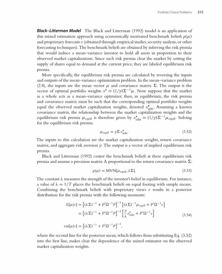
and μtgc =μ′#−1μ
ι′#−1μ. (2.7)
The formulations (2.1) and (2.2) or (2.5) of the mean–variance problem generate amapping from a predetermined portfolio risk premium μ to the minimum–varianceportfolio weights x* and resulting portfolio return volatility
√x*′#x*. The choice of
the desired risk premium, however, depends inherently on the investor’s tolerance forrisk. To incorporate the investor’s optimal trade-off between expected return and risk,the mean–variance problem can be formulated alternatively as the following expectedutility maximization:
maxx
E[rp,t+1] − γ
2var[rp,t+1], (2.8)
274 Michael W. Brandt
where γ measures the investor’s level of relative risk aversion. The solution to thismaximization problem is given by Eq. (2.6) with λ = 1/γ , which explicitly links theoptimal allocation to the tangency portfolio to the investor’s tolerance for risk.
The obvious appeal of the Markowitz paradigm is that it captures the two fundamentalaspects of portfolio choice – diversification and the trade-off between expected returnand risk – in an analytically tractable and easily extendable framework. This has made itthe de-facto standard in the finance profession. Nevertheless, there are several commonobjections to the Markowitz paradigm. First, the mean–variance problem only representsan expected utility maximization for the special case of quadratic utility, which is aproblematic preference specification because it is not monotonically increasing in wealth.For all other utility functions, the mean–variance problem can at best be interpreted as asecond-order approximation of expected utility maximization. Second, but related, themean–variance problem ignores any preferences toward higher-order return moments, inparticular toward return skewness and kurtosis. In the context of interpreting the mean–variance problem as a second-order approximation, the third and higher-order termsmay be economically nonnegligible. Third, the mean–variance problem is inherentlya myopic single-period problem, whereas we think of most investment problems asinvolving longer horizons with intermediate portfolio rebalancing. Each criticism hasprompted numerous extensions of the mean–variance paradigm.1 However, the moststraightforward way to address all these issues, and particularly the third, is to formulatethe problem explicitly as an intertemporal expected utility maximization.
2.2. Intertemporal Expected Utility Maximization2.2.1. Discrete Time Formulation
Consider the portfolio choice at time t of an investor who maximizes the expected utilityof wealth at some future date t + τ by trading in N risky assets and a risk-free asset attimes t, t + 1, . . . , t + τ − 1. The investor’s problem is
V (τ, Wt , zt) = max{xs}t+τ−1
s=t
Et[u(Wt+τ)
], (2.9)
subject to the budget constraint:
Ws+1 = Ws(xs′rs+1 + Rf
s)
(2.10)
and having positive wealth each period,Ws ≥ 0.The function u(·)measures the investor’sutility of terminal wealth Wt+τ , and the subscript on the expectation denotes that
1The majority of extensions deal with incorporating higher-order moments. For example, in Brandt et al. (2005), we propose a fourth-order approximation of expected utility maximization that captures preferences toward skewness and kurtosis.While the optimal portfolioweights cannot be solved for analytically, we provide a simple and efficient numerical procedure. Other work on incorporating higher-order moments include Kraus and Litzenberger (1976), Kane (1982), Simaan (1993), de Athayde and Flores (2004), and Harvey et al.(2004).
Portfolio Choice Problems 275
the expectation is taken conditional on the information set zt available at time t.For concreteness, think of zt as a K <∞ dimensional vector of state variables andassume that yt ≡ [rt , zt] evolves as a first-order Markov process with transition densityf (yt |yt−1).2
The case τ = 1 corresponds to a static single-period optimization. In general,however,the portfolio choice is a more complicated dynamic multiperiod problem. In choosing atdate t the optimal portfolio weights xt conditional on having wealth Wt and informationzt , the investor takes into account that at every future date s the portfolio weights willbe optimally revised conditional on the then available wealth Ws and information zs.
The function V (τ, Wt , zt) denotes the investor’s expectation at time t, conditionalon the information zt , of the utility of terminal wealth Wt+τ generated by the currentwealth Wt and the sequence of optimal portfolio weights {x*s }t+τ−1
s=t over the next τperiods. V (·) is called the value function because it represents the value, in units ofexpected utils,of the portfolio choice problem to the investor.Think of the value functionas measuring the quality of the investment opportunities available to the investor. Ifthe current information suggests that investment opportunities are good, meaning, forexample, that the sequence of optimal portfolio choices is expected to generate an aboveaverage return with below average risk, the current value of the portfolio choice problemto the investor is high. If investment opportunities are poor, the value of the problemis low.
The dynamic nature of the multiperiod portfolio choice is best illustrated byexpressing the problem (2.9) as a single-period problem with state-dependent utilityV (τ − 1, Wt+1, zt+1) of next period’s wealth Wt+1 and information zt+1:
V (τ, Wt , zt) = max{xs}t+τ−1
s=t
Et[u(Wt+τ
)]= max
xtEt
[max
{xs}t+τ−1s=t+1
Et+1[u(Wt+τ
)]](2.11)
= maxxt
Et[V(τ − 1, Wt
(xt′rt+1 + Rf
t), zt+1
)],
subject to the terminal condition V (0, Wt+τ , zt+τ) = u(Wt+τ). The second equalityfollows from the law of iterated expectations and the principle of optimality. The thirdequality uses the definition of the value function as well as the budget constraint. Itis important to recognize that the expectation in the third line is taken over the jointdistribution of next period’s returns rt+1 and information zt+1,conditional on the currentinformation zt .
2The first-order assumption is innocuous because zt can contain lagged values.
276 Michael W. Brandt
Equation (2.11) is the so-called Bellman equation and is the basis for any recursivesolution of the dynamic portfolio choice problem. The FOCs for an optimum at eachdate t are3
Et
[V2
(τ − 1, Wt
(xt′rt+1 + Rf
t), zt+1
)rt+1
]= 0, (2.12)
where Vi(·) denotes the partial derivative with respect to the ith argument of the valuefunction.These FOCs make up a system of nonlinear equations involving possibly high-order integrals and can in general be solved for xt only numerically.
CRRA Utility Example For illustrative purposes, consider the case of constant rela-tive risk aversion (CRRA) utility u(Wt+τ) = Wt+τ1−γ/(1− γ), where γ denotes thecoefficient of relative risk aversion. The Bellman equation then simplifies to:
V (τ, Wt , zt) = maxxt
Et
[max
{xs}t+τ−1s=t+1
Et+1
[Wt+τ1−γ
1− γ
]]
= maxxt
Et
[max
{xs}t+τ−1s=t+1
Et+1
[(Wt
∏t+τ−1s=t
(xs′rs+1 + Rf
s))1−γ
1− γ
]](2.13)
= maxxt
Et
[ (Wt
(xt′rt+1+ Rf
t))1−γ
1− γ︸ ︷︷ ︸u(Wt+1
)max
{xs}t+τ−1s=t+1
Et+1
[(∏t+τ−1s=t+1
(xs′rs+1 + Rf
s))1−γ]
︸ ︷︷ ︸ψ(τ − 1, zt+1)
]
In words, with CRRA utility the value function next period, V (τ − 1, Wt+1, zt+1), isequal to the product of the utility of wealth u(Wt+1) and a function ψ(τ − 1, zt+1)
of the horizon τ − 1 and the state variables zt . Furthermore, as the utility function ishomothetic in wealth we can, without loss of generality, normalize Wt = 1. It followsthat the value function depends only on the horizon and state variables, and that theBellman equation is
11− γ
ψ(τ, zt) = maxxt
Et
[(xt′rt+1 + Rf
t)1−γ
1− γψ(τ − 1, zt+1
)]. (2.14)
The corresponding FOCs are
Et
[(xt′rt+1 + Rf
t)−γ
ψ(τ − 1, zt+1
)rt+1
]= 0, (2.15)
which,despite being simpler than in the general case, can still only be solved numerically.
3As long as the utility function is concave, the second-order conditions are satisfied.
Portfolio Choice Problems 277
The Bellman equation for CRRA utility illustrates how the dynamic and myopicportfolio choices can differ. If the excess returns rt+1 are contemporaneously independentof the innovations to the state variables zt+1, the optimal τ and one-period portfoliochoices at date t are identical because the conditional expectation in the Bellman equationfactors into a product of two conditional expectations. The first expectation is of theutility of next period’s wealth u(Wt+1), and the second is of the function of the statevariablesψ(τ − 1, zt+1). Because the latter expectation does not depend on the portfolioweights, the FOCs of the multiperiod problem are the same as those of the single-periodproblem. If, in contrast, the excess returns are not independent of the innovations tothe state variables, the conditional expectation does not factor, the FOCs are not thesame, and, as a result, the dynamic portfolio choice may be substantially different fromthe myopic portfolio choice.The differences between the two policies are called hedgingdemands because by deviating from the single-period portfolio choice the investor triesto hedge against changes in the investment opportunities.
More concretely,consider as data generating process f (yt |yt−1) the following restrictedand homoscedastic vector auto-regression (VAR) for the excess market return anddividend yield (in logs):4 [
ln(1+ rt+1)
ln dpt+1
]= β0 + β1 ln dpt + εt+1, (2.16)
where dpt+1 denotes the dividend-to-price ratio and εt+1i.i.d.∼ MVN[0,#]. Table 5.1
presents ordinary least squares (OLS) estimates of this return model for quarterly realdata on the value weighted CRSP index and 90-day Treasury bill rates from April 1952
Table 5.1 OLS estimates of the VAR using quarterly real data on the value weightedCRSP index and 90-day Treasury bill rates from April 1952 through December 1996
4This data generating process is motivated by the evidence of return predictability by the dividend yield (e.g., Campbell and Shiller, 1988;Fama and French, 1988) and has been used extensively in the portfolio choice literature (e.g., Barberis, 2000; Campbell and Viceira, 1999;Kandel and Stambaugh, 1996).
278 Michael W. Brandt
through December 1996.5 The equation-by-equation adjusted R2s are 2.3 and 89.3%,reflecting the facts that is it quite difficult to forecast excess returns and that the dividendyield is highly persistent and predictable.
Taking these estimates of the data generating process as the truth, the FOCs (2.15) canbe solved numerically using a variety of dynamic programming methods (see Judd,1998,for a review of numerical methods for dynamic programming). Figure 5.2 presents thesolution to the single-period (one-quarter) problem. Plot A shows the optimal fractionof wealth invested in stocks x*t as a function of the dividend yield. Plot B shows thecorresponding annualized certainty equivalent rate of return Rce
t (τ), defined as the risk-free rate that makes the investor indifferent between holding the optimal portfolio andearning the certainty equivalent rate over the next τ periods.6 The solid, dashed-dotted,and dotted lines are for relative risk aversion γ of 2, 5, and 10, respectively.
At least three features of the solution to the single-period problem are noteworthy.First, both the optimal allocation to stocks and the certainty equivalent rate increasewith the dividend yield, which is consistent with the fact that the equity risk premiumincreases with the dividend yield. Second, the extent to which the investor tries totime the market decreases with risk aversion. The intuition is simple. When the riskpremium increases, stocks become more attractive (higher expected return for the same
2.0 3.0 4.0 5.0 6.00
0.2
0.4
0.6
0.8
1.0Plot A
2.0 3.0 4.0 5.0 6.00
5.0
10.0
15.0
20.0
25.0Plot B
Figure 5.2 Plot A shows the optimal fraction ofwealth invested in stocks as a function of the dividendyield for a CRRA investor with one-quarter horizon and relative risk aversion of 2 (solid line), 5 (dashed-dotted line), and 10 (dotted line). Plot B shows the corresponding annualize certainty equivalent ratesof return (in percent).
5Note that the evidence of return predictability by the dividend yield has significantly weakened over the past 7 years (1997–2003) (e.g.,Ang and Bekaert, 2007; Goyal and Welch, 2003). I ignore this most recent sample period for illustrative purposes and to reflect theliterature on portfolio choice under return predictability by the dividend yield (e.g., Barberis, 2000; Campbell and Viceira, 1999; Kandeland Stambaugh, 1996). However, keep in mind that the results do not necessarily reflect the current data.
6For CRRA utility, the certainty equivalent rate is defined by[Rce
t (τ)Wt]1−γ
/(1− γ) = V (τ, Wt , zt ).
Portfolio Choice Problems 279
level of risk), and consequently the investor allocates more wealth to stocks. As thestock allocation increases, the mean of the portfolio return increases linearly while thevariance increases quadratically and hence at some point increases faster than the mean.Ignoring higher-order moments, the optimal allocation sets the expected utility gainfrom a marginal increase in the portfolio mean to equal the expected utility loss from theassociated increase in the portfolio variance.The willingness to trade off expected returnfor risk at the margin depends on the investor’s risk aversion. Third, the benefits frommarket timing also decrease with risk aversion.This is because a more risk averse investorallocates less wealth to stocks and therefore has a lower expected portfolio return andbecause, even for the same expected portfolio return, a more risk averse investor requiresa smaller incentive to abstain from risky investments.
Figure 5.3 presents the solution to the multiperiod portfolio choice for horizons τranging from one quarter to 10 years for an investor with γ = 5 (corresponding to thedashed-dotted lines in Fig. 5.2). Rather than plotting the entire policy fuction for eachhorizon, plot A shows only the allocations for current dividend yields of 2.9% (25th per-centile, dotted line), 3.5% (median, dashed-dotted line), and 4.1% (75th percentile, solidline). Plot B shows the expected utility gain, measured by the increase in the annualizedcertainty equivalent rates (in percent), from implementing the dynamic multiperiod port-folio policy as opposed to making a sequence of myopic single-period portfolio choices.
It is clear from plot A that the optimal portfolio choice depends on the investor’shorizon. At the median dividend yield, for example, the optimal allocation is 58% stocksfor a one-quarter horizon (one period), 66% stocks for a 1-year horizon (four periods),
0 1 2 3 4 5 6 7 8 9 100
0.1
0.2
0.3
0.4
0.5
0.6Plot B
0 1 2 3 4 5 6 7 8 9 100
0.2
0.4
0.6
0.8
1.0Plot A
Figure 5.3 Plot A shows the optimal fraction of wealth invested in stocks as a function of theinvestment horizon for a CRRA investor with relative risk aversion of five conditional on the currentdividend yield being equal to 2.9 (dotted line), 3.5 (dashed-dotted line), and 4.1 (solid line) percent.Plot B shows the corresponding increase in the annualized certainty equivalent rates of return frominvesting optimally as opposed to myopically (in percent).
280 Michael W. Brandt
96% stocks for a 5-year horizon (20 periods), and 100% stocks for all horizons longerthan 6 years (24 periods). The differences between the single-period allocations (23, 58,and 87% stocks at the 25th, 50th, and 75th percentiles of the dividend yield, respectively)and the corresponding multiperiod allocations represent the investor’s hedging demands.Plot B shows that these hedging demands can lead to substantial increases in expectedutility.At the median dividend yield, the increase in the certainty equivalent rate is 2 basispoints per year for the 1-year problem, 30 basis points per year for the 5-year problem,and 57 basis points per year for the 10-year problem. Although these gains are smallrelative to the level of the certainty equivalent rate (5.2% at the median dividend yield),they are large when we ask “how much wealth is the investor willing to give up todayto invest optimally, as opposed to myopically, for the remainder of the horizon?”Theanswer is less than 0.1% for a 1-year investor, but 1.5% for a 5-year investor and 5.9% fora 10-year investor.
Although it is not the most realistic data generating process, the homoscedasticVARhas pedagogical value. First, it demonstrates that in a multiperiod context the optimalportfolio choice can be substantially different from a sequence of single-period portfoliochoices,both in terms of allocations and expected utilities. Second,it illustrates the mech-anism by which hedging demands arise.The expected return increases with the dividendyield and the higher-order moments are constant. A high (low) dividend yield thereforeimplies a relatively high (low) value of the portfolio choice problem. In a multiperiodcontext, this link between the dividend yield and the value of the problem means thatthe investor faces not only the uncertainty inherent in returns but also uncertainty aboutwhether in the future the dividend yield will be higher, lower, or the same and whether,as a result, the investment opportunities will improve, deteriorate, or remain the same,respectively.Analogous to diversifying cross-sectionally the return risk, the investor wantsto smooth intertemporally this risk regarding future investment opportunities. BecausetheVAR estimates imply a large negative correlation between the stock returns and inno-vations to the dividend yield, the investment opportunities risk can be smoothed quiteeffectively by over-investing in stocks, relative to the myopic allocation. By over-investing,the investor realizes a greater gain when the return is positive and a greater loss whenit is negative. A positive return tends to be associated with a drop in the dividend yieldand an expected utility loss due to deteriorated investment opportunities in the future.Likewise, a negative return tends to be associated with a rise in the dividend yield andan expected utility gain due to improved investment opportunities. Thus, the financialgain (loss) from over-investing partially offsets the expected utility loss (gain) associatedwith the drop (rise) in the dividend yield (hence, the name “hedging demands”).
2.2.2. Continuous-Time Formulation
The intertemporal portfolio choice problem can alternatively be expressed in continuoustime.The main advantage of the continuous-time formulation is its analytical tractability.
Portfolio Choice Problems 281
As Merton (1975) and the continuous-time finance literature that followed demon-strates, stochastic calculus allows us to solve in closed-form portfolio choice problems incontinuous-time that are analytically intractable in discrete time.7
The objective function in the continuous-time formulation is the same as in Eq. (2.9),except that the maximization is over a continuum of portfolio choices xs, with t ≤ s <t + τ, because the portfolio is rebalanced at every instant in time. Assuming that therisky asset prices pt and the vector of state variables evolve jointly as correlated Itô vectorprocesses:
dpt
pt− rdt = μp(zt , t)dt +Dp(zt , t)dBp
t
dzt = μz(zt , t)dt +Dz(zt , t)dBzt ,
(2.17)
the budget constraint is
dWt
Wt= (
xt′μp
t + r)dt + xt
′Dpt dBp
t , (2.18)
Using the abbreviated notation ft = f (zt , t), μpt and μz
t are N - and K-dimensionalconditional mean vectors, Dp
t and Dzt are N ×N and K × K conditional diffusion
matrices that imply covariance matrices #pt = Dp
t Dp′t and #z
t = Dzt Dz′
t , and Bpt and Bz
tare N - and K-dimensional vector Brownian motion processes with N × K correlationmatrix ρt . Finally, r denotes here the instantaneous riskfree rate (assumed constant fornotational convenience).
The continuous time Bellman equation is (Merton, 1969):
0 = maxxt
[V1(·)+Wt
(xt′μp
t + r)
V2(·)+ μz′t V3(·)+ 1
2W 2
t xt′#p
t xt V2 2(·)
+Wtxt′Dp
t ρt′Dz′
t V2 3(·)+ 12
tr[#z
t V3 3(·)]]
,
(2.19)
subject to the terminal condition V (0, Wt+τ , zt+τ) = u(Wt+τ).As one might expect, Eq. (2.19) is simply the limit, as �t→0, of the discrete time
Bellman equation (2.11).To fully appreciate this link between the discrete and continuoustime formulations, rearrange Eq. (2.11) as:
0 = maxxt
Et[V (τ − 1, Wt+1, zt+1)− V (τ, Wt , zt)
](2.20)
and take the limit of �t → 0:
0 = maxxt
Et[dV (τ, Wt , zt)
]. (2.21)
7See Shimko (1999) for an introduction to stochastic calculus. Mathematically more rigorous treatments of the material can be found inKaratzas and Shreve (1991) and Steele (2001).
282 Michael W. Brandt
Then, apply Itô’s lemma to the value function to derive:
Finally, take the expectation of Eq. (2.22), which picks up the drifts of dWt , dzt ,dWt
2, dWt dzt , and dzt2 (the second-order processes must be derived through Itô’s
lemma), plug it into Eq. (2.21), and cancel out the common term dt. The result isEq. (2.19).
The continuous-time FOCs are
μpt V2(·)+Wt xt
′#pt V2 2(·)+Dp
t ρt′Dz′V2 3 = 0, (2.23)
which we can solve for the optimal portfolio weights:
x*t = −V2(·)
Wt V2 2(·)(#
pt)−1
μpt︸ ︷︷ ︸
myopic demand
− V2(·)Wt V2 2(·)
V2 3(·)V2(·) (#
pt )−1 Dp
t ρt′Dz′
t︸ ︷︷ ︸hedging demand
. (2.24)
This analytical solution illustrates more clearly the difference between the dynamicand myopic portfolio choice.The optimal portfolio weights x*t are the sum of two terms,the first being the myopically optimal portfolio weights and the second representingthe difference between the dynamic and myopic solutions. Specifically, the first termdepends on the ratio of the first to second moments of excess returns and on the inverseof the investor’s relative risk aversion γt≡−WtV2 2(·)/V2(·). It corresponds to holdinga fraction 1/γt in the tangency portfolio of the instantaneous mean–variance frontier.The second term depends on the projection of the state variable innovations dBz
t ontothe return innovations dBp
t , which is given by(#
pt)−1 Dp
t ρt′Dz′
t , on the inverse of theinvestor’s relative risk aversion, and on the sensitivity of the investor’s marginal utilityto the state variables V2 3(·)/V2(·). The projection delivers the weights of K portfoliosthat are maximally correlated with the state variable innovations and the derivatives ofmarginal utility with respect to the state variables measure how important each of thesestate variables is to the investor. Intuitively, the investor takes positions in each of themaximally correlated portfolios to partially hedge against undesirable innovations in thestate variables. The maximally correlated portfolios are therefore called hedging portfolios,and the second term in the optimal portfolio weights is labeled the hedging demand.It is important to note that both the myopic and hedging demands are scaled equallyby relative risk aversion and that the trade-off between holding a myopically optimalportfolio and intertemporal hedging is determined by the derivatives of marginal utilitywith respect to the state variables.
Portfolio Choice Problems 283
CRRA Utility Example Continued To illustrate the tractability of the continuous-timeformulation,consider again the CRRA utility example. Conjecture that the value functionhas the separable form:
V (τ, Wt , zt) = W 1−γt
1− γψ(τ, zt), (2.25)
which implies that the optimal portfolio weights are
x*t =1γ
(#
pt)−1
μpt +
1γ
ψ2(·)ψ(·)
(#
pt)−1Dp
t ρt′Dz′
t . (2.26)
This solution is sensible given the well-known properties of CRRA utility. Both thetangency and hedging portfolio weights are scaled by a constant 1/γ and the relativeimportance of intertemporal hedging, given by ψ2(·)/ψ(·), is independent of wealth.
Plugging the derivatives of the value function (2.25) and the optimal portfolioweights (2.26) into the Bellman equation (2.19),yields the nonlinear differential equation:
0 = ψ1(·)+ (1− γ)(x*t′μ
pt + r
)ψ(·)+ μz′
t ψ2(·)− 12γ(1− γ) x*t
′#
pt x
*t ψ(·)
+ (1− γ)x*t′Dp
t ρt′Dz
t ψ2(·)+ 12
tr[#z
t ψ2 2(·)].
(2.27)
The fact that this equation, which implicitly defines the function ψ(τ, zt), does notdepend on the investor’s wealth Wt confirms the conjecture of the separable valuefunction.
Continuous Time Portfolio Policies in Discrete Time Because the continuous-timeBellman equation is the limit of its discrete-time counterpart, it is tempting to think thatthe solutions to the two problems share the same limiting property. Unfortunately, thispresumption is wrong.The reason is that the continuous time portfolio policies are ofteninadmissible in discrete time because they cannot guarantee nonnegative wealth unlessthe portfolio is rebalanced at every instant.
Consider a simpler example of logarithmic preferences (CRRA utility with γ = 1)and i.i.d. log-normal stock returns with annualized risk premium of 5.7% and volatilityof 16.1% (consistent with the VAR in the previous section). In the continuous-timeformulation, the optimal stock allocation is x*t = 0.057/0.1612 = 2.20, which meansthat the investor borrows 120% of wealth to invest a total of 220% in stocks.Technically,such levered position is inadmissable over any discrete time interval, irrespective of howshort it is. The reason is that under log-normality the gross return on stocks over anyfinite interval can be arbitrarily close to zero, implying a positive probability that theinvestor cannot repay the loan next period. This constitutes a possible violation of the
284 Michael W. Brandt
no-bankruptcy constraint Ws ≥ 0 and, with CRRA utility, can lead to infinite disutility.The continuous-time solution is therefore inadmissable in discrete time, and the optimaldiscrete-time allocation is x*t ≤ 1.
Whether this inadmissability is important enough to abandon the analytical conve-nience of the continuous-time formulation is up to the researcher to decide. On theone hand, the probability of bankruptcy is often very small. In the log utility exam-ple, for instance, the probability of realizing a sufficiently negative stock return over theperiod of one quarter is only 1.3× 10⁻⁹. On the other hand, in reality an investor alwaysfaces some risk of loosing all, or almost all wealth invested in risky securities due to anextremely rare but severe event, such as a stock market crash, the collapse of the financialsystem, or investor fraud.8
2.3. When is it Optimal to Invest Myopically?
Armed with the discrete and continuous-time formulations of the portfolio choiceproblem, we can be more explicit about when it is optimal to invest myopically. Themyopic portfolio choice is an important special case for practitioners and academicsalike. There are, to my knowledge, few financial institutions that implement multi-period investment strategies involving hedging demands.9 Furthermore, until recentlythe empirically oriented academic literature on portfolio choice was focused almostexclusively on single-period problems, in particular, the mean–variance paradigm ofMarkowitz (1952) discussed in Section 2.1.
In addition to the obvious case of having a single-period horizon, it is optimal toinvest myopically under each of the following three assumptions:
2.3.1. Constant Investment Opportuntities
Hedging demands only arise when the investment opportunities vary stochasticallythrough time. With constant investment opportunities, the value function does notdepend on the state variables, so that zt drops out of the discrete time FOCs (2.12)and V2 3(·) = 0 in the continuous-time solution (2.24). The obvious case of constantinvestment opportunities is i.i.d. returns. However, the investment opportunities can beconstant even when the conditional moments of returns are stochastic. For example,Nielsen and Vassalou (2006) show that in the context of the diffusion model (2.17),the investment opportunities are constant as long as the instantaneous riskfree rate andthe Sharpe ratio of the optimal portfolio of an investor with logarithmic preferences are
8Guided by this rare events argument, there are at least two ways to formally bridge the gap between the discrete and continuous-timesolutions.We can either introduce the rare events through jumps in the continuous-time formulation (e.g., Longstaff et al., 2003) or allowthe investor to purchase insurance against the rare events through put options or other derivatives in the discrete-time formulation.
9A common justification from practitioners is that the expected utility loss from errors that could creep into the solution of a complicateddynamic optimization problem outweighs the expected utility gain from investing optimally as opposed to myopically. Recall that in thedividend yield predictability case the gain for CRRA utility is only a few basis points per year.
Portfolio Choice Problems 285
constant. The conditional means, variances, and covariances of the individual assets thatmake up this log-optimal portfolio can vary stochastically.
2.3.2. Stochastic but Unhedgable Investment Opportunities
Even with stochastically varying investment opportunities, hedging demands only arisewhen the investor can use the available assets to hedge against changes in future invest-ment opportunities. If the variation is completely independent of the returns, the optimalportfolio is again myopic. In discrete time, independence of the state variables and returnsimplies that the expectation in the Bellman equation can be decomposed into an expec-tation with respect to the portfolio returns and an expectation with respect to the statevariables. The FOCs then turn out to be the same as in the single-period problem. Incontinuous time, a correlation ρt = 0 between the return and state variable innovationseliminates the hedging demands term in the optimal portfolio weights.
2.3.3. Logarithmic Utility
Finally, the portfolio choice reduces to a myopic problem when the investor has log-arithmic preferences u(W ) = ln(W ). The reason is that with logarithmic preferencesthe utility of terminal wealth is simply the sum of the utilities of single-period portfolioreturns:
ln(Wt+τ) = ln
(Wt
t+τ−1∏s=t
(x′srs+1 + Rf
s)) = lnWt +
t+τ−1∑s=t
ln(x′srs+1 + Rf
s). (2.28)
The portfolio weights that maximize the expectation of the sum are the same as the onesthat maximize the expectations of each element of the sum, which are, by definition, thesequence of single-period portfolio weights. Therefore, the portfolio choice is myopic.
2.4. Modeling Issues and Extensions2.4.1. Preferences
The most critical ingredient to any portfolio choice problem is the objective function.Historically, the academic literature has focused mostly on time-separable expected utilitywith hyperbolic absolute risk aversion (HARA),which includes as special cases logarith-mic utility, power or constant relative risk aversion (CRRA) utility, negative exponentialor constant absolute risk aversion (CARA) utility, and quadratic utility. The reason forthis popularity is the fact that HARA is a necessary and sufficient condition to obtainasset demand functions expressed in currency units, not percent of wealth, that are linearin wealth (Merton, 1969). In particular, the portfolio choice expressed in currency unitsis proportional to wealth with CRRA utility and independent of wealth with CARAutility. Alternatively, the corresponding portfolio choice expressed in percent of wealthis independent of wealth with CRRA utility and inversely proportional to wealth withCARA utility.
286 Michael W. Brandt
In the HARA class, power or CRRA preferences are by far the most popular becausethe value function turns out to be homogeneous in wealth (see the examples men-tioned earlier). However, CRRA preferences are not without faults. One critique thatis particularly relevant in the portfolio choice context is that with CRRA the elasticityof intertemporal substitution is directly tied to the level of relative risk aversion (oneis the reciprocal of the other), which creates an unnatural link between two very dif-ferent aspects of the investor’s preferences – the willingness to substitute consumptionintertemporally versus the willingness to take on risk. Epstein and Zin (1989) and Weil(1989) propose a generalization of CRRA preferences based on recursive utility that sev-ers this link between intertemporal substitution and risk aversion. Campbell andViceira(1999) and Schroder and Skiadas (1999) consider these generalized CRRA preferencesin portfolio choice problems.
A number of stylized facts of actual investment decisions and professional investmentadvice are difficult to reconcile with HARA or even Epstein–Zin–Weil preferences.The most prominent empirical anomaly is the strong dependence of observed and rec-ommended asset allocations on the investment horizon.10 There have been a numberof attempts to explain this horizon puzzle using preferences in which utility is definedwith respect to a nonzero and potentially time-varying lower bound on wealth or con-sumption, including a constant subsistence level ( Jagannathan and Kocherlakota, 1996;Samuelson, 1989), consumption racheting (Dybvig, 1995), and habit formation (Lax,2002; Schroder and Skiadas, 2002).
Experiments by psychologists, sociologists, and behavioral economists have uncovereda variety of more fundamental behavioral anomalies. For example, the way experimentalsubjects make decisions under uncertainty tends to systematically violate the axioms ofexpected utility theory (e.g., Camerer, 1995). To capture these behavioral anomalies inan optimizing framework, several nonexpected utility preference formulations have beenproposed, including loss aversion and prospect theory (Kahneman and Tversky, 1979),anticipated or rank-dependent utility (Quiggin, 1982), ambiguity aversion (Gilboa andSchmeidler, 1989), and disappointment aversion (Gul, 1991). These nonexpected utilitypreferences have been applied to portfolio choice problems by Benartzi andThaler (1995),Shefrin and Statman (2000),Aït-Sahalia and Brandt (2001), Liu (2002),Ang et al. (2005),and Gomes (2005), among others.
Finally, there are numerous applications of more practitioner-oriented objective func-tions, such as minimizing the probability of a short-fall (Kataoka,1963;Roy,1952;Telser,1956), maximizing expected utility with either absolute or relative portfolio insurance(Black and Jones, 1987; Grossman andVila, 1989; Perold and Sharpe, 1988), maximizingexpected utility subject to beating a stochastic benchmark (Browne, 1999;Tepla, 2001),
10E.g., see Bodie and Crane (1997), Canner et al. (1997), and Ameriks and Zeldes (2004).
Portfolio Choice Problems 287
and maximizing expected utility subject to maintaining a critical value at risk (VaR)(Alexander and Baptista, 2002; Basak and Shapiro, 2001; Cuoco et al., 2007).
2.4.2. Intermediate Consumption
Both the discrete- and continuous-time formulations of the portfolio choice problemcan be amended to accommodate intermediate consumption. Simply add to the utilityof terminal wealth (interpreted then as the utility of bequests to future generations) theutility of the life-time consumption stream (typically assumed to be time-separable andgeometrically discounted), and replace in the budget constraint the current wealth Wt
with the current wealth net of consumption (1− ct)Wt , where ct denotes the fractionof wealth consumed. The investor’s problem with intermediate consumption then is tochoose at each date t the optimal consumption ct as well as the asset allocation xt .
For example, the discrete-time problem with time-separable CRRA utility of con-sumption and without bequests is
V (τ, Wt , zt) = max{xs,cs}t+τ−1
s=t
Et
[ t+τ∑s=t
βs−t (ctWt)1−γ
1− γ
], (2.29)
subject to the budget constraint:
Ws+1 = (1− cs)Ws
(xs′rs+1 + Rf
s
), (2.30)
the no-bankruptcy constraint Ws ≥ 0, and the terminal condition ct+τ = 1. Following afew steps analogous to the case without intermediate consumption,the Bellman equationcan in this case be written as:
11− γ
ψ(τ, zt) = maxxt,ct
⎡⎢⎣ c1−γt
1− γ+ β Et
⎡⎢⎣((1− ct)
(xt′rt+1 + Rf
t))1−γ
1− γψ(τ − 1, zt+1)
⎤⎥⎦⎤⎥⎦,
(2.31)
where ψ(τ, zt) is again a function of the horizon and state variables that is in generaldifferent from the case without intermediate consumption.
Although the Bellman equation with intermediate consumption is more involvedthan without, in the case of CRRA utility the problem is actually easier to handlenumerically because the value function can be solved for explicitly from the enve-lope condition ∂V (τ, W , z)/∂W = ∂u(cW )/∂(cW ). Specifically, ψ(τ, z) = c(τ, z)−γfor γ > 0 and γ �= 1 or ψ(τ, z) = 1 for γ = 1. This explicit form of the value func-tion implies that in a backward-recursive dynamic programming solution to the policyfunctions x(τ, z) and c(τ, z), the value function at date t + 1, which enters the FOCsat date t, is automatically provided by the consumption policy at date t + 1 obtained in
288 Michael W. Brandt
the previous recursion. Furthermore,with CRRA utility the portfolio and consumptionchoices turn out to be sequential. Because the value function is homothetic in wealthand the consumption choice ct only scales the investable wealth (1− ct)Wt , the FOCsfor the portfolio weights xt are independent of ct .Therefore, the investor first makes theportfolio choice ignoring consumption and then makes the consumption choice giventhe optimal portfolio weights.
As Wachter (2002) demonstrates, the economic implication of introducing interme-diate consumption in a CRRA framework is to shorten the effective horizon of theinvestor. Although the myopic portfolio choice is the same with and without intermedi-ate consumption, the hedging demands are quite different in the two cases. In particular,Wachter shows that the hedging demands with intermediate consumption are a weightedsum of the hedging demands of a sequence of terminal wealth problems, analogous tothe price of a coupon-bearing bond being a weighted sum of the prices of a sequenceof zero-coupon bonds.
2.4.3. Complete Markets
A financial market is said to be complete when all future outcomes (states) are spannedby the payoffs of traded assets. In a complete market, state-contingent claims or so-calledArrow–Debreu securities that pay off one unit of consumption in a particular state andzero in all other states can be constructed for every state. These state-contingent claimscan then be used by investors to place bets on a particular state or set of states.
Markets can be either statically or dynamically complete. For a market to be staticallycomplete, there must be as many traded assets as there are states, such that investorscan form state-contingent claims as buy-and-hold portfolios of these assets. Real assetmarkets, in which there is a continuum of states and only a finite number of tradedassets, are at best dynamically complete. In a dynamically complete market, investors canconstruct a continuum of state-contingent claims by dynamically trading in the finite setof base assets. Dynamic completion underlies, for example, the famous Black and Scholes(1973) model and the extensive literature on derivatives pricing that followed.11
The assumption of complete markets simplifies not only the pricing of derivatives but,as Cox and Huang (1989, 1991) demonstrate, also the dynamic portfolio choice. Ratherthan solve for a dynamic trading strategy in a set of base assets, Cox and Huang solvefor the optimal buy-and-hold portfolio of the state-contingent claims. The intuition isthat any dynamic trading strategy in the base assets generates a particular terminal payoffdistribution that can be replicated by some buy-and-hold portfolio of state-contingentclaims. Conversely, any state-contingent claim can be replicated by a dynamic trading
11Dynamic completion arises usually in a continuous time setting, but Cox et al. (1979) illustrate that continuous trading is not a criticalassumption.They construct an (N+ 1) state discrete time economy as a sequence of N binomial economies and show that this staticallyincomplete economy can be dynamically completed by trading in only two assets.
Portfolio Choice Problems 289
strategy in the base assets. It follows that the terminal payoff distribution generated by theoptimal dynamic trading strategy in the base assets is identical to that of the optimal staticbuy-and-hold portfolio of state-contingent claims. Once this static problem is solved(which is obviously much easier than solving the dynamic optimization), the optimaldynamic trading strategy in the base assets can be recovered by adding up the replicatingtrading strategies of each state-contingent claim position in the buy-and-hold portfolio.
The Cox and Huang (1989, 1991) approach to portfolio choice relies on the exis-tence of a state price density or equivalent Martingale measure (see Harrison and Kreps,1979) and is therefore often referred to as the“Martingale approach” to portfolio choice.Cox and Huang solve the continuous time HARA problem with intermediate con-sumption and confirm that the results are identical to the dynamic programming solutionof Merton (1969). Recent applications of the Martingale approach to portfolio choiceproblems with frictionless markets and the usual utility functions includeWachter (2002),who specializes Cox and Huang’s solution to CRRA utility and a return process similarto the VAR mentioned earlier, Detemple et al. (2003), who show how to recover theoptimal trading strategy in the base assets as opposed to the Arrow–Debreu securitiesfor a more general return processes using simulations, and Aït-Sahalia and Brandt (2007),who incorporate the information in option-implied state prices in the portfolio choiceproblem.
Although originally intended for solving portfolio choice problems in complete mar-kets, the main success of the Martingale approach has been in the context of problemswith incompleteness due to portfolio constraints, transaction costs, and other frictions,which are notoriously difficult to solve using dynamic programming techniques. Heand Pearson (1991) explain how to deal with market incompleteness in the Martingaleapproach. Cvitanic (2001) surveys the extensive literature that applies the Martingaleapproach to portfolio choice problems with different forms of frictions. Another popu-lar use of the Martingale approach is in the context of less standard preferences (see thereferences in Section 2.4.1).
2.4.4. Infinite or Random Horizon
Solving an infinite horizon problem is often easier than solving an otherwise identicalfinite horizon problem because the infinite horizon assumption eliminates the depen-dence of the Bellman equation on time. An infinite horizon problem only needs to besolved for a steady-state policy,whereas a finite horizon problem must be solved for a dif-ferent policy each period. For example,Campbell andViceira (1999) and Campbell et al.(2003) are able to derive approximate analytical solutions to the infinite horizon portfoliochoice of an investor with recursive Epstein–Zin–Weil utility, intermediate consumption,and mean-reverting expected returns.The same problem with a finite horizon can onlybe solved numerically, which is difficult (in particular in the multi-asset case consideredby Campbell et al.) and the results are not as transparent as an analytical solution.
290 Michael W. Brandt
Intuitively, one would expect the sequence of solutions to a finite horizon problem toconverge to that of the corresponding infinite horizon problem as the horizon increases.12
In the case of CRRA utility and empirically sensible return processes, this convergenceappears to be quite fast. Brandt (1999), Barberis (2000), and Wachter (2002) documentthat 10- to 15-year CRRA portfolio policies are very similar to their infinite horizoncounterparts. This rapid convergence suggests that the solution to the infinite horizonproblem can, in many cases, be confidently used to study the properties of long- butfinite-horizon portfolio choice in general (e.g., Campbell andViceira, 1999, 2002).
Having a known finite or an infinite horizon are pedagogical extremes. In reality,an investor rarely knows the terminal date of an investment, which introduces anothersource of uncertainty. In the case of intermediate consumption, the effect of horizonuncertainty can be substantial because the investor risks either running out of wealthbefore the terminal date or leaving behind accidental bequests (e.g.,Barro and Friedman,1977; Hakansson, 1969). An alternative motivation for a random terminal date is to seta finite expected horizon in an infinite horizon problem to sharpen the approximation ofa long-horizon portfolio choice by its easier-to-solve infinite horizon counterpart (e.g.,Viceira, 2001).
2.4.5. Frictions and Background Risks
Arguably the two most realistic features of an investor’s problem are frictions, such astransaction costs and taxation, and background risks, which refers to any risks other thanthose directly associated with the risky securities. Frictions are particularly difficult toincorporate because they generally introduce path dependencies in the solution to theportfolio choice problem. For example, with proportional transaction costs, the costsincurred by rebalancing depend on both the desired allocations for the next period andthe current allocation inherited from the previous period. In the case of capital gains taxes,the basis for calculating the tax liability generated by selling an asset depends on the priceat which the asset was originally bought. Unfortunately, in the usual backward recursivesolution of the dynamic program, the previous investment decisions are unknown.
Because of its practical relevance, the work on incorporating frictions, transactioncosts and taxation in particular, into portfolio choice problems is extensive and ongoing.Recent papers on transaction costs include Davis and Norman (1990), Duffie and Sun(1990), Akian et al. (1996), Balduzzi and Lynch (1999), Leland (2001), Liu (2004), andLynch and Tan (2009). The implications of capital gains taxation are considered in asingle-period context by Elton and Gruber (1978) and Balcer and Judd (1987) and in amultiperiod context by Dammon et al. (2001a,b), Garlappi et al. (2001), Leland (2001),
12Merton (1969) proves this intuition for the continuous time portfolio choice with CRRA utility. Kim and Omberg (1996) providecounter-examples with HARA utility for which the investment problem becomes ill-defined at sufficiently long horizons (so-callednirvana solutions).
Portfolio Choice Problems 291
Dammon et al. (2004), DeMiguel and Uppal (2005), Gallmeyer et al. (2006), and Huang(2008), among others.
In principle,background risks encompass all risks faced by an investor other than thosedirectly associated with the risky securities. The two most common sources of back-ground risk considered in the academic literature are uncertain labor or entrepreneurialincome and both the investment in and consumption of housing. Recent work on incor-porating uncertain labor or entrepreneurial income include Heaton and Lucas (1997),Koo (1998), Chan and Viceira (2000), Heaton and Lucas (2000),Viceira (2001), andGomes and Michaelides (2003). The role of housing in portfolio choice problems isstudied by Grossman and Laroque (1991), Flavin and Yamashita (2002), Cocco (2000,2005), Campbell and Cocco (2003), Hu (2005), and Yao and Zhang (2005), amongothers. The main challenge in incorporating background risks is to specify a realisticmodel for the joint distribution of these risks with asset returns at different horizons andover the investor’s life-cycle.
3. TRADITIONAL ECONOMETRIC APPROACHESThe traditional role of econometrics in portfolio choice problems is to specify the datagenerating process f (yt |yt−1). As straightforward as this seems, there are two differenteconometric approaches to portfolio choice problems:plug-in estimation and decision theory.In the plug-in estimation approach, the econometrician draws inferences about someinvestor’s optimal portfolio weights to make descriptive statements,while in the decisiontheory approach,the econometrician takes on the role of the investor and draws inferencesabout the return distribution to choose portfolio weights that are optimal with respectto these inferences.
3.1. Plug-In Estimation
The majority of the portfolio choice literature, and much of what practitioners do, fallsunder the heading of plug-in estimation or calibration, where the econometrician esti-mates or otherwise specifies the parameters of the data generating process and then plugsthese parameter values into an analytical or numerical solution to the investor’s opti-mization problem. Depending on whether the econometrician treats the parameters asestimates or simply assumes them to be the truth, the resulting portfolio weights areestimated or calibrated. Estimated portfolio weights inherit the estimation error of theparameter estimates and therefore are almost certainly different from the true optimalportfolio weights in finite samples.
3.1.1. Theory
Single-Period Portfolio Choice Consider first a single-period portfolio choice prob-lem. The solution of the investor’s expected utility maximization maps the preference
292 Michael W. Brandt
parameters φ (e.g., the risk aversion coefficient γ for CRRA utility), the state vector zt ,and the parameters of the data generating process θ into the optimal portfolio weights xt :
x*t = x(φ, zt , θ), (3.1)
where φ is specified ex-ante and zt is observed. Given data YT ≡ {yt}Tt=0,we can typicallyobtain unbiased or at least consistent estimates θ of the parameters θ. Plugging theseestimate into Eq. (3.1) yields estimates of the optimal portfolio weights x*t =x(φ, zt , θ).
Assuming θ is consistent with asymptotic distribution√
T (θ − θ)T→∞∼ N[0, Vθ] and
the mapping x(·) is sufficiently well-behaved in θ, the asymptotic distribution of theestimator x*t can be computed using the delta method:
√T(x*t − x*t
) T→∞∼ N[0, x3(·)Vθx3(·)′
]. (3.2)
To be more concrete,consider the mean–variance problem (2.8).Assuming i.i.d. excessreturns with constant risk premia μ and covariance matrix #, the optimal portfolioweights are x* = (1/γ)#−1μ. Given excess return data {rt+1}Tt=1, the moments μ and# can be estimated using the following sample analog:
μ = 1T
T∑t=1
rt+1 and # = 1T −N − 2
T∑t=1
(rt+1 − μ)(rt+1 − μ)′ (3.3)
(notice the unusual degrees of freedom of #). Plugging these estimates into the expressionfor the optimal portfolio weights gives the plug-in estimates x* = (1/γ) #−1μ.
Under the assumption of normality, this estimator is unbiased:
E[x*] = 1γ
E[#−1]E[μ] = 1γ#−1μ, (3.4)
where the first equality follows from the standard independence of μ and #, and thesecond equality is due to the unbiasedness of μ and #−1.13 Without normality or withthe more standard 1/T or 1/(T − 1) normalization for the sample covariance matrix,the plug-estimator is generally biased but nonetheless consistent with plim x* = x*.
The second moments of the plug-in estimator can be derived by expanding the esti-mator around the true risk premia and return covariance matrix. With multiple riskyassets, this expansion is algebraicly tedious because of the nonlinearities from the inverse
13The unbiasedness of μ is standard. For the unbiasedness of #−1, recall that with normality, the matrix S=∑Tt=1(rt+1− μ)(rt+1− μ)′
has a Wishart distribution (the multivariate extension of a chi-squared distribution) with a mean of (T− 1)#. Its inverse S−1 thereforehas an inverse Wishart distribution, which has a mean of (T−N− 2)#−1 (see Marx and Hocking, 1977). This implies that #−1 is anunbiased estimator of #−1 and explains the unusual degrees of freedom.
Portfolio Choice Problems 293
of the covariance matrix (see Jobson and Korkie, 1980). To illustrate the technique,consider therefore a single risky asset. Expanding x* = (1/γ)μ/σ2 around both μ andσ2 yields:
x* = 1γ
1σ2
(μ− μ
)− 1γ
μ
σ4
(σ2 − σ2). (3.5)
Take variances and rearrange:
var[x*] = 1
γ2
( μ
σ2
)2(
var[μ]μ2 + var[σ2]
σ4
). (3.6)
This expression shows that the imprecision of the plug-in estimator is scaled by themagnitude of the optimal portfolio weight x* = (1/γ)μ/σ2 and depends on both theimprecision of the risk premia and volatility estimates, each scaled by their respectivemagnitudes.
To get a quantitative sense for the estimation error, evaluate Eq. (3.6) for some realisticvalues for μ, σ, var[μ], and var[σ2]. Suppose, for example, we have 10 years of monthlydata on a stock withμ = 6% and σ = 15%.With i.i.d. data, the standard error of the sam-ple mean is std[μ] = σ/
√T = 1.4%. Second moments are generally thought of as being
more precisely estimated than first moments. Consistent with this intuition, the stan-dard error of the sample variance under i.i.d. normality is std[σ2] = √2σ2/
√T = 0.3%.
Putting together the pieces, the standard error of the plug-in estimator x* for a reasonablerisk aversion of γ = 5 is equal to 14%,which is large relative to the magnitude of the truex* = 53.3%. This example illustrates a more general point: portfolio weights tend to bevery imprecisely estimated because the inputs to the estimator are difficult to pin down.
It is tempting to conclude from this example that, at least for the asymptotics, uncer-tainty about second moments is swamped by uncertainty about first moments. As Cho(2007) illustrates, however, this conclusion hinges critically on the assumption of i.i.d.normality. In particular, the precision of the sample variance depends on the kurtosisof the data. The fatter are the tails, the more difficult it is to estimate second momentsbecause outliers greatly affect the estimates. This means that conditional heteroskedas-ticity, in particular, can considerably inflate the asymptotic variance of the unconditionalsample variance. Returning to the example, suppose that, instead of i.i.d. normality, theconditional variance ht of returns follows a standard GARCH(1,1) process:
ht = ω + αε2t−1 + βht−1. (3.7)
In this case, the variance of the unconditional sample variance is
var[σ2] = 2σ4
T
(1+ κ
2
)(1+ 2ρ
1− α− β
), (3.8)
294 Michael W. Brandt
where κ denotes the unconditional excess kurtosis of returns and ρ denotes the first-order autocorrelation of the squared return innovations. Both κ and ρ can be computedfrom the GARCH parameters α and β. With reasonable GARCH parameter values ofα = 0.0175 and β = 0.9811, the variance of the sample variance is inflated by a factorof 233.3. As a result, the standard error of x* is 105.8%, as compared to 14% under i.i.d.normality. Although this example is admittedly extreme (as volatility is close to beingnonstationary), it illustrates the point that both return moments, as well as high-ordermoments for other preferences, can contribute to the asymptotic imprecision of plug-inportfolio weight estimates.
Returning to the computationally more involved case of multiple risky assets,Britten-Jones (1999) derives a convenient way to draw asymptotic inferences aboutmean–variance optimal portfolio weights. He shows that the plug-in estimates of thetangency portfolio:
x*tgc =#−1μ
ι′#−1μ(3.9)
can be computed from OLS estimates of the slope coefficients b of regressing a vectorof ones on the matrix of excess returns (without intercept):
1 = b rt+1 + ut+1, (3.10)
where x*tgc = b/(ι′b). We can therefore use standard OLS distribution theory for b todraw inferences about x*tgc. For example, testing whether the weight of the tangencyportfolio on a particular asset equals zero is equivalent to testing whether the corre-sponding element of b is zero, which corresponds to a standard t test. Similarly, testingwhether an element of x*tgc equals a constant c is equivalent to testing whether the corre-sponding element of b equals c(ι′b),which is a linear restriction that can be tested using ajoint F test.
Multiperiod Portfolio Choice The discussion mentioned earlier applies directly toboth analytical and approximate solutions of multiperiod portfolio choice problems,in which the optimal portfolio weights at time t are functions of the preference param-eters φ, the state vector zt , the parameters of the data generating process θ, and perhapsthe investment horizon T − t. In the case of a recursive numerical solution, how-ever, the portfolio weights at time t depend explicitly on the value function at timet + 1, which in turn depends on the sequence of optimal portfolio weights at times{t + 1, t + 2, . . . , T − 1}. Therefore, the portfolio weight estimates at time t not onlyreflect the imprecision of the parameter estimates but also the imprecision of the esti-mated portfolio weights for future periods (which themselves reflect the imprecision ofthe parameter estimates). To capture this recursive dependence of the estimates, express
Portfolio Choice Problems 295
the mapping from the parameters to the optimal portfolio weights as a set of recursivefunctions:
x*t+τ−1 = x(1,φ, zt+τ−1, θ)
x*t+τ−2 = x(2,φ, zt+τ−2, θ, x*t+τ−1
)x*t+τ−3 = x
(3,φ, zt+τ−3, θ,
{x*t+τ−1, x*t+τ−2
})· · ·
x*t = x(τ,φ, zt , θ,
{x*t+τ−1, . . . , x*t+1
}).
(3.11)
To compute the asymptotic standard errors of the estimates x*t we also need to account forthe estimation error in the preceding portfolio estimates {x*s }T−1
s=t+1.This is accomplishedby including in the derivatives x4(·) in Eq. (3.2), also the terms:
T−1∑s=t+1
∂x(t,φ, zt , θ,
{x*s}T−1
s=t+1
)∂x*s
∂x*s∂θ
. (3.12)
Intuitively, the longer the investment horizon, the more imprecise are the estimates ofthe optimal portfolio weights, because the estimation error in the sequence of optimalportfolio weights accumulates through the recursive nature of the solution.
Bayesian Estimation There is nothing inherently frequentist about the plug-in esti-mation. Inferences about optimal portfolio weights can be drawn equally well from aBayesian perspective. Starting with a posterior distribution of the parameters p(θ|YT ),use the mapping (3.1) or (3.11) to compute the posterior distribution of the portfolioweights p(x*t |YT ) and then draw inferences about x*t using the moments of this posteriordistribution.
Consider again the mean–variance problem. Assuming normally distributed returnsand uninformative priors, the posterior of μ conditional on #−1, p(μ|#−1, YT ), isGaussian with mean μ and covariance matrix #/T . The marginal posterior of #−1,p(#−1|YT ), is aWishard distribution with mean#
−1= (T−N )S−1 and T−N degreesof freedom.14 It follows that the posterior of the optimal portfolio weights x* =(1/γ)#−1μ, which can be computed from p(μ,#−1|YT ) ≡ p(μ|#−1, YT ) p(#−1|YT ),has a mean of (1/γ)#
−1μ.15 As is often the case with uninformative priors, the poste-
rior means, which are the Bayesian estimates for quadratic loss, coincide with frequentistestimates (except for the difference in degrees of freedom).
14See Box and Tiao (1973) for a review of Bayesian statistics.15Although the posterior of x = (1/γ)#−1μ is not particularly tractable, its mean can be easily computed using the law of iterated
expectations E[#−1μ] = E[E[#−1μ|#]] = E
[#−1E[μ|#]] = E[#−1]μ = #
−1μ.
296 Michael W. Brandt
Economic Loss How severe is the statistical error of the plug-in estimates in an eco-nomic sense? One way to answer this question is to measure the economic loss fromusing the plug-in estimates as opposed to the truly optimal portfolio weights. An intu-itive measure of this economic loss is the difference in certainty equivalents. In themean–variance problem (2.8), for example, the certainty equivalent of the true portfolioweights x* is
CE = x*′μ− γ
2x*′#x* (3.13)
and the certainty equivalent of the plug-in estimates x* is
CE = x*′μ− γ
2x*′#x*. (3.14)
The certainty equivalent loss is defined as the expected difference between the two:
CE loss = CE− E[CE
], (3.15)
where the expectation is taken with respect to the statistical error of the plug-in estimates(the certainty equivalents already capture the return uncertainty). Cho (2007) shows thatthis certainty equivalent loss can be approximated by:
CE− E[CE
] ) γ
2× tr
[cov[x*]#]
. (3.16)
The certainty equivalent loss depends on the level of risk aversion, the covariance matrixof the plug-in estimates, and the return covariance matrix. Intuitively, the consistencyof the plug-in estimator implies that on average the two portfolio policies generate thesame mean return, so the first terms of the certainty equivalents cancel out.The statisticalerror of the plug-in estimates introduces additional uncertainty in the portfolio return,referred to as parameter uncertainty, which is penalized by the utility function the sameway as the uncertainty inherent in the optimal portfolio returns.
For the mean–variance example with a single risky asset above:
CE loss ) γ
2× var[x*]σ2. (3.17)
Plugging in the numbers from the example, the certainty equivalent of the optimalportfolio is CE = 0.533× 0.06− 2.5× 0.5332 × 0.152 = 1.6% (the investor is indif-ferent between the risky portfolio returns and a certain return equal to the risk-free rateplus 1.6%) and the (asymptotic) certainty equivalent loss due to statistical error undernormality is CE loss = 2.5× 0.142 × 0.152 = 0.11%. Notice that, although the stan-dard error of the plug-in portfolio weights is the magnitude as the portfolio weightitself, the certainty equivalent loss is an order of magnitude smaller. This illustrates the
Portfolio Choice Problems 297
point made in a more general context by Cochrane (1989), that for standard preferencesfirst-order deviations from optimal decision rules tend to have only second-order utilityconsequences.
Given an expression for the economic loss due to parameter uncertainty, we cansearch for variants of the plug-in estimator that perform better in terms of their potentialeconomic losses.This task is taken on by Kan and Zhou (2007),who consider estimatorsof the form w* = c × #−1μ and solve for an “optimal” constant c. Optimality here isdefined as the resulting estimator being admissible, which means that no other value ofc generates a smaller economic loss for some values of the true μ and #. Their analysiscan naturally be extended to estimators that have different functional forms.
3.1.2. Finite Sample Properties
Although asymptotic results are useful to characterize the statistical uncertainty of plug-inestimates, the real issue, especially for someone considering to use plug-in estimates inreal-life applications, is finite-sample performance. Unfortunately, there is a long line ofresearch documenting the shortcomings of plug-in estimates, especially in the context oflarge-scale mean–variance problems (e.g., Best and Grauer, 1991; Chopra and Ziemba,1993; Jobson and Korkie, 1980, 1981; Michaud, 1989). The general conclusions fromthese papers is that plug-in estimates are extremely imprecise and that, even in relativelylarge samples, the asymptotic approximations above are quite unreliable. Moreover, theprecision of plug-in estimates deteriorates drastically with the number of assets held inthe portfolio. Intuitively, this is because, as the number of assets increases, the number ofunique elements of the return covariance matrix increases at a quadratic rate. For instance,in the realistic case of 500 assets the covariance matrix involves more than 125,000 uniqueelements,which means that for a post-war sample of about 700 monthly returns we haveless than three degrees of freedom per parameter (500× 600 = 350,000 observationsand 125,000 parameters). I first illustrate the poor finite-sample properties of plug-inestimates through a simulation experiment and then discuss a variety of ways of dealingwith this problem in practice.
Jobson–Korkie Experiment Jobson and Korkie (1980) were among the first to doc-ument the finite-sample properties of plug-in estimates. The following simulationexperiment replicates their main finding. Consider 10 industry-sorted portfolios. Toaddress the question of how reliable plug-in estimates of mean–variance efficient portfolioweights are for a given sample size, take the historical sample moments of the portfo-lios to be the truth and simulate independent sets of 250 hypothetical return samples ofdifferent sample sizes from a normal distribution with the true moments. For each hypo-thetical sample, compute again plug-in estimates of the mean–variance frontier and thenevaluate how close these estimates come to the true frontier. Figures 5.4 and 5.5 illustratethe results graphically, for the unconstrained and constrained (nonnegative weights) case,
298 Michael W. Brandt
10% 15% 20% 25% 30% 6%
10%
14%
18%T 5 25
10% 15% 20% 25% 30% 6%
10%
14%
18%T 5 50
10% 15% 20% 25% 30% 6%
10%
14%
18%T 5 100
10% 15% 20% 25% 30% 6%
10%
14%
18%T 5 150
Figure 5.4 The solid line in each plot is the unconstrained mean–variance frontier for 10 industryportfolios, taking sample moments as the truth. The dotted lines show the mean–variance trade-off,evaluated using the true moments, of 250 independent plug-in estimates for 25, 50, 100, and 150simulated returns.
respectively. Each figure shows as solid line the true mean–variance frontier and as dottedlines the mean–variance trade-off, evaluated using the true moments, of the 250 plug-inestimates for samples of 25, 50, 100, and 150 monthly returns.
The results of this experiment are striking. The mean–variance trade-off achieved bythe plug-in estimates are extremely volatile and on average considerably inferior to thetrue mean–variance frontier. Furthermore, increasing the sample size, for example from50 to 150, does not substantially reduce the sampling variability of the plug-in estimates.Comparing the constrained and unconstrained results, it is clear that constraints helpreduce the sampling error, but clearly not to a point where one can trust the plug-inestimates, even for a sample as large as 150 months (more than 10 years of data).
To get a sense for the economic loss due to the statistical error, Fig. 5.6 shows his-tograms of the Sharpe ratio, again evaluated using the true moments, of the estimatedunconstrained and constrained tangency portfolios for 25 and 150 observations. As a
Portfolio Choice Problems 299
10% 15% 20% 25% 30% 6%
10%
14%
18%T 5 25
10% 15% 20% 25% 30% 6%
10%
14%
18%T 5 50
10% 15% 20% 25% 30% 6%
10%
14%
18%T 5 100
10% 15% 20% 25% 30% 6%
10%
14%
18%T 5 150
Figure 5.5 The solid line in each plot is the constrained (nonnegative portfolio weights) mean–variance frontier for 10 industry portfolios, taking sample moments as the truth. The dotted linesshow the mean–variance trade-off, evaluated using the true moments, of 250 independent plug-inestimates for 25, 50, 100, and 150 simulated returns.
reference, the figure also shows as vertical lines the Sharpe ratios of the true tangencyportfolio (0.61 and 0.52 for the unconstrained and constrained problems, respectively).The results in this figure are as dramatic as in the previous two figures.The Sharpe ratiosof the plug-in estimates are very volatile and on average considerably lower than thetruth. For example, even with 150 observations, the unconstrained Sharpe ratios have anaverage of 0.42 with 25th and 75th percentiles of 0.37 and 0.48, respectively. In starkcontrast to the asymptotic results discussed earlier, the economic loss due to statisticalerror in finite samples is substantial.
In addition to being very imprecise,plug-in estimates tend to exhibit extreme portfolioweights, which, at least superficially, contradicts the notion diversification (more on thispoint below). For example,in the unconstrained case,the plug-in estimate of the tangencyportfolio based on the historical sample moments allocates 82% to the nondurablesindustry and −48% to the manufacturing industry. Furthermore, the extreme portfolio
300 Michael W. Brandt
20.25 0.00 0.25 0.50 0.75 0%
7%
14%
21%
28%
35%Unconstrained, T 5 25
0.2 0.3 0.4 0.5 0.6 0%
5%
10%
15%
20%
25%Constrained, T 5 25
20.25 0.00 0.25 0.50 0.75 0%
7%
14%
21%
28%
35%Unconstrained, T 5 150
0.2 0.3 0.4 0.5 0.6 0%
5%
10%
15%
20%
25%Constrained, T 5 150
Figure 5.6 The vertical line in each plot represents the Sharpe ratio of the true unconstrained orconstrained (nonnegative portfolio weights) tangency portfolios for 10 industry portfolios, takingsample moments as the truth. The histograms correspond to the Sharpe ratios, evaluated using thetrue moments, of 250 independent plug-in estimates for 25 or 150 simulated returns.
weights tend to be relatively unstable. Small changes in the inputs (the risk premiaand covariance matrix) result in large changes in the plug-in estimates. Both of theseissues have significant practical implications. Extreme positions are difficult to implementand instability causes unwarranted turnover, tax liabilities, and transaction costs. Michaud(1989) argues that extreme and unstable portfolio weights are inherent to mean–varianceoptimizers because they tend to assign large positive (negative) weights to securities withlarge positive (negative) estimation errors in the risk premium and/or large negative(positive) estimation errors in the volatility. Mean–variance optimizers therefore act asstatistical “error maximizers.”
Motivated by the poor finite-sample property of plug-in estimates, there exists bynow an extensive literature suggesting different, but to some extent complementary,
Portfolio Choice Problems 301
ways of improving on plug-in estimates for practical applications. These approachesinclude (i) shrinkage estimation, (ii) the use of factor models, and (iii) imposing portfolioconstraints. I discuss each of these approaches in turn.
Shrinkage Estimation The idea of shrinkage estimation is attributed to James andStein (1961), who noted that for N ≥ 3 independent normal random variables, thevector of sample means μ is dominated in terms of joint mean-squared error by aconvex combination of the sample means and a common constant μ0 (see also Efronand Morris, 1977), resulting in the estimator:
μs = δμ0 + (1− δ)μ, (3.18)
for 0 < δ < 1.The James–Stein estimator“shrinks” the sample means toward a commonvalue, which is often chosen to be the grand mean across all variables. The estimatorthereby reduces the extreme estimation errors that may occur in the cross-section ofindividual means, resulting in a lower overall variance of the estimators that more thancompensates for the introduction of small biases.The optimal trade-off between bias andvariance is achieved by an optimal shrinkage factor δ*, given for mean-squared errorloss by:
δ* = min[1,
(N − 2)/T(μ− μ0)′#−1(μ− μ0)
]. (3.19)
Intuitively, the optimal shrinkage factor increases in the number of means N , decreases inthe sample size T (which determines the precision of the sample means), and decreasesin the dispersion of the sample means μ from the shrinkage target μ0.
Shrinkage estimation for risk premia has been applied to portfolio choice problemsby Jobson et al. (1979), Jobson and Korkie (1981), Frost and Savarino (1986), and Jorion(1986), among others. Jorion shows theoretically and in a simulation study that the opti-mality of the shrinkage estimator in the mean-squared error loss context considered byJames and Stein (1961) carries over to estimating risk premia in the portfolio choicecontext. Plug-in portfolio weight estimates constructed with shrunk sample meansdominate, in terms of expected utility, plug-in estimates constructed with the usualsample means.
To illustrate the potential benefits of shrinkage estimation, consider again the mean–variance example with 10 industry portfolios.Table 5.2 reports the average Sharpe ratios,evaluated using the true moments, of the 250 plug-in estimates of the unconstrainedtangency portfolios for different sample sizes with and without shrinkage. To isolate theeffect of statistical error in sample means, the table shows results for both a known andunknown covariance matrix. The improvement from using shrinkage is considerable.For example, with 50 observations, the average Sharpe ratio without shrinkage is 0.24
302 Michael W. Brandt
Table 5.2 Average Sharpe ratios, evaluated using the true moments, of plug-inestimates with and without shrinkage of the unconstrained tangency portfolio for 10industry portfolios with known and unknown covariance matrix
Known � Unknown �
T Truth Sample means Shrinkage Sample means Shrinkage
The results are based on 250 simulated samples of size T .
or 0.22, depending on whether the covariance matrix is know or unknown, comparedto the Sharpe ratio of the true tangency portfolio of 0.62. With shrinkage, in contrast,the average Sharpe ratio is 0.45 with known covariance matrix (87% improvement) and0.37 with unknown covariance matrix (63% improvement).The average shrinkage factorwith a known covariance matrix ranges from 0.78 for T = 25–0.71 for T = 250. Thismeans that the individual sample means are shrunk about two-thirds toward a commonmean across all portfolios. The reason for why shrinkage estimation is in relative termsless effective with an unknown covariance matrix is that the optimal shrinkage factor inEq. (3.19) is evaluated with a noisy estimate of the covariance matrix, which, due to thenonlinearity of optimal shrinkage factor, results in a less shrinkage overall. In particular,the average shrinkage factor with an unknown covariance matrix is 0.51 for T = 25,0.72 for T = 100, and 0.69 for T = 250.
Shrinkage estimation can also be applied to covariance matrices. In the portfoliochoice context, Frost and Savarino (1986) and Ledoit and Wolf (2003, 2004) proposereturn covariance matrix estimators that are convex combinations of the usual samplecovariance matrix # and a shrinkage target S (or its estimate S):
#s = δS + (1− δ)#. (3.20)
Sensible shrinkage targets include an identity matrix, the covariance matrix cor-responding to a single- or multifactor model, or a covariance matrix with equalcorrelations.
Ledoit and Wolf (2003) derive the following approximate expression for the optimalshrinkage factor assuming mean-squared error loss:
δ* ) 1T
A− BC
, (3.21)
Portfolio Choice Problems 303
with
A =N∑
i=1
N∑j=1
asy var[√
T σi,j]
B =N∑
i=1
N∑j=1
asy cov[√
T σi,j ,√
T si,j]
C =N∑
i=1
N∑j=1
(σi,j − si,j
)2.
(3.22)
The optimal shrinkage factor reflects the usual bias versus variance trade-off. It decreasesin the sample size T , increases in the imprecision of # (through A), decreases in thecovariance of the errors in estimates of # and S (through B), and decreases in the biasof S (through C). Ledoit andWolf (2003) also describe how to consistently estimate theasymptotic second moments needed to evaluate the optimal shrinkage factor in practice.Finally, they show that, besides reducing sampling error, shrinkage to a positive definitetarget guarantees that the resulting estimate is also positive definite,even when the samplecovariance matrix itself is singular (when N > T ). This makes shrinkage a particularlypractical statistical tool for constructing large-scale equity portfolios.
The idea of shrinkage estimation can in principle also be applied directly to the plug-inestimates of the optimal portfolio weights, resulting in an estimator of the form:
w*s = δw0 + (1− δ)w*, (3.23)
for some sensible shrinkage target w0.There are several potential advantages of shrinkingthe plug-in estimates,compared to shrinking their inputs. First, it may be easier to specifyex-ante sensible shrinkage targets, such as equal weights 1/N or observed relative marketcapitalization weights in a benchmark portfolio. Second, shrinking the plug-in estimatesmay be more effective because it explicitly links first and second moments. It is possible,for example, to shrink both first and second moments toward zero, thinking that the sta-tistical error has been reduced, but leave the plug-in portfolio weights unchanged.Third,shrinkage of the plug-in estimates can be more naturally combined with an economicloss function. Specifically, the optimal shrinkage factor could be chosen to maximizethe expected utility from using the shrunk plug-in estimates, as opposed to minimizeits mean-squared error. Whether any of these advantages are materialized in practiceremains to be seen.
Any form of shrinkage estimation involves seemingly ad-hoc choices of the shrinkagetarget and the degree of shrinkage (or equivalently the loss function which determinesthe optimal degree of shrinkage). Both of these issues are naturally resolved in a Bayesian
304 Michael W. Brandt
framework, where the location of the prior beliefs can be interpreted as the shrinkagetarget and the variability of the prior beliefs relative to the information contained in thedata automatically determines how much the estimates are shrunk toward the prior. I willreturn to the Bayesian interpretation of shrinkage and the choice of priors in Section 3.2.
Factor Models The second approach to reducing the statistical error of the plug-inestimates is to impose a factor structure for the covariation among assets to reduce thenumber of free parameters of the covariance matrix. Sharpe (1963) first proposed usingthe covariance matrix implied by a single-factor market model in the mean–varianceproblem:
ri,t = αi + βi rm,t + εi,t , (3.24)
where the residuals εi,t are assumed to be uncorrelated across assets. Stacking the Nmarket betas βi into a vector β, the covariance matrix implied by this single-factormodel is
# = σ2mββ
′ +#ε, (3.25)
where#ε is a diagonal residual covariance matrix with non-zero elements σ2ε,i = var[εi,t].
The advantage of this approach is that it reduces the dimensionality of the portfolioproblem to 3N + 1 terms
({αi,βi, σ2
ε,i
}Ni=1 and σ2
m). The drawback, in exchange, is that
a single factor may not capture all of the covariation among assets, leading not only to abiased but potentially systematically biased estimate of the return covariance matrix.
The obvious way to overcome this drawback is to increase the number of factorscapturing the covariation among assets. In a more general K-factor model:
ri,t = αi + β′i ft + εi,t , (3.26)
where βi is now a vector of factor loadings, ft is a vector a factor realizations (which stillneed to be specified), and the residuals εi,t are again assumed to be uncorrelated acrossasset. The implied return covariance matrix is
# = B#f B′ +#ε, (3.27)
where B denotes the N × K matrix of stacked factor loadings, #f is the covariancematrix of the factors, and #ε is a diagonal residual covariance matrix. If the factorsare correlated, the portfolio problem is reduced to K (K + 1)/2+N (K + 2) terms. Ifthe factors are uncorrelated, which is a common assumption implying that #f is alsodiagonal, the problem is further reduced to K +N (K + 2) terms.To illustrate the degreeof dimension reduction achieved by multifactor models, consider again the case of 500assets.With five factors, there are 3515 coefficients to estimate if the factors are correlated,
Portfolio Choice Problems 305
as opposed to 125,000 in the case without factors.This translates into a more than 33-foldincrease in the degrees of freedom (from less than 3 to more than 99).
The practical difficulty with implementing a multifactor model is the choice of com-mon factors. There are essentially three ways to approach this problem. First, the choiceof factors can be based on economic theory. Examples include using the market oraggregate wealth portfolio, as implied by the CAPM, which results in the approach ofSharpe (1963), or using multiple intertemporal hedge portfolios that are maximally cor-related with changes in the aggregate investment opportunity set, as implied by Merton’s(1973) ICAPM. Second, the choice of factors can be based on empirical work, includ-ing, for example, macroeconomic factors (e.g., Chen et al., 1986), industry factors, firmcharacteristic-based factors (e.g.,Fama and French,1993),and combinations thereof (e.g.,BARRA’s equity risk models). Third, the factors can be extracted directly from returnsusing a statistical procedure such as factor analysis or principal components analysis (e.g.,Connor and Korajczyk, 1988). Moving from theoretical factors, to empirical factors, tostatistical factors,we capture,by construction, increasingly more of the covariation amongassets. In exchange, the factors become more difficult to interpret, which raises concernsabout data mining.
Chan et al. (1999) study the performance of different factor model specificationsin a realistic rolling-sample portfolio choice problem. Their results show that factormodels clearly improve the performance of the plug-in estimates. However, no clearfavorite specification emerges, both in terms of the number and the choice of factors.A simple CAPM-based single-factor model performs only marginally worse than a high-dimensional model with industry and characteristic-based factors.
Portfolio Constraints The third approach to reducing the statistical error inherent inplug-in estimation is to impose constraints on the portfolio weights. It is clear fromcomparing the results in Figs. 5.4 and 5.5 that imposing portfolio constraints helps.Frost and Savarino (1988) confirm this impression more scientifically by demonstratingthat portfolio constraints truncate the extreme portfolio weights and thereby improvethe performance of the estimates. Their results suggest that, consistent with Michaud’s(1989) view of optimizers as error maximizers, the extreme portfolio weights that beingtruncated are associated with estimation error.
There are numerous ways of constraining portfolio weights. The most popular con-straints considered in the academic literature are constraints that limit short-selling andconstraints that limit the amount of borrowing to invest in risky assets. Although theseconstraints are obviously also very relevant in practice, realistic investment problems aresubject to a host of other constraints, such as constraints on the maximum position in asingle security,on the maximum exposure to a given industry or economic sector,on theliquidity of a security, or on the risk characteristics of a security. In addition, it is com-mon practice to perform an initial screening of the universe of all securities to obtain a
306 Michael W. Brandt
smaller and more manageable set of securities.These initial screens can be based on firmcharacteristics, including accounting and risk measures, liquidity measures, transactioncost measures, or even return forecasts.
Although portfolio constraints are an integral part of the investment process in prac-tice, Green and Hollifield (1992) argue that, from a theoretical perspective, extremeportfolio weights do not necessarily imply that a portfolio is undiversified. The intu-ition of their argument is as follows. Suppose returns are generated by a single-factormodel and therefore contain both of systematic and idiosyncratic risk. The aim is tominimize both sources of risk through diversification. Instead of using a mean–varianceoptimizer, consider an equivalent but more transparent two-step procedure in which wefirst diversify away idiosyncratic risk and then diversify away systematic risk. In the firststep, sort stocks based on their factor loading and form equal-weighted portfolios withhigh factor loadings and with low factor loadings. With a large number of stocks, eachof these portfolios will be well diversified and therefore only exposed to systematic risk.In the second step, take partially offsetting positions in the systematic risk portfolios toeliminate, as much as possible given the adding-up constraint on the overall portfolioweights, the systematic risk exposure. Although the outcome is a portfolio that is welldiversified in terms of both idiosyncratic and systematic risk, Green and Hollifield showthat the second step can involve extreme long-short positions. The implication of thisargument is that, contrary to popular belief and common practice, portfolio constraintsmay actually hurt the performance of plug-in estimates.
Relating Shrinkage Estimation, FactorModels, andPortfolio Constraints The argu-ment of Green and Hollifield (1992) creates tension between economic theory and theempirical fact that imposing portfolio constraints indeed improves the performance ofplug-in estimates in practice.This tension is resolved by Jagannathan and Ma (2003),whoshow that certain constraints on the portfolio weights can be interpreted as a form ofshrinkage estimation. Because shrinkage improves the finite-sample properties of plug-inestimates, it is no longer puzzling that constraints also help, even if they are not theoret-ically justified. As with all forms of shrinkage estimation, constrained plug-in estimatesare somewhat biased but much less variable than unconstrained plug-in estimates.
Specifically, for the problem of finding a global minimum variance portfolio (inFig. 5.1) subject to short-sale constraints xt ≥ 0 and position limits xt ≤ x, the con-strained portfolio weights x+t are mathematically equivalent to the unconstrainedportfolio weights for the adjusted covariance matrix:
# = #+ (δι′ + ιδ′)− (λι′ + ι′λ), (3.28)
where λ is the vector a Lagrange multipliers for the short-sale constraints and δ is thevector of Lagrange multipliers for the position limits. Each Lagrange multiplier takeson a positive value whenever the corresponding constraint is binding and is equal to
Portfolio Choice Problems 307
zero otherwise. To understand better how Eq. (3.28) amounts to shrinkage, suppose theposition limit constraints are not binding but the short-sale constraint is binding for stocki, so that δ = 0 and λi > 0. The variance of stock i is reduced to σi,i = σi,i − 2λi andall covariance are reduced to σi,j = σi,j − λi − λj . As stocks with negative weights inminimum variance portfolios tend to have large positive covariances with other stocks,short-sale constraints effectively shrink these positive covariances toward zero. Analo-gously, suppose the short-sale constraints are not binding but the position limit constraintis binding for stock i, so that λ = 0 and δi > 0. In that case, the variance of stock i isincreased to σi,i = σi,i + 2δi and the covariances are all increased to σi,j = σi,j + δi + δj .Since stocks with large positive weights in minimum variance portfolios tend to havelarge negative covariances with other stocks, position limit constraints effectively shrinkthese negative covariances toward zero.
A similar result holds for the constrained mean–variance problem. The constrainedmean–variance efficient portfolio weights x+t are mathematically equivalent to theunconstrained portfolio weights for the adjusted mean vector:
μ = μ+ 1λ0λ− 1
λ0δ (3.29)
and adjusted target return:
μ = μ+ 1λ0δ′x, (3.30)
where λ0 > 0 is the Lagrange multiplier for the expected return constraint x′tμ = μ,which is always binding. If the position limit constraints are not binding but the short-sale constraint is binding for stock i, the expected return on stock i is increased to μi =μi + λi/λ0. Since stocks with negative weights in mean–variance efficient portfoliostend to have negative expected returns, the short-sale constraints shrink the expectedreturn toward zero. Analogously, if the short-sale constrains are not binding but theposition limit constraint is binding for stock i, the expected return on stock i is decreasedto μi = μi − δi/λ0. Since stocks with large positive weights tend to have large positiveexpected returns, position limit constraints also shrink the expected return toward zero.
3.2. Decision Theory
In the second traditional econometric approach, decision theory, the econometriciantakes on the role of the investor by choosing portfolio weights that are optimal withrespect to his or her subjective belief about the true return distribution.16
16An alternative way of dealing with parameter uncertainty is “robust control,” where instead of improving on the statistical side ofthe problem, the decision maker adjusts the optimization problem. For example, in the max-min approach pioneered by Hansen andSargent (1995), the decision maker maximizes expected utility evaluated under a worst-case return distribution (for a set of candidatedistribution). See Maenhout (2004, 2006) for applications of robust control to portfolio choice problems.
308 Michael W. Brandt
In the presence of statistical uncertainty about the parameters or even about theparameterization of the data generating process, this subjective return distribution maybe quite different from the results of plugging point estimates in the data generatingprocess. As a result, the econometrician’s optimal portfolio weights can also be quitedifferent from the plug-in estimates described earlier.
3.2.1. Parameter Uncertainty
Consider, for illustrative purposes, a single-period or myopic portfolio choice with i.i.d.returns. We can write the expected utility maximization more explicitly as:
maxxt
∫u(x′t rt+1 + Rf )p(rt+1|θ)drt+1, (3.31)
where p(rt+1|θ) denotes the true return distribution parameterized by θ. Until now, itwas implicitly assumed that this problem is well posed, in the sense that the investor hasall information required to solve it. However, suppose instead that the investor knowsthe parametric form of the return distribution but not the true parameter values, which,of course, is far more realistic. In that case, the problem cannot be solved as it is becausethe investor does not know for which parameter values θ to maximize the expectedutility.
There are at least three ways for the investor to proceed. First, the investor can naivelyuse estimates of the parameters in place of the true parameter values, analogous to theplug-in estimation approach (except now it is the investor who needs to make a decision,not an econometrician drawing inferences, relying on point estimates). The resultingportfolio weights are optimal only if the estimates happen to coincide with the true values,a zero-probability event in finite samples, and suboptimal otherwise. Second, the investorcan consider the parameter values that correspond to the worst case outcome under someprespecified set of possible parameter values, leading to extremely conservative portfolioweights that are robust, as opposed to optimal, with respect to the uncertainty about theparameters (a decision theoretic approach called robust control). Third, the investor caneliminate the dependence of the optimization problem on the unknown parameters byreplacing the true return distribution with a subjective distribution that depends onlyon the data the investor observes and on personal ex-ante beliefs the investor may havehad about the unknown parameters before examining the data. The resulting portfolioweights are optimal with respect to this subjective return distribution but suboptimalwith respect to the true return distribution. However, this suboptimality is irrelevant, insome sense, because the truth is never revealed anyway. To the extent that the subjectivereturn distribution incorporates all of the available information (as oppose to just a pointestimate or worst case outcome), this third approach is the most appealing to many.
Zellner and Chetty (1965),Klein and Bawa (1976),and Brown (1978) were among thefirst to advocate using subjective return distributions in portfolio choice problems. Given
Portfolio Choice Problems 309
the data YT and a prior belief about of the parameters p0(θ), the posterior distributionof the parameters is given by Bayes’ theorem as:
p(θ|YT ) = p(YT |θ) p0(θ)
p(YT )∝ p(YT |θ) p0(θ), (3.32)
where the distribution of the data conditional on the parameters can also be interpreted asthe likelihood function L(θ|YT ).This posterior distribution can then be used to integrateout the unknown parameters from the return distribution to obtain the investor’s subjective(since it involves subjective priors) return distribution:
p(rt+1|YT
) = ∫p(rt+1|θ
)p(θ|YT
)dθ. (3.33)
Finally,we simply replace the true return distribution in the expected utility maximizationwith this subjective return distribution and solve for the optimal portfolio weights.
Formally, the investor solves the problem:
maxxt
∫u(x′t rt+1 + Rf )p(rt+1|YT
)drt+1, (3.34)
which can we can rewrite, using the construction of the posterior, as:
maxxt
∫ [ ∫u(x′t rt+1 + Rf )p(rt+1|θ
)drt+1
]p(θ|YT
)dθ. (3.35)
Comparing Eqs. (3.31) and (3.35), it is now clear how the investor overcomes the issueof not knowing the true parameter values. Rather than solving the optimization problemfor a single choice of parameter values, the investor effectively solves an average problemover all possible set of parameter values, where the expected utility of any given set ofparameter values, the expression in brackets above, is weighted by the investor’s subjectiveprobability of these parameter values corresponding to the truth.
Uninformative Priors The choice of prior is critical in this Bayesian approach. Priorsare either informative or uninformative. Uninformative priors contain little if any infor-mation about the parameters and lead to results that are comparable, but not identical infinite samples, to plug-in estimates. Consider the simplest possible example of a singlei.i.d. normal return with constant mean μ and volatility σ. Assume initially that thevolatility is known. Given a standard uninformative prior for the mean, p(μ) ∝ c, theposterior distribution of the mean is
p(μ|σ, YT ) = N[μ, σ2/T
], (3.36)
310 Michael W. Brandt
where μ is the usual sample mean. This posterior distribution of the mean then impliesthe following predictive return distribution:
p(rT+1|σ, YT ) =∫
p(rT+1|μ, σ)p(μ|σ, YT )dμ = N[μ, σ2 + σ2/T
]. (3.37)
Comparing this predictive return distribution to the plug-in estimate N[μ, σ2] illustratesone of the effects of parameter uncertainty. In the Bayesian portfolio choice problem,the variance of returns is inflated because, intuitively, returns differ from the sample meanfor two reasons. Returns have a known variance around the unknown true mean of σ2,and the sample mean is a noisy estimate of the true mean with a variance of σ2/T . Theposterior variance of returns is therefore σ2 + σ2/T .
Relaxing the assumption of a known volatility, an uninformative prior of the formp(μ, ln σ) = c leads to the joint posterior distribution of the parameters:
p(μ, σ|YT ) ∝ 1σN+1 exp
{−N (μ− μ)2
2σ2 − (N − 1)σ2
2σ2
}, (3.38)
which, in turn, implies the following predictive return distribution:
where t[m, s2, v] denotes a Student-t distribution with mean m,variance s2,and v degreesof freedom. The mean of the predictive distribution is again the sample mean and thevariance is analogous to the case with a known volatility, except with sample estimates.The only difference between the posteriors (3.37) and (3.39) is the distributional form.Specifically, since the t distribution has fatter tails than the normal distribution, especiallyfor small degrees of freedom, parameter uncertainty about the volatility causes the tailsof the posterior return distribution to fatten, relative to the case with a known volatility.Intuitively, the predictive return distribution turns into a mixture of normal distributions,each with a different volatility, as the uncertainty about the volatility is averaged out.
Although the aforementioned discussion is fairly simplistic, in that it only deals witha single risky asset and i.i.d. returns, the basic intuition extends directly to cases withmultiple assets and with more complicated return models. In general, uncertainty aboutunconditional and/or conditional first moments tends to increase the posterior varianceof returns, and uncertainty about unconditional and/or conditional second momentstends to fatten the tails of the predictive return distribution.
Equations (3.37) and (3.39) illustrate that there are differences between the Bayesianportfolio choice and plug-in estimates. However, it is important to acknowledgethat, at least in this simple i.i.d. example, these differences are in practice a small-sample phenomenon. For example, suppose the volatility is known to be 18%. With
Portfolio Choice Problems 311
only 12 observations, the posterior volatility of returns in Eq. (3.37) is equal to√(1+ 1/12)× 18% = 18.75%. Parameter uncertainty increase the return volatility by
4%.With a more realistic sample size of 120 observations,however, the posterior volatilityof returns is
√1+ 1/120× 18% = 18.07%, an increase of a negligible 0.4%. Similarly,
in the case with an unknown volatility. The 5% critical value of the t distribution with11 degrees of freedom (for T = 12) equals 2.18,considerably larger than 1.96 under nor-mality. However, with 119 degrees of freedom, the critical value is 1.97, which meansthat the predictive distribution is virtually Gaussian (and in fact identical to its plug-incounterpart).
Guided by the long-held belief that returns unpredictable, the initial papers on param-eter uncertainty were formulated in the context of i.i.d. normal returns. Following therelatively recent evidence of return predictability, Kandel and Stambaugh (1996) andBarberis (2000) reexamine the role of parameter uncertainty when returns are predictableby the dividend yield in the context of the VAR model (2.16). In particular, Barberis(2000) documents that, even in moderate size sample, parameter uncertainty can leadto substantial differences in the optimal allocation to stocks in a long-horizon portfoliochoice problem.The intuition for this result is the following.As the horizon increases, thevariance of returns around the true conditional mean increases linearly, because returnsare conditionally uncorrelated. The variance of the estimated conditional mean aroundthe true conditional mean, however, increases more than linearly, because the estimationerror is the same in every future time period (ignoring the important issue of learning).As a result, the contribution of parameter uncertainty to the posterior variance of returnsincreases in relative terms as the return horizon increases.
Informative Priors Most applications of Bayesian statistics in finance employ unin-formative priors, with the reasoning that empirical results with uninformative priorsare most comparable to results obtained through classical statistics and therefore areeasier to relate to the literature. In the context of an investor’s portfolio choice prob-lem, however, the main advantage of the Bayesian approach is the ability to incorporatesubjective information through informative priors. Because portfolio choice problemsare by nature subjective decision problems, not objective inference problems, there is noneed to facilitate comparison.
The difficulty with using informative priors lies in maintaining analytic tractability ofthe posterior distributions. For this reason, the literature deals almost exclusively withso-called conjugate priors, for which the conditional posteriors are members of the samedistributional class as the priors. For example,the most common conjugate prior probleminvolves a Gaussian likelihood function,a Gaussian prior for first moments,and an inversegamma (or inverseWishard in the multivariate case) prior for second moments.With thisparticular combination, the conditional posteriors of the first and second moments areonce again Gaussian and inverse gamma, respectively. Conjugate priors are particularly
312 Michael W. Brandt
convenient in problems that involve updating of previously formed posteriors with newdata. In such problems, the old posterior becomes the new prior,which is then combinedwith the likelihood function evaluated at the new data.With conjugate priors,the updatedposterior has the same distributional form as the old posterior.
To illustrate the role of informative priors and the similarities to classical shrinkageestimation, consider again the case of a single risky asset with i.i.d. normal returns and aknown volatility. Assume that the investor has a normally distributed prior belief aboutμ centered at a prior mean of μ with a variance of τ2:
p(μ) = N[μ, τ2]. (3.40)
Because of the conjugate structure, combining this prior with the likelihood functionyields the posterior distribution:
p(μ|σ, YT ) = N[
τ2
τ2 + σ2/Tμ+ σ2/T
τ2 + σ2/Tμ,
(σ2/T )τ2
σ2/T + τ2
]. (3.41)
The posterior mean is simply a relative precision weighted average of the sample and priormeans.The smaller the prior uncertainty τ, the more weight is placed on the prior meanμ and,conversely,the larger T or the smaller σ,both of which imply that the sample meanis more precisely estimated, the more weight is placed on the sample mean μ. Intuitively,the posterior mean shrinks the sample mean toward the prior mean, with the shrinkagefactor depending on the relative precisions of the sample and prior means.The posteriorvariance is lower than the variance of the sample mean by a factor of τ2/(σ2/T + τ2),reflecting the fact that information is added through the informative prior. Finally, giventhe posterior of the mean, the predictive return distribution is obtained analogous toEq. (3.37):
p(rT+1|σ, YT ) =∫
p(rT+1|μ, σ)p(μ|σ, YT )dμ
= N[
τ2
τ2 + σ2/Tμ+ σ2/T
τ2 + σ2/Tμ︸ ︷︷ ︸
E[μ|σ, YT ]
, σ2 + (σ2/T )τ2
σ2/T + τ2︸ ︷︷ ︸var[μ|σ, YT ]
]. (3.42)
There are many ways of coming up with a subjective guess for the prior mean μ. Oneapproach considered in the statistics literature is to take a preliminary look at the dataand simply estimate the prior by maximum likelihood. Frost and Savarino (1986) applythis so-called empirical Bayes approach to the mean–variance problem. Imposing a priorbelief of equal means across assets and estimating this grand mean from the data, theresulting posterior mean is remarkably similar to the James–Stein shrinkage estimator.
Portfolio Choice Problems 313
3.2.2. Incorporating Economic Views andModels
Arguably a more intuitive and certainly a more popular way of specifying a prior in theportfolio choice context is to rely on the theoretical implications of an economic model.The most famous example of this approach is Black and Litterman (1992),who use as priorthe risk premia implied by mean–variance preferences and market equilibrium. Beforeelaborating on their model and two other examples of incorporating economic models,I describe a more general framework for combining two sources of information aboutexpected returns, through Bayes theorem, into a single predictive return distribution.
Mixed Estimation Mixed estimation was first developed by Theil and Goldberger(1961) as a way to update the Bayesian inferences drawn from old data with the infor-mation contained in a set of new data. It applies more generally, however, to the problemof combining information from two data sources into a single posterior distribution.The following description of mixed estimation is tailored to a return forecasting prob-lem and follows closely the econometric framework underlying the Black–Littermanmodel (GSAM Quantitative Strategies Group, 2000). A very similar setup is describedby Scowcroft and Sefton (2003).
Assume excess returns are i.i.d. normal:
rt+1 ∼ MVN[μ,#]. (3.43)
The investor starts with a set of benchmark beliefs about the risk premia:
p(μ) = MVN[μ,+]. (3.44)
which can be based on theoretical predictions, previous empirical analysis, or datedforecasts. In addition to these benchmark beliefs, the investor has a set of new views orforecasts v about a subset of K ≤ N linear combinations of returns P rt+1, where P isa K ×N matrix selecting and combining returns into portfolios for which the investoris able to express views. The new views are assumed to be unbiased but imprecise, withdistribution:
p(v|μ) = MVN[Pμ,�]. (3.45)
Besides the benchmark beliefs, the estimator requires three inputs: the portfolio selectionmatrix P , the portfolio return forecasts v, and the forecast error covariance matrix �.
To demonstrate the flexibility of this specification, suppose there are three assets. Theinvestor somehow forecasts the risk premium of the first two assets to be 5% and 15%,but, for whatever reason, is unable or unwilling to express a view on the risk premiumof the third asset. This scenario corresponds to:
P =[1 0 00 1 0
]and v =
[0.050.15
]. (3.46)
314 Michael W. Brandt
If instead of expressing views on the levels of the risk premia, the investor can onlyforecast the difference between the risk premia to be 10%, the matrices are
P = [1 −1 0
]and v = [−0.10
]. (3.47)
Once the views have been formalized, the investor also needs to specify their accuracyand correlations through the choice of �. In the first scenario, for instance, the investormight be highly confident in the forecast of the first risk premium, with a 1% forecastserror volatility, but less certain about the forecast of the second risk premium, witha 10% forecast error volatility. Assuming further that the two forecasts are obtainedindependently, the covariance matrix of the forecast errors is
� =[0.012 0
0 0.102
]. (3.48)
The off-diagonal elements of � capture correlations between the forecasts. Specifically,high confidence in the forecast of μ1 − μ2 is intuitively equivalent to very low confi-dence in the forecasts of μ1 and μ2,but with a high correlation between the two forecasterrors.
Combining Eqs (3.45) and (3.45) using Bayes’ theorem:
p(μ|v) ∝ p(v|μ) p(μ)
= MVN[E[μ|v], var[μ, v]], (3.49)
where the posterior moments of μ are given by:
E[μ|v] = [+−1 + P ′�P
]−1[+−1μ+ P ′�−1v
]var[μ|v] = [
+−1 + P ′�P]−1.
(3.50)
Finally, assuming # is known, the predictive return distribution is given by:
p(rT+1|v) = MVN[E[μ|v], [#−1 + var[μ|v]−1]−1
]. (3.51)
Alternatively, if # is unknown, the predictive return distribution with conjugate priorfor the covariance matrix is multivariate t with the same first and second moments,analogous to the univariate case in Eq. (3.39).
As in the more general case of informative priors, the posterior mean is simply arelative precision weighted average of the benchmark means μ and the forecasts v (aform of shrinkage).The advantage of this particular mixed estimation setup is the abilityto input forecasts of subsets and linear combinations of the risk premia.This is particularlyrelevant in real-life applications where forecasting the returns on every security in theinvestable universe (e.g.,AMEX, NASDAQ, and NYSE) is practically impossible.
Portfolio Choice Problems 315
Black–Litterman Model The Black and Litterman (1992) model is an application ofthis mixed estimation approach using economically motivated benchmark beliefs p(μ)and proprietary forecasts v (obtained through empirical studies, security analysis,or otherforecasting techniques).The benchmark beliefs are obtained by inferring the risk premiathat would induce a mean–variance investor to hold all assets in proportion to theirobserved market capitalizations. Since such risk premia clear the market by setting thesupply of shares equal to demand at the current price, they are labeled equilibrium riskpremia.
More specifically, the equilibrium risk premia are calculated by reversing the inputsand outputs of the mean–variance optimization problem. In the mean–variance problem(2.8), the inputs are the mean vector μ and covariance matrix #. The output is thevector of optimal portfolio weights x* = (1/γ)#−1μ. Now suppose that the marketas a whole acts as a mean–variance optimizer, then, in equilibrium, the risk premiaand covariance matrix must be such that the corresponding optimal portfolio weightsequal the observed market capitalization weights, denoted x*mkt. Assuming a knowncovariance matrix, the relationship between the market capitalization weights and theequilibrium risk premia μequil is therefore given by x*mkt = (1/γ)#−1μequil. Solvingfor the equilibrium risk premia:
μequil = γ# x*mkt. (3.52)
The inputs to this calculation are the market capitalization weights, return covariancematrix, and aggregate risk aversion γ .The output is a vector of implied equilibrium riskpremia.
Black and Litterman (1992) center the benchmark beliefs at these equilibrium riskpremia and assume a precision matrix + proportional to the return covariance matrix #:
p(μ) = MVN[μequil, λ#]. (3.53)
The constant λ measures the strength of the investor’s belief in equilibrium. For instance,a value of λ = 1/T places the benchmark beliefs on equal footing with sample means.Combining the benchmark beliefs with proprietary views v results in a posteriordistribution for the risk premia with the following moments:
E[μ|v] = [(λ#)−1 + P ′�−1P
]−1 [(λ#)−1μequil + P ′�−1v
]= [
(λ#)−1 + P ′�−1P]−1
[γλ
x*mkt + P ′�−1v]
var[μ|v] = [(λ#)−1 + P ′�−1P
]−1,
(3.54)
where the second line for the posterior mean,which follows from substituting Eq. (3.52)into the first line, makes clear the dependence of the mixed estimator on the observedmarket capitalization weights.
316 Michael W. Brandt
The idea of implied equilibrium risk premia is best illustrated through an example.Table 5.3 presents descriptive statistics for the returns on six size and book-to-marketsorted stock portfolios. Table 5.4 shows in the third column the corresponding marketcapitalization weights for December 2003 and in the next four columns the equilibriumrisk premia implied by the covariance matrix from Table 5.3 and relative risk aversionranging from γ = 1 to γ = 7.5. For comparison, the last column repeats the sample riskpremia from Table 5.3.
The results in the second table illustrate two important features of the implied equilib-rium risk premia. First, the levels of the risk premia depend on the level of risk aversion,which therefore needs to be calibrated before using the results in the mixed estimator.One way to calibrate γ is to set the implied Sharpe ratio of the market portfolio to asensible level. For instance, with γ = 5 the annualized Sharpe ratio of the market port-folio is 0.78,which is reasonable though still on the high side of historical experience forthe market index. The second striking result in the table is that the implied equilibrium
Table 5.3 Descriptive statistics of six portfolios of all AMEX, NASDAQ, and NYSE stocks sorted bytheir market capitalization and book-to-market ratio
Book to RiskSize market premia (%) Volatility (%) Correlations
Small Low 5.61 24.56 1Small Medium 12.75 17.01 0.926 1Small High 14.36 16.46 0.859 0.966 1Big Low 9.72 17.07 0.784 0.763 0.711 1Big Medium 10.59 15.05 0.643 0.768 0.763 0.847 1Big High 10.44 13.89 0.555 0.698 0.735 0.753 0.913
Monthly data from January 1983 through December 2003.
Table 5.4 Equilibrium risk premia implied by market capitalization weights of six portfolios of allAMEX, NASDAQ, and NYSE stocks sorted by their market capitalization and book-to-market ratio onDecember 2003 and mean–variance preferences with different levels of risk aversion
Small Low 2.89 3.07 7.69 15.37 23.06 5.61Small Medium 3.89 2.21 5.52 11.03 16.55 12.75Small High 2.21 2.04 5.11 10.22 15.33 14.36Big Low 59.07 2.62 6.55 13.10 19.64 9.72Big Medium 23.26 2.18 5.44 10.88 16.32 10.59Big High 8.60 1.97 4.91 9.83 14.74 10.44
Portfolio Choice Problems 317
risk premia are quite different from the empirical risk premia, in particular for the smalland low book-to-market portfolio. In fact, the two sets of risk premia are negatively cor-related in the cross-section (a correlation coefficient of −0.83). A mixed estimator thatplaces equal weights on the equilibrium risk premia and the sample risk premia, whichcorresponds to using λ = 1/T and historical moments for v, therefore generates returnforecasts that are substantially less variable in the cross-section than either the equilibriumrisk premia or the sample risk premia.
Return Forecastingwith a Belief in No Predictability Another interesting example ofincorporating economic views is the problem of forecasting returns with an prior beliefin no predictability, studied by Kandel and Stambaugh (1996) as well as Connor (1997).Consider the regression:17
rt+1 = a + b zt + εt+1, (3.55)
where εt+1 ∼ N[0, σ2
ε
]and zt are assumed exogenous with zero mean and a variance
of σ2z . Using a standard OLS approach, the one-period ahead return forecast is given by
a + b zT ,with bols = σz,r/σ2
z . Unfortunately, this forecast tends to be very noisy becausethe regression usually has an R2 around 1% and a t-statistic of the slope coefficient closeto two. The potential for large estimation error renders the forecast practically useless,particularly when the forecast is used as an input to an error maximizing portfoliooptimizer.
Kandel and Stambaugh (1996) and Connor (1997) recommend imposing an infor-mative prior centered on the case of no predictability, which implies that the slopecoefficient should be zero. Specifically, using the prior p(b) = N
[0, σ2
b
]in a standard
Bayesian regression setup yields a posterior of the slope coefficient with a mean of:
bBayes =[
T σ2z/σ2ε(
T σ2z/σ
2ε
)+ (1/σ2
b
)]bols. (3.56)
As expected, the OLS estimate is shrunk toward the prior mean of zero,with a shrinkagefactor that depends on the relative precisions of the OLS estimate and the prior mean.The critical ingredient of this approach is obviously the prior variance σ2
b .Because it is difficult to specify a sensible value for this prior variance ex-ante,especially
without knowing σ2r and σ2
z ,Connor (1997) reformulates the problem in a more intuitiveand practical way. Define:
ρ = E[
R2
1− R2
], (3.57)
17Although often associated in the literature,no predictability does not necessarily corresponding to market efficiency. In particular, returnscan well be predictable in an efficient market with time-varying preferences or fundamental uncertainty.
318 Michael W. Brandt
Table 5.5 Shrinkage factor for the slope coefficient of a univariate returnforecast regression with belief in market efficiency for different sample sizesand expected degrees of return predictability
which, for the low values of R2 we observe in practice, is approximately equal to theexpected degree of predictability E[R2]. Equation (3.56) can then be rewritten as:
bBayes =[
TT + (1/ρ)
]bols, (3.58)
where the degree of shrinkage toward zero depends only on the sample size T and onthe expected degree of predictability ρ.
The appealing feature of the alternative formulation (3.58) is that the shrinkage factorapplies generically to any returns forecasting regression with a prior belief in no pre-dictability (or a regression slope of zero). Table 5.5 evaluates the shrinkage factor fordifferent sample sizes and expected degrees of predictability. The extend of shrinkagetoward zero is striking. With a realistic expected R2 of 1% and a sample size between 5and 10 years, the OLS estimate is shrunk roughly half-way toward zero (62% for T = 60and 45% for T = 120).
Connor (1997) further shows that in the case of a multivariate return forecast regressionrt+1 = b′zt + εt+1, the shrinkage factor applied to each slope coefficient is also given byEq. (3.58), except that the expected degree of return predictability ρ is replaced by a“marginal” counterpart ρi.This marginal expected degree of return predictability simplymeasures the marginal contribution of variable i to the expected regression R2. Forexample,suppose the expected R2 of a regression with three predictors is 1% and T = 60.If each variable contributes equally to the overall predictability,ρi = 0.33% and each slopecoefficient is shrunk about 84% toward zero. In contrast, if the first variable accounts for2/3 of the overall predictability, its slope coefficient is only shrunk 71% toward zero.
Cross-Sectional Portfolio Choice with a Belief in an Asset Pricing Model The thirdexample of incorporation economic beliefs, this time originating from an equilibriumasset pricing model, is formulated by Pastor (2000). Suppose returns are generated by asingle-factor model:
ri,t+1 = αi + βi rm,t+1 + εi,t+1 (3.59)
Portfolio Choice Problems 319
with uncorrelated residuals εi,t+1 ∼ N[0, σ2ε ].The theoretical prediction of the CAPM is
that differences in expected returns in the cross-section are fully captured by differencesin market betas and that αi = 0, for all stocks i. Therefore, an investor’s ex-ante belief inthe CAPM can be captured through an informative prior for the stacked intercepts α:
p(α) = MVN[0, σαI ]. (3.60)
This prior is centered at zero, the theoretical prediction of the CAPM, with a dispersionσα measuring the strength of the investor’s belief in the equilibrium model.
Combining the informative prior (3.60) with uninformative priors for the marketbetas and residual variances, the resulting posterior distribution has the following means:
E[α|YT ] = (1− δ)αols
E[β|YT ] = βols + ξ(3.61)
Intuitively, the intercepts are shrunk toward zero with the shrinkage factor δ depending,as usual, on T , σ2
m, σ2ε , and σ2
α. However, the problem is somewhat more complicatedbecause, as the intercepts are shrunk toward zero, the market betas also change by ξ
to better fit the cross-sectional differences in expected returns. Pastor (2000) providesexpressions for δ and ξ and also considers the case of multifactor asset pricing models.Further extensions and applications are pursued by Pastor and Stambaugh (2000, 2002)and Avramov (2004).
3.2.3. Model Uncertainty
The idea of dealing with parameter uncertainty by averaging the return distribution overplausible parameter values can be naturally extended to dealing with model uncertaintyby averaging over plausible model specifications. Define a model Mj as being a particularspecification of the conditional return distribution and consider a finite set of J modelscontaining the true model M ∈ {M1, M2, . . . , MJ }. For any model j, the return distribu-tion is p(rt+1|Mj , θj), where the parameter vector θj can have different dimensions acrossmodels. Analogous to parameter uncertainty, the problem of model uncertainty is thatthe investor does not know which of the models to use in the portfolio choice problem.
Assume the investor can express a prior belief about each model j being the true datagenerator, p(Mj), as well as a prior belief about the parameters of each model, p(θj|Mj).Combining these priors and the likelihood function,p(YT |Mj , θj),Bayes’theorem impliesfor each model the following posterior model probability:
p(Mj |YT ) = p(YT |Mj) p(Mj)∑Jj=1 p(YT |Mj) p(Mj)
, (3.62)
where
p(YT |Mj) =∫
p(YT |Mj , θj) p(θj |Mk)dθj (3.63)
denotes the marginal likelihood of model j after integrating out the parameters θj .
320 Michael W. Brandt
The posterior model probabilities serve a number of purposes. First, they help to char-acterize the degree of model uncertainty. For instance, suppose there are five plausiblemodels. Model uncertainty is obviously more prevalent when each model has a posteriorprobability of 20%, than when one model dominates with a posterior probability of 90%.Second, the posterior model probabilities can be used to select a model with highest pos-terior probability, or to eliminate models with negligible probabilities from the set of allmodels, thereby reducing the inherently high dimensionality of model uncertainty.Third,the posterior model probabilities can be used to construct a predictive return distributionby averaging across all models according to their posterior probabilities. This so-calledmodel averaging approach is particularly useful when the degree of model uncertainty istoo high for the investor to confidently single out a model as being the true data genera-tor. Model averaging is analogous to averaging the return distribution over all parametervalues according to the posterior distribution of the parameters [as in Eq. (3.35)].
Formally, we construct the following posterior probability weighted average returndistribution:
p(rT+1|YT ) =J∑
j=1
p(rT+1|YT , Mj) p(Mj |YT ), (3.64)
where
p(rT+1|YT , Mj) =∫
p(rt+1|Mj , θj) p(θj , YT , Mj)dθj (3.65)
denotes the marginal return distribution after integrating out the parameters θj . Anextremely convenient property of this averaged predictive return distribution is that, dueto the linearity of the average, all noncentral moments are also model-averaged:
E[rqT+1
∣∣YT] = J∑
j=1
E[rqT+1
∣∣YT , Mj]
p(Mj |YT ), (3.66)
for any order q. Equation (3.66) can be used to construct (subjective) mean–varianceefficient portfolio weights using as inputs the posterior return moments implied by eachmodel as well as the posterior model probabilities.
Although intuitive and theoretically elegant, the practical implementation of modelaveraging is less straightforward, both from a computational and conceptual perspec-tive. There are at least two computational issues. First, the marginal distributions (3.63)and (3.65) are typically analytically intractable and need to be evaluated numerically.Second, even in the context of linear regression models, which are most common inpractice, the model space with K regressors contains 2K permutations, for which themarginal distributions have to be evaluated (numerically).With 15 regressors, a relativelymodest number, there are over 32,000 models to consider. Both of these issues can be
Portfolio Choice Problems 321
overcome, with some effort, using the Markov chain Monte Carlo (MCMC) approachof George and McCulloch (1993).
The conceptual difficulties lie in the choice of the model set and the choice of themodel priors, which are intimately related issues. By having to specify ex-ante the list ofall plausible models,the investor explicitly rules out all nonincluded models (by essentiallysetting the prior probabilities of those models to zero). Given the existing disagreementabout return modeling in the literature, it is hard to imagine that any model can be ruledout ex-ante with certainty. As for the form of the priors, an obvious choice is an unin-formative prior assigning equal probabilities to all models. However, such uniform priormay actually be surprisingly informative about certain subsets of models. For example,consider a linear forecasting regression framework with K regressors. Only one of the2K models does not include any forecasters and is therefore consistent with the notionof market efficiency. The remaining models all exhibit some violation of market effi-ciency.With equal priors of 1/2K for each model, the implied prior odds against marketefficiency are an overwhelming (2K − 1) to one. An economically more intuitive priormight assign a probability of 1/2 to the no-predictability case and distribute the remain-ing probability of 1/2 evenly across all other model. Unfortunately, even this approachdoes not fully resolve the issue. Suppose that two-thirds of the K predictors are (highlycorrelated) price-scaled variables (e.g., dividend yield, earnings yield, book-to-market)and one-third are (highly correlated) interest rate variables (e.g., short rate, long rate).In that case, an evenly distributed prior across all models with predictability assigns oddsof 3:2 in favor of predictability due to price-scaled variables as opposed to interest ratevariables. The point of this example is to illustrate that the choice of model priors is atricky issue that requires careful economic reasoning.
There have been a number of recent applications of model averaging to portfoliochoice. Specifically, Avramov (2002) and Cremers (2002) both consider model uncer-tainty in linear return forecasting models. Tu and Zhou (2004) considers uncertaintyabout the shape of the return distribution in cross-sectional applications,and Nigmatullin(2003) introduces model uncertainty in the nonparametric approach of Aït-Sahalia andBrandt (2001) (discussed further below). The fundamental conclusion of all of thesepapers is that model uncertainty contributes considerably to the subjective uncertaintyfaced by an investor. For example,Avramov (2002) demonstrates that the contributionof model uncertainty to the posterior variance of returns is as large or even larger thanthe contribution of parameter uncertainty discussed earlier. It is clear from this recentliterature that model uncertainty is an important econometric aspect of portfolio choice.
4. ALTERNATIVE ECONOMETRIC APPROACHThe traditional econometric approach is fundamentally a two-step procedure. In thefirst step, the econometrician or investor models and draws inferences about the data
322 Michael W. Brandt
generating process (either through plug-in estimation or by forming a subjective belief)to ultimately, in the second step, solve for the optimal portfolio weights. The majorityof my own research on portfolio choice has focused on ways to skip the first step ofmodeling returns and directly draw inferences about the optimal portfolio weights fromthe data.
Besides the obvious fact that the optimal portfolio weights are the ultimate objectof interest, there are at least three other benefits from focusing directly on the portfo-lio weights. First, the return modeling step is without doubt the Achilles’ heel of thetraditional econometric approach. There is vast disagreement even among finance aca-demicians on how to best model returns, and the documented empirical relationshipsbetween economic state variables (forecasters) and return moments are usually quitetenuous. Combined, this leads to substantial risk of severe model mispecification andestimation error, which are subsequently accentuated by the portfolio optimizer in thesecond step of the procedure.The intuition underlying my research is that optimal port-folio weights are easier to model and estimate than conditional return distributions. Asecond but related benefit of focusing on the portfolio weights is dimension reduc-tion. Consider once again an unconditional mean–variance problem with 500 assets.The return modeling step involves more than 125,000 parameters, but the end-result ofthe two-step procedure are only 500 optimal portfolio weights. Focusing directly on theoptimal portfolio weights therefore reduced considerably the room for model mispeci-fication and estimation error.Third, drawing inferences about optimal portfolio weightslends itself naturally to using an expected utility-based loss function in a classical setting,as opposed to the obviously inconsistent practice of using standard squared error lossto estimate the return model in the first step and then switching to an expected utilityfunction to solve for the optimal portfolio weights in the second step.
4.1. Parametric Portfolio Weights
The simplest way to directly estimate optimal portfolio weights is to parameterize theportfolio weights as functions of observable quantities (economic state variables and/orfirm characteristics) and then solve for the parameters that maximize expected utility.This idea is developed in the context of single and multiperiod market timing problemsby Brandt and Santa-Clara (2006) and in the context of a large cross-sectional portfoliochoice problem by Brandt et al. (2009). Since the implementations in these two papersare somewhat different, yet complimentary, I explain each in turn.
4.1.1. Conditional Portfolio Choice by Augmenting the Asset Space
In Brandt and Santa-Clara (2006), we solve a market timing problem with parameteri-zed portfolio weights of the form xt = θzt . We demonstrate that solving a conditionalproblem with parameterized portfolio weights is mathematically equivalent to solvingan unconditional problem with an augmented asset space that includes naively managed
Portfolio Choice Problems 323
zero-investment portfolios with excess returns of the form zt times the excess return ofeach basis asset.This makes implementing our approach to dynamic portfolio choice nomore difficult than implementing the standard Markowitz problem.
Consider first a single-period mean–variance problem. Assuming that the optimalportfolio weights are linear functions of K state variables zt (which generally include aconstant):
xt = θzt , (4.1)
where θ is a N × K matrix of coefficients, the investor’s conditional optimizationproblem is
where vec(θ) stacks the columns of θ and ⊗ denotes a Kronecker product, and define:
x = vec(θ)
rt+1 = zt ⊗ rt+1.(4.4)
The investor’s conditional problem can then be written as:
maxx
Et[x′ rt+1
]− γ
2vart
[x′ rt+1
]. (4.5)
Since the same x maximizes the conditional mean–variance tradeoff at all dates t (henceno time-subscript), it also maximizes the unconditional mean–variance tradeoff:
maxx
E[x′ rt+1
]− γ
2var
[x′ rt+1
], (4.6)
which corresponds simply to the problem of finding the unconditional mean–varianceoptimal portfolio weights x for the expanded set of N × K assets with returns rt+1.Theexpanded set of assets can be interpreted as managed portfolios, each of which invests ina single basis asset an amount proportional to the value of one of the state variables. Wetherefore label these expanded set of assets “conditional portfolios.” Given the solutionto the unconditional mean–variance problem:
x* = 1γ
var[rt+1]−1 E[rt+1], (4.7)
324 Michael W. Brandt
we recover the conditional weight invested in each of the basis assets at any time t bysimply adding up the corresponding products of elements of x* and zt in Eq. (4.1).
The idea of augmenting the asset space with naively managed portfolios extends tothe multiperiod case. For example, consider a two-period mean–variance problem:
max Et[rp,t→t+2
]− γ
2vart
[rp,t→t+2
], (4.8)
where rp,t→t+2 denotes the excess portfolio return of a two-period investment strategy:
rp,t→t+2 =(Rf
t + x′t rt+1)(
Rft+1 + x′t+1rt+2
)− Rft Rf
t+1
= x′t(Rf
t+1rt+1)+ x′t+1
(Rf
t rt+2)+ (
x′t rt+1)(
x′t+1rt+2).
(4.9)
The first line of this equation shows that rp,t→t+2 is a two-period excess return. Theinvestor borrows a dollar at date t and allocates it to the risky and risk-free assets accordingto the first-period portfolio weights xt . At t + 1, the one-dollar investment results in(Rf
t + x�t rt+1)
dollars, which the investor then allocates again to the risky and risk-freeassets according to the second-period portfolio weights xt+1. Finally,at t + 2,the investorhas
(Rf
t + x�t rt+1)(
Rft+1 + x�t+1rt+2
)dollars but pays Rf
t Rft+1 dollars for the principal
and interest of the one-dollar loan.The second line of the equation decomposes the two-period excess return into three terms.The first two terms have a natural interpretation asthe excess return of investing in the risk-free rate in the first (second) period and in therisky asset in the second (first) period.The third term captures the effect of compounding.Comparing the first two terms to the third, the latter is two orders of magnitude smallerthan the former.The return
(x�t rt+1
)(x�t+1rt+2
)is a product of two single-period excess
returns, which means that its units are of the order of 1/100th of a percent per year.The returns on the first two portfolios, in contrast, are products of a gross return
(Rf
t
or Rft+1
)and an excess return
(rt+1 or rt+2
), so their units are likely to be percent per
year. Given that the compounding term is orders of magnitude smaller, we suggest toignore it.
Without the compounding term, the two-period problem involves simply a choicebetween two intertemporal portfolios, one that holds the risky asset in the first periodonly and the other that holds the risky asset in the second period only. Using these twointertemporal portfolios, which we label “timing portfolios,” we can solve the dynamicproblem as a static mean–variance optimization. The solution is
x* = 1γ
var[rt→t+2]−1 E[rt→t+2], (4.10)
with rt→t+2 =[Rf
t+1rt+1, Rft rt+2
].The first N elements of x, corresponding to Rf
t+1rt+1,represents the fraction of wealth invested in the risky assets in the first period, and theremaining elements,corresponding to Rf
t rt+2,are for the risky assets in the second period.
Portfolio Choice Problems 325
In a general H-period problem, we proceed in exactly the same way. We construct aset of timing portfolios:
rt→t+H =
⎧⎪⎪⎨⎪⎪⎩H−1∏i=0i �=j
Rft+i rt+j+1
⎫⎪⎪⎬⎪⎪⎭H−1
j=0
, (4.11)
where each term represents a portfolio that invests in risky assets in period t + j and inthe risk-free rate in all other periods t + i, with i �= j, and obtain the mean–variancesolution:
x* = 1γ
var[rt→t+H ]−1 E[rt→t+H ] (4.12)
In addition, we can naturally combine the ideas of conditional and timing portfolios.For this, we simply replace the risky returns rt+j+1 in Eq. (4.11) with the conditionalportfolio returns zt+j ⊗ rt+j+1.The resulting optimal portfolio weights then provide theoptimal allocations to the conditional portfolios at each date t + j.
The critical property of the solutions (4.7) and (4.12) is that they depend only onthe unconditional moments of the expanded set of assets and therefore do not requireany assumptions about the conditional joint distribution of the returns and state variables(besides that the unconditional moments exist). In particular, the solutions do not requireany assumptions about how the conditional moments of returns depend on the statevariables or how the state variables evolve through time. Furthermore, the state variablescan predict time-variation in the first, second, and, if we consider more general utilityfunctions,even higher-order moments of returns. Notice also that the assumption and theoptimal portfolio weights are linear functions of the state variables is innocuous becausezt can include non-linear transformations of a set of more basic state variables yt . Thelinear portfolio weights can be interpreted as more general portfolio weight functionsxt = g(yt) for any g(·) that can be spanned by a polynomial expansion in the more basicstate variables yt .
The obvious appeal of our approach is its simplicity and the fact that all of the statisticaltechniques designed for the static mean–variance problem can be applied directly to thesingle- and multiperiod market timing problems. Naturally, this simplicity comes withdrawbacks that are discussed and evaluated carefully in Brandt and Santa-Clara (2006).We also demonstrate in the chapter how our parametric portfolio weights relate to themore traditional approach of modeling returns and state variables with a VAR in logs(equation (2.16)). Finally, we provide an extensive empirical application.
4.1.2. Large-Scale Portfolio Choice with Parametric Weights
Our approach in Brandt et al. (2009) is similar, in that we parameterize the optimalportfolio weights, but is geared toward large-scale cross-sectional applications. Supposethat at each date t there are large number of Nt stocks in the investable universe. Each
326 Michael W. Brandt
stock i has an excess return of ri,t+1 from date t to t + 1 and a vector of characteristicsyi,t observed at date t. For example, the characteristics could be the market beta ofthe stock, the market capitalization of the stock, the book-to-market ratio of the stock,and the lagged 12-month return on the stock. The investor’s problem is to choose theportfolio weights xi,t to maximize the expected utility of the portfolio return rp,t+1 =∑Nt
i=1 xi,t ri,t+1.We parameterize the optimal portfolio weights as a function of the characteristics:
xi,t = xi,t + 1Nt
θ′yi,t (4.13)
where xi,t is the weight of stock i in a benchmark portfolio, θ is a vector of coefficientsto be estimated, and yi,t are the characteristics of stock i standardized cross-sectionallyto have a zero mean and unit standard deviation across all stocks at date t. This par-ticular parameterization captures the idea of active portfolio management relative to aperformance benchmark. The intercept is the weight in the benchmark portfolio andthe term θ′yi,t represents the deviations of the optimal portfolio from the benchmark.The characteristics are standardized for two reasons. First, the cross-sectional distribu-tion of yi,t is stationary through time, while that of yi,t can be nonstationary (dependingon the characteristic). Second, the standardization implies that the cross-sectional aver-age of θ′yi,t is zero, which means that the deviations of the optimal portfolio weightsfrom the benchmark weights sum to zero, and that the optimal portfolio weights alwayssum to one. Finally, the term 1/Nt is a normalization that allows the portfolio weightfunction to be applied to an arbitrary number of stocks.Without this normalization,dou-bling the number of stocks without otherwise changing the cross-sectional distributionof the characteristics results in twice as aggressive allocations, although the investmentopportunities are fundamentally unchanged.
The most important aspect of our parameterization is that the coefficients θ do not varyacross assets or through time. Constant coefficients across assets implies that the portfoliopolicy only cares about the characteristics of the stocks, not the stocks themselves. Theunderlying economic idea is that the characteristics fully describe the stock for investmentpurposes. Constant coefficients through time means that the coefficients that maximizethe investor’s conditional expected utility at a given date are the same for all dates andtherefore also maximize the investor’s unconditional expected utility. This allows us toestimate θ by maximizing the sample analogue of the unconditional expected utility:
maxθ
1T
T−1∑t=0
u(rp,t+1) = 1T
T−1∑t=0
u
( Nt∑i=1
xi,t ri,t+1
)
= 1T
T−1∑t=0
u
( Nt∑i=1
(xi,t + 1
Ntθ′yi,t
)ri,t+1
),
(4.14)
for some prespecified utility function (e.g., mean–variance, quadratic, or CRRA utility).
Portfolio Choice Problems 327
Our approach has several practical advantages. First, it allows us to optimize a portfoliowith a very large number of stocks, as long as the dimensionality of the parameter vectoris kept reasonably low. Second, but related, the optimal portfolio weights are less proneto error maximization and over-fitting because we optimize the entire portfolio bychoosing only a few parameters. The optimized portfolio weights tend to be far lessextreme than the portfolio weights resulting from a more standard plug-in approach.Third, our approach implicitly takes into account the dependence of expected returns,variances, covariances, and higher-order moments on the stock characteristics, to theextent that cross-sectional differences in these moments affect the expected utility of theportfolio returns.
We develop several extensions of our parametric portfolio weights approach in Brandtet al. (2009), including parameterizations that restrict the optimal portfolio weights tobe nonnegative and nonlinear parameterizations that allow for interactions betweencharacteristics (e.g., small stocks with high momentum). We also show how the idea ofcross-sectionally parameterizing the optimal portfolio weights can be combined naturallywith the idea of parametric market timing described earlier. In particular, to allow theimpact of the characteristics on the optimal portfolio weights to vary through time as afunction of the macroeconomic predictors zt , we suggest the parameterization:
xi,t = xi,t + 1Nt
θ′(zt ⊗ yi,t
)(4.15)
where ⊗ again denotes the Kronecker product of two vectors. As in the pure mar-ket timing case, the optimization problem can then be rewritten as a cross-sectionallyparameterized portfolio choice for an augmented asset space with naively managedportfolios.
4.1.3. Nonparametric Portfolio Weights
Although parameterized portfolio weights overcome the dependence on return models,they still suffer from potential mispecification of the portfolio weight function. In Brandt(1999), I develop a nonparametric approach for estimating the optimal portfolio weightswithout explicitly modeling returns or portfolio weights, which can be used as a mis-pecification check. The idea of my nonparametric approach is to estimate the optimalportfolio weights from sample analogues of the FOCs or Euler equations (2.12). TheseEuler equations involve conditional expectations that cannot be conditioned down tounconditional expectations, because the portfolio weights solving the Euler equationsare generally different across economic states and dates. Instead, I replace the conditionalexpectations with nonparametric regressions and then solve for the portfolio weightsthat satisfy the resulting sample analogs of the conditional Euler equations.
Consider a single-period portfolio choice.The optimal portfolio weights xt are char-acterized by the conditional Euler equations Et
[u′(xt′rt+1 + Rf
t)rt+1
] = 0. Suppose thereturns are i.i.d. so that the optimal portfolio weights are the same across all states. In that
328 Michael W. Brandt
case,we can take unconditional expectations of the conditional Euler equations to obtaina set of unconditional Euler equations that characterize the optimal unconditional port-folio weights xt≡x. Replacing these unconditional expectations with sample averagesin the spirit of method of moments estimation yields the estimator:
x ={
x :1T
T∑t=1
u′(x′rt+1 + Rf
t)rt+1 = 0
}. (4.16)
The same logic applies to a time-varying return distribution, except that the Euler equa-tions cannot be conditioned down because the optimal portfolio weights depend onthe macroeconomic state variables zt (and/or firm characteristics yi,t). Instead, we candirectly replace the conditional expectations with sample analogs, where the sampleanalog of a conditional expectation is a locally weighted (in state-space) sample aver-age. For a given state realization zt = z, the resulting estimator of the optimal portfolioweights is
x(z) ={
x :1
ThKT
T∑t=1
ω(zt − z
hT
)u′(x′rt+1 + Rf
t)rt+1 = 0
}, (4.17)
Where ω(·) is a kernel function that weights marginal utility realizations according tohow similar the associated zt is to the value z on which the expectations are conditioned,and hT denotes a sequence of kernel bandwidths that tends to zero as T increases.18 (Thefactor ThK
T assures that the weighted average is not degenerate.) Applying Eq. (4.17) toall values of z, one value at a time, recovers state-by-state the optimal portfolio weights.
To better understand this estimator,we can interpret it in a more standard nonparamet-ric regression framework. For any portfolio weights x, the weighted average represents akernel regression of the marginal utility realizations on the state variables. With optimalbandwidths, this kernel regression is consistent, in that:
1
ThKT
T∑t=1
ω(zt − z
hT
)u′(x′rt+1 + Rf
t)rt+1
T→∞−→ E[u′(x′rt+1 + Rf
t)rt+1
∣∣∣zt = z]. (4.18)
It follows that the portfolios weights that set to zero the nonparametric regressionsconverge to the portfolio weights that set to zero the corresponding conditionalexpectations.
18The kernel function must satisfy ω(u) =∏Ki=1 k(ui) with
∫k(u)du = 1,
∫uk(u)du = 0, and
∫u2k(u)du <∞. A common choice is a
K-variate standard normal density with k(u) = exp{−1/2u2}/√2π. See Härdle (1990) or Altman (1992) for a more detailed discussionof kernel functions.
Portfolio Choice Problems 329
The estimator is developed in greater detail and for a more general multiperiod port-folio choice problem with intermediate consumption in Brandt (1999). I also discussthe optimal bandwidth choice, derive the asymptotics of the estimator
(with optimal
bandwidths, it is consistent and asymptotically Gaussian with a convergence rate of√ThK
T
), and examine its finite sample properties through Monte Carlo experiments.
In Brandt (2003), I locally parameterize the portfolio weights to further improve thefinite sample properties (in the spirit of the local polynomial regression approach of Fan,1993).
Kernel regressions are not the only way to nonparametrically estimate optimal portfo-lio weights from conditional Euler equations.Another way is to flexibly parameterize theportfolio weights with polynomial expansions, condition down the Euler equations, andestimate the polynomial coefficients using a standard method of moments approach.Yetanother way is to flexibly parameterize the conditional expectations and construct sampleanalogs of the conditional Euler equations through polynomial regressions. Irrespectiveof the method, however, all of these estimators are limited in practice by some form ofthe“curse of dimensionality.”For kernel regressions, the curse of dimensionality refers tothe fact that the rate of convergence of the estimator to its asymptotic distribution deteri-orates exponentially with the number of regressors. For polynomial expansion methods,the number of terms in an expansion of fixed order increases exponentially. Realistically,the curse of dimensionality means that we cannot reliably implement nonparametricestimators with more than two predictors (given the usual quarterly or monthlypostwar data).
In Aït-Sahalia and Brandt (2001), we propose an intuitive way to overcome the curseof dimensionality in a portfolio choice context. Borrowing from the idea of indexregressions (Powell et al., 1989), we collapse the vector of state variables zt into a singlelinear index z′tβ and then implement the kernel regression approach described earlierwith this univariate index. The index coefficients β are chosen such that the expectedutility loss relative to the original problem is minimized. (Empirically, the expectedutility loss turns out to be negligible in most cases). We interpret the relative magnitudeand statistical significance of each index coefficient as a measure of how important thecorresponding state variable is to the investor’s portfolio choice. We then use this inter-pretation to single out the one or two most important predictors for a range of differentpreferences.
ACKNOWLEDGMENTSI thank Pedro Santa-Clara, Luis Viceira, and an anonymous referee for their commentsand suggestions.
330 Michael W. Brandt
REFERENCESAït-Sahalia,Y., and M.W. Brandt, 2001,Variable selection for portfolio choice, Journal of Finance
56, 1297–1351.Aït-Sahalia,Y., and M.W. Brandt, 2007, Portfolio and consumption choice with option-implied
state prices, working paper, Princeton University.Akian, M., J.L. Menaldi, and A. Sulem, 1996, On an investment-consumption model with
transaction costs, SIAM Journal of Control and Optimization 34, 329–364.Alexander, G., and A. Baptista, 2002, Economic implications of using a mean-VaR model for
portfolio selection: A comparison with mean-variance analysis, Journal of Economic Dynamicsand Control 26, 1159–1193.
Altman, N.S., 1992, An introduction to kernel and nearest-neighbor nonparametric regression,American Statistician 46, 175–185.
Ameriks, J., and S.P. Zeldes, 2004, How do household portfolio shares vary with age? workingpaper, Columbia University.
Ang,A., and G. Bekaert, 2007, Stock return predictability: Is it there? Review of Financial Studies20, 651–707.
Ang, A., G. Bekaert, and J. Liu, 2005,Why stocks may disappoint, Journal of Financial Economics76(3), pages 471–508.
Avramov,D.,2002,Stock return predictability and model uncertainty, Journal of Financial Economics64, 423–458.
Avramov, D., 2004, Stock return predictability and asset pricing models, Review of Financial Studies17, 699–738.
Balcer,Y., and K. Judd, 1987, Effects of capital gains taxation on life-cylce investment and port-folio management, Journal of Finance 42, 743–761.
Balduzzi,P.,andA. Lynch,1999,Transaction costs and predictability:Some utility cost calculations,Journal of Financial Economics 52, 47–58.
Barberis, N., 2000, Investing for the long run when returns are predictable, Journal of Finance 55,225–264.
Barro, R.J., and J.W. Friedman, 1977, On uncertain lifetimes, Journal of Political Economy 85,843–849.
Basak, S., and A. Shapiro, 2001,Value-at-risk based risk management: Optimal policies and assetprices, Review of Financial Studies 14, 371–405.
Benartzi,S.,and R.H.Thaler,1995,Myopic loss aversion and the equity premium puzzle,QuarterlyJournal of Economics 110, 73–92.
Best, M.J.,and R. Grauer,1991,On the sensitivity of mean-variance efficient portfolios to changesin asset means:Some analytical and computational results,Review of Financial Studies 4,315–342.
Black,F., and M.S. Scholes,1973, The pricing of options and corporate liabilities, Journal of PoliticalEconomy 81, 637–654.
Black, F., and R. Jones, 1987, Simplifying portfolio insurance, Journal of Portfolio Management 14,48–51.
Black, F., and R. Litterman, 1992, Global portfolio optimization, Financial Analysts Journal 48,28–43.
Bodie,Z., and D.B. Crane, 1997,Personal investing:Advice, theory, and evidence,FinancialAnalystJournal 53, 13–23.
Portfolio Choice Problems 331
Box, G.E.P., and G.C. Tiao, 1973, Bayesian Inference in Statistical Analysis ( John Wiley and Sons:NewYork, NY).
Brandt,M.W., 1999,Estimating portfolio and consumption choice:A conditional euler equationsapproach, Journal of Finance 54, 1609–1646.
Brandt, M.W., 2003, Hedging demands in hedging contingent claims, Review of Economics andStatistics 85, 119–140.
Brandt, M.W., A. Goyal, P. Santa-Clara, and J.R. Stroud, 2005,A simulation approach to dyna-mic portfolio choice with an application to learning about return predictability, Review ofFinancial Studies 18, 831–873.
Brandt, M.W., and P. Santa-Clara, 2006, Dynamic portfolio selection by augmenting the assetspace, Journal of Finance 61, 2187–2217.
Brandt, M.W., P. Santa-Clara, and R. Valkanov, 2009, Parametric portfolio policies: Exploitingcharacteristics in the cross section of equity returns, Review of Financial Studies forthcoming.
Britten-Jones, M., 1999, The sampling error in estimates of mean-variance efficient portfolioweights, Journal of Finance 54, 655–671.
Brown, S., 1978,The portfolio choice problem: Comparison of certainty equivalent and optimalBayes portfolios, Communications in Statistics: Simulation and Computation B7, 321–334.
Browne, S., 1999, Beating a moving target: Optimal portfolio strategies for outperforming astochastic benchmark, Finance and Stochastics 3, 275–294.
Camerer, C.F., 1995, Individual decision making, in J.H. Kagel, and A.E. Roth, ed.: Handbook ofExperimental Economics. pp. 587–703 (Princeton University Press: Princeton, NJ).
Campbell, J.Y., and J.F. Cocco, 2003, Household risk managament and optimal mortgage choice,Quarterly Journal of Economics 118, 1449–1494.
Campbell, J.Y., and L.M. Viceira, 1999, Consumption and portfolio decisions when expectedreturns are time varying, Quarterly Journal of Economics 114, 433–495.
Campbell, J.Y., and L.M. Viceira, 2002, Strategic Asset Allocation: Portfolio Choice for Long-TermInvestors (Oxford University Press: NewYork, NY).
Campbell, J.Y., and R.J. Shiller, 1988, The dividend price ratio and expectations of future divid-ends and discount factors, Review of Financial Studies 1, 195–228.
Campbell, J.Y.,Y.L. Chan, and L.M. Viceira, 2003, A multivariate model of strategic asset allo-cation, Journal of Financial Economics 67, 41–80.
Canner, N., N.G. Mankiw, and D.N. Weil, 1997, An asset allocation puzzle, American EconomicReview 87, 181–191.
Chan,L., J. Karceski, and J. Lakonishok,1999,On portfolio optimization:Forecasting covariancesand choosing the risk model, Review of Financial Studies 12, 937–974.
Chan, Y.L., and L.M. Viceira, 2000, Asset allocation with endogenous labor income: Thecase of incomplete markets, working paper, Hong Kong University of Science andTechnology.
Chen, N.F., R. Roll, and S.A. Ross, 1986, Economic forces and the stock market, Journal ofBusiness 59, 383–403.
Cho, D., 2007, Uncertainty in second moments: Implications for portfolio allocation, workingpaper, SUNY at Buffalo.
Chopra,V.K., and W.T. Ziemba, 1993, The effects of errors in the means, variances, andcovariances, Journal of Portfolio Management 19, 6–11.
332 Michael W. Brandt
Cocco, J.F., 2000, Hedging house price risk with incomplete markets, working paper, LondonBusiness School.
Cocco, J.F., 2005, Portfolio choice in the presence of housing, Review of Financial Studies 18,535–567.
Cochrane, J.H., 1989,The sensitivity of tests of the intertemporal allocation of consumption tonear-rational alternatives,American Economic Review 79, 319–337.
Connor, G., and R. Korajczyk, 1988, Risk and return in an equilibrium APT: Application of anew test methodology, Journal of Financial Economics 21, 255–290.
Cox, J.C., and C.F. Huang, 1989, Optimum consumption and portfolio policies when assetprices follow a diffusion process, Journal of EconomicTheory 49, 33–83.
Cox, J.C., and C.F. Huang, 1991, A variational problem occurring in financial economics,Journal of Mathematical Economics 20, 465–487.
Cox, J.C., S.A. Ross, and M. Rubinstein, 1979, Option pricing: A simplified approach, Journalof Financial Economics 7, 229–263.
Cremers, M., 2002, Stock return predictability:A Bayesian model selection perspective, Review ofFinancial Studies 15, 1223–1249.
Cuoco, D., H. He, and S. Issaenko, 2007, Optimal dynamic trading strategies with risk limits,Operations Research forthcoming.
Cvitanic, J., 2001, Theory of portfolio optimization in markets with frictions, in Handbook ofMathematical Finance (Cambridge University Press: Cambridge), Chapter 17.
Dammon,R.,C. Spatt, and H. Zhang, 2001a,Diversification and capital gains taxes with multiplerisky assets, working paper, Carnegie Mellon University.
Dammon, R., C. Spatt, and H. Zhang, 2001b, Optimal consumption and investment with capitalgains taxes, Review of Financial Studies 14, 583–616.
Dammon, R., C. Spatt, and H. Zhang, 2004, Optimal asset location and allocation with taxableand tax-deferred investing, Journal of Finance 59, 999–1037.
Davis, M., and A. Norman, 1990, Portfolio selection with transaction costs, Mathematics ofOperations Research 15, 676–713.
de Athayde, G.M., and R.G. Flores, 2004,A general solution to three-moments portfolio choice,Journal of Economics Dynamics and Control 28, 1335–1352.
DeMiguel,A.V., and R. Uppal, 2005, Portfolio investment with the exact tax basis via nonlinearprogramming, Management Science 51, 277–290.
Detemple, J., R. Garcia, and M. Rindisbacher, 2003, Monte Carlo method for optimal port-folios, Journal of Finance 58, 401–446.
Duffie, D., andT. Sun, 1990,Transaction costs and portfolio choice in a discrete-continuous timesetting, Journal of Economic Dynamics and Control 14, 35–51.
Dybvig, P.H., 1995, Duesenberry’s racheting of consumption: Optimal dynamic allocation andinvestment given intolerance for any decline in standard of living, Review of Economic Studies62, 287–313.
Efron, B.F., and C.N. Morris, 1977, Stein’s paradox in statistics, Scientific American 236, 119–127.Elton, E.J., and M.J. Gruber, 1978, Taxes and portfolio composition, Journal of Finance 41,
751–762.
Portfolio Choice Problems 333
Epstein,L.,and S. Zin,1989,Substitution,risk aversion,and the temporal behavior of consumptionand asset returns:A theoretical framework, Econometrica 57, 937–969.
Fama, E., and K. French, 1993, Common risk factors in the returns on stocks and bonds, Journalof Financial Economics 33, 3–56.
Fama,E.F., and K.R. French,1988,Dividend yields and expected stock returns, Journal of FinancialEconomics 22, 3–25.
Fan, J., 1993, Local linear regression smoothers and their minimax efficiencies,Annals of Statistics21, 196–216.
Flavin, M., and T. Yamashita, 2002, Owner-occupied housing and the composition of thehousehold portfolio over the life-cylce,American Economic Review 92, 345–362.
Frost, P.A., and J.E. Savarino, 1986,An empirical Bayes approach to efficient portfolio selection,Journal of Financial and Quantitative Analysis 21, 293–305.
Frost, P.A., and J.E. Savarino, 1988, For better performance: Constrain portfolio weights, Journalof Portfolio Management 15, 29–34.
Gallmeyer, M., R. Kaniel, and S.Tompaidis, 2006,Tax management strategies with multiple riskyassets, Journal of Financial Economcis 80, 277–290.
Garlappi, L., L.V. Naik, and J. Slive, 2001, Portfolio selection with multiple assets and capital gainstaxes, working paper, University of British Columbia.
George, E.I., and R.E. McCulloch, 1993,Variable selection via Gibbs sampling, Journal of theAmerican Statistical Association 88, 881–889.
Gilboa, I., and D. Schmeidler, 1989, Maxmin expected utility with non-unique prior, Journal ofMathematical Economics 18, 141–153.
Gomes, F., 2005,Portfolio choice and trading volume with loss-averse investors, Journal of Business78, 675–706.
Gomes, F., and A. Michaelides, 2003, Portfolio choice with internal habit formation:A life-cyclemodel with uninsurable labor income risk, Review or Economic Dynamics 6, 729–766.
Goyal,A., and I. Welch, 2003, Predicting the equity premium with dividend ratios, ManagementScience 49, 639–654.
Green, R., and B. Hollifield, 1992, When will mean-variance efficient portfolios be well-diversified? Journal of Finance 47, 1785–1809.
Grossman, S., and G. Laroque, 1991,Asset pricing and optimal portfolio choice in the presenceof illiquid durable consumption goods, Econometrica 58, 25–51.
Grossman, S.J., and J. Vila, 1989, Portfolio insurance in complete markets: A note, Journal ofBusiness 62, 473–476.
GSAM Quantitative Strategies Group, 2000, An introduction to the Black-Litterman assetallocation model, working paper, Goldman Sachs Asset Management.
Gul, F., 1991,A theory of dissapointment aversion, Econometrica 59, 667–686.Härdle,W., 1990,Applied Nonparametric Regression (Cambridge University Press: NewYork, NY).Hakansson, N.H., 1969, Optimal investment and consumption strategies under risk, an uncertain
lifetime, and insurance, International Economic Review 10, 443–466.Hansen,L.P.,andT. Sargent,1995,Discounted linear exponential quadratic gaussian control, IEEE
Transactions on Automatic Control 40, 968–971.
334 Michael W. Brandt
Harrison,M.J., and D.M. Kreps,1979,Martingales and arbitrage in multiperiod securities markets,Journal of EconomicTheory 2, 381–408.
Harvey, C.R., J.C. Liechty, M.W. Liechty, and P. Müller, 2004, Portfolio selection with highermoments, working paper, Duke University.
He,H.,and N.D. Pearson,1991,Consumption and portfolio policies with incomplete markets andshort-sale constraints: The infinite dimensional case, Journal of EconomicTheory 54, 259–304.
Heaton, J., and D.J. Lucas, 1997, Market frictions, savings behavior, and portfolio choice,Macroeconomic Dynamics 1, 76–101.
Heaton,J.,and D.J. Lucas,2000,Portfolio choice and asset prices:The importance of entrepeneurialrisk, Journal of Finance 55, 1163–1198.
Hu, X., 2005, Portfolio choice for homeowners, Journal of Urban Economics 58, 114–136.Huang, J., 2008,Taxable and tax-deferred investing:A tax-arbitrage approach, Review of Financial
Studies 21, 2173–2207.Jagannathan, R., and N. Kocherlakota, 1996,Why should older people invest less in stocks than
younger people? FRB of Minneapolis Quarterly Review 20, 11–23.Jagannathan, R., and T. Ma, 2003, Risk reduction in large portfolios:Why imposing the wrong
constraints helps, Journal of Finance 58, 1651–1683.James, W., and C. Stein, 1961, Estimation with quadratic loss, Proceedings of the Fourth Berkeley
Symposium on Mathematics and Statistics pp. 361–379.Jobson, J.D., and B. Korkie, 1980, Estimation of Markowitz efficient portfolios, Journal of the
American Statistical Association 75, 544–554.Jobson,J.D.,and B. Korkie,1981,Putting Markowitz theory to work,Journal of Portfolio Management
7, 70–74.Jobson, J.D., B. Korkie, and V. Ratti, 1979, Improved estimation for Markowitz portfolios using
James-Stein type estimators,Proceedings of theAmerican StatisticalAssociation,Business and EconomicStatistics Section pp. 279–284.
Jorion, P., 1986, Bayes-Stein estimation for portfolio analysis, Journal of Financial and QuantitativeAnalysis 21, 279–292.
Judd, K.L., 1998, Numerical Methods in Economics (MIT Press: Cambridge, MA).Kahneman, D., and A. Tversky, 1979, Prospect theory: An analysis of decision under risk,
Econometrica 47, 263–291.Kan, R., and G. Zhou, 2007, Optimal portfolio choice with parameter uncertainty, Journal of
Financial and Quantitative Analysis 42, 621–656.Kandel, S., and R.F. Stambaugh, 1996, On the predictability of stock returns:An asset-allocation
perspective, Journal of Finance 51, 385–424.Kane, A., 1982, Skewness preferences and portfolio choice, Journal of Financial and Quantitative
Analysis 17, 15–25.Karatzas, I., and S.E. Shreve, 1991, Brownian Motion and Stochastic Calculus (SpringerVerlag: New
York, NY).Kataoka,A., 1963,A stochastic programming model, Econometrica 31, 181–196.Kim, T.S., and E. Omberg, 1996, Dynamic nonmyopic portfolio behavior, Review of Financial
Studies 9, 141–161.Klein, R.W., and V.S. Bawa, 1976, The effect of estimation risk on optimal portfolio choice,
Journal of Financial Economics 3, 215–231.
Portfolio Choice Problems 335
Koo, H.K., 1998, Consumptyion and portfolio selection with labor income:A continuous timeapproach, Mathematical Finance 8, 49–65.
Kraus, A., and R.H. Litzenberger, 1976, Skewness preferences and the valuation of risky assets,Journal of Finance 31, 1085–1100.
Lax,Y., 2002, Habit formation and lifetime portfolio selection, working paper, Goldman SachsAsset Management.
Ledoit, O., and M. Wolf, 2003, Improved estimation of the covariance matrix of returns with anapplication to portfolio selection, Journal of Empirical Finance 10, 603–621.
Ledoit, O., and M. Wolf, 2004, Honey, I shrunk the sample covariance matrix, Journal of PortfolioManagement pp. 110–119.
Leland,H., 2001,Optimal portfolio implementation with transaction costs and capital gains taxes,working paper, Unversity of California, Berkeley.
Liu, H., 2004, Optimal consumption and investment with transaction costs and multiple riskyassets, Journal of Finance 59, 289–338.
Liu,W.F., 2002, Savings and portfolio decision: Observable implications of Knightian uncertainty,working paper, University of Washington.
Longstaff, F., J. Liu, and J. Pan, 2003, Dynamic asset allocation with event risk, Journal of Finance58, 231–259.
Lynch, A., and S. Tan, 2009, Multiple risky assets, transaction costs and return predictability:Allocation rules and implications for U.S. investors, Journal of Financial and QuantitativeAnalysisforthcoming.
Maenhout, P.J., 2004, Robust portfolio rules and asset pricing, Review of Financial Studies 17,951–983.
Maenhout,P.J.,2006,Robust portfolio rules and detection-error probabilities for a mean-revertingrisk premium, Journal of EconomicTheory 128, 136–163.
Markowitz, H.M., 1952, Portfolio selection, Journal of Finance 7, 77–91.Marx, D.L., and R.R. Hocking, 1977, Moments of certain functions of elements in the inverse
wishart matrix, working paper,Texas A&M University.Merton, R.C., 1969, Lifetime portfolio selection under uncertainty:The continuous time case,
Review of Economics and Statistics 51, 247–257.Merton, R.C., 1971, Optimum consumption and portfolio rules in a continuous-time model,
Journal of EconomicTheory 3, 373–413.Merton, R.C., 1973,An intertemporal capital asset pricing model, Econometrica 41, 867–887.Merton, R.C., 1975, Theory of finance from the perspective of continuous time, Journal of
Journal 45, 31–42.Nielsen, L.T., and M. Vassalou, 2006,The instantaneous capital market line, Economic Theory 28,
651–664.Nigmatullin, E., 2003, Bayesian model averaging for moment conditions models, working paper,
University of Wisconsin-Madison.Pastor, L., 2000, Portfolio selection and asset pricing models, Journal of Finance 50, 179–223.Pastor,L., and R.F. Stambaugh,2000,Comparing asset pricing models:An investment perspective,
Journal of Financial Economics 56, 335–381.
336 Michael W. Brandt
Pastor,L.,and R.F. Stambaugh,2002,Investing in equity mutual funds, Journal of Financial Economics63, 351–380.
Perold, A., and W. Sharpe, 1988, Dynamic strategies for asset allocation, Financial Analyst Journal44, 16–27.
Powell, J.L., J.H. Stock, and T.M. Stoker, 1989, Semiparametric estimation of index coefficients,Econometrica 57, 1403–1430.
Quiggin, J.C., 1982,A theory of anticipated utility, Journal of Economic Behavior and Organization3, 323–343.
Roy,A., 1952, Safety first and the holding of assets, Econometrica 20, 431–439.Samuelson, P.A., 1969, Lifetime portfolio selection by dynamic stochastic programming, Review
of Economics and Statistics 51, 239–246.Samuelson, P.A., 1989,A case at last for age-phased reduction in equity, Proceedings of the National
Academy of Sciences 86, 9048–9051.Schroder, M., and C. Skiadas, 1999, Optimal consumption and portfolio selection with stochastic
differential utility, Journal of EconomicTheory 89, 68–126.Schroder, M., and C. Skiadas, 2002, An isomorphism between asset pricing models with and
without linear habit formation, Review of Financial Studies 15, 1189–1221.Scowcroft, A., and J. Sefton, 2003, Enhanced indexation, in S. Satchell, and A. Scowcroft, ed.:
Advances in portfolio construction and implementation. pp. 95–124 (Butterworth-Henemann: NewYork, NY).
Sharpe,W., 1963,A simplified model for portfolio analysis, Management Science 9, 277–293.Shefrin,H.,and M. Statman,2000,Behavioral portfolio theory, Journal of Financial and Quantitative
Analysis 35, 127–151.Shimko, D.C., 1999, Finance in ContinuousTime:A Primer (Blackwell: Malden, MA).Simaan,Y., 1993, Portfolio selection and asset pricing three parameter framework, Management
Science 5, 568–577.Steele, J.M., 2001, Stochastic Calculus and Financial Applications (SpringerVerlag: NewYork, NY).Telser, L.G., 1956, Saftey first and hedging, Review of Economic Studies 23, 1–16.Tepla, L., 2001, Optimal investment with minimum performance constraints, Journal of Economic
Dynamics and Control 25, 1629–1645.Theil, H., and A. Goldberger, 1961, On pure and mixed estimation in economics, International
Economic Review 2, 65–78.Tu, J., and G. Zhou, 2004, Data-generating process uncertainty:What difference does it make in
portfolio decisions? Journal of Financial Economics 72, 385–421.Viceira, L.M., 2001, Optimal portfolio choice for long-horizon investors with nontradable labor
income, Journal of Finance 56, 433–470.Wachter, J.A., 2002, Portfolio and consumption decisions under mean-reverting returns:An exact
solution for complete markets, Journal of Financial and Quantitative Analysis 37, 63–91.Weil, P., 1989, The equity premium puzzle and the risk-free rate puzzle, Journal of Monetary
Economics 24, 401–421.Yao, R., and H.H. Zhang, 2005, Optimal consumption and portfolio choices with risky housing
and borrowing constraints, Review of Financial Studies 18, 197–239.Zellner, Z.A., andV.K. Chetty, 1965, Prediction and decision problems in regression models from
the Bayesian point of view, Journal of the American Statistical Association 60, 608–615.