Handbuch TrafoStar English 2.0 TrafoStar English 2... · 12.1 Export of RobCad *.rf Files ......

TrafoStar 2.0.0

[email protected]

www.TrafoStar.com Page 1 of 47

M a n u a l

TrafoStar

Version 2.0.52

Flexible over-determined 3D transformations with up to 13 parameters

3D Visualisation of deviations and error vectors

TrafoStar 2.0.0

[email protected]


T a b l e o f c o n t e n t s

1 Introduction ......................................................................................................................... 4 2 Getting Started.................................................................................................................... 4 3 Data input............................................................................................................................ 4

3.1 Use of dialog "Input Files"........................................................................................... 5 3.2 Identically Points definition.......................................................................................... 6 3.3 Special OCS = Target File Formats ............................................................................ 6 3.4 Permitted and not permitted formats of input files....................................................... 7 3.5 Input Statistic .............................................................................................................. 9

4 Menu Settings ................................................................................................................... 10 4.1 Menu Settings - Units................................................................................................ 10

5 Calculation ........................................................................................................................ 10 5.1 Batch Transform ....................................................................................................... 15 5.2 Paraboloid Option (fit to rotational symmetrical shapes) ........................................... 16

5.2.1 Import the data...................................................................................................... 16 5.2.2 Visualization in Graphics Window ......................................................................... 18 5.2.3 Calculation ............................................................................................................ 18 5.2.4 Calculation time / Seeds ....................................................................................... 19 5.2.5 Cancel Calculation ................................................................................................ 19 5.2.6 Tips and Tricks ..................................................................................................... 19

5.3 Robot Base measurements....................................................................................... 20 5.3.1 Introduction ........................................................................................................... 20 5.3.2 Calculating Robot Base with R-Dist Parameter ..................................................... 22 5.3.3 Calculating Robot Base with R-Vector using ABC Angle Information of Robot...... 23

5.4 Monte Carlo Calculations .......................................................................................... 26 5.4.1 Introduction ........................................................................................................... 26 5.4.2 How do calculate a Monte Carlo Simulation in TrafoStar....................................... 27 5.4.3 Reasonable usage of Monte Carlo Method ........................................................... 28

5.5 Inverse Transformation Parameters.......................................................................... 28 5.5.1 Specialities on Transformations and inverse Parameters by doing calculations with separate scale parameters on any single Axis........................................ 29

5.6 Multiple Solutions...................................................................................................... 31 6 Usage of Windows Clipboard ............................................................................................ 32 7 The Main Sheet................................................................................................................. 33

7.1 Rectangular, cylindrical and spherical coordinate systems ....................................... 33 8 The Graphics Window - Screen ........................................................................................ 33

8.1 Print „Screen-DEFAULT“ to Clipboard - CTRL + D .................................................. 34 8.2 More Settings with the menu Graphics ..................................................................... 34 8.3 ColorBar ................................................................................................................... 35 8.4 Lines ......................................................................................................................... 37 8.5 Black Plane............................................................................................................... 37 8.6 Menü Global Graphics .............................................................................................. 39

9 Save graphical Views ........................................................................................................ 40 10 Flags............................................................................................................................. 40 11 Menu Extras – Options ................................................................................................. 41 12 More functions .............................................................................................................. 42

12.1 Export of RobCad *.rf Files (See also 5.3 - Robot Base measurements) .................. 42 13 Basics of overdetermined 3D Transformations ............................................................. 43

TrafoStar 2.0.0

[email protected]


13.1 Rotation Matrix.......................................................................................................... 43 13.2 Scale Matrix .............................................................................................................. 44 13.3 Affine Matrix.............................................................................................................. 44 13.4 R Dist Value.............................................................................................................. 44

14 Versions........................................................................................................................ 45 15 Contact ......................................................................................................................... 47

TrafoStar 2.0.0

[email protected]


1 Introduction In many ranges and situations of the 3D measurement technique and other fields of activity the task of the 3D transformation of coordinates from on coordinate system to another is necessary. This task can be mastered with simple methods of mathematics. The reversal of the task is the determination of transformation parameters from coordinates of points, which are present in two different coordinate systems (so-called identical points). If there are more points given than mathematically are necessary this leads to an over-determined Problem (BestFit calculation). TrafoStar is an extremely flexible Tool for the determination of the transformation parameters and the remainder gaping (final corrections of each coordinate direction of each point), which results from the over determination. Examples of the use of TrafoStar:

� Determination of the transformation parameters from robot coordinate system to vehicle coordinate system (e.g. for the production of a RobCad files)

� Analysis of 3D coordinate measurements (accuracy, error parameter, rough error tracing) � Determination of the error parameters of stationary coordinate measuring apparatus (CMM) � Over-determined determination of transformation parameters � Forward transformation of new points with these transformation parameters

TrafoStar receives two data records with the coordinate information as data input: Point number, x, y and z coordinate in the form of ASCII files. Alternatively an input is directly possible over the clipboard. The following computation of the over-determined 3D transformation can take place extraordinarily flexibly:

� 1 to 13 parameter transformation � 3 translations, 3 rotations, 3 scales, 3 affine parameters (angle x to the y axis, angle z axis to the

XY plane and its azimuth) and an additional Parameter which allows a constant Distance between identically points (R_Dist)

� Each parameter can perfectly independently alternatively be set to fix or float, with the choice of fixed a fixed value can be entered for the parameter

� The weighting of each coordinate (1 or 0) can be specified over a table function, marked ranges of the table can coherently be edited

� The BestFit calculation can be done with the L1 standard (durable estimation; [|v|] - >min; e.g. suitably for a rough error tracing) and L2 standard ([vv] - >min; Method of the smallest squares)

� Diagram of the points in the diagram window, representation of deviations, 3D visualisation by error vectors, analysis mode

� Computation of all possible angle of rotation combinations (Euler angle, different rotation sequences, output of the rotation matrix) as well as indication of both solution types for angles of rotation

2 Getting Started After start TrafoStar opens a empty default file. With the menu file the usual windows commands close, save, save as etc. can be done. The four last opened files can be loaded over the Menu directly. TrafoStar stores transformation files in the internal tfo format, which is exclusively readable by TrafoStar. 3 Data input The two data sets with the identical points can be entered via two methods: as ASCII files or directly via the Windows clipboard.

TrafoStar 2.0.0

[email protected]


Menu: File - Input Files

After installing of TrafoStar you find in the program directory (Default: c:\Programs\TrafoStar) some *. txt files as an example for the input files. 3.1 Use of dialog "Input Files" MCS stands for Measurement Coordinate System. This system is the starting system for the transformation. OCS stands for Object Coordinate System. This system is the target system for the transformation. In the rename fields a free text can be entered. This will be hereafter always used as a substitute or an addition to the name of MCS and OCS in the program. With the Edit button an ASCII editor (e. g. MS Notepad) is called, which shows the text files. The Application which is linked in Windows to ASCII Files will open the file. Often the data to be transformed is available in other programs. If the data are represented in these programs in tabular form (so e. g. in Excel) and the program allows access to this data via the Windows clipboard, then the input to TrafoStar can be done directly via the clipboard. Copy the data in the other program to the clipboard and then click in TrafoStar the button "... from Clipboard”. TrafoStar now

TrafoStar 2.0.0

[email protected]


automatically generates a text file in the program directory with the name "mcx.txt" resp. "ocs.txt" and inserts the data from the clipboard into the file. For the format of the copied data the same rules are valid as for the normal input of files (see 3.4). 3.2 Identically Points definition The Area „Identically Points definition“ gives some options for the definition of the identical points. The standard case is the identically points are defined by their names / IDs. Often there are applications without Point Names or the Point Names do not define the identical Points. The Option „Auto Find by identically distances….“ ignores the Point IDs. Instead identical Distances are searched in the two datasets MCS and OCS and with this base the identical Points are found. As part of a barrier, which will be specified by the user, there are small differences allowed between the same distances. In some cases this method fails: - to big and inhomogeneous deviations between MCS and OCS Data - in case of very symmetrical Data to much equal distances do not allow a good solution - in case of lots of points the algorithm takes to much time (to reduce time it is possible to set the hook “Use only the first…”; in this case only the first n Points of the OCS Data is used, theoretical 3 Points are enough (the rest of points can be subsequent transformed and the identical points can be found by a simple coordinate comparison). Another way for the definition of identical points is the Option “identify just by coordinate comparison". Also in this case the Point ID is ignored. All MCS and OCS Data must be in the same coordinate system in advance. The user defines a barrier value in which interval points must have the same coordinates to be found as identical points. As an option the Points in either MCS or OCS File could be renamed automatically related to the Point name of the identical Point found in the respectively File. The originaly File is saved with an additional extension ".$". To allow a reflection and connection between the points in TrafoStar and the Input Files, TrafoStar generates for the imported Points a new Point ID as a combination from OCS and MCS IDs. The new Point ID is the MCS Name with a Prefix “MCS_”; a “=” is added and the OCS ID with the Prefix “OCS_”. (Example: MCS_23=OCS_33). By pressing "OK" TrafoStar begins with reading the data. If already points for MCS and OCS system are inserted to TrafoStar, the area "more MCS Points to transform into OCS" is active. Here another ASCII file can be specified, in which points are available corresponding to the MCS coordinate system. These points are read into TrafoStar as points, which exist only in the MCS system. Often these Points do have the same IDs like the already imported points. To prevent the additional points in the file must be renamed manually; there is the possibility of the option prefix / suffix. A phrase used as pre or suffix is added to each Point Name. 3.3 Special OCS = Target File Formats The Option "OCS File is a Kuka Robot file (*.dat)..." is described in 5.3.3.1 - Import ABC or Quaternion's and Coordinate Information of Robot with File). The Option "coordinates and quaternion's" defines the OCS = Target Format as x, y, z, and 4 Quaternion's Q1, Q2, Q3, Q4. (see 5.3.3.1 - Import ABC or Quaternion's and Coordinate Information of Robot with File).

TrafoStar 2.0.0

[email protected]


By setting the hook "Paraboloid shape data" the OCS File is defined as nominal parabolic Data (or a rotationally symmetric body) (for details and format description see Chapter 5.2). 3.4 Permitted and not permitted formats of input fi les The coordinates of the points are in two ASCII files (also called text file, a file which you can edit with e. g. MS-Notepad). For each line item it contains the Point Name (Point ID), the x, y and z coordinate. The information must be separated by one of the following characters (delimiters): TAB (), semicolon (;), space (), colon (:), asterisk (*) or hash (#). Also since Vers. 2.0.49 a commy (",") is allowed, but only if the Computer settings define a POINT "." as decimal delimiter. The separator must be for both Files always the same. TAB as a delimiter is recommended, because the data so well in Microsoft Excel can be pasted.

The decimal point depends on the region settings (country settings) used on the computer. It is recommended to use “.” [Point] as decimal separator. The following file is formatted incorrectly.

TrafoStar reports:

TrafoStar 2.0.0

[email protected]


In the first line a total of 4 commas have been found, but a maximum of three are possible and permissible. TrafoStar can not automatically make any correction; so the user must edit the text file and make a correction (a comma has to be removed). Has this been done the following message appears after clicking OK:

The reason is, in the file POINTS and COMMAS are used as decimal delimiter. TrafoStar can not correct that automatically, the user has to edit the file and to do the correction manually. In this case the point at “Punkt02” must be changed to a comma. Again after click on OK a message appears:

In the Files COMMAS are recognized as decimal delimiter but the operation system of the computer uses a POINT for the decimal delimiter. After clicking “Ja” (Yes) TrafoStar replaces all COMMAS (,) with POINTS (.). After this the file is imported without any more error message. NOTICE: The Point „PunktTest“ has only two Values! TrafoStar understand these as x and y, the z Value will be set to Zero! Another issue is if a File has no Point IDs (like the following example)

TrafoStar 2.0.0

[email protected]


TrafoStar gives the following message:

TrafoStar has recognized the File has only three columns and assumes these are the x, y and z Values. So Point IDs will not be imported, instead the continuous number of the row in the file will be interpreted as Point ID. 3.5 Input Statistic

The input statistic dialog does show the number of identical points. In addition it reports the number of points that are only in the MCS file and the number of points that are only in the OCS file. The points which are only available in the MCS file will be transformed by the calculated transformation parameters into the OCS system.

TrafoStar 2.0.0

[email protected]


4 Menu Settings 4.1 Menu Settings - Units In dies Menu the units for the whole program can be set. Also here it is fixed in which unit the imported Data is defined. After switching the unit during an ongoing session, it may be necessary to perform a new calculation or action, so that all the displayed values are displayed according to the new unit settings (such as in Window Transformation Calculation). The Option “Show Phi and Theta…” results in a conversion of all deviations (actual – nominal) of the angles Theta and Phi into a metric Unit, called the transverse deviation. For this the Formula b / r = alpha / rho is used. This means an angular deviation is no longer shown in an angle unit, instead it is shown as a distance (in the defined length unit). So for example a Point with the angular deviation of 0.015° (however Theta or Phi) that has a distance of 10.000 mm to the coordinate system (distance based on the R Value of the cylindrical coordinate system) will have a transverse deviation of:

1415.3180

015.0

10000=b

=> b = 2.618 mm

To identify the transverse deviation as what it is, in the flags a „Q = “ is written before each number.

5 Calculation After the done import of the Point coordinates the calculation can start with the Menu Calculation – Transformation.

TrafoStar 2.0.0

[email protected]


The Window is separated into five Areas

� Calculate � Statistics � Data Table � And Control Buttons � Status Bar

Calculate Here the parameters for the transformation are set and shown. With the Checkboxes the parameter can be set either to fix, float or a specific user defined value. Not used / or default value: This parameter is not used (the least square calculation does not use this parameter as an unknown parameter) The default value is 0 (Zero) for all values expect for the scales, here 1 is the default value. (Note: Parameters “xy” and “z to xy” do show the DEVIATION to the standard 90° of a rectangular coordinate System). Float: This setting uses the parameter as an unknown in the least square best fit. Fix: The value is set fix to the default value or to any user entered value. Sigma shows the standard deviation fort each single parameter. “Value / sigma” is the quotient of the parameters value and its standard deviation. This value should help to estimate the significance of the parameter. (For example: Standard deviation is greater than the parameter, Quotient is < 1)

TrafoStar 2.0.0

[email protected]


In the seed fields you can enter approximate values for the parameters. It can be useful in special cases to generate faster calculations or a more stable solution (large number of points, bad or slow iteration, long calculation time’s e. g. on Paraboloid calculations). The Button “Value to Seed” copies all Parameters of the last calculation into the seed fields. The Seed values will only be used if the checkbox is set. NOTE: A seed does NOT mean to set the parameter to fix: If you FIX a Parameter, the result of the Transformation gives exactly this value; a seed Value is just a “start value” for the calculation, the final calculated Parameter will be calculated in the least square calculation and is independent from the seed value. Statistics: This Area gives a quick overview about the transformation results. It shows the standard deviation for xyz and for each coordinate direction. Also the max and min deviation for each coordinate direction and the span (max-min) is shown with the associative Point ID. A double click on the Point ID deactivates the Point-Direction in the Transformation (= unuse, means the Point Direction will not be used in the next calculation). Also the standard deviation of the weight unit is shown (s0; this is the standard deviation of an observation with the weight = 1, a with a x marked coordinate direction of a point has the weight 1. The red and green arrows close to the values show the change of the value relative to the last calculation. If the absolute value was getting smaller a green arrows appears, if the absolute value was getting bigger, a red arrow appears. Data Table: The Data Table shows for each (identical) point the Point ID and the deviations between the transformed Start System (= MCS) and the Target System (= OCS); these values are the corrections of the least square adjustment. In the three columns use.x, use.y and use.z the usage of the point coordinates direction within the transformation is shown with a “X” (x gives the direction a weight of 1 in the calculation, “no X” gives it a 0). A double-click in the specific field changes from “X” to “no X”. Also the colour in the coordinate cell changes relative to the x setting. By highlighting an area in the use area more then one direction can be toggled between use and not use; just double-click with the RIGHT Mouse button on the highlighted area. Alternative you can hit the spacebar. If you just click the right mouse button within a highlighted area one time a context menu appears. Now you can copy the area into the clipboard or you can create a 2D graphic of these points.

TrafoStar 2.0.0

[email protected]


The three green marked points are used as seed points within the calculation. In the hierarchy of the seed calculation first the seeds of the parameters are used and afterwards this seed points. As a default the first three points in the table are used as seed points. Often the Data is sorted and the first points do lie on a line or are close together; this results in more iteration and maybe in a bad solution of the transformation. So in some cases it might be useful to change the seed points. For this double-click onto the Point ID cell; this point becomes a seed point, and the oldest defined seed point will not be a seed any more. Control Buttons: In the control Buttons you can choose between the calculation methods L1 and L2. L1 – Norm

The L1 Norm uses the target equation ∑ → min|| iv (The Sum of absolute values of the corrections will

be set to a minimum). This Norm in general is used to find outliers in datasets. L2 – Norm

The L2 Norm uses the target equation ∑ →⋅ min)( ii vv (another notation is: [vv] to min (method of the

least squares adjustment based on C. F. Gauß); it minimizes the square sum of the corrections. The algorithm for the calculation of the L1 Norm is based on the iterative new weight of the observations

with i

i vp

1= , where iv is the correction of the last calculation. Each single calculation is based on the L2

Norm. The option „Standards“ delivers some standard transformation types like six or seven parameters (seventh is one global scale), nine parameters (three independent scales) or a 12 parameter transformation (3 scales and 3 affine parameters). The “Hold Level” option is a special case in land surveying and is based on the fact the z axis of the Start system is a vertical (“levelled”) axis and this axis should be fixed. So only a rotation around the z axis is allowed and NOT around the x and y axis.

TrafoStar 2.0.0

[email protected]


The calculate Button starts the calculation of the transformation with all the settings the user has done in advance. The Button „MCS <=> OCS“ toggles the direction of the transformation. After clicking this button directly a new calculation is done. The program internally changes the sets of coordinates from Start System to Target System and reverse. You do have the same effect if you manually go to input files and select the Start File as Target OCS File and the Target File as Start MCS File. This Method is helpful if you need the correction of the Transformation in the Start coordinate system (= MCS). Also now you get the Translation Parameters in the Start coordinate System. ATTENTION: Be careful: If you use scale parameters there might be small differences between both ways, because one time you get the Translations WITH scale, and in the other directions you get the Translations WITHOUT scale! The Button “Use all Points” switches all Points to use = “X”, this means ALL coordinates will be used for the next calculation. The Button Details opens a new Window. Here you can find detailed information’s to the rotational parameters of the Transformation. (for Details Button see also 5.5 - Inverse Transformation Parameters and 5.6 - Multiple Solutions)

� The rotational Matrix R � The rotation for the sequence x, y’ und z’’ (This is the same as in the main window

„Transformation Calculation“) � The rotations fort he sequence z, y’ und x’’ � The rotation fort he Euler-Angle, which meet the sequence z, x’ und z’’ � The rotation for other sequences � Quaternion of the rotations, calculated from the rotational matrix; also the vector in space, around

to turn the coordinate systems and the angle of rotation is given

TrafoStar 2.0.0

[email protected]


For every sequence of rotation two solutions do exist. (Example: rx = 0; ry = 0 und rz = 0; second solution: rx = 180; ry = 180 und rz = 180). Both solutions are shown. All shown values are rotations with step by step rotated axis! (for example: x, y’ and z’’ rotation; first rotate around x; then rotate around the NEW Axis y which is called y’, then rotate around the already two times changed and NEW Axis z which is called now z’’). With the clip buttons you can copy the numbers to the windows clipboard.

Button “close” closes the Window Transformation Calculation. “STOP” stops a running calculation. The actual iteration will be finished and the result after this iteration is shown. If the check box “Auto recalculate“ is marked a new calculation is stared after each change of the settings (example un-use a point or add / change a parameter). This is useful for analysis of data sets because every time you change something in the settings a new calculation is started immediately. Status Bar: In the Status Bar is shown:

� Iterations of L2 Calculation � Actual running sub routine � Convergence Ratio describes the convergence of the iteration process. It is the quotient from the

biggest correction on a parameter in the actual calculation to the last calculation; a bigger convergence ratio describes a faster iteration

� “On Var Number” is the running number of the unknown Parameter which has the biggest change to the last iteration

� Delta x(i) is he actual change in the var which is defined by „on var number“ � L1 Iteration is the number of iterations used in L1 calculation � d[v] is he change in the absolute sum v to the last L1 Iteration

5.1 Batch Transform

TrafoStar 2.0.0

[email protected]


Batch Transform allows the subsequent Transformation of ALL files which are stored in ONE DIRECTORY. All Points in all files will be transformed with the actual calculated transformation parameters and are stored in a defined or default directory (the suffix “_out” is added to each file name). ATTENTION: The subsequent Transformation will NEVER use the parameter R_Dist, because this parameter does NOT allow a definite solution in a forward transformation. If the actual Transformation is done with an R_Dist value, the subsequent Transformation will be done WITHOUT the R_Dist Value! Explanation: Forward Transformation: A Set of Points is transformed with known transformation parameters from one System (Start) into another System (Target). Subsequent Transformation: Two sets of data do have a number of identical points. The Transformation Parameters are calculated with the identical points. All other points in the START System will be forward transformed with these parameters. 5.2 Paraboloid Option (fit to rotational symmetrica l shapes) To Orient (Best Fit) measurement Data (or other Data) to a shape of a symmetrical rotational shape you can use the Paraboloid Option in TrafoStar. Following this shapes are named Paraboloid, but this is every time a synonym for a symmetrical rotational shape. 5.2.1 Import the data The measurement Data is imported in the InputFiles Dialog as already described. The nominal Paraboloid Data is imported in the OCS section. For that the checkbox “Paraboloid Shape Data” has to be hooked. The format for the parabolic data is the following. It is a polygon which lies in a cross section through the Paraboloid (Cross section parallel to the Paraboloid Axis) and crosses the centre of the Paraboloid.

TrafoStar 2.0.0

[email protected]


- The first number describes the radial distance ( = r, shortest distance perpendicular to the Axis) from the Rotation Axis, the second number is the height z above the xy Plane (Centre of Paraboloid has height 0) - Format and delimiter do have the same possibilities and restrictive as defined in InputFiles - The coordinate system of the Paraboloid is defined by its z Axis. The z Axis is positive to the open side of the Paraboloid. The z values (Height) in the File will ALWAYS be set to positive Values, even if they are negative in the File!) - The origin of the coordinate System is the centre of the Paraboloid - The unit of the data must be the same as the measurement data - The data MUST be sorted by the r value; r = 0 must bet he FIRST row in the file! - If some Points are double in the file, TrafoStar will recognize this and eliminate these points and give a message NOTE: In principal measurement Data can be fitted on every symmetrical rotational shape with this way in TrafoStar. NOTE: The accuracy of the nominal data of the Paraboloid is based on the number of points and the distance between each polygon point. TrafoStar does interpolate between neighbour points, or in other words, TrafoStar makes a projection on the Paraboloid and for this between neighbour points a line is calculated and the projection is made onto this line! NOTE: Based on the length of the r steps the accuracy of the Shape is defined. More points do give more accuracy. Between the given points TrafoStar is interpolating. The Interpolation accuracy can be estimated by taking three points of a sequence, interpolate the middle point and compare the interpolation result with the given value (Point) of the file. This calculation is made for all three point pairs in the file; the biggest deviation of all Point pairs is called biggest delta1 and is shown in a message box after import of the points. Typical the final interpolation accuracy is four times better than delta1 (Because the calculation of delta1 has been made with the supposition we have only half of the points). This value is shown next in the message Box. At least the average of all delta1 values is shown in the Message Box.

All the shown three Points are within the nominal file; TrafoStar does an interpolation between every three point pairs to compare this interpolation result with the true value to analyze the interpolation accuracy.

Red Point is interpolated point Real interpolation accuracy should be 4 times better than test interpolation

delta1

TrafoStar 2.0.0

[email protected]


5.2.2 Visualization in Graphics Window After the import of the data the MCS Points are projected onto the geometry of the Paraboloid. With the Menu “Global Graphics” – “General Graphics settings” it can be defined, to show the MCS Points and / or the OCS Points (the projected Points onto the shape are the OCS Points).

If the MCS Coordinate System is in the beginning very different to the shape coordinate system, the projection can give a strange picture before the transformation has taken place (see picture above). 5.2.3 Calculation The calculation takes place like a normal 3D Transformation with the Menu „Transformation“ – „Calculation“. It is important to define reasonable parameter settings. So the rotation around the centre axis (by definition in this program this is the z Axis) of a rotational shape is not reasonable defined. So for the first transformation it might make sense only to set the Translation z and the rotation around x and y to float. NOTE: It is strongly recommended that the MCS points are already in a coordinate system which is close to the Paraboloid coordinate system! If the Paraboloid is a „flat“ shape (not much height, but bigger r values) the translations in x and y are only weak defined. (Big changes in translations result in small changes of the projected distance of the MCS Points to the Paraboloid shape). If many Points are used and the iteration and / or calculation are slow, the seed values for the parameters can help to get a faster and a more stable solution. After you click calculate TrafoStar calculates in each Iteration:

- projection of each MCS Point onto the Paraboloid Shape - 3D Transformation based on the MCS Points and the projected points (= OCS Points) - Subsequent transformation of MCS Data with the transformation parameters - New projection and so on…

TrafoStar 2.0.0

[email protected]


This iteration is cancelled once the change in s0 of the Transformation is smaller than 0.01 µm. It might make sense to start the Transformation again to make sure no big changes take place anymore. After each iteration the determined parameters, the sigma xyz and the s0 are written in the window (Attention: not all Parameters are shown new after each iteration). Once the calculation is finished (or Stop has been hit) all Parameters are written completely to the window. 5.2.4 Calculation time / Seeds With approx. 5000 Points a calculation time of < 90 sec. can be estimated (actual standard “home” computer 2012). The calculation time can be optimized by using Seeds (Refer to Chapter 5). In specific cases it can be absolute necessary to use the Seeds to get a good solution. 5.2.5 Cancel Calculation To Stop / Cancel the calculation (maybe no reasonable iteration is going on) the Button “Stop Paraboloid Trafo” can be hit. The actual iteration will be completed (can take some time) and after that the results are shown in the window. 5.2.6 Tips and Tricks - Extras – Options „Do not copy anything to clipboard” should be turned on, to save capacity - Use Seeds for the parameters and also set the Point seeds in the Data Table to useful points to minimize iterations - The coordinate system of the MCS File should corresponded as good as possible (has the same effect than usage of good seed parameters) - start with calculation of Trala z and Rot x and Rot y on flat shapes; afterwards try usage of Trala x and Trala y and be careful with this on flat shapes - After done the calculation check if the parameters stay stable once you calculate them again (on flat shapes this is recommended to get a feeling for the stability of the solution) Settings for the graphics 1) Set max min Tol with “Graphics - Tolerance - Color Bar” 2) plus minus rules – based on ve.z in the same dialog => to get full bandwidth of colors 3) For flags use option „3D dev.“, this shows the 3D deviation from the point to the shape (normal

distance to shape surface) See example picture below:

TrafoStar 2.0.0

[email protected]


5.3 Robot Base measurements (See also 12.1 - Export of RobCad *.rf Files) 5.3.1 Introduction The 13th R-Dist Parameter can be used for measuring of Robot bases (and for other issues; here the usage for Robots) The job is to define the Transformation between the Robot-Base-Coordinate System and any other Coordinate System, like the CS of the Fixture, or any other component which will be in interaction with the Robot. To solve the Problem normally the Robots TCP is measured with an mobile 3D measurement System:

- Set up 3D measurement System close to Robot and Fixture - Measure the Reference Points of the fixture with 3D System and 3D Software of the System - Transform measurements with 3D Systems Software into CS of fixture - Measure a Point at the Robot with the 3D System; the Points coordinates must be known in the

Robots Base System (normally this is the TCP which is located in the centre of the Robots last Axis flange); so this Point is known in both coordinatesystem: a) The Coordinate System of the fixture due to the 3D measurement and b) the System of the Robot due to the Robots Base coordinates

- Make a 3D Transformation in TrafoStar with 6 Parameters (3 Translations and 3 Rotations) Often in this Process it is a Problem to measure the TCP because a Tool is mounted to the Robot and the TCP is not accessible. Also it makes sense to measure the Robot with the Tool because due to the Tools weight this is the “real” situation from which the Transformation Parameters are needed.

TrafoStar 2.0.0

[email protected]


The 13th R-Dist Parameter gives the possibility to measure a Point “after” the last Axis mounted anywhere at the Tool.

TrafoStar 2.0.0

[email protected]


The advantage is: no Tool rebuilding, no need to change or calibrate the Robots TCP to the measured point; Just measure any Point an Trafo Star is calculating the unknown Vector from measured Point to TCP 5.3.2 Calculating Robot Base with R-Dist Parameter Following Steps must be made:

- Mount Adapter / Nest / “Point” anywhere behind the last Axis of the Robot (behind means the Point must be effected of any position change of any Robot axis!); for accuracy reasons and for later stable calculation it makes sense to minimize the Distance of the Measurement Point to the TCP (try to keep smaller than 300 mm)

- Measure the Point in different Robot Positions with the 3D measurement System and write down the coordinate the Robot has been driven to; at least a minimum of 7 Points is needed; to get accurate results you must measure > 7 Points (if measuring only 7 points you wont have any over determination); it is recommended to measure 9 Points or more; it is good practice to measure the Points in the region of the fixture and also it is recommended to “change” the Robots axis during this 7 Points as much as possible (Rule: The Distance between real TCP and measured Point must be oriented in Space in different possible orientations)

- Import the coordinates to TrafoStar in OCS (Coordinates from Robot) and MCS (Coordinates from measurement System) and start the calculation dialog

- Calculate a 6 Parameter Transformation => you will get big Errors in your Points based on the non identically of the Points

- Push the button “Value to SEED” and activate the 6 check boxes for each SEED Value

- Now activate the 13th Parameter R-Dist and calculate the Transformation; The Seed values do

help TrafoStar to calculate the least square transformation with good start values; often the nominal values for the orientation of Robot to fixture are also good seed values and could be entered by hand

TrafoStar 2.0.0

[email protected]


TrafoStar has calculated the unknown Distance between measured Point and TCP and the Rest-Deviations of the Points are close to zero. 5.3.3 Calculating Robot Base with R-Vector using ABC Angle Information of Robot

5.3.3.1 Import ABC or Quaternion's and Coordinate Information of Robot with File A Robot can move to a coordinate in Space (x, y and z) and also can orient the flange (or mounted Tool) to a given orientation. The orientation can be defined by three angles. TrafoStar can actually work with KUKA files called *.dat. This file stores a program for the robot movements and has a x, y and z coordinate for each Pose and also an A, B and C Angle for the orientation. TrafoStar can also import a simple ASCII Files with Coordinates and Quaternion's. The format is PointID, x, y, z, Q1, Q2, Q3 and Q4, the separator can be any delimiter (see 3.4 - Permitted and not permitted formats of input files). A, B, C are the rotation Angles relative to the Robots Base Frame, where A is rotation around z´´, B is rotation around y´ and C is the rotation around x. (so rotation is done in order rot x, then rot y and then rot z). The format of the *.dat file is:

TrafoStar 2.0.0

[email protected]


Where one Row with coordinates and angles looks like: DECL#E6POS#P1={X#729.486572,Y#-790.750183,Z#1364.80896,A#-113.348396,B#-82.1011429,C#-160.4505,S#2,T#34,E1#77.1999969,E2#0.0,E3#0.0,E4#0.0,E5#0.0,E6#0.0}

Import of the *.dat File is done by choosing it as the OCS File and setting the check mark at "OCS File is a Kuka Robot file (*.dat)...". TrafoStar will import the coordinates and the ABC Angles. ATTENTION: Be sure the UNIT Settings in TrafoStar do fit to the units used in the *.dat file! ATTENTION: In the *.dat file the Points must be in the correct sequence! The Points will get a continuous Point Number beginning with 1! The Points in the MCS file can have a uncontrolled sequence, but must have the correct Point Number, which fits to the continuous Number of the *.dat file.

5.3.3.2 Calculating the Transformation using ABC Angle Information For the ABC Option you need a minimum of three measured points; in this case you will have rest deviations of 0 for each point and coordinate direction (no over determination!). It is recommended to measure at least 6 Points! It is mandatory to reorient the Robot as much as possible to give the math a good geometry for a proper result! In the From Transformation Calculation click the "R_Dist" checkbox and then the "use ABC" checkbox. The "use ABC" checkbox is only enabled if a *.dat File has been chosen for the OCS Import.

TrafoStar 2.0.0

[email protected]


Once the checkbox is marked you can go ahead by calculating the Transformation with Button Calculate. In this case the R_Dist value is calculated by:

222 ____ zvecyvecxvecDistR ++=

So R_Dist is not a result of the BestFit Calculation, it is afterwards calculated from the BestFit results for vec_x, vec_y and vec_z.

5.3.3.3 Using the Graphics with R_Dist Options TrafoStar can show R_Dist and vec_x etc. information in the Graphics Window. Go to Menu "Global Graphics" - "General Graphics Settings" and choose Option: "Show R_Dist Vectors or the Vectors rvec_x, rvec_y and rvec_z".

TrafoStar 2.0.0

[email protected]


TrafoStar draws now the Vectors of vec_x, vec_y and vec_z from the real Robots TCP (=OCS to the Position where the measurement has been taken (see following picture left). If transformation has only been calculated with the single R_Dist value the Graphics Window shows the Distance beetween TCP (=OCS) and the real measured position (see picture right).

5.4 Monte Carlo Calculations 5.4.1 Introduction Based on the least squares calculation TrafoStar can calculate the standard deviations of the Transformation Parameters. The standard deviations are calculated from the factor of value s0 and the corresponding Element in the Cofactor-Matrix (which is ATPA^-1).

( ) 120

23231

22221

11221

−⋅=

PAAs

sss

sss

sssT

i

i

i

wherein si is the standard deviation of the parameter i.

This value is based on how the MCS coordinates do fit to the OCS coordinates, so inaccuracy of the MCS and OCS coordinates effect these values.

TrafoStar 2.0.0

[email protected]


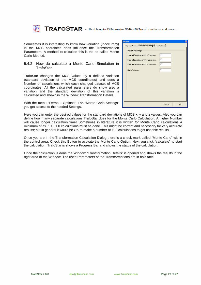
Sometimes it is interesting to know how variation (inaccuracy) in the MCS coordintes does influence the Transformation Parameters. A method to calculate this is the so called Monte Carlo Method. 5.4.2 How do calculate a Monte Carlo Simulation in

TrafoStar TrafoStar changes the MCS values by a defined variation (standard deviation of the MCS coordinates) and does a Number of calculations which each changed dataset of MCS coordinates. All the calculated parameters do show also a variation and the standard deviation of this variation is calculated and shown in the Window Transformation Details. With the menu “Extras – Options”; Tab “Monte Carlo Settings” you get access to the needed Settings. Here you can enter the desired values for the standard deviations of MCS x, y and z values. Also you can define how many separate calculations TrafoStar does for the Monte Carlo Calculation. A higher Number will cause longer calculation time! Sometimes in literature it is written for Monte Carlo calculations a minimum of ex. 100.000 calculations must be done. This might be correct and necessary for very accurate results; but in general it would be OK to make a number of 100 calculations to get useable results. Once you are in the Transformation Calculation Dialog there is a check mark called “Monte Carlo” within the control area. Check this Button to activate the Monte Carlo Option. Next you click “calculate” to start the calculation. TrafoStar is shows a Progress Bar and shows the status of the calculation. Once the calculation is done the Window “Transformation Details” is opened and shows the results in the right area of the Window. The used Parameters of the Transformations are in bold face.

TrafoStar 2.0.0

[email protected]


5.4.3 Reasonable usage of Monte Carlo Method Specially within Paraboloid Transformations (see chapter 5.2) the standard deviations of the Parameters do not show the real situation, because they are only calculated from the fitting of the points to the shape. 5.5 Inverse Transformation Parameters [Form Transformation Calculation, Button Details, information in Top right Frame] The inverse Transformation Parameters are defined as the parameters which transform a point from the target system (OCS) back to the start system (MCS) based on the general Transformation equation. In Matrix Notation this is: (NOTE: OCS is the Target System and MCS the Start System)

OCS = TRA + Rot_Matrix * Affine_Matrix * Scale_Matr ix * MCS

or

Σ⋅⋅⋅+=Σ sART´ Formula 1

Where is: Σ = Coordinates in Start system MCS [x, y, z] T

Σ´= Coordinates in Target system OCS [x´, y´, z´] T

T = Translation Matrix [tx, ty, tz]T

R = Rotation Matrix from Rx, Ry´ and Rz´´ (see 13.1 - Rotation Matrix)

TrafoStar 2.0.0

[email protected]


A = Affine Matrix (see 13.3 - Affine Matrix ) s = Scale Matrix (see 13.2 - Scale Matrix Formula 1 can be converted to:

( )TRAs −Σ⋅⋅⋅=Σ −−− ´111 Formula 2

and next step into:

´111111 Σ⋅⋅⋅+⋅⋅⋅−=Σ −−−−−− RAsTRAs Formula 3

The inverse Translation T´ can easily be calculated by TRAsT ⋅⋅⋅−= −−− 111´ . (T´ is the translation to transform a Point form Target System (OCS = Σ´) to Start System (MCS = Σ); by definition the Translation Vector is parallel to the final System which is MCS in this case, so the inverse Translation Vector T´ is parallel to the MCS = Start System.) The inverse Parameters for Scale (s´), Rotation (R´) and Affine Parameters (A´) must be found from the

equation ´´´111 sARRAs ⋅⋅=⋅⋅ −−− . TrafoStar is doing this calculations. The inverse Transformation Parameters are identically with the Parameters you get if you SWAP the Transformation direction manually (make Target Points to Start Points and make Start Points to Target Points). You have this effect directly in TrafoStar by clicking the button "MCS <=> OCS"). 5.5.1 Specialities on Transformations and inverse Parameters by doing calculations with

separate scale parameters on any single Axis There is a special thing on transformations with scale parameters used on single axis like scale x, scale y and / or scale z. For example on a 9 Parameter Transformation (3 translations, 3 rotations and 3 scales) with following Points MCS

1 1.000000 2.000000 3.000000 2 4.000000 8.000000 99.000000 3 33.000000 45.000000 -33.000000 4 23.000000 44.000000 -6.000000 5 -66.000000 77.000000 8.000000

OCS

1 -8.467688 22.839304 48.430798 2 -26.126433 76.146287 160.163982 3 59.102764 26.354724 9.524298 4 42.978551 44.846388 36.956362 5 -12.247603 131.599740 6.827676

=> You get zero rest-deviation in all Points.

TrafoStar 2.0.0

[email protected]


If you manually transverse the calculation by taking the OCS Points as MCS Points and the MCS Points as OCS Points and do again a 9 Parameter Transformation you get the following deviations:

1 2.268 -0.896 -1.499 2 -3.011 0.997 1.959 3 -0.975 0.510 -1.901 4 -1.437 0.630 -0.828 5 3.156 -1.241 2.270

So in one Transformation Direction you have a perfect fit and in the other direction your get big deviations. How is that possible? Based on the TrafoStars fundamental Transformation formula

OCS = TRA + Rot_Matrix * Affine_Matrix * Scale_Matr ix * MCS

TrafoStar is transforming points from the Start System to the Target System. An Example with Scales: First transform MCS to OCS (with Rotation in z and two different and large scales in x and y)

=> with Rotation and different Scale in x and y

Transformation for the inverse Parameters (OCS back to MCS; but OCS Points are now defined as Start Points and MCS as Target Points):

=> with Rotation and different Scale in x and y (FIRST Scale, then rotate!)

x

y

x´

y´

x x´

y´ y

TrafoStar 2.0.0

[email protected]


It is not possible to get the rectangle back to a square with scales which are not parallel to the sides of the rectangle (Note: The Order of Rotation and Scale is importand, based on the fundamental Transformatin Equation scale is done FIRST, then SECOND rotation) This can also be shown based on matrix calculations (Translations and Affine Parameters are not relevant for this problem):

Σ⋅⋅=Σ sR´ and ´11 Σ⋅⋅=Σ −− Rs

and for Σ we are looking for a formula in Type of ´´´ Σ⋅⋅sR

So the job is to find the matrices R´and s´ for R´• s´ equals the result of s-1 • R-1. As R´ is a rotation Matrix it has to be a orthogonal Matrix and s´ must have the structure of a scale Matrix (which is a Diagonal Matrix see 13.2 - Scale Matrix). The result of s-1 • R-1 is a Matrix, and this Matrix has to be converted into a orthogonal Matrix (= R´) and a Scale Matrix ( = s´) what is not possible. Well known is a conversion of a matrix A to Q • R, where Q is a orthogonal Matrix and R is a upper triangular Matrix (Iwasawa Partition). This shows the inverse Transformation Parameters do not exist if there are multiple scales, but because the Affine Matrix is a upper triangle Matrix there is a solution for the inverse Parameters if affine parameters are used. Also for the given Example above the deviations go to zero on every Point if a 12 Parameter Transformation is calculated with Start = OCS and MCS = Target. 5.6 Multiple Solutions The rotation between two coordinate Systems has two possible ways, for example for a x, y´and z´´ order one solution could be 0°,0°,0° and the other 180°,180°,180°. If you make a transformation with rotations AND affine Parameters you could have EIGHT equal solutions. The reason is the affine solution its own has two solutions (for example: xy, ztoxy and azimuth: 5°, 5°, 5° and the other 5°, -5°, 185° => if you calculate the affine matrix with both sets you get the same matrix. The combination of rotation and affine parameters gives one more general solution for rotation with the second rotation solution and also one more general solution for the affine solution. For example the Rotation 1°, 2°, 3° and the affine Parameters 4°, 5° and 6° do have the following equal solutions:

Solution 1 Solution 2 Solution 3 Solution 4 Solution 5 Solution 6 Solution 7 Solution 8 tra x 0 0 0 0 0 0 0 0 tra y 0 0 0 0 0 0 0 0 tra z 0 0 0 0 0 0 0 0 rot x -179 -179 1 1 1 1 -179 -179 rot y' 178 178 2 2 178 178 2 2 rot z'' -177 -177 3 3 -177 -177 3 3

scale x 1.000000 1.000000 1.000000 1.000000 1.000000 1.000000 1.000000 1.000000 scale y 1.000000 1.000000 1.000000 1.000000 1.000000 1.000000 1.000000 1.000000 scale z 1.000000 1.000000 1.000000 1.000000 1.000000 1.000000 1.000000 1.000000

xy 4 4 4 4 176 176 176 176 Azimuth z -175 5 -175 5 -5 175 -5 175

z to xy -6 6 -6 6 174 -174 174 -174

TrafoStar 2.0.0

[email protected]


Within the Form Transformation Calculation you can toggle between this solutions by clicking three buttons: "sec Rot Sol" toggles between the two Rotation solutions "sec Aff Sol" toggles between the two Affine solutions "Show alternative Rot / Affine Solution" gives the general second solution, now the two other buttons toggle between the "local" rotation and Affine solutions. 6 Usage of Windows Clipboard (see also Chapter 8.1 - Print „Screen-DEFAULT“ to Clipboard - CTRL + D) (see also Chapter 11 – Menu Extras – Options) In the Menu Extras – Options the clipboard settings can be made. For bigger number of points it is recommended to use the setting “Do not copy anything to clipboard” because it needs some time to copy everything to the clipboard.

The setting “Complete results to clipboard after each calculation” copies the results to the Windows Clipboard automatically. From here you can copy the Data to other applications. In the picture below the content of the clipboard is shown. The first 12 rows contain the transformation parameters. If a parameter is not used in the transformation here the neutral value of the parameter is shown (e.g. 1 for a scale). After this the statistical values are shown. The following rows contain the identical Points (Point ID, MCS x, MCS y, MCS z, OCS x, OCS y, OCS z, dev.x, dev.y, dev.z).

TrafoStar 2.0.0

[email protected]


„BMW Cell Calibration Component Parameters" are special conventions of transformation parameters. The Values tra x, tra y, tra z, -rot x, -rot y, -rot z are copied to the Windows clipboard. For the result it is important in which direction the data is transformed. If Robot Data (ABC Angles or Quaternion's) is used, this data can only be imported as OCS = Target Data, but often the Robot Data is the Start System and any other Data the Target System. So if the convention is to transform vice versa, you can get this results into the clipboard by checking the checkbox "give inverted Parameters to Clipboard" and the inverse Transformation Parameters are copied. (Regarding inverse Parameters see 5.5 - Inverse Transformation Parameters) 7 The Main Sheet The Main Sheet shows all Data in the OCS Coordinate System! If no transformation has yet been calculated the values for all MCS Points are 0! In the first rows the identically points are shown (Green Point ID Field). Next the Points which are only in the MCS File are shown (yellow Point ID Field). Then the Points which are only in the OCS File are shown (orange Point ID Filed). After done transformation all Points are shown in the OCS coordinate system. The points which are only in the MCS (=Start) File so will be subsequent transformed with the parameters calculated based on the identically points. Parts of the table can be highlighted and copied to the windows clipboard or can be shown in a 2D Diagram by right mouse click on the area. 7.1 Rectangular, cylindrical and spherical coordina te systems Coordinates are always imported as rectangular coordinates (x, y, z). The calculation to cylindrical or spherical coordinates is always done in TrafoStar. It is every time based on the z Axis of the rectangular system as the reference axis between both system definitions. So for axample on the cylindrical system z equals H. 8 The Graphics Window - Screen The Graphics Window is opened and closed by the Menu Graphics – Graphics Window. You can open more than one Graphics Window, but only one of this is the default window, this is written in the top frame of the Graphics Window.

TrafoStar 2.0.0

[email protected]


8.1 Print „Screen-DEFAULT“ to Clipboard - CTRL + D The content of the Graphics Window is copied to the clipboard with the menu Graphics - Print „Screen-DEFAULT“ to Clipboard or with the shortcut „Ctrl + D“. 8.2 More Settings with the menu Graphics The data representation can be manipulated with: Right mouse button zooms out Left mouse button and drag sector zoom Ctrl + left mouse button translate Shift + left mouse button rotate Shift + left mouse button + right mouse button rotate around the axis perpendicular to your screen Mouse Wheel zooms in and out Ctrl + c centre the graphics Ctrl + a zoom to all Ctrl + s side view Ctrl + t top view Ctrl + f front view Ctrl + u set point of rotation Key left translate left Key right translate right Key up translate up Key down translate down Shift + Key left positive rotation around left – right axis of screen Shift + Key right negative rotation around left – right axis of screen Shift + Key up positive rotation around bottom – top axis of screen Shift + Key down negative rotation around bottom – top axis of screen Shift + L positive rotation around axis perpendicular to screen Shift + R negative rotation around axis perpendicular to screen

TrafoStar 2.0.0

[email protected]


F5 Flags Mode: Mode to set flags by clicking a point on the screen F6 dynamic Flag: Show Flag for closed point to mouse cursor, hit F6 again and Flag

stays F7 Black Plane Dialog F8 Line Mode, draw lines between points Ctrl + v show deviation vectors Ctrl + y Analyse-Mode (Points move along their deviation vectors) Ctrl + L make vectors longer (alternative F3 in Analyze Mode) Ctrl + h make vectors shorter (alternative F4 in Analyze Mode) Ctrl + k keep points – In Analyze Mode the moved Point stays on the screen Ctrl + b show points bigger (big) Ctrl + m show pints smaller (small) Ctrl + p Show Points just as one Pixel Ctrl + r Show tolerance bar

Ctrl + e Show details of Tolerance Bar settings (can also be done by a double click onto

the color bar in the ColorBar window) 8.3 ColorBar

With the ColorBar the visualization of the Colors and Deviations are controlled. The Deviation Vectors can be shown as components of rectangular, cylindrical or spherical coordinate systems. This is chosen in the “Coordinate System Type”. With a change of this option the Text of the Checkboxes in “Show rules” and in “plus minus rules” changes also. All Settings which are made in the ColorBar are stored within a saved View.

TrafoStar 2.0.0

[email protected]


The following pictures show the settings in the ColorBar with a chosen cylindrical Coordinate system type.

With the „Show rules“ any component could be switched on and off. It is a special issue the 3D deviation vectors do not have an algebraic sign and is always positive (because it IS a 3D deviation!). So once you show all 3D Deviations on the screen they would only use the positive side of the color bar. It would give a more transparent and clear view by using also the negative colors for the vectors. So it is possible to define the color of a deviation vector by the “plus minus rules”. For example if you only look at the transverse deviations (Phi component) it could make sense to switch the “plus minus rules” to “based on ve.Phi”. The Option “based on ABS dev” uses only the positive side of the color bar. You can show one, two or three components of the deviation vector and you can choose based on which component the color bar is used. So the color is linked to the algebraic sign of only ONE component. However, you decide on your own, what makes sense and what not! The Option “Show only in Trafo used Component of Vector“ does only show the deviation vectors which components have been used in the transformation. „Show ve.xyz Component“ turns ON all three components of each vector. The Check Button „Set min and max on every Vector Settings change“ sets the plus and minus tolerance to the maximum positive value if any change is made in the ColorBar settings. If for example only the Phi components are shown the max and min value will become to the max Value of the Phi component automatically. With the „Grid Options“ a coordinate Grid can be shown and manipulated.

TrafoStar 2.0.0

[email protected]


8.4 Lines

With the Menu „Graphics – Lines – Line Mode Active“ or with the Icon or by <F8> the line mode is turned on. In this mode lines as connection between points can be added to the graphics (only MCS Points can be used). Do draw a line set Line mode active, chose “Set line” and click next to a point. On every click close to a point a new line will be drawn and a polygon is added to screen. A double click stops the actual drawing; you can start a new polygon by clicking to another point. With “Delete Line” drawn lines can be deleted. If you turn off the Line Mode no lines will be shown any more. Once you turn line mode on, the lines will be shown again.

8.5 Black Plane The function „Black Plane“ allows to control the visibility of points by two parallel and virtual planes; called the black

TrafoStar 2.0.0

[email protected]


Planes. All Points between these planes stay visible, all other points become invisible. You can open the Dialog by F7 or with the Menu “Graphics - Black Plane”. Once you click “Activate Black Plane” two planes parallel to the actual graphics view are initialized. These planes are shown when you click “Show Black Planes Borders in Screen”. Hit Apply or OK to make changes active. The Planes are shown in the centre of the graphics window. If you translate or rotate the graphics view the planes move with the view, so these planes are defined in the same coordinate system as the points. With pressing „t“ and mouse movement the distance between the two planes (t = thickness) changes.

With pressing „b“ and mouse movement both planes are moved parallel to them selves (b = Basis). All Points outside the two planes are invisible and all Points between the two planes are shown. So with logical initialisation of the planes (graphics view / rotation must make sense) the visibility of points can be controlled.

After finishing the movements of the planes the graphics can be used as known. Within the black plane dialog the two planes can be set invisible (checkbox “Show Black Planes Borders in Screen”), but it stays active! Also the planes can be initialized again by clicking “Initialize Planes”.

TrafoStar 2.0.0

[email protected]


8.6 Menü Global Graphics The Menu “Global Graphics - General Graphics Settings” gives access to the Dialog „Graphics Options“. Here general settings fort he graphics window can be made. These Settings are NOT stored with a saved view. But these settings are stored into the TrafoStar.ini File, so they stay unchanged by the next start of TrafoStar. The visibility of point Groups (OCS, MCS, only OCS, only MCS; “only” means the Point is not an identically point and is only existing in MCS or OCS) is controlled by the Settings in “Visible Points in Graphics”. The chapter “…more Settings…” has some different possibilities:

� “Show closer Points bigger” draws the points, which are “closer” to the user bigger, this gives a better 3D View; closer means the direction perpendicular to the screen

� “Show ColorBar in Graphics Window” switches the color bar in the Graphics on and off

� “Show Vectors as thick as Points” shows the deviation Vectors in the same thickness than the points

� “Show Quaternion Vector” switches the Quaternion Vector in the Graphics on and off

� “Show R Dist Vectors and REAL dx, ….” shows in case of a transformation with a R_Dist Parameter (constant distance between identical points) the total Vector (including the Distance) between the identical Points. So you can analyze in which direction the vector is pointing

TrafoStar 2.0.0

[email protected]


9 Save graphical Views

You can save views of the Graphics screen with the Icon Bar or the Menu Views. Once the views are saved you can recall them with the drop down box or with the Menu. After the click on the Icon „Save View“ a Dialog appears. Here you can enter a name for the view to save.

A saved View is recalled (and will be shown in the DEFAULT Graphics Window) by selecting an item from the drop down box. “Ctrl + z” and “Ctrl + y” is kind of a undo function for the graphics screen (also use the corresponding Icons) 10 Flags By clicking the Icon

or entering the Menu „Graphics – Flags Mode“ the Flags Mode is active and Flags can be set by clicking next to a point (also use F5). An active Flags Mode is visualized by a different mouse cursor over the graphics screen:

By clicking a point in the graphics window a flag is set close to the point. The flag contains a table with the point’s data. By double click on this flag you can edit the flags table and do some settings on the flags.

TrafoStar 2.0.0

[email protected]


If you save a view all flags are stored with the view. The option „Snap to invisible Grid“ puts the flags exactly on a invisible Grid, which is visible once you drag the flag. The Grid length can be defined by the user. If you choose “change all Flags to new settings“ all already set flags are set to the actual in the Edit Flag window made settings. The option „put Flag on all visible Points“ sets to all visible points in screen a flag with the actual settings. 11 Menu Extras – Options In this Menu the storage of results in the windows clipboard is controlled. (The storage is done every time the button “Calculate” in the transformation calculation dialog is hit). See Chapter 6 - Usage of Windows Clipboard.

TrafoStar 2.0.0

[email protected]


“Do not copy anything to clipboard” – no Data is copied to the Clipboard “Complete results to clipboard after each calculation” “Robot measurement protocol results after each calculation” – not yet released „BMW Cell Calibration Component Parameters“ - The parameters Translation x, y and z and the rotation x, y and z (rotations with inverse algebraic sign) are copied to the clipboard 12 More functions 12.1 Export of RobCad *.rf Files (See also 5.3 - Ro bot Base measurements) The Menu „File - Export - RobCad *.rf“ File exports the transformation results (the Parameter Translation x, y und z and Rotation around x, y and z) into a *.rf File. This function is often used to tell RobCad the relationship between a fixture and a robot. Therefore you must have a Number of n identically Points in booth coordinate systems (The Robot and the fixture system, often the fixture represents the object coordinate system, like a car, plane, etc.). To get these points, the robot drives into n positions and its end effectors 3D Position is measured by a 3D measurement System in the fixtures coordinate system. ATTENTION: In MCS (Start System) the coordinates of the Robot (Base System) are defined In OCS (Target System) the coordinates of the fixture / Object / Car are defined With the Export a *.rf File is created. The parameters Place, Fixture and Robot must be entered and these will be stored in the File also. In the rf File the 3 Translations and the Rotations (z, y’ and x’’) in the order x’’, y’ and z are stored (also the algebraic sign of the rotations is flipped).

TrafoStar 2.0.0

[email protected]


100

0cossin

0sincos

αααα −

=zR

αααβ

cossin0

sincos0

001

−=xR

13 Basics of overdetermined 3D Transformations The 3D Transformation between MCS (= Start) and OCS (= Target) is calculated with the equation:

OCS = TRA + Rot_Matrix * Affine_Matrix * Scale_Matr ix * MCS Here in is: OCS Object Coordinate System = Target System TRA Vector of Translation Rot_Matrix Rotation-matrix (calculated from the three rotations around x, y’ and z’’; so this are the

rotations around the already rotated axes, this is defined by the ‘ and ‘’) Affine_Matrix Matrix of affine Parameter Scale_Matrix Matrix of the scales MCS Measurement Coordinate System = Start System The equation shows in detail the way the parameters are defined and how the coordinates from the MCS = Start System are transformed to the Target = OCS System Important is the place of the Translation. In this equation the Translation is done AFTER the Rotation, that means the resulting translation values are defined in the TARGET = OCS Coordinate system. The algebraic sign of the rotation is based on the rules of positive rotation in mathematics (for example a Rotation around z is positive if the x Axis is turned to the y Axis on the shortest way). 13.1 Rotation Matrix

+α x

y

x’

y’

+β y

z

y’

z’

TrafoStar 2.0.0

[email protected]


γγ

γγ

cos0sin

010

sin0cos

−=yR

−+−−−+

=⋅⋅=βαβαβ

γβαγαγβαγαγβγβαγαγβαγαγβ

coscoscossinsin

sinsincoscossinsinsinsincoscossincos

cossincossinsincossinsinsincoscoscos

xyzxyz RRRR

13.2 Scale Matrix The Scale Matrix has the following structure:

=sz

sy

sx

Scale

00

00

00

13.3 Affine Matrix The affine parameters are used to define a non rectangular coordinate system. xy Deviation from 90 degrees between the positive x and y Axis Azimuth z Azimuth of the z Axis (projected into the xy plane); reference for the angle azimuth = 0 is

the positive x axis z to xy Deviation from 90 degrees between the z Axis and the xy plane The Affine Matrix has the following structure (with xy = Angle between x and y Axis, ztoxy = Angle from z Axis to xy plane and Az = Azimuth of z Axis projected to xy plane).

⋅⋅

=cos(ztoxy)00

sin(Az) sin(ztoxy)cos(xy)0

cos(Az) sin(ztoxy)sin(xy)1

Affin

13.4 R Dist Value The „R_Dist“ parameter is available since Version 1.3.69. It defines a constant distance in 3D Space (only the distance itself is constant, not the vector of this distance) between the identical points. To calculate the 3D BestFit with this parameter every Distance in Space gets a correction (and this one is minimized during

+γ z

x

z’

x’

TrafoStar 2.0.0

[email protected]


the least square adjustment). Finally this correction is separated into its x, y and z component and shown in TrafoStar. The equation fort he R_Dist Value is the following: R_Dist + v = SQR (OCSx - MCSx) ^ 2+(OCSy - MCSy) ^ 2+(OCSz - MCSz) ^ 2) With OCS = TRA + Rot_Matrix * Affine_Matrix * Scale_Matrix * MCS ATTENTION: The subsequent Transformation of Points is done WITHOUT the R_Dist Value, it doesn’t matter if it was calculated during the BestFit Transformation. The reason is the forward Transformation is not defined with the R_Dist value (Because of the unknown vector of the R_Dist). Practical Examples fort the usages of R_Dist Transformations are: - Measurement of Robot Bases if the TCP of the Robot is not known and the measured Point is eccentric mounted to the TCP (see 5.3 - Robot Base measurements) - Connection of Coordinate Systems without having the line of sight between identically Points; if it is possible to set artefacts (like Scale bars) between the points, the length of the artefacts is the R_Dist Value. If this value is known it can be calculated with the “R Data is known” option, net yet released) - Analysis of measured data with regards to Offsets or additional constants (R0 Values) 14 Versions Version 2.0.36; Jan 30th, 2014

- Etta Value in ini File gives access to quicker iterations; can help on files with large numbers; be carefully with changing this value!

- Clipboard Export Option (Menue Extras – Options) copies X, Y, Z, A, B, C to clipboard (X = Trala x, Y = Trala y, Z = Trala z, A = -rot z, B = - rot y, C = - rot x)

Version 2.0.37; Feb 09th, 2014

- Change of Units has direct effect to Window “Transformation Calculation” - Added info about used Units in Window “Transformation Calculation” - Complete new code for Paraboloid Fit, better and more stable iteration, more stable results - Added Units to clipboard option “Complete results to clipboard after each calculation” - Changed behaviour of “use Parameter” Checkboxes in Window “Transformation Calculation”; the

last calculated parameter value will remain in the Textbox once Checkbox is unchecked; click checkbox again and Parameter is “float”, click it again and Parameter is “0”

Version 2.0.38; Feb 23rd, 2014

- New MonteCarlo Functionality, enter Standard Deviations of your MCS Coordinates and get the Standard Deviations of your calculated Transformation Parameters done by a Monte Carlo calculation

Version 2.0.39; March 01st 2014

- Window Transformation Calculation can be copied into Windows Clipboard by clicking new button “copy to clipboard”

- Value “sigma xyz” is also in clipboard after calculation when Menu “Extras – Options”; Tab “Clipboard Settings” “Complete Results to clipboard after each calculation” is set.

- New Option for visibility of Points; Menu “Global Graphics” – “General Graphics Settings” – Checkbox “don’t View Points which are out of Tol.”; if this Box is checked no out of Tolerance

TrafoStar 2.0.0

[email protected]


Point is shown in the graphics Window (Tolerance can be set here: “Graphics” – “Tolerance” – “Color Bar”

Version 2.0.40; May 13th 2014

- fixed bug when using FileBrowse Button in BatchTransform - fixed bug when using Explore Button in BatchTransform in Windows 7 Operating System

Version 2.0.41, May 27th 2014

- fixed bug in Graphics Window when showing the OCS Points and MCS Points (Menu General Graphics Settings)

Version 2.0.42, Sept. 20th 2014

- added the option for the R_Dist calculation to use Robots ABC Angle which could be imported by *.dat File (Kuka Format); see chapter 5.3.3.

Version 2.0.47, April, 7th 2015 (2.0.43 to 2.0.46 are internal releases)

- added calculation of inverse Transformation Parameters - added some more detailed information to pdf Manual regarding scale and affine parameters - added new Rotation sequence in Form Details - usage of Quaternion's possible for R-Dist calculation, added a new simple Format for import - done some finale things and issues on saving ABC Angels and Quaternion's to *.tfo Files - added new functionality on Auto Find Points for Importing Points without identical Names (rename

OCS or MCS Point Names based on the corresponding Name) Version 2.0.48, April 24th 2015

- fixed bug with ini Files when installing TrafoStar on new computer Version 2.0.49, April 3rd 2016

- new Unit FEET available in Dialog UNITS - COMMA "," is allowed as separator in Input files (only if Computer Settings for Decimal delimiter

are POINT ".". Version 2.0.50, May 26th 2016

- fixed major bug in Transformation which was causing crash on some computers Version 2.0.51, August 29th 2016

- fixed a bug which occurred while i importing data on systems with comma as decimal delimiter Version 2.0.52, January 24th 2017

- added the Rotation sequence z y' z'' to the Details Dialog within the Transformations Calculation Dialog

Version 2.0.53, April 02nd 2017

- fixed little Bug while using Special Macro for Transforming couple of PointSets given in Microsoft Excel

TrafoStar 2.0.0

[email protected]


15 Contact Contact TrafoStar: [email protected] www.TrafoStar.com

Date post:	12-Mar-2018
Category:	Documents
Upload:	dangthien
View:	220 times
Download:	0 times

Handbuch TrafoStar English 2.0 TrafoStar English 2... · 12.1 Export of RobCad *.rf Files ......

Documents