MIT 6.02 DRAFT Lecture NotesFall 2011 (Last update: October 9, 2011)Comments, questions or bug reports?

Please contact hari at mit.edu

CHAPTER 8Viterbi Decoding of Convolutional

Codes

This chapter describes an elegant and efficient method to decode convolutional codes,whose construction and encoding we described in the previous chapter. This decodingmethod avoids explicitly enumerating the 2N possible combinations of N-bit parity bitsequences. This method was invented by Andrew Viterbi ’57 and bears his name.

� 8.1 The Problem

At the receiver, we have a sequence of voltage samples corresponding to the parity bits thatthe transmitter has sent. For simplicity, and without loss of generality, we will assume thatthe receiver picks a suitable sample for the bit, or better still, averages the set of samplescorresponding to a bit, digitizes that value to a “0” or “1” by comparing to the thresholdvoltage (the demapping step), and propagates that bit decision to the decoder.

Thus, we have a received bit sequence, which for a convolutionally coded stream cor-responds to the stream of parity bits. If we decode this received bit sequence with noother information from the receiver’s sampling and demapper, then the decoding processis termed hard decision decoding (“hard decoding”). If, in addition, the decoder is giventhe actual voltage samples and uses that information in decoding the data, we term theprocess soft decision decoding (“soft decoding”).

The Viterbi decoder can be used in either case. Intuitively, because hard decision de-coding makes an early decision regarding whether a bit is 0 or 1, it throws away infor-mation in the digitizing process. It might make a wrong decision, especially for voltagesnear the threshold, introducing a greater number of bit errors in the received bit sequence.Although it still produces the most likely transmitted sequence given the received bit se-quence, by introducing additional errors in the early digitization, the overall reduction inthe probability of bit error will be smaller than with soft decision decoding. But it is con-ceptually easier to understand hard decoding, so we will start with that, before going onto soft decoding.

As mentioned in the previous chapter, the trellis provides a good framework for un-

1

2 CHAPTER 8. VITERBI DECODING OF CONVOLUTIONAL CODES

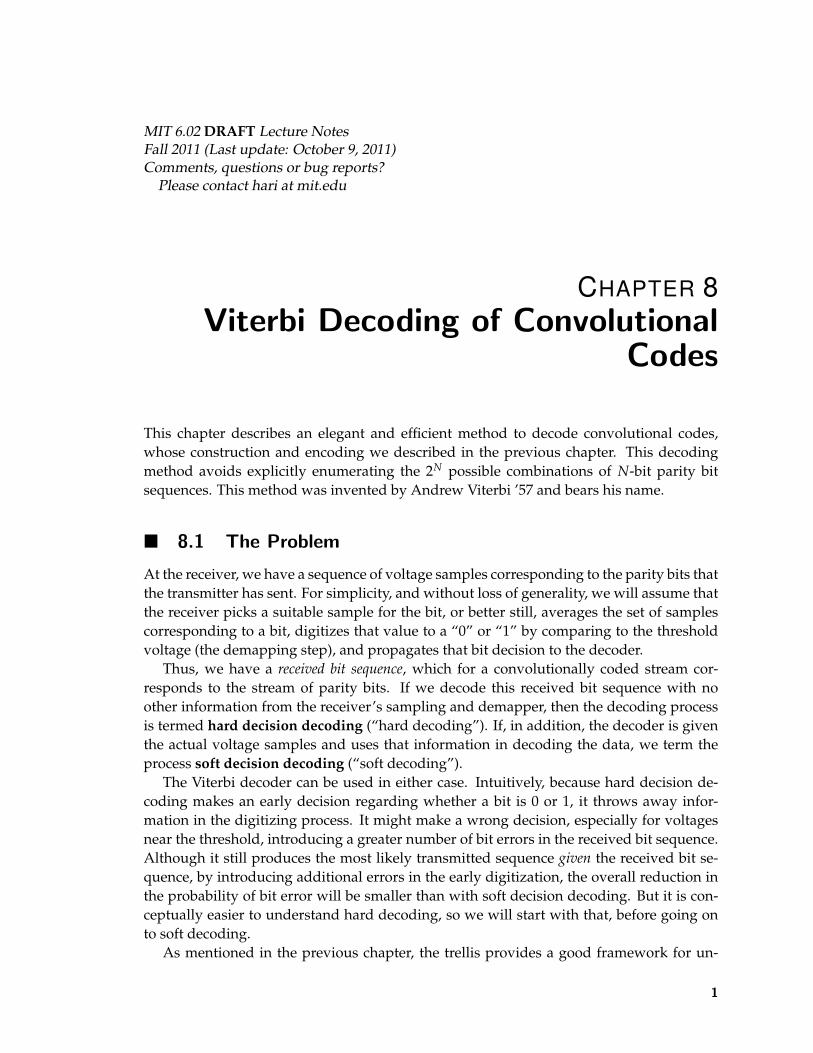
Figure 8-1: The trellis is a convenient way of viewing the decoding task and understanding the time evo-lution of the state machine.

derstanding the decoding procedure for convolutional codes (Figure 8-1). Suppose wehave the entire trellis in front of us for a code, and now receive a sequence of digitizedbits (or voltage samples). If there are no errors (i.e., the signal-to-noise ratio, SNR, is highenough), then there will be some path through the states of the trellis that would exactlymatch the received sequence. That path (specifically, the concatenation of the encoding ofeach state along the path) corresponds to the transmitted parity bits. From there, gettingto the original message is easy because the top arc emanating from each node in the trelliscorresponds to a “0” bit and the bottom arrow corresponds to a “1” bit.

When there are bit errors, what can we do? As explained earlier, finding the most likelytransmitted message sequence is appealing because it minimizes the BER. If we can comeup with a way to capture the errors introduced by going from one state to the next, thenwe can accumulate those errors along a path and come up with an estimate of the totalnumber of errors along the path. Then, the path with the smallest such accumulation oferrors is the path we want, and the transmitted message sequence can be easily determinedby the concatenation of states explained above.

To solve this problem, we need a way to capture any errors that occur in going throughthe states of the trellis, and a way to navigate the trellis without actually materializing theentire trellis (i.e., without enumerating all possible paths through it and then finding theone with smallest accumulated error). The Viterbi decoder solves these problems. It isan example of a more general approach to solving optimization problems, called dynamicprogramming. Later in the course, we will apply similar concepts in network routing, anunrelated problem, to find good paths in multi-hop networks.

SECTION 8.2. THE VITERBI DECODER 3

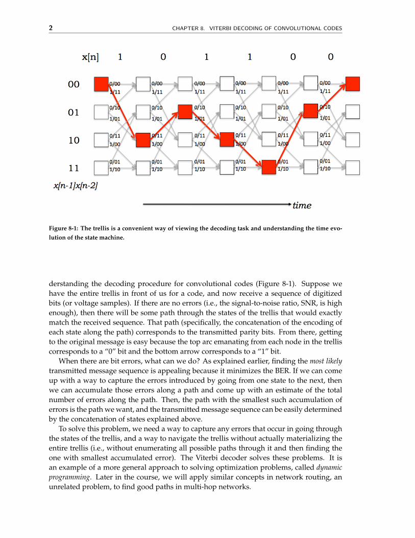
Figure 8-2: The branch metric for hard decision decoding. In this example, the receiver gets the parity bits00.

� 8.2 The Viterbi Decoder

The decoding algorithm uses two metrics: the branch metric (BM) and the path metric(PM). The branch metric is a measure of the “distance” between what was transmitted andwhat was received, and is defined for each arc in the trellis. In hard decision decoding,where we are given a sequence of digitized parity bits, the branch metric is the Hammingdistance between the expected parity bits and the received ones. An example is shown inFigure 8-2, where the received bits are 00. For each state transition, the number on the arcshows the branch metric for that transition. Two of the branch metrics are 0, correspondingto the only states and transitions where the corresponding Hamming distance is 0. Theother non-zero branch metrics correspond to cases when there are bit errors.

The path metric is a value associated with a state in the trellis (i.e., a value associatedwith each node). For hard decision decoding, it corresponds to the Hamming distanceover the most likely path from the initial state to the current state in the trellis. By “mostlikely”, we mean the path with smallest Hamming distance between the initial state andthe current state, measured over all possible paths between the two states. The path withthe smallest Hamming distance minimizes the total number of bit errors, and is most likelywhen the BER is low.

The key insight in the Viterbi algorithm is that the receiver can compute the path metricfor a (state, time) pair incrementally using the path metrics of previously computed statesand the branch metrics.

� 8.2.1 Computing the Path Metric

Suppose the receiver has computed the path metric PM[s, i] for each state s at time stepi (recall that there are 2K−1 states, where K is the constraint length of the convolutionalcode). In hard decision decoding, the value of PM[s, i] is the total number of bit errorsdetected when comparing the received parity bits to the most likely transmitted message,considering all messages that could have been sent by the transmitter until time step i(starting from state “00”, which we will take to be the starting state always, by convention).

4 CHAPTER 8. VITERBI DECODING OF CONVOLUTIONAL CODES

Among all the possible states at time step i, the most likely state is the one with thesmallest path metric. If there is more than one such state, they are all equally good possi-bilities.

Now, how do we determine the path metric at time step i + 1, PM[s, i + 1], for each states? To answer this question, first observe that if the transmitter is at state s at time step i + 1,then it must have been in only one of two possible states at time step i. These two predecessorstates, labeled α and β, are always the same for a given state. In fact, they depend onlyon the constraint length of the code and not on the parity functions. Figure 8-2 shows thepredecessor states for each state (the other end of each arrow). For instance, for state 00,α = 00 and β = 01; for state 01, α = 10 and β = 11.

Any message sequence that leaves the transmitter in state s at time i + 1 must have leftthe transmitter in state α or state β at time i. For example, in Figure 8-2, to arrive in state’01’ at time i + 1, one of the following two properties must hold:

1. The transmitter was in state ‘10’ at time i and the ith message bit was a 0. If that isthe case, then the transmitter sent ‘11’ as the parity bits and there were two bit errors,because we received the bits 00. Then, the path metric of the new state, PM[‘01’, i + 1]is equal to PM[‘10’, i] + 2, because the new state is ‘01’ and the corresponding pathmetric is larger by 2 because there are 2 errors.

2. The other (mutually exclusive) possibility is that the transmitter was in state ‘11’ attime i and the ith message bit was a 0. If that is the case, then the transmitter sent 01as the parity bits and tere was one bit error, because we received 00. The path metricof the new state, PM[‘01’, i + 1] is equal to PM[‘11’, i] + 1.

Formalizing the above intuition, we can see that

PM[s, i + 1] = min(PM[α, i] + BM[α → s],PM[β, i] + BM[β → s]), (8.1)

where α and β are the two predecessor states.In the decoding algorithm, it is important to remember which arc corresponds to the

minimum, because we need to traverse this path from the final state to the initial onekeeping track of the arcs we used, and then finally reverse the order of the bits to producethe most likely message.

� 8.2.2 Finding the Most Likely Path

We can now describe how the decoder finds the maximum-likelihood path. Initially, state‘00’ has a cost of 0 and the other 2k−1 − 1 states have a cost of ∞.

The main loop of the algorithm consists of two main steps: first, calculating the branchmetric for the next set of parity bits, and second, computing the path metric for the nextcolumn. The path metric computation may be thought of as an add-compare-select proce-dure:

1. Add the branch metric to the path metric for the old state.2. Compare the sums for paths arriving at the new state (there are only two such paths

to compare at each new state because there are only two incoming arcs from theprevious column).

3. Select the path with the smallest value, breaking ties arbitrarily. This path corre-sponds to the one with fewest errors.

SECTION 8.3. SOFT DECISION DECODING 5

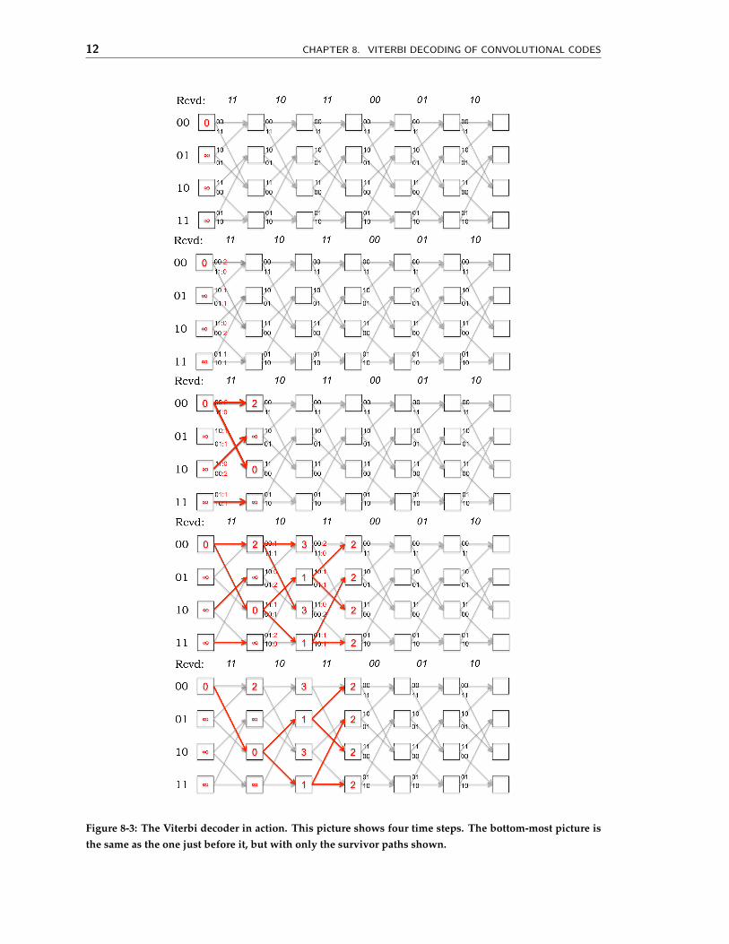
Figure 8-3 shows the decoding algorithm in action from one time step to the next. Thisexample shows a received bit sequence of 11 10 11 00 01 10 and how the receiver processesit. The fourth picture from the top shows all four states with the same path metric. At thisstage, any of these four states and the paths leading up to them are most likely transmittedbit sequences (they all have a Hamming distance of 2). The bottom-most picture showsthe same situation with only the survivor paths shown. A survivor path is one that hasa chance of being the maximum-likelihood path; there are many other paths that can bepruned away because there is no way in which they can be most likely. The reason whythe Viterbi decoder is practical is that the number of survivor paths is much, much smallerthan the total number of paths in the trellis.

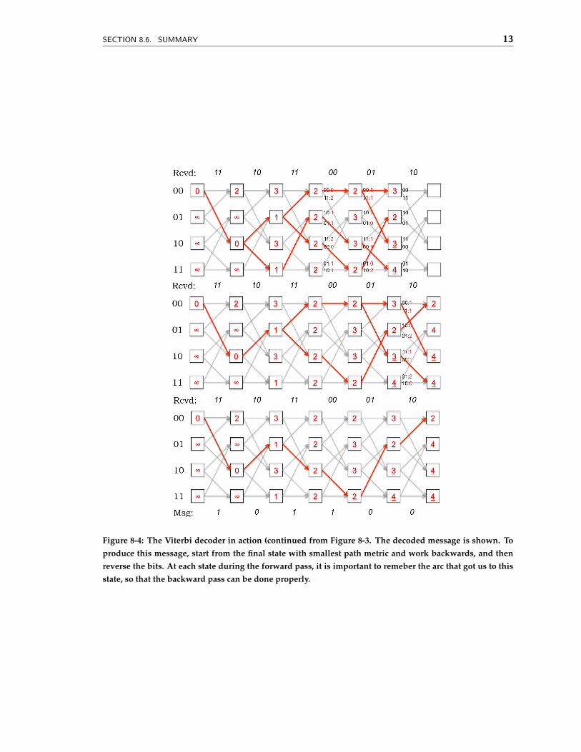
Another important point about the Viterbi decoder is that future knowledge will help itbreak any ties, and in fact may even cause paths that were considered “most likely” at acertain time step to change. Figure 8-4 continues the example in Figure 8-3, proceeding un-til all the received parity bits are decoded to produce the most likely transmitted message,which has two bit errors.

� 8.3 Soft Decision Decoding

Hard decision decoding digitizes the received voltage signals by comparing it to a thresh-old, before passing it to the decoder. As a result, we lose information: if the voltage was0.500001, the confidence in the digitization is surely much lower than if the voltage was0.999999. Both are treated as “1”, and the decoder now treats them the same way, eventhough it is overwhelmingly more likely that 0.999999 is a “1” compared to the other value.

Soft decision decoding (also sometimes known as “soft input Viterbi decoding”) buildson this observation. It does not digitize the incoming samples prior to decoding. Rather, it usesa continuous function of the analog sample as the input to the decoder. For example, if theexpected parity bit is 0 and the received voltage is 0.3 V, we might use 0.3 (or 0.32, or somesuch function) as the value of the “bit” instead of digitizing it.

For technical reasons that will become apparent later, an attractive soft decision metricis the square of the difference between the received voltage and the expected one. If theconvolutional code produces p parity bits, and the p corresponding analog samples arev = v1, v2, . . . , vp, one can construct a soft decision branch metric as follows

BMsoft[u, v] =p

∑i=1

(ui − vi)2, (8.2)

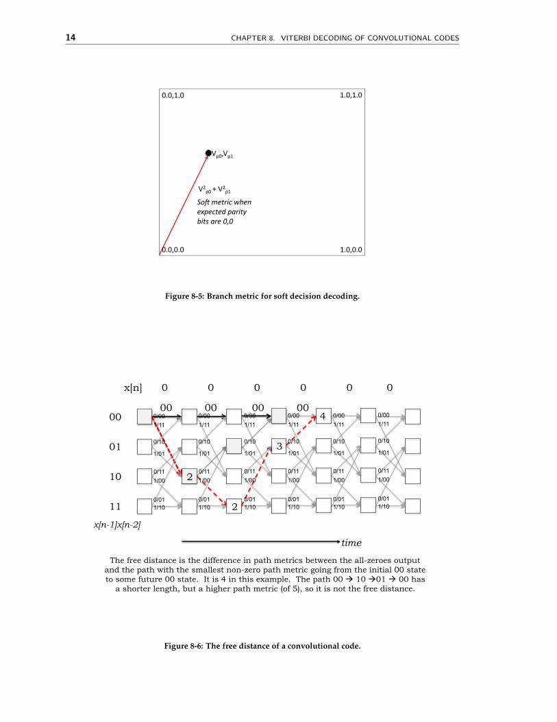
where u = u1, u2, . . . , up are the expected p parity bits (each a 0 or 1). Figure 8-5 shows thesoft decision branch metric for p = 2 when u is 00.

With soft decision decoding, the decoding algorithm is identical to the one previouslydescribed for hard decision decoding, except that the branch metric is no longer an integerHamming distance but a positive real number (if the voltages are all between 0 and 1, thenthe branch metric is between 0 and 1 as well).

It turns out that this soft decision metric is closely related to the probability of the decodingbeing correct when the channel experiences additive Gaussian noise. First, let’s look at thesimple case of 1 parity bit (the more general case is a straightforward extension). Suppose

6 CHAPTER 8. VITERBI DECODING OF CONVOLUTIONAL CODES

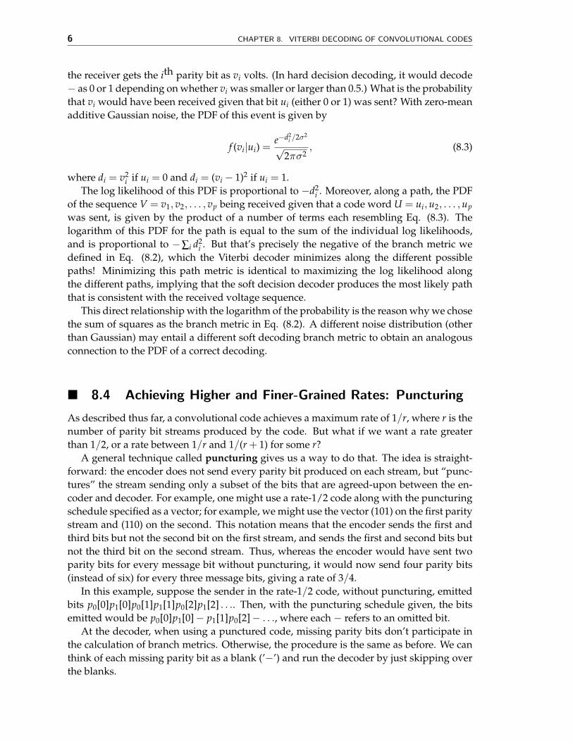
the receiver gets the ith parity bit as vi volts. (In hard decision decoding, it would decode− as 0 or 1 depending on whether vi was smaller or larger than 0.5.) What is the probabilitythat vi would have been received given that bit ui (either 0 or 1) was sent? With zero-meanadditive Gaussian noise, the PDF of this event is given by

f (vi|ui) =e−d2

i /2σ2

√2πσ2

, (8.3)

where di = v2i if ui = 0 and di = (vi − 1)2 if ui = 1.

The log likelihood of this PDF is proportional to −d2i . Moreover, along a path, the PDF

of the sequence V = v1, v2, . . . , vp being received given that a code word U = ui, u2, . . . , up

was sent, is given by the product of a number of terms each resembling Eq. (8.3). Thelogarithm of this PDF for the path is equal to the sum of the individual log likelihoods,and is proportional to −∑i d2

i . But that’s precisely the negative of the branch metric wedefined in Eq. (8.2), which the Viterbi decoder minimizes along the different possiblepaths! Minimizing this path metric is identical to maximizing the log likelihood alongthe different paths, implying that the soft decision decoder produces the most likely paththat is consistent with the received voltage sequence.

This direct relationship with the logarithm of the probability is the reason why we chosethe sum of squares as the branch metric in Eq. (8.2). A different noise distribution (otherthan Gaussian) may entail a different soft decoding branch metric to obtain an analogousconnection to the PDF of a correct decoding.

� 8.4 Achieving Higher and Finer-Grained Rates: Puncturing

As described thus far, a convolutional code achieves a maximum rate of 1/r, where r is thenumber of parity bit streams produced by the code. But what if we want a rate greaterthan 1/2, or a rate between 1/r and 1/(r + 1) for some r?

A general technique called puncturing gives us a way to do that. The idea is straight-forward: the encoder does not send every parity bit produced on each stream, but “punc-tures” the stream sending only a subset of the bits that are agreed-upon between the en-coder and decoder. For example, one might use a rate-1/2 code along with the puncturingschedule specified as a vector; for example, we might use the vector (101) on the first paritystream and (110) on the second. This notation means that the encoder sends the first andthird bits but not the second bit on the first stream, and sends the first and second bits butnot the third bit on the second stream. Thus, whereas the encoder would have sent twoparity bits for every message bit without puncturing, it would now send four parity bits(instead of six) for every three message bits, giving a rate of 3/4.

In this example, suppose the sender in the rate-1/2 code, without puncturing, emittedbits p0[0]p1[0]p0[1]p1[1]p0[2]p1[2] . . .. Then, with the puncturing schedule given, the bitsemitted would be p0[0]p1[0]− p1[1]p0[2]− . . ., where each − refers to an omitted bit.

At the decoder, when using a punctured code, missing parity bits don’t participate inthe calculation of branch metrics. Otherwise, the procedure is the same as before. We canthink of each missing parity bit as a blank (’−’) and run the decoder by just skipping overthe blanks.

SECTION 8.5. PERFORMANCE ISSUES 7

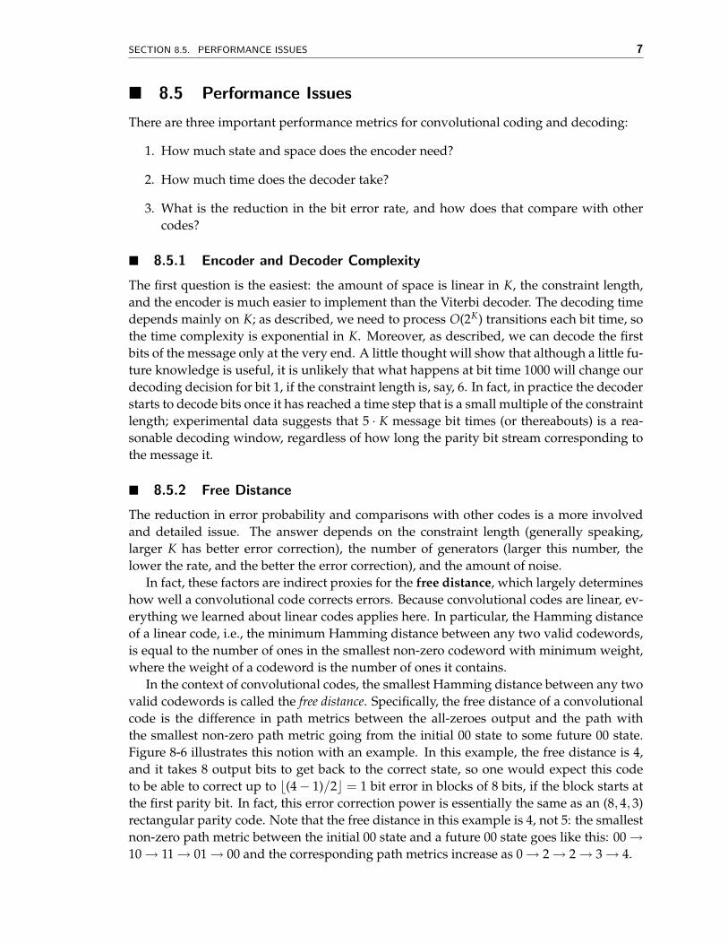
� 8.5 Performance Issues

There are three important performance metrics for convolutional coding and decoding:

1. How much state and space does the encoder need?

2. How much time does the decoder take?

3. What is the reduction in the bit error rate, and how does that compare with othercodes?

� 8.5.1 Encoder and Decoder Complexity

The first question is the easiest: the amount of space is linear in K, the constraint length,and the encoder is much easier to implement than the Viterbi decoder. The decoding timedepends mainly on K; as described, we need to process O(2K) transitions each bit time, sothe time complexity is exponential in K. Moreover, as described, we can decode the firstbits of the message only at the very end. A little thought will show that although a little fu-ture knowledge is useful, it is unlikely that what happens at bit time 1000 will change ourdecoding decision for bit 1, if the constraint length is, say, 6. In fact, in practice the decoderstarts to decode bits once it has reached a time step that is a small multiple of the constraintlength; experimental data suggests that 5 · K message bit times (or thereabouts) is a rea-sonable decoding window, regardless of how long the parity bit stream corresponding tothe message it.

� 8.5.2 Free Distance

The reduction in error probability and comparisons with other codes is a more involvedand detailed issue. The answer depends on the constraint length (generally speaking,larger K has better error correction), the number of generators (larger this number, thelower the rate, and the better the error correction), and the amount of noise.

In fact, these factors are indirect proxies for the free distance, which largely determineshow well a convolutional code corrects errors. Because convolutional codes are linear, ev-erything we learned about linear codes applies here. In particular, the Hamming distanceof a linear code, i.e., the minimum Hamming distance between any two valid codewords,is equal to the number of ones in the smallest non-zero codeword with minimum weight,where the weight of a codeword is the number of ones it contains.

In the context of convolutional codes, the smallest Hamming distance between any twovalid codewords is called the free distance. Specifically, the free distance of a convolutionalcode is the difference in path metrics between the all-zeroes output and the path withthe smallest non-zero path metric going from the initial 00 state to some future 00 state.Figure 8-6 illustrates this notion with an example. In this example, the free distance is 4,and it takes 8 output bits to get back to the correct state, so one would expect this codeto be able to correct up to b(4− 1)/2c = 1 bit error in blocks of 8 bits, if the block starts atthe first parity bit. In fact, this error correction power is essentially the same as an (8,4,3)rectangular parity code. Note that the free distance in this example is 4, not 5: the smallestnon-zero path metric between the initial 00 state and a future 00 state goes like this: 00 →10 → 11 → 01 → 00 and the corresponding path metrics increase as 0 → 2 → 2 → 3 → 4.

8 CHAPTER 8. VITERBI DECODING OF CONVOLUTIONAL CODES

Why do we define a “free distance”, rather than just call it the Hamming distance, if itis defined the same way? The reason is that any code with Hamming distance D (whetherlinear or not) can correct all patterns of up to bD−1

2 c errors. If we just applied the samenotion to convolutional codes, we will conclude that we can correct all single-bit errors inthe example given, or in general, we can correct some fixed number of errors.

Now, convolutional coding produces an unbounded bit stream; these codes aremarkedly distinct from block codes in this regard. As a result, the bD−1

2 c formula is nottoo instructive because it doesn’t capture the true error correction properties of the code.A convolutional code (with Viterbi decoding) can correct t = bD−1

2 c errors as long as theseerrors are “far enough apart”. So the notion we use is the free distance because, in a sense,errors can keep occurring and as long as no more than t of them occur in a closely spacedburst, the decoder can correct them all.

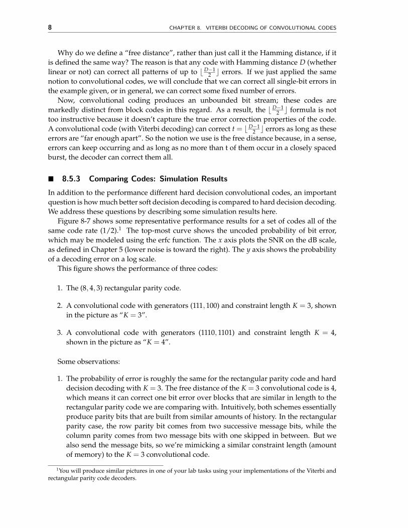
� 8.5.3 Comparing Codes: Simulation Results

In addition to the performance different hard decision convolutional codes, an importantquestion is how much better soft decision decoding is compared to hard decision decoding.We address these questions by describing some simulation results here.

Figure 8-7 shows some representative performance results for a set of codes all of thesame code rate (1/2).1 The top-most curve shows the uncoded probability of bit error,which may be modeled using the erfc function. The x axis plots the SNR on the dB scale,as defined in Chapter 5 (lower noise is toward the right). The y axis shows the probabilityof a decoding error on a log scale.

This figure shows the performance of three codes:

1. The (8,4,3) rectangular parity code.

2. A convolutional code with generators (111,100) and constraint length K = 3, shownin the picture as “K = 3”.

3. A convolutional code with generators (1110,1101) and constraint length K = 4,shown in the picture as “K = 4”.

Some observations:

1. The probability of error is roughly the same for the rectangular parity code and harddecision decoding with K = 3. The free distance of the K = 3 convolutional code is 4,which means it can correct one bit error over blocks that are similar in length to therectangular parity code we are comparing with. Intuitively, both schemes essentiallyproduce parity bits that are built from similar amounts of history. In the rectangularparity case, the row parity bit comes from two successive message bits, while thecolumn parity comes from two message bits with one skipped in between. But wealso send the message bits, so we’re mimicking a similar constraint length (amountof memory) to the K = 3 convolutional code.

1You will produce similar pictures in one of your lab tasks using your implementations of the Viterbi andrectangular parity code decoders.

SECTION 8.6. SUMMARY 9

2. The probability of error for a given amount of noise is noticeably lower for the K = 4code compared to K = 3 code; the reason is that the free distance of this K = 4 code is6, and it takes 7 trellis edges to achieve that (000→ 100→ 010→ 001→ 000), meaningthat the code can correct up to 2 bit errors in sliding windows of length 2 · 4 = 8 bits.

3. The probability of error for a given amount of noise is dramatically lower with softdecision decoding than hard decision decoding. In fact, K = 3 and soft decodingbeats K = 4 and hard decoding in these graphs. For a given error probability (andsignal), the degree of noise that can be tolerated with soft decoding is much higher(about 2.5–3 dB, which is a good rule-of-thumb to apply in practice for the gain fromsoft decoding, all other things being equal).

Figure 8-8 shows a comparison of three different convolutional codes together with theuncoded case. Two of the codes are the same as in Figure 8-7, i.e., (111,110) and (1110,1101);these were picked because they were recommended by Bussgang’s paper. The third codeis (111,101), with parity equations

p0[n] = x[n] + x[n− 1] + x[n− 2]

p1[n] = x[n] + x[n− 2].

The results of this comparison are shown in Figure 8-8. These graphs show the prob-ability of decoding error (BER after decoding) for experiments that transmit messages oflength 500,000 bits each. (Because the BER of the best codes in this set are on the order of10−6, we actually need to run the experiment over even longer messages when the SNR ishigher than 3 dB; that’s why we don’t see results for one of the codes, where the experi-ment encountered no errors.)

Interestingly, these results show that the code (111,101) is stronger than the other twocodes, even though its constraint length, 3, is smaller than that of (1110,1101). To under-stand why, we can calculate the free distance of this code, which turns out to be 5. This freedistance is smaller than that of (1110,1101), whose free distance is 6, but the number of trel-lis edges to go from state 00 back to state 00 in the (111,101) case is only 3, corresponding toa 6-bit block. The relevant state transitions are 00 → 10 → 01 → 00 and the correspondingpath metrics are 0 → 2 → 3 → 5. Hence, its error correcting power is marginally strongerthan the (1110,1101) code.

� 8.6 Summary

From its relatively modest, though hugely impactful, beginnings as a method to decodeconvolutional codes, Viterbi decoding has become one of the most widely used algorithmsin a wide range of fields and engineering systems. Modern disk drives with “PRML”technology to speed-up accesses, speech recognition systems, natural language systems,and a variety of communication networks use this scheme or its variants.

In fact, a more modern view of the soft decision decoding technique described in thislecture is to think of the procedure as finding the most likely set of traversed states ina Hidden Markov Model (HMM). Some underlying phenomenon is modeled as a Markovstate machine with probabilistic transitions between its states; we see noisy observations

10 CHAPTER 8. VITERBI DECODING OF CONVOLUTIONAL CODES

from each state, and would like to piece together the observations to determine the mostlikely sequence of states traversed. It turns out that the Viterbi decoder is an excellentstarting point to solve this class of problems (and sometimes the complete solution).

On the other hand, despite its undeniable success, Viterbi decoding isn’t the only wayto decode convolutional codes. For one thing, its computational complexity is exponentialin the constraint length, K, because it does require each of these states to be enumerated.When K is large, one may use other decoding methods such as BCJR or Fano’s sequentialdecoding scheme, for instance.

Convolutional codes themselves are very popular over both wired and wireless links.They are sometimes used as the “inner code” with an outer block error correcting code,but they may also be used with just an outer error detection code. They are also usedas a component in more powerful codes line turbo codes, which are currently one of thehighest-performing codes used in practice.

� Problems and Exercises

1. Please check out and solve the online problems on error correction codes athttp://web.mit.edu/6.02/www/f2011/handouts/tutprobs/ecc.html

2. Consider a convolutional code whose parity equations are

p0[n] = x[n] + x[n− 1] + x[n− 3]

p1[n] = x[n] + x[n− 1] + x[n− 2]

p2[n] = x[n] + x[n− 2] + x[n− 3]

(a) What is the rate of this code? How many states are in the state machine repre-sentation of this code?

(b) Suppose the decoder reaches the state “110” during the forward pass of theViterbi algorithm with this convolutional code.

i. How many predecessor states (i.e., immediately preceding states) does state“110” have?

ii. What are the bit-sequence representations of the predecessor states of state“110”?

iii. What are the expected parity bits for the transitions from each of these pre-decessor states to state “110”? Specify each predecessor state and the ex-pected parity bits associated with the corresponding transition below.

(c) To increase the rate of the given code, Lem E. Tweakit punctures the p0 paritystream using the vector (1 0 1 1 0), which means that every second and fifth bitproduced on the stream are not sent. In addition, she punctures the p1 paritystream using the vector (1 1 0 1 1). She sends the p2 parity stream unchanged.What is the rate of the punctured code?

3. Let conv encode(x) be the resulting bit-stream after encoding bit-string x with aconvolutional code, C. Similarly, let conv decode(y) be the result of decoding yto produce the maximum-likelihood estimate of the encoded message. Suppose we

SECTION 8.6. SUMMARY 11

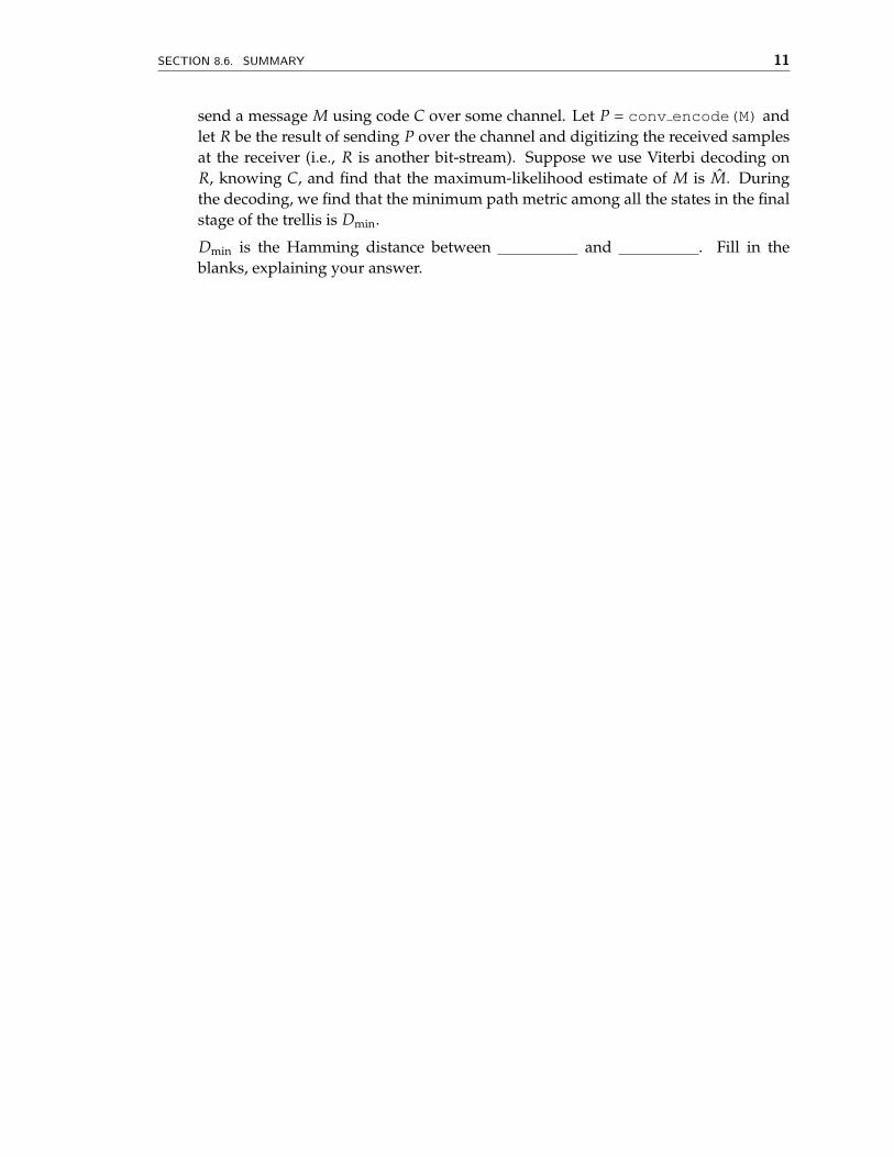
send a message M using code C over some channel. Let P = conv encode(M) andlet R be the result of sending P over the channel and digitizing the received samplesat the receiver (i.e., R is another bit-stream). Suppose we use Viterbi decoding onR, knowing C, and find that the maximum-likelihood estimate of M is M̂. Duringthe decoding, we find that the minimum path metric among all the states in the finalstage of the trellis is Dmin.

Dmin is the Hamming distance between and . Fill in theblanks, explaining your answer.

12 CHAPTER 8. VITERBI DECODING OF CONVOLUTIONAL CODES

Figure 8-3: The Viterbi decoder in action. This picture shows four time steps. The bottom-most picture isthe same as the one just before it, but with only the survivor paths shown.

SECTION 8.6. SUMMARY 13

Figure 8-4: The Viterbi decoder in action (continued from Figure 8-3. The decoded message is shown. Toproduce this message, start from the final state with smallest path metric and work backwards, and thenreverse the bits. At each state during the forward pass, it is important to remeber the arc that got us to thisstate, so that the backward pass can be done properly.

14 CHAPTER 8. VITERBI DECODING OF CONVOLUTIONAL CODES

0.0,1.0   1.0,1.0  

Vp0,Vp1  

So#  metric  when  expected  parity  bits  are  0,0  

0.0,0.0   1.0,0.0  

V2p0  +  V2

p1  

Figure 8-5: Branch metric for soft decision decoding.

00

01

10

11

0/00 1/11

0/10

1/01

1/00 0/11

0/01 1/10

time

x[n-1]x[n-2]

x[n] 0 0 0 0 0 0

0/00 1/11

0/10

1/01

1/00 0/11

0/01 1/10

0/00 1/11

0/10

1/01

1/00 0/11

0/01 1/10

0/00 1/11

0/10

1/01

1/00 0/11

0/01 1/10

0/00 1/11

0/10

1/01

1/00 0/11

0/01 1/10

0/00 1/11

0/10

1/01

1/00 0/11

0/01 1/10

2

00 00 00

The free distance is the difference in path metrics between the all-zeroes output and the path with the smallest non-zero path metric going from the initial 00 state to some future 00 state. It is 4 in this example. The path 00 à 10 à01 à 00 has

a shorter length, but a higher path metric (of 5), so it is not the free distance.

2

3

4 00

Figure 8-6: The free distance of a convolutional code.

SECTION 8.6. SUMMARY 15

Figure 8-7: Error correcting performance results for different rate-1/2 codes.

Figure 8-8: Error correcting performance results for three different rate-1/2 convolutional codes. The pa-rameters of the three convolutional codes are (111,110) (labeled “K = 3 glist=(7,6)”), (1110,1101) (labeled“K = 4 glist=(14,13)”), and (111,101) (labeled “K = 3 glist=(7,5)”). The top three curves below the uncodedcurve are for hard decision decoding; the bottom three curves are for soft decision decoding.