133
Advanced Design System 2011.01 - Harmonic Balance Simulation 1 Advanced Design System 2011.01 Feburary 2011 Harmonic Balance Simulation

Advanced Design System 2011.01 - Harmonic Balance Simulation
1
Advanced Design System 2011.01
Feburary 2011Harmonic Balance Simulation
Advanced Design System 2011.01 - Harmonic Balance Simulation
2
© Agilent Technologies, Inc. 2000-20115301 Stevens Creek Blvd., Santa Clara, CA 95052 USANo part of this documentation may be reproduced in any form or by any means (includingelectronic storage and retrieval or translation into a foreign language) without prioragreement and written consent from Agilent Technologies, Inc. as governed by UnitedStates and international copyright laws.
AcknowledgmentsMentor Graphics is a trademark of Mentor Graphics Corporation in the U.S. and othercountries. Mentor products and processes are registered trademarks of Mentor GraphicsCorporation. * Calibre is a trademark of Mentor Graphics Corporation in the US and othercountries. "Microsoft®, Windows®, MS Windows®, Windows NT®, Windows 2000® andWindows Internet Explorer® are U.S. registered trademarks of Microsoft Corporation.Pentium® is a U.S. registered trademark of Intel Corporation. PostScript® and Acrobat®are trademarks of Adobe Systems Incorporated. UNIX® is a registered trademark of theOpen Group. Oracle and Java and registered trademarks of Oracle and/or its affiliates.Other names may be trademarks of their respective owners. SystemC® is a registeredtrademark of Open SystemC Initiative, Inc. in the United States and other countries and isused with permission. MATLAB® is a U.S. registered trademark of The Math Works, Inc..HiSIM2 source code, and all copyrights, trade secrets or other intellectual property rightsin and to the source code in its entirety, is owned by Hiroshima University and STARC.FLEXlm is a trademark of Globetrotter Software, Incorporated. Layout Boolean Engine byKlaas Holwerda, v1.7 http://www.xs4all.nl/~kholwerd/bool.html . FreeType Project,Copyright (c) 1996-1999 by David Turner, Robert Wilhelm, and Werner Lemberg.QuestAgent search engine (c) 2000-2002, JObjects. Motif is a trademark of the OpenSoftware Foundation. Netscape is a trademark of Netscape Communications Corporation.Netscape Portable Runtime (NSPR), Copyright (c) 1998-2003 The Mozilla Organization. Acopy of the Mozilla Public License is at http://www.mozilla.org/MPL/ . FFTW, The FastestFourier Transform in the West, Copyright (c) 1997-1999 Massachusetts Institute ofTechnology. All rights reserved.
The following third-party libraries are used by the NlogN Momentum solver:
"This program includes Metis 4.0, Copyright © 1998, Regents of the University ofMinnesota", http://www.cs.umn.edu/~metis , METIS was written by George Karypis([email protected]).
Intel@ Math Kernel Library, http://www.intel.com/software/products/mkl
SuperLU_MT version 2.0 - Copyright © 2003, The Regents of the University of California,through Lawrence Berkeley National Laboratory (subject to receipt of any requiredapprovals from U.S. Dept. of Energy). All rights reserved. SuperLU Disclaimer: THISSOFTWARE IS PROVIDED BY THE COPYRIGHT HOLDERS AND CONTRIBUTORS "AS IS"AND ANY EXPRESS OR IMPLIED WARRANTIES, INCLUDING, BUT NOT LIMITED TO, THEIMPLIED WARRANTIES OF MERCHANTABILITY AND FITNESS FOR A PARTICULAR PURPOSEARE DISCLAIMED. IN NO EVENT SHALL THE COPYRIGHT OWNER OR CONTRIBUTORS BELIABLE FOR ANY DIRECT, INDIRECT, INCIDENTAL, SPECIAL, EXEMPLARY, ORCONSEQUENTIAL DAMAGES (INCLUDING, BUT NOT LIMITED TO, PROCUREMENT OFSUBSTITUTE GOODS OR SERVICES; LOSS OF USE, DATA, OR PROFITS; OR BUSINESS
Advanced Design System 2011.01 - Harmonic Balance Simulation
3
INTERRUPTION) HOWEVER CAUSED AND ON ANY THEORY OF LIABILITY, WHETHER INCONTRACT, STRICT LIABILITY, OR TORT (INCLUDING NEGLIGENCE OR OTHERWISE)ARISING IN ANY WAY OUT OF THE USE OF THIS SOFTWARE, EVEN IF ADVISED OF THEPOSSIBILITY OF SUCH DAMAGE.
7-zip - 7-Zip Copyright: Copyright (C) 1999-2009 Igor Pavlov. Licenses for files are:7z.dll: GNU LGPL + unRAR restriction, All other files: GNU LGPL. 7-zip License: This libraryis free software; you can redistribute it and/or modify it under the terms of the GNULesser General Public License as published by the Free Software Foundation; eitherversion 2.1 of the License, or (at your option) any later version. This library is distributedin the hope that it will be useful,but WITHOUT ANY WARRANTY; without even the impliedwarranty of MERCHANTABILITY or FITNESS FOR A PARTICULAR PURPOSE. See the GNULesser General Public License for more details. You should have received a copy of theGNU Lesser General Public License along with this library; if not, write to the FreeSoftware Foundation, Inc., 59 Temple Place, Suite 330, Boston, MA 02111-1307 USA.unRAR copyright: The decompression engine for RAR archives was developed using sourcecode of unRAR program.All copyrights to original unRAR code are owned by AlexanderRoshal. unRAR License: The unRAR sources cannot be used to re-create the RARcompression algorithm, which is proprietary. Distribution of modified unRAR sources inseparate form or as a part of other software is permitted, provided that it is clearly statedin the documentation and source comments that the code may not be used to develop aRAR (WinRAR) compatible archiver. 7-zip Availability: http://www.7-zip.org/
AMD Version 2.2 - AMD Notice: The AMD code was modified. Used by permission. AMDcopyright: AMD Version 2.2, Copyright © 2007 by Timothy A. Davis, Patrick R. Amestoy,and Iain S. Duff. All Rights Reserved. AMD License: Your use or distribution of AMD or anymodified version of AMD implies that you agree to this License. This library is freesoftware; you can redistribute it and/or modify it under the terms of the GNU LesserGeneral Public License as published by the Free Software Foundation; either version 2.1 ofthe License, or (at your option) any later version. This library is distributed in the hopethat it will be useful, but WITHOUT ANY WARRANTY; without even the implied warranty ofMERCHANTABILITY or FITNESS FOR A PARTICULAR PURPOSE. See the GNU LesserGeneral Public License for more details. You should have received a copy of the GNULesser General Public License along with this library; if not, write to the Free SoftwareFoundation, Inc., 51 Franklin St, Fifth Floor, Boston, MA 02110-1301 USA Permission ishereby granted to use or copy this program under the terms of the GNU LGPL, providedthat the Copyright, this License, and the Availability of the original version is retained onall copies.User documentation of any code that uses this code or any modified version ofthis code must cite the Copyright, this License, the Availability note, and "Used bypermission." Permission to modify the code and to distribute modified code is granted,provided the Copyright, this License, and the Availability note are retained, and a noticethat the code was modified is included. AMD Availability:http://www.cise.ufl.edu/research/sparse/amd
UMFPACK 5.0.2 - UMFPACK Notice: The UMFPACK code was modified. Used by permission.UMFPACK Copyright: UMFPACK Copyright © 1995-2006 by Timothy A. Davis. All RightsReserved. UMFPACK License: Your use or distribution of UMFPACK or any modified versionof UMFPACK implies that you agree to this License. This library is free software; you canredistribute it and/or modify it under the terms of the GNU Lesser General Public Licenseas published by the Free Software Foundation; either version 2.1 of the License, or (at
Advanced Design System 2011.01 - Harmonic Balance Simulation
4
your option) any later version. This library is distributed in the hope that it will be useful,but WITHOUT ANY WARRANTY; without even the implied warranty of MERCHANTABILITYor FITNESS FOR A PARTICULAR PURPOSE. See the GNU Lesser General Public License formore details. You should have received a copy of the GNU Lesser General Public Licensealong with this library; if not, write to the Free Software Foundation, Inc., 51 Franklin St,Fifth Floor, Boston, MA 02110-1301 USA Permission is hereby granted to use or copy thisprogram under the terms of the GNU LGPL, provided that the Copyright, this License, andthe Availability of the original version is retained on all copies. User documentation of anycode that uses this code or any modified version of this code must cite the Copyright, thisLicense, the Availability note, and "Used by permission." Permission to modify the codeand to distribute modified code is granted, provided the Copyright, this License, and theAvailability note are retained, and a notice that the code was modified is included.UMFPACK Availability: http://www.cise.ufl.edu/research/sparse/umfpack UMFPACK(including versions 2.2.1 and earlier, in FORTRAN) is available athttp://www.cise.ufl.edu/research/sparse . MA38 is available in the Harwell SubroutineLibrary. This version of UMFPACK includes a modified form of COLAMD Version 2.0,originally released on Jan. 31, 2000, also available athttp://www.cise.ufl.edu/research/sparse . COLAMD V2.0 is also incorporated as a built-infunction in MATLAB version 6.1, by The MathWorks, Inc. http://www.mathworks.com .COLAMD V1.0 appears as a column-preordering in SuperLU (SuperLU is available athttp://www.netlib.org ). UMFPACK v4.0 is a built-in routine in MATLAB 6.5. UMFPACK v4.3is a built-in routine in MATLAB 7.1.
Qt Version 4.6.3 - Qt Notice: The Qt code was modified. Used by permission. Qt copyright:Qt Version 4.6.3, Copyright (c) 2010 by Nokia Corporation. All Rights Reserved. QtLicense: Your use or distribution of Qt or any modified version of Qt implies that you agreeto this License. This library is free software; you can redistribute it and/or modify it undertheterms of the GNU Lesser General Public License as published by the Free SoftwareFoundation; either version 2.1 of the License, or (at your option) any later version. Thislibrary is distributed in the hope that it will be useful,but WITHOUT ANY WARRANTY; without even the implied warranty of MERCHANTABILITYor FITNESS FOR A PARTICULAR PURPOSE. See the GNU Lesser General Public License formore details. You should have received a copy of the GNU Lesser General Public Licensealong with this library; if not, write to the Free Software Foundation, Inc., 51 Franklin St,Fifth Floor, Boston, MA 02110-1301 USA Permission is hereby granted to use or copy thisprogram under the terms of the GNU LGPL, provided that the Copyright, this License, andthe Availability of the original version is retained on all copies.Userdocumentation of any code that uses this code or any modified version of this code mustcite the Copyright, this License, the Availability note, and "Used by permission."Permission to modify the code and to distribute modified code is granted, provided theCopyright, this License, and the Availability note are retained, and a notice that the codewas modified is included. Qt Availability: http://www.qtsoftware.com/downloads PatchesApplied to Qt can be found in the installation at:$HPEESOF_DIR/prod/licenses/thirdparty/qt/patches. You may also contact BrianBuchanan at Agilent Inc. at [email protected] for more information.
The HiSIM_HV source code, and all copyrights, trade secrets or other intellectual propertyrights in and to the source code, is owned by Hiroshima University and/or STARC.
Advanced Design System 2011.01 - Harmonic Balance Simulation
5
Errata The ADS product may contain references to "HP" or "HPEESOF" such as in filenames and directory names. The business entity formerly known as "HP EEsof" is now partof Agilent Technologies and is known as "Agilent EEsof". To avoid broken functionality andto maintain backward compatibility for our customers, we did not change all the namesand labels that contain "HP" or "HPEESOF" references.
Warranty The material contained in this document is provided "as is", and is subject tobeing changed, without notice, in future editions. Further, to the maximum extentpermitted by applicable law, Agilent disclaims all warranties, either express or implied,with regard to this documentation and any information contained herein, including but notlimited to the implied warranties of merchantability and fitness for a particular purpose.Agilent shall not be liable for errors or for incidental or consequential damages inconnection with the furnishing, use, or performance of this document or of anyinformation contained herein. Should Agilent and the user have a separate writtenagreement with warranty terms covering the material in this document that conflict withthese terms, the warranty terms in the separate agreement shall control.
Technology Licenses The hardware and/or software described in this document arefurnished under a license and may be used or copied only in accordance with the terms ofsuch license. Portions of this product include the SystemC software licensed under OpenSource terms, which are available for download at http://systemc.org/ . This software isredistributed by Agilent. The Contributors of the SystemC software provide this software"as is" and offer no warranty of any kind, express or implied, including without limitationwarranties or conditions or title and non-infringement, and implied warranties orconditions merchantability and fitness for a particular purpose. Contributors shall not beliable for any damages of any kind including without limitation direct, indirect, special,incidental and consequential damages, such as lost profits. Any provisions that differ fromthis disclaimer are offered by Agilent only.
Restricted Rights Legend U.S. Government Restricted Rights. Software and technicaldata rights granted to the federal government include only those rights customarilyprovided to end user customers. Agilent provides this customary commercial license inSoftware and technical data pursuant to FAR 12.211 (Technical Data) and 12.212(Computer Software) and, for the Department of Defense, DFARS 252.227-7015(Technical Data - Commercial Items) and DFARS 227.7202-3 (Rights in CommercialComputer Software or Computer Software Documentation).
Advanced Design System 2011.01 - Harmonic Balance Simulation
6
Harmonic Balance Basics . . . . . . . . . . . . . . . . . . . . . . . . . . . . . . . . . . . . . . . . . . . . . . . . . . . 7 Overview . . . . . . . . . . . . . . . . . . . . . . . . . . . . . . . . . . . . . . . . . . . . . . . . . . . . . . . . . . . . 7 Using Harmonic Balance Simulation . . . . . . . . . . . . . . . . . . . . . . . . . . . . . . . . . . . . . . . . . . 8 Examples of Harmonic Balance Simulation . . . . . . . . . . . . . . . . . . . . . . . . . . . . . . . . . . . . . 9 Reference Equations . . . . . . . . . . . . . . . . . . . . . . . . . . . . . . . . . . . . . . . . . . . . . . . . . . . . 14 Limitations . . . . . . . . . . . . . . . . . . . . . . . . . . . . . . . . . . . . . . . . . . . . . . . . . . . . . . . . . . . 14 HB Simulation Parameters . . . . . . . . . . . . . . . . . . . . . . . . . . . . . . . . . . . . . . . . . . . . . . . . 14 Theory of Operation . . . . . . . . . . . . . . . . . . . . . . . . . . . . . . . . . . . . . . . . . . . . . . . . . . . . . 34 Troubleshooting a Simulation . . . . . . . . . . . . . . . . . . . . . . . . . . . . . . . . . . . . . . . . . . . . . . 42
Harmonic Balance for Nonlinear Noise Simulation . . . . . . . . . . . . . . . . . . . . . . . . . . . . . . . . . . 50 Performing a Nonlinear Noise Simulation . . . . . . . . . . . . . . . . . . . . . . . . . . . . . . . . . . . . . . 50 Performing a Noise Simulation with NoiseCons . . . . . . . . . . . . . . . . . . . . . . . . . . . . . . . . . . 52 Nonlinear Noise Simulation Description . . . . . . . . . . . . . . . . . . . . . . . . . . . . . . . . . . . . . . . 52 NoiseCon Component Description . . . . . . . . . . . . . . . . . . . . . . . . . . . . . . . . . . . . . . . . . . . 53 NoiseCon Component . . . . . . . . . . . . . . . . . . . . . . . . . . . . . . . . . . . . . . . . . . . . . . . . . . . . 53
Harmonic Balance for Oscillator Simulation . . . . . . . . . . . . . . . . . . . . . . . . . . . . . . . . . . . . . . 61 Performing an Oscillator Simulation . . . . . . . . . . . . . . . . . . . . . . . . . . . . . . . . . . . . . . . . . . 61 Performing an Oscillator Noise Simulation . . . . . . . . . . . . . . . . . . . . . . . . . . . . . . . . . . . . . 64 Examples of Oscillator Simulations . . . . . . . . . . . . . . . . . . . . . . . . . . . . . . . . . . . . . . . . . . 64 Oscillator Simulation Description . . . . . . . . . . . . . . . . . . . . . . . . . . . . . . . . . . . . . . . . . . . . 83 Phase Noise Simulation Description . . . . . . . . . . . . . . . . . . . . . . . . . . . . . . . . . . . . . . . . . . 86 Troubleshooting a Simulation . . . . . . . . . . . . . . . . . . . . . . . . . . . . . . . . . . . . . . . . . . . . . . 91 Simulation Techniques for Recalcitrant Oscillators . . . . . . . . . . . . . . . . . . . . . . . . . . . . . . . . 93
Harmonic Balance for Mixers . . . . . . . . . . . . . . . . . . . . . . . . . . . . . . . . . . . . . . . . . . . . . . . . 107 Performing a Basic Mixer Simulation . . . . . . . . . . . . . . . . . . . . . . . . . . . . . . . . . . . . . . . . . 107 Examples of Mixer Simulations . . . . . . . . . . . . . . . . . . . . . . . . . . . . . . . . . . . . . . . . . . . . . 108 Small-Signal Mode Description . . . . . . . . . . . . . . . . . . . . . . . . . . . . . . . . . . . . . . . . . . . . . 125 Small-Signal Noise Simulation . . . . . . . . . . . . . . . . . . . . . . . . . . . . . . . . . . . . . . . . . . . . . 126
Transient Assisted Harmonic Balance . . . . . . . . . . . . . . . . . . . . . . . . . . . . . . . . . . . . . . . . . . 129 Setting Additional Transient Parameters . . . . . . . . . . . . . . . . . . . . . . . . . . . . . . . . . . . . . . . 129 Using a One-Tone Transient for a Multi-Tone Harmonic Balance . . . . . . . . . . . . . . . . . . . . . . 130 Using Sweeps and Optimization Simulations . . . . . . . . . . . . . . . . . . . . . . . . . . . . . . . . . . . . 131 Outputting the Transient Data to the Dataset . . . . . . . . . . . . . . . . . . . . . . . . . . . . . . . . . . . 131
Harmonic Balance Assisted Harmonic Balance . . . . . . . . . . . . . . . . . . . . . . . . . . . . . . . . . . . . 132 Modes of HBAHB Operation . . . . . . . . . . . . . . . . . . . . . . . . . . . . . . . . . . . . . . . . . . . . . . . . 132 HBAHB, Parameter Sweeps, and Noise . . . . . . . . . . . . . . . . . . . . . . . . . . . . . . . . . . . . . . . . 133 HBAHB and TAHB . . . . . . . . . . . . . . . . . . . . . . . . . . . . . . . . . . . . . . . . . . . . . . . . . . . . . . 133 HBAHB and Non-Convergence . . . . . . . . . . . . . . . . . . . . . . . . . . . . . . . . . . . . . . . . . . . . . . 133
Advanced Design System 2011.01 - Harmonic Balance Simulation
7
Harmonic Balance BasicsThis is a description of Harmonic Balance (HB) simulation, including when to use it, how toset it up, and the data it generates. Examples are provided to show how to use thissimulation. Detailed information describes the parameters, theory of operation, andtroubleshooting information.
Overview Harmonic balance is a frequency-domain analysis technique for simulating distortion innonlinear circuits and systems. It is usually the method of choice for simulating analog RFand microwave problems, since these are most naturally handled in the frequency domain.Within the context of high-frequency circuit and system simulation, harmonic balanceoffers several benefits over conventional time-domain transient analysis. Harmonicbalance simulation obtains frequency-domain voltages and currents, directly calculatingthe steady-state spectral content of voltages or currents in the circuit. The frequencyintegration required for transient analysis is prohibitive in many practical cases. Manylinear models are best represented in the frequency domain at high frequencies. Use theHB simulation to:
Determine the spectral content of voltages or currents.Compute quantities such as third-order intercept (TOI) points, total harmonicdistortion (THD), and intermodulation distortion components.Perform power amplifier load-pull contour analyses.Perform nonlinear noise analysis.
Refer to the following topics for details on Harmonic Balance simulation:
Using Harmonic Balance Simulation explains when to use Harmonic Balancesimulation, describes the minimum setup requirements, and gives a brief explanationof the Harmonic Balance simulation process.Examples of Harmonic Balance Simulation describes in detail how to set up a basicsingle-point and a swept harmonic balance simulation, using a power amplifier.Reference EquationsLimitations describes the harmonic balance simulator's limitations.HB Simulation Parameters provides details about the parameters available in the HBSimulation controller in ADS.Theory of Operation is a brief description of the harmonic balance simulator.Troubleshooting a Simulation offers suggestions on how to improve a simulation.Harmonic Balance for Nonlinear Noise Simulation (cktsimhb) describes how to usethe simulator for calculating noise.Harmonic Balance for Oscillator Simulation (cktsimhb) describes how to use thesimulator with oscillator designs.Harmonic Balance for Mixers (cktsimhb) describes how to use the simulator withmixer designs.Transient Assisted Harmonic Balance (cktsimhb) describes how to use the automatedTAHB to generate the transient initial guess for the Harmonic Balance simulation.
Advanced Design System 2011.01 - Harmonic Balance Simulation
8
Harmonic Balance Assisted Harmonic Balance (cktsimhb) describes how to useHBAHB when performing a multi-tone harmonic balance simulation so the simulatorautomatically selects which tones to use in generating the final HB solution.For the most detailed description about setting up, running, and converging aharmonic balance simulation, see Guide to Harmonic Balance Simulation in ADS(adshbapp).
Using Harmonic Balance SimulationThis section describes when to use Harmonic Balance simulation, how to set it up, and thebasic simulation process used to collect data.
License Requirements
The Harmonic Balance simulation uses the Harmonic Balance Simulator license(sim_harmonic) which is included with all Circuit Design suites except RF Designer. Youmust have this license to run Harmonic Balance simulations. You can work with examplesdescribed here and installed with the software without the license, but you will not be ableto simulate them.
When to Use Harmonic Balance Simulation
Start by creating your design, then add current probes and identify the nodes from whichyou want to collect data.
How to Use Harmonic Balance Simulation
For a successful analysis:
Add the HarmonicBalance simulation component to the schematic and double-click toedit it. Fill in the fields under the Freq tab:
Enter at least one fundamental frequency and the number (order) of harmonicsto be considered in the simulation.Make sure that frequency definitions are established for all of the fundamentalsof interest in a design. For example, mixers should include definitions for RF andLO frequencies.If more than one fundamental is entered, set the maximum mixing order. Thislimits the number of mixing products to be considered in the simulation. Formore information on this parameter, see Harmonics and Maximum Mixing Order.
Choose Auto Select option for Matrix Solver under the Solver tab in the HarmonicBalance controller. For tips on using this option, see Selecting a Solver.
Advanced Design System 2011.01 - Harmonic Balance Simulation
9
You can use previous simulation solutions to speed the simulation process. For moreinformation, see Reusing Simulation Solutions.You can perform budget calculations as part of the simulation. For information onbudget analysis, see Using Circuit Simulators for RF System Analysis (cktsim) inUsing Circuit Simulators (cktsim).You can perform small-signal analysis. Enable the Small-signal option and fill in thefields under the Small-Sig tab. For details, see Harmonic Balance for Mixers(cktsimhb).You can perform nonlinear noise analysis. Select the Noise tab, enable the Nonlinearnoise option, and fill in the fields in the Noise(1) and Noise(2) dialog boxes. Fordetails, see Harmonic Balance for Nonlinear Noise Simulation (cktsimhb).If your design includes NoiseCon components, select the Noise tab, enable theNoiseCons option and fill in the fields. For more information, see Harmonic Balancefor Nonlinear Noise Simulation (cktsimhb).If your design includes an OscPort component, enable Oscillator and fill in the fieldsunder the Osc tab. Harmonic Balance for Oscillator Simulation (cktsimhb) focusesspecifically on simulating oscillator designs.
For details about each field, click Help from the dialog box.
What Happens During Harmonic Balance Simulation
To perform a harmonic balance simulation, you only need to specify one or morefundamental frequencies and the order for each fundamental frequency. Agilent EEsof EDArecommends that all other parameters remain set to their default values. The simulatorwill set up the simulation in a proper way so that near optimal performance can beachieved without any additional parameter tweaking. For example, with Auto Select as thedefault choice for selecting matrix solvers, the simulator will determine whether the DirectSolver or the Krylov Solver is more effective for a particular circuit. For multi-tone HBsimulations, the simulator will automatically determine whether to use Harmonic BalanceAssisted Harmonic Balance (HBAHB) and how to set it up to achieve the optimalsimulation speed.
Examples of Harmonic Balance SimulationThis section gives detailed setups to perform these simulations on a power amplifier:
Single Tone Harmonic Balance Simulation applies a single tone to the poweramplifier. This tone and 7 harmonics are analyzed.Swept Harmonic Balance Simulation sweeps the input from 500 to 1500 MHz andanalyzes the performance of the amplifier at points along the sweep.
Single Tone Harmonic Balance Simulation
Advanced Design System 2011.01 - Harmonic Balance Simulation
10
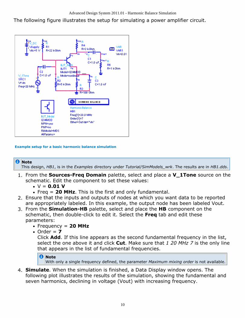
The following figure illustrates the setup for simulating a power amplifier circuit.
Example setup for a basic harmonic balance simulation
NoteThis design, HB1, is in the Examples directory under Tutorial/SimModels_wrk. The results are in HB1.dds.
From the Sources-Freq Domain palette, select and place a V_1Tone source on the1.schematic. Edit the component to set these values:
V = 0.01 VFreq = 20 MHz. This is the first and only fundamental.
Ensure that the inputs and outputs of nodes at which you want data to be reported2.are appropriately labeled. In this example, the output node has been labeled Vout.From the Simulation-HB palette, select and place the HB component on the3.schematic, then double-click to edit it. Select the Freq tab and edit theseparameters:
Frequency = 20 MHzOrder = 7Click Add. If this line appears as the second fundamental frequency in the list,select the one above it and click Cut. Make sure that 1 20 MHz 7 is the only linethat appears in the list of fundamental frequencies.
NoteWith only a single frequency defined, the parameter Maximum mixing order is not available.
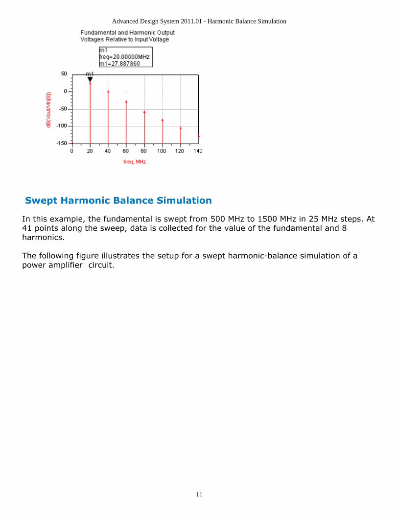
Simulate. When the simulation is finished, a Data Display window opens. The4.following plot illustrates the results of the simulation, showing the fundamental andseven harmonics, declining in voltage (Vout) with increasing frequency.
Advanced Design System 2011.01 - Harmonic Balance Simulation
11
Swept Harmonic Balance Simulation
In this example, the fundamental is swept from 500 MHz to 1500 MHz in 25 MHz steps. At41 points along the sweep, data is collected for the value of the fundamental and 8harmonics.
The following figure illustrates the setup for a swept harmonic-balance simulation of apower amplifier circuit.
Advanced Design System 2011.01 - Harmonic Balance Simulation
12
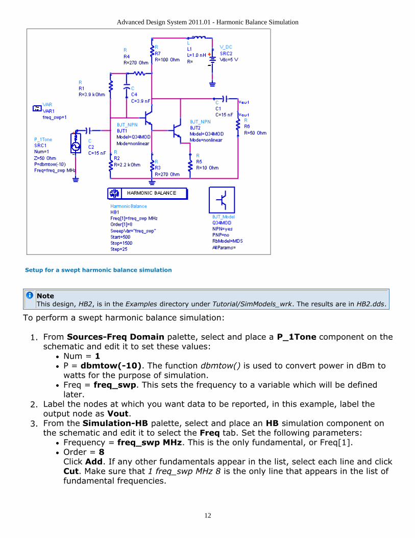
Setup for a swept harmonic balance simulation
NoteThis design, HB2, is in the Examples directory under Tutorial/SimModels_wrk. The results are in HB2.dds.
To perform a swept harmonic balance simulation:
From Sources-Freq Domain palette, select and place a P_1Tone component on the1.schematic and edit it to set these values:
Num = 1P = dbmtow(-10). The function dbmtow() is used to convert power in dBm towatts for the purpose of simulation.Freq = freq_swp. This sets the frequency to a variable which will be definedlater.
Label the nodes at which you want data to be reported, in this example, label the2.output node as Vout.From the Simulation-HB palette, select and place an HB simulation component on3.the schematic and edit it to select the Freq tab. Set the following parameters:
Frequency = freq_swp MHz. This is the only fundamental, or Freq[1].Order = 8Click Add. If any other fundamentals appear in the list, select each line and clickCut. Make sure that 1 freq_swp MHz 8 is the only line that appears in the list offundamental frequencies.
Advanced Design System 2011.01 - Harmonic Balance Simulation
13
NoteEnsure that frequencies are established for all of the frequencies of interest in a design undertest (for example, RF, LO, and IF frequencies). You may want to display them on theschematic to facilitate editing.
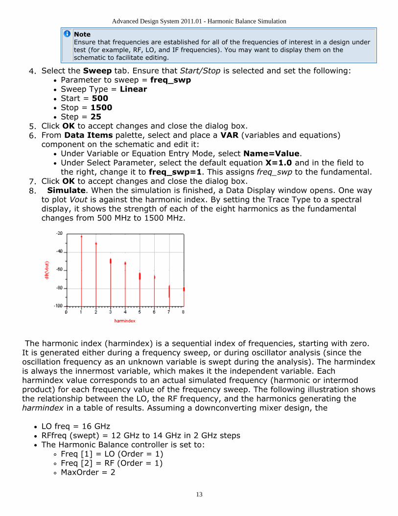
Select the Sweep tab. Ensure that Start/Stop is selected and set the following:4.Parameter to sweep = freq_swpSweep Type = LinearStart = 500Stop = 1500Step = 25
Click OK to accept changes and close the dialog box.5.From Data Items palette, select and place a VAR (variables and equations)6.component on the schematic and edit it:
Under Variable or Equation Entry Mode, select Name=Value.Under Select Parameter, select the default equation X=1.0 and in the field tothe right, change it to freq_swp=1. This assigns freq_swp to the fundamental.
Click OK to accept changes and close the dialog box.7. Simulate. When the simulation is finished, a Data Display window opens. One way8.to plot Vout is against the harmonic index. By setting the Trace Type to a spectraldisplay, it shows the strength of each of the eight harmonics as the fundamentalchanges from 500 MHz to 1500 MHz.
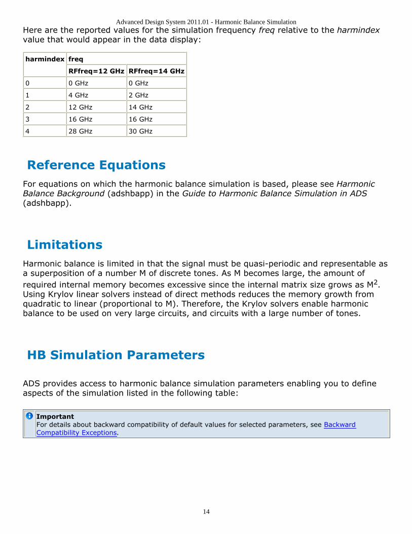
The harmonic index (harmindex) is a sequential index of frequencies, starting with zero.It is generated either during a frequency sweep, or during oscillator analysis (since theoscillation frequency as an unknown variable is swept during the analysis). The harmindexis always the innermost variable, which makes it the independent variable. Eachharmindex value corresponds to an actual simulated frequency (harmonic or intermodproduct) for each frequency value of the frequency sweep. The following illustration showsthe relationship between the LO, the RF frequency, and the harmonics generating theharmindex in a table of results. Assuming a downconverting mixer design, the
LO freq = 16 GHzRFfreq (swept) = 12 GHz to 14 GHz in 2 GHz stepsThe Harmonic Balance controller is set to:
Freq [1] = LO (Order = 1)Freq [2] = RF (Order = 1)MaxOrder = 2
Advanced Design System 2011.01 - Harmonic Balance Simulation
14
Here are the reported values for the simulation frequency freq relative to the harmindexvalue that would appear in the data display:
harmindex freq
RFfreq=12 GHz RFfreq=14 GHz
0 0 GHz 0 GHz
1 4 GHz 2 GHz
2 12 GHz 14 GHz
3 16 GHz 16 GHz
4 28 GHz 30 GHz
Reference EquationsFor equations on which the harmonic balance simulation is based, please see HarmonicBalance Background (adshbapp) in the Guide to Harmonic Balance Simulation in ADS(adshbapp).
LimitationsHarmonic balance is limited in that the signal must be quasi-periodic and representable asa superposition of a number M of discrete tones. As M becomes large, the amount ofrequired internal memory becomes excessive since the internal matrix size grows as M2.Using Krylov linear solvers instead of direct methods reduces the memory growth fromquadratic to linear (proportional to M). Therefore, the Krylov solvers enable harmonicbalance to be used on very large circuits, and circuits with a large number of tones.
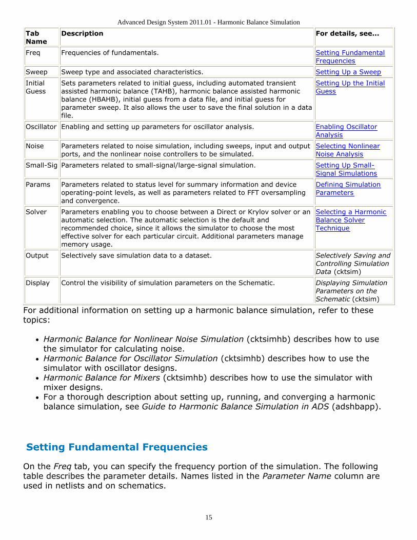
HB Simulation Parameters ADS provides access to harmonic balance simulation parameters enabling you to defineaspects of the simulation listed in the following table:
ImportantFor details about backward compatibility of default values for selected parameters, see BackwardCompatibility Exceptions.
Advanced Design System 2011.01 - Harmonic Balance Simulation
15
TabName
Description For details, see...
Freq Frequencies of fundamentals. Setting FundamentalFrequencies
Sweep Sweep type and associated characteristics. Setting Up a Sweep
InitialGuess
Sets parameters related to initial guess, including automated transientassisted harmonic balance (TAHB), harmonic balance assisted harmonicbalance (HBAHB), initial guess from a data file, and initial guess forparameter sweep. It also allows the user to save the final solution in a datafile.
Setting Up the InitialGuess
Oscillator Enabling and setting up parameters for oscillator analysis. Enabling OscillatorAnalysis
Noise Parameters related to noise simulation, including sweeps, input and outputports, and the nonlinear noise controllers to be simulated.
Selecting NonlinearNoise Analysis
Small-Sig Parameters related to small-signal/large-signal simulation. Setting Up Small-Signal Simulations
Params Parameters related to status level for summary information and deviceoperating-point levels, as well as parameters related to FFT oversamplingand convergence.
Defining SimulationParameters
Solver Parameters enabling you to choose between a Direct or Krylov solver or anautomatic selection. The automatic selection is the default andrecommended choice, since it allows the simulator to choose the mosteffective solver for each particular circuit. Additional parameters managememory usage.
Selecting a HarmonicBalance SolverTechnique
Output Selectively save simulation data to a dataset. Selectively Saving andControlling SimulationData (cktsim)
Display Control the visibility of simulation parameters on the Schematic. Displaying SimulationParameters on theSchematic (cktsim)
For additional information on setting up a harmonic balance simulation, refer to thesetopics:
Harmonic Balance for Nonlinear Noise Simulation (cktsimhb) describes how to usethe simulator for calculating noise.Harmonic Balance for Oscillator Simulation (cktsimhb) describes how to use thesimulator with oscillator designs.Harmonic Balance for Mixers (cktsimhb) describes how to use the simulator withmixer designs.For a thorough description about setting up, running, and converging a harmonicbalance simulation, see Guide to Harmonic Balance Simulation in ADS (adshbapp).
Setting Fundamental Frequencies
On the Freq tab, you can specify the frequency portion of the simulation. The followingtable describes the parameter details. Names listed in the Parameter Name column areused in netlists and on schematics.
Advanced Design System 2011.01 - Harmonic Balance Simulation
16
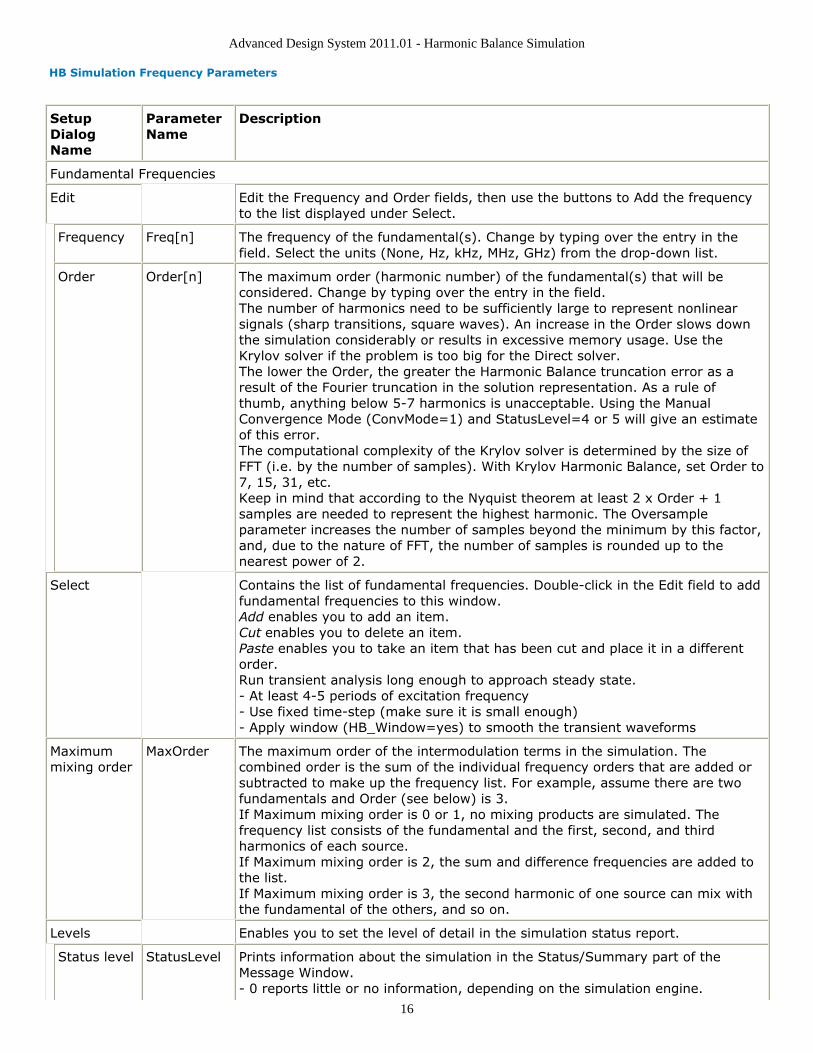
HB Simulation Frequency Parameters
SetupDialogName
ParameterName
Description
Fundamental Frequencies
Edit Edit the Frequency and Order fields, then use the buttons to Add the frequencyto the list displayed under Select.
Frequency Freq[n] The frequency of the fundamental(s). Change by typing over the entry in thefield. Select the units (None, Hz, kHz, MHz, GHz) from the drop-down list.
Order Order[n] The maximum order (harmonic number) of the fundamental(s) that will beconsidered. Change by typing over the entry in the field.The number of harmonics need to be sufficiently large to represent nonlinearsignals (sharp transitions, square waves). An increase in the Order slows downthe simulation considerably or results in excessive memory usage. Use theKrylov solver if the problem is too big for the Direct solver.The lower the Order, the greater the Harmonic Balance truncation error as aresult of the Fourier truncation in the solution representation. As a rule ofthumb, anything below 5-7 harmonics is unacceptable. Using the ManualConvergence Mode (ConvMode=1) and StatusLevel=4 or 5 will give an estimateof this error.The computational complexity of the Krylov solver is determined by the size ofFFT (i.e. by the number of samples). With Krylov Harmonic Balance, set Order to7, 15, 31, etc.Keep in mind that according to the Nyquist theorem at least 2 x Order + 1samples are needed to represent the highest harmonic. The Oversampleparameter increases the number of samples beyond the minimum by this factor,and, due to the nature of FFT, the number of samples is rounded up to thenearest power of 2.
Select Contains the list of fundamental frequencies. Double-click in the Edit field to addfundamental frequencies to this window.Add enables you to add an item.Cut enables you to delete an item.Paste enables you to take an item that has been cut and place it in a differentorder.Run transient analysis long enough to approach steady state.- At least 4-5 periods of excitation frequency- Use fixed time-step (make sure it is small enough)- Apply window (HB_Window=yes) to smooth the transient waveforms
Maximummixing order
MaxOrder The maximum order of the intermodulation terms in the simulation. Thecombined order is the sum of the individual frequency orders that are added orsubtracted to make up the frequency list. For example, assume there are twofundamentals and Order (see below) is 3.If Maximum mixing order is 0 or 1, no mixing products are simulated. Thefrequency list consists of the fundamental and the first, second, and thirdharmonics of each source.If Maximum mixing order is 2, the sum and difference frequencies are added tothe list.If Maximum mixing order is 3, the second harmonic of one source can mix withthe fundamental of the others, and so on.
Levels Enables you to set the level of detail in the simulation status report.
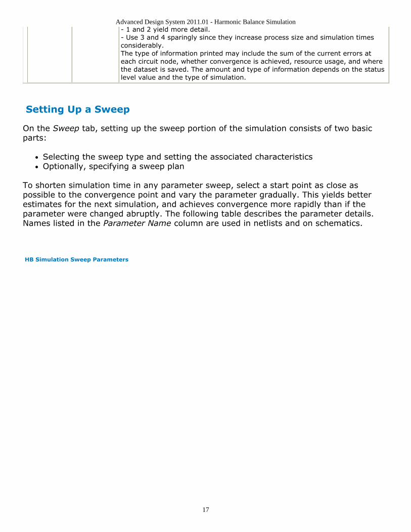
Status level StatusLevel Prints information about the simulation in the Status/Summary part of theMessage Window.- 0 reports little or no information, depending on the simulation engine.
Advanced Design System 2011.01 - Harmonic Balance Simulation
17
- 1 and 2 yield more detail.- Use 3 and 4 sparingly since they increase process size and simulation timesconsiderably.The type of information printed may include the sum of the current errors ateach circuit node, whether convergence is achieved, resource usage, and wherethe dataset is saved. The amount and type of information depends on the statuslevel value and the type of simulation.
Setting Up a Sweep
On the Sweep tab, setting up the sweep portion of the simulation consists of two basicparts:
Selecting the sweep type and setting the associated characteristicsOptionally, specifying a sweep plan
To shorten simulation time in any parameter sweep, select a start point as close aspossible to the convergence point and vary the parameter gradually. This yields betterestimates for the next simulation, and achieves convergence more rapidly than if theparameter were changed abruptly. The following table describes the parameter details.Names listed in the Parameter Name column are used in netlists and on schematics.
HB Simulation Sweep Parameters
Advanced Design System 2011.01 - Harmonic Balance Simulation
18
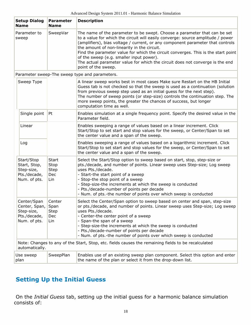
Setup DialogName
ParameterName
Description
Parameter tosweep
SweepVar The name of the parameter to be swept. Choose a parameter that can be setto a value for which the circuit will easily converge: source amplitude / power(amplifiers), bias voltage / current, or any component parameter that controlsthe amount of non-linearity in the circuit.Find the parameter value for which the circuit converges. This is the start pointof the sweep (e.g. smaller input power).The actual parameter value for which the circuit does not converge is the endpoint of the sweep.
Parameter sweep-The sweep type and parameters.
Sweep Type A linear sweep works best in most cases Make sure Restart on the HB InitialGuess tab is not checked so that the sweep is used as a continuation (solutionfrom previous sweep step used as an initial guess for the next step).The number of sweep points (or step-size) controls the continuation step. Themore sweep points, the greater the chances of success, but longercomputation time as well.
Single point Pt Enables simulation at a single frequency point. Specify the desired value in theParameter field.
Linear Enables sweeping a range of values based on a linear increment. ClickStart/Stop to set start and stop values for the sweep, or Center/Span to setthe center value and a span of the sweep.
Log Enables sweeping a range of values based on a logarithmic increment. ClickStart/Stop to set start and stop values for the sweep, or Center/Span to setthe center value and a span of the sweep.
Start/StopStart, Stop,Step-size,Pts./decade,Num. of pts.
StartStopStepDecLin
Select the Start/Stop option to sweep based on start, stop, step-size orpts./decade, and number of points. Linear sweep uses Step-size; Log sweepuses Pts./decade.- Start-the start point of a sweep- Stop-the stop point of a sweep- Step-size-the increments at which the sweep is conducted- Pts./decade-number of points per decade- Num. of pts.-the number of points over which sweep is conducted
Center/SpanCenter, Span,Step-size,Pts./decade,Num. of pts.
CenterSpanStepDecLin
Select the Center/Span option to sweep based on center and span, step-sizeor pts./decade, and number of points. Linear sweep uses Step-size; Log sweepuses Pts./decade.- Center-the center point of a sweep- Span-the span of a sweep- Step-size-the increments at which the sweep is conducted- Pts./decade-number of points per decade- Num. of pts.-the number of points over which sweep is conducted
Note: Changes to any of the Start, Stop, etc. fields causes the remaining fields to be recalculatedautomatically.
Use sweepplan
SweepPlan Enables use of an existing sweep plan component. Select this option and enterthe name of the plan or select it from the drop-down list.
Setting Up the Initial Guess
On the Initial Guess tab, setting up the initial guess for a harmonic balance simulationconsists of:
Advanced Design System 2011.01 - Harmonic Balance Simulation
19
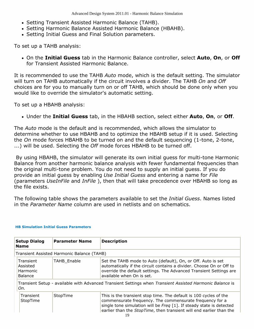
Setting Transient Assisted Harmonic Balance (TAHB).Setting Harmonic Balance Assisted Harmonic Balance (HBAHB).Setting Initial Guess and Final Solution parameters.
To set up a TAHB analysis:
On the Initial Guess tab in the Harmonic Balance controller, select Auto, On, or Offfor Transient Assisted Harmonic Balance.
It is recommended to use the TAHB Auto mode, which is the default setting. The simulatorwill turn on TAHB automatically if the circuit involves a divider. The TAHB On and Offchoices are for you to manually turn on or off TAHB, which should be done only when youwould like to override the simulator's automatic setting.
To set up a HBAHB analysis:
Under the Initial Guess tab, in the HBAHB section, select either Auto, On, or Off.
The Auto mode is the default and is recommended, which allows the simulator todetermine whether to use HBAHB and to optimize the HBAHB setup if it is used. Selectingthe On mode forces HBAHB to be turned on and the default sequencing (1-tone, 2-tone,...) will be used. Selecting the Off mode forces HBAHB to be turned off.
By using HBAHB, the simulator will generate its own initial guess for multi-tone HarmonicBalance from another harmonic balance analysis with fewer fundamental frequencies thanthe original multi-tone problem. You do not need to supply an initial guess. If you doprovide an initial guess by enabling Use Initial Guess and entering a name for File(parameters UseInFile and InFile ), then that will take precedence over HBAHB so long asthe file exists.
The following table shows the parameters available to set the Initial Guess. Names listedin the Parameter Name column are used in netlists and on schematics.
HB Simulation Initial Guess Parameters
Setup DialogName
Parameter Name Description
Transient Assisted Harmonic Balance (TAHB)
TransientAssistedHarmonicBalance
TAHB_Enable Set the TAHB mode to Auto (default), On, or Off. Auto is setautomatically if the circuit contains a divider. Choose On or Off tooverride the default settings. The Advanced Transient Settings areavailable when On is set.
Transient Setup - available with Advanced Transient Settings when Transient Assisted Harmonic Balance isOn.
TransientStopTime
StopTime This is the transient stop time. The default is 100 cycles of thecommensurate frequency. The commensurate frequency for asingle tone simulation will be Freq [1]. If steady state is detectedearlier than the StopTime, then transient will end earlier than the
Advanced Design System 2011.01 - Harmonic Balance Simulation
20
StopTime.
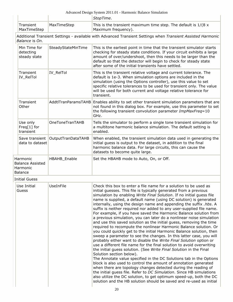
TransientMaxTimeStep
MaxTimeStep This is the transient maximum time step. The default is 1/(8 xMaximum frequency).
Additional Transient Settings - available with Advanced Transient Settings when Transient Assisted HarmonicBalance is On.
Min Time fordetectingsteady state
SteadyStateMinTime This is the earliest point in time that the transient simulator startschecking for steady state conditions. If your circuit exhibits a largeamount of over/undershoot, then this needs to be larger than thedefault so that the detector will begin to check for steady stateafter some of the initial transients have settled.
TransientIV_RelTol
IV_RelTol This is the transient relative voltage and current tolerance. Thedefault is 1e-3. When simulation options are included in thesimulation (using the Options controller), use this value to setspecific relative tolerances to be used for transient only. The valuewill be used for both current and voltage relative tolerance fortransient.
TransientOther
AddtlTranParamsTAHB Enables ability to set other transient simulation parameters that arenot found in this dialog box. For example, use this parameter to setthe following transient convolution parameter ImpMaxFreq=10GHz.
Use onlyFreq[1] fortransient
OneToneTranTAHB Tells the simulator to perform a single tone transient simulation fora multitone harmonic balance simulation. The default setting isenabled.
Save transientdata to dataset
OutputTranDataTAHB When enabled, the transient simulation data used in generating theinitial guess is output to the dataset, in addition to the finalharmonic balance data. For large circuits, this can cause thedatasets to become quite large.
HarmonicBalance AssistedHarmonicBalance
HBAHB_Enable Set the HBAHB mode to Auto, On, or Off.
Initial Guess
Use InitialGuess
UseInFile Check this box to enter a file name for a solution to be used asinitial guesses. This file is typically generated from a previoussimulation by enabling Write Final Solution. If no initial guess filename is supplied, a default name (using DC solution) is generatedinternally, using the design name and appending the suffix .hbs. Asuffix is neither required nor added to any user-supplied file name.For example, if you have saved the Harmonic Balance solution froma previous simulation, you can later do a nonlinear noise simulationand use this saved solution as the initial guess, removing the timerequired to recompute the nonlinear Harmonic Balance solution. Oryou could quickly get to the initial Harmonic Balance solution, thensweep a parameter to see the changes. In this latter case, you willprobably either want to disable the Write Final Solution option oruse a different file name for the final solution to avoid overwritingthe initial guess solution. (See Write Final Solution in the FinalSolution section below).The Annotate value specified in the DC Solutions tab in the Optionsblock is also used to control the amount of annotation generatedwhen there are topology changes detected during the reading ofthe initial guess file. Refer to DC Simulation. Since HB simulationsalso utilize the DC solution, to get optimum speed-up, both the DCsolution and the HB solution should be saved and re-used as initial
Advanced Design System 2011.01 - Harmonic Balance Simulation
21
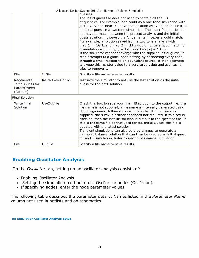
guesses.The initial guess file does not need to contain all the HBfrequencies. For example, one could do a one-tone simulation withjust a very nonlinear LO, save that solution away and then use it asan initial guess in a two tone simulation. The exact frequencies donot have to match between the present analysis and the initialguess solution. However, the fundamental indexes should match.For example, a solution saved from a two tone analysis withFreq[1] = 1GHz and Freq[2]= 1kHz would not be a good match fora simulation with Freq[1] = 1kHz and Freq[2] = 1 GHz.If the simulator cannot converge with the supplied initial guess, itthen attempts to a global node-setting by connecting every nodethrough a small resistor to an equivalent source. It then attemptsto sweep this resistor value to a very large value and eventuallytries to remove it.
File InFile Specify a file name to save results.
RegenerateInitial Guess forParamSweep(Restart)
Restart=yes or no Instructs the simulator to not use the last solution as the initialguess for the next solution.
Final Solution
Write FinalSolution
UseOutFile Check this box to save your final HB solution to the output file. If afile name is not supplied, a file name is internally generated usingthe design name, followed by an .hbs suffix. If a file name issupplied, the suffix is neither appended nor required. If this box ischecked, then the last HB solution is put out to the specified file. Ifthis is the same file as that used for the Initial Guess, this file isupdated with the latest solution.Transient simulations can also be programmed to generate aharmonic balance solution that can then be used as an initial guessfor an HB simulation. Refer to Harmonic Balance Simulation.
File OutFile Specify a file name to save results.
Enabling Oscillator Analysis
On the Oscillator tab, setting up an oscillator analysis consists of:
Enabling Oscillator Analysis. Setting the simulation method to use OscPort or nodes (OscProbe).If specifying nodes, enter the node parameter values.
The following table describes the parameter details. Names listed in the Parameter Namecolumn are used in netlists and on schematics.
HB Simulation Oscillator Analysis Setup
Advanced Design System 2011.01 - Harmonic Balance Simulation
22
Setup DialogName
ParameterName
Description
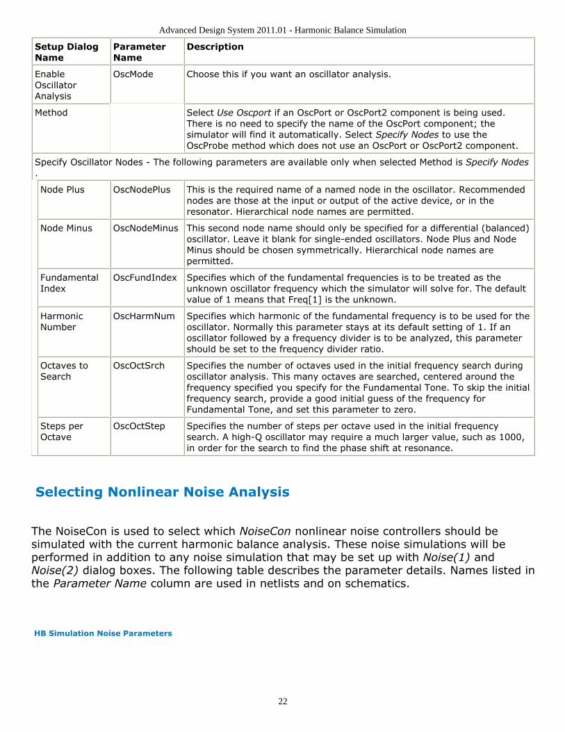
EnableOscillatorAnalysis
OscMode Choose this if you want an oscillator analysis.
Method Select Use Oscport if an OscPort or OscPort2 component is being used.There is no need to specify the name of the OscPort component; thesimulator will find it automatically. Select Specify Nodes to use theOscProbe method which does not use an OscPort or OscPort2 component.
Specify Oscillator Nodes - The following parameters are available only when selected Method is Specify Nodes.
Node Plus OscNodePlus This is the required name of a named node in the oscillator. Recommendednodes are those at the input or output of the active device, or in theresonator. Hierarchical node names are permitted.
Node Minus OscNodeMinus This second node name should only be specified for a differential (balanced)oscillator. Leave it blank for single-ended oscillators. Node Plus and NodeMinus should be chosen symmetrically. Hierarchical node names arepermitted.
FundamentalIndex
OscFundIndex Specifies which of the fundamental frequencies is to be treated as theunknown oscillator frequency which the simulator will solve for. The defaultvalue of 1 means that Freq[1] is the unknown.
HarmonicNumber
OscHarmNum Specifies which harmonic of the fundamental frequency is to be used for theoscillator. Normally this parameter stays at its default setting of 1. If anoscillator followed by a frequency divider is to be analyzed, this parametershould be set to the frequency divider ratio.
Octaves toSearch
OscOctSrch Specifies the number of octaves used in the initial frequency search duringoscillator analysis. This many octaves are searched, centered around thefrequency specified you specify for the Fundamental Tone. To skip the initialfrequency search, provide a good initial guess of the frequency forFundamental Tone, and set this parameter to zero.
Steps perOctave
OscOctStep Specifies the number of steps per octave used in the initial frequencysearch. A high-Q oscillator may require a much larger value, such as 1000,in order for the search to find the phase shift at resonance.
Selecting Nonlinear Noise Analysis
The NoiseCon is used to select which NoiseCon nonlinear noise controllers should besimulated with the current harmonic balance analysis. These noise simulations will beperformed in addition to any noise simulation that may be set up with Noise(1) andNoise(2) dialog boxes. The following table describes the parameter details. Names listed inthe Parameter Name column are used in netlists and on schematics.
HB Simulation Noise Parameters
Advanced Design System 2011.01 - Harmonic Balance Simulation
23
SetupDialogName
ParameterName
Description
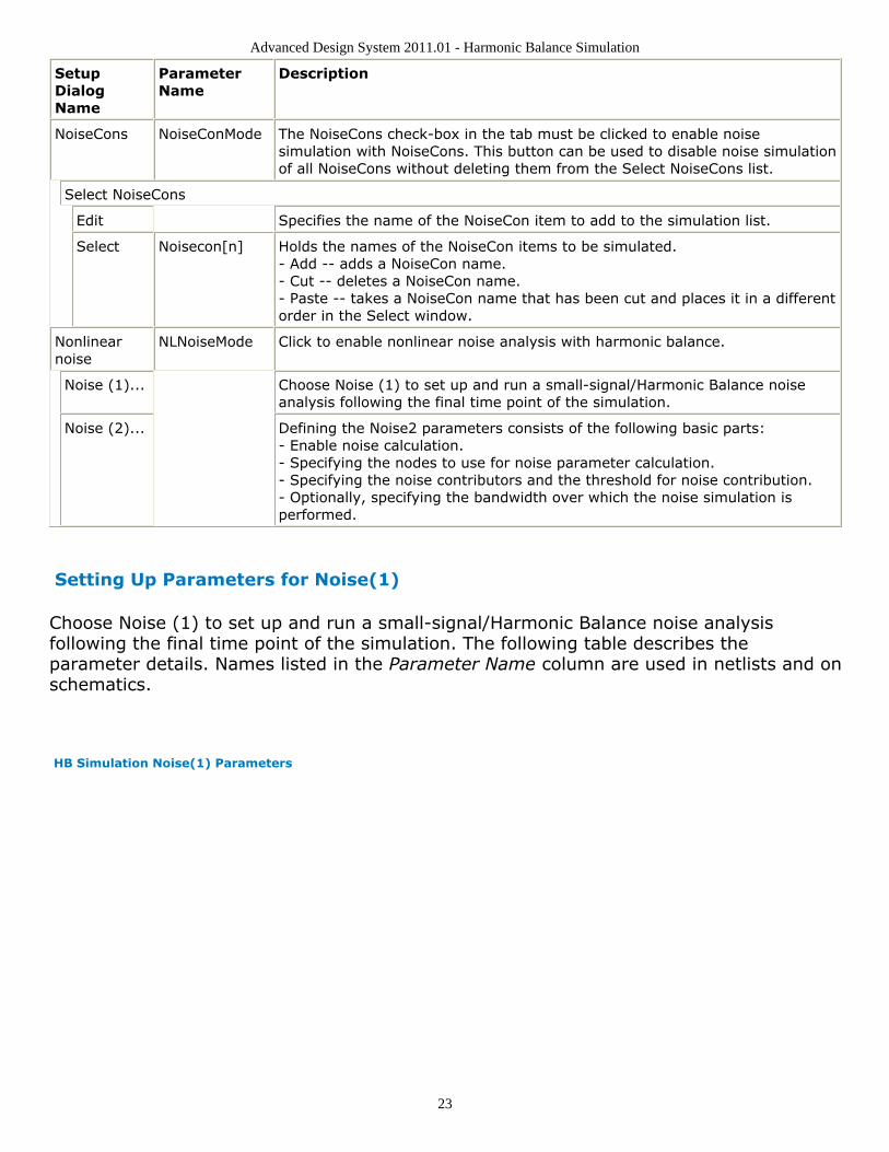
NoiseCons NoiseConMode The NoiseCons check-box in the tab must be clicked to enable noisesimulation with NoiseCons. This button can be used to disable noise simulationof all NoiseCons without deleting them from the Select NoiseCons list.
Select NoiseCons
Edit Specifies the name of the NoiseCon item to add to the simulation list.
Select Noisecon[n] Holds the names of the NoiseCon items to be simulated.- Add -- adds a NoiseCon name.- Cut -- deletes a NoiseCon name.- Paste -- takes a NoiseCon name that has been cut and places it in a differentorder in the Select window.
Nonlinearnoise
NLNoiseMode Click to enable nonlinear noise analysis with harmonic balance.
Noise (1)... Choose Noise (1) to set up and run a small-signal/Harmonic Balance noiseanalysis following the final time point of the simulation.
Noise (2)... Defining the Noise2 parameters consists of the following basic parts:- Enable noise calculation.- Specifying the nodes to use for noise parameter calculation.- Specifying the noise contributors and the threshold for noise contribution.- Optionally, specifying the bandwidth over which the noise simulation isperformed.
Setting Up Parameters for Noise(1)
Choose Noise (1) to set up and run a small-signal/Harmonic Balance noise analysisfollowing the final time point of the simulation. The following table describes theparameter details. Names listed in the Parameter Name column are used in netlists and onschematics.
HB Simulation Noise(1) Parameters
Advanced Design System 2011.01 - Harmonic Balance Simulation
24
Setup DialogName
ParameterName
Description
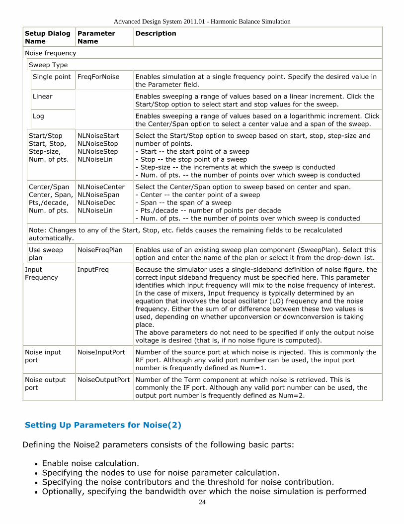
Noise frequency
Sweep Type
Single point FreqForNoise Enables simulation at a single frequency point. Specify the desired value inthe Parameter field.
Linear Enables sweeping a range of values based on a linear increment. Click theStart/Stop option to select start and stop values for the sweep.
Log Enables sweeping a range of values based on a logarithmic increment. Clickthe Center/Span option to select a center value and a span of the sweep.
Start/StopStart, Stop,Step-size,Num. of pts.
NLNoiseStartNLNoiseStopNLNoiseStepNLNoiseLin
Select the Start/Stop option to sweep based on start, stop, step-size andnumber of points.- Start -- the start point of a sweep- Stop -- the stop point of a sweep- Step-size -- the increments at which the sweep is conducted- Num. of pts. -- the number of points over which sweep is conducted
Center/SpanCenter, Span,Pts,/decade,Num. of pts.
NLNoiseCenterNLNoiseSpanNLNoiseDecNLNoiseLin
Select the Center/Span option to sweep based on center and span.- Center -- the center point of a sweep- Span -- the span of a sweep- Pts./decade -- number of points per decade- Num. of pts. -- the number of points over which sweep is conducted
Note: Changes to any of the Start, Stop, etc. fields causes the remaining fields to be recalculatedautomatically.
Use sweepplan
NoiseFreqPlan Enables use of an existing sweep plan component (SweepPlan). Select thisoption and enter the name of the plan or select it from the drop-down list.
InputFrequency
InputFreq Because the simulator uses a single-sideband definition of noise figure, thecorrect input sideband frequency must be specified here. This parameteridentifies which input frequency will mix to the noise frequency of interest.In the case of mixers, Input frequency is typically determined by anequation that involves the local oscillator (LO) frequency and the noisefrequency. Either the sum of or difference between these two values isused, depending on whether upconversion or downconversion is takingplace.The above parameters do not need to be specified if only the output noisevoltage is desired (that is, if no noise figure is computed).
Noise inputport
NoiseInputPort Number of the source port at which noise is injected. This is commonly theRF port. Although any valid port number can be used, the input portnumber is frequently defined as Num=1.
Noise outputport
NoiseOutputPort Number of the Term component at which noise is retrieved. This iscommonly the IF port. Although any valid port number can be used, theoutput port number is frequently defined as Num=2.
Setting Up Parameters for Noise(2)
Defining the Noise2 parameters consists of the following basic parts:
Enable noise calculation.Specifying the nodes to use for noise parameter calculation.Specifying the noise contributors and the threshold for noise contribution.Optionally, specifying the bandwidth over which the noise simulation is performed
Advanced Design System 2011.01 - Harmonic Balance Simulation
25
The following table describes the parameter details. Names listed in the Parameter Namecolumn are used in netlists and on schematics.
HB Simulation Noise(2) Parameters
SetupDialogName
Parameter Name Description
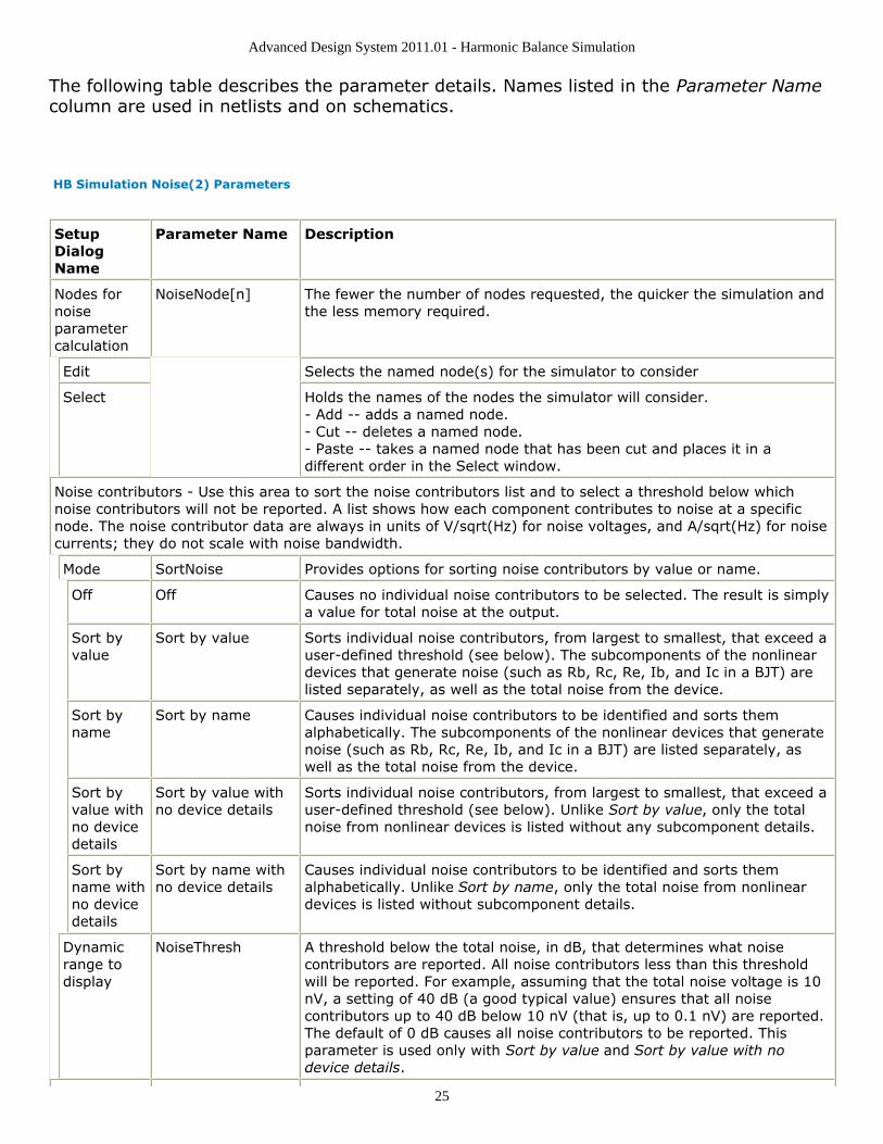
Nodes fornoiseparametercalculation
NoiseNode[n] The fewer the number of nodes requested, the quicker the simulation andthe less memory required.
Edit Selects the named node(s) for the simulator to consider
Select Holds the names of the nodes the simulator will consider.- Add -- adds a named node.- Cut -- deletes a named node.- Paste -- takes a named node that has been cut and places it in adifferent order in the Select window.
Noise contributors - Use this area to sort the noise contributors list and to select a threshold below whichnoise contributors will not be reported. A list shows how each component contributes to noise at a specificnode. The noise contributor data are always in units of V/sqrt(Hz) for noise voltages, and A/sqrt(Hz) for noisecurrents; they do not scale with noise bandwidth.
Mode SortNoise Provides options for sorting noise contributors by value or name.
Off Off Causes no individual noise contributors to be selected. The result is simplya value for total noise at the output.
Sort byvalue
Sort by value Sorts individual noise contributors, from largest to smallest, that exceed auser-defined threshold (see below). The subcomponents of the nonlineardevices that generate noise (such as Rb, Rc, Re, Ib, and Ic in a BJT) arelisted separately, as well as the total noise from the device.
Sort byname
Sort by name Causes individual noise contributors to be identified and sorts themalphabetically. The subcomponents of the nonlinear devices that generatenoise (such as Rb, Rc, Re, Ib, and Ic in a BJT) are listed separately, aswell as the total noise from the device.
Sort byvalue withno devicedetails
Sort by value withno device details
Sorts individual noise contributors, from largest to smallest, that exceed auser-defined threshold (see below). Unlike Sort by value, only the totalnoise from nonlinear devices is listed without any subcomponent details.
Sort byname withno devicedetails
Sort by name withno device details
Causes individual noise contributors to be identified and sorts themalphabetically. Unlike Sort by name, only the total noise from nonlineardevices is listed without subcomponent details.
Dynamicrange todisplay
NoiseThresh A threshold below the total noise, in dB, that determines what noisecontributors are reported. All noise contributors less than this thresholdwill be reported. For example, assuming that the total noise voltage is 10nV, a setting of 40 dB (a good typical value) ensures that all noisecontributors up to 40 dB below 10 nV (that is, up to 0.1 nV) are reported.The default of 0 dB causes all noise contributors to be reported. Thisparameter is used only with Sort by value and Sort by value with nodevice details.
Advanced Design System 2011.01 - Harmonic Balance Simulation
26
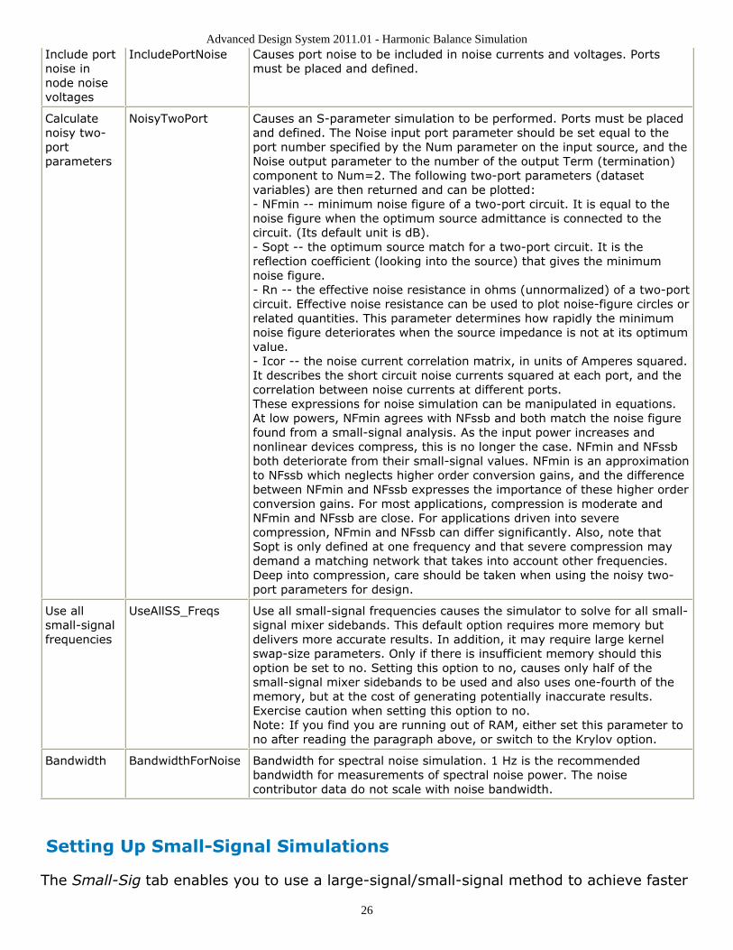
Include portnoise innode noisevoltages
IncludePortNoise Causes port noise to be included in noise currents and voltages. Portsmust be placed and defined.
Calculatenoisy two-portparameters
NoisyTwoPort Causes an S-parameter simulation to be performed. Ports must be placedand defined. The Noise input port parameter should be set equal to theport number specified by the Num parameter on the input source, and theNoise output parameter to the number of the output Term (termination)component to Num=2. The following two-port parameters (datasetvariables) are then returned and can be plotted:- NFmin -- minimum noise figure of a two-port circuit. It is equal to thenoise figure when the optimum source admittance is connected to thecircuit. (Its default unit is dB).- Sopt -- the optimum source match for a two-port circuit. It is thereflection coefficient (looking into the source) that gives the minimumnoise figure.- Rn -- the effective noise resistance in ohms (unnormalized) of a two-portcircuit. Effective noise resistance can be used to plot noise-figure circles orrelated quantities. This parameter determines how rapidly the minimumnoise figure deteriorates when the source impedance is not at its optimumvalue.- Icor -- the noise current correlation matrix, in units of Amperes squared.It describes the short circuit noise currents squared at each port, and thecorrelation between noise currents at different ports.These expressions for noise simulation can be manipulated in equations.At low powers, NFmin agrees with NFssb and both match the noise figurefound from a small-signal analysis. As the input power increases andnonlinear devices compress, this is no longer the case. NFmin and NFssbboth deteriorate from their small-signal values. NFmin is an approximationto NFssb which neglects higher order conversion gains, and the differencebetween NFmin and NFssb expresses the importance of these higher orderconversion gains. For most applications, compression is moderate andNFmin and NFssb are close. For applications driven into severecompression, NFmin and NFssb can differ significantly. Also, note thatSopt is only defined at one frequency and that severe compression maydemand a matching network that takes into account other frequencies.Deep into compression, care should be taken when using the noisy two-port parameters for design.
Use allsmall-signalfrequencies
UseAllSS_Freqs Use all small-signal frequencies causes the simulator to solve for all small-signal mixer sidebands. This default option requires more memory butdelivers more accurate results. In addition, it may require large kernelswap-size parameters. Only if there is insufficient memory should thisoption be set to no. Setting this option to no, causes only half of thesmall-signal mixer sidebands to be used and also uses one-fourth of thememory, but at the cost of generating potentially inaccurate results.Exercise caution when setting this option to no.Note: If you find you are running out of RAM, either set this parameter tono after reading the paragraph above, or switch to the Krylov option.
Bandwidth BandwidthForNoise Bandwidth for spectral noise simulation. 1 Hz is the recommendedbandwidth for measurements of spectral noise power. The noisecontributor data do not scale with noise bandwidth.
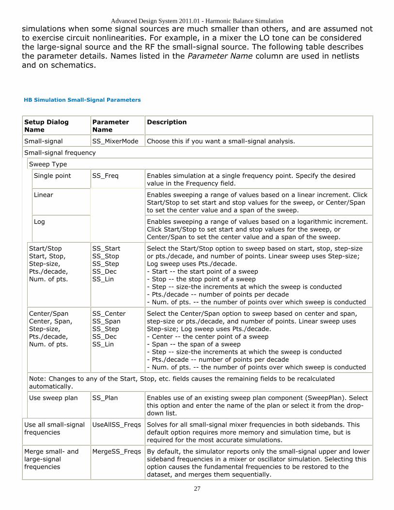
Setting Up Small-Signal Simulations
The Small-Sig tab enables you to use a large-signal/small-signal method to achieve faster
Advanced Design System 2011.01 - Harmonic Balance Simulation
27
simulations when some signal sources are much smaller than others, and are assumed notto exercise circuit nonlinearities. For example, in a mixer the LO tone can be consideredthe large-signal source and the RF the small-signal source. The following table describesthe parameter details. Names listed in the Parameter Name column are used in netlistsand on schematics.
HB Simulation Small-Signal Parameters
Setup DialogName
ParameterName
Description
Small-signal SS_MixerMode Choose this if you want a small-signal analysis.
Small-signal frequency
Sweep Type
Single point SS_Freq Enables simulation at a single frequency point. Specify the desiredvalue in the Frequency field.
Linear Enables sweeping a range of values based on a linear increment. ClickStart/Stop to set start and stop values for the sweep, or Center/Spanto set the center value and a span of the sweep.
Log Enables sweeping a range of values based on a logarithmic increment.Click Start/Stop to set start and stop values for the sweep, orCenter/Span to set the center value and a span of the sweep.
Start/StopStart, Stop,Step-size,Pts./decade,Num. of pts.
SS_StartSS_StopSS_StepSS_DecSS_Lin
Select the Start/Stop option to sweep based on start, stop, step-sizeor pts./decade, and number of points. Linear sweep uses Step-size;Log sweep uses Pts./decade.- Start -- the start point of a sweep- Stop -- the stop point of a sweep- Step -- size-the increments at which the sweep is conducted- Pts./decade -- number of points per decade- Num. of pts. -- the number of points over which sweep is conducted
Center/SpanCenter, Span,Step-size,Pts./decade,Num. of pts.
SS_CenterSS_SpanSS_StepSS_DecSS_Lin
Select the Center/Span option to sweep based on center and span,step-size or pts./decade, and number of points. Linear sweep usesStep-size; Log sweep uses Pts./decade.- Center -- the center point of a sweep- Span -- the span of a sweep- Step -- size-the increments at which the sweep is conducted- Pts./decade -- number of points per decade- Num. of pts. -- the number of points over which sweep is conducted
Note: Changes to any of the Start, Stop, etc. fields causes the remaining fields to be recalculatedautomatically.
Use sweep plan SS_Plan Enables use of an existing sweep plan component (SweepPlan). Selectthis option and enter the name of the plan or select it from the drop-down list.
Use all small-signalfrequencies
UseAllSS_Freqs Solves for all small-signal mixer frequencies in both sidebands. Thisdefault option requires more memory and simulation time, but isrequired for the most accurate simulations.
Merge small- andlarge-signalfrequencies
MergeSS_Freqs By default, the simulator reports only the small-signal upper and lowersideband frequencies in a mixer or oscillator simulation. Selecting thisoption causes the fundamental frequencies to be restored to thedataset, and merges them sequentially.
Advanced Design System 2011.01 - Harmonic Balance Simulation
28
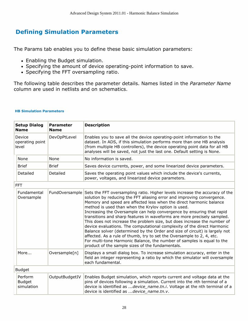
Defining Simulation Parameters
The Params tab enables you to define these basic simulation parameters:
Enabling the Budget simulation. Specifying the amount of device operating-point information to save.Specifying the FFT oversampling ratio.
The following table describes the parameter details. Names listed in the Parameter Namecolumn are used in netlists and on schematics.
HB Simulation Parameters
Setup DialogName
ParameterName
Description
Deviceoperating pointlevel
DevOpPtLevel Enables you to save all the device operating-point information to thedataset. In ADS, if this simulation performs more than one HB analysis(from multiple HB controllers), the device operating point data for all HBanalyses will be saved, not just the last one. Default setting is None.
None None No information is saved.
Brief Brief Saves device currents, power, and some linearized device parameters.
Detailed Detailed Saves the operating point values which include the device's currents,power, voltages, and linearized device parameters.
FFT
FundamentalOversample
FundOversample Sets the FFT oversampling ratio. Higher levels increase the accuracy of thesolution by reducing the FFT aliasing error and improving convergence.Memory and speed are affected less when the direct harmonic balancemethod is used than when the Krylov option is used.Increasing the Oversample can help convergence by ensuring that rapidtransitions and sharp features in waveforms are more precisely sampled.This does not increase the problem size, but does increase the number ofdevice evaluations. The computational complexity of the direct HarmonicBalance solver (determined by the Order and size of circuit) is largely notaffected. As a rule of thumb, try to set the Oversample to 2, 4, etc.For multi-tone Harmonic Balance, the number of samples is equal to theproduct of the sample sizes of the fundamentals.
More... Oversample[n] Displays a small dialog box. To increase simulation accuracy, enter in thefield an integer representing a ratio by which the simulator will oversampleeach fundamental.
Budget
PerformBudgetsimulation
OutputBudgetIV Enables Budget simulation, which reports current and voltage data at thepins of devices following a simulation. Current into the nth terminal of adevice is identified as ...device_name.tn.i. Voltage at the nth terminal of adevice is identified as ...device_name.tn.v.
Advanced Design System 2011.01 - Harmonic Balance Simulation
29
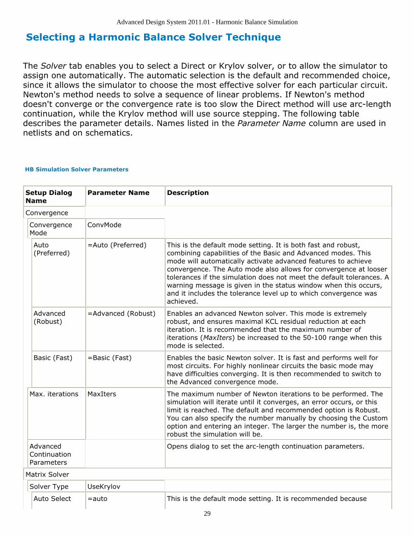
Selecting a Harmonic Balance Solver Technique
The Solver tab enables you to select a Direct or Krylov solver, or to allow the simulator toassign one automatically. The automatic selection is the default and recommended choice,since it allows the simulator to choose the most effective solver for each particular circuit.Newton's method needs to solve a sequence of linear problems. If Newton's methoddoesn't converge or the convergence rate is too slow the Direct method will use arc-lengthcontinuation, while the Krylov method will use source stepping. The following tabledescribes the parameter details. Names listed in the Parameter Name column are used innetlists and on schematics.
HB Simulation Solver Parameters
Setup DialogName
Parameter Name Description
Convergence
ConvergenceMode
ConvMode
Auto(Preferred)
=Auto (Preferred) This is the default mode setting. It is both fast and robust,combining capabilities of the Basic and Advanced modes. Thismode will automatically activate advanced features to achieveconvergence. The Auto mode also allows for convergence at loosertolerances if the simulation does not meet the default tolerances. Awarning message is given in the status window when this occurs,and it includes the tolerance level up to which convergence wasachieved.
Advanced(Robust)
=Advanced (Robust) Enables an advanced Newton solver. This mode is extremelyrobust, and ensures maximal KCL residual reduction at eachiteration. It is recommended that the maximum number ofiterations (MaxIters) be increased to the 50-100 range when thismode is selected.
Basic (Fast) =Basic (Fast) Enables the basic Newton solver. It is fast and performs well formost circuits. For highly nonlinear circuits the basic mode mayhave difficulties converging. It is then recommended to switch tothe Advanced convergence mode.
Max. iterations MaxIters The maximum number of Newton iterations to be performed. Thesimulation will iterate until it converges, an error occurs, or thislimit is reached. The default and recommended option is Robust.You can also specify the number manually by choosing the Customoption and entering an integer. The larger the number is, the morerobust the simulation will be.
AdvancedContinuationParameters
Opens dialog to set the arc-length continuation parameters.
Matrix Solver
Solver Type UseKrylov
Auto Select =auto This is the default mode setting. It is recommended because
Advanced Design System 2011.01 - Harmonic Balance Simulation
30
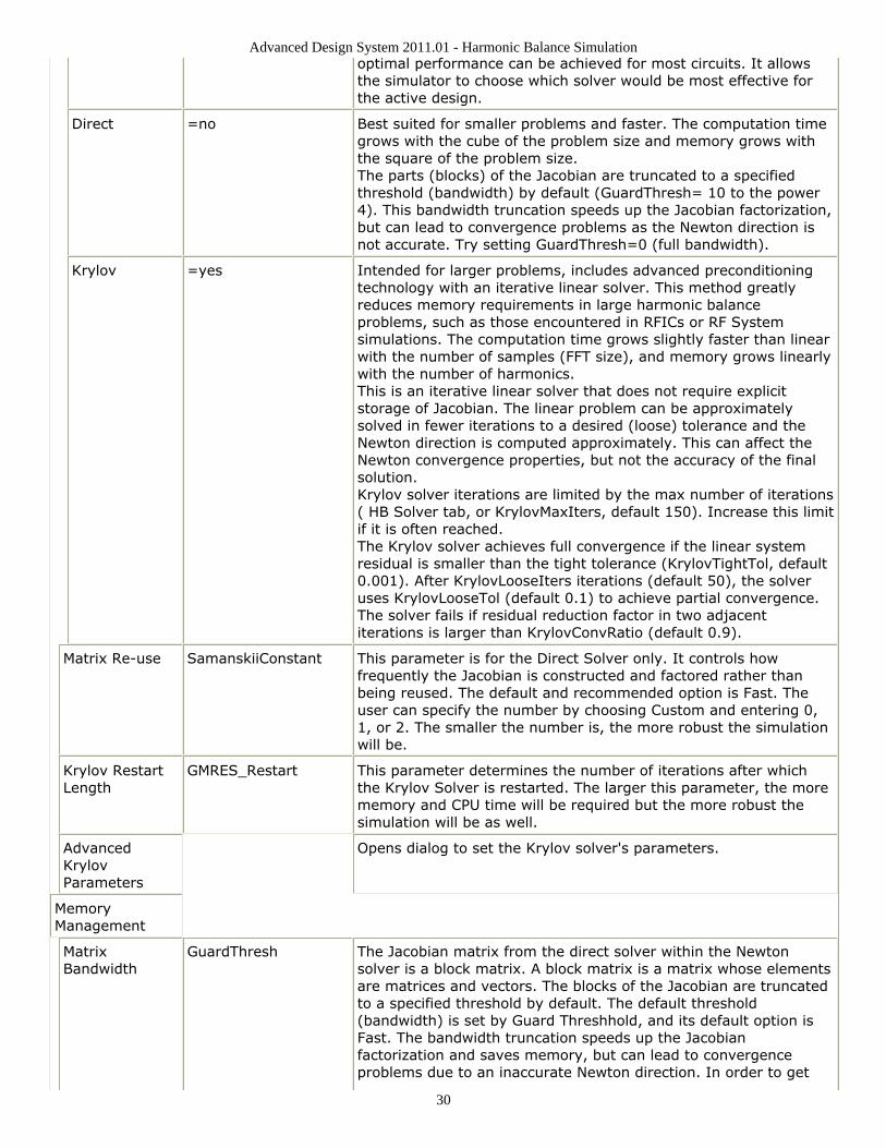
optimal performance can be achieved for most circuits. It allowsthe simulator to choose which solver would be most effective forthe active design.
Direct =no Best suited for smaller problems and faster. The computation timegrows with the cube of the problem size and memory grows withthe square of the problem size.The parts (blocks) of the Jacobian are truncated to a specifiedthreshold (bandwidth) by default (GuardThresh= 10 to the power4). This bandwidth truncation speeds up the Jacobian factorization,but can lead to convergence problems as the Newton direction isnot accurate. Try setting GuardThresh=0 (full bandwidth).
Krylov =yes Intended for larger problems, includes advanced preconditioningtechnology with an iterative linear solver. This method greatlyreduces memory requirements in large harmonic balanceproblems, such as those encountered in RFICs or RF Systemsimulations. The computation time grows slightly faster than linearwith the number of samples (FFT size), and memory grows linearlywith the number of harmonics.This is an iterative linear solver that does not require explicitstorage of Jacobian. The linear problem can be approximatelysolved in fewer iterations to a desired (loose) tolerance and theNewton direction is computed approximately. This can affect theNewton convergence properties, but not the accuracy of the finalsolution.Krylov solver iterations are limited by the max number of iterations( HB Solver tab, or KrylovMaxIters, default 150). Increase this limitif it is often reached.The Krylov solver achieves full convergence if the linear systemresidual is smaller than the tight tolerance (KrylovTightTol, default0.001). After KrylovLooseIters iterations (default 50), the solveruses KrylovLooseTol (default 0.1) to achieve partial convergence.The solver fails if residual reduction factor in two adjacentiterations is larger than KrylovConvRatio (default 0.9).
Matrix Re-use SamanskiiConstant This parameter is for the Direct Solver only. It controls howfrequently the Jacobian is constructed and factored rather thanbeing reused. The default and recommended option is Fast. Theuser can specify the number by choosing Custom and entering 0,1, or 2. The smaller the number is, the more robust the simulationwill be.
Krylov RestartLength
GMRES_Restart This parameter determines the number of iterations after whichthe Krylov Solver is restarted. The larger this parameter, the morememory and CPU time will be required but the more robust thesimulation will be as well.
AdvancedKrylovParameters
Opens dialog to set the Krylov solver's parameters.
MemoryManagement
MatrixBandwidth
GuardThresh The Jacobian matrix from the direct solver within the Newtonsolver is a block matrix. A block matrix is a matrix whose elementsare matrices and vectors. The blocks of the Jacobian are truncatedto a specified threshold by default. The default threshold(bandwidth) is set by Guard Threshhold, and its default option isFast. The bandwidth truncation speeds up the Jacobianfactorization and saves memory, but can lead to convergenceproblems due to an inaccurate Newton direction. In order to get
Advanced Design System 2011.01 - Harmonic Balance Simulation
31
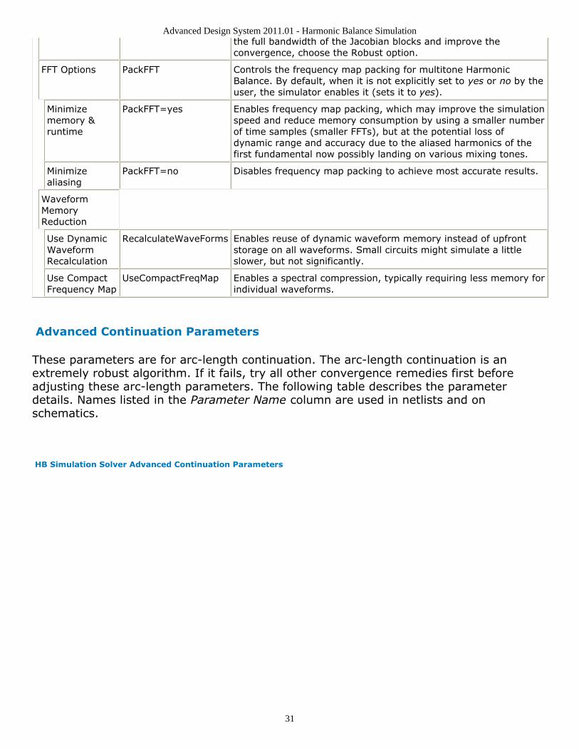
the full bandwidth of the Jacobian blocks and improve theconvergence, choose the Robust option.
FFT Options PackFFT Controls the frequency map packing for multitone HarmonicBalance. By default, when it is not explicitly set to yes or no by theuser, the simulator enables it (sets it to yes).
Minimizememory &runtime
PackFFT=yes Enables frequency map packing, which may improve the simulationspeed and reduce memory consumption by using a smaller numberof time samples (smaller FFTs), but at the potential loss ofdynamic range and accuracy due to the aliased harmonics of thefirst fundamental now possibly landing on various mixing tones.
Minimizealiasing
PackFFT=no Disables frequency map packing to achieve most accurate results.
WaveformMemoryReduction
Use DynamicWaveformRecalculation
RecalculateWaveForms Enables reuse of dynamic waveform memory instead of upfrontstorage on all waveforms. Small circuits might simulate a littleslower, but not significantly.
Use CompactFrequency Map
UseCompactFreqMap Enables a spectral compression, typically requiring less memory forindividual waveforms.
Advanced Continuation Parameters
These parameters are for arc-length continuation. The arc-length continuation is anextremely robust algorithm. If it fails, try all other convergence remedies first beforeadjusting these arc-length parameters. The following table describes the parameterdetails. Names listed in the Parameter Name column are used in netlists and onschematics.
HB Simulation Solver Advanced Continuation Parameters
Advanced Design System 2011.01 - Harmonic Balance Simulation
32
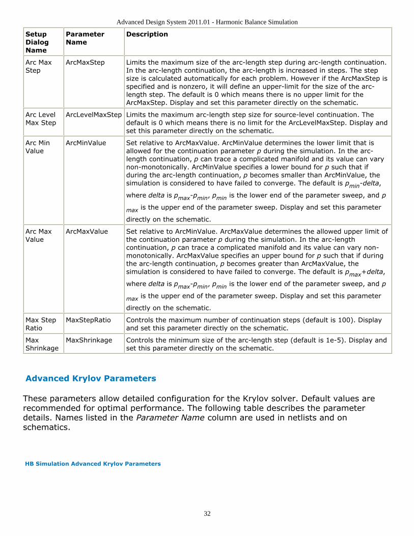
SetupDialogName
ParameterName
Description
Arc MaxStep
ArcMaxStep Limits the maximum size of the arc-length step during arc-length continuation.In the arc-length continuation, the arc-length is increased in steps. The stepsize is calculated automatically for each problem. However if the ArcMaxStep isspecified and is nonzero, it will define an upper-limit for the size of the arc-length step. The default is 0 which means there is no upper limit for theArcMaxStep. Display and set this parameter directly on the schematic.
Arc LevelMax Step
ArcLevelMaxStep Limits the maximum arc-length step size for source-level continuation. Thedefault is 0 which means there is no limit for the ArcLevelMaxStep. Display andset this parameter directly on the schematic.
Arc MinValue
ArcMinValue Set relative to ArcMaxValue. ArcMinValue determines the lower limit that isallowed for the continuation parameter p during the simulation. In the arc-length continuation, p can trace a complicated manifold and its value can varynon-monotonically. ArcMinValue specifies a lower bound for p such that ifduring the arc-length continuation, p becomes smaller than ArcMinValue, thesimulation is considered to have failed to converge. The default is pmin-delta,
where delta is pmax-pmin, pmin is the lower end of the parameter sweep, and p
max is the upper end of the parameter sweep. Display and set this parameter
directly on the schematic.
Arc MaxValue
ArcMaxValue Set relative to ArcMinValue. ArcMaxValue determines the allowed upper limit ofthe continuation parameter p during the simulation. In the arc-lengthcontinuation, p can trace a complicated manifold and its value can vary non-monotonically. ArcMaxValue specifies an upper bound for p such that if duringthe arc-length continuation, p becomes greater than ArcMaxValue, thesimulation is considered to have failed to converge. The default is pmax+delta,
where delta is pmax-pmin, pmin is the lower end of the parameter sweep, and p
max is the upper end of the parameter sweep. Display and set this parameter
directly on the schematic.
Max StepRatio
MaxStepRatio Controls the maximum number of continuation steps (default is 100). Displayand set this parameter directly on the schematic.
MaxShrinkage
MaxShrinkage Controls the minimum size of the arc-length step (default is 1e-5). Display andset this parameter directly on the schematic.
Advanced Krylov Parameters
These parameters allow detailed configuration for the Krylov solver. Default values arerecommended for optimal performance. The following table describes the parameterdetails. Names listed in the Parameter Name column are used in netlists and onschematics.
HB Simulation Advanced Krylov Parameters
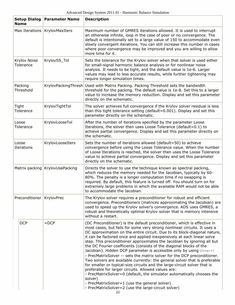
Advanced Design System 2011.01 - Harmonic Balance Simulation
33
Setup DialogName
Parameter Name Description
Max Iterations KrylovMaxIters Maximum number of GMRES iterations allowed. It is used to interruptan otherwise infinite, loop in the case of poor or no convergence. Thedefault is intentionally set to a large value of 150 to accommodate evenslowly convergent iterations. You can still increase this number in caseswhere poor convergence may be improved and you are willing to allowmore time for it.
Krylov NoiseTolerance
KrylovSS_Tol Sets the tolerance for the Krylov solver when that solver is used eitherfor small-signal harmonic balance analysis or for nonlinear noiseanalysis. It needs to be tight, and the default value is 1e-6. Largervalues may lead to less accurate results, while further tightening mayrequire longer simulation times.
PackingThreshold
KrylovPackingThresh Used with Matrix Packing. Packing Threshold sets the bandwidththreshold for the packing. The default value is 1e-8. Set this to a largervalue to increase the memory reduction. Display and set this parameterdirectly on the schematic.
TightTolerance
KrylovTightTol The solver achieves full convergence if the Krylov solver residual is lessthan this tight tolerance setting (default=0.001). Display and set thisparameter directly on the schematic.
LooseTolerance
KrylovLooseTol After the number of iterations specified by the parameter LooseIterations, the solver then uses Loose Tolerance (default=0.1) toachieve partial convergence. Display and set this parameter directly onthe schematic.
LooseIterations
KrylovLooseIters Sets the number of iterations allowed (default=50) to achieveconvergence before using the Loose Tolerance value. When the numberof Loose Iterations is reached, the solver then uses the Loose Tolerancevalue to achieve partial convergence. Display and set this parameterdirectly on the schematic.
Matrix packing KrylovUsePacking Directs the solver to use the technique known as spectral packing,which reduces the memory needed for the Jacobian, typically by 60-80%. The penalty is a longer computation time if no swapping isrequired. By default, this feature is turned off. You should turn on forextremely large problems in which the available RAM would not be ableto accommodate the Jacobian.
Preconditioner KrylovPrec The Krylov solver requires a preconditioner for robust and efficientconvergence. Preconditioners (matrices approximating the Jacobian) areused to speed up the Krylov solver's convergence. ADS uses GMRES, arobust and theoretically optimal Krylov solver that is memory intensivewithout a restart.
DCP =DCP (DC Preconditioner) is the default preconditioner, which is effective inmost cases, but fails for some very strong nonlinear circuits. It uses aDC approximation on the entire circuit. Due to its block-diagonal nature,it can be factored once and applied inexpensively at each linear solvestep. This preconditioner approximates the Jacobian by ignoring all butthe DC Fourier coefficients (consists of the diagonal blocks of theJacobian). Hidden DCP parameter is accessible only by using Other=:- PrecMatrixSolver -- sets the matrix solver for the DCP preconditioner.Two solvers are available currently: the general solver that is preferablefor smaller or typical-size circuits and the large-circuit solver that ispreferable for larger circuits. Allowed values are:- PrecMatrixSolver=0 (default, the simulator automatically chooses thesolver)- PrecMatrixSolver=1 (use the general solver)- PrecMatrixSolver=2 (use the large-circuit solver)
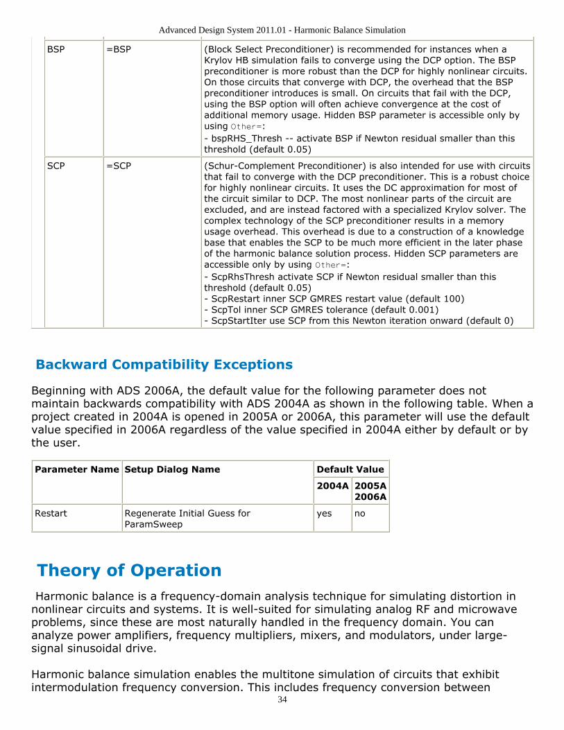
Advanced Design System 2011.01 - Harmonic Balance Simulation
34
BSP =BSP (Block Select Preconditioner) is recommended for instances when aKrylov HB simulation fails to converge using the DCP option. The BSPpreconditioner is more robust than the DCP for highly nonlinear circuits.On those circuits that converge with DCP, the overhead that the BSPpreconditioner introduces is small. On circuits that fail with the DCP,using the BSP option will often achieve convergence at the cost ofadditional memory usage. Hidden BSP parameter is accessible only byusing Other=:- bspRHS_Thresh -- activate BSP if Newton residual smaller than thisthreshold (default 0.05)
SCP =SCP (Schur-Complement Preconditioner) is also intended for use with circuitsthat fail to converge with the DCP preconditioner. This is a robust choicefor highly nonlinear circuits. It uses the DC approximation for most ofthe circuit similar to DCP. The most nonlinear parts of the circuit areexcluded, and are instead factored with a specialized Krylov solver. Thecomplex technology of the SCP preconditioner results in a memoryusage overhead. This overhead is due to a construction of a knowledgebase that enables the SCP to be much more efficient in the later phaseof the harmonic balance solution process. Hidden SCP parameters areaccessible only by using Other=:- ScpRhsThresh activate SCP if Newton residual smaller than thisthreshold (default 0.05)- ScpRestart inner SCP GMRES restart value (default 100)- ScpTol inner SCP GMRES tolerance (default 0.001)- ScpStartIter use SCP from this Newton iteration onward (default 0)
Backward Compatibility Exceptions
Beginning with ADS 2006A, the default value for the following parameter does notmaintain backwards compatibility with ADS 2004A as shown in the following table. When aproject created in 2004A is opened in 2005A or 2006A, this parameter will use the defaultvalue specified in 2006A regardless of the value specified in 2004A either by default or bythe user.
Parameter Name Setup Dialog Name Default Value
2004A 2005A2006A
Restart Regenerate Initial Guess forParamSweep
yes no
Theory of Operation Harmonic balance is a frequency-domain analysis technique for simulating distortion innonlinear circuits and systems. It is well-suited for simulating analog RF and microwaveproblems, since these are most naturally handled in the frequency domain. You cananalyze power amplifiers, frequency multipliers, mixers, and modulators, under large-signal sinusoidal drive.
Harmonic balance simulation enables the multitone simulation of circuits that exhibitintermodulation frequency conversion. This includes frequency conversion between
Advanced Design System 2011.01 - Harmonic Balance Simulation
35
harmonics. Not only can the circuit itself produce harmonics, but each signal source(stimulus) can also produce harmonics or small-signal sidebands. The stimulus can consistof up to twelve nonharmonically related sources. The total number of frequencies in thesystem is limited only by such practical considerations as memory, swap space, andsimulation speed.
The Simulation Process
The harmonic balance method is iterative. It is based on the assumption that for a givensinusoidal excitation there exists a steady-state solution that can be approximated tosatisfactory accuracy by means of a finite Fourier series. Consequently, the circuit nodevoltages take on a set of amplitudes and phases for all frequency components. Thecurrents flowing from nodes into linear elements, including all distributed elements, arecalculated by means of a straightforward frequency-domain linear analysis. Currents fromnodes into nonlinear elements are calculated in the time-domain. Generalized Fourieranalysis is used to transform from the time-domain to the frequency-domain.
The Harmonic Balance solution is approximated by truncated Fourier series and thismethod is inherently incapable of representing transient behavior. The time-derivative canbe computed exactly with boundary conditions, v(0)=v(t), automatically satisfied for alliterates.
The truncated Fourier approximation + N circuit equations results in a residual functionthat is minimized.
N x M nonlinear algebraic equations are solved for the Fourier coefficients using Newton'smethod and the inner linear problem is solved by:
Direct method (Gaussian elimination) for small problems.Krylov-subspace method (e.g. GMRES) for larger problems.
Nonlinear devices (transistors, diodes, etc.) in Harmonic Balance are evaluated (sampled)in the time-domain and converted to frequency-domain via the FFT.
A frequency-domain representation of all currents flowing away from all nodes isavailable. According to Kirchoff's Current Law (KCL), these currents should sum to zero atall nodes. The probability of obtaining this result on the first iteration is extremely small.
Therefore, an error function is formulated by calculating the sum of currents at all nodes.This error function is a measure of the amount by which KCL is violated and is used toadjust the voltage amplitudes and phases. If the method converges (that is, if the errorfunction is driven to a given small value), then the resulting voltage amplitudes andphases approximate the steady-state solution. The following flow chart presents a visualrepresentation of the process:
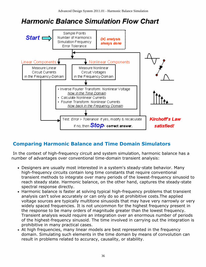
Advanced Design System 2011.01 - Harmonic Balance Simulation
36
Comparing Harmonic Balance and Time Domain Simulators
In the context of high-frequency circuit and system simulation, harmonic balance has anumber of advantages over conventional time-domain transient analysis:
Designers are usually most interested in a system's steady-state behavior. Manyhigh-frequency circuits contain long time constants that require conventionaltransient methods to integrate over many periods of the lowest-frequency sinusoid toreach steady state. Harmonic balance, on the other hand, captures the steady-statespectral response directly.Harmonic balance is faster at solving typical high-frequency problems that transientanalysis can't solve accurately or can only do so at prohibitive costs.The appliedvoltage sources are typically multitone sinusoids that may have very narrowly or verywidely spaced frequencies. It is not uncommon for the highest frequency present inthe response to be many orders of magnitude greater than the lowest frequency.Transient analysis would require an integration over an enormous number of periodsof the highest-frequency sinusoid. The time involved in carrying out the integration isprohibitive in many practical cases.At high frequencies, many linear models are best represented in the frequencydomain. Simulating such elements in the time domain by means of convolution canresult in problems related to accuracy, causality, or stability.
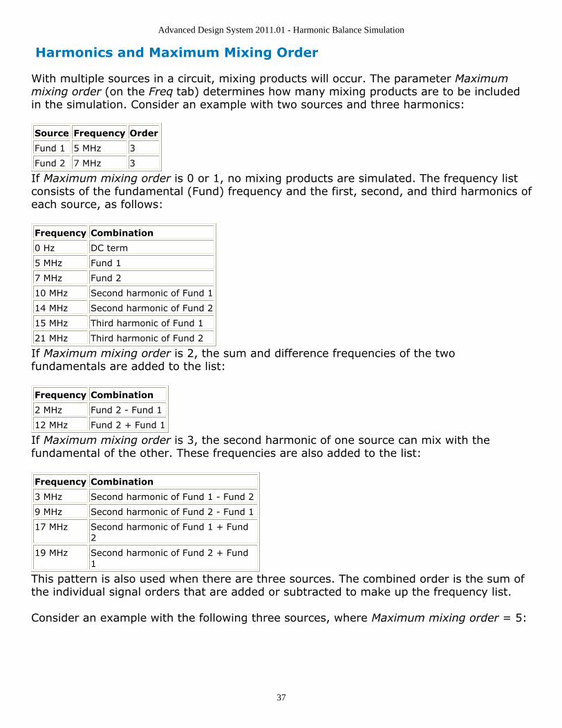
Advanced Design System 2011.01 - Harmonic Balance Simulation
37
Harmonics and Maximum Mixing Order
With multiple sources in a circuit, mixing products will occur. The parameter Maximummixing order (on the Freq tab) determines how many mixing products are to be includedin the simulation. Consider an example with two sources and three harmonics:
Source Frequency Order
Fund 1 5 MHz 3
Fund 2 7 MHz 3
If Maximum mixing order is 0 or 1, no mixing products are simulated. The frequency listconsists of the fundamental (Fund) frequency and the first, second, and third harmonics ofeach source, as follows:
Frequency Combination
0 Hz DC term
5 MHz Fund 1
7 MHz Fund 2
10 MHz Second harmonic of Fund 1
14 MHz Second harmonic of Fund 2
15 MHz Third harmonic of Fund 1
21 MHz Third harmonic of Fund 2
If Maximum mixing order is 2, the sum and difference frequencies of the twofundamentals are added to the list:
Frequency Combination
2 MHz Fund 2 - Fund 1
12 MHz Fund 2 + Fund 1
If Maximum mixing order is 3, the second harmonic of one source can mix with thefundamental of the other. These frequencies are also added to the list:
Frequency Combination
3 MHz Second harmonic of Fund 1 - Fund 2
9 MHz Second harmonic of Fund 2 - Fund 1
17 MHz Second harmonic of Fund 1 + Fund2
19 MHz Second harmonic of Fund 2 + Fund1
This pattern is also used when there are three sources. The combined order is the sum ofthe individual signal orders that are added or subtracted to make up the frequency list.
Consider an example with the following three sources, where Maximum mixing order = 5:
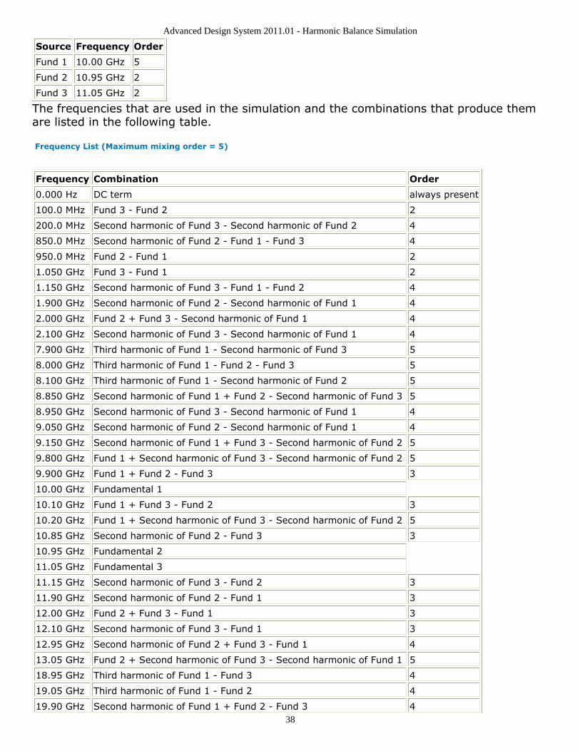
Advanced Design System 2011.01 - Harmonic Balance Simulation
38
Source Frequency Order
Fund 1 10.00 GHz 5
Fund 2 10.95 GHz 2
Fund 3 11.05 GHz 2
The frequencies that are used in the simulation and the combinations that produce themare listed in the following table.
Frequency List (Maximum mixing order = 5)
Frequency Combination Order
0.000 Hz DC term always present
100.0 MHz Fund 3 - Fund 2 2
200.0 MHz Second harmonic of Fund 3 - Second harmonic of Fund 2 4
850.0 MHz Second harmonic of Fund 2 - Fund 1 - Fund 3 4
950.0 MHz Fund 2 - Fund 1 2
1.050 GHz Fund 3 - Fund 1 2
1.150 GHz Second harmonic of Fund 3 - Fund 1 - Fund 2 4
1.900 GHz Second harmonic of Fund 2 - Second harmonic of Fund 1 4
2.000 GHz Fund 2 + Fund 3 - Second harmonic of Fund 1 4
2.100 GHz Second harmonic of Fund 3 - Second harmonic of Fund 1 4
7.900 GHz Third harmonic of Fund 1 - Second harmonic of Fund 3 5
8.000 GHz Third harmonic of Fund 1 - Fund 2 - Fund 3 5
8.100 GHz Third harmonic of Fund 1 - Second harmonic of Fund 2 5
8.850 GHz Second harmonic of Fund 1 + Fund 2 - Second harmonic of Fund 3 5
8.950 GHz Second harmonic of Fund 3 - Second harmonic of Fund 1 4
9.050 GHz Second harmonic of Fund 2 - Second harmonic of Fund 1 4
9.150 GHz Second harmonic of Fund 1 + Fund 3 - Second harmonic of Fund 2 5
9.800 GHz Fund 1 + Second harmonic of Fund 3 - Second harmonic of Fund 2 5
9.900 GHz Fund 1 + Fund 2 - Fund 3 3
10.00 GHz Fundamental 1
10.10 GHz Fund 1 + Fund 3 - Fund 2 3
10.20 GHz Fund 1 + Second harmonic of Fund 3 - Second harmonic of Fund 2 5
10.85 GHz Second harmonic of Fund 2 - Fund 3 3
10.95 GHz Fundamental 2
11.05 GHz Fundamental 3
11.15 GHz Second harmonic of Fund 3 - Fund 2 3
11.90 GHz Second harmonic of Fund 2 - Fund 1 3
12.00 GHz Fund 2 + Fund 3 - Fund 1 3
12.10 GHz Second harmonic of Fund 3 - Fund 1 3
12.95 GHz Second harmonic of Fund 2 + Fund 3 - Fund 1 4
13.05 GHz Fund 2 + Second harmonic of Fund 3 - Second harmonic of Fund 1 5
18.95 GHz Third harmonic of Fund 1 - Fund 3 4
19.05 GHz Third harmonic of Fund 1 - Fund 2 4
19.90 GHz Second harmonic of Fund 1 + Fund 2 - Fund 3 4
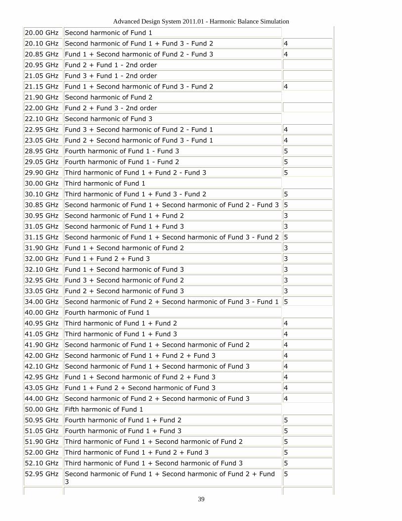
Advanced Design System 2011.01 - Harmonic Balance Simulation
39
20.00 GHz Second harmonic of Fund 1
20.10 GHz Second harmonic of Fund 1 + Fund 3 - Fund 2 4
20.85 GHz Fund 1 + Second harmonic of Fund 2 - Fund 3 4
20.95 GHz Fund 2 + Fund 1 - 2nd order
21.05 GHz Fund 3 + Fund 1 - 2nd order
21.15 GHz Fund 1 + Second harmonic of Fund 3 - Fund 2 4
21.90 GHz Second harmonic of Fund 2
22.00 GHz Fund 2 + Fund 3 - 2nd order
22.10 GHz Second harmonic of Fund 3
22.95 GHz Fund 3 + Second harmonic of Fund 2 - Fund 1 4
23.05 GHz Fund 2 + Second harmonic of Fund 3 - Fund 1 4
28.95 GHz Fourth harmonic of Fund 1 - Fund 3 5
29.05 GHz Fourth harmonic of Fund 1 - Fund 2 5
29.90 GHz Third harmonic of Fund 1 + Fund 2 - Fund 3 5
30.00 GHz Third harmonic of Fund 1
30.10 GHz Third harmonic of Fund 1 + Fund 3 - Fund 2 5
30.85 GHz Second harmonic of Fund 1 + Second harmonic of Fund 2 - Fund 3 5
30.95 GHz Second harmonic of Fund 1 + Fund 2 3
31.05 GHz Second harmonic of Fund 1 + Fund 3 3
31.15 GHz Second harmonic of Fund 1 + Second harmonic of Fund 3 - Fund 2 5
31.90 GHz Fund 1 + Second harmonic of Fund 2 3
32.00 GHz Fund 1 + Fund 2 + Fund 3 3
32.10 GHz Fund 1 + Second harmonic of Fund 3 3
32.95 GHz Fund 3 + Second harmonic of Fund 2 3
33.05 GHz Fund 2 + Second harmonic of Fund 3 3
34.00 GHz Second harmonic of Fund 2 + Second harmonic of Fund 3 - Fund 1 5
40.00 GHz Fourth harmonic of Fund 1
40.95 GHz Third harmonic of Fund 1 + Fund 2 4
41.05 GHz Third harmonic of Fund 1 + Fund 3 4
41.90 GHz Second harmonic of Fund 1 + Second harmonic of Fund 2 4
42.00 GHz Second harmonic of Fund 1 + Fund 2 + Fund 3 4
42.10 GHz Second harmonic of Fund 1 + Second harmonic of Fund 3 4
42.95 GHz Fund 1 + Second harmonic of Fund 2 + Fund 3 4
43.05 GHz Fund 1 + Fund 2 + Second harmonic of Fund 3 4
44.00 GHz Second harmonic of Fund 2 + Second harmonic of Fund 3 4
50.00 GHz Fifth harmonic of Fund 1
50.95 GHz Fourth harmonic of Fund 1 + Fund 2 5
51.05 GHz Fourth harmonic of Fund 1 + Fund 3 5
51.90 GHz Third harmonic of Fund 1 + Second harmonic of Fund 2 5
52.00 GHz Third harmonic of Fund 1 + Fund 2 + Fund 3 5
52.10 GHz Third harmonic of Fund 1 + Second harmonic of Fund 3 5
52.95 GHz Second harmonic of Fund 1 + Second harmonic of Fund 2 + Fund3
5
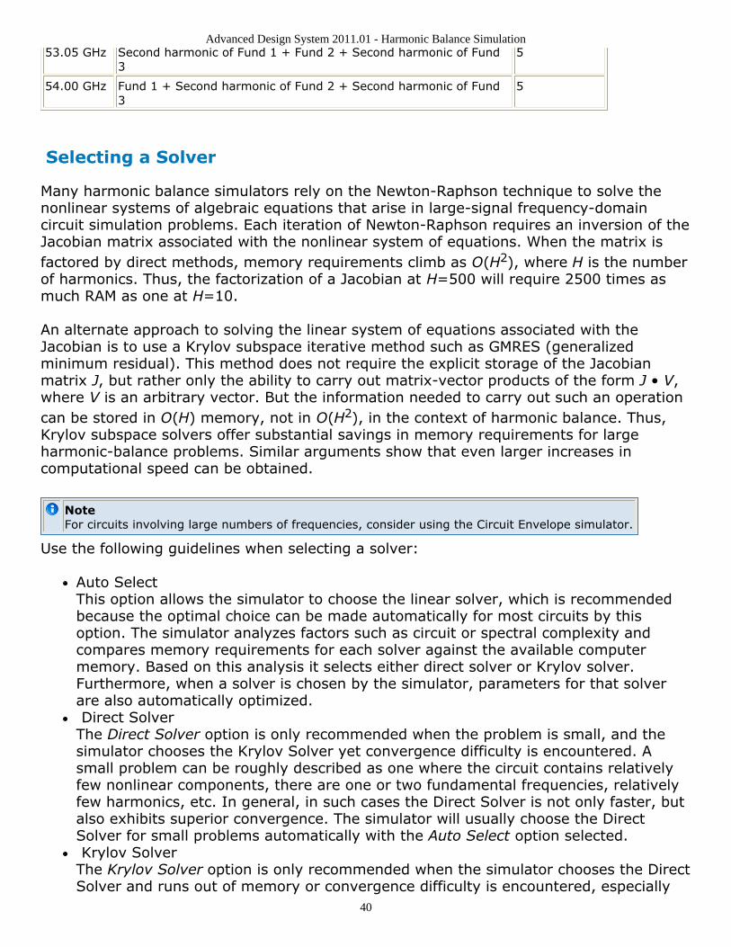
Advanced Design System 2011.01 - Harmonic Balance Simulation
40
53.05 GHz Second harmonic of Fund 1 + Fund 2 + Second harmonic of Fund3
5
54.00 GHz Fund 1 + Second harmonic of Fund 2 + Second harmonic of Fund3
5
Selecting a Solver
Many harmonic balance simulators rely on the Newton-Raphson technique to solve thenonlinear systems of algebraic equations that arise in large-signal frequency-domaincircuit simulation problems. Each iteration of Newton-Raphson requires an inversion of theJacobian matrix associated with the nonlinear system of equations. When the matrix isfactored by direct methods, memory requirements climb as O(H2), where H is the numberof harmonics. Thus, the factorization of a Jacobian at H=500 will require 2500 times asmuch RAM as one at H=10.
An alternate approach to solving the linear system of equations associated with theJacobian is to use a Krylov subspace iterative method such as GMRES (generalizedminimum residual). This method does not require the explicit storage of the Jacobianmatrix J, but rather only the ability to carry out matrix-vector products of the form J • V,where V is an arbitrary vector. But the information needed to carry out such an operationcan be stored in O(H) memory, not in O(H2), in the context of harmonic balance. Thus,Krylov subspace solvers offer substantial savings in memory requirements for largeharmonic-balance problems. Similar arguments show that even larger increases incomputational speed can be obtained.
NoteFor circuits involving large numbers of frequencies, consider using the Circuit Envelope simulator.
Use the following guidelines when selecting a solver:
Auto SelectThis option allows the simulator to choose the linear solver, which is recommendedbecause the optimal choice can be made automatically for most circuits by thisoption. The simulator analyzes factors such as circuit or spectral complexity andcompares memory requirements for each solver against the available computermemory. Based on this analysis it selects either direct solver or Krylov solver.Furthermore, when a solver is chosen by the simulator, parameters for that solverare also automatically optimized. Direct SolverThe Direct Solver option is only recommended when the problem is small, and thesimulator chooses the Krylov Solver yet convergence difficulty is encountered. Asmall problem can be roughly described as one where the circuit contains relativelyfew nonlinear components, there are one or two fundamental frequencies, relativelyfew harmonics, etc. In general, in such cases the Direct Solver is not only faster, butalso exhibits superior convergence. The simulator will usually choose the DirectSolver for small problems automatically with the Auto Select option selected. Krylov SolverThe Krylov Solver option is only recommended when the simulator chooses the DirectSolver and runs out of memory or convergence difficulty is encountered, especially
Advanced Design System 2011.01 - Harmonic Balance Simulation
41
when solving large problems. A large problem can roughly be described as one wherememory usage exceeds 400 MB or the memory capacity of the computer (whicheveroccurs first). A problem may be large because of a large number of nonlinearcomponents, a large number of harmonics required for simulation, or both. Thesimulator will usually choose the Krylov Solver for large problems automatically withthe Auto Select option selected. Krylov is less robust than the Direct Solver methodbecause it uses iterative algorithms to solve the matrix equations. However, it ismuch faster and requires much less memory than the Direct Solver for largeproblems.
In most cases, Auto Select will choose the most effective solver automatically. ChooseDirect Solver or Krylov Solver only when the Auto Select option cannot deliver satisfactoryperformance for a certain circuit.
Simulation time may not be a good indicator for the choice. Some problems are small, butstill take a long time to simulate because parameters are being swept over many steps;such a problem should really be viewed as a sequence of small problems, and thus Krylovis not necessarily applicable. When a parameter is swept, if it takes X seconds to computea single solution using the Krylov solver, it will probably take approximately 10X secondsto compute 10 solutions. On the other hand, if it takes Y seconds to compute a singlesolution using the direct solver, it will probably take far less than 10Y seconds to compute10 swept steps of the analysis.
For system-level applications (behavioral mixers, amplifiers, etc.), the Krylov solvershould be the preferred method of solution, as it is very robust in this area. For sometransistor-level circuits, the Krylov solver may experience convergence difficulties at highinput power levels. If this occurs, an analysis using the direct solver or the Envelopesimulator should be attempted.
To select a specific solver:
Select the Solver tab in the Harmonic Balance setup dialog box.1.Select the desired solver option. In general, we recommend that you accept the2.defaults and click OK to close the dialog box (or select another tab to set additionalsimulation specifications, as needed).
For descriptions of the options and parameters associated with the solvers, click Helpfrom the dialog box.
Reusing Simulation Solutions
Harmonic balance simulation solutions can be saved and used later as an initial guess foranother simulation, including harmonic balance, large-signal S-parameter, gaincompression, or circuit envelope. Reusing solutions can save a considerable amount ofsimulation time. For example, you can save a harmonic balance solution and perform anonlinear noise simulation, using this saved solution as the initial guess. Doing so removesthe time required to re-compute the nonlinear HB solution. Another instance would be tosolve for an initial harmonic balance solution and then sweep a parameter to see the
Advanced Design System 2011.01 - Harmonic Balance Simulation
42
changes.
To save a simulation for reuse:
Add the desired simulation component to your schematic-harmonic balance, large-1.signal S-parameter, gain compression, or envelope. Double-click to edit it.Select the Params tab. If using the Envelope controller, select the HB Params tab.2.Enable Write Final Solution. Enter a filename and any extension, or use the default3.which is <workspace_name>.hbs. The file will be saved in the networks folder of theworkspace.Click OK. When you run the next simulation, the solution will be saved.4.
To select a solution file to be used as the initial guess:
Place the simulation component of interest on the schematic if one is not present,1.then double-click to edit it.Select the Params tab.2.Enable Use Initial Guess. Enter the filename and extension.3.To view any messages regarding how the initial guess affects the simulation, add an4.Options component and set the Annotate parameter. For more information on how todo this, refer to the topic Reusing Simulation Solutions (cktsim).
NoteSince harmonic balance simulations also use the DC solution, for optimum speed improvement, boththe DC solution and the HB solution should be saved and re-used as initial guesses.
The initial guess file does not need to contain all of the harmonic balance frequencies.For example, you could perform a one-tone simulation with a very nonlinear LO, savethe solution, and then use it as an initial guess in a two-tone simulation.
The exact frequencies do not have to match between the present analysis and the initialguess solution. However, the fundamental indexes should match. For example, a solutionsaved from a two-tone analysis with Freq[1] = 1GHz and Freq[2] = 1kHz would not be agood match for a simulation with Freq[1] = 1kHz and Freq[2] = 1 GHz.
Troubleshooting a SimulationThis section presents suggestions to help achieve a successful simulation that is fast andaccurate. It includes the following topics:
Selecting the Number of Harmonics describes how to select an optimum number ofharmonics in a simulation to ensure accuracy and minimize simulation time.Reducing Simulation Time describes other methods to help reduce simulation time.Solving Convergence Problems offers a variety of methods to try if your simulation isfailing because it cannot converge.Oversampling to Prevent Aliasing describes how the Oversampling parameter can beset to prevent aliasing during a simulation.Linearizing Nonlinear Devices describes how making a circuit more linear can improvethe chances of a successful simulation.
Advanced Design System 2011.01 - Harmonic Balance Simulation
43
Also, refer to the troubleshooting sections in DC Simulation (cktsimdc) and AC Simulation(cktsimac).
Selecting the Number of Harmonics
The number of harmonics needed to simulate a circuit accurately depends onnonlinearities in the circuit, the accuracy desired, and the acceptable simulation time.
Consider the following in choosing or changing the number of harmonics:
If the simulation has been run with fewer than the minimum number of harmonicsthat are required for convergence, no solution is found. The simulation may notconverge.If the simulation has been run with the minimum number of harmonics that arerequired for convergence, the simulation converges but the results are inaccurate.If the simulation has been run with the optimum number of harmonics that arerequired for convergence, the simulation converges and the results are accurate.If the simulation has been run with the more than the optimum number of harmonicsthat are required for convergence, the simulation converges and the results areaccurate, but the simulation takes longer than necessary.
To verify that the simulation is accurate, choose a certain number of harmonics andperform the simulation. Then double the number of harmonics and simulate the circuitagain.
If the results are the same, the first choice used enough harmonics for an accuratesimulation. If the results differ, double the second choice and run the simulation again.Continue this procedure until there is no change (or there is an acceptable change) in thesimulation after the number of harmonics is doubled.
Reducing Simulation Time
To reduce simulation time while still maintaining an accurate simulation, consider thefollowing factors in your simulation and make the appropriate trade-offs:
Simulation frequencies - The number of harmonically unrelated frequenciesapplied to a network increases the required memory and simulation timeconsiderably.Power levels - Power levels that increase the degree of nonlinearity will increasesimulation time.Harmonics - The more harmonics to be considered, the greater the memory andsimulation time required.Sample points - Increasing the amount of oversampling may result in a modestincrease in simulation time, unless the Krylov option is selected. (Refer toOversampling to Prevent Aliasing).
Advanced Design System 2011.01 - Harmonic Balance Simulation
44
Error tolerances - The smaller the error tolerances, the greater the simulation time.Device models - The number of nonlinear elements in a device model and thenumber of devices used in the circuit will affect both the memory and simulation timerequired.
Solving Convergence Problems
Nonconvergence is a numerical problem encountered by the harmonic balance simulatorwhen it cannot reach a solution, within a given tolerance, after a given number ofnumerical iterations. There is no one specific solution for solving convergence problems.However, consider the following guidelines:
Increase the value of Order (or other harmonic controls); this is the most basictechnique for solving convergence problems. However, if the time penalty for doingso becomes severe, other methods should be attempted.Use the Status server window as the main tool in solving convergence problems (setStatusLevel=4). For each Newton iteration the L-1 norm of the residuals throughoutthe circuit is printed: a "*" indicates a full Newton step (vs. a Samanskii step).Convergence criteria are controlled by Voltage relative tolerance, and Current relativetolerance. In general, convergence speed is improved by increasing these values, butat the expense of accuracy. Similarly, the smaller these values are, the moreaccurate the results but the slower the convergence. To set these values, use theConvergence tab on the Options component.Newton convergence issues with Krylov methods (because linear problem solutionscan only approximate) can be improved by using better preconditioners.For non-convergence due to tight tolerances, monitor the residuals in the StatusServer window:
Increase I_AbsTol if the circuit is converging to within a few pA but not quite toI_AbsTol=1pA.Increase I_RelTol if the problem is with nodes associated with large currents.Increase I_AbsTol if the small current nodes are the issue.Relax voltage tolerances for failure in the Newton update criterion.
Set the Oversample parameter to a value greater than 1.0, such as 2.0 or 4.0.However, remember that although this can often solve convergence problems, it doesso at the cost of computer memory and simulation time. For multiple-tone harmonicbalance simulations, make sure that the largest signal in the circuit is assigned toFreq[1]. The simulator's FFT algorithm is set up so that aliasing errors are much lesslikely to affect Freq[1] than any other tone. For instance, assign the LO signal in areceiver chain to Freq[1] and the RF signal Freq[2]. For more information, refer toOversampling to Prevent Aliasing.Circuits that contain MOSFETS may fail to converge as a result of inherent limitationsin the SPICE MOSFET model (Level 1, 2 and 3). This problem can often becircumvented by using the device's Xqc parameter . Setting Xqc to a nonzero valueallows the simulator to use a charge-based model (based upon the work of Ward andDutton) for the gate capacitance. This often enables the simulator to converge, but atthe cost of extracting an extra SPICE model parameter. Also, time-domainsimulations usually handle MOSFETs with no difficulty.
Advanced Design System 2011.01 - Harmonic Balance Simulation
45
NoteThere are many references in the literature to SPICE MOSFET models. One is Antognetti andMossobrio, Semiconductor Device Modeling with SPICE, Second Edition, McGraw-Hill, 1993.
Harmonic balance simulation uses the parameters Current relative tolerance, Voltagerelative tolerance, Current absolute tolerance, and Voltage absolute tolerance in thesame way as DC simulation does. For more information, see Setting ConvergenceOptions (cktsim). Do not use more harmonics than you really need. Too many harmonics canintroduce so many unknowns to the solution that the simulator cannot find an answer(because the Jacobian becomes ill-conditioned). Removing harmonics can make thecircuit easier (and faster) to solve, but if too many harmonics are removed, Fourierseries truncation errors will become important. The simulator will converge on ananswer, but it will not be accurate. Refer to Selecting the Number of Harmonics forinstructions on how to minimize the number of harmonics.If the simulator cannot find a solution, it will attempt to do source stepping. This setsall large-signal AC sources to zero (leaving DC sources alone) and attempts toachieve convergence at a lower level. Starting from this solution point, the simulatorwill try to converge at the original level by repeatedly solving the circuit atincrementally increasing source levels, using the results of each simulation as theinitial guess for the next. Very rarely, circuits can exhibit a bizarre behavior that cancause this technique to fail.If the harmonic balance simulation cannot converge on a solution within a givennumber of iterations, try increasing the limit in the Max. Iterations field, under theParams tab.The internal circuit simulator engine in ADS (ADSsim) runs from a netlist. ADS writesa netlist file (netlist.log) before invoking ADSsim. The order of the components andmodel definitions in the netlist determine the initial Jacobian matrix ordering. Thismatrix ordering can affect the efficiency of the Jacobian factorization and cause eithera simulation slow down or non-convergence.For convergence problems due to errors in the component model equations (incorrectderivatives, etc.) make sure ancient Berkeley MOSFET Level 1, 2, 3 are not theculprit and that the latest model version is used (especially BSIM3 models). Modelproblems can cause the Newton residual to hit a threshold (greater than theconvergence criteria tolerances) and stale the convergence process or even exhibitrandom jumps (sudden increase in value). Set the device's Xqc parameter to anonzero value to allow the simulator to use a charge-based model for the gatecapacitance. This often enables convergence, but at the cost of extracting an extraSPICE model parameter.
Sweeps as Convergence Tools
Continuation methods provide a sequence of initial guesses that are sufficiently close tothe solution to assure Newton's method convergence in Harmonic Balance. Sweeps can beused to formulate a specialized continuation method geared towards the particular circuitproblem.
Try sweeping a parameter to correct a convergence problem. Find a circuit element that,
Advanced Design System 2011.01 - Harmonic Balance Simulation
46
when set to some different value, makes the circuit more linear. For instance, in anamplifier circuit there may be a resistor that can be used to lower the amplifier's gain. Thesimulator may be able to find a solution to the circuit under a low-gain condition. Then, ifthe component's value is swept toward the desired value, the simulator may be able tofind a final solution. Start with a value that works, and stop with the desired value. Also,select Restart, on the Initial Guess tab. Usually, a better initial guess at each step helpsthe simulator to converge.
The two main ways to perform sweeps are:
HB sweep within the HB controller. This is preferred for most sweeps, exceptfrequency.Parameter sweep using a separate sweep controller.
Convergence and the Samanskii Steps
The Samanskii constant is a real non-negative number that is used to determine whetherthe simulator can skip the Jacobian evaluation in some iterations, and just reuse anapproximate Jacobian instead (Samanskii steps). The Samanskii steps can significantlyspeed up the solution process. However, using an approximate Jacobian, particularly for alarger number of iterations, may result in poor or even no convergence. The constant isused in two ways. First, it becomes a more absolute measure when it is smaller. It thenapproaches the requirement that each iteration reduces the relevant norm by one-third.
Decreasing the Samanskii constant beyond a certain point (which in turn depends on thequality of the most recent Newton step) will make no difference. However, setting theSamanskii constant to zero will effectively disable any Samanskii steps altogether.
Increasing the Samanskii constant relaxes this requirements in general, but the conditionbecomes more dependent on the quality of the standard most recent Newton iteration. Inother words, a more rapid convergence of the Newton step would also require betterconvergence of the Samanskii steps.
The default Samanskii constant of 2.0 corresponds to the quality of the Newton step suchthat the norm is reduced by 50% (decreasing the Samanskii constant will not make anydifference if this is the case). Such a cut-off value gets larger with a more significant normreduction of the Newton step. For example, an 83% norm reduction would result in a cut-off value of 10.
NoteTo edit this parameter, select the Display tab in the Harmonic Balance Simulation component and setSamanskiiConstant to display on the schematic page. You can then edit the parameter directly on theschematic.
Convergence and Arc-Length Continuation
Arc-length continuation is an extremely robust algorithm. If it fails, try all other

Advanced Design System 2011.01 - Harmonic Balance Simulation
47
convergence remedies first before adjusting arc-length parameters:
MaxStepRatio controls the maximum number of continuation steps (default 100).MaxShrinkage controls the minimum size of the arc-length step (default 1e-5).ArcMaxStep limits the maximum size of the arc-length step (default is 0, i.e. nolimiting).ArcMinValue & ArcMaxValue define the allowed range for the variation of thecontinuation parameter.
Oversampling to Prevent Aliasing
Oversampling increases the accuracy of the solution by reducing the FFT aliasing error,and improves convergence for circuits with many nonlinear devices.
Aliasing error is introduced during the evaluation of nonlinear devices when a timewaveform is converted into a spectrum. Aliasing is caused by using too few time-points torepresent the time waveform. The Nyquist criterion states that to avoid aliasing errors, thesampling frequency should be at least twice the highest frequency present in the timewaveform. If not, error is introduced into the high-frequency Fourier coefficients. The onlyway to eliminate aliasing error is to increase the sampling rate (that is, to increase thenumber of data points). This can be done by oversampling the time waveform (selectFundamental Oversample, on the Params tab). The relationship between Order,Fundamental Oversample, and the number of samples for a single tone simulation is givenby:
Number of Samples = 2*(Order[1] +1)*Oversample, rounded up to the nearest power oftwo.
For the same value of Order, different values of Fundamental Oversample can yield thesame number of samples. Also, oversampling can occur even with a FundamentalOversample value of 1, because the system rounds the FFT size up to the next power oftwo. This can be seen from the following two tables:
Order Fundamental Oversample Number of Samples
7 1 16
7 2 32
7 3 32
7 4 64
7 5 128
7 6 128
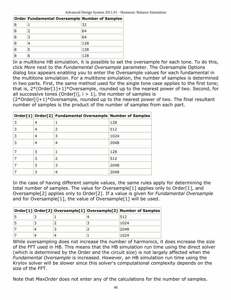
Advanced Design System 2011.01 - Harmonic Balance Simulation
48
Order Fundamental Oversample Number of Samples
8 1 32
8 2 64
8 3 64
8 4 128
8 5 128
8 6 128
In a multitone HB simulation, it is possible to set the oversample for each tone. To do this,click More next to the Fundamental Oversample parameter. The Oversample Optionsdialog box appears enabling you to enter the Oversample values for each fundamental inthe multitone simulation. For a multitone simulation, the number of samples is determinedin two parts. First, the same method used for the single tone case applies to the first tone;that is, 2*(Order[1]+1)*Oversample, rounded up to the nearest power of two. Second, forall successive tones (Order[i], i > 1), the number of samples is(2*Order[i]+1)*Oversample, rounded up to the nearest power of two. The final resultantnumber of samples is the product of the number of samples from each part.
Order[1] Order[2] Fundamental Oversample Number of Samples
3 4 1 128
3 4 2 512
3 4 3 1024
3 4 4 2048
7 3 1 128
7 3 2 512
7 3 3 2048
7 3 4 2048
In the case of having different sample values, the same rules apply for determining thetotal number of samples. The value for Oversample[1] applies only to Order[1], andOversample[2] applies only to Order[2]. If a value is given for Fundamental Oversampleand for Oversample[1], the value of Oversample[1] will be used.
Order[1] Order[2] Oversample[1] Oversample[2] Number of Samples
5 3 1 4 512
5 3 2 3 1024
7 4 3 2 2048
7 4 4 1 1024
While oversampling does not increase the number of harmonics, it does increase the sizeof the FFT used in HB. This means that the HB simulation run time using the direct solver(which is determined by the Order and the circuit size) is not largely affected when theFundamental Oversample is increased. However, an HB simulation run time using theKrylov solver will be slower since this solver's computational complexity depends on thesize of the FFT.
Note that MaxOrder does not enter any of the calculations for the number of samples.
Advanced Design System 2011.01 - Harmonic Balance Simulation
49
Linearizing Nonlinear Devices
The number of nonlinear devices in a network has a dramatic effect on the speed ofharmonic balance simulation. For circuits with a large number of nonlinear devices, suchas those found in RFICs and high-speed digital applications, a standard harmonic balancesimulation may become extremely slow, especially for a multitone simulation or wherelarge numbers of harmonics are involved. However, usually only a few devices in suchcircuits are driven into nonlinearity. Depending upon the application, many devices in thecircuit may be operating in their linear region.
A significant increase in the speed of a harmonic balance simulation can be achievedwithout loss of accuracy if the devices that are operating in the linear region can beidentified and linearized about their DC operating point. When these devices aresimulated, they are treated as other linear elements and are evaluated in the frequencydomain instead of the time domain. The increase in simulation speed is generallyproportional to the number of valid device linearizations.
Advanced Design System 2011.01 - Harmonic Balance Simulation
50
Harmonic Balance for Nonlinear NoiseSimulation The nonlinear noise options in the Harmonic Balance simulator enable you to calculate:
Nonlinear spot noiseSwept noiseNoisy 2-port parameters
There are two methods of noise simulation. One is to use the parameters on the Noise tabin the harmonic balance dialog box. A second method is to use the NoiseCon component.Using NoiseCon components, you can set up several noise simulations, thereby eliminatingthe need to change the values on the Noise tabs in the Harmonic Balance dialog box. WithNoiseCons, you can also set parameters to calculate phase noise.
If you are not familiar with the harmonic balance simulator, refer to Harmonic BalanceBasics (cktsimhb), before continuing with this topic.
Refer to the following topics for details on harmonic balance for nonlinear noisesimulation:
Performing a Nonlinear Noise Simulation describes the minimum setup for calculatingnoise.Performing a Noise Simulation with NoiseCons describes how to set up NoiseCons andinclude them in the simulation.Nonlinear Noise Simulation Description is an overview on how nonlinear noise iscalculated in a simulation.NoiseCon Component Description provides more details about the NoiseConcomponent.NoiseCon Component provides details on the tabs and fields for the Noisecomponent.Harmonic Balance for Oscillator Simulation (cktsimhb), includes information onsetting up noise simulations for oscillators.Harmonic Balance for Mixers (cktsimhb), includes information on setting up noisesimulations for mixers.
Performing a Nonlinear Noise SimulationUse this type of nonlinear noise simulation for spectral noise simulations of circuits that donot employ mixers, such as amplifiers.
For a successful analysis:
Terminate all inputs and outputs with sources or terms. Use sources such as theP_1Tone component in the Sources-Freq Domain palette. Terminate outputs with theTerm component, which can be found on several simulation palettes, including HB.
Advanced Design System 2011.01 - Harmonic Balance Simulation
51
Noise parameters are meaningful only with respect to two ports.Place a noise source where noise is to be injected and edit the component asrequired. Noise sources are found under the Sources-Noise palette.
NoteThe built-in BJT model (BJT_Model) has 1/ f noise sources that can be turned on by setting certainmodel parameters.
NoteWhen simulating noise figure, noise sources should not be added at the input. Noise sources can beadded elsewhere in the circuit, as desired.
From the Simulation-HB palette , select and place the HarmonicBalance component,and double-click to edit it. Select the Noise tab and enable the Nonlinear noisecheckbox.Click the Noise(1) button:
To calculate spot noise, set the Sweep Type to Single point and enter afrequency. If an input frequency is not specified, it is assumed to be the sameas the spot noise frequency. This way, the input and output frequencies are thesame.For a swept noise analysis, set Sweep Type to Linear or Log and define thesweep with Start/Stop or Center/Span values.In the Input frequency field, enter a frequency for the sideband that will mix tothe spot-noise frequency of interest.In the Noise input port field, enter the number of the port at which noise isinjected.In the Noise output port field, enter the number of the Term component atwhich noise is retrieved.
Click the Noise (2) button:To specify the nodes at which noise will be computed, select a node name fromthe Edit list and click Add.The Noise contributors fields enable you to specify and sort the items thatcontribute noise to the simulation, and specify a threshold that determineswhether contributors are reported or not.You can calculate noisy 2-port parameters such as minimum noise figure,optimum source match, and effective noise resistance. These results will appearin the dataset as NFmin, Sopt, and Rn, respectively.For more information about each field, click Help from the HarmonicBalancedialog box.
NoteOnce you have entered these settings, you can switch the noise simulation off by disablingNonlinear noise at the bottom of the dialog. Your settings will remain in the Noise tab andbecome active when Nonlinear noise is enabled again.
Add an Options component to the schematic and set the temperature either byediting Temp=16.85 in the Schematic window, or by selecting the Misc tab andediting Simulation temperature to that value. This temperature, 16.85°C or 290Kelvin, is the standard temperature for noise figure measurement as defined by theIEEE definition for noise figuration.
For more information about nonlinear noise analysis, refer to Nonlinear Noise SimulationDescription.
Advanced Design System 2011.01 - Harmonic Balance Simulation
52
Performing a Noise Simulation with NoiseCons This section describes using the NoiseCon component to enable a noise simulation.
Select NoiseCon from the Simulation-HB palette and place it in the Schematic1.window. Edit it to select the Freq tab and enter noise frequency information.Select the Nodes tab and enter information about the circuit nodes at which to2.compute noise.Select the Misc tab and enter information for noise figure, noise contribution reports3.and noise bandwidth.Select the PhaseNoise tab and enter information about phase noise simulation. Click4.OK.Edit the Harmonic Balance simulation control item to select the NoiseCons tab and5.add the newly placed NoiseCon component to the list of NoiseCons to be simulated.It is not necessary to enable the Nonlinear Noise option at the bottom of the dialogbox.Click OK.
When the simulation is performed, the noise simulation requested in the NoiseCon itemwill be simulated as well.
For more information about NoiseCons, refer to NoiseCon Component Description.
Nonlinear Noise Simulation DescriptionThe results of the harmonic balance simulation are output to the dataset and are thenused to determine the periodic operating point for the nonlinear noise simulation. Theperiodic operating point is the steady-state voltages and currents within the circuit at thefundamental, harmonic, and all mixing frequencies. Every upper and lower noise sidebandis modeled for each large-signal spectral component; consequently, the number of noisefrequencies simulated is double the harmonic frequencies and the sparse-matrix memoryrequirement is quadrupled (unless the Krylov option is used). The result is that a nonlinearnoise simulation requires four times the memory of a normal harmonic balance simulation.Use low values for the parameter Maximum order (under the Freq tab) to limit thedemands on computer memory.
NoteIn nonlinear noise analyses, we recommend that the Options component be used to establish a globalsimulation temperature of 16.85°C if a noise calculation is to be performed. This can be done by editingTemp=16.85 in the Schematic window, or by selecting the Misc tab and editing Simulation temperature tothat value. This temperature, 16.85°C or 290 Kelvin, is the standard temperature for noise figuremeasurement as defined by the IEEE definition for noise figuration.
If computer memory is insufficient for a noise simulation, eliminate the large-signal toneat the input and replace it with a Term component. Also, reduce the number of tones inthe harmonic balance simulation component by 1. The results of the noise figuresimulation should not change significantly. To view an example of how to simulate a
Advanced Design System 2011.01 - Harmonic Balance Simulation
53
mixer's output noise without a large-signal RF input tone, look atexamples/RFIC/Mixers_wrk/NoiseFloor.
If the noise figure is needed, add pins to the circuit. In addition, because the single-sideband definition of noise figure is used, the correct input sideband frequency must bespecified, by the parameter Input frequency (under the Noise tab). This identifies whichinput frequency will mix to the spot-noise frequency of interest.
If the input frequency is not specified, it is assumed to be the same as the spot-noisefrequency. This way, the input and output frequencies are the same, as is typical ofamplifiers. Input frequency is the frequency at which the signal enters the mixer's RF port.For mixers, Input frequency is typically determined by an equation that involves the localoscillator frequency and the noise frequency. Either the sum of or difference betweenthese values is used, depending on whether upconversion or downconversion is takingplace. If an upper or lower sideband cannot be found that agrees with the specified Inputfrequency, a warning is issued and the nearest sideband is used.
If noisy 2-port parameters such as Sopt, Rn, or NFmin are required, select Calculatenoisy two-port parameters. Noise data will be computed only for those nodes requested.The noise voltages and currents scale with the square root of the noise parameter
Bandwidth. The default bandwidth is 1 Hz, so that the results have units of V/ . Theoption Include port noise tells the simulator to include the contributions of port noise inthe analysis of noise voltages and currents. The option Use small-signal frequencies (onby default) gives more accurate results, but also requires more memory.
NoiseCon Component Description The NoiseCon nonlinear noise controller allows more flexibility in the simulation of noisethan can be specified using the Noise(1) and Noise(2) dialog boxes under the Noise tab.The NoiseCon allows the computation of many noise-related quantities, including noisevoltages and currents, differential noise voltages, noise figure and phase noise around anylarge-signal carrier. Multiple NoiseCons can be placed and simulated in one harmonicbalance simulation.
Everything that can be specified in the Noise(1) and Noise(2) dialog boxes can bespecified in a NoiseCon. If you use NoiseCons to perform the noise simulation in harmonicbalance, then you do not need to use the Noise(1) and Noise(2).
In the dataset, noise results from the Noise(1) dialog box appear in the dataset with aname of the form HB1.HB_NOISE.vout.noise, where HB1 is the instance name of theharmonic balance control item. Noise results from a NoiseCon will appear in the datasetwith a name of the form HB1.NC1.vout.noise, where NC1 is the instance name of theNoiseCon.
NoiseCon Component
Advanced Design System 2011.01 - Harmonic Balance Simulation
54
Following are details on the tabs and data fields for the NoiseCon component, which isavailable from the Simulation - HB library.
Two common tabs for controller components include the following:
Output – Selectively save simulation data to a dataset. For details, refer to the topicSelectively Saving and Controlling Simulation Data (cktsim).Display – Control the visibility of simulation parameters on the Schematic. Fordetails, refer to the topic Displaying Simulation Parameters on the Schematic(cktsim).
Setting Up NoiseCon Frequency
The frequency at which noise should be computed is specified on the Freq tab. If a phasenoise simulation is to be performed, as specified on the PhaseNoise tab, the interpretationof these noise frequencies is different. Instead of computing noise directly at thesefrequencies, they are interpreted as offset frequencies from a large signal carrier which isspecified on the PhaseNoise tab. In the following table, names used in netlists and ADSschematics appear under Parameter Name.
NoiseCon Frequency Options
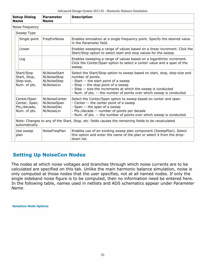
Advanced Design System 2011.01 - Harmonic Balance Simulation
55
Setup DialogName
ParameterName
Description
Noise frequency
Sweep Type
Single point FreqForNoise Enables simulation at a single frequency point. Specify the desired valuein the Parameter field.
Linear Enables sweeping a range of values based on a linear increment. Click theStart/Stop option to select start and stop values for the sweep.
Log Enables sweeping a range of values based on a logarithmic increment.Click the Center/Span option to select a center value and a span of thesweep.
Start/StopStart, Stop,Step-size,Num. of pts.
NLNoiseStartNLNoiseStopNLNoiseStepNLNoiseLin
Select the Start/Stop option to sweep based on start, stop, step-size andnumber of points.- Start -- the start point of a sweep- Stop -- the stop point of a sweep- Step -- size-the increments at which the sweep is conducted- Num. of pts. -- the number of points over which sweep is conducted
Center/SpanCenter, Span,Pts,/decade,Num. of pts.
NLNoiseCenterNLNoiseSpanNLNoiseDecNLNoiseLin
Select the Center/Span option to sweep based on center and span.- Center -- the center point of a sweep- Span -- the span of a sweep- Pts./decade -- number of points per decade- Num. of pts. -- the number of points over which sweep is conducted
Note: Changes to any of the Start, Stop, etc. fields causes the remaining fields to be recalculatedautomatically.
Use sweepplan
NoiseFreqPlan Enables use of an existing sweep plan component (SweepPlan). Selectthis option and enter the name of the plan or select it from the drop-down list.
Setting Up NoiseCon Nodes
The nodes at which noise voltages and branches through which noise currents are to becalculated are specified on this tab. Unlike the main harmonic balance simulation, noise isonly computed at those nodes that the user specifies, not at all named nodes. If only thesingle sideband noise figure is to be computed, then no information need be entered here.In the following table, names used in netlists and ADS schematics appear under ParameterName.
NoiseCon Node Options
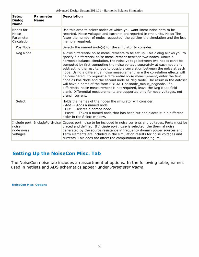
Advanced Design System 2011.01 - Harmonic Balance Simulation
56
SetupDialogName
ParameterName
Description
Nodes forNoiseParameterCalculation
Use this area to select nodes at which you want linear noise data to bereported. Noise voltages and currents are reported in rms units. Note: Thefewer the number of nodes requested, the quicker the simulation and the lessmemory required.
Pos Node Selects the named node(s) for the simulator to consider.
Neg Node Allows differential noise measurements to be set up. This dialog allows you tospecify a differential noise measurement between two nodes. Unlike aharmonic balance simulation, the noise voltage between two nodes can't becomputed by first computing the noise voltage separately at each node andsubtracting the results, due to possible correlation between the noise at eachnode. Using a differential noise measurement here the correlation effects willbe considered. To request a differential noise measurement, enter the firstnode as Pos Node and the second node as Neg Node. The result in the datasetwill have a name of the form HB1.NC1.posnode_minus_negnode. If adifferential noise measurement is not required, leave the Neg Node fieldblank. Differential measurements are supported only for node voltages, notbranch current.
Select Holds the names of the nodes the simulator will consider.- Add -- Adds a named node.- Cut -- Deletes a named node.- Paste -- Takes a named node that has been cut and places it in a differentorder in the Select window.
Include portnoise innode noisevoltages
IncludePortNoise Causes port noise to be included in noise currents and voltages. Ports must beplaced and defined. If Include port noise is selected, the thermal noisegenerated by the source resistance in frequency domain power sources andTerm elements are included in the simulation results for noise voltages andcurrents. This does not affect the computation of noise figure.
Setting Up the NoiseCon Misc. Tab
The NoiseCon noise tab includes an assortment of options. In the following table, namesused in netlists and ADS schematics appear under Parameter Name.
NoiseCon Misc. Options
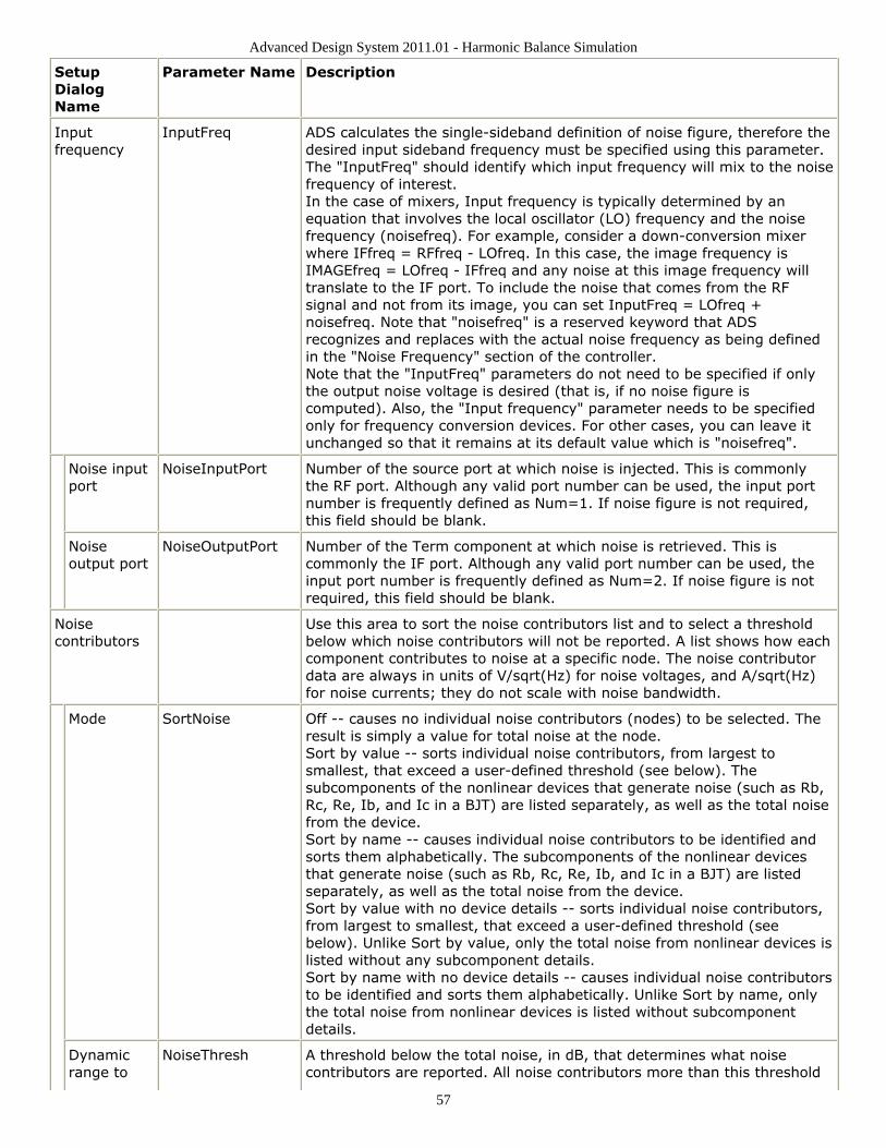
Advanced Design System 2011.01 - Harmonic Balance Simulation
57
SetupDialogName
Parameter Name Description
Inputfrequency
InputFreq ADS calculates the single-sideband definition of noise figure, therefore thedesired input sideband frequency must be specified using this parameter.The "InputFreq" should identify which input frequency will mix to the noisefrequency of interest.In the case of mixers, Input frequency is typically determined by anequation that involves the local oscillator (LO) frequency and the noisefrequency (noisefreq). For example, consider a down-conversion mixerwhere IFfreq = RFfreq - LOfreq. In this case, the image frequency isIMAGEfreq = LOfreq - IFfreq and any noise at this image frequency willtranslate to the IF port. To include the noise that comes from the RFsignal and not from its image, you can set InputFreq = LOfreq +noisefreq. Note that "noisefreq" is a reserved keyword that ADSrecognizes and replaces with the actual noise frequency as being definedin the "Noise Frequency" section of the controller.Note that the "InputFreq" parameters do not need to be specified if onlythe output noise voltage is desired (that is, if no noise figure iscomputed). Also, the "Input frequency" parameter needs to be specifiedonly for frequency conversion devices. For other cases, you can leave itunchanged so that it remains at its default value which is "noisefreq".
Noise inputport
NoiseInputPort Number of the source port at which noise is injected. This is commonlythe RF port. Although any valid port number can be used, the input portnumber is frequently defined as Num=1. If noise figure is not required,this field should be blank.
Noiseoutput port
NoiseOutputPort Number of the Term component at which noise is retrieved. This iscommonly the IF port. Although any valid port number can be used, theinput port number is frequently defined as Num=2. If noise figure is notrequired, this field should be blank.
Noisecontributors
Use this area to sort the noise contributors list and to select a thresholdbelow which noise contributors will not be reported. A list shows how eachcomponent contributes to noise at a specific node. The noise contributordata are always in units of V/sqrt(Hz) for noise voltages, and A/sqrt(Hz)for noise currents; they do not scale with noise bandwidth.
Mode SortNoise Off -- causes no individual noise contributors (nodes) to be selected. Theresult is simply a value for total noise at the node.Sort by value -- sorts individual noise contributors, from largest tosmallest, that exceed a user-defined threshold (see below). Thesubcomponents of the nonlinear devices that generate noise (such as Rb,Rc, Re, Ib, and Ic in a BJT) are listed separately, as well as the total noisefrom the device.Sort by name -- causes individual noise contributors to be identified andsorts them alphabetically. The subcomponents of the nonlinear devicesthat generate noise (such as Rb, Rc, Re, Ib, and Ic in a BJT) are listedseparately, as well as the total noise from the device.Sort by value with no device details -- sorts individual noise contributors,from largest to smallest, that exceed a user-defined threshold (seebelow). Unlike Sort by value, only the total noise from nonlinear devices islisted without any subcomponent details.Sort by name with no device details -- causes individual noise contributorsto be identified and sorts them alphabetically. Unlike Sort by name, onlythe total noise from nonlinear devices is listed without subcomponentdetails.
Dynamicrange to
NoiseThresh A threshold below the total noise, in dB, that determines what noisecontributors are reported. All noise contributors more than this threshold
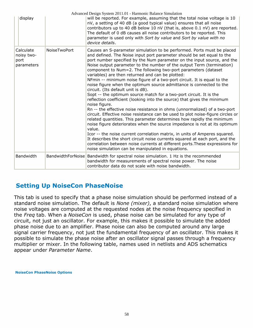
Advanced Design System 2011.01 - Harmonic Balance Simulation
58
display will be reported. For example, assuming that the total noise voltage is 10nV, a setting of 40 dB (a good typical value) ensures that all noisecontributors up to 40 dB below 10 nV (that is, above 0.1 nV) are reported.The default of 0 dB causes all noise contributors to be reported. Thisparameter is used only with Sort by value and Sort by value with nodevice details.
Calculatenoisy two-portparameters
NoiseTwoPort Causes an S-parameter simulation to be performed. Ports must be placedand defined. The Noise input port parameter should be set equal to theport number specified by the Num parameter on the input source, and theNoise output parameter to the number of the output Term (termination)component to Num=2. The following two-port parameters (datasetvariables) are then returned and can be plotted:NFmin -- minimum noise figure of a two-port circuit. It is equal to thenoise figure when the optimum source admittance is connected to thecircuit. (Its default unit is dB).Sopt -- the optimum source match for a two-port circuit. It is thereflection coefficient (looking into the source) that gives the minimumnoise figure.Rn -- the effective noise resistance in ohms (unnormalized) of a two-portcircuit. Effective noise resistance can be used to plot noise-figure circles orrelated quantities. This parameter determines how rapidly the minimumnoise figure deteriorates when the source impedance is not at its optimumvalue.Icor -- the noise current correlation matrix, in units of Amperes squared.It describes the short circuit noise currents squared at each port, and thecorrelation between noise currents at different ports.These expressions fornoise simulation can be manipulated in equations.
Bandwidth BandwidthForNoise Bandwidth for spectral noise simulation. 1 Hz is the recommendedbandwidth for measurements of spectral noise power. The noisecontributor data do not scale with noise bandwidth.
Setting Up NoiseCon PhaseNoise
This tab is used to specify that a phase noise simulation should be performed instead of astandard noise simulation. The default is None (mixer), a standard noise simulation wherenoise voltages are computed at the requested nodes at the noise frequency specified inthe Freq tab. When a NoiseCon is used, phase noise can be simulated for any type ofcircuit, not just an oscillator. For example, this makes it possible to simulate the addedphase noise due to an amplifier. Phase noise can also be computed around any largesignal carrier frequency, not just the fundamental frequency of an oscillator. This makes itpossible to simulate the phase noise after an oscillator signal passes through a frequencymultiplier or mixer. In the following table, names used in netlists and ADS schematicsappear under Parameter Name.
NoiseCon PhaseNoise Options
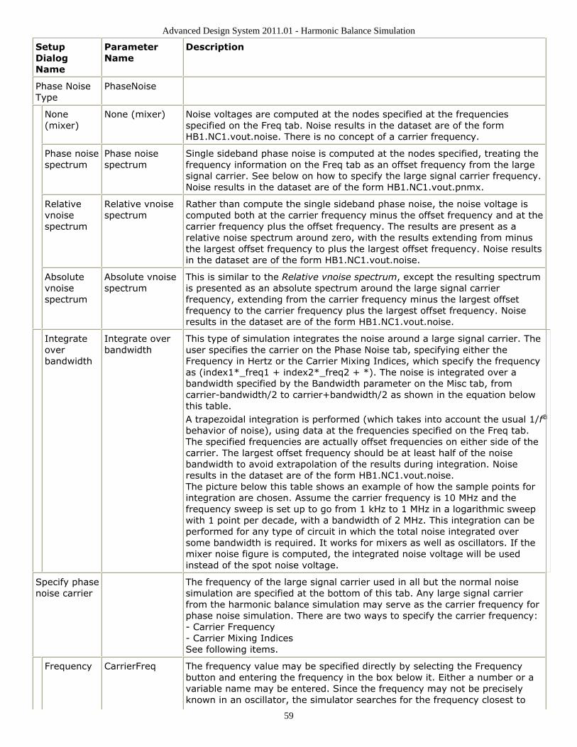
Advanced Design System 2011.01 - Harmonic Balance Simulation
59
SetupDialogName
ParameterName
Description
Phase NoiseType
PhaseNoise
None(mixer)
None (mixer) Noise voltages are computed at the nodes specified at the frequenciesspecified on the Freq tab. Noise results in the dataset are of the formHB1.NC1.vout.noise. There is no concept of a carrier frequency.
Phase noisespectrum
Phase noisespectrum
Single sideband phase noise is computed at the nodes specified, treating thefrequency information on the Freq tab as an offset frequency from the largesignal carrier. See below on how to specify the large signal carrier frequency.Noise results in the dataset are of the form HB1.NC1.vout.pnmx.
Relativevnoisespectrum
Relative vnoisespectrum
Rather than compute the single sideband phase noise, the noise voltage iscomputed both at the carrier frequency minus the offset frequency and at thecarrier frequency plus the offset frequency. The results are present as arelative noise spectrum around zero, with the results extending from minusthe largest offset frequency to plus the largest offset frequency. Noise resultsin the dataset are of the form HB1.NC1.vout.noise.
Absolutevnoisespectrum
Absolute vnoisespectrum
This is similar to the Relative vnoise spectrum, except the resulting spectrumis presented as an absolute spectrum around the large signal carrierfrequency, extending from the carrier frequency minus the largest offsetfrequency to the carrier frequency plus the largest offset frequency. Noiseresults in the dataset are of the form HB1.NC1.vout.noise.
Integrateoverbandwidth
Integrate overbandwidth
This type of simulation integrates the noise around a large signal carrier. Theuser specifies the carrier on the Phase Noise tab, specifying either theFrequency in Hertz or the Carrier Mixing Indices, which specify the frequencyas (index1*_freq1 + index2*_freq2 + *). The noise is integrated over abandwidth specified by the Bandwidth parameter on the Misc tab, fromcarrier-bandwidth/2 to carrier+bandwidth/2 as shown in the equation belowthis table.A trapezoidal integration is performed (which takes into account the usual 1/fa
behavior of noise), using data at the frequencies specified on the Freq tab.The specified frequencies are actually offset frequencies on either side of thecarrier. The largest offset frequency should be at least half of the noisebandwidth to avoid extrapolation of the results during integration. Noiseresults in the dataset are of the form HB1.NC1.vout.noise.The picture below this table shows an example of how the sample points forintegration are chosen. Assume the carrier frequency is 10 MHz and thefrequency sweep is set up to go from 1 kHz to 1 MHz in a logarithmic sweepwith 1 point per decade, with a bandwidth of 2 MHz. This integration can beperformed for any type of circuit in which the total noise integrated oversome bandwidth is required. It works for mixers as well as oscillators. If themixer noise figure is computed, the integrated noise voltage will be usedinstead of the spot noise voltage.
Specify phasenoise carrier
The frequency of the large signal carrier used in all but the normal noisesimulation are specified at the bottom of this tab. Any large signal carrierfrom the harmonic balance simulation may serve as the carrier frequency forphase noise simulation. There are two ways to specify the carrier frequency:- Carrier Frequency- Carrier Mixing IndicesSee following items.
Frequency CarrierFreq The frequency value may be specified directly by selecting the Frequencybutton and entering the frequency in the box below it. Either a number or avariable name may be entered. Since the frequency may not be preciselyknown in an oscillator, the simulator searches for the frequency closest to
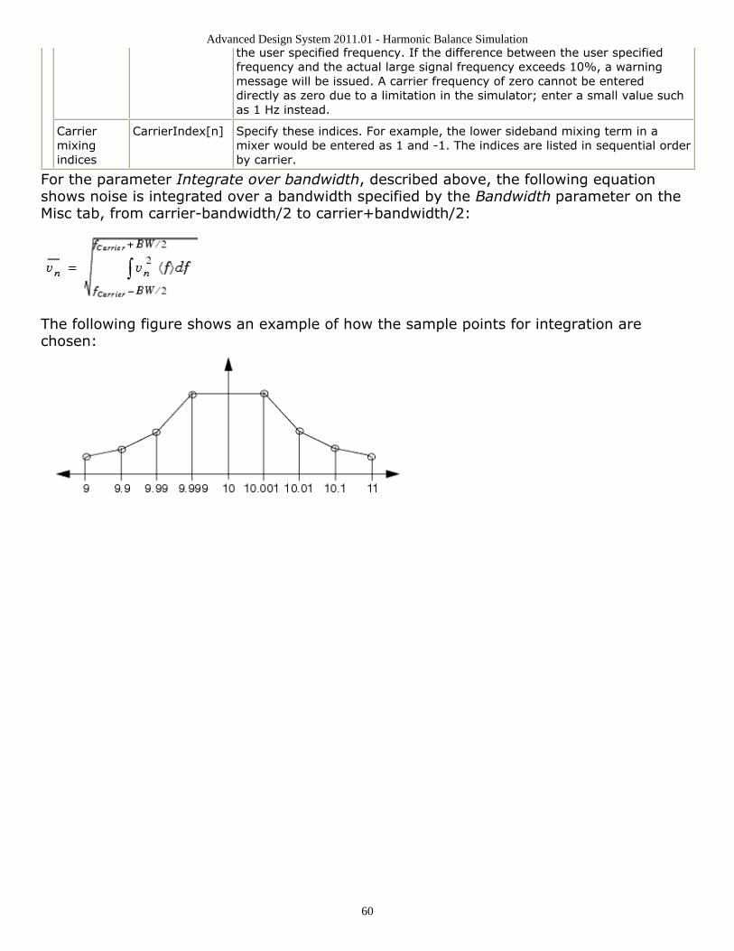
Advanced Design System 2011.01 - Harmonic Balance Simulation
60
the user specified frequency. If the difference between the user specifiedfrequency and the actual large signal frequency exceeds 10%, a warningmessage will be issued. A carrier frequency of zero cannot be entereddirectly as zero due to a limitation in the simulator; enter a small value suchas 1 Hz instead.
Carriermixingindices
CarrierIndex[n] Specify these indices. For example, the lower sideband mixing term in amixer would be entered as 1 and -1. The indices are listed in sequential orderby carrier.
For the parameter Integrate over bandwidth, described above, the following equationshows noise is integrated over a bandwidth specified by the Bandwidth parameter on theMisc tab, from carrier-bandwidth/2 to carrier+bandwidth/2:
The following figure shows an example of how the sample points for integration arechosen:
Advanced Design System 2011.01 - Harmonic Balance Simulation
61
Harmonic Balance for OscillatorSimulation The HarmonicBalance simulation component includes features specifically designed forsimulating oscillators. You can obtain results such as:
Oscillator frequency and spectrumSmall-signal loop gainLarge-signal loop gainPhase noiseVCO tuning
If you are not familiar with the harmonic balance simulator, refer to Harmonic BalanceBasics (cktsimhb) before continuing with this topic.
For basic information about using harmonic balance for oscillator and oscillator noisesimulation, see the following topics:
Performing an Oscillator Simulation has the minimum setup requirements forsimulating an oscillator.Performing an Oscillator Noise Simulation focuses on noise simulations for oscillators.
For examples on performing harmonic balance simulations for oscillators and oscillatornoise, see the following section:
Examples of Oscillator Simulations describes in detail how to set up simulations formany items of interest in an oscillator, such as finding the oscillation frequency,steady-state conditions, loop gain, and oscillator noise.
For detailed information on harmonic balance for oscillator and oscillator noise simulation,see the following topics:
Oscillator Simulation Description is a brief description of the oscillator simulationprocess.Phase Noise Simulation Description describes the elements of phase noise and thecalculations made during a phase noise analysis.Troubleshooting a Simulation offers suggestions on how to improve a simulation.Simulation Techniques for Recalcitrant Oscillators offers two techniques to solve theoccasional problem with an oscillator that converges in a time-domain simulation, yetthe harmonic balance oscillator algorithm is unable to find the solution.
Performing an Oscillator Simulation The main goal of simulating an oscillator using harmonic balance is to find both theoscillation frequency and the output spectrum of the oscillator. There are two methodsthat can be used to simulate an oscillator using harmonic balance. The first method
Advanced Design System 2011.01 - Harmonic Balance Simulation
62
requires the insertion of an OscPort or OscPort2 into the feedback loop of the oscillator.The second, and preferred, method, commonly referred to as OscProbe, involves theidentification of nodes in the oscillator's feedback loop.
Using OscPort
The first oscillator simulation method requires that an OscPort or OscPort2 be insertedinto the oscillator.
OscPort is a component that is inserted into the feedback loop of a single-endedoscillator.OscPort2 is a component that is inserted into the feedback loop of a differential(balanced) oscillator.
These components are inserted either in the feedback loop of the oscillator, or betweenthe parts of the circuits that have negative resistance and the resonator. During harmonicbalance oscillator analysis, the OscPort or OscPort2 is used by the simulator to monitorthe loop gain of the oscillator and adjust the amplitude and frequency of oscillation.
Specifying Oscillator Nodes
The second oscillator simulation method involves the identification of nodes in theoscillator's feedback loop. This method is often referred to as OscProbe, or OscillatorProbe. Unlike OscPort or OscPort2, OscProbe is not a component, but a preferred methodfor preparing an oscillator simulation.
For single-ended oscillators, one node in the feedback loop is identified; for differentialoscillators, two nodes in the feedback loop are identified. These nodes should be either atthe input or output of the active device of the oscillator, or in the oscillator's resonanttank. Nodes in the bias circuitry or an output buffer amplifier should not be used. Thesimulator uses these nodes to inject a voltage into the oscillator and adjusts the voltageand frequency so that no current flows from the injected source to these nodes.
Setting Up an Oscillator Analysis
Set up a harmonic balance simulation then enable the Oscillator analysis mode. Select aMethod to use either an Oscport or to specify oscillator nodes (OscProbe). If you use anOscport, there is no further information to be specified for this option. If you specifyoscillator nodes, then more information must be specified:
Enter a node name for Node Plus for all oscillators.Enter a node name for Node Minus only for differential oscillators; leave this blank forsingle-ended oscillators.
Advanced Design System 2011.01 - Harmonic Balance Simulation
63
Set the fundamental frequency on the Freq tab. Set the Fundamental Frequencies byentering the oscillation Frequency. Enter the number of harmonics of interest in the Orderfield.
For details about each field, click Help in the dialog box.
The use of an OscPort in ADS is illustrated in the example Calculating Large-Signal,Steady-State Oscillation Conditions. The use of an OscPort2 is illustrated in the exampleUsing OscPort2 for Oscillator Analysis.
Other Oscillator Analyses
For a successful analysis, make sure your active device has sufficient feedback gain topermit oscillation and your resonator exhibits resonance. To check this, run an S-parameter simulation on the circuit before attempting the harmonic balance simulation. Abrief overview of how to set this up is in the example Finding the Frequency of Oscillation.For more details on how to set up the S-parameter simulations, refer to S-ParameterSimulation (cktsimsp).
There are two ways that the small-signal oscillator loop gain can be simulated:
OscTest calculates loop gain for single-ended oscillators. Use it in circuits where youwould use the OscPort. This component has a simulation controller already includedin it, so you should not set up a harmonic balance simulation. This component is onthe Probe Components palette in ADS. This is illustrated in an ADS schematic in theexample Calculating Oscillator Loop Gain.OscPort2 can also be used to calculate the loop gain for differential (balanced)oscillators. The OscPort2 has a mode parameter that should be changed from itsdefault setting of Automatic (for harmonic balance oscillator analysis) to Small SignalLoop Gain mode. This is illustrated in an ADS schematic in the example CalculatingSmall-Signal Loop Gain.
The placement and setup of the OscTest, OscPort, and OscPort2 components vary. Forinstructions on how to do this, place one component in your schematic, double-click thecomponent, click the Help button in the dialog box, and follow the instructions thatappear.
NoteDo not use more than one OscTest, OscPort, or OscPort2 in a circuit.
You can obtain certain oscillator characteristics using simulators other than the harmonicbalance simulator:
A DC simulation can be run separately to find the circuit's DC operating point.An S-parameter simulation can be used to find S21 (small-signal oscillator gain), and
fo (approximate frequency of oscillation).
Transient analysis or circuit envelope simulation can be used to simulate the
Advanced Design System 2011.01 - Harmonic Balance Simulation
64
oscillation startup.
Performing an Oscillator Noise Simulation This section focuses on setting up noise simulations for oscillators. It describes how tocalculate:
Phase noise around fundamentals and harmonicsAbsolute noise voltage spectrum around a harmonicRelative noise voltage spectrum around a fundamental
There are two methods of noise simulation: using the parameters on the Noise tabs in theHarmonic Balance dialog box, or using NoiseCon components. Using NoiseCons, you canset up several noise simulations, thereby eliminating the need to change the values on theNoise tabs in the Harmonic Balance dialog box. With NoiseCons, you can also setparameters to calculate phase noise.
If you are not familiar with the general procedures for simulating oscillators, seePerforming an Oscillator Simulation before continuing with this section.
See the following topics for details on oscillator noise simulation:
Simulating Phase Noise Using OscPort describes how to set up a phase noisesimulation.Simulating Phase Noise with NoiseCons describes how to use NoiseCon componentsto calculate phase noise, relative noise voltage spectrum, phase noise voltage arounda harmonic, and absolute noise voltage spectrum.Phase Noise Simulation Description describes the elements of phase noise, and thecalculations made during a phase noise analysis.
Examples of Oscillator SimulationsThis section describes examples showing how to set up and run simulations for oscillatorsand oscillator noise.
Finding the Frequency of OscillationCalculating Large-Signal, Steady-State Oscillation ConditionsCalculating Oscillator Loop GainUsing OscPort2 for Oscillator AnalysisSimulating Phase Noise Using OscPortSimulating Phase Noise with NoiseCons
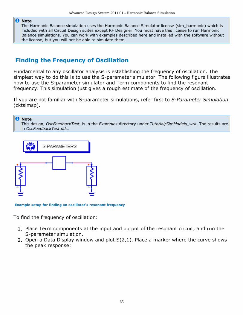
Advanced Design System 2011.01 - Harmonic Balance Simulation
65
NoteThe Harmonic Balance simulation uses the Harmonic Balance Simulator license (sim_harmonic) which isincluded with all Circuit Design suites except RF Designer. You must have this license to run HarmonicBalance simulations. You can work with examples described here and installed with the software withoutthe license, but you will not be able to simulate them.
Finding the Frequency of Oscillation
Fundamental to any oscillator analysis is establishing the frequency of oscillation. Thesimplest way to do this is to use the S-parameter simulator. The following figure illustrateshow to use the S-parameter simulator and Term components to find the resonantfrequency. This simulation just gives a rough estimate of the frequency of oscillation.
If you are not familiar with S-parameter simulations, refer first to S-Parameter Simulation(cktsimsp).
NoteThis design, OscFeedbackTest, is in the Examples directory under Tutorial/SimModels_wrk. The results arein OscFeedbackTest.dds.
Example setup for finding an oscillator's resonant frequency
To find the frequency of oscillation:
Place Term components at the input and output of the resonant circuit, and run the1.S-parameter simulation.Open a Data Display window and plot S(2,1). Place a marker where the curve shows2.the peak response:
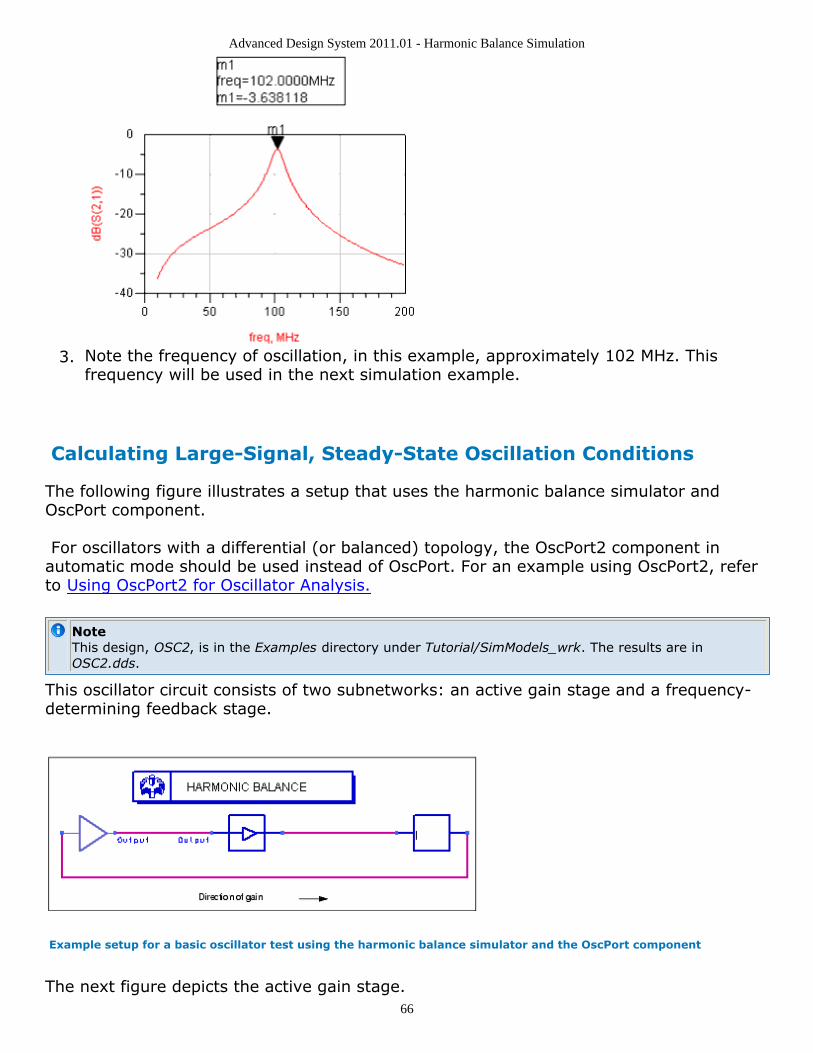
Advanced Design System 2011.01 - Harmonic Balance Simulation
66
Note the frequency of oscillation, in this example, approximately 102 MHz. This3.frequency will be used in the next simulation example.
Calculating Large-Signal, Steady-State Oscillation Conditions
The following figure illustrates a setup that uses the harmonic balance simulator andOscPort component.
For oscillators with a differential (or balanced) topology, the OscPort2 component inautomatic mode should be used instead of OscPort. For an example using OscPort2, referto Using OscPort2 for Oscillator Analysis.
NoteThis design, OSC2, is in the Examples directory under Tutorial/SimModels_wrk. The results are inOSC2.dds.
This oscillator circuit consists of two subnetworks: an active gain stage and a frequency-determining feedback stage.
Example setup for a basic oscillator test using the harmonic balance simulator and the OscPort component
The next figure depicts the active gain stage.
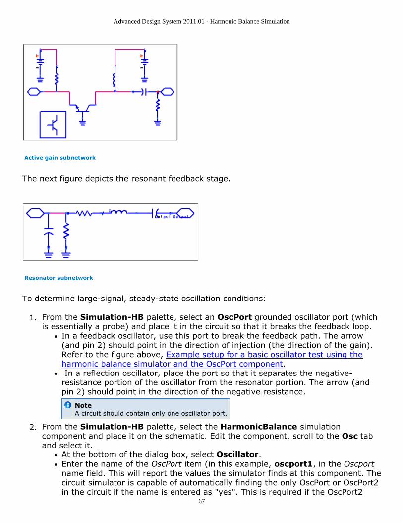
Advanced Design System 2011.01 - Harmonic Balance Simulation
67
Active gain subnetwork
The next figure depicts the resonant feedback stage.
Resonator subnetwork
To determine large-signal, steady-state oscillation conditions:
From the Simulation-HB palette, select an OscPort grounded oscillator port (which1.is essentially a probe) and place it in the circuit so that it breaks the feedback loop.
In a feedback oscillator, use this port to break the feedback path. The arrow(and pin 2) should point in the direction of injection (the direction of the gain).Refer to the figure above, Example setup for a basic oscillator test using theharmonic balance simulator and the OscPort component. In a reflection oscillator, place the port so that it separates the negative-resistance portion of the oscillator from the resonator portion. The arrow (andpin 2) should point in the direction of the negative resistance.
NoteA circuit should contain only one oscillator port.
From the Simulation-HB palette, select the HarmonicBalance simulation2.component and place it on the schematic. Edit the component, scroll to the Osc taband select it.
At the bottom of the dialog box, select Oscillator.Enter the name of the OscPort item (in this example, oscport1, in the Oscportname field. This will report the values the simulator finds at this component. Thecircuit simulator is capable of automatically finding the only OscPort or OscPort2in the circuit if the name is entered as "yes". This is required if the OscPort2
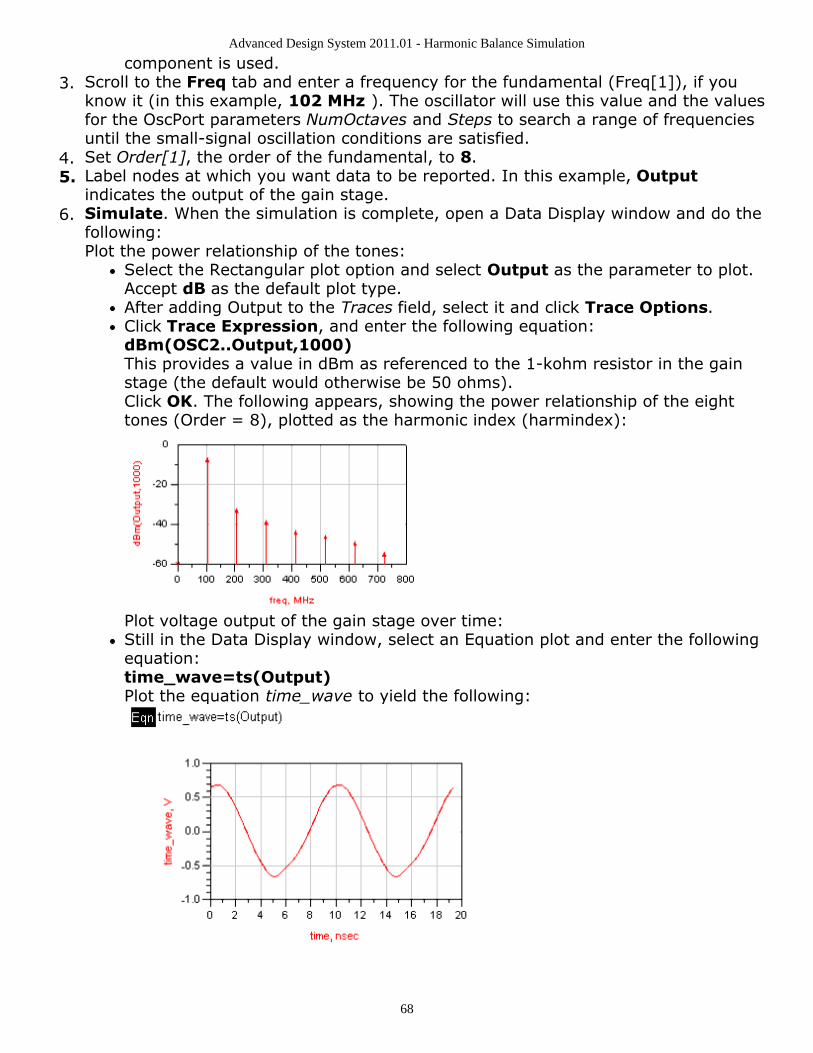
Advanced Design System 2011.01 - Harmonic Balance Simulation
68
component is used.Scroll to the Freq tab and enter a frequency for the fundamental (Freq[1]), if you3.know it (in this example, 102 MHz ). The oscillator will use this value and the valuesfor the OscPort parameters NumOctaves and Steps to search a range of frequenciesuntil the small-signal oscillation conditions are satisfied.Set Order[1], the order of the fundamental, to 8.4.Label nodes at which you want data to be reported. In this example, Output5.indicates the output of the gain stage.Simulate. When the simulation is complete, open a Data Display window and do the6.following:Plot the power relationship of the tones:
Select the Rectangular plot option and select Output as the parameter to plot.Accept dB as the default plot type.After adding Output to the Traces field, select it and click Trace Options.Click Trace Expression, and enter the following equation:dBm(OSC2..Output,1000)This provides a value in dBm as referenced to the 1-kohm resistor in the gainstage (the default would otherwise be 50 ohms).Click OK. The following appears, showing the power relationship of the eighttones (Order = 8), plotted as the harmonic index (harmindex):
Plot voltage output of the gain stage over time:Still in the Data Display window, select an Equation plot and enter the followingequation:time_wave=ts(Output)Plot the equation time_wave to yield the following:
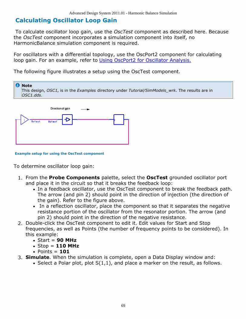
Advanced Design System 2011.01 - Harmonic Balance Simulation
69
Calculating Oscillator Loop Gain
To calculate oscillator loop gain, use the OscTest component as described here. Becausethe OscTest component incorporates a simulation component into itself, noHarmonicBalance simulation component is required.
For oscillators with a differential topology, use the OscPort2 component for calculatingloop gain. For an example, refer to Using OscPort2 for Oscillator Analysis.
The following figure illustrates a setup using the OscTest component.
NoteThis design, OSC1, is in the Examples directory under Tutorial/SimModels_wrk. The results are inOSC1.dds.
Example setup for using the OscTest component
To determine oscillator loop gain:
From the Probe Components palette, select the OscTest grounded oscillator port1.and place it in the circuit so that it breaks the feedback loop:
In a feedback oscillator, use the OscTest component to break the feedback path.The arrow (and pin 2) should point in the direction of injection (the direction ofthe gain). Refer to the figure above. In a reflection oscillator, place the component so that it separates the negativeresistance portion of the oscillator from the resonator portion. The arrow (andpin 2) should point in the direction of the negative resistance.
Double-click the OscTest component to edit it. Edit values for Start and Stop2.frequencies, as well as Points (the number of frequency points to be considered). Inthis example:
Start = 90 MHzStop = 110 MHzPoints = 101
Simulate. When the simulation is complete, open a Data Display window and:3.Select a Polar plot, plot S(1,1), and place a marker on the result, as follows.
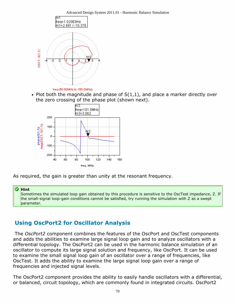
Advanced Design System 2011.01 - Harmonic Balance Simulation
70
Plot both the magnitude and phase of S(1,1), and place a marker directly overthe zero crossing of the phase plot (shown next).
As required, the gain is greater than unity at the resonant frequency.
HintSometimes the simulated loop gain obtained by this procedure is sensitive to the OscTest impedance, Z. Ifthe small-signal loop-gain conditions cannot be satisfied, try running the simulation with Z as a sweptparameter.
Using OscPort2 for Oscillator Analysis
The OscPort2 component combines the features of the OscPort and OscTest componentsand adds the abilities to examine large signal loop gain and to analyze oscillators with adifferential topology. The OscPort2 can be used in the harmonic balance simulation of anoscillator to compute its large signal solution and frequency, like OscPort. It can be usedto examine the small signal loop gain of an oscillator over a range of frequencies, likeOscTest. It adds the ability to examine the large signal loop gain over a range offrequencies and injected signal levels.
The OscPort2 component provides the ability to easily handle oscillators with a differential,or balanced, circuit topology, which are commonly found in integrated circuits. OscPort2
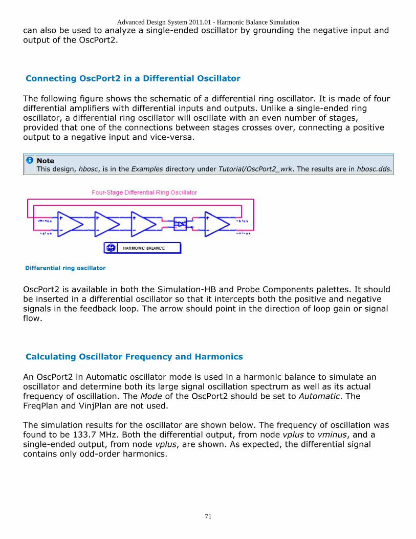
Advanced Design System 2011.01 - Harmonic Balance Simulation
71
can also be used to analyze a single-ended oscillator by grounding the negative input andoutput of the OscPort2.
Connecting OscPort2 in a Differential Oscillator
The following figure shows the schematic of a differential ring oscillator. It is made of fourdifferential amplifiers with differential inputs and outputs. Unlike a single-ended ringoscillator, a differential ring oscillator will oscillate with an even number of stages,provided that one of the connections between stages crosses over, connecting a positiveoutput to a negative input and vice-versa.
NoteThis design, hbosc, is in the Examples directory under Tutorial/OscPort2_wrk. The results are in hbosc.dds.
Differential ring oscillator
OscPort2 is available in both the Simulation-HB and Probe Components palettes. It shouldbe inserted in a differential oscillator so that it intercepts both the positive and negativesignals in the feedback loop. The arrow should point in the direction of loop gain or signalflow.
Calculating Oscillator Frequency and Harmonics
An OscPort2 in Automatic oscillator mode is used in a harmonic balance to simulate anoscillator and determine both its large signal oscillation spectrum as well as its actualfrequency of oscillation. The Mode of the OscPort2 should be set to Automatic. TheFreqPlan and VinjPlan are not used.
The simulation results for the oscillator are shown below. The frequency of oscillation wasfound to be 133.7 MHz. Both the differential output, from node vplus to vminus, and asingle-ended output, from node vplus, are shown. As expected, the differential signalcontains only odd-order harmonics.
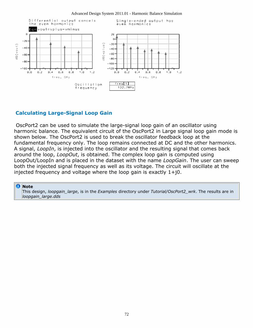
Advanced Design System 2011.01 - Harmonic Balance Simulation
72
Calculating Large-Signal Loop Gain
OscPort2 can be used to simulate the large-signal loop gain of an oscillator usingharmonic balance. The equivalent circuit of the OscPort2 in Large signal loop gain mode isshown below. The OscPort2 is used to break the oscillator feedback loop at thefundamental frequency only. The loop remains connected at DC and the other harmonics.A signal, LoopIn, is injected into the oscillator and the resulting signal that comes backaround the loop, LoopOut, is obtained. The complex loop gain is computed usingLoopOut/LoopIn and is placed in the dataset with the name LoopGain. The user can sweepboth the injected signal frequency as well as its voltage. The circuit will oscillate at theinjected frequency and voltage where the loop gain is exactly 1+j0.
NoteThis design, loopgain_large, is in the Examples directory under Tutorial/OscPort2_wrk. The results are inloopgain_large.dds
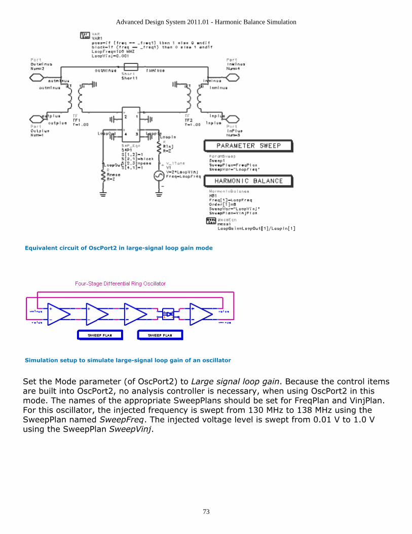
Advanced Design System 2011.01 - Harmonic Balance Simulation
73
Equivalent circuit of OscPort2 in large-signal loop gain mode
Simulation setup to simulate large-signal loop gain of an oscillator
Set the Mode parameter (of OscPort2) to Large signal loop gain. Because the control itemsare built into OscPort2, no analysis controller is necessary, when using OscPort2 in thismode. The names of the appropriate SweepPlans should be set for FreqPlan and VinjPlan.For this oscillator, the injected frequency is swept from 130 MHz to 138 MHz using theSweepPlan named SweepFreq. The injected voltage level is swept from 0.01 V to 1.0 Vusing the SweepPlan SweepVinj.
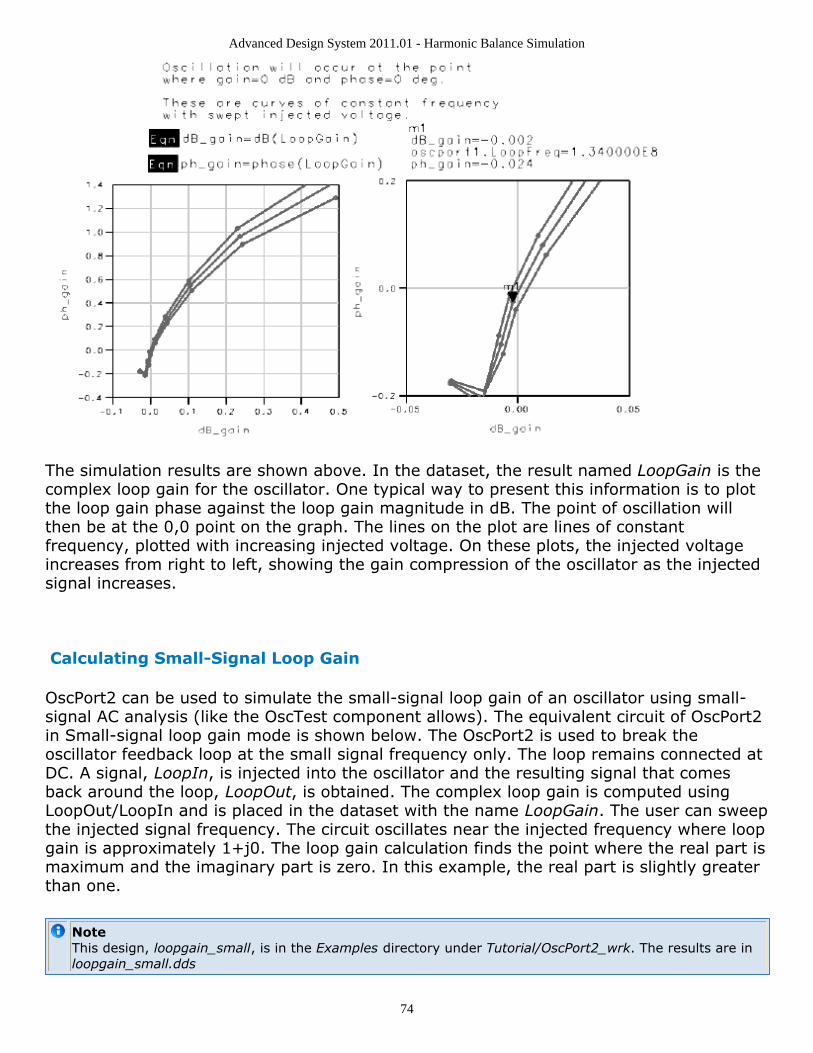
Advanced Design System 2011.01 - Harmonic Balance Simulation
74
The simulation results are shown above. In the dataset, the result named LoopGain is thecomplex loop gain for the oscillator. One typical way to present this information is to plotthe loop gain phase against the loop gain magnitude in dB. The point of oscillation willthen be at the 0,0 point on the graph. The lines on the plot are lines of constantfrequency, plotted with increasing injected voltage. On these plots, the injected voltageincreases from right to left, showing the gain compression of the oscillator as the injectedsignal increases.
Calculating Small-Signal Loop Gain
OscPort2 can be used to simulate the small-signal loop gain of an oscillator using small-signal AC analysis (like the OscTest component allows). The equivalent circuit of OscPort2in Small-signal loop gain mode is shown below. The OscPort2 is used to break theoscillator feedback loop at the small signal frequency only. The loop remains connected atDC. A signal, LoopIn, is injected into the oscillator and the resulting signal that comesback around the loop, LoopOut, is obtained. The complex loop gain is computed usingLoopOut/LoopIn and is placed in the dataset with the name LoopGain. The user can sweepthe injected signal frequency. The circuit oscillates near the injected frequency where loopgain is approximately 1+j0. The loop gain calculation finds the point where the real part ismaximum and the imaginary part is zero. In this example, the real part is slightly greaterthan one.
NoteThis design, loopgain_small, is in the Examples directory under Tutorial/OscPort2_wrk. The results are inloopgain_small.dds
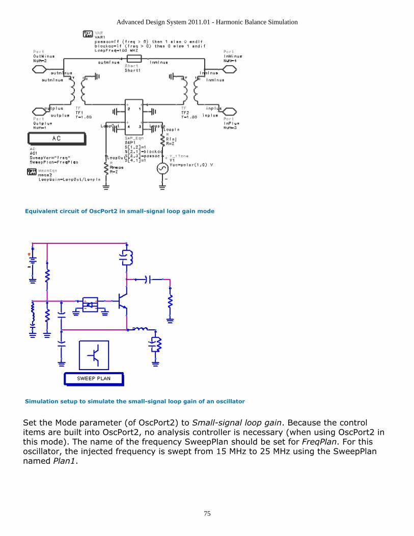
Advanced Design System 2011.01 - Harmonic Balance Simulation
75
Equivalent circuit of OscPort2 in small-signal loop gain mode
Simulation setup to simulate the small-signal loop gain of an oscillator
Set the Mode parameter (of OscPort2) to Small-signal loop gain. Because the controlitems are built into OscPort2, no analysis controller is necessary (when using OscPort2 inthis mode). The name of the frequency SweepPlan should be set for FreqPlan. For thisoscillator, the injected frequency is swept from 15 MHz to 25 MHz using the SweepPlannamed Plan1.
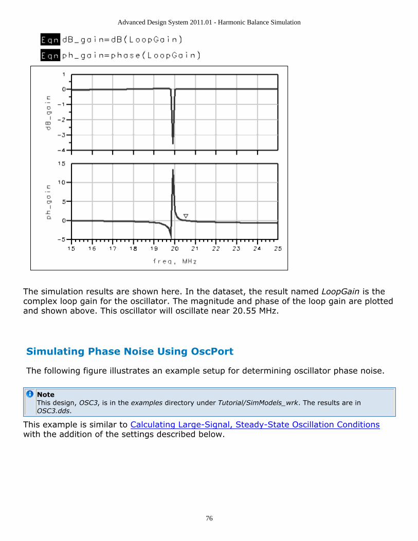
Advanced Design System 2011.01 - Harmonic Balance Simulation
76
The simulation results are shown here. In the dataset, the result named LoopGain is thecomplex loop gain for the oscillator. The magnitude and phase of the loop gain are plottedand shown above. This oscillator will oscillate near 20.55 MHz.
Simulating Phase Noise Using OscPort
The following figure illustrates an example setup for determining oscillator phase noise.
NoteThis design, OSC3, is in the examples directory under Tutorial/SimModels_wrk. The results are inOSC3.dds.
This example is similar to Calculating Large-Signal, Steady-State Oscillation Conditionswith the addition of the settings described below.
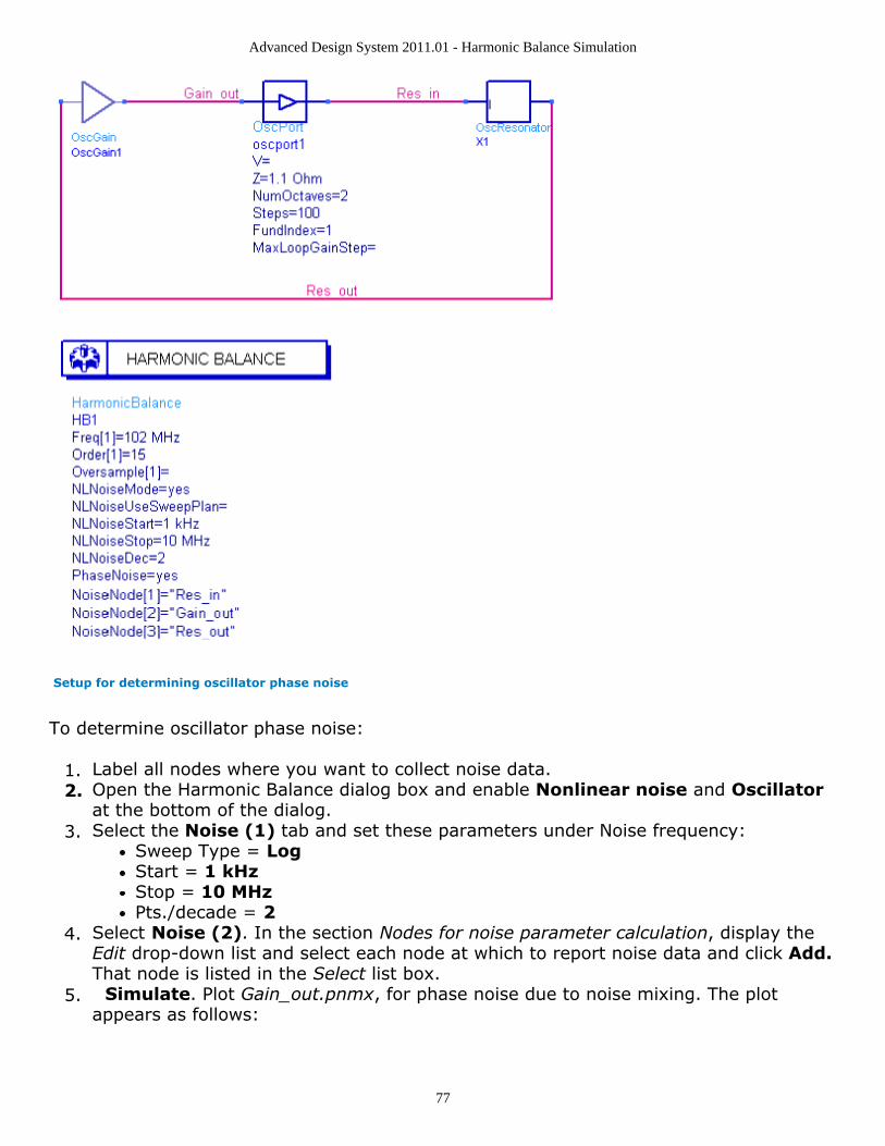
Advanced Design System 2011.01 - Harmonic Balance Simulation
77
Setup for determining oscillator phase noise
To determine oscillator phase noise:
Label all nodes where you want to collect noise data.1.Open the Harmonic Balance dialog box and enable Nonlinear noise and Oscillator2.at the bottom of the dialog.Select the Noise (1) tab and set these parameters under Noise frequency:3.
Sweep Type = LogStart = 1 kHzStop = 10 MHzPts./decade = 2
Select Noise (2). In the section Nodes for noise parameter calculation, display the4.Edit drop-down list and select each node at which to report noise data and click Add.That node is listed in the Select list box. Simulate. Plot Gain_out.pnmx, for phase noise due to noise mixing. The plot5.appears as follows:
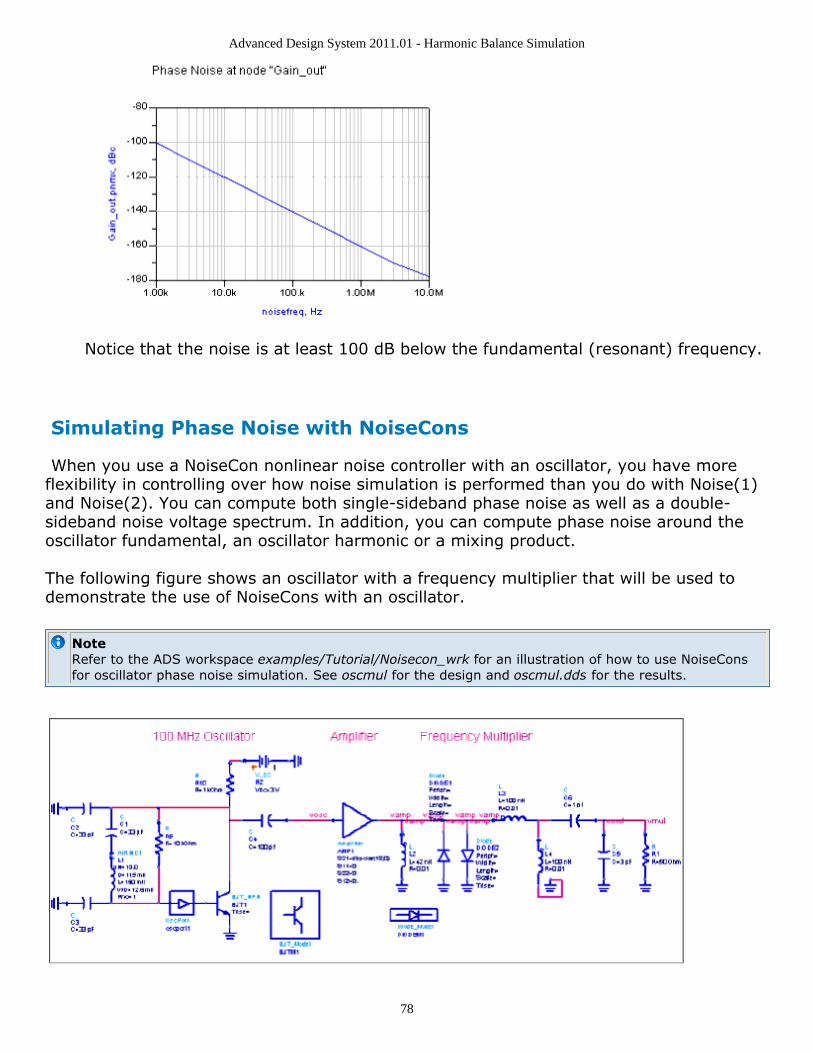
Advanced Design System 2011.01 - Harmonic Balance Simulation
78
Notice that the noise is at least 100 dB below the fundamental (resonant) frequency.
Simulating Phase Noise with NoiseCons
When you use a NoiseCon nonlinear noise controller with an oscillator, you have moreflexibility in controlling over how noise simulation is performed than you do with Noise(1)and Noise(2). You can compute both single-sideband phase noise as well as a double-sideband noise voltage spectrum. In addition, you can compute phase noise around theoscillator fundamental, an oscillator harmonic or a mixing product.
The following figure shows an oscillator with a frequency multiplier that will be used todemonstrate the use of NoiseCons with an oscillator.
NoteRefer to the ADS workspace examples/Tutorial/Noisecon_wrk for an illustration of how to use NoiseConsfor oscillator phase noise simulation. See oscmul for the design and oscmul.dds for the results.
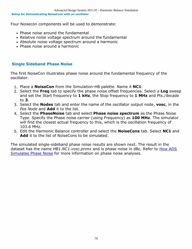
Advanced Design System 2011.01 - Harmonic Balance Simulation
79
Setup for demonstrating NoiseCons with an oscillator
Four Noisecon components will be used to demonstrate:
Phase noise around the fundamentalRelative noise voltage spectrum around the fundamentalAbsolute noise voltage spectrum around a harmonicPhase noise around a harmonic
Single Sideband Phase Noise
The first NoiseCon illustrates phase noise around the fundamental frequency of theoscillator.
Place a NoiseCon from the Simulation-HB palette. Name it NC1.1.Select the Freq tab to specify the phase noise offset frequencies. Select a Log sweep2.and set the Start frequency to 1 kHz, the Stop frequency to 1 MHz and Pts./decadeto 3.Select the Nodes tab and enter the name of the oscillator output node, vosc, in the3.Pos Node and Add it to the list.Select the PhaseNoise tab and select Phase noise spectrum as the Phase Noise4.Type. Specify the Phase noise carrier (using Frequency) as 100 MHz. The simulatorwill find the closest actual frequency to this, which is the oscillation frequency of103.6 MHz.Edit the Harmonic Balance controller and select the NoiseCons tab. Select NC1 and5.Add it to the list of NoiseCons to be simulated.
The simulated single-sideband phase noise results are shown next. The result in thedataset has the name HB1.NC1.vosc.pnmx and is phase noise in dBc. Refer to How ADSSimulates Phase Noise for more information on phase noise analyses.
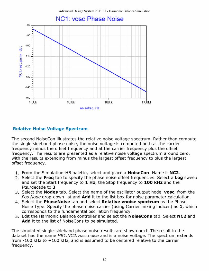
Advanced Design System 2011.01 - Harmonic Balance Simulation
80
Relative Noise Voltage Spectrum
The second NoiseCon illustrates the relative noise voltage spectrum. Rather than computethe single sideband phase noise, the noise voltage is computed both at the carrierfrequency minus the offset frequency and at the carrier frequency plus the offsetfrequency. The results are presented as a relative noise voltage spectrum around zero,with the results extending from minus the largest offset frequency to plus the largestoffset frequency.
From the Simulation-HB palette, select and place a NoiseCon. Name it NC2.1.Select the Freq tab to specify the phase noise offset frequencies. Select a Log sweep2.and set the Start frequency to 1 Hz, the Stop frequency to 100 kHz and thePts./decade to 3.Select the Nodes tab. Select the name of the oscillator output node, vosc, from the3.Pos Node drop-down list and Add it to the list box for noise parameter calculation.Select the PhaseNoise tab and select Relative vnoise spectrum as the Phase4.Noise Type. Specify the phase noise carrier (using Carrier mixing indices) as 1, whichcorresponds to the fundamental oscillation frequency.Edit the Harmonic Balance controller and select the NoiseCons tab. Select NC2 and5.Add it to the list of NoiseCons to be simulated.
The simulated single-sideband phase noise results are shown next. The result in thedataset has the name HB1.NC2.vosc.noise and is a noise voltage. The spectrum extendsfrom -100 kHz to +100 kHz, and is assumed to be centered relative to the carrierfrequency.
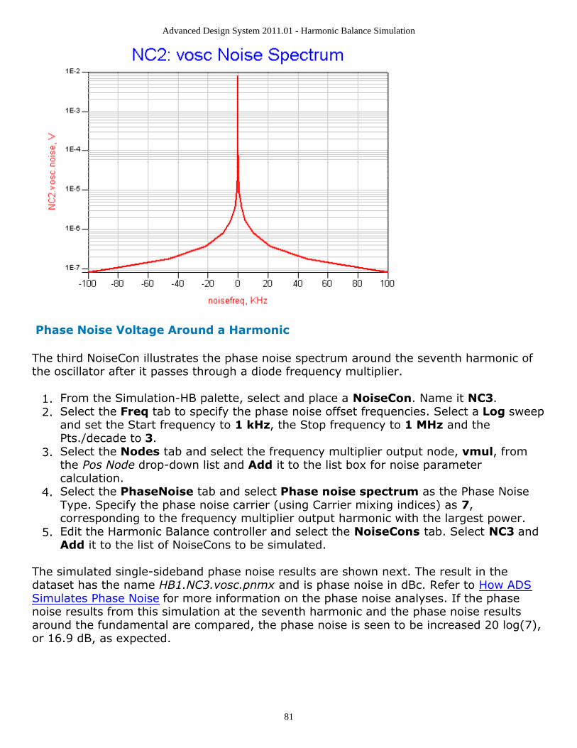
Advanced Design System 2011.01 - Harmonic Balance Simulation
81
Phase Noise Voltage Around a Harmonic
The third NoiseCon illustrates the phase noise spectrum around the seventh harmonic ofthe oscillator after it passes through a diode frequency multiplier.
From the Simulation-HB palette, select and place a NoiseCon. Name it NC3.1.Select the Freq tab to specify the phase noise offset frequencies. Select a Log sweep2.and set the Start frequency to 1 kHz, the Stop frequency to 1 MHz and thePts./decade to 3.Select the Nodes tab and select the frequency multiplier output node, vmul, from3.the Pos Node drop-down list and Add it to the list box for noise parametercalculation.Select the PhaseNoise tab and select Phase noise spectrum as the Phase Noise4.Type. Specify the phase noise carrier (using Carrier mixing indices) as 7,corresponding to the frequency multiplier output harmonic with the largest power.Edit the Harmonic Balance controller and select the NoiseCons tab. Select NC3 and5.Add it to the list of NoiseCons to be simulated.
The simulated single-sideband phase noise results are shown next. The result in thedataset has the name HB1.NC3.vosc.pnmx and is phase noise in dBc. Refer to How ADSSimulates Phase Noise for more information on the phase noise analyses. If the phasenoise results from this simulation at the seventh harmonic and the phase noise resultsaround the fundamental are compared, the phase noise is seen to be increased 20 log(7),or 16.9 dB, as expected.
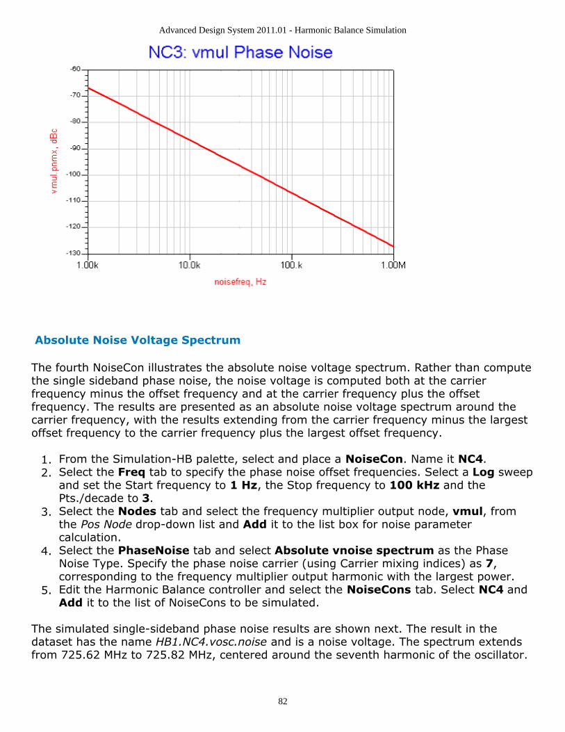
Advanced Design System 2011.01 - Harmonic Balance Simulation
82
Absolute Noise Voltage Spectrum
The fourth NoiseCon illustrates the absolute noise voltage spectrum. Rather than computethe single sideband phase noise, the noise voltage is computed both at the carrierfrequency minus the offset frequency and at the carrier frequency plus the offsetfrequency. The results are presented as an absolute noise voltage spectrum around thecarrier frequency, with the results extending from the carrier frequency minus the largestoffset frequency to the carrier frequency plus the largest offset frequency.
From the Simulation-HB palette, select and place a NoiseCon. Name it NC4.1.Select the Freq tab to specify the phase noise offset frequencies. Select a Log sweep2.and set the Start frequency to 1 Hz, the Stop frequency to 100 kHz and thePts./decade to 3.Select the Nodes tab and select the frequency multiplier output node, vmul, from3.the Pos Node drop-down list and Add it to the list box for noise parametercalculation.Select the PhaseNoise tab and select Absolute vnoise spectrum as the Phase4.Noise Type. Specify the phase noise carrier (using Carrier mixing indices) as 7,corresponding to the frequency multiplier output harmonic with the largest power.Edit the Harmonic Balance controller and select the NoiseCons tab. Select NC4 and5.Add it to the list of NoiseCons to be simulated.
The simulated single-sideband phase noise results are shown next. The result in thedataset has the name HB1.NC4.vosc.noise and is a noise voltage. The spectrum extendsfrom 725.62 MHz to 725.82 MHz, centered around the seventh harmonic of the oscillator.
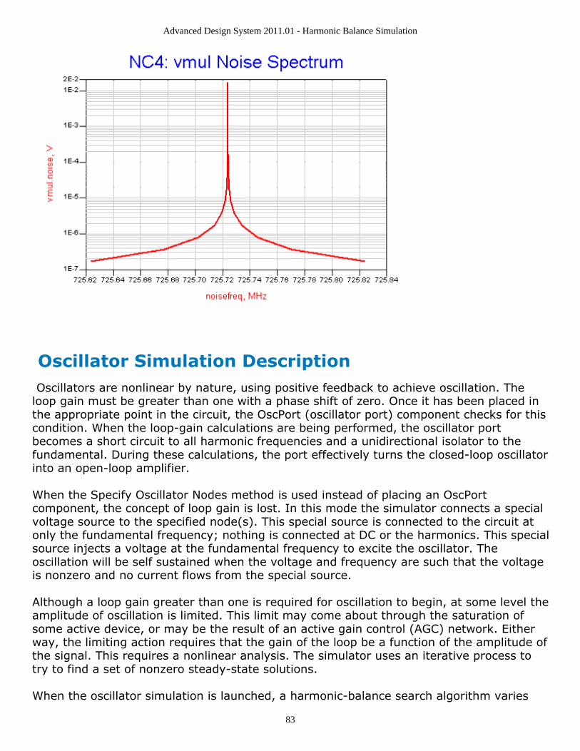
Advanced Design System 2011.01 - Harmonic Balance Simulation
83
Oscillator Simulation Description Oscillators are nonlinear by nature, using positive feedback to achieve oscillation. Theloop gain must be greater than one with a phase shift of zero. Once it has been placed inthe appropriate point in the circuit, the OscPort (oscillator port) component checks for thiscondition. When the loop-gain calculations are being performed, the oscillator portbecomes a short circuit to all harmonic frequencies and a unidirectional isolator to thefundamental. During these calculations, the port effectively turns the closed-loop oscillatorinto an open-loop amplifier.
When the Specify Oscillator Nodes method is used instead of placing an OscPortcomponent, the concept of loop gain is lost. In this mode the simulator connects a specialvoltage source to the specified node(s). This special source is connected to the circuit atonly the fundamental frequency; nothing is connected at DC or the harmonics. This specialsource injects a voltage at the fundamental frequency to excite the oscillator. Theoscillation will be self sustained when the voltage and frequency are such that the voltageis nonzero and no current flows from the special source.
Although a loop gain greater than one is required for oscillation to begin, at some level theamplitude of oscillation is limited. This limit may come about through the saturation ofsome active device, or may be the result of an active gain control (AGC) network. Eitherway, the limiting action requires that the gain of the loop be a function of the amplitude ofthe signal. This requires a nonlinear analysis. The simulator uses an iterative process totry to find a set of nonzero steady-state solutions.
When the oscillator simulation is launched, a harmonic-balance search algorithm varies
Advanced Design System 2011.01 - Harmonic Balance Simulation
84
the operating frequency to find the oscillation frequency, as well as the final operatingfrequency and power levels, of the oscillator circuit.
Note Power levels are computed by means of a reference impedance value. However, because this valuetypically does not represent your circuit's impedance, the power levels may not be physically meaningful.For example, in a high-impedance oscillator, the simulation power levels may be much greater than thepower the oscillator can actually deliver to its load.
The simulator performs a fully automated search for the oscillator's operatingcharacteristics. The automated search involves:
Searching for a frequency where the circuit satisfies the linear oscillation condition.Searching for a frequency and power such that the oscillator's open-loop gain is atunity magnitude and zero phase angle (within a given tolerance).A full closed-loop harmonic balance analysis in which frequency and oscillator powerare further refined to a more exact solution.
Performing VCO Tuning
VCO tuning is accomplished by performing an oscillator simulation in conjunction with aswept variable analysis (refer to Parameter Sweeps and Sweep Plans (cktsim)). Thesimulator performs a separate oscillator analysis for each swept variable value, thenattempts to find the actual oscillation condition for each value. After the analysis iscomplete, you can display the frequency of oscillation and the output power of thatfrequency as a function of, for example, the swept variable.
You should not sweep a variable in large steps, because that may snap the algorithm outof the vicinity of the prior oscillation condition, resulting in a convergence failure.
Measuring Oscillator Loop Gain
A quick and efficient way to ensure that the network meets the necessary conditions foroscillation is to use the OscTest component to verify whether the linear oscillationconditions are satisfied. OscTest performs a small-signal loop gain analysis on theoscillator. It does the initial analysis that is performed by the OscPort component, and itacts like a signal source, load, and ideal circulator. The impedance of the source and loadare the same, and are set via the Z-parameter on the OscTest component. For someoscillators, the loop gain and phase shift vary with this Z-parameter, so it is sometimes agood idea to check the loop gain and phase shift versus frequency for different values ofthe Z-parameter. The results of a simulation with an OscTest component are the small-signal open loop gain and phase shift, as a function of frequency. Generally, the circuit willoscillate if the open loop gain satisfies
|Gl| > 1, Im (Gl ) = 0
Advanced Design System 2011.01 - Harmonic Balance Simulation
85
or equivalently, where the output impedance (Zout) satisfies
Re (Zout) < 0, Im(Zout) = 0
For a more rigorous description of the oscillation conditions that must be satisfied, refer tothe oscillator component descriptions in Introduction to Circuit Components (ccsim).
NoteBecause the control items are built into OscTest, no analysis controller is necessary.
In addition, an example of this type of analysis can be found in the example file/examples/Tutorial/LearnOsc_wrk/OscTest_VCO. The application note, PN 85150-4Simulating Noise in Nonlinear Circuits Using MDS/RFDS, provides further informationabout determining the expected frequency of oscillation for an oscillator, including adescription of a method that does not use the OscTest component. This application note isaccessible from the Agilent EEsof website.
After performing the simulations with OscTest and finding the potential frequency ofoscillation, OscTest can be replaced with an OscPort and oscillator harmonic balancesimulations can then be run.
It is important to note that an OscTest analysis is not an accurate way to determine theoscillation frequency, nor does it help determine the operating power levels of theoscillator. During oscillation, reactances within the device change considerably, causingfrequency shifts not predicted by the linear simulation.
A large-signal nonlinear analysis accounts for the variations in device reactances andprovides a way to determine the oscillation frequency with far greater accuracy. It alsoprovides information on the output power level of the oscillator, output power spectrum,and voltage and current waveforms.
Consider the operation of a negative-resistance oscillator from a point in the networkbetween the resonating circuit and the nonlinear device:
Ambient noise usually provides the initial stimulus. When a small voltage disturbanceat the appropriate frequency is presented at this node, it encounters negativeresistance at the device and reflects back to the resonator with a greater magnitude.The resonator reflects the signal, which experiences some loss as it propagatesthrough the circuit. As long as the negative resistance of the device is sufficient toexceed the losses in the circuit, the stimulus signal continues to grow.At some point, the magnitude of the signal becomes sufficient to reduce the negativeresistance of the device.Steady state is reached when the magnitude of the signal causes the negativeresistance and the loss effects to be balanced. Nonlinearities in the device willgenerate harmonics, which also reach steady-state values.
There are two unknowns in the process of simulating an oscillator:
Amplitude of the injection/feedback signal
Advanced Design System 2011.01 - Harmonic Balance Simulation
86
Frequency of oscillation
The injection amplitude must be adjusted and applied over a range of frequencies until theoscillation conditions are met at one of the frequencies. Only then is the oscillator'ssteady-state operating point obtained.
Phase Noise Simulation Description An oscillator phase noise analysis computes the noise sidebands of the oscillator carrierfrequency as well as:
Normal frequency conversionAmplitude-noise-to-frequency-noise conversionFrequency translation of noise, caused by component nonlinearities in the presenceof large-signal oscillator signals. Upconverted flicker noise is a commonly observedeffect.Bias changes due to the oscillator signals. Any shift in DC bias that occurs in thepresence of the oscillation waveforms is taken into account. This bias-shift calculationis needed for accurate calculations of nonlinear device noise.
The results from the phase noise analysis have .pnmx (phase noise, in dBc/Hz) and .anmx(AM noise, in dBc/Hz) appended to the selected node name(s).
NoteMost of the nonlinear devices in the semiconductor libraries do not have stable 1/f noise parameters.Instead, noise sources must be added to model the 1/f noise.
How ADS Simulates Phase Noise
Phase noise in an oscillator can be analyzed from small-signal mixing of noise. The small-signal mixing of noise comes from the nonlinear behavior of the oscillator, where noisemixes with the oscillator signal and harmonics to mix to sideband frequencies on eitherside of the oscillator signal.
The phase noise computed is available to the user directly in dBc. Assuming there is anode labeled vout for which phase noise is to be computed, the following variables areavailable for use in a data display following a phase noise analysis.
hb_noise.vout.pnmx (phase noise (in dBc) from mixing analysis)
hb_noise.vout.anmx (AM noise in (dBc) from mixing analysis)
To model oscillator phase noise with a noise mixing analysis, the noise at the sidebands
on either side of the carrier are obtained from a small-signal mixer analysis
where noise sources mix with the oscillator large signals to produce noise
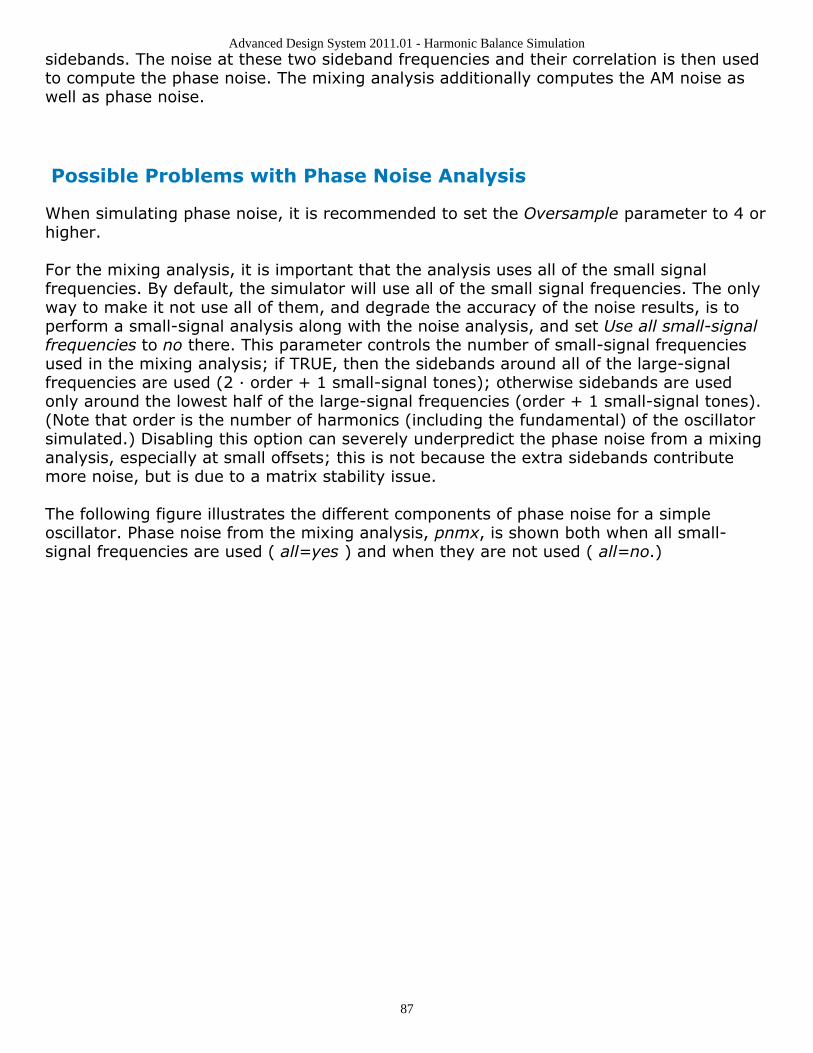
Advanced Design System 2011.01 - Harmonic Balance Simulation
87
sidebands. The noise at these two sideband frequencies and their correlation is then usedto compute the phase noise. The mixing analysis additionally computes the AM noise aswell as phase noise.
Possible Problems with Phase Noise Analysis
When simulating phase noise, it is recommended to set the Oversample parameter to 4 orhigher.
For the mixing analysis, it is important that the analysis uses all of the small signalfrequencies. By default, the simulator will use all of the small signal frequencies. The onlyway to make it not use all of them, and degrade the accuracy of the noise results, is toperform a small-signal analysis along with the noise analysis, and set Use all small-signalfrequencies to no there. This parameter controls the number of small-signal frequenciesused in the mixing analysis; if TRUE, then the sidebands around all of the large-signalfrequencies are used (2 · order + 1 small-signal tones); otherwise sidebands are usedonly around the lowest half of the large-signal frequencies (order + 1 small-signal tones).(Note that order is the number of harmonics (including the fundamental) of the oscillatorsimulated.) Disabling this option can severely underpredict the phase noise from a mixinganalysis, especially at small offsets; this is not because the extra sidebands contributemore noise, but is due to a matrix stability issue.
The following figure illustrates the different components of phase noise for a simpleoscillator. Phase noise from the mixing analysis, pnmx, is shown both when all small-signal frequencies are used ( all=yes ) and when they are not used ( all=no.)
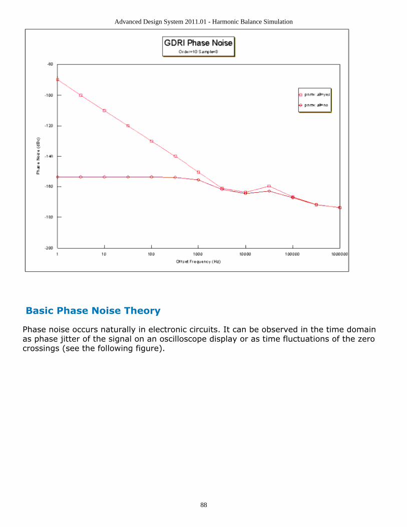
Advanced Design System 2011.01 - Harmonic Balance Simulation
88
Basic Phase Noise Theory
Phase noise occurs naturally in electronic circuits. It can be observed in the time domainas phase jitter of the signal on an oscilloscope display or as time fluctuations of the zerocrossings (see the following figure).
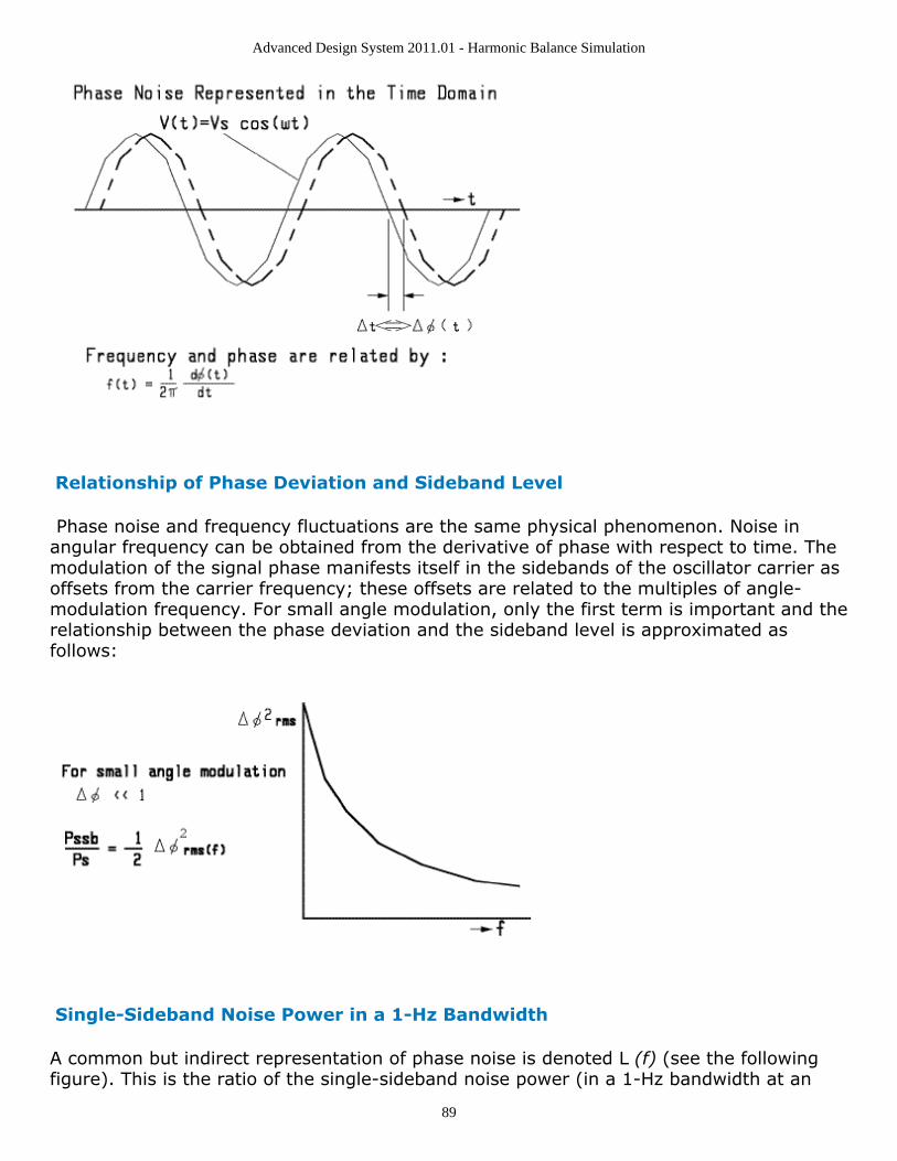
Advanced Design System 2011.01 - Harmonic Balance Simulation
89
Relationship of Phase Deviation and Sideband Level
Phase noise and frequency fluctuations are the same physical phenomenon. Noise inangular frequency can be obtained from the derivative of phase with respect to time. Themodulation of the signal phase manifests itself in the sidebands of the oscillator carrier asoffsets from the carrier frequency; these offsets are related to the multiples of angle-modulation frequency. For small angle modulation, only the first term is important and therelationship between the phase deviation and the sideband level is approximated asfollows:
Single-Sideband Noise Power in a 1-Hz Bandwidth
A common but indirect representation of phase noise is denoted L (f) (see the followingfigure). This is the ratio of the single-sideband noise power (in a 1-Hz bandwidth at an
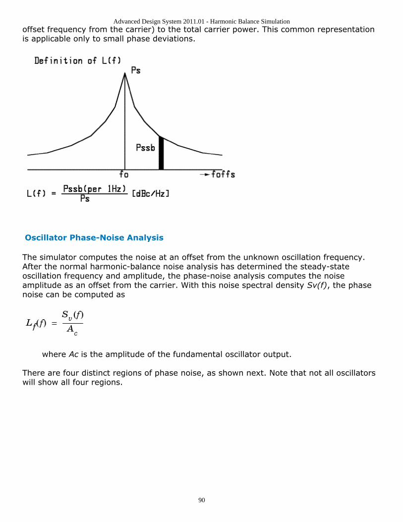
Advanced Design System 2011.01 - Harmonic Balance Simulation
90
offset frequency from the carrier) to the total carrier power. This common representationis applicable only to small phase deviations.
Oscillator Phase-Noise Analysis
The simulator computes the noise at an offset from the unknown oscillation frequency.After the normal harmonic-balance noise analysis has determined the steady-stateoscillation frequency and amplitude, the phase-noise analysis computes the noiseamplitude as an offset from the carrier. With this noise spectral density Sv(f), the phasenoise can be computed as
where Ac is the amplitude of the fundamental oscillator output.
There are four distinct regions of phase noise, as shown next. Note that not all oscillatorswill show all four regions.
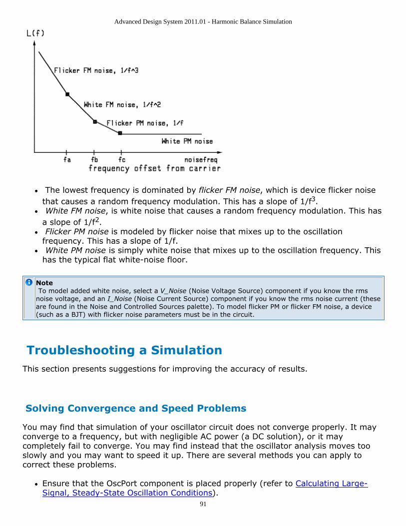
Advanced Design System 2011.01 - Harmonic Balance Simulation
91
The lowest frequency is dominated by flicker FM noise, which is device flicker noisethat causes a random frequency modulation. This has a slope of 1/f3. White FM noise, is white noise that causes a random frequency modulation. This hasa slope of 1/f2. Flicker PM noise is modeled by flicker noise that mixes up to the oscillationfrequency. This has a slope of 1/f. White PM noise is simply white noise that mixes up to the oscillation frequency. Thishas the typical flat white-noise floor.
Note To model added white noise, select a V_Noise (Noise Voltage Source) component if you know the rmsnoise voltage, and an I_Noise (Noise Current Source) component if you know the rms noise current (theseare found in the Noise and Controlled Sources palette). To model flicker PM or flicker FM noise, a device(such as a BJT) with flicker noise parameters must be in the circuit.
Troubleshooting a SimulationThis section presents suggestions for improving the accuracy of results.
Solving Convergence and Speed Problems
You may find that simulation of your oscillator circuit does not converge properly. It mayconverge to a frequency, but with negligible AC power (a DC solution), or it maycompletely fail to converge. You may find instead that the oscillator analysis moves tooslowly and you may want to speed it up. There are several methods you can apply tocorrect these problems.
Ensure that the OscPort component is placed properly (refer to Calculating Large-Signal, Steady-State Oscillation Conditions).
Advanced Design System 2011.01 - Harmonic Balance Simulation
92
Ensure that the OscPort component is connected to a node in the circuit where anonzero voltage at the fundamental oscillation frequency is expected. It should notbe connected to a node that contains only a DC bias voltage. Good locations to pickare at the input or output of the active device, within the feedback loop, or betweenthe negative resistance and the resonator.If oscillator nodes are specified instead of using an OscPort, good nodes to pick arethe input or output nodes of the active devices or nodes in the resonator tank. Do notpick nodes in the bias circuitry or nodes in an output buffer amplifier.When there are convergence problems, or when there is reason to question theaccuracy of the result, try setting Oversample (under the Params (1) tab) to a valuebetween 1 and 3 (2 is recommended). If sampling within this range does not help,leave Oversample at 2 and try some of the other techniques listed next.Modify the value of Order (under the Freq tab). A larger value is helpful when thereare convergence problems, or when there is reason to question the accuracy of theresult. This value cannot be increased arbitrarily, however, without a severe timepenalty. Reducing the value of Order is an effective way to increase the analysisspeed. You can often do so without dramatically affecting the results.If tolerances are set for Frequency relative tolerance and Frequency absolutetolerance (in the Options component, under the Convergence tab), decrease them toimprove convergence and increase them to improve speed. This can help especially inthe case of high-Q oscillators. Reductions in frequency tolerance can improve theaccuracy of results, but the values should be reduced carefully to avoid very lengthyanalyses.Oscillator analysis works best with default convergence tolerances. Avoid looseningtolerances, especially I_AbsTol, unless absolutely necessary.
Correcting for Search Failures
Status messages inform you of the simulation process and results for each step in thethree-step process. A failure in one step may lead to a failure in a successive step. Be sureto check the status messages to verify that a successful analysis was accomplished. Anegligible power level resulting from the analysis is also the sign of a search failure.
If any step fails, consider the following to achieve proper results:
If the linear oscillation search fails, first verify that circuit is properly biased and thateither the OscPort component is located properly or the correct oscillator nodes wereidentified. If this is so, modify the OscPort parameters Octaves to Search, Steps perOctave, and MaxLoopGainStep – notice high-Q effects.If the approximate frequency search fails, switch to the fixed frequency search. Setthe Octaves to Search parameter to zero, make sure that the Frequency specified forthe Fundamental Frequencies on the Freq tab is close to the expected frequency ofoscillation, and resimulate. This analysis mode is useful for oscillators that don'tdisplay the usual concept of small-signal loop gain greater than one, such as ringoscillators.If the approximate frequency and power search fails (or is extremely slow), you mayneed to specify an initial guess at the fundamental voltage. Give a value to theparameter V in the OscPort component.
Advanced Design System 2011.01 - Harmonic Balance Simulation
93
Additional Potential Oscillation Frequencies
Some circuits may have more than one oscillation frequency. During the linear frequencysearch, which is done at the beginning of the analysis, the simulator will determine if thecircuit contains additional potential oscillation frequencies. In the case that more than onefrequency is found during the linear frequency search, the simulator uses the smallestoscillation frequency. A warning message will be given in the status window if additionaloscillation frequencies are found, and the frequency values of the additional ones. Themessage will also state the frequency at which the simulation will continue for theremainder of the analysis. If additional potential frequencies are found, it is recommendedthat you re-examine your circuit design.
When performing an oscillator simulation (of a ring oscillator, for example) usingNumOctaves=0 on the OscPort component, or when Octaves to Search=0 when specifyingoscillator nodes, the simulator uses an alternate method to find the oscillation frequency.With this approach, the simulator does not perform the linear frequency search. Thus, itwill not detect any additional potential oscillation frequencies in this mode.
When You Question the Accuracy of Frequency Results
The accuracy of the completed oscillation frequency is a function of many variables. If youare concerned that results might be inaccurate, consider the following steps:
It is possible that you have an insufficient number of harmonics to model your circuit.Increase the number of harmonics or add loss effects to your circuit, so that thehigher-order harmonics become negligible.Decrease the values of Frequency relative tolerance and Frequency absolutetolerance (in the Options component, under the Convergence tab). This forces thesimulator to take additional iterations when refining the frequency-of-oscillation
solution. The oscillator frequency is considered converged if
where is Frequency relative tolerance and is Frequency absolute tolerance.Decrease the values of Voltage relative tolerance, Voltage absolute tolerance, Currentrelative tolerance, and Current absolute tolerance (in the Options component, underthe Convergence tab). This will increase the accuracy of the voltage and currentcomputations and indirectly improve the accuracy of the oscillation frequency.
Simulation Techniques for Recalcitrant Oscillators
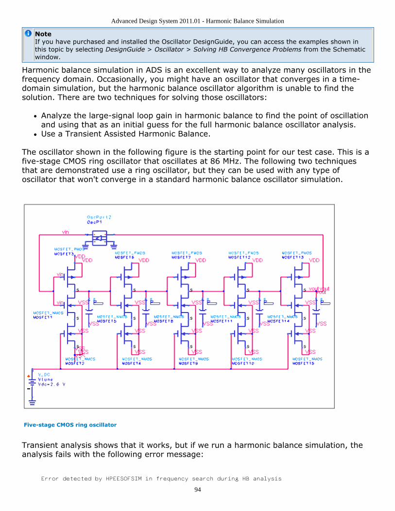
Advanced Design System 2011.01 - Harmonic Balance Simulation
94
NoteIf you have purchased and installed the Oscillator DesignGuide, you can access the examples shown inthis topic by selecting DesignGuide > Oscillator > Solving HB Convergence Problems from the Schematicwindow.
Harmonic balance simulation in ADS is an excellent way to analyze many oscillators in thefrequency domain. Occasionally, you might have an oscillator that converges in a time-domain simulation, but the harmonic balance oscillator algorithm is unable to find thesolution. There are two techniques for solving those oscillators:
Analyze the large-signal loop gain in harmonic balance to find the point of oscillationand using that as an initial guess for the full harmonic balance oscillator analysis.Use a Transient Assisted Harmonic Balance.
The oscillator shown in the following figure is the starting point for our test case. This is afive-stage CMOS ring oscillator that oscillates at 86 MHz. The following two techniquesthat are demonstrated use a ring oscillator, but they can be used with any type ofoscillator that won't converge in a standard harmonic balance oscillator simulation.
Five-stage CMOS ring oscillator
Transient analysis shows that it works, but if we run a harmonic balance simulation, theanalysis fails with the following error message:
Error detected by HPEESOFSIM in frequency search during HB analysis
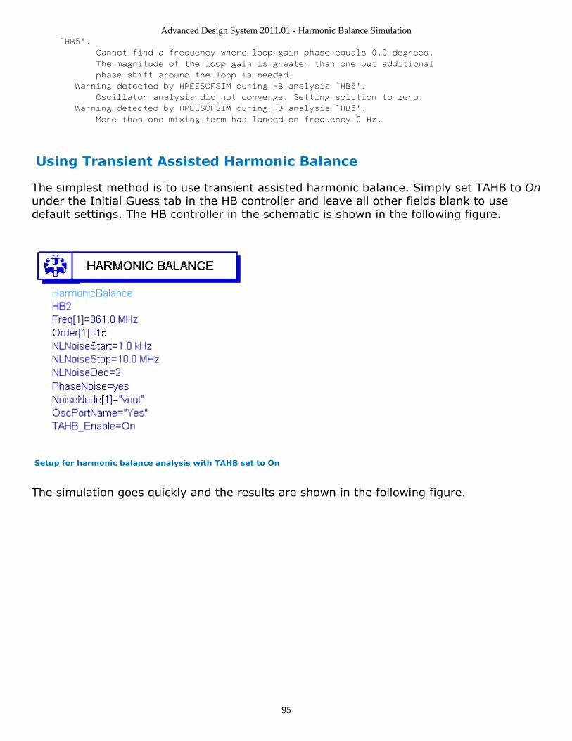
Advanced Design System 2011.01 - Harmonic Balance Simulation
95
`HB5'.
Cannot find a frequency where loop gain phase equals 0.0 degrees.
The magnitude of the loop gain is greater than one but additional
phase shift around the loop is needed.
Warning detected by HPEESOFSIM during HB analysis `HB5'.
Oscillator analysis did not converge. Setting solution to zero.
Warning detected by HPEESOFSIM during HB analysis `HB5'.
More than one mixing term has landed on frequency 0 Hz.
Using Transient Assisted Harmonic Balance
The simplest method is to use transient assisted harmonic balance. Simply set TAHB to Onunder the Initial Guess tab in the HB controller and leave all other fields blank to usedefault settings. The HB controller in the schematic is shown in the following figure.
Setup for harmonic balance analysis with TAHB set to On
The simulation goes quickly and the results are shown in the following figure.
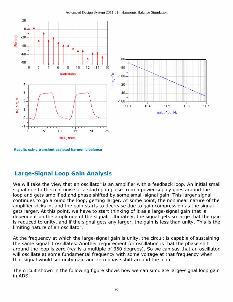
Advanced Design System 2011.01 - Harmonic Balance Simulation
96
Results using transient assisted harmonic balance
Large-Signal Loop Gain Analysis
We will take the view that an oscillator is an amplifier with a feedback loop. An initial smallsignal due to thermal noise or a startup impulse from a power supply goes around theloop and gets amplified and phase shifted by some small-signal gain. This larger signalcontinues to go around the loop, getting larger. At some point, the nonlinear nature of theamplifier kicks in, and the gain starts to decrease due to gain compression as the signalgets larger. At this point, we have to start thinking of it as a large-signal gain that isdependent on the amplitude of the signal. Ultimately, the signal gets so large that the gainis reduced to unity, and if the signal gets any larger, the gain is less than unity. This is thelimiting nature of an oscillator.
At the frequency at which the large-signal gain is unity, the circuit is capable of sustainingthe same signal it oscillates. Another requirement for oscillation is that the phase shiftaround the loop is zero (really a multiple of 360 degrees). So we can say that an oscillatorwill oscillate at some fundamental frequency with some voltage at that frequency whenthat signal would set unity gain and zero phase shift around the loop.
The circuit shown in the following figure shows how we can simulate large-signal loop gainin ADS.
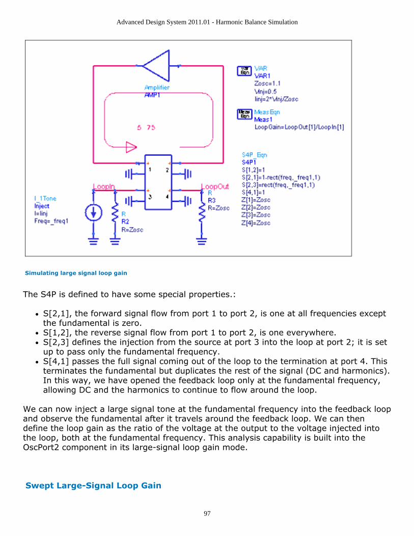
Advanced Design System 2011.01 - Harmonic Balance Simulation
97
Simulating large signal loop gain
The S4P is defined to have some special properties.:
S[2,1], the forward signal flow from port 1 to port 2, is one at all frequencies exceptthe fundamental is zero.S[1,2], the reverse signal flow from port 1 to port 2, is one everywhere.S[2,3] defines the injection from the source at port 3 into the loop at port 2; it is setup to pass only the fundamental frequency.S[4,1] passes the full signal coming out of the loop to the termination at port 4. Thisterminates the fundamental but duplicates the rest of the signal (DC and harmonics).In this way, we have opened the feedback loop only at the fundamental frequency,allowing DC and the harmonics to continue to flow around the loop.
We can now inject a large signal tone at the fundamental frequency into the feedback loopand observe the fundamental after it travels around the feedback loop. We can thendefine the loop gain as the ratio of the voltage at the output to the voltage injected intothe loop, both at the fundamental frequency. This analysis capability is built into theOscPort2 component in its large-signal loop gain mode.
Swept Large-Signal Loop Gain
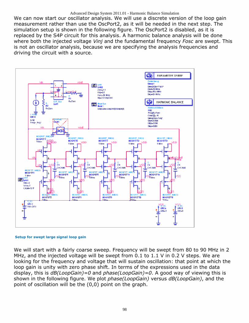
Advanced Design System 2011.01 - Harmonic Balance Simulation
98
We can now start our oscillator analysis. We will use a discrete version of the loop gainmeasurement rather than use the OscPort2, as it will be needed in the next step. Thesimulation setup is shown in the following figure. The OscPort2 is disabled, as it isreplaced by the S4P circuit for this analysis. A harmonic balance analysis will be donewhere both the injected voltage Vinj and the fundamental frequency Fosc are swept. Thisis not an oscillator analysis, because we are specifying the analysis frequencies anddriving the circuit with a source.
Setup for swept large signal loop gain
We will start with a fairly coarse sweep. Frequency will be swept from 80 to 90 MHz in 2MHz, and the injected voltage will be swept from 0.1 to 1.1 V in 0.2 V steps. We arelooking for the frequency and voltage that will sustain oscillation: that point at which theloop gain is unity with zero phase shift. In terms of the expressions used in the datadisplay, this is dB(LoopGain)=0 and phase(LoopGain)=0. A good way of viewing this isshown in the following figure. We plot phase(LoopGain) versus dB(LoopGain), and thepoint of oscillation will be the (0,0) point on the graph.
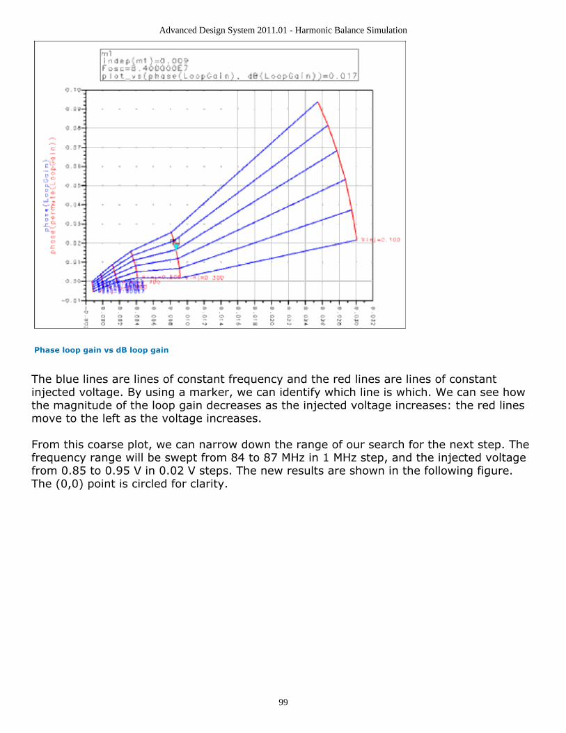
Advanced Design System 2011.01 - Harmonic Balance Simulation
99
Phase loop gain vs dB loop gain
The blue lines are lines of constant frequency and the red lines are lines of constantinjected voltage. By using a marker, we can identify which line is which. We can see howthe magnitude of the loop gain decreases as the injected voltage increases: the red linesmove to the left as the voltage increases.
From this coarse plot, we can narrow down the range of our search for the next step. Thefrequency range will be swept from 84 to 87 MHz in 1 MHz step, and the injected voltagefrom 0.85 to 0.95 V in 0.02 V steps. The new results are shown in the following figure.The (0,0) point is circled for clarity.
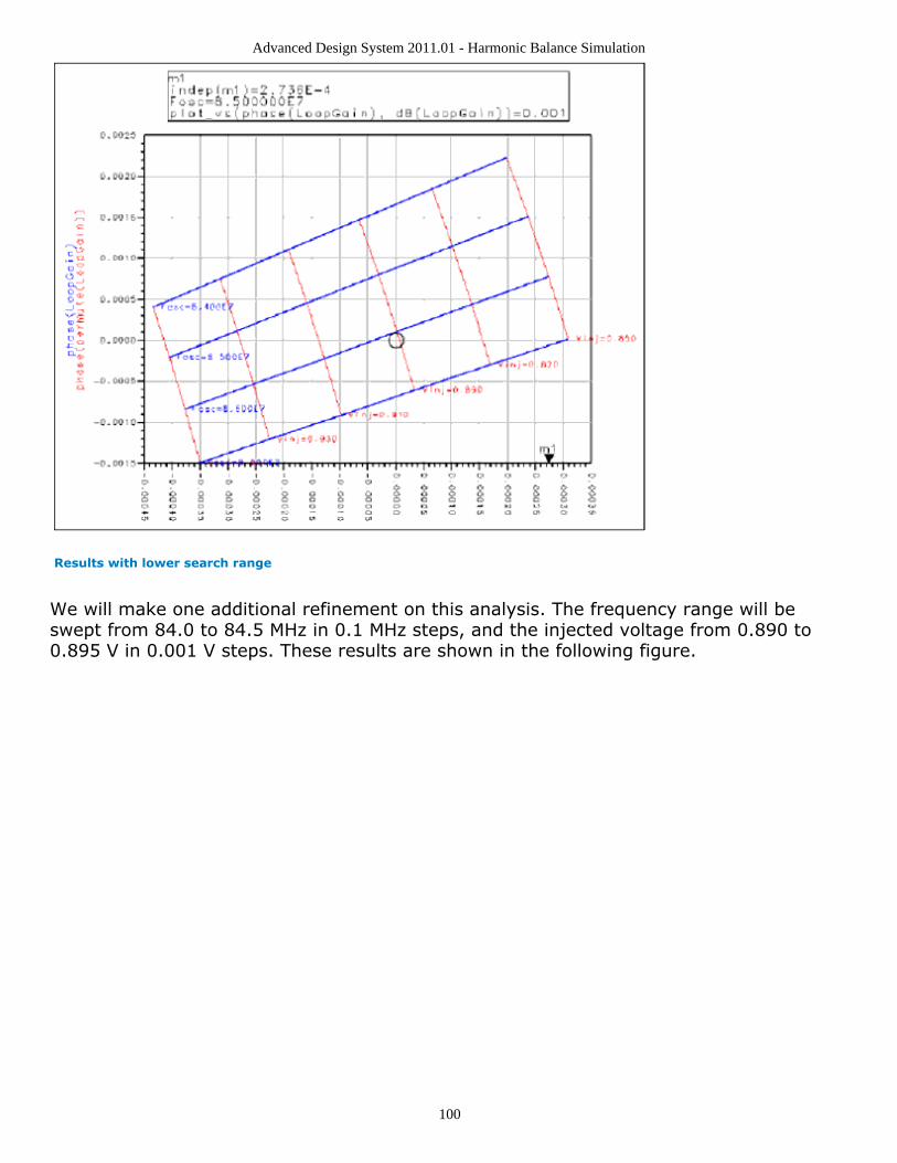
Advanced Design System 2011.01 - Harmonic Balance Simulation
100
Results with lower search range
We will make one additional refinement on this analysis. The frequency range will beswept from 84.0 to 84.5 MHz in 0.1 MHz steps, and the injected voltage from 0.890 to0.895 V in 0.001 V steps. These results are shown in the following figure.
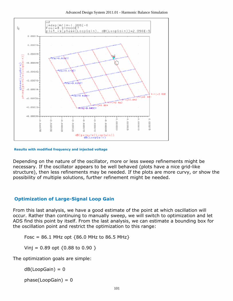
Advanced Design System 2011.01 - Harmonic Balance Simulation
101
Results with modified frequency and injected voltage
Depending on the nature of the oscillator, more or less sweep refinements might benecessary. If the oscillator appears to be well behaved (plots have a nice grid-likestructure), then less refinements may be needed. If the plots are more curvy, or show thepossibility of multiple solutions, further refinement might be needed.
Optimization of Large-Signal Loop Gain
From this last analysis, we have a good estimate of the point at which oscillation willoccur. Rather than continuing to manually sweep, we will switch to optimization and letADS find this point by itself. From the last analysis, we can estimate a bounding box forthe oscillation point and restrict the optimization to this range:
Fosc = 86.1 MHz opt {86.0 MHz to 86.5 MHz}
Vinj = 0.89 opt {0.88 to 0.90 }
The optimization goals are simple:
dB(LoopGain) = 0
phase(LoopGain) = 0
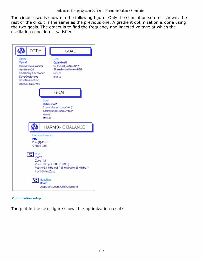
Advanced Design System 2011.01 - Harmonic Balance Simulation
102
The circuit used is shown in the following figure. Only the simulation setup is shown; therest of the circuit is the same as the previous one. A gradient optimization is done usingthe two goals. The object is to find the frequency and injected voltage at which theoscillation condition is satisfied.
Optimization setup
The plot in the next figure shows the optimization results.
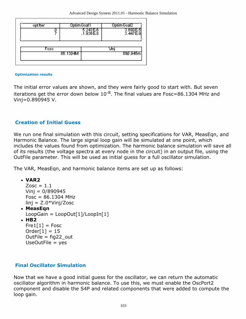
Advanced Design System 2011.01 - Harmonic Balance Simulation
103
Optimization results
The initial error values are shown, and they were fairly good to start with. But seveniterations get the error down below 10-8. The final values are Fosc=86.1304 MHz andVinj=0.890945 V.
Creation of Initial Guess
We run one final simulation with this circuit, setting specifications for VAR, MeasEqn, andHarmonic Balance. The large signal loop gain will be simulated at one point, whichincludes the values found from optimization. The harmonic balance simulation will save allof its results (the voltage spectra at every node in the circuit) in an output file, using theOutFile parameter. This will be used as initial guess for a full oscillator simulation.
The VAR, MeasEqn, and harmonic balance items are set up as follows:
VAR2Zosc = 1.1Vinj = 0/890945Fosc = 86.1304 MHzlinj = Z.0*Vinj/ZoscMeasEqnLoopGain = LoopOut[1]/LoopIn[1]HB2Fre1[1] = FoscOrder[1] = 15OutFile = fig22_outUseOutFile = yes
Final Oscillator Simulation
Now that we have a good initial guess for the oscillator, we can return the automaticoscillator algorithm in harmonic balance. To use this, we must enable the OscPort2component and disable the S4P and related components that were added to compute theloop gain.
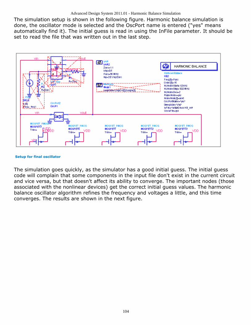
Advanced Design System 2011.01 - Harmonic Balance Simulation
104
The simulation setup is shown in the following figure. Harmonic balance simulation isdone, the oscillator mode is selected and the OscPort name is entered ("yes" meansautomatically find it). The initial guess is read in using the InFile parameter. It should beset to read the file that was written out in the last step.
Setup for final oscillator
The simulation goes quickly, as the simulator has a good initial guess. The initial guesscode will complain that some components in the input file don't exist in the current circuitand vice versa, but that doesn't affect its ability to converge. The important nodes (thoseassociated with the nonlinear devices) get the correct initial guess values. The harmonicbalance oscillator algorithm refines the frequency and voltages a little, and this timeconverges. The results are shown in the next figure.
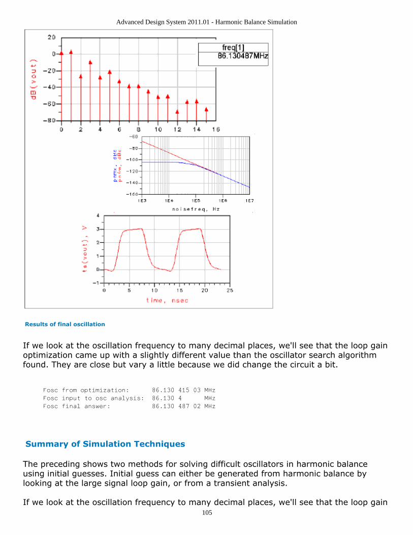
Advanced Design System 2011.01 - Harmonic Balance Simulation
105
Results of final oscillation
If we look at the oscillation frequency to many decimal places, we'll see that the loop gainoptimization came up with a slightly different value than the oscillator search algorithmfound. They are close but vary a little because we did change the circuit a bit.
Fosc from optimization: 86.130 415 03 MHz
Fosc input to osc analysis: 86.130 4 MHz
Fosc final answer: 86.130 487 02 MHz
Summary of Simulation Techniques
The preceding shows two methods for solving difficult oscillators in harmonic balanceusing initial guesses. Initial guess can either be generated from harmonic balance bylooking at the large signal loop gain, or from a transient analysis.
If we look at the oscillation frequency to many decimal places, we'll see that the loop gain
Advanced Design System 2011.01 - Harmonic Balance Simulation
106
optimization came up with a slightly different value than the oscillator search algorithmfound. They are close but vary a little because we did make small changes to the circuit.
Transient method:
Fosc from transient: 86.094 601 MHz
Fosc input to osc analysis: 86.1 MHz
Fosc final answer: 86.131 078 MHz
Loop gain method:
Fosc from optimization: 86.130 415 MHz
Fosc input to osc analysis: 86.130 4 MHz
Fosc final answer: 86.130 487 MHz
The harmonic balance oscillator results from the two methods are very similar. Thefrequencies differ by only 591 Hz, which is a relative difference of 6.9x10⁻⁶.
Advanced Design System 2011.01 - Harmonic Balance Simulation
107
Harmonic Balance for Mixers This topic discusses the use of the Harmonic Balance simulator for standard mixeranalyses and the small signal option in the Harmonic Balance dialog box that simplifiesmixer analyses. It also discusses noise simulations for mixers.
The Small-signal option makes it possible to do a multitone analysis where sidebands areinvolved, as in a mixer analysis. By reducing by 1 the number of large-signal tonesrequired in a conventional harmonic balance analysis, and eliminating the need tocalculate large-signal products, the simulation is computationally efficient.
The sections focusing on setting up noise simulations for mixers describe how tocalculate:
Noise analysis frequency translation of the noiseNonlinear spot noiseNonlinear swept noise
There are two methods of noise simulation. One is to use the parameters on the Noise tabin the harmonic balance dialog box. A second method is to use NoiseCons. UsingNoiseCons, you can set up several noise simulations, thereby eliminating the need tochange the values on the Noise tab in the Harmonic Balance dialog box. With NoiseCons,you can also set parameters to calculate phase noise.
The starting point of this topic assumes you are familiar with the basics of harmonicbalance simulation, as described in Harmonic Balance Basics (cktsimhb).
For details on harmonic balance for mixers and small-signal mixer analysis, see thefollowing topics:
Performing a Basic Mixer Simulation gives the minimum setup for a mixer simulation.Examples of Mixer Simulations gives detailed setups for a variety of mixer analyses,such as looking at output tones, performing a small-signal mixer simulation,calculating conversion gain, and calculating intermodulation distortion.Small-Signal Mode Description is a brief explanation of small-signal mixer simulation.
When you are familiar with basic mixer simulation, see the following topics for details onmixer noise simulation:
Determining Mixer Noise is an example of how to set up a simulation to calculatenoise.Simulating Mixer Noise with NoiseCons illustrates how to perform noise simulationsusing NoiseCon components in ADS.Small-Signal Noise Simulation is an overview of how nonlinear swept noise iscalculated.
Performing a Basic Mixer Simulation
Advanced Design System 2011.01 - Harmonic Balance Simulation
108
For a successful analysis:
By convention, the mixer input port is considered to be port 1, the IF output port isport 2, and the LO input port is port 3. Set up sources and port numbers so that theymatch the mixer convention. You do this by editing the Num field for thesecomponents.Ensure that frequencies are established for all of the frequencies of interest-RF, LO,and IF-in the design.Add the Harmonic Balance simulation component to the schematic and double-clickto edit it. Fill in the fields under the Freq tab:
Enter the RF, LO, and IF as fundamental frequencies and set the order.Assign the LO frequency to Freq[1]; it is easier to achieve convergence if thefrequency of the signal with the largest amplitude is assigned to Freq[1].Since the number of tones in the simulation can affect simulation time, set theMaximum order to limit the number of tones that are considered in thesimulation. For more information, refer to Harmonics and Maximum MixingOrder (cktsimhb).Tone assignment and aliasing error can affect the outcome of a mixersimulation. You may want to select the Params tab and set the FFT Oversampleparameter. For more information refer to Oversampling to Prevent Aliasing(cktsimhb).
For details about other fields, click Help from the dialog box.
Examples of Mixer SimulationsThis section gives detailed setups to perform harmonic balance simulations for:
Finding Mixer Output TonesPerforming a Small-Signal Simulation of a MixerDetermining Mixer Conversion GainDetermining Mixer Intermodulation DistortionDetermining Mixer NoiseSimulating Mixer Noise with NoiseCons
NoteThe Harmonic Balance simulation uses the Harmonic Balance Simulator license (sim_harmonic) which isincluded with all Circuit Design suites except RF Designer. You must have this license to run HarmonicBalance simulations. You can work with examples described here and installed with the software withoutthe license, but you will not be able to simulate them.
Finding Mixer Output Tones
The next figure below illustrates an example setup for determining the amplitudes andrelationships of mixer output tones.
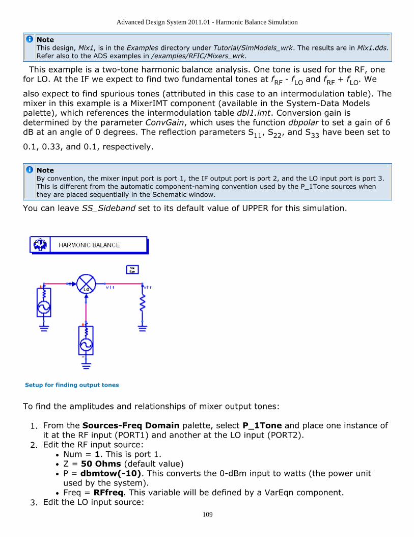
Advanced Design System 2011.01 - Harmonic Balance Simulation
109
NoteThis design, Mix1, is in the Examples directory under Tutorial/SimModels_wrk. The results are in Mix1.dds.Refer also to the ADS examples in /examples/RFIC/Mixers_wrk.
This example is a two-tone harmonic balance analysis. One tone is used for the RF, onefor LO. At the IF we expect to find two fundamental tones at fRF - fLO and fRF + fLO. We
also expect to find spurious tones (attributed in this case to an intermodulation table). Themixer in this example is a MixerIMT component (available in the System-Data Modelspalette), which references the intermodulation table dbl1.imt. Conversion gain isdetermined by the parameter ConvGain, which uses the function dbpolar to set a gain of 6dB at an angle of 0 degrees. The reflection parameters S11, S22, and S33 have been set to
0.1, 0.33, and 0.1, respectively.
NoteBy convention, the mixer input port is port 1, the IF output port is port 2, and the LO input port is port 3.This is different from the automatic component-naming convention used by the P_1Tone sources whenthey are placed sequentially in the Schematic window.
You can leave SS_Sideband set to its default value of UPPER for this simulation.
Setup for finding output tones
To find the amplitudes and relationships of mixer output tones:
From the Sources-Freq Domain palette, select P_1Tone and place one instance of1.it at the RF input (PORT1) and another at the LO input (PORT2).Edit the RF input source:2.
Num = 1. This is port 1.Z = 50 Ohms (default value)P = dbmtow(-10). This converts the 0-dBm input to watts (the power unitused by the system).Freq = RFfreq. This variable will be defined by a VarEqn component.
Edit the LO input source:3.
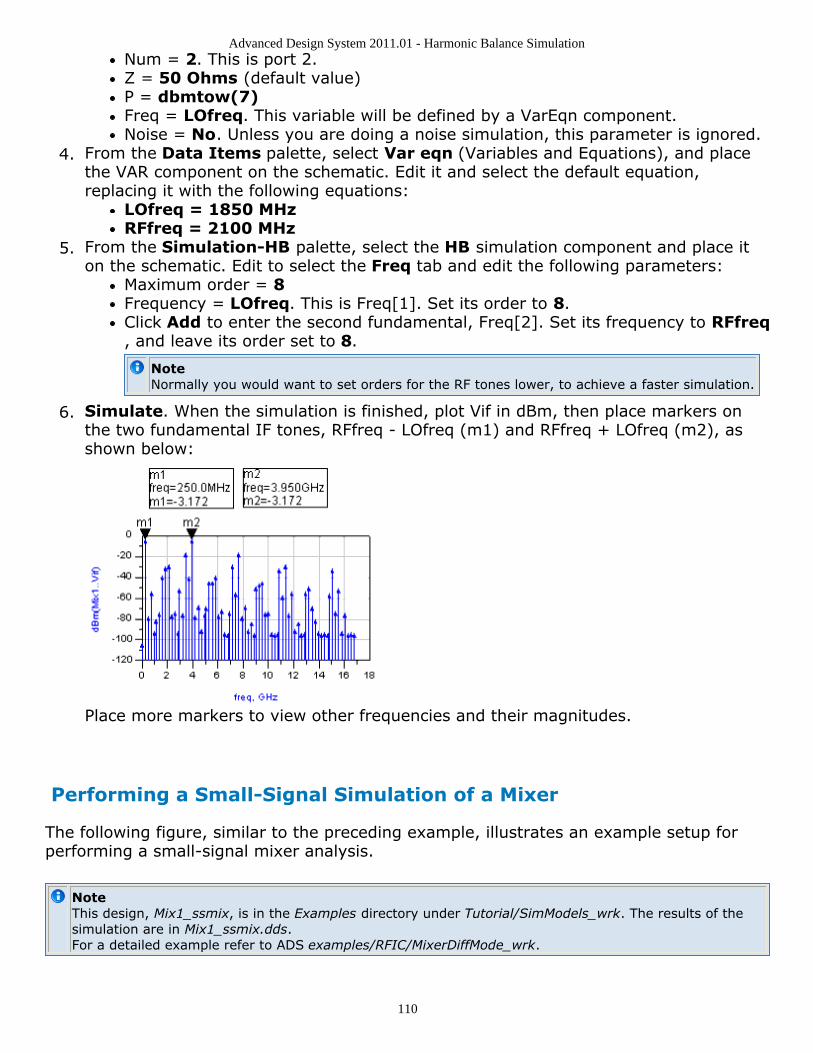
Advanced Design System 2011.01 - Harmonic Balance Simulation
110
Num = 2. This is port 2.Z = 50 Ohms (default value)P = dbmtow(7)Freq = LOfreq. This variable will be defined by a VarEqn component.Noise = No. Unless you are doing a noise simulation, this parameter is ignored.
From the Data Items palette, select Var eqn (Variables and Equations), and place4.the VAR component on the schematic. Edit it and select the default equation,replacing it with the following equations:
LOfreq = 1850 MHzRFfreq = 2100 MHz
From the Simulation-HB palette, select the HB simulation component and place it5.on the schematic. Edit to select the Freq tab and edit the following parameters:
Maximum order = 8Frequency = LOfreq. This is Freq[1]. Set its order to 8.Click Add to enter the second fundamental, Freq[2]. Set its frequency to RFfreq, and leave its order set to 8.
NoteNormally you would want to set orders for the RF tones lower, to achieve a faster simulation.
Simulate. When the simulation is finished, plot Vif in dBm, then place markers on6.the two fundamental IF tones, RFfreq - LOfreq (m1) and RFfreq + LOfreq (m2), asshown below:
Place more markers to view other frequencies and their magnitudes.
Performing a Small-Signal Simulation of a Mixer
The following figure, similar to the preceding example, illustrates an example setup forperforming a small-signal mixer analysis.
NoteThis design, Mix1_ssmix, is in the Examples directory under Tutorial/SimModels_wrk. The results of thesimulation are in Mix1_ssmix.dds.For a detailed example refer to ADS examples/RFIC/MixerDiffMode_wrk.
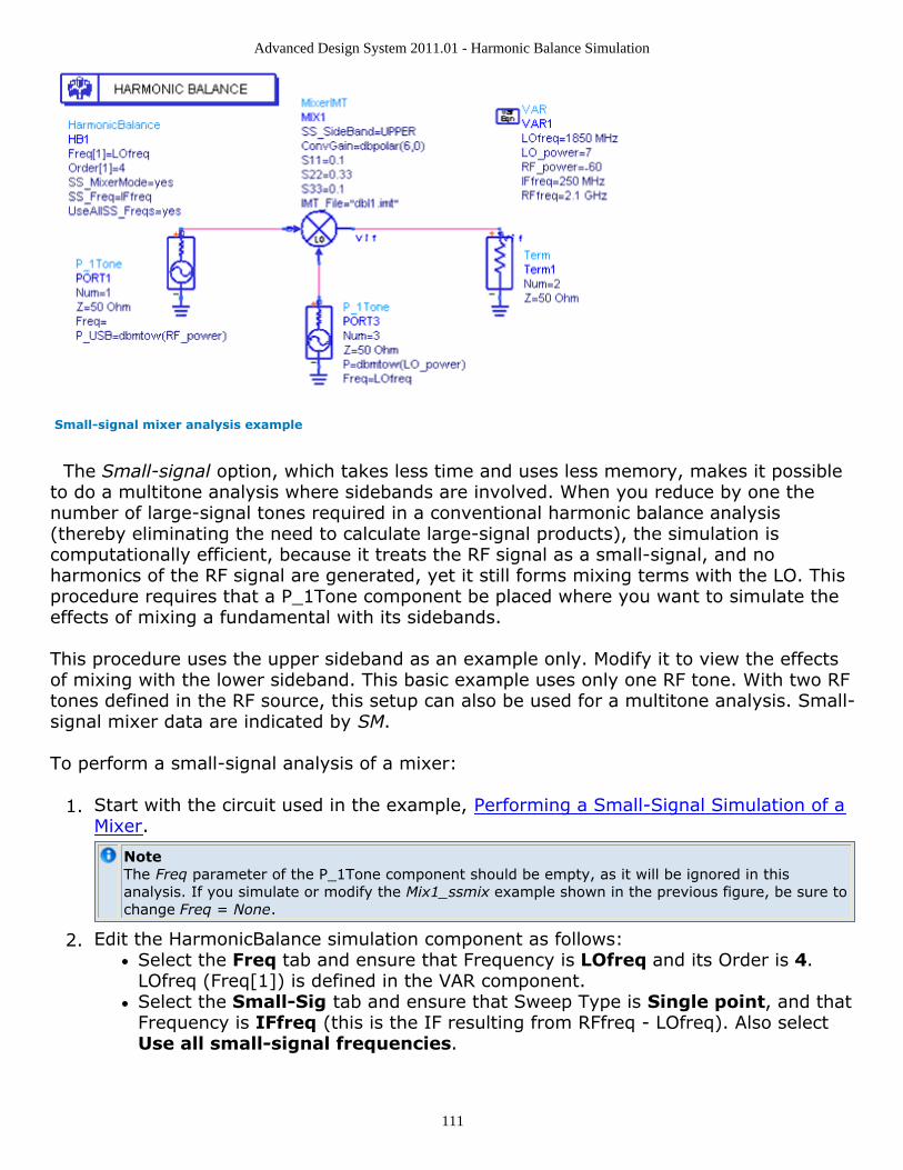
Advanced Design System 2011.01 - Harmonic Balance Simulation
111
Small-signal mixer analysis example
The Small-signal option, which takes less time and uses less memory, makes it possibleto do a multitone analysis where sidebands are involved. When you reduce by one thenumber of large-signal tones required in a conventional harmonic balance analysis(thereby eliminating the need to calculate large-signal products), the simulation iscomputationally efficient, because it treats the RF signal as a small-signal, and noharmonics of the RF signal are generated, yet it still forms mixing terms with the LO. Thisprocedure requires that a P_1Tone component be placed where you want to simulate theeffects of mixing a fundamental with its sidebands.
This procedure uses the upper sideband as an example only. Modify it to view the effectsof mixing with the lower sideband. This basic example uses only one RF tone. With two RFtones defined in the RF source, this setup can also be used for a multitone analysis. Small-signal mixer data are indicated by SM.
To perform a small-signal analysis of a mixer:
Start with the circuit used in the example, Performing a Small-Signal Simulation of a1.Mixer.
NoteThe Freq parameter of the P_1Tone component should be empty, as it will be ignored in thisanalysis. If you simulate or modify the Mix1_ssmix example shown in the previous figure, be sure tochange Freq = None.
Edit the HarmonicBalance simulation component as follows:2.Select the Freq tab and ensure that Frequency is LOfreq and its Order is 4.LOfreq (Freq[1]) is defined in the VAR component.Select the Small-Sig tab and ensure that Sweep Type is Single point, and thatFrequency is IFfreq (this is the IF resulting from RFfreq - LOfreq). Also selectUse all small-signal frequencies.
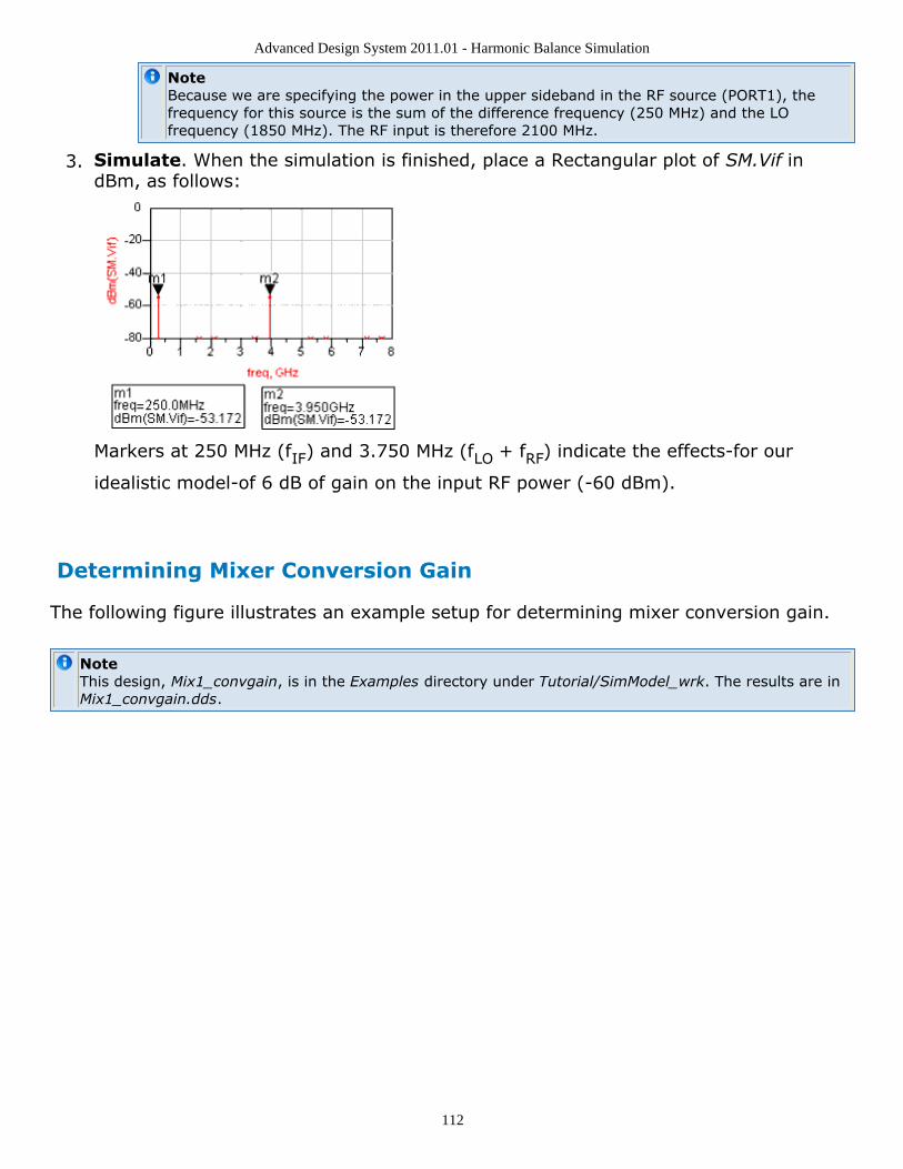
Advanced Design System 2011.01 - Harmonic Balance Simulation
112
NoteBecause we are specifying the power in the upper sideband in the RF source (PORT1), thefrequency for this source is the sum of the difference frequency (250 MHz) and the LOfrequency (1850 MHz). The RF input is therefore 2100 MHz.
Simulate. When the simulation is finished, place a Rectangular plot of SM.Vif in3.dBm, as follows:
Markers at 250 MHz (fIF) and 3.750 MHz (fLO + fRF) indicate the effects-for our
idealistic model-of 6 dB of gain on the input RF power (-60 dBm).
Determining Mixer Conversion Gain
The following figure illustrates an example setup for determining mixer conversion gain.
NoteThis design, Mix1_convgain, is in the Examples directory under Tutorial/SimModel_wrk. The results are inMix1_convgain.dds.

Advanced Design System 2011.01 - Harmonic Balance Simulation
113
Example determining mixer conversion gain
This example uses the basic Mixer component from the System-Amps & Mixers palette,and also illustrates the use of the Krylov method. While a small-signal mixer analysis canbe used to determine conversion gain, the method described here, in which the RF signalis not assumed to be small, should be used if the RF signal is large enough to drive themixer into compression.
To determine mixer conversion gain:
Start with the circuit in the example, Finding Mixer Output Tones.1.Edit the P_1Tone component at the RF source (PORT1)s:2.
P= dbmtow(Power_RF). Power_RF will be established by an equation.Freq = RFfreq
Edit the P_1Tone component at the LO source (PORT2):3.P= dbmtow(0)Freq = LOfreq
Using the VAR component, enter the following equations (note the use of the4.underscore before dBm):RF_power = -30 _dBmLO_power = -10 _dBmLOfreq = 1850 MHzIFfreq = RFfreq - LOfreqRFfreq = 2100 MHz
NoteIn ADS, dBm is not a recognized unit. The underscore in front of dBm (as in _dBm ) allows this unitto be used for documentation purposes without causing the simulator to issue a warning.
Edit the Harmonic Balance Simulation component, select the Freq tab, and edit the5.following parameters:
Maximum order = 5
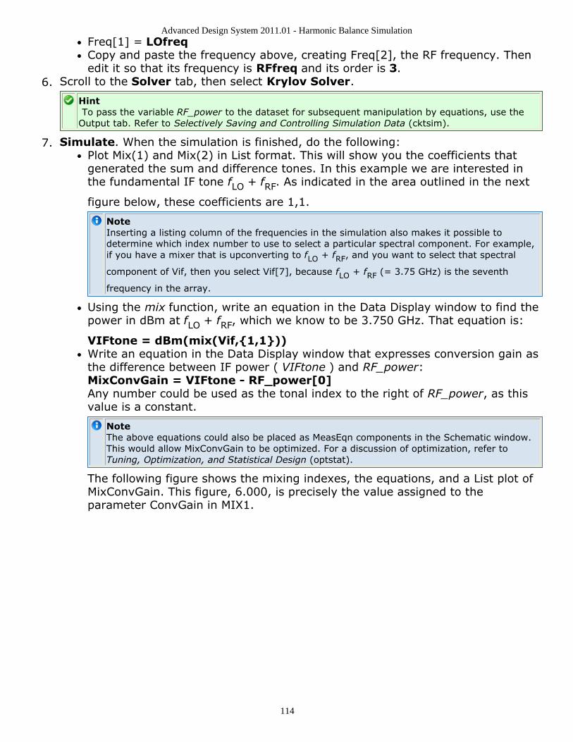
Advanced Design System 2011.01 - Harmonic Balance Simulation
114
Freq[1] = LOfreqCopy and paste the frequency above, creating Freq[2], the RF frequency. Thenedit it so that its frequency is RFfreq and its order is 3.
Scroll to the Solver tab, then select Krylov Solver.6.
Hint To pass the variable RF_power to the dataset for subsequent manipulation by equations, use theOutput tab. Refer to Selectively Saving and Controlling Simulation Data (cktsim).
Simulate. When the simulation is finished, do the following:7.Plot Mix(1) and Mix(2) in List format. This will show you the coefficients thatgenerated the sum and difference tones. In this example we are interested inthe fundamental IF tone fLO + fRF. As indicated in the area outlined in the next
figure below, these coefficients are 1,1.
NoteInserting a listing column of the frequencies in the simulation also makes it possible todetermine which index number to use to select a particular spectral component. For example,if you have a mixer that is upconverting to fLO + fRF, and you want to select that spectral
component of Vif, then you select Vif[7], because fLO + fRF (= 3.75 GHz) is the seventh
frequency in the array.
Using the mix function, write an equation in the Data Display window to find thepower in dBm at fLO + fRF, which we know to be 3.750 GHz. That equation is:
VIFtone = dBm(mix(Vif,{1,1}))Write an equation in the Data Display window that expresses conversion gain asthe difference between IF power ( VIFtone ) and RF_power:MixConvGain = VIFtone - RF_power[0]Any number could be used as the tonal index to the right of RF_power, as thisvalue is a constant.
NoteThe above equations could also be placed as MeasEqn components in the Schematic window.This would allow MixConvGain to be optimized. For a discussion of optimization, refer toTuning, Optimization, and Statistical Design (optstat).
The following figure shows the mixing indexes, the equations, and a List plot ofMixConvGain. This figure, 6.000, is precisely the value assigned to theparameter ConvGain in MIX1.
Advanced Design System 2011.01 - Harmonic Balance Simulation
115
Mixer conversion gain indexes, equations, and plot
Determining Mixer Intermodulation Distortion
The following figure illustrates an example for determining mixer intermodulationdistortion (IMD). The approach used here is commonly referred to as third-order intercept(TOI) analysis.
NoteThis design, Mix2_TOI, is in the Examples directory under Tutorial/SimModels_wrk. The results are inMix2_TOI.dds.
This example is similar to Performing a Small-Signal Simulation of a Mixer, except that itinvolves three tones as well as equations that determine Freq[2] and Freq[3].
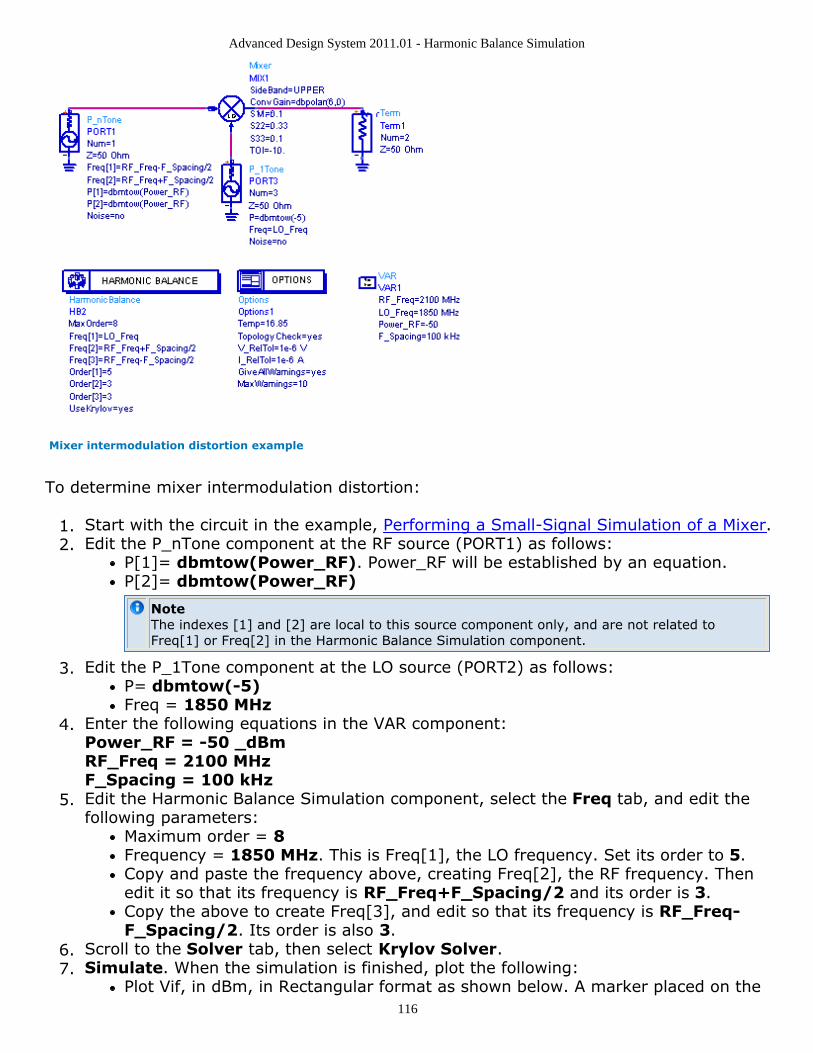
Advanced Design System 2011.01 - Harmonic Balance Simulation
116
Mixer intermodulation distortion example
To determine mixer intermodulation distortion:
Start with the circuit in the example, Performing a Small-Signal Simulation of a Mixer.1.Edit the P_nTone component at the RF source (PORT1) as follows:2.
P[1]= dbmtow(Power_RF). Power_RF will be established by an equation.P[2]= dbmtow(Power_RF)
NoteThe indexes [1] and [2] are local to this source component only, and are not related toFreq[1] or Freq[2] in the Harmonic Balance Simulation component.
Edit the P_1Tone component at the LO source (PORT2) as follows:3.P= dbmtow(-5)Freq = 1850 MHz
Enter the following equations in the VAR component:4.Power_RF = -50 _dBmRF_Freq = 2100 MHzF_Spacing = 100 kHzEdit the Harmonic Balance Simulation component, select the Freq tab, and edit the5.following parameters:
Maximum order = 8Frequency = 1850 MHz. This is Freq[1], the LO frequency. Set its order to 5.Copy and paste the frequency above, creating Freq[2], the RF frequency. Thenedit it so that its frequency is RF_Freq+F_Spacing/2 and its order is 3.Copy the above to create Freq[3], and edit so that its frequency is RF_Freq-F_Spacing/2. Its order is also 3.
Scroll to the Solver tab, then select Krylov Solver.6.Simulate. When the simulation is finished, plot the following:7.
Plot Vif, in dBm, in Rectangular format as shown below. A marker placed on the
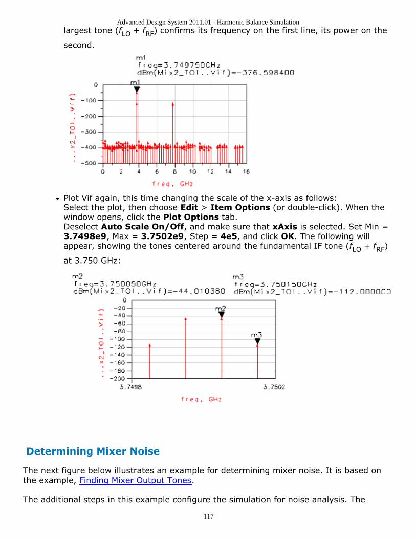
Advanced Design System 2011.01 - Harmonic Balance Simulation
117
largest tone (fLO + fRF) confirms its frequency on the first line, its power on the
second.
Plot Vif again, this time changing the scale of the x-axis as follows:Select the plot, then choose Edit > Item Options (or double-click). When thewindow opens, click the Plot Options tab.Deselect Auto Scale On/Off, and make sure that xAxis is selected. Set Min =3.7498e9, Max = 3.7502e9, Step = 4e5, and click OK. The following willappear, showing the tones centered around the fundamental IF tone (fLO + fRF)
at 3.750 GHz:
Determining Mixer Noise
The next figure below illustrates an example for determining mixer noise. It is based onthe example, Finding Mixer Output Tones.
The additional steps in this example configure the simulation for noise analysis. The
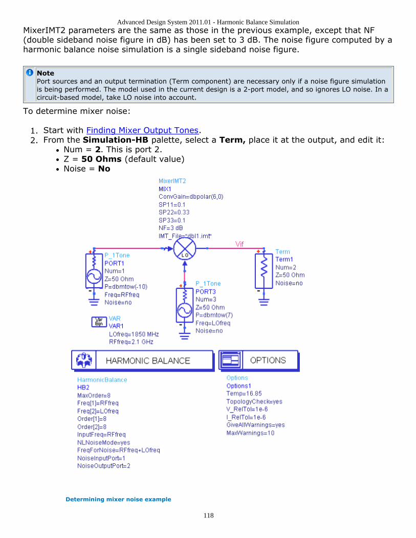
Advanced Design System 2011.01 - Harmonic Balance Simulation
118
MixerIMT2 parameters are the same as those in the previous example, except that NF(double sideband noise figure in dB) has been set to 3 dB. The noise figure computed by aharmonic balance noise simulation is a single sideband noise figure.
NotePort sources and an output termination (Term component) are necessary only if a noise figure simulationis being performed. The model used in the current design is a 2-port model, and so ignores LO noise. In acircuit-based model, take LO noise into account.
To determine mixer noise:
Start with Finding Mixer Output Tones.1.From the Simulation-HB palette, select a Term, place it at the output, and edit it:2.
Num = 2. This is port 2.Z = 50 Ohms (default value)Noise = No
Determining mixer noise example
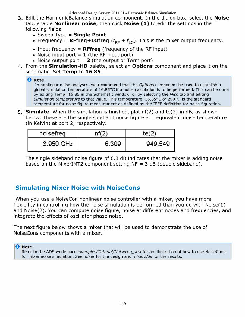
Advanced Design System 2011.01 - Harmonic Balance Simulation
119
Edit the HarmonicBalance simulation component. In the dialog box, select the Noise3.tab, enable Nonlinear noise, then click Noise (1) to edit the settings in thefollowing fields:
Sweep Type = Single PointFrequency = RFfreq+LOfreq (fRF + fLO). This is the mixer output frequency.
Input frequency = RFfreq (frequency of the RF input)Noise input port = 1 (the RF input port)Noise output port = 2 (the output or Term port)
From the Simulation-HB palette, select an Options component and place it on the4.schematic. Set Temp to 16.85.
Note In nonlinear noise analyses, we recommend that the Options component be used to establish aglobal simulation temperature of 16.85°C if a noise calculation is to be performed. This can be doneby editing Temp=16.85 in the Schematic window, or by selecting the Misc tab and editingSimulation temperature to that value. This temperature, 16.85°C or 290 K, is the standardtemperature for noise figure measurement as defined by the IEEE definition for noise figuration.
Simulate. When the simulation is finished, plot nf(2) and te(2) in dB, as shown5.below. These are the single sideband noise figure and equivalent noise temperature(in Kelvin) at port 2, respectively.
The single sideband noise figure of 6.3 dB indicates that the mixer is adding noisebased on the MixerIMT2 component setting NF = 3 dB (double sideband).
Simulating Mixer Noise with NoiseCons
When you use a NoiseCon nonlinear noise controller with a mixer, you have moreflexibility in controlling how the noise simulation is performed than you do with Noise(1)and Noise(2). You can compute noise figure, noise at different nodes and frequencies, andintegrate the effects of oscillator phase noise.
The next figure below shows a mixer that will be used to demonstrate the use ofNoiseCons components with a mixer.
NoteRefer to the ADS workspace examples/Tutorial/Noisecon_wrk for an illustration of how to use NoiseConsfor mixer noise simulation. See mixer for the design and mixer.dds for the results.
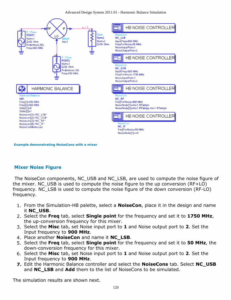
Advanced Design System 2011.01 - Harmonic Balance Simulation
120
Example demonstrating NoiseCons with a mixer
Mixer Noise Figure
The NoiseCon components, NC_USB and NC_LSB, are used to compute the noise figure ofthe mixer. NC_USB is used to compute the noise figure to the up conversion (RF+LO)frequency. NC_LSB is used to compute the noise figure of the down conversion (RF-LO)frequency.
From the Simulation-HB palette, select a NoiseCon, place it in the design and name1.it NC_USB.Select the Freq tab, select Single point for the frequency and set it to 1750 MHz,2.the up-conversion frequency for this mixer.Select the Misc tab, set Noise input port to 1 and Noise output port to 2. Set the3.Input frequency to 900 MHz.Place another NoiseCon and name it NC_LSB.4.Select the Freq tab, select Single point for the frequency and set it to 50 MHz, the5.down-conversion frequency for this mixer.Select the Misc tab, set Noise input port to 1 and Noise output port to 2. Set the6.Input frequency to 900 MHz.Edit the Harmonic Balance controller and select the NoiseCons tab. Select NC_USB7.and NC_LSB and Add them to the list of NoiseCons to be simulated.
The simulation results are shown next.
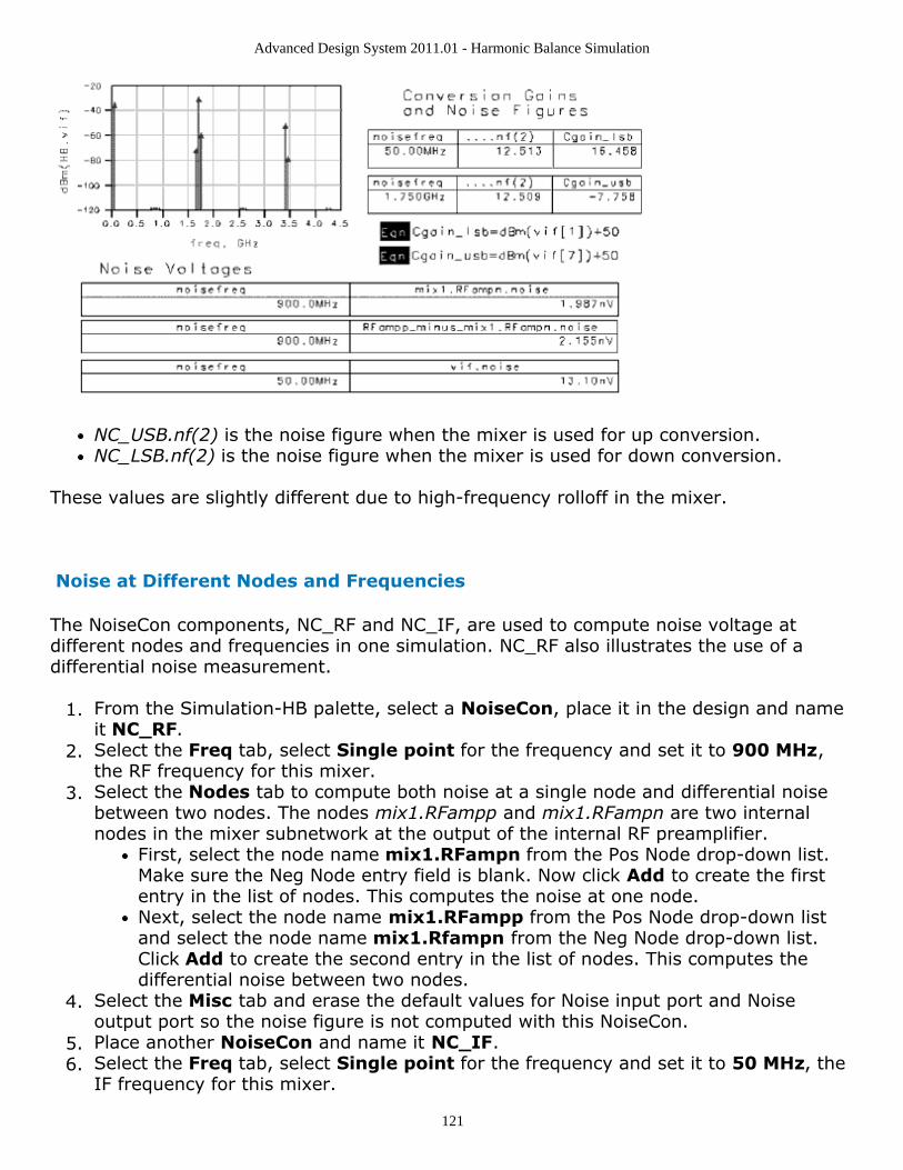
Advanced Design System 2011.01 - Harmonic Balance Simulation
121
NC_USB.nf(2) is the noise figure when the mixer is used for up conversion.NC_LSB.nf(2) is the noise figure when the mixer is used for down conversion.
These values are slightly different due to high-frequency rolloff in the mixer.
Noise at Different Nodes and Frequencies
The NoiseCon components, NC_RF and NC_IF, are used to compute noise voltage atdifferent nodes and frequencies in one simulation. NC_RF also illustrates the use of adifferential noise measurement.
From the Simulation-HB palette, select a NoiseCon, place it in the design and name1.it NC_RF.Select the Freq tab, select Single point for the frequency and set it to 900 MHz,2.the RF frequency for this mixer.Select the Nodes tab to compute both noise at a single node and differential noise3.between two nodes. The nodes mix1.RFampp and mix1.RFampn are two internalnodes in the mixer subnetwork at the output of the internal RF preamplifier.
First, select the node name mix1.RFampn from the Pos Node drop-down list.Make sure the Neg Node entry field is blank. Now click Add to create the firstentry in the list of nodes. This computes the noise at one node.Next, select the node name mix1.RFampp from the Pos Node drop-down listand select the node name mix1.Rfampn from the Neg Node drop-down list.Click Add to create the second entry in the list of nodes. This computes thedifferential noise between two nodes.
Select the Misc tab and erase the default values for Noise input port and Noise4.output port so the noise figure is not computed with this NoiseCon.Place another NoiseCon and name it NC_IF.5.Select the Freq tab, select Single point for the frequency and set it to 50 MHz, the6.IF frequency for this mixer.
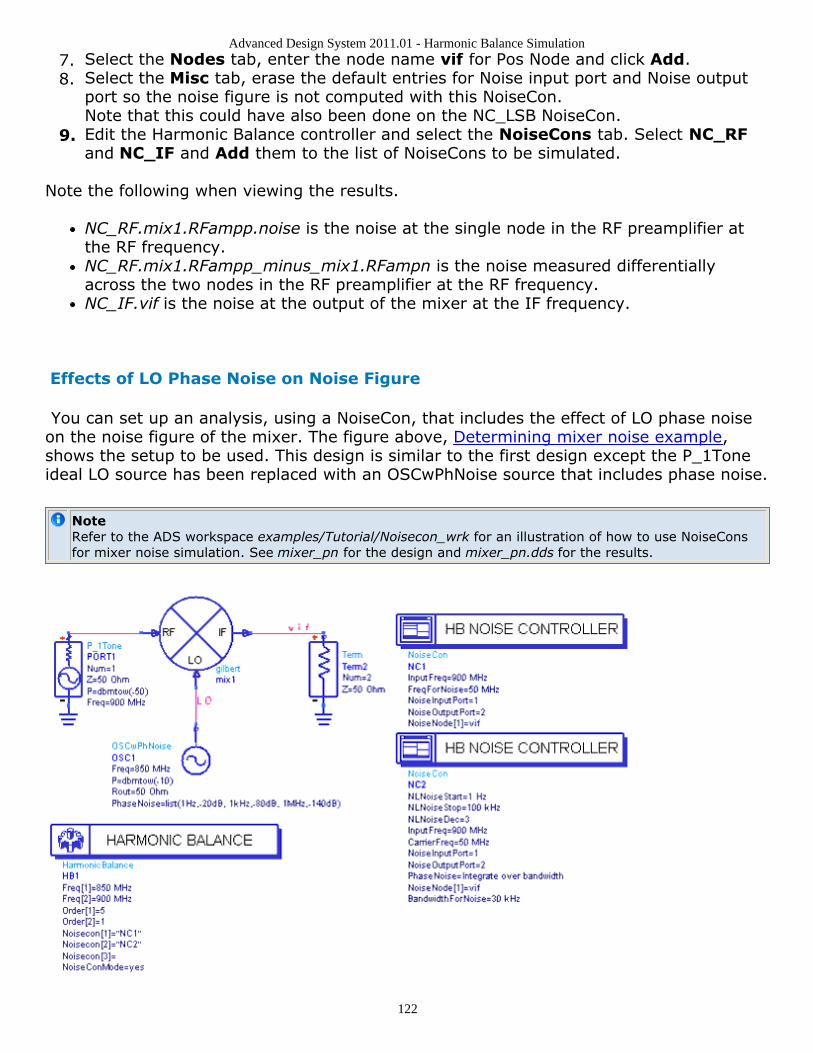
Advanced Design System 2011.01 - Harmonic Balance Simulation
122
Select the Nodes tab, enter the node name vif for Pos Node and click Add.7.Select the Misc tab, erase the default entries for Noise input port and Noise output8.port so the noise figure is not computed with this NoiseCon.Note that this could have also been done on the NC_LSB NoiseCon.Edit the Harmonic Balance controller and select the NoiseCons tab. Select NC_RF9.and NC_IF and Add them to the list of NoiseCons to be simulated.
Note the following when viewing the results.
NC_RF.mix1.RFampp.noise is the noise at the single node in the RF preamplifier atthe RF frequency.NC_RF.mix1.RFampp_minus_mix1.RFampn is the noise measured differentiallyacross the two nodes in the RF preamplifier at the RF frequency.NC_IF.vif is the noise at the output of the mixer at the IF frequency.
Effects of LO Phase Noise on Noise Figure
You can set up an analysis, using a NoiseCon, that includes the effect of LO phase noiseon the noise figure of the mixer. The figure above, Determining mixer noise example,shows the setup to be used. This design is similar to the first design except the P_1Toneideal LO source has been replaced with an OSCwPhNoise source that includes phase noise.
NoteRefer to the ADS workspace examples/Tutorial/Noisecon_wrk for an illustration of how to use NoiseConsfor mixer noise simulation. See mixer_pn for the design and mixer_pn.dds for the results.
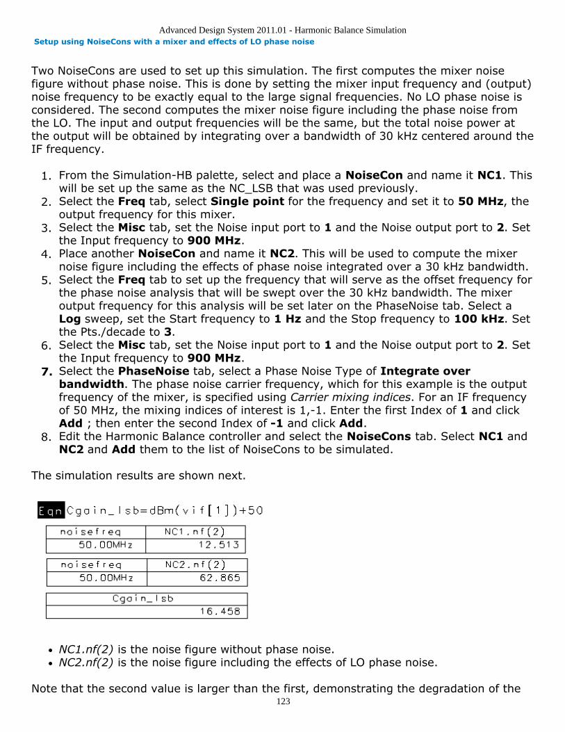
Advanced Design System 2011.01 - Harmonic Balance Simulation
123
Setup using NoiseCons with a mixer and effects of LO phase noise
Two NoiseCons are used to set up this simulation. The first computes the mixer noisefigure without phase noise. This is done by setting the mixer input frequency and (output)noise frequency to be exactly equal to the large signal frequencies. No LO phase noise isconsidered. The second computes the mixer noise figure including the phase noise fromthe LO. The input and output frequencies will be the same, but the total noise power atthe output will be obtained by integrating over a bandwidth of 30 kHz centered around theIF frequency.
From the Simulation-HB palette, select and place a NoiseCon and name it NC1. This1.will be set up the same as the NC_LSB that was used previously.Select the Freq tab, select Single point for the frequency and set it to 50 MHz, the2.output frequency for this mixer.Select the Misc tab, set the Noise input port to 1 and the Noise output port to 2. Set3.the Input frequency to 900 MHz.Place another NoiseCon and name it NC2. This will be used to compute the mixer4.noise figure including the effects of phase noise integrated over a 30 kHz bandwidth.Select the Freq tab to set up the frequency that will serve as the offset frequency for5.the phase noise analysis that will be swept over the 30 kHz bandwidth. The mixeroutput frequency for this analysis will be set later on the PhaseNoise tab. Select aLog sweep, set the Start frequency to 1 Hz and the Stop frequency to 100 kHz. Setthe Pts./decade to 3.Select the Misc tab, set the Noise input port to 1 and the Noise output port to 2. Set6.the Input frequency to 900 MHz.Select the PhaseNoise tab, select a Phase Noise Type of Integrate over7.bandwidth. The phase noise carrier frequency, which for this example is the outputfrequency of the mixer, is specified using Carrier mixing indices. For an IF frequencyof 50 MHz, the mixing indices of interest is 1,-1. Enter the first Index of 1 and clickAdd ; then enter the second Index of -1 and click Add.Edit the Harmonic Balance controller and select the NoiseCons tab. Select NC1 and8.NC2 and Add them to the list of NoiseCons to be simulated.
The simulation results are shown next.
NC1.nf(2) is the noise figure without phase noise.NC2.nf(2) is the noise figure including the effects of LO phase noise.
Note that the second value is larger than the first, demonstrating the degradation of the
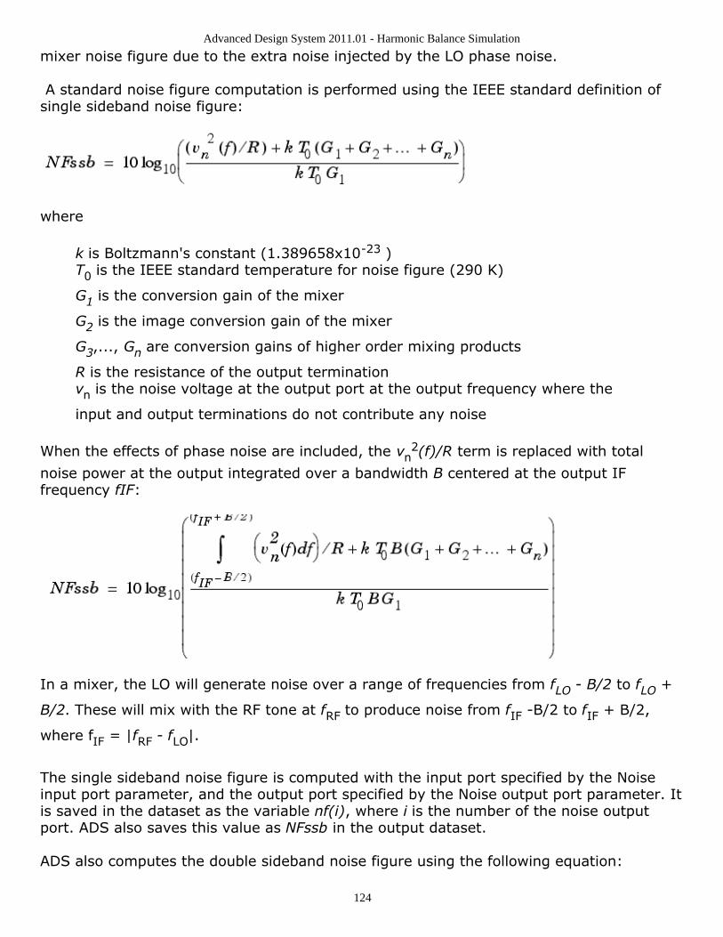
Advanced Design System 2011.01 - Harmonic Balance Simulation
124
mixer noise figure due to the extra noise injected by the LO phase noise.
A standard noise figure computation is performed using the IEEE standard definition ofsingle sideband noise figure:
where
k is Boltzmann's constant (1.389658x10⁻²³ )T0 is the IEEE standard temperature for noise figure (290 K)
G1 is the conversion gain of the mixer
G2 is the image conversion gain of the mixer
G3,..., Gn are conversion gains of higher order mixing products
R is the resistance of the output terminationvn is the noise voltage at the output port at the output frequency where the
input and output terminations do not contribute any noise
When the effects of phase noise are included, the vn2(f)/R term is replaced with total
noise power at the output integrated over a bandwidth B centered at the output IFfrequency fIF:
In a mixer, the LO will generate noise over a range of frequencies from fLO - B/2 to fLO +
B/2. These will mix with the RF tone at fRF to produce noise from fIF -B/2 to fIF + B/2,
where fIF = |fRF - fLO|.
The single sideband noise figure is computed with the input port specified by the Noiseinput port parameter, and the output port specified by the Noise output port parameter. Itis saved in the dataset as the variable nf(i), where i is the number of the noise outputport. ADS also saves this value as NFssb in the output dataset.
ADS also computes the double sideband noise figure using the following equation:
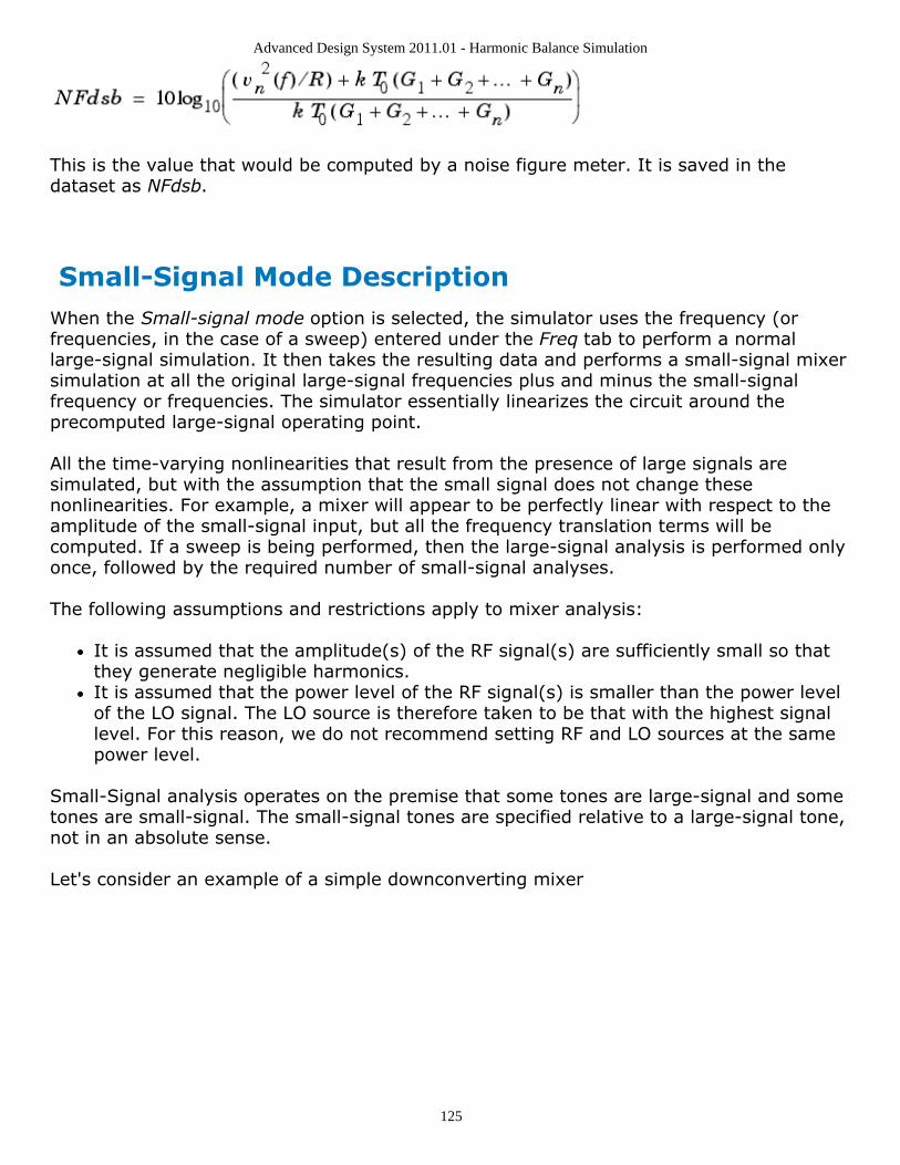
Advanced Design System 2011.01 - Harmonic Balance Simulation
125
This is the value that would be computed by a noise figure meter. It is saved in thedataset as NFdsb.
Small-Signal Mode DescriptionWhen the Small-signal mode option is selected, the simulator uses the frequency (orfrequencies, in the case of a sweep) entered under the Freq tab to perform a normallarge-signal simulation. It then takes the resulting data and performs a small-signal mixersimulation at all the original large-signal frequencies plus and minus the small-signalfrequency or frequencies. The simulator essentially linearizes the circuit around theprecomputed large-signal operating point.
All the time-varying nonlinearities that result from the presence of large signals aresimulated, but with the assumption that the small signal does not change thesenonlinearities. For example, a mixer will appear to be perfectly linear with respect to theamplitude of the small-signal input, but all the frequency translation terms will becomputed. If a sweep is being performed, then the large-signal analysis is performed onlyonce, followed by the required number of small-signal analyses.
The following assumptions and restrictions apply to mixer analysis:
It is assumed that the amplitude(s) of the RF signal(s) are sufficiently small so thatthey generate negligible harmonics.It is assumed that the power level of the RF signal(s) is smaller than the power levelof the LO signal. The LO source is therefore taken to be that with the highest signallevel. For this reason, we do not recommend setting RF and LO sources at the samepower level.
Small-Signal analysis operates on the premise that some tones are large-signal and sometones are small-signal. The small-signal tones are specified relative to a large-signal tone,not in an absolute sense.
Let's consider an example of a simple downconverting mixer
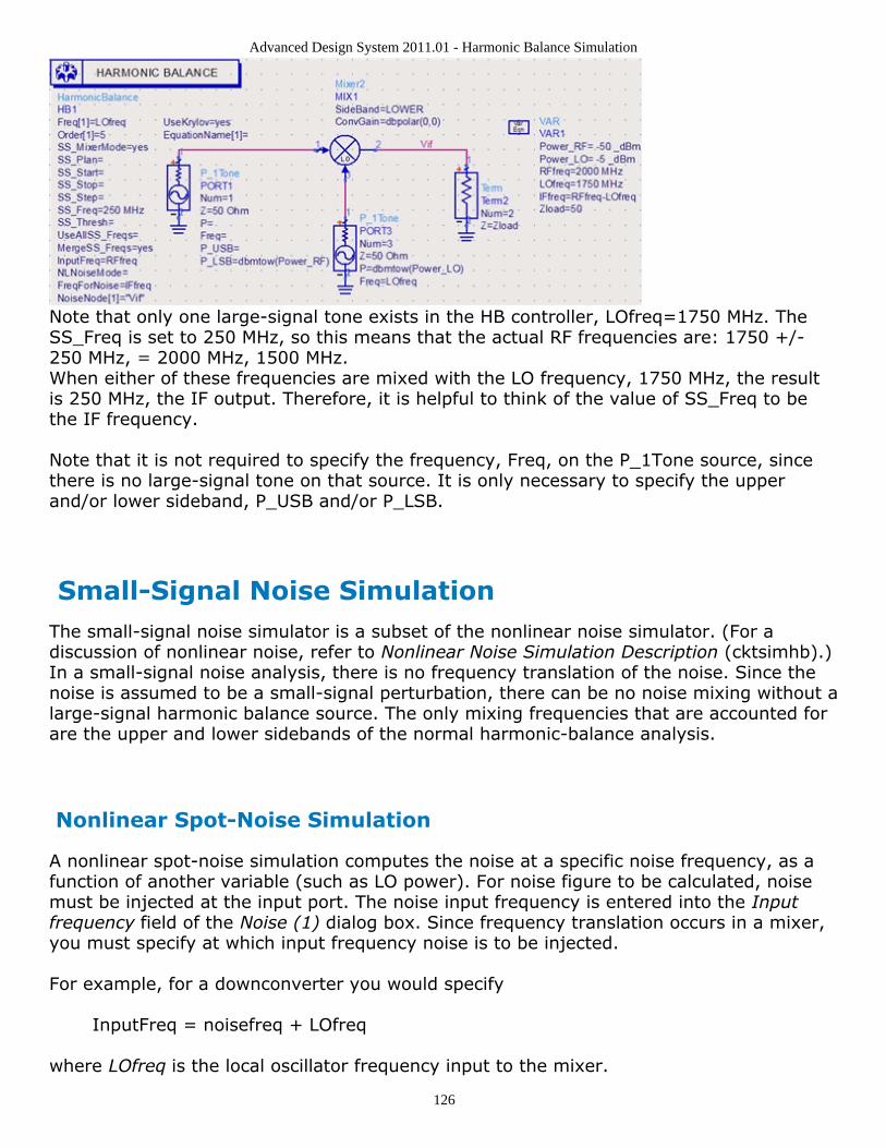
Advanced Design System 2011.01 - Harmonic Balance Simulation
126
Note that only one large-signal tone exists in the HB controller, LOfreq=1750 MHz. TheSS_Freq is set to 250 MHz, so this means that the actual RF frequencies are: 1750 +/-250 MHz, = 2000 MHz, 1500 MHz.When either of these frequencies are mixed with the LO frequency, 1750 MHz, the resultis 250 MHz, the IF output. Therefore, it is helpful to think of the value of SS_Freq to bethe IF frequency.
Note that it is not required to specify the frequency, Freq, on the P_1Tone source, sincethere is no large-signal tone on that source. It is only necessary to specify the upperand/or lower sideband, P_USB and/or P_LSB.
Small-Signal Noise Simulation The small-signal noise simulator is a subset of the nonlinear noise simulator. (For adiscussion of nonlinear noise, refer to Nonlinear Noise Simulation Description (cktsimhb).)In a small-signal noise analysis, there is no frequency translation of the noise. Since thenoise is assumed to be a small-signal perturbation, there can be no noise mixing without alarge-signal harmonic balance source. The only mixing frequencies that are accounted forare the upper and lower sidebands of the normal harmonic-balance analysis.
Nonlinear Spot-Noise Simulation
A nonlinear spot-noise simulation computes the noise at a specific noise frequency, as afunction of another variable (such as LO power). For noise figure to be calculated, noisemust be injected at the input port. The noise input frequency is entered into the Inputfrequency field of the Noise (1) dialog box. Since frequency translation occurs in a mixer,you must specify at which input frequency noise is to be injected.
For example, for a downconverter you would specify
InputFreq = noisefreq + LOfreq
where LOfreq is the local oscillator frequency input to the mixer.
Advanced Design System 2011.01 - Harmonic Balance Simulation
127
The downconverter will shift INPUTFREQ to
InputFreq - LOfreq = (noisefreq + LOfreq) - LOfreq = noisefreq
For an upconverter, INPUTFREQ would be
InputFreq = noisefreq - LOfreq
Single-Frequency Nonlinear Spot Noise
The simulation results of a single-point analysis have no independent variable andtherefore cannot be plotted on a rectangular plot, however, the data can be displayed in alisting column. Note that noise voltages are always rms.
If the amplitude of the RF signal is small compared to that of the LO, then the noise mixedby the LO and its harmonics will dominate, and simulations can be run much more quicklyby simply including the LO and its harmonics in the harmonic balance noise analysis.
Multiple-Frequency Nonlinear Spot Noise
A sweep can also be used to compute noise at the specified noise frequency as a functionof a variable. If an independent variable is in the nonlinear noise data, the data can beplotted on a rectangular plot.
Swept-Noise Simulation
A nonlinear swept-noise simulation computes the noise at a swept list of noisefrequencies with another optional swept variable (for example, LO power). The result isanalogous to a spectrum analyzer display. Nonlinear swept-noise analysis differs fromnonlinear spot-noise analysis in that the noise frequency (in the Noise frequency area inthe Noise (1) dialog box) is allowed to be swept in a manner similar to the way aspectrum analyzer sweeps a noise floor.
The noise frequency can be an expression if the noise frequency is swept. For example, tocompute the noise figure of an upper sideband mixer in which the noise output frequencyis swept but the LO frequency is fixed, set the parameter Input frequency as follows:
InputFreq = noisefreq + LOfreq
where noisefreq is the noise frequency and LOfreq is an equation defining the fixed LOfrequency.
The results of the analysis can be plotted on a rectangular plot. The independent variable

Advanced Design System 2011.01 - Harmonic Balance Simulation
128
of the swept nonlinear noise analysis is always noisefreq.
Advanced Design System 2011.01 - Harmonic Balance Simulation
129
Transient Assisted Harmonic Balance This topic describes the automated transient assisted harmonic balance simulation(TAHB). For a harmonic balance simulation, an initial guess of the solution is needed. Forcircuits that are highly nonlinear and contain sharp-edged waveforms (such as dividers), atransient simulation often provides a good initial guess for the starting point of harmonicbalance. In a TAHB simulation, a transient is performed to generate the initial guess forthe harmonic balance. Then an HB simulation is performed using the transient initialguess. The simulator automatically generates the transient initial guess when the Enablecheck box is selected.
It is strongly recommended to use this simulation technique for divider circuits and otherswith sharp edged or pulse-like waveforms. We suggest that you use the TAHB Auto mode,which is the default setting, for optimal performance. The simulator will turn on TAHBautomatically if the circuit involves a divider. The user can choose the TAHB On mode ifthe circuit does not involve a divider, yet sharp edged or pulse-like waveforms areexpected.
If you are not familiar with the harmonic balance simulator, see Harmonic Balance Basics(cktsimhb).
The following topics describe details about automated transient assisted harmonicbalance:
Setting Additional Transient Parameters describes how to set parameters forautomated TAHB.Using a One-Tone Transient for a Multi-Tone Harmonic Balance describes how toinstruct the transient simulator to perform a one-tone simulation.Using Sweeps and Optimization Simulations describes how to use sweeps andoptimization simulations with automated TAHB.Outputting the Transient Data to the Dataset describes how to control transient dataoutput to the dataset.
For details about each individual TAHB parameter, see Setting Up the Initial Guess(cktsimhb).
Setting Additional Transient ParametersThe transient simulator uses intelligent defaults and determines a steady state solution forthe initial guess in harmonic balance. For the automated TAHB, you are not required to setany transient parameters. However, you may set the transient parameters by choosingthe TAHB On mode if desired.
The first parameter to set is StopTime. The default for StopTime is 100 cycles of thecommensurate frequency. In a single tone analysis, this is simply the value of Freq [1].This parameter determines how long transient should run when generating the initialguess. If the transient simulator detects steady state before it reaches the StopTime, then
Advanced Design System 2011.01 - Harmonic Balance Simulation
130
it will end at that point (earlier than the StopTime ), then proceed with the harmonicbalance simulation. When the transient does not find a steady state solution, thenHarmonic Balance uses the last transient data point as an initial guess.
The next parameter to set is MaxTimeStep. The default for MaxTimeStep is1/(2*2*Maximum Frequency). In a single tone transient analysis, the maximum frequencyis Freq[1]*Order[1]. Adjust this parameter if a smaller or larger time step is required.
The simulator displays the values that it determined for StopTime and MaxTimeStep in thestatus window.
The parameter Min Detect Steady State Time sets the earliest point in time that thetransient simulator starts checking for steady state conditions. The default is two periodsof the fundamental frequency for autonomous circuits, and 10 periods of the fundamentalfrequency for non-autonomous circuits such as an oscillator. The units for this parameterare in seconds. If your circuit exhibits a large amount of over/undershoot, then this needsto be larger than the default so that the detector will begin to check for steady state aftersome of the initial transients have settled.
The parameter IV_RelTol is the transient current and voltage relative tolerance. Thedefault value is 1e-3. This is a relative tolerance for transient only. If relative tolerancesare set (on Options controller) and the IV_RelTol is given, then it will override the relativetolerances for the Simulator Option's relative tolerances for the transient simulation only.This parameter simply allows for having two sets of relative tolerances, one for transientand the other for harmonic balance.
The Transient Other parameter makes it possible to set transient parameters that are notfound in the TAHB tab. For example, you can set the following transient convolutionparameter ImpMaxFreq =10 GHz using the Transient Other parameter. To see all of thetransient parameters, please see the Transient/Convolution Simulation documentation.
When TAHB_Enable is set to Auto, a user-supplied initial guess will be honored and TAHBwill be turned off by the simulator. When TAHB is set to On, you will not be able to supplyan initial guess file. For more information, please see Transient Assisted Harmonic Balance- TAHB (adshbapp) in the Guide to Harmonic Balance Simulation in ADS (adshbapp).
Using a One-Tone Transient for a Multi-ToneHarmonic Balance The Use only Freq[1] for transient parameter instructs the transient simulator to performa one-tone simulation, and to use only the value of Freq[1] parameter set for theHarmonic Balance simulation for determining the StopTime and MaxTimeStep. Thisparameter is enabled by default. If there are multiple frequencies set for the HBsimulation and this parameter is enabled, then sources in the circuit at the otherfrequencies will be turned off for the transient portion only. It is recommended to performa one-tone transient simulation for a multi-tone HB simulation. Also, Freq[1] should be setto the frequency of the most nonlinear tone.
Advanced Design System 2011.01 - Harmonic Balance Simulation
131
Using Sweeps and Optimization Simulations Statistical simulations such as optimization, yield, Monte Carlo, DOE, and yield-optimization are not supported with automated TAHB. The simulation will terminateprematurely if such simulation types have TAHB set to On. If TAHB is set to Auto, thesimulator will proceed without using TAHB.
Swept simulations are supported with automated TAHB. In ADS, there are two ways tosweep a parameter - using the Sweep tab on the Harmonic Balance controller or using theParameter Sweep controller. When sweeping a parameter on the Sweep tab, a transientsimulation is done for the harmonic balance simulation of the first sweep point only. Whensweeping a parameter on the Parameter Sweep controller, a transient simulation is donefor the first sweep point only, unless the Restart parameter is enabled on the HarmonicBalance controller's Initial Guess tab. When Restart is enabled, a transient simulation isdone at each sweep point which generates a new transient initial guess for each sweeppoint of the harmonic balance simulation.
Outputting the Transient Data to the Dataset The data from the transient simulation can be output to the dataset by enabling theOutput transient data to dataset parameter. By default, this parameter is disabled and thetransient simulation results are not in the dataset. Recall that the transient was used onlyto generate the initial guess for harmonic balance. If the transient results are desired inthe dataset, then be sure to enable this parameter by checking the box. Proceed withcaution for very large circuits since the dataset can grow to be very large if both transientand harmonic balance results are included.
Advanced Design System 2011.01 - Harmonic Balance Simulation
132
Harmonic Balance Assisted HarmonicBalance This topic describes the automated harmonic balance assisted harmonic balancesimulation (HBAHB). Using this method when performing a multi-tone harmonic balancesimulation allows the simulator to decide automatically which tones to use in generatingthe final HB solution. For example, instead of simulating a three-tone circuit directly, it ispossible to simulate a one-tone, then use the result as an initial guess for a two-tone, andfinally use that result as an initial guess for the third tone. HBAHB is both fast and robust,particularly for large multi-tone simulations of mixer circuits to determine gain and IP3.
HBAHB applies only to multi-tone simulations. By default, this feature is enabled withinthe HB simulator. The simulator determines the optimal sequence of tones to simulate.Depending upon various conditions, the simulator may decide to simulate a three-tone HBsimulation with only the first tone, then use that result as an initial guess directly for athree-tone.
If you are not familiar with the harmonic balance simulator, see Harmonic Balance Basics(cktsimhb).
The following topics describe details about automated HBAHB:
Modes of HBAHB OperationHBAHB, Parameter Sweeps, and NoiseHBAHB and TAHBHBAHB and Non-Convergence
Modes of HBAHB Operation There are three modes for the HBAHB - Auto, On, and Off. The default mode is Auto.
To set the HBAHB mode:
Place the HB controller on the schematic and open its setup dialog box.1.On the Initial Guess tab, in the HBAHB section, select the mode.2.
In the Auto mode, the simulator decides whether or not to perform the HBAHB,and the optimal sequence of tones to simulate.In the On mode, the HBAHB always performs a simulation at each tone.In the Off mode, the HBAHB is not performed at all. When the HBAHB is off, astandard multi-tone HB simulation is performed.
For additional setup information, see Setting Up the Initial Guess (cktsimhb).
When selecting Solver parameters for a harmonic balance simulation with the HBAHB setto Auto, it is recommended that you set Convergence Mode to Auto and Solver Type toAuto (see Selecting a Harmonic Balance Solver Technique (cktsimhb)). These settings
Advanced Design System 2011.01 - Harmonic Balance Simulation
133
ensure that simulation of the intermediate tones is both fast and robust, and that theoptimal solver is selected when simulating the different tones.
HBAHB, Parameter Sweeps, and Noise When performing a swept simulation, HBAHB occurs only for the first, or innermost,sweep point. When simulating a noise analyses, the HBAHB occurs prior to the noise. Thismeans that the noise analyses is not performed at the intermediate tones.
HBAHB and TAHB HBAHB will not be performed if TAHB takes place. The HB analysis will read in thetransient solution as the initial guess.
If you provide an initial guess using Initial Guess parameters InFile and UseInFile, HBAHBwill not be performed so long as the supplied initial guess file exists. If the file does notexist, the simulator will decide whether or not to perform HBAHB. Details about settingparameters for Initial Guess, HBAHB, and TAHB are located in Setting Up the Initial Guess(cktsimhb).
HBAHB and Non-Convergence At any point of time during the HBAHB analysis, if non-convergence occurs, thesimulation will stop HBAHB and resort to a standard multi-tone HB analyses. A new DCinitial guess will also be recomputed. If TAHB was enabled, then the transient initial guesswill be restored.


![ECE1254 – MODELING OF MULTIPHYSICS SYSTEMS 1 The Harmonic Balance … · 2014. 4. 9. · harmonic balance method [1], thus in this project only this version will be considered.](https://static.documents.pub/doc/80x56/60b62e485844d81b4366b4f3/ece1254-a-modeling-of-multiphysics-systems-1-the-harmonic-balance-2014-4-9.jpg)


![Nonlinear device characterization using harmonic load pull ......generate various harmonic frequencies apart from the fundamental frequency. Harmonic Balance (HB), [Nakhla, 1976][Rizzoli,](https://static.documents.pub/doc/80x56/5f0f56657e708231d443a94f/nonlinear-device-characterization-using-harmonic-load-pull-generate-various.jpg)

