HEAT KERNEL ANALYSIS AND CAMERON-MARTINSUBGROUP FOR INFINITE DIMENSIONAL GROUPS

MARIA GORDINADepartment of Mathematics and Statistics,

McMaster University,Hamilton, ON L8S 4K1

Canada

Abstract. The heat kernel measure µt is constructed on GL(H), the groupof invertible operators on a complex Hilbert space H. This measure is deter-mined by an infinite dimensional Lie algebra g and a Hermitian inner producton it. The Cameron-Martin subgroup GCM is defined and its properties arediscussed. In particular, there is an isometry from the L2

µt-closure of holomor-

phic polynomials into a space Ht(GCM ) of functions holomorphic on GCM .This means that any element from this L2

µt-closure of holomorphic polynomi-

als has a version holomorphic on GCM . In addition, there is an isometry fromHt(GCM ) into a Hilbert space associated with the tensor algebra over g. Thelatter isometry is an infinite dimensional analog of the Taylor expansion. Asexamples we discuss a complex orthogonal group and a complex symplecticgroup.

Table of Contents

1. Introduction 22. Notation and main results 23. Estimates of derivatives of holomorphic functions 54. Isometries 75. The heat kernel measure 106. Approximation of the process 167. Cameron-Martin subgroup 198. Holomorphic polynomials and skeletons 249. Examples 28References 31

Key words and phrases. Heat kernel measure, holomorphic function, infinite dimensionalgroup, infinite dimensional Lie algebra, stochastic differential equation.

1

2 MARIA GORDINA

1. Introduction

Our goal is to study Hilbert spaces of holomorphic functions on a group asso-ciated with an infinite dimensional Lie algebra g which is itself equipped with aHermitian inner product (·, ·) and corresponding norm | · |. We assume that g is aLie subalgebra of B(H), the space of bounded linear operators on a complex sepa-rable Hilbert space H. The group under consideration is a Lie subgroup of GL(H),the group of invertible elements of B(H). Note that B(H) is the natural (infinitedimensional) Lie algebra of GL(H) with the commutator as a Lie bracket.

One of the main ingredients in this work is the construction of the heat kernelmeasure on GL(H) which is determined by g and the norm | · |. In some casesit is possible to show that the heat kernel measure is supported in a subgroup ofGL(H) (see Section 9). The construction of the heat kernel measure requires theuse of stochastic differential equations in a Hilbert space. We will assume that g isa subspace of the Hilbert-Schmidt operators on H.

It is well known that the Cameron-Martin subspace plays an important role foran abstract Wiener space. Analogously, we define the Cameron-Martin subgroup,GCM , and discuss its properties. One of these properties is that functions in the L2-closure of holomorphic polynomials have holomorphic versions on GCM . Following[15, 16] we call these versions skeletons. The map taking an L2-function to itsskeleton is an isometry to Ht(GCM ), a space of functions holomorphic on GCM

with a direct limit-type norm derived from finite dimensional approximations toGCM . We also show that the Taylor map, from holomorphic functions on GCM

into a dual of the universal enveloping algebra of g, is isometric on Ht(GCM ). Thisisomtery is a noncommutative version of one of the isomorphisms between differentrepresentations of a bosonic Fock space.

An outline of the history of the subject has been given in [7, 8]. We shouldmention here works by Sugita [15, 16] for an abstract complex Wiener space, inparticular, his results on skeletons of L2-functions on the Cameron-Martin subspace.

Acknowledgement. I thank Professor B. Driver, Professor L. Gross and Pro-fessor B. Hall for their help throughout the process of preparation of this work.

2. Notation and main results

To describe results of this paper in more detail we need to use finite dimensionalapproximations to g. Let G1 ⊆ G2 ⊆ ... ⊆ Gn ⊆ ... ⊆ B(H) be a sequenceof complex connected (finite dimensional) Lie subgroups of GL(H). We assumethat their Lie algebras gn ⊆ B(H) are equipped with consistent Hermitian innerproducts, that is, (·, ·)n+m|gn = (·, ·)n, where (·, ·)n is the inner product on gn. Thecorresponding norm is denoted by | · |n.

Let g =∞⋃

n=1gn with the Hermitian inner product (ξ, η) = (ξ, η)n for any ξ, η ∈ gn.

We assume that |x| > ‖x‖ for any x ∈ g, where ‖ · ‖ is the operator norm. Denoteby g∞ the closure of g in the norm | · |, that is, all elements of finite norm. Wealso assume that the closure coincides with the completion of g with respect to thenorm | · |. Note that g∞ is a subset of B(H).

Let d denote the Riemannian metric d(y, z) = infh1∫

0

∣

∣

∣h−1h∣

∣

∣ ds, where h :

[0, 1] → GL(H) is a piecewise differentiable path, h(0) = y, h(1) = z, h = dhds ,

ANALYSIS ON INFINITE DIMENSIONAL GROUPS 3

h′ = h−1h ∈ g∞. Let G∞ be the closure of∞⋃

n=1Gn in the Riemannian metric

d∞ = infn dn, where dn is the Riemannian metric on Gn. Again we assume thatthe closure coincides with the completion. By Ht(G∞) we denote a space of holo-morphic functions on G∞ with a certain direct limit-type norm ‖·‖t,∞. The precisedefinition is given in Section 4.

Let (1 −D)−1X f =

∑∞k=0(D

kf)(X) be the series of all derivatives of a functionf on G∞. Then the Taylor map (1 − D)−1

I is an isometry from Ht(G∞) into asubspace, J0

t , of the dual of the tensor algebra of g∞ equipped with the norm

|α|2t =∞∑

k=0

tk

k!|αk|2, α =

∞∑

k=0

αk, αk ∈ (g⊗k)∗, k = 0, 1, 2, ..., t > 0

See Notation 3.2 and Notation 4.2 for more detailed definitions. The followingtheorem will be proved in Section 4.Theorem. Ht(G∞) is a Hilbert space and (1−D)−1

I is an isometry from Ht(G∞)into J0

t .Moreover, in case the Gn are simply connected Theorem 4.5 gives the image

of (1 − D)−1I , which can be informally described as a completion of the universal

enveloping algebra.The heat kernel measure is constructed in Section 5 using stochastic differential

equations on Hilbert spaces, in this case on the space of Hilbert-Schmidt operators.Denote by HS the space of Hilbert-Schmidt operators on H with the Hilbert-Schmidt (Hermitian) inner product (·, ·)HS and corresponding real inner product〈·, ·〉HS = Re(·, ·)HS . In most of the results of this paper we assume that Gn ⊂I +HS, gn ⊂ HS. The following is a summary of results contained in Theorem 5.1and Theorem 5.4Theorem. Let Wt be the Wiener process in HS with covariance determined bythe norm on g∞. Then the stochastic differential equation

dXt = XtdWt,

X0 = I

has a unique solution in (I + HS) ∩GL(H).The transition probability of the process Xt determines the fundamental solution

of the heat equation with the following informal Laplacian

(∆v)(X) =12

∞∑

n=1

(ξnξnv)(X),

where ξn∞n=1 is an orthonormal basis of g∞ as a real space with the real innerproduct 〈ξ, η〉 = Re(ξ, η) and (ξnv)(X) = d

dt |t=0 v(Xetξn) for a function v :I + HS → R. The corresponding measure is called the heat kernel measure andthe space of functions square integrable with respect to this measure is denoted byL2(I + HS, µt) and the norm by ‖ · ‖t.

In addition to G∞ we consider the Cameron-Martin subgroup.

Definition 2.1. GCM = x ∈ B(H) : d(x, I) < ∞ is called the Cameron-Martinsubgroup.

Proposition 7.1 proves that GCM is a group. Note that G∞ ⊂ GCM and thefollowing theorem shows that under a condition on the Lie bracket they are actuallyequal. The next theorem will be proved in Section 7.

4 MARIA GORDINA

Theorem. If |[x, y]| 6 C |x| |y| for all x, y ∈ g∞, then1. GCM = G∞.2. The exponential map is a diffeomorphism from a neighborhood of 0 onto aneighborhood of I in GCM .

Note that under the condition of this theorem g∞ is a Lie algebra.Naturally defined holomorphic polynomials on I + HS play an important role

in several results. One of them is that there is a natural isometry from the spaceof holomorphic polynomials HP to Ht(G∞). To prove this we use approximationsto the process Yt + I discussed in Section 6. In addition, this isometry definesholomorphic skeletons on GCM for the elements of the closure of HP in L2(I +HS, µt). This closure is denoted by HL2(I + HS, µt). The following results arecontained in Theorem 8.7 and Theorem 8.5.Theorem.1. HP ⊂ L2(I + HS, µt).2. The identity ‖f‖t,∞ = ‖f‖t for any f ∈ HP extends to an isometry IG∞ fromHL2(I + HS, µt) into Ht(G∞).

3. Suppose pnL2(I+HS,µt)−−−−−−−−→

n→∞f, pn ∈ HP. Then there is a holomorphic function f ,

a skeleton of f , on GCM such that pn(x) → f(x) for any x ∈ GCM .We will denote the skeleton map by IGCM . Note that elements of HL2(I +

HS, µt) are defined up to a set of µt-measure zero. Still the map IGCM gives aholomorphic version on GCM of any element from HL2(I + HS, µt), even thoughGCM itself might be of µt-measure zero. In addition, IGCM f |G∞ is actually theisometry IG∞ from part 2 of the last theorem. This means that for holomorphicpolynomials the skeleton map is the restriction map (to GCM ).

Finally, Section 9 provides several examples to this abstract setting. One ofthe examples is the Hilbert-Schmidt complex orthogonal group which has beendiscussed in [7]. In addition we consider the Hilbert-Schmidt complex symplecticgroup and a group of infinite diagonal matrices.

For some g and natural norms | · | on it, the Taylor map is an isometry betweentrivial spaces (see Section 9). But we show that for the natural condition on thenorm | · | considered in this paper, there are non-constant functions in Ht(G∞).Namely, this space contains all holomorphic polynomials. Indeed, Theorem 8.7proves that the holomorphic polynomials are square integrable with respect to theheat kernel measure. Then in the same theorem we show that the L2-norm of apolynomial is equal to the Ht(G∞)-norm.

The following commutative diagram illustrates all the isometries described inthis paper:

HL2(I + HS, µt)

skeleton mapIGCM

IG∞

@@

@@R

- -Ht(GCM ) Ht(G∞) J0t

restriction map Taylor map

ANALYSIS ON INFINITE DIMENSIONAL GROUPS 5

3. Estimates of derivatives of holomorphic functions

Let µnt be the heat kernel measure on Gn; let HL2(Gn, µn

t ) be the space ofholomorphic functions square integrable with respect to µn

t .

Notation 3.1. ‖f‖L2(Gn,µnt ) = ‖f‖t,n.

Notation 3.2. Suppose f is a function from GCM to C. Let (Df)(X) denote theunique element of g∗∞ (as a complex space) such that

(Df)(X)(ξ) = (ξf)(X) =ddt

∣

∣

∣

∣

t=0f(Xetξ), ξ ∈ g∞, X ∈ G∞(GCM ),

if the derivative exists. Similarly (Dkf)(X) denotes the unique element of (g⊗k∞ )∗

such that

(Dkf)(X)(β) = (βf)(X), β ∈ g⊗k∞ , X ∈ GCM

and (Dknf)(X) denotes a unique element of (g∗n)⊗k = (g⊗k

n )∗ such that

(Dknf)(X)(β) = (βf)(X), β ∈ g⊗k

n , X ∈ Gn.

We will use the following notation:

(1−D)−1X f =

∞∑

k=0

(Dkf)(X) and (1−Dn)−1X f =

∞∑

k=0

(Dknf)(X).

The following estimate was proved by Driver and Gross in [5] for f ∈ HL2(Gn, µnt ):

|(βf)(g)|2(g⊗kn )

∗ 6 ‖f‖2t,nk!|β|2n

rk e|g|2n/s, for g ∈ Gn, r > 0, s + r 6 t, β ∈ g⊗k

n ,

where |(βf)(g)|(g⊗kn )

∗ is ((TgGn)∗)⊗k-norm (which can be identified with (g∗n)⊗k)and |g|n = dn(I, g). We will need a slight modification of this estimate. Takingsupremum over all β ∈ g⊗k

n , |β|n = 1, we get

|(Dknf)(g)|2(g∗n)⊗k 6 ‖f‖2t,n

k!rk e|g|

2n/s,(3.1)

where Dkn is defined for Gn and gn by Notation 3.2. Note that if ‖f‖t,n are uniformly

bounded, then (3.1) gives a uniform bound, i.e. a bound independent of n. Thefollowing estimates can be proved for Dk

n:

Lemma 3.3. Let r > 0, q + r 6 t,X, Y ∈ Gn, f ∈ HL2(Gn, µnt ). Then

∣

∣(Dknf)(X)− (Dk

nf)(Y )∣

∣

(g⊗kn )

∗ 6 ‖f‖t,nKk+1,ndn(X, Y ),

where Kk,n = Kk,n(X,Y ) =(

k!rk

)1/2e(|X|2n+dn(X,Y )2)/q.

Proof. Take h : [0, 1] −→ Gn such that h(0) = X, h(1) = Y . Then by (3.1)

∣

∣Dknf(X)−Dk

nf(Y )∣

∣

(g⊗kn )

∗ =∣

∣

∣

∣

∫ 1

0

dds

(Dknf)(h(s))ds

∣

∣

∣

∣

(g⊗kn )

∗

6

1∫

0

∣

∣

∣

∣

dds

(Dknf)(h(s))

∣

∣

∣

∣

(g⊗kn )

∗ds 6

∫ 1

0

∣

∣

∣D(Dknf)(h(s))(h−1h)

∣

∣

∣

(g⊗kn )

∗ ds

6 MARIA GORDINA

6

1∫

0

∣

∣D((Dknf)(h(s))

∣

∣

(g⊗k+1n )

∗

∣

∣

∣h−1h∣

∣

∣

nds

6 ‖f‖t,n

( (k + 1)!rk+1 sup

u∈[0,1]e|h(u)|2n/q

)1/21

∫

0

∣

∣

∣h−1h∣

∣

∣

nds

6 ‖f‖t,n

( (k + 1)!rk+1

)1/2sup

u∈[0,1]e(|h(0)|2n+dn(h(0),h(u))2)/q

∫ 1

0

∣

∣

∣h−1h∣

∣

∣

nds

Taking infimum over all such h we see that

∣

∣Dknf(X)−Dk

nf(Y )∣

∣

(g⊗kn )

∗ 6 ‖f‖t,n

( (k + 1)!rk+1

)1/2e(|X|2n+dn(X,Y )2)/qdn(X, Y ).

Lemma 3.4. Let X ∈ Gn, f, g ∈ HL2(Gn, µnt ), t > 0. Then

|Dknf(X)−Dk

ng(X)|(g⊗kn )

∗ 6 Mk,n‖f − g‖t,n,

where Mk,n = Mk,n(X, t) =(

k!(t/2)k

)1/2e|X|

2n/t.

Proof. From (3.1) we have that for r > 0, q + r 6 t

|Dknf(X)−Dk

ng(X)|2(g⊗kn )

∗ 6 ‖f − g‖2t,nk!rk e|X|

2n/q.

Now take q = r = t/2 to get what we claimed.

Lemma 3.5. Let X ∈ Gn, ξ ∈ gn, f ∈ HL2(Gn, µnt ). Then there is a constant

C = C(X, ξ, t, n) > 0 such that∣

∣

∣

∣

f(Xeuξ)− f(X)u

− (Df)(X)(ξ)∣

∣

∣

∣

6 ‖f‖t,nCu

for small enough u > 0.

Proof. Let h(s) = Xesξ, 0 6 s 6 u.

f(Xeuξ)− f(X)u

− (Df)(X)(ξ) =1u

∫ u

0

dds

f(h(s))ds− (Df)(X)(ξ)

=1u

u∫

0

(

dds

f(h(s))− (Df)(X)(ξ))

ds =1u

u∫

0

((Df)(h(s))(ξ)− (DXf)(ξ))ds.

ANALYSIS ON INFINITE DIMENSIONAL GROUPS 7

Thus by Lemma 3.3 for any r > 0, q + r 6 t

∣

∣

∣

∣

f(Xeuξ)− f(X)u

− (DXf)(ξ)∣

∣

∣

∣

61u

u∫

0

|((Df)(h(s))(ξ)− (DXf)(ξ))| ds

61u

u∫

0

‖f‖t,nK2,n(h(s), X)dn(h(s), X)|ξ|nds

61u

∫ u

0‖f‖t,n

√2

re(|X|2n+|ξ|2ns2)/qs|ξ|2nds

= ‖f‖t,n

√2

re|X|

2n/q|ξ|2n

1u

∫ u

0e(|ξ|2n/q)s2

sds

= ‖f‖t,nq√2r

e|X|2n/q e(|ξ|2n/q)u2 − 1

u6 ‖f‖t,nCu

for small u.

Theorem 3.6. Let f be a function on ∪nGn. Suppose that f |Gn is holomorphic forany n and sup

n‖f‖t,n < ∞. Then f and all its derivatives have unique continuous

extensions from ∪nGn to G∞.

Proof. Take X ∈ G∞. We would like to define the extensions by

Dkf(X) = limn→∞

Dkf(Xn), Xn ∈ Gn, Xnd∞−−−→

n→∞X.

Let us check that the limit exists. Assume that l 6 n. By Lemma 3.3 forXn, Xl ∈ Gn

|Dkf(Xn)−Dkf(Xl)|(g∗m)⊗k 6 ‖f‖t,nKk+1,n(Xn, Xl)dn(Xn, Xl)

Note that dm(X, Y ) converges to d(X,Y ) as m → ∞. Now take the limit asm →∞, and then as n, l →∞. Thus Dkf(Xn) is a Cauchy sequence and thereforethe limit exists. The uniqueness of the extension is easy to verify.

Remark 3.7. The estimates in this section hold for the continuous extensions ofDk

n from ∪nGn to G∞ if one takes the limit as n →∞. In general, the extensionsof derivatives might not be derivatives of the extensions.

4. Isometries

Lemma 4.1. Suppose f |Gn ∈ HL2(Gn, µnt ) for all n. Then ‖f‖t,n 6 ‖f‖t,n+1 for

any n.

Proof. First of all, ‖f‖2t,n = ‖(1 − Dn)−1I f‖2t,n by the Driver-Gross isomorphism

(see [5]), where ‖(1 − Dn)−1I f‖2t,n =

∞∑

k=0|(Dk

nf)(I)|2t,n. Take an orthonormal basis

8 MARIA GORDINA

ηldn+1l=1 of the complex inner product space gn+1 such that ηldn

l=1 is an orthonor-mal basis of gn. Then

|(Dkn+1f)(I)|2t,n+1 =

∑

16im6dn+1

|ηi1 ...ηikf(I)|2

>∑

16im6dn

|ηi1 ...ηikf(I)|2 = |(Dknf)(I)|2t,n.

Therefore ‖(1−Dn)−1I f‖2t,n 6 ‖(1−Dn+1)−1

I f‖2t,n+1, so the claim holds.

Notation 4.2. Let h be a complex Lie algebra with a Hermitian inner product onit. Then T (h) will denote the algebraic tensor algebra over h as a complex vectorspace and T ′(h) will denote the algebraic dual of T (h). Define a norm on T (h) by

|β|2t =n

∑

k=0

k!tk|βk|2, β =

n∑

k=0

βk, βk ∈ h⊗k, k = 0, 1, 2, ..., t > 0.(4.1)

Here |βk| is the cross norm on h⊗k arising from the inner product on h⊗k determinedby the norm | · | on h. Tt(h) will denote the completion of T (h) in this norm. Thetopological dual of Tt(h) may be identified with the subspace T ∗t (h) of T ′(h) consistingof such α ∈ T ′(h) that the norm

|α|2t =∞∑

k=0

tk

k!|αk|2, α =

∞∑

k=0

αk, αk ∈ (h⊗k)∗, k = 0, 1, 2, ..., t > 0(4.2)

is finite. Here |αk| is the norm on (h⊗k)∗ dual to the cross norm on h⊗k.There is a natural pairing for any α ∈ T ′(h) and β ∈ T (h) denoted by

〈α, β〉 =∞∑

k=0

〈αk, βk〉, α =∞∑

k=0

αk, β =n

∑

k=0

βk, αk ∈ (h⊗k)∗, βk ∈ h⊗k, k = 0, 1, 2, ...

Denote by J(h) the two-sided ideal in T (h) generated by ξ⊗η−η⊗ξ−[ξ, η], ξ, η ∈ h.Let J0(h) = α ∈ T ′(h) : α(J) = 0. Finally, let J0

t (h) = T ∗t (h) ∩ J0(h). We willdenote J0

t (g) by J0t , J0

t (gn) by J0t,n.

The coefficients k!tk in the norm on the tensor algebra T (h) are related to the

heat kernel.By Theorem 3.6 all Dk

n have continuous extensions from ∪nGn to G∞, whichallows us to introduce the following definition.

Definition 4.3. Ht(G∞) is a space of continuous functions on G∞ such thattheir restrictions to Gn are holomorphic for every n and ‖f‖t,∞ = sup

n‖f‖t,n =

limn→∞

‖f‖t,n < ∞.

Theorem 4.4. Ht(G∞) is a Hilbert space and (1 − D)−1I is an isometry from

Ht(G∞) into J0t .

Proof. First let us show that (1−D)−1I is an isometry. Tn is a subalgebra of T . Note

that T ′n can be easily identified with a subspace of T ′. Namely, for any αn ∈ T ′n wecan define α as follows:

α =

αn on Tn

0 on T⊥n .

ANALYSIS ON INFINITE DIMENSIONAL GROUPS 9

Therefore T ′n = (T⊥n )0. Define Πn to be an orthogonal projection from T to Tn. LetΠ′n denote the following map from T ′ to T ′n: (Π′nα)(x) = α(Πnx), α ∈ T ′, x ∈ T.Then Π′n (1−D)−1

I : HL2(G∞) −→ T ′n is equal to (1−Dn)−1I . Indeed, note that

if we choose an orthonormal basis of the complex inner product space g such thatηmdn

m=1 is an orthonormal basis of gn, then Πn can be described explicitly

Πn(ηk1 ⊗ ηk2 ⊗ ...⊗ ηkl) =

0 if ks > dn for some 1 6 s 6 lηk1 ⊗ ηk2 ⊗ ...⊗ ηkl otherwise

and 〈Π′n (1−D)−1I f, ηk1 ⊗ ηk2 ⊗ ...⊗ ηkl〉 = 〈(1−D)−1

I f, Πn(ηk1 ⊗ ηk2 ⊗ ...⊗ ηkl)〉

=

0 if ks > dn for some 1 6 s 6 l〈(1−D)−1

I f, ηk1 ⊗ ηk2 ⊗ ...⊗ ηkl〉 otherwise

So Π′n (1−D)−1I = (1−Dn)−1

I . Driver and Gross proved in [5] that Π′n (1−D)−1I

is an isometry from HL2(Gn, µnt ) into J0

t,n. Let us define a restriction map Rn:HL2(G∞) −→ HL2(Gn, µn

t ) by f 7→ f |Gn . Thus we have a commutative diagram:

HL2(G∞)(1−D)−1

I−−−−−−→ J0t

Rn

y

yΠ′n

HL2(Gn, µnt )

(1−Dn)−1I−−−−−−−−→

Driver-GrossJ0

t,n

(4.3)

Now we can prove that (1−D)−1I is an isometry. By Lemma 4.1

‖f‖t,∞ = limn→∞

‖f‖t,n = limn→∞

‖Rnf‖t,n.

It is clear that |Π′nα|t = |Π′nα|t,n −−−→n→∞

|α|t for any α ∈ T ′. In particular, |Π′n

(1 − D)−1I f |t,n −−−→

n→∞|(1 − D)−1

I f |t. At the same time |Π′n (1 − D)−1I f |t,n =

|(1−Dn)−1I Rnf |t,n = ‖Rnf‖t,n −−−→

n→∞‖f‖t,∞ by the Driver-Gross isomorphism.

Now let us check that Ht(G∞) is a Hilbert space. It is clear that ‖ · ‖t,∞ is aseminorm. Suppose that ‖f‖t,∞ = 0. Then ‖f‖t,n = 0 for any n, t > 0. We knowthat HL2(Gn, µn

t ) is a Hilbert space, therefore f |Gn = 0 for all n. By Lemma 3.6we have that f |G∞ = 0. Thus ‖ · ‖t,∞ is a norm.

Let us now show that Ht(G∞) is a complete space. Suppose fm∞m=1 isa Cauchy sequence in Ht(G∞). Then fm |Gn∞m=1 is a Cauchy sequence inHL2(Gn, µn

t ) for all n. Therefore there exists gn from HL2(Gn, µnt ) such that

fm |Gn−−−−→m→∞

gn. Note that gn+m|Gn = gn. In addition,

‖gn‖t,n 6 ‖fm|Gn‖t,n + ‖fm|Gn − gn‖t,n 6 ‖fm‖t,∞ + ‖fm|Gn − gn‖t,n.

Note that ‖fm‖t,∞∞m=1 is again a Cauchy sequence, so it has a (finite) limit asm → ∞. Taking a limit in (4) as m → ∞ we get that ‖gn‖t,n∞n=1 are uniformlybounded.

By Lemma 3.6 there exists a continuous function g on G∞ such that g|Gn = gn.Thus g ∈ Ht(G∞). Now we need to prove that fm −−−−→

m→∞g in Ht(G∞). Let

α = (1−D)−1I g, αm = (1−D)−1

I fm. As we have shown (1−D)−1I is an isometry,

so αm is a Cauchy sequence in J0t . Thus there exists α′ ∈ J0

t such that αm −−−−→m→∞

α′

10 MARIA GORDINA

(in J0t ). The question is whether α = α′. Note that

Π′nα = (1−Dn)−1I g and Π′nαm = (1−Dn)−1

I fm.

We know that HL2(Gn, µnt ) is a Hilbert space, therefore Π′nα = Π′nα′ for any n.

Thus α = α′, which completes the proof.

Theorem 4.5. Suppose connected (finite dimensional) Lie groups Gn are simplyconnected. Then the map (1−D)−1

I is surjective onto J0t .

Proof. Indeed, for any α ∈ J0t , Π′nα ∈ J0

t,n by the Driver-Gross isomorphism thereexists a unique fn ∈ HL2(Gn, µn

t ) such that (1 − D)−1I,nfn = Π′nα. Moreover,

Rnfn+1 = fn by the commutativity of diagram 4.3 and uniqueness of functions fn.Indeed, from the diagram we have (1 −Dn)−1

I (Rnfn+1) = Π′n (1 −D)−1I fn+1 =

(Π′n Π′n+1)(1−D)−1I fn+1 = Π′n(Π′n+1 (1−D)−1

I )fn+1 = Π′nα by the definitionof fn+1. Thus we can define f on ∪nGn as follows: f |Gn = fn. By Theorem3.6 there is a unique continuous function g on G∞ such that g|G∞ = f . Notethat ‖f‖t,n = ‖fn‖t,n = |α|t, therefore by Proposition 4.1 ‖g‖t,∞ < ∞ and sog ∈ HL2(G∞).

Here we should note that sometimes (1 − D)−1I is an isometry onto a trivial

space. Indeed, in [7] we proved the following theorem

Theorem 4.6. Suppose g is a Lie algebra with an inner product 〈·, ·〉. Assume thatthere is an orthonormal basis ξk∞k=1 of g such that for any k there are nonzeroαk ∈ C and an infinite set of distinct pairs (im, jm) satisfying ξk = αk[ξim , ξjm ].Then J0

t is isomorphic to C.

In particular, the conclusion of this theorem holds for a Lie algebra of the Hilbert-Schmidt complex orthogonal group SOHS and a Lie algebra of the Hilbert-Schmidtcomplex symplectic group SpHS with invariant inner product (see Section 9). Oneof the ways to deal with this problem is to show that there are non constant func-tions in Ht(G∞). It will be done in Section 8, but before we can manage this weneed to construct the heat kernel measure.

5. The heat kernel measure

Suppose Gn ⊂ I +HS, gn ⊂ HS and | · | > | · |HS . Then g∞ is embedded in HS.There is a quadratic functional Q on g∞ defined by Q(x) = ‖x‖2HS . Thus thereexists a positive operator Q : g∞ → g∞ such that

(x, Qx)g∞ = Q(x) = ‖x‖2HS = (x, x)HS .

Note that Q is a bounded complex linear operator. The operator Q will beidentified with its nonnegative extension to HS by Q|(g∞)⊥HS = 0. We assumethat Q is a trace class operator on HS and that all gn are its invariant subspaces.

We begin with the definition of the process Yt. Let Wt be a g∞-valued Wienerprocess with a covariance operator Q : HS −→ g∞.

In what follows let ξn∞n=1 denote an orthonormal basis of g∞ as a real spacesuch that ξn2dn

n=1 is an orthonormal basis of gn. Here dn = dimCgn, the com-plex dimension of gn. Then en = Q−1/2ξn∞n=1 is an orthonormal basis of theSpanHS(g∞).

ANALYSIS ON INFINITE DIMENSIONAL GROUPS 11

Denote by L02 = L2(g∞,HS) the space of the Hilbert-Schmidt operators from

g∞ to HS with the (Hilbert-Schmidt) norm ‖Ψ‖2L02. Let B : HS −→ L0

2, B(Y )U =(Y + I)U for U ∈ g∞; then the following theorem holds.

Theorem 5.1. 1. The stochastic differential equationdYt = B(Yt)dWt,

Y0 = 0(5.1)

has a unique solution, up to equivalence, among the processes satisfying

P

(

∫ T

0‖Ys‖2HSds < ∞

)

= 1.

2. For any p > 2 there exists a constant Cp,T > 0 such that

supt∈[0,T ]

E‖Yt‖pHS 6 Cp,T .

Proof of Theorem 5.1. To prove this theorem we will use Theorem 7.4 from thebook by DaPrato and Zabczyk [3], p.186. It is enough to check that

1. B(Y ) is a measurable mapping from HS to L02.

2. ‖B(Y1)−B(Y2)‖L02

6 C‖Y1 − Y2‖HS for any Y1, Y2 ∈ HS.3. ‖B(Y )‖2L0

26 K(1 + ‖Y ‖2HS) for any Y ∈ HS.

Proof of 1. We want to check that B(Y ) is in L02 for any Y from HS. First of all,

B(Y )U ∈ HS, for any U ∈ g∞. Indeed, B(Y )U = (Y +I)U = Y U +U ∈ HS, sinceU and Y are in HS.

Now let us verify that B(Y ) ∈ L02. Consider the Hilbert-Schmidt norm of B as

an operator from g∞ to HS. Then the Hilbert-Schmidt norm of B can be foundas follows

‖B(Y )‖2L02

=∞∑

n=1

〈B(Y )ξn, B(Y )ξn〉HS =∞∑

n=1

〈(Y + I)ξn, (Y + I)ξn〉HS

6 ‖Y + I‖2∞∑

n=1

〈ξn, ξn〉HS = ‖Y + I‖2∞∑

n=1

〈en, Qen〉HS = ‖Y + I‖2TrQ < ∞,

since the operator norm ‖Y + I‖ is finite.

Proof of 2. Similarly to the previous proof we have‖B(Y1)−B(Y2)‖L0

26 ‖Y1 − Y2‖HS(TrQ)1/2.

Proof of 3. Use the estimate in the proof of 1‖B(Y )‖L0

26 (TrQ)1/2‖Y + I‖ 6 (TrQ)1/2(‖Y ‖HS + 1), so

‖B(Y )‖2L02

6 2(TrQ)(1 + ‖Y ‖2HS).

Lemma 5.2.∞∑

n=1ξ2n = 0.

Proof. First let us check that∞∑

n=1ξ2n does not depend on the choice of the orthonor-

mal basis ξn∞1 in g∞. Define a bilinear real form on HS × HS by L(f, g) =Λ(Q1/2fQ1/2g), where Λ is a real bounded linear functional on HS. Then f 7→L(f, g) is a bounded linear functional on HS and so L(f, g) = 〈f, g〉HS for someg ∈ HS. There exists a linear operator B on HS such that L(f, g) = 〈f,Bg〉HS .

12 MARIA GORDINA

We can actually compute B. Indeed, there exists an element h ∈ HS such thatΛ(x) = 〈x, h〉HS . Then

L(f, g) = 〈Q1/2fQ1/2g, h〉HS

and so

L(f, g) = Tr(

Q1/2fQ1/2gh∗)

= 〈Q1/2f, h(Q1/2g)∗〉HS = 〈f, Q1/2(h(Q1/2g)∗)〉HS .

Thus Bg = Q1/2(h(Q1/2g)∗). for some h ∈ HS. Therefore B is trace class andsince trace is independent of a basis

TrB =∞∑

n=1

〈en, Ben〉HS =∑

n:en∈g∞

Λ(Q1/2enQ1/2en) = Λ

( ∞∑

n=1

ξ2n

)

does not depend on the choice of ξn∞n=1 for any Λ. Now choose ξn∞n=1 so thatξ2n = iξ2n−1 for n = 1, 2, .... Here i =

√−1. Then (ξ2n−1)2 + (ξ2n)2 = 0.

Remark 5.3. In case when g∞ is a real space without complex structure, theprocess is a solution of the equation

dYt = B(Yt)dWt +∞∑

n=1

ξ2n(Yt + I)dt,

Y0 = 0

The dt term is necessary to ensure that the generator of Yt is the Laplacian.

Theorem 5.4. Yt + I ∈ GL(H) for any t > 0 with probability 1. The inverse ofYt + I is Yt + I, where Yt is a solution to the stochastic differential equation

dYt = B(Yt)dWt,

Y0 = 0,(5.2)

where B(Y )(U) = −U(Y + I), U ∈ HS.

Proof of Theorem 5.4. First we will check that (Yt +I)(Yt +I) = I with probability1 for any t > 0. To do this we will apply Ito’s formula to G(Yt, Yt), where G isdefined as follows: G(Y) = Λ((Y1 + I)(Y2 + I)), where Y = (Y1, Y2) ∈ HS ×HSand Λ is a nonzero linear real bounded functional from HS ×HS to R. Here weview G as a function on a Hilbert space HS×HS and consider G(Yt) = G(Yt, Yt).Then (Yt + I)(Yt + I) = I if and only if Λ((Yt + I)(Yt + I)− I) = 0 for any Λ. Inorder to use Ito’s formula we must verify several properties of the process Yt andthe mapping G:

1. B(Ys) is an L02-valued process stochastically integrable on [0, T ]

2. G and the derivatives Gt, GY, GYY are uniformly continuous on boundedsubsets of [0, T ]×HS ×HS.

Proof of 1. See 1 in the proof of Theorem 5.1.

Proof of 2. Let us calculate Gt, GY, GYY. First, Gt = 0. For any S ∈ HS ×HS

GY(Y)(S) = Λ(S1(Y2 + I) + (Y1 + I)S2),

For any S,T ∈ HS ×HS

ANALYSIS ON INFINITE DIMENSIONAL GROUPS 13

GYY(Y)(S⊗T) = Λ(S1T2 + T1S2).

Thus condition 2 is satisfied.We will use the notation:

GY(Y)(S) = 〈GY(Y),S〉HS ,

GYY(Y)(S⊗T) = 〈GYY(Y)S,T〉HS ,

where GY is an element of HS × HS and GYY is an operator on HS × HScorresponding to the functionals GY ∈ (HS × HS)∗ and GYY ∈ ((HS × HS) ⊗(HS ×HS))∗.

Now we can apply Ito’s formula to G(Yt):

G(Yt) =∫ t

0〈GY(Ys), (B(Ys)dWs, B(Ys)dWs)〉HS

+∫ t

0

12TrHS [GYY(Ys)(B(Ys)Q1/2, (B(Ys)Q1/2)∗)]ds.

(5.3)

Let us calculate the two integrands in (5.3) separately. The first integrand is

〈GY(Ys), (B(Ys)dWs, B(Ys)dWs)〉HS

= GY(Ys)((Ys + I)dWs,−dWs(Ys + I))

= Λ((Ys + I)dWs(Ys + I)− (Ys + I)dWs(Ys + I)) = 0.

The second integrand is

12TrHS [GYY(Ys)

(

(B(Ys)Q1/2, B(Ys)Q1/2)(B(Ys)Q1/2, B(Ys)Q1/2)∗)

]

=12

∞∑

n=1

GYY(Ys)((

B(Ys)Q1/2en, B(Ys)Q1/2en

)

⊗(

B(Ys)Q1/2en, B(Ys)Q1/2en

))

=12

∞∑

n=1

Λ(

−(Ys + I)ξ2n(Ys + I)− (Ys + I)ξ2

n(Ys + I))

=∞∑

n=1

Λ(

−(Ys + I)ξ2n(Ys + I)

)

= 0

by Lemma 5.2. This shows that the stochastic differential of G is zero, so G(Yt) = Ifor any t > 0. By the Fredholm alternative Yt + I has an inverse; therefore it hasto be (Yt + I).

In some cases we can prove that the process Yt + I lives in a smaller group. Forexample, it can be shown if the group is defined by a relatively simple relation (seeSection 9).

Let us define µt as∫

I+HSf(X)µt(dX) = Ef(Xt(I)) = Pt,0f(I)

for any bounded Borel function f on I + HS.

14 MARIA GORDINA

Definition 5.5. µt is called the heat kernel measure on G∞. The space of all squareintegrable functions on I +HS is denoted by L2(I +HS, µt) and the correspondingnorm by ‖f‖L2(I+HS,µt) = ‖f‖t.

A motivation for such a name for µt is the fact that Kolmogorov’s backward equa-tion corresponding to the process Yt + I is the heat equation in a sense. First of all,the coefficient B depends only on Y ∈ HS; therefore Ps,tf(Y ) = Ef(Y (t, s; Y )) =Pt−sf(Y ). According to Theorem 9.16 from [3] for any ϕ ∈ C2

b (HS) and Y ∈ HSthe function v(t, Y ) = Ptϕ(Y ) is a unique strict solution from C1,2

b (HS) for theparabolic type equation (Kolmogorov’s backward equation)

∂∂t

v(t, Y ) =12Tr[vY Y (t, Y )(B(Y )Q1/2)(B(Y )Q1/2)∗]

v(0, Y ) = ϕ(Y ), t > 0, Y ∈ HS.(5.4)

Here Cnb (HS) denotes the space of all functions from HS to R that are n-times

continuously Frechet differentiable with all derivatives up to order n bounded andCk,n

b (HS) denotes the space of all functions from [0, T ] × HS to R that are k-times continuously Frechet differentiable with respect to t and n-times continuouslyFrechet differentiable with respect to Y with all partial derivatives continuous in[0, T ]×HS and bounded.

Let us rewrite Equation (5.4) as the heat equation. First

Tr[vY Y (t, Y )(B(Y )Q1/2)(B(Y )Q1/2)∗]

=∞∑

n=1

vY Y (t, Y )(B(Y )Q1/2en ⊗B(Y )Q1/2en)

=∞∑

n=1

vY Y (t, Y )((Y + I)Q1/2en ⊗ (Y + I)Q1/2en)

=∞∑

n=1

vY Y (t, Y )((Y + I)ξn ⊗ (Y + I)ξn),

where vY Y (t, Y ) is viewed as a functional on HS ⊗HS. Now change Y to X − I.Then for any smooth bounded function ϕ(X) : I +HS → R, the function v(t,X) =Ptϕ(X) satisfies this equation, which can be considered as the heat equation

∂∂t

v(t,X) = L1v(t,X)

v(0, X) = ϕ(X), t > 0, X ∈ I + HS,(5.5)

where the differential operator L1 on the space C1,2b (I + HS) is defined by

L1vdef=

12

∞∑

n=1

vY Y (t, Y )((Y + I)ξn ⊗ (Y + I)ξn).

Our goal is to show that L1 is a Laplacian in a sense. More precisely, L1 is a halfof the sum of second derivatives in the directions of an orthonormal basis of g∞.Define the Laplacian by

(∆v)(X) =12

∞∑

n=1

(ξnξnv)(X),(5.6)

ANALYSIS ON INFINITE DIMENSIONAL GROUPS 15

where (ξnv)(X) = ddt |t=0 v(Xetξn) for a function v : I + HS → R and so ξn is the

left-invariant vector field on GL(H) corresponding to ξn.Let us calculate derivatives of v : I + HS → R in the direction of ξn

(ξnv)(X) = vX(X)ddt|t=0 (Xetξn) = vX(X)(Xξn)

and therefore

(ξnξnv)(X) = vXX(X)(Xξn ⊗Xξn) + vX(Xξ2n).

Thus the Laplacian is

(∆v)(X) =12

∞∑

n=1

[vXX(X)(Xξn ⊗Xξn) + vX(Xξ2n)] =

12

∞∑

n=1

vXX(X)(Xξn ⊗Xξn)

by Lemma 5.2.Since ξn is a left-invariant vector field, the Laplacian ∆ is a left-invariant differ-

ential operator such that L1v = ∆v for any v ∈ C2b (I + HS) .

Proposition 5.6. For any p > 2, t > 0

E‖Yt‖pHS <

1Cp,t

(etCp,t − 1),

where Cp,t = C p22p−1(TrQ)

p2 t

p2−1, Cp = (p(2p− 1))p( 2p

2p−1 )2p2.

Proof. First of all, let us estimate E‖∫ t0 B(Ys)dWs‖p

HS . From part 3 of the proofof Theorem 5.1 we know that ‖B(Y )‖2L0

26 2TrQ(‖Y ‖2HS + 1). In addition we will

use Lemma 7.2 from the book by DaPrato and Zabczyk [3], p.182: for any r > 1and for an arbitrary L0

2-valued predictable process Φ(t),

E( sups∈[0,t]

‖∫ s

0Φ(u)dW (u)‖2r

HS) 6 CrE(∫ t

0‖Φ(s)‖2L0

2ds)r, t ∈ [0, T ],(5.7)

where Cr = (r(2r − 1))r( 2r2r−1 )2r2

. Thus

(5.8) E‖∫ t

0B(Ys)dWs‖p

HS 6 C p2E(

∫ t

0‖B(Ys)‖2L0

2ds)

p2

6 C p2(2TrQ)

p2 E(

∫ t

0((‖Y ‖2HS+1)ds)

p2 6 C p

22

p2 (TrQ)

p2 t

p2−1E

∫ t

0(‖Y ‖2HS+1)

p2 ds

Now we can use inequality (x+1)q 6 2q−1(xq +1) for any x > 0 for the estimate(5.8)

E‖∫ t

0B(Ys)dWs‖p

HS 6 C p22

p2 (TrQ)

p2 t

p2−12

p2−1E

∫ t

0(1 + ‖Ys‖p

HS)ds

= C p2(TrQ)

p2 2p−1t

p2−1(t + E

∫ t

0‖Y ‖p

HSds).

Finally,

E‖Yt‖pHS 6 E‖

∫ t

0B(Ys)dWs‖p

HS 6 Cp,t(t + E∫ t

0‖Ys‖p

HSds),

where Cp,t = C p22p−1(TrQ)

p2 t

p2−1.

Thus, E‖Yt‖pHS < 1

Cp,t(etCp,t − 1) by Gronwall’s lemma.

16 MARIA GORDINA

Lemma 5.7. Let f : I+HS −→ [0,∞] be a continuous function in L2(I+HS, µt).If sup

n‖f‖t,n < ∞ for all n, then Ef(Xn) −−−→

n→∞Ef(X).

Proof. Note that there exists a subsequence Xnk such that Xnk −−−→k→∞

X a.s.

We will prove first that if supk‖f‖t,nk < ∞, then Ef(Xnk) −−−→

k→∞Ef(X). Denote

gk(ω) = f(Xnk(ω)), g(ω) = f(X(ω)), ω ∈ Ω.Our goal is to prove that

∫

Ω gk(ω)dP −→∫

Ω g(ω)dP as k → ∞. Define fl(X) =minf(X), l for l > 0 and gk,l(ω) = fl(Xnk(ω)), gl(ω) = fl(X(ω)). Then gk,l 6l, gl 6 l for any ω ∈ Ω, so

∫

Ω gk,l(ω)dP −−−→k→∞

∫

Ω gl(ω)dP by the Dominated

Convergence Theorem since f is continuous. By Chebyshev’s inequality

∫

Ω

(gk(ω)− gk,l(ω))dP =∫

ω:f(Xnk )>l

(f(Xnk)− l)dP

6∫

Ω

f(Xnk)1ω:f(Xnk )>ldP 6 ‖f‖t,nk(Pω : f(Xnk) > l) 12

6 ‖f‖t,nk

E|f(Xnk)|l

.

Thus

0 6∫

Ω(gk(ω)− gk,l(ω))dP 6

supn‖f‖2t,n

l.

Similarly

0 6∫

Ω(g(ω)− gl(ω))dP 6

1l‖f‖tE|f(X)|.

Therefore Ef(Xnk) −→ Ef(X) as k →∞.To complete the proof suppose that the conclusion is not true. Then there is a

subsequence Xnk such that |Ef(Xnk −Ef(X)| > ε for any k. However, we alwayscan choose a subsequence Xnkm

such that Xnkm−−−−→m→∞

X a.s. and therefore

Ef(Xnkm) −−−−→

m→∞Ef(X). This is a contradiction.

6. Approximation of the process

Let Pn be the projection onto gn. Note that since we assume that gn are invariantsubspaces of Q, the projection from g∞ onto gn (defined in terms of the norm | · |)is the restriction of the projection from HS onto gn (defined in terms of the norm| · |HS). Note also that since gn ∩KerQ = 0, PnQPn is positive and invertibleon gn and (PnQPn)−1 = PnQ−1Pn.

Choose a real orthonormal basis ξm∞m=1 of g∞ in the same way as it was donein Section 5. Consider an equation

dYn,t = Bn(Yn,t)dWt, Yn,t(0) = 0,

where

Bn(Y )U = (Y + I)(PnU).

ANALYSIS ON INFINITE DIMENSIONAL GROUPS 17

This equation has a unique solution by the same arguments as in Section 5.Denote Qn = PnQPn.

Lemma 6.1. Yn,t is a solution of the equation

dYn,t = Bn(Yn,t)dWn,t,

Yn,t(0) = 0,(6.1)

where Wn,t = PnWt.

Proof. Check that PnQPn is the covariance operator of Wn,t. By the definition ofa covariance operator we know that 〈f, Qg〉HS = E〈f, W1〉HS〈g,W1〉HS , therefore

〈f,Qng〉HS = 〈Pnf, QPng〉HS = E〈Pnf, W1〉HS〈Png, W1〉HS =

= E〈f, PnW1〉HS〈g, PnW1〉HS .

Thus Equation 6.1 is actually the same as Equation 5.1 with the Wiener processthat has the covariance Qn instead of Q.

We will use the following lemma from [7].

Lemma 6.2.1. TrQn 6 TrQ.2. PnQ −−−→

n→∞Q,

3. QPn −−−→n→∞

Q,

4. PnQPn −−−→n→∞

Q,

where convergence is in the trace class norm.

Theorem 6.3. Denote by H2 the space of equivalence classes of HS-valued pre-dictable processes with the norm:

|||Y |||2 = ( supt∈[0,T ]

E‖Y (t)‖2HS)1/2.

Then

|||Yn − Y |||2 −−−→n→∞

0.

Proof of Theorem 6.3. We want to apply the local inversion theorem (see, for exam-ple, Lemma 9.2, from the book by DaPrato and Zabczyk [3], p. 244) to K(y, Y ) =y +

∫ t0 B(Y )dWt, where y is the initial value of Y and Y = Y (y, t) is an HS-valued

predictable process. Analogously we define Kn(y, Y ) = y+∫ t0 Bn(Y )dWt. To apply

this lemma we need to check that K and Kn satisfy the following conditions1. For any Y1(t) and Y2(t) from H2

supt∈[0,T ]

E‖K(y, Y1)−K(y, Y2)‖2HS 6 α supt∈[0,T ]

E‖Y1(t)− Y2(t)‖2HS ,

where 0 6 α < 12. For any Y1(t) and Y2(t) from H2

supt∈[0,T ]

E‖Kn(y, Y1)−Kn(y, Y2)‖2HS 6 α supt∈[0,T ]

E‖Y1(t)− Y2(t)‖2HS ,

where 0 6 α < 13. limn→∞Kn(y, Y ) = K(y, Y ) in H2.

18 MARIA GORDINA

Proof of 1.To estimate the part with the stochastic differential we will use Lemma 7.2 from

[3], p.182: for any r > 1 and for arbitrary L02-valued predictable process Φ(t),

E( sups∈[0,t]

‖∫ s

0Φ(u)dW (u)‖2r

HS) 6 CrE(∫ t

0‖Φ(s)‖2L0

2ds)r, t ∈ [0, T ],(6.2)

where Cr = (r(2r − 1))r( 2r2r−1 )2r2

. Thus

E‖K(y, Y1)−K(y, Y2)‖2HS = E‖∫ t

0B(Y1)−B(Y2)dWs‖2HS

6 4E∫ t

0‖B(Y1)−B(Y2)‖2L0

2ds 6 4TrQE

∫ t

0‖Y1 − Y2‖2HSds

6 4tT rQ supt∈[0,T ]

E‖Y1 − Y2‖2HS .

Note that for small t we can make (2(TrQ)2t+8TrQ)t as small as we wish, therefore1 holds.

Proof of 2.Similarly to the proof of condition 2 in the proof of Theorem 5.1 and by Lemma

6.2 we have that

‖Bn(Y1)−Bn(Y2)‖2L20

= ‖Pn(·)(Y1 − Y2)‖2g∞→HS

6 Tr(Q1/2PnQ1/2)‖Y1 − Y2‖2HS

= Tr(QPn)‖Y1 − Y2‖2HS 6 TrQ‖Y1 − Y2‖2HS .

Now use the same estimates as in 1 to see that 2 holds.

Proof of 3. Here again we will use (6.2) to estimate the part with the stochasticdifferential

|||Kn(y, Y )−K(y, Y )|||22 = |||∫ t

0(Bn(Y )−B(Y ))dWt|||22

=

supt∈[0,T ]

E‖∫ t

0(Bn(Y )−B(Y ))dWs‖2HS 6 4E

∫ t

0‖Bn(Y )−B(Y )‖2L0

2ds −−−→

n→∞0.

Indeed, estimate ‖B(Y )−Bn(Y )‖2L02, as

‖B(Y )−Bn(Y )‖2L02

=∞∑

m=1

‖(B(Y )−Bn(Y ))ξm‖2HS

=∞∑

m=1

‖(I − Pn)ξm(Y + I)‖2HS 6 ‖Y + I‖2∞∑

m=1

‖(I − Pn)ξm‖2HS

6 ‖Y + I‖2Tr[Q1/2(I − Pn)Q1/2] = ‖Y + I‖2Tr[(I − Pn)Q1/2Q1/2]

= ‖Y + I‖2Tr[(I − Pn)Q] −−−→n→∞

0

by Lemma 6.2.

ANALYSIS ON INFINITE DIMENSIONAL GROUPS 19

We know that there are unique elements Y, Yn in the space H2 such that Y =K(y, Y ), Yn = Kn(y, Yn) and therefore limn→∞ Yn = Y for any y by the localinversion lemma.

Denote Pnt f(Y ) = Ef(Yn(t, Y )), Y ∈ gn and vn(t, Y ) = Pn

t f(Y ). Then similarlyto 5.4 the following holds for vn(t, Y ).

For any f ∈ C2b (gn) the function vn(t, Y ) is a unique strict solution from C1,2

b (gn)for the parabolic type equation

∂∂t

vn(t, Y ) =12Tr[vn

Y Y (Bn(Y )Q1/2)(Bn(Y )Q1/2)∗]

vn(0, Y ) = f(Y ), t > 0, Y ∈ gn.

We want to show that Pnt corresponds to the heat kernel measure defined on Gn

as on a Lie group (i. e. as in the finite dimensional case).Note that for any Y ∈ gn

Tr[vnY Y (t, Y )(Bn(Y )Q1/2)(Bn(Y )Q1/2)∗]

=2dn∑

m=1

vnY Y (t, Y )((Y + I)ξm ⊗ (Y + I)ξm).

Thus

L1v =12Tr[vn

Y Y (t, Y )(Bn(Y )Q1/2)(Bn(Y )Q1/2)∗]

is equal to the Laplacian ∆n on Gn defined similarly to (5.6). Thus, the transitionprobability Pn

t is equal to µnt (dX), where the latter is the heat kernel measure on

Gn defined in the usual way.

7. Cameron-Martin subgroup

The definition of the Cameron-Martin subgroup GCM was given in Section 2.Let C1

CM denote the space of piecewise differentiable paths h : [0, 1] → GL(H)such that h′ = h−1h is in g∞. The main purpose of this section is to prove thatGCM = G∞ under a condition on the Lie bracket. In doing so we also show thatunder this condition the exponential map is a local diffeomorphism. This implies,in particular, that the group GL(H) is closed in the Riemannian metric inducedby the operator norm.

Proposition 7.1. GCM is a group.

Proof. Let x, y ∈ GCM . Take f [0, 1] → GCM , f(0) = x, f(1) = y. Define h(s) =

y−1f(s). Then∣

∣

∣h−1h∣

∣

∣ =∣

∣

∣f−1yy−1f∣

∣

∣ =∣

∣

∣f−1f∣

∣

∣. Therefore d(y−1x, I) 6 d(x, y) 6

d(x, I) + d(y, I) < ∞, thus xy−1 ∈ GCM .

Theorem 7.2. If |[x, y]| 6 C |x| |y| for all x, y ∈ g∞, then

1. GCM = G∞.2. The exponential map is a diffeomorphism from a neighborhood of 0 in g∞

onto a neighborhood of I in GCM .

We will need several lemmas before we can prove Theorem 7.2.

20 MARIA GORDINA

Lemma 7.3. Take g(t) : [0, 1] → GCM , g ∈ C1CM . Suppose that ‖g(t)− I‖ < 1 for

any t ∈ [0, 1].

Define h(t) = log g(t) =∞∑

n=1

(−1)n−1

n (g(t)− I)n. Denote A(t) = g(t)−1g(t), then

h is a unique solution of the ordinary differential equation in g∞

h(t) = F (h, t), h(0) = 0,(7.1)

where

F (x, t) = A(t) +12[x,A(t)]−

∞∑

p=1

12(p + 2)p!

[...[[x,A(t)],

p︷ ︸︸ ︷

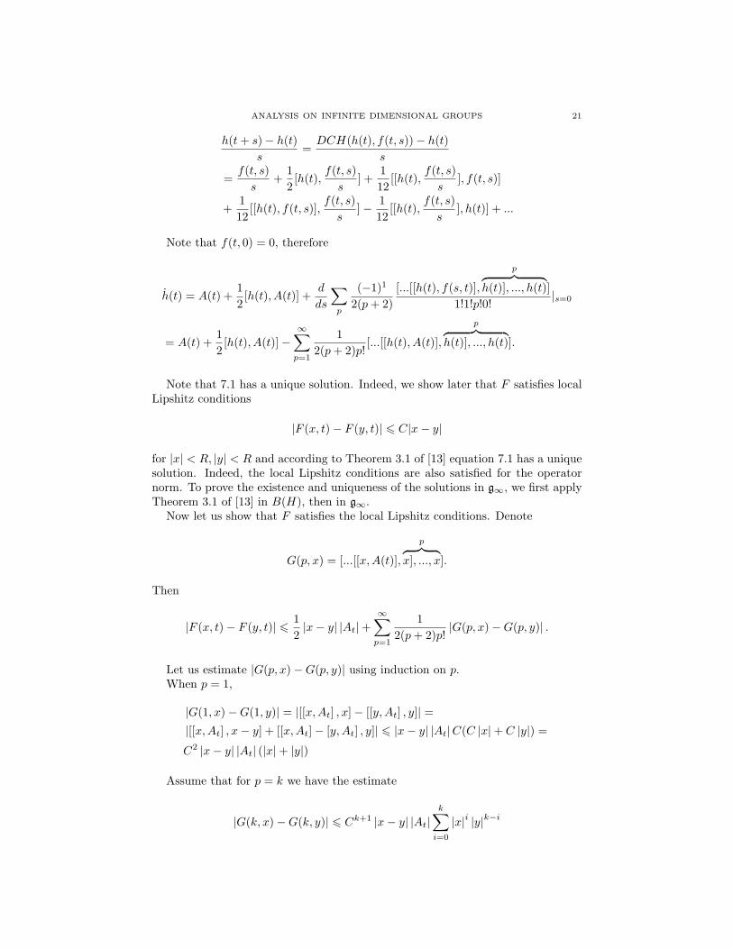
x], ..., x].(7.2)

Proof. Indeed, h(t + s)− h(t) = log g(t + s)− h(t) = log(g(t)g(t)−1g(t + s))− h(t).Denote f(t, s) = log(g(t)−1g(t+s)). Then h(t+s)−h(t) = log(eh(t)ef(t,s))−h(t) =DCH(h(t), f(t, s)) − h(t), where DCH(x, y) is given by the Dynkin-Campbell-Hausdorff formula for x, y ∈ g∞

(7.3) DCH(x, y) = log(exp x exp y)

=∑

m

∑

pi,qi

(−1)m−1

m(∑

ipi + qi)

[...

p1︷ ︸︸ ︷

[x, x], ..., x],

q1︷ ︸︸ ︷

y], ..., y],

qm︷ ︸︸ ︷

..., y], ...y]p1!q1!...pm!qm!

.

Thus

DCH(h(t), f(t, s)) = h(t) + f(t, s) +12[h(t), f(t, s)]

+112

[[h(t), f(t, s)], f(t, s)]− 112

[[h(t), f(t, s)], h(t)] + ...

Let us find df(t,s)ds |s=0.

f(t, s + ε)− f(t, s)ε

=log(g(t)−1g(t + s + ε))− log(g(t)−1g(t + s))

ε

=∞∑

n=1

(−1)n−1

n(g(t)−1g(t + s + ε)− I)n − (g(t)−1g(t + s)− I)n

ε

=∞∑

n=1

(−1)n−1

n1ε

n∑

k=1

(g(t)−1g(t + s + ε)− I)k−1

g(t)−1(g(t + s + ε)− g(t + s))(g(t)−1g(t + s)− I)n−k −−−→ε→0

∞∑

n=1

(−1)n−1

n

n∑

k=1

(g(t)−1g(t + s)− I)k−1g(t)−1g(t + s)(g(t)−1g(t + s)− I)n−k.

Thus

df(t, s)ds

|s=0 =∞∑

n=1

(−1)n−1

n

n∑

k=1

(g(t)−1g(t)− I)k−1g(t)−1g(t)(g(t)−1g(t)− I)n−k

= g(t)−1g = A(t).

ANALYSIS ON INFINITE DIMENSIONAL GROUPS 21

h(t + s)− h(t)s

=DCH(h(t), f(t, s))− h(t)

s

=f(t, s)

s+

12[h(t),

f(t, s)s

] +112

[[h(t),f(t, s)

s], f(t, s)]

+112

[[h(t), f(t, s)],f(t, s)

s]− 1

12[[h(t),

f(t, s)s

], h(t)] + ...

Note that f(t, 0) = 0, therefore

h(t) = A(t) +12[h(t), A(t)] +

dds

∑

p

(−1)1

2(p + 2)[...[[h(t), f(s, t)],

p︷ ︸︸ ︷

h(t)], ..., h(t)]1!1!p!0!

|s=0

= A(t) +12[h(t), A(t)]−

∞∑

p=1

12(p + 2)p!

[...[[h(t), A(t)],

p︷ ︸︸ ︷

h(t)], ..., h(t)].

Note that 7.1 has a unique solution. Indeed, we show later that F satisfies localLipshitz conditions

|F (x, t)− F (y, t)| 6 C|x− y|

for |x| < R, |y| < R and according to Theorem 3.1 of [13] equation 7.1 has a uniquesolution. Indeed, the local Lipshitz conditions are also satisfied for the operatornorm. To prove the existence and uniqueness of the solutions in g∞, we first applyTheorem 3.1 of [13] in B(H), then in g∞.

Now let us show that F satisfies the local Lipshitz conditions. Denote

G(p, x) = [...[[x,A(t)],

p︷ ︸︸ ︷

x], ..., x].

Then

|F (x, t)− F (y, t)| 6 12|x− y| |At|+

∞∑

p=1

12(p + 2)p!

|G(p, x)−G(p, y)| .

Let us estimate |G(p, x)−G(p, y)| using induction on p.When p = 1,

|G(1, x)−G(1, y)| = |[[x,At] , x]− [[y, At] , y]| =|[[x,At] , x− y] + [[x,At]− [y, At] , y]| 6 |x− y| |At|C(C |x|+ C |y|) =

C2 |x− y| |At| (|x|+ |y|)

Assume that for p = k we have the estimate

|G(k, x)−G(k, y)| 6 Ck+1 |x− y| |At|k

∑

i=0

|x|i |y|k−i

22 MARIA GORDINA

Then for p = k + 1 we have|G(k + 1, x)−G(k + 1, y)| = |[G(k, x), x]− [G(k, y), y]|= |[G(k, x), x]− [G(k, x), y] + [G(k, x), y]− [G(k, y), y]|6 C |G(k, x)| |x− y|+ C |G(k, x)−G(k, y)| |y|

6 Ck+2 |x|k+1 |At| |x− y|+ Ck+2 |x− y| |At|

(

k∑

i=0

|x|i |y|k−i

)

|y|

= Ck+2 |x− y| |At|k+1∑

i=0

|x|i |y|k+1−i .

Thus if |x| 6 R, |y| 6 R

|G(p, x)−G(p, y)| 6 Cp+1 |x− y| |At|Rp(p + 1)

and therefore

|F (x, t)− F (y, t)| 6 12|x− y| |At|+

∞∑

p=1

12(p + 2)p!

Cp+1 |x− y| |At|Rp(p + 1)

612|x− y| |At|+

12|x− y| |At|C

∞∑

p=1

CpRp

p!=

12|x− y| |At| (1 + C(eCR − 1)).

Lemma 7.4. There are constants C1, C2 and 0 < ε < ln 2/2C such that

C1 |x− y| 6 d(exp x, exp y) 6 C2 |x− y|for any x, y ∈ g∞ provided |x| < ε, |y| < ε.

Proof. Take a path g : [0, 1] → exp(g∞) such that g(0) = ex, g(1) = ey. Leth = log g. Then

g−1g =∞∑

k=0

(−adh)k(h)(k + 1)!

= h− [h, h] +[h, [h, h]]

2!− [h, [h, [h, h]]]

3!+ ...

1. First prove that d(exp x, exp y) 6 C2 |x− y|:

|g−1g| 6 |h|∞∑

k=0

Ck|h|k

k!= |h|eC|h|

=⇒ d(exp x, exp y) = infg

∫ 1

0|g−1g|ds 6 inf

h

∫ 1

0|h|eC|h|ds.

Take h(s) = xs + (1− s)y

d(exp x, exp y) 6∫ 1

0|x− y|eC(|x|s+(1−s)|y|)ds = |x− y|

∫ 1

0eC(|x|−|y|)seC|y|ds

= |x− y|eC|y| eC(|x|−|y|) − 1C(|x| − |y|)

= |x− y|eC|x| − eC|y|

C(|x| − |y|)6 |x− y|eC max|x|,|y|,

since ea−eb

a−b 6 emax|a|,|b|. Thus

d(exp x, exp y) 6 |x− y|eC max|x|,|y| 6 |x− y|eCε.

ANALYSIS ON INFINITE DIMENSIONAL GROUPS 23

2. Now let us prove that C1 |x− y| 6 d(exp x, exp y):

|g−1g| = |∞∑

k=0

(−adh)k(h)(k + 1)!

| > |h|

(

1−∞∑

k=1

|h|kCk

k!

)

= |h|

(

1−∞∑

k=0

|h|kCk

k!+ 1

)

= |h|(

2− eC|h|)

.

Consider two cases.2a. Suppose max

s|h(s)| < 2ε. Then

∫ 1

0|g−1g|ds >

∫ 1

0|h|

(

2− eC|h|)

ds

>(

2− e2εC)

∫ 1

0|h|ds >

(

2− e2εC)

|∫ 1

0hds| =

(

2− e2εC)

|x− y|.

2b. Take a path h such that maxs|h(s)| > 2ε. Denote t1 = mint : |h(t)| = ε,

t2 = mint : |h(t)| = 2ε. Note that t1 < t2 since h(0) = x and |x| < ε. Then∫ 1

0|g−1g|ds >

∫ t2

t1|g−1g|ds

>∫ t2

t1|h|

(

2− eC|h|)

ds >(

2− e2εC)

∫ t2

t1|h|ds >

(

2− e2εC)

|h(t2)− h(t1)|

> ε(

2− e2εC)

>|x− y|

2(

2− e2εC)

.

2a and 2b imply that

d(exp x, exp y) = infg

∫ 1

0|g−1g|ds >

|x− y|2

(

2− e2εC)

.

Lemma 7.5. Take g(t) : [0, 1] → GCM , g ∈ C1CM . Suppose that g(0) = e, ‖g(t)−

e‖ < 1 for any t ∈ [0, 1] and | log g(1)| < ε, where ε is the same as in Lemma 7.4.Then g(1) ∈ G∞.

Proof. Let h = log g =∞∑

n=1((−1)n−1/n)(g(t) − I)n. Then by Lemma 7.3 h is a

unique solution in g∞ of the ordinary differential equation 7.1. In particular, itimplies that g(t) ∈ g∞. Therefore, there are Hn ∈ gn (projections of h(1) onto gn)such that |h(1)−Hn| −−−→

n→∞0.

By Lemma 7.4

d(eh(1), eHn) 6 C2|h(1)−Hn|.

A similar estimate holds for dn instead of d. By a direct calculation eh(t) = g(t).Thus g(1) ∈ G∞, since eHn ∈ Gn.

Proof of Theorem 7.2. 1. G∞ ⊆ GCM since Gn ⊆ GCM for all n and G∞ isclosed in the metric d∞.

Now we will show that GCM ⊆ G∞.

24 MARIA GORDINA

Take A ∈ G∞, B ∈ GCM , a path g : [0, 1] → GCM , g ∈ C1CM , g(0) = A, g(1) =

B. We want to show that B ∈ G∞.Lemma 7.5 proves this in a neighborhood of I. Prove it for a neighborhood of

any element of G∞. Suppose ‖g(t)−A‖ < 1, d(log B, log A) < ε.For any δ > 0 there is Cδ ∈

⋃

nGn such that d(A, Cδ) < δ. Thus

d(B, Cδ) 6 d(B, A) + d(A,Cδ) < ε + δ.

Therefore d(C−1δ B, e) < ε + δ, so by part 1 C−1

δ B ∈ G∞. This means that thereis Dδ ∈

⋃

nGn such that

d(C−1δ B,Dδ) < δ.

Now d(C−1δ B,Dδ) = d(B,CδDδ) < δ,CδDδ ∈

⋃

nGn. This proves that B ∈ G∞.

Now take any A,B and a path g joining them. Divide log g into subpaths satis-fying the conditions in the first part of the proof.2. By Lemma 7.3 and Lemma 7.4 exp and log are well defined and differentiable inneighborhoods of the identity and zero respectively.

8. Holomorphic polynomials and skeletons

Definition 8.1. A function p : I + HS −→ C is called a holomorphic polynomial,if p is a complex linear combination of finite products of monomials pm,l

k (X) =(〈Xfm, fl〉)k, where fm∞m=1 is an orthonormal basis of H. We will denote thespace of all such polynomials by HP.

These polynomials are holomorphic because the kth derivative (DkXp)(β) exists

and is complex linear for any p ∈ P, X ∈ I + HS, β ∈ g⊗k∞ . Indeed, let ξ be any

element of g∞, then the derivative of pm,lk in the direction of ξ is (Dpm,l

k )(X)(ξ) =kpm,l

1 (Xξ)pm,lk−1(X). From this formula we can see that Dpm,l

k (X)(ξ) is complexlinear in ξ.

Remark 8.2. Any polynomial p ∈ HP can be written in the form p(X) =m∑

k=1

∏nml=1 Tr(AklX)

for some Akl ∈ HS. The converse is not true in general, but the closure in

L2(I + HS, µt) of all functions of the formm∑

k=1

∏nml=1 Tr(AklX) coincides with

the closure of holomorphic polynomials. Therefore the next definition is basis-independent, though the definition of HP depends on the choice of fk∞k=1.

Definition 8.3. The closure of all holomorphic polynomials in L2(I + HS, µt) iscalled HL2(I + HS, µt).

Lemma 8.4. (B. Driver’s formula).Let g be a smooth path in GCM such that g(0) = I and g ∈ C1

CM . Then for anyp ∈ HP

p(g(s)) =∞∑

n=0

∫

∆n(s)

(Dnp)(I)(c(s1)⊗ ...⊗ c(sn))d~s,

where

∆n(s) = (s1, ..., sn) ∈ Rn : 0 6 s1 6 s2... 6 sn 6 s, c(s) = g−1(s)dgds

.

ANALYSIS ON INFINITE DIMENSIONAL GROUPS 25

Proof. Take a monomial p(x) = (〈Xfm, fl〉)k, deg p = k. Similarly to Lemma 5.2of [4]

p(g(s)) =N−1∑

n=0

∫

∆n(s)

(Dnp)(I)(c(s1)⊗ ...⊗ c(sn))d~s

+∫

∆N (s)

(DNp)(g(s1))(c(s1)⊗ ...⊗ c(sN ))d~s.

We want to estimate the remainder∣

∣

∣

∫

∆N (s)

(DNp)(g(s1))(c(s1)⊗ ...⊗ c(sN ))d~s∣

∣

∣

6∫

∆N (s)

∣

∣(DNp)(g(s1))(c(s1)⊗ ...⊗ c(sN ))∣

∣ d~s.

Note that if k = deg p 6 N then

(DNp)(X)(ξ1 ⊗ ...⊗ ξN ) =∑

p1(X~ξα1)p1(X~ξα2) · ... · p1(X~ξαi) · ... · p1(X~ξαk),

where αi = 〈ai1, ..., a

iN 〉, ai

j = 0 or 1, ~ξαi = ξai1

1 ...ξaiN

N ,k∑

i=1αi = 〈1, ..., 1〉, p1(Y ) =

〈Xfm, fl〉 and the sum is taken over all possible α = (α1, ..., αk).For ξ ∈ HS, X ∈ I + HS

|p1(Xξ)| 6 (‖(X − I)ξ‖HS + ‖ξ‖HS) 6 ‖ξ‖HS(‖(X − I‖HS + 1).

The number of all such α is kN therefore∣

∣(DNp)(X)(ξ1 ⊗ ...⊗ ξN )∣

∣ 6 ‖ξ1‖HS ...‖ξN‖HS(‖(X − I‖HS + 1)kN .

Denote

‖c‖1 =

1∫

0

|c(t)|dt.

Thus∫

∆N (s)

∣

∣(DNp)(g(s1))(c(s1)⊗ ...⊗ c(sN ))∣

∣ d~s

6 ‖c‖N1 sup

06t6s(‖(g(t)− I‖HS + 1)kkN

∫

∆N (s)

d~s

= ‖c‖N1 sup

06t6s(‖(g(t)− I‖HS + 1)kkN sN

N !−−−−→N→∞

0.

Similarly we can prove this formula for any holomorphic polynomial.

26 MARIA GORDINA

Theorem 8.5. Suppose

pnL2(I+HS,µt)−−−−−−−−→

n→∞f, pn ∈ HP.

Then there is a holomorphic function f , a skeleton of f , on GCM such that

pn(x) → f(x) for any x ∈ GCM .

Proof. As we know from Theorem 4.4 the map (1 − D)−1I is an isometry from

HL2(I + HS, µt) to J0t . Thus (1 − D)−1

I pn converges in J0t to some α =

∑

αn.Define

f(x) =∞∑

n=0

∫

∆n(1)

αn(c(s1)⊗ ...⊗ c(sn))d~s.

Take a path g : [0, 1] → GCM , g(0) = e, g(1) = X. By Lemma 8.4

pm(X) =∞∑

n=0

∫

∆n(1)

(Dnpm)(I)(c(s1)⊗ ...⊗ c(sn))d~s,

so

|pm(X)− f(x)| 6∞∑

n=0

∫

∆n(1)

|((Dnpm)(I)− αn)(c(s1)⊗ ...⊗ c(sn))|d~s

6∞∑

n=0

∫

∆n(1)

|(Dnpm)(I)− αn||c(s1)⊗ ...⊗ c(sn)|d~s

6∞∑

n=0

|(Dnpm)(I)− αn|∫

∆n(1)

|c(s1)⊗ ...⊗ c(sn)|d~s.

Thus

|pm(X)− f(x)| 6∞∑

n=0

|(Dnpm)(I)− αn|‖c‖n

1

n!

=∞∑

n=0

|(Dnpm)(I)− αn|tn/2√

n!‖c‖n

1√n!tn/2

6

( ∞∑

n=0

|(Dnpm)(I)− αn|2tn

n!

)( ∞∑

n=0

‖c‖2n1

n!tn

)

= ‖(Dpm)(I)− α‖2t e‖c‖21/t −−−−→

m→∞0.

Now we will show that f is holomorphic. Take ξ ∈ g, g ∈ C1CM , g(0) = e, g(1) =

X. Define two paths in GCM

g1(s) =

g(s), 0 6 s 6 1g(1), 1 6 s 6 1 + t

g2(s) =

g(s), 0 6 s 6 1g(1)e(s−1)ξ, 1 6 s 6 1 + t

ANALYSIS ON INFINITE DIMENSIONAL GROUPS 27

Let c(s) = g−1(s)dgds ; then

c1(s) = g−11 (s)

dg1

ds=

c(s), 0 6 s 6 10, 1 6 s 6 1 + t

c2(s) = g−12 (s)

dg2

ds=

c(s), 0 6 s 6 1ξ, 1 6 s 6 1 + t

Then by the definition of f

f(Xetξ)− f(X) =∞∑

n=0

∫

∆n(1+t)

αn(c1(s1)⊗ ...⊗ c1(sn)− c2(s1)⊗ ...⊗ c2(sn))d~sn

=∞∑

n=0

1+t∫

1

∫

∆n−1(sn)

αn(c1(s1)⊗ ...⊗ c1(sn)− c2(s1)⊗ ...⊗ c2(sn))d~sn−1dsn

=∞∑

n=0

∫

∆n−1(1)

αn(c(s1)⊗ ...⊗ c(sn−1)⊗ tξ)d~sn−1

+∞∑

n=0

1+t∫

1

sn∫

1

∫

∆n−2(sn−1)

αn(c1(s1)⊗ ...⊗ c1(sn)− c2(s1)⊗ ...⊗ c2(sn))d~sn−2dsn−1dsn

=∞∑

n=0

t∫

∆n−1(1)

αn(c(s1)⊗ ...⊗ c(sn−1)⊗ ξ)d~sn−1

+∞∑

n=0

1+t∫

1

sn∫

1

∫

∆n−2(sn−1)

αn(c(s1)⊗ ...⊗ c(sn−2 ⊗ ξ ⊗ ξ)d~sn−2dsn−1dsn.

Thus∣

∣

∣

∣

∣

∣

∣

f(Xetξ)− f(X)t

−∫

∆n−1(1)

αn(c(s1)⊗ ...⊗ c(sn−1)⊗ ξ)d~sn−1

∣

∣

∣

∣

∣

∣

∣

6

1t

1+t∫

1

(sn − 1)∫

∆n−2(sn−1)

αn(c(s1)⊗ ...⊗ c(sn−2 ⊗ ξ ⊗ ξ)d~sn−2dsn−1dsn −−−→n→0

0

since 0 6 sn − 1 6 t.This means that the derivative of f at X in the direction ξ is

(ξf)(X) =∫

∆n−1(1)

αn(c(s1)⊗ ...⊗ c(sn−1)⊗ ξ)d~sn−1

and it is complex linear.

Remark 8.6. The convergence is uniform on bounded sets. In fact, one can showthat the derivatives also converge uniformly on bounded sets.

Theorem 8.7. 1. HP ⊂ Lp(I + HS, µt), for any p > 1.

28 MARIA GORDINA

2. ‖f‖t,n −−−→n→∞

‖f‖t for any f ∈ HP.

3. The embedding of HP into Ht(G∞) can be extended to an isometry fromHL2(I + HS, µt) into Ht(G∞).

Proof. 1.∫

I+HS

|pm,lk (X)|pµt(dX) = E|pm,l

k (Yt + I)|p = E|(Yt)ml + δml)|pk

6 E2pk−1(|(Yt)ml|pk + 1) 6 2pk−1E(‖Yt‖pkHS + 1) < ∞

by Lemma 5.7. Thus HP ⊂ Lp(I + HS, µt) for any p > 1.

2. From the estimate on E‖Yt‖pHS in Proposition 5.6 we can find C(p, t) such

that ‖|p|2‖t,n(k) 6 C(p, t) for any k. Then apply Lemma 5.7 to f = |p|2.

3. By part 1 of Theorem 8.7 HP ⊂ L2(I + HS, µt). In addition, by part 2 ofTheorem 8.7

‖p‖t,n −−−→n→∞

‖p‖t, p ∈ HP.

Therefore ‖p‖t,∞ = ‖p‖t and so the embedding is an isometry.The space HL2(I +HS, µt) is the closure of HP, therefore the isometry extends

to it from HP.

Remark 8.8. If f is an element of HL2(I + HS, µt), g is its image under theisometry in this theorem and f is the skeleton of f , then f |G∞ = g.

Corollary 8.9. The space Ht(G∞) is an infinite dimensional Hilbert space.

9. Examples

Denote HSn×n = A : 〈Afm, fk〉 = 0 if max(m, k) > n. Take a basis ek∞k=1

of HS such that ek2n2

k=1 is a basis of HSn×n. By BT we will denote the transposeof the operator B, i. e. BT = (ReB)∗ + i(ImB)∗.

Example 9.1. We begin with the definition of the Hilbert-Schmidt complex or-thogonal group.

Definition 9.1. The Hilbert-Schmidt complex orthogonal group SOHS is the con-nected component containing the identity I of the group OHS = B : B − I ∈HS, BT B = BBT = I. The Lie algebra of skew-symmetric Hilbert-Schmidt oper-ators will be denoted by soHS = A : A ∈ HS, AT = −A.

Let Q be a symmetric positive trace class operator on soHS and let the innerproduct be defined by 〈A,B〉 = 〈Q−1/2A,Q−1/2B〉HS . In [7] we showed that if Q isthe identity operator, then all Hilbert spaces we consider are isomorphic to C; thatis, there are no nonconstant holomorphic functions. As in Section 5 we identify Qwith its extension by 0 to the orthogonal complement of soHS .

Define groups Gn = SO(n,C) = B ∈ SOHS , B − I ∈ HSn×n. These groupsare isomorphic to the special complex orthogonal group of Cn. Their Lie algebrasare Lie(SO(n,C)) = so(n,C) = A ∈ HSn×n, AT = −A with an inner product〈A,B〉n = 〈(PnQPn)−1/2A, (PnQPn)−1/2B〉HS . Here Pn = Pso(n,C). We assumethat all so(n,C) are invariant subspaces of Q. The groups SO(n,C) are not simplyconnected, therefore we have isometries from Ht(SO∞) and HL2(I+HS, µt) to J0

t ,

ANALYSIS ON INFINITE DIMENSIONAL GROUPS 29

but not an isomorphism between Ht(SO∞) and J0t . In addition to the properties of

the heat kernel measure described in this paper, we showed in [7] that the processYt + I actually lives in the group SOHS .

Example 9.2. The Hilbert-Schmidt complex symplectic group is defined similarlyto the Hilbert-Schmidt complex orthogonal group.

Definition 9.2. The Hilbert-Schmidt complex symplectic group SpHS is the group

of operators X =(

A BC D

)

such that A − I, D − I, B,C ∈ HS and XT JX = J ,

where J =(

0 −II 0

)

. The Lie algebra is spHS = X =(

A BC D

)

: A,B, C,D ∈

HS, XT J + JX = 0.

The corresponding finite dimensional groups are isomorphic to the classical sym-

plectic complex groups Sp(n,C) = X =(

A BC D

)

∈ SpHS , A − I, D − I, B, C ∈

HSn×n with Lie algebras sp(n,C) = X =(

A BC D

)

∈ spHS : A,B, C,D ∈

HSn×n. An inner product on spHS and sp(n,C) is defined in the same way as inExample 9.1. Similarly to soHS if Q is the identity operator, the corresponding J t

0is trivial by Theorem 4.6. The groups Sp(n,C) are simply connected; therefore theisometry from Ht(Sp∞) to J0

t is surjective. Similar to SOHS the process Yt + Ilives in SpHS .

Statement 9.3. Yt + I lies in SpHS for any t > 0 with probability 1.

Proof. We need to check that (Yt + I)J(Yt + I)T = J with probability 1 for anyt > 0. To do this we will apply Ito’s formula to G(Yt), where G is defined as follows:G(Y ) = Λ(Y JY T + Y J + JY T ), Λ is a linear real bounded functional from HS toR.

In order to use Ito’s formula we must verify several properties of the process Yt

and the mapping G:1. B(Ys) is an L0

2-valued process stochastically integrable on [0, T ].2. G and the derivatives Gt, GY , GY Y are uniformly continuous on bounded

subsets of [0, T ]×HS.

Proof of 1. See 1 in the proof of Theorem 5.1.

Proof of 2. Let us calculate Gt, GY , GY Y . First of all, Gt = 0. For any S ∈ HS

GY (Y )(S) = Λ(SJY T + Y JST + SJ + JST ).

For any S, T ∈ HS

GY Y (Y )(S ⊗ T ) = Λ(SJTT + TJST ).

Thus condition 2 is satisfied.We will use the notation:

GY (Y )(S) = 〈GY (Y ), S〉HS ,

GY Y (Y )(S ⊗ T ) = 〈GY Y (Y )S, T 〉HS ,

where GY is an element of HS and GY Y is an operator on HS corresponding tothe functionals GY ∈ HS∗ and GY Y ∈ (HS ⊗HS)∗.

30 MARIA GORDINA

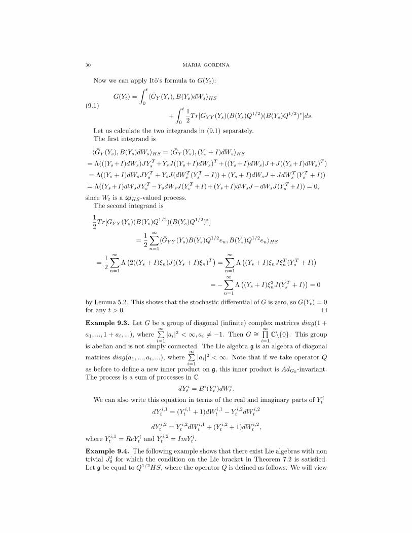
Now we can apply Ito’s formula to G(Yt):

G(Yt) =∫ t

0〈GY (Ys), B(Ys)dWs〉HS

+∫ t

0

12Tr[GY Y (Ys)(B(Ys)Q1/2)(B(Ys)Q1/2)∗]ds.

(9.1)

Let us calculate the two integrands in (9.1) separately.The first integrand is

〈GY (Ys), B(Ys)dWs〉HS = 〈GY (Ys), (Ys + I)dWs〉HS

= Λ(((Ys +I)dWs)JY Ts +YsJ((Ys +I)dWs)T +((Ys +I)dWs)J +J((Ys +I)dWs)T )

= Λ((Ys + I)dWsJY Ts + YsJ(dWT

s (Y Ts + I)) + (Ys + I)dWsJ + JdWT

s (Y Ts + I))

= Λ((Ys +I)dWsJY Ts −YsdWsJ(Y T

s +I)+(Ys +I)dWsJ−dWsJ(Y Ts +I)) = 0,

since Wt is a spHS-valued process.The second integrand is

12Tr[GY Y (Ys)(B(Ys)Q1/2)(B(Ys)Q1/2)∗]

=12

∞∑

n=1

〈GY Y (Ys)B(Ys)Q1/2en, B(Ys)Q1/2en〉HS

=12

∞∑

n=1

Λ(

2((Ys + I)ξn)J((Ys + I)ξn)T )

=∞∑

n=1

Λ(

(Ys + I)ξnJξTn (Y T

s + I))

= −∞∑

n=1

Λ(

(Ys + I)ξ2nJ(Y T

s + I))

= 0

by Lemma 5.2. This shows that the stochastic differential of G is zero, so G(Yt) = 0for any t > 0.

Example 9.3. Let G be a group of diagonal (infinite) complex matrices diag(1 +

a1, ..., 1 + ai, ...), where∞∑

i=1|ai|2 < ∞, ai 6= −1. Then G ∼=

∞∏

i=1C\0. This group

is abelian and is not simply connected. The Lie algebra g is an algebra of diagonal

matrices diag(a1, ..., ai, ...), where∞∑

i=1|ai|2 < ∞. Note that if we take operator Q

as before to define a new inner product on g, this inner product is AdGR -invariant.The process is a sum of processes in C

dY it = Bi(Y i

t )dW it .

We can also write this equation in terms of the real and imaginary parts of Y it

dY i,1t = (Y i,1

t + 1)dW i,1t − Y i,2

t dW i,2t

dY i,2t = Y i,2

t dW i,1t + (Y i,2

t + 1)dW i,2t ,

where Y i,1t = ReY i

t and Y i,2t = ImY i

t .

Example 9.4. The following example shows that there exist Lie algebras with nontrivial J t

0 for which the condition on the Lie bracket in Theorem 7.2 is satisfied.Let g be equal to Q1/2HS, where the operator Q is defined as follows. We will view

ANALYSIS ON INFINITE DIMENSIONAL GROUPS 31

the elements of HS as infinite matrices. Denote by eij an infinite matrix whoseentries are all zero except the one equal to 1 at the intersection of the ith row andjth column. These matrices form an orthonormal basis of HS. We assume that Qis diagonal in this basis, namely, Qeij = e−(i+j)eij . Note that this Q is a positivetrace class operator, so we can construct the corresponding heat kernel measure.Thus the space Ht(G∞) contains all holomorphic polynomials and therefore thespace J t

0 is not trivial. Now let us verify that the condition on the Lie bracket issatisfied. For any x and y in g

|xy|2 =∑

i,m

ei+m

∑

j

xi,jyj,m

2

=∑

i,m

∑

j

e−je12 (i+j)xi,je

12 (j+m)yj,m

2

6∑

i,m

∑

j

e12 (i+j)xi,je

12 (j+m)yj,m

2

6∑

i,m

∑

j

ei+jx2i,j

(

∑

k

ek+my2k,m

)

=∑

i,j

ei+jx2i,j

∑

m,k

ek+mx2m,k = |x|2|y|2.

Thus |[x, y]| 6 2|x||y|. A similar construction can be done for the algebras consid-ered in Example 9.1 and Example 9.2.

References

[1] V.Bargmann, On a Hilbert space of analytic functions and an associated integral transform,Part I, Communications of Pure and Applied Mathematics, 24, 1961, 187-214.

[2] V.Bargmann, Remarks on a Hilbert space of analytic functions, Proc. of the National Acad-emy of Sciences, 48, 1962, 199-204.

[3] G.DaPrato and J.Zabczyk, Stochastic Equations in Infinite Dimensions, Cambridge Univer-sity Press,Cambridge,1992.

[4] B.Driver, On the Kakutani-Ito-Segal-Gross and Segal-Bargmann-Hall isomorphisms, J. ofFunct. Anal., 133,1995,69-128.

[5] B.Driver and L.Gross, Hilbert spaces of holomorphic functions on complex Lie groups,Proceedings of the 1994 Taniguchi International Workshop (K. D. Elworthy, S. Kusuoka,I. Shigekawa, Eds.), World Scientific Publishing Co. Pte. Ltd, Singapore/New Jer-sey/London/Hong Kong, 1997.

[6] E. B. Dynkin, Calculation of the coefficients in the Campbell-Hausdorff formula, DokladyAkad. Nauk SSSR (N.S.) 57, 1947, 323-326.

[7] M. Gordina, Holomorphic functions and the heat kernel measure on an infinite dimensionalcomplex orthogonal group, to appear in Potential Analysis.

[8] L. Gross and P. Malliavin, Hall’s transform and the Segal-Bargmann map, Ito’s StochasticCalculus and Probability Theory, (M.Fukushima, N. Ikeda, H. Kunita and S. Watanabe,Eds.), Springer-Verlag, New York/Berlin, 1996.

[9] B.Hall, The Segal-Bargmann ’coherent state’ transform for compact Lie groups, J. of Funct.Anal., 122, 1994, 103-151.

[10] B. Hall and A. Sengupta, The Segal-Bargmann transform for path-groups, J. of Funct. Anal.,152, 1998, 220-254.

[11] O. Hijab, Hermite functions on compact Lie groups I, J. of Funct. Anal., 125, 1994, 480-492.[12] O. Hijab, Hermite functions on compact Lie groups II, J. of Funct. Anal., 133, 1995, 41-49.[13] Robert H. Martin, Jr., Nonlinear operators and differential equations in Banach spaces,

Pure and Applied Mathematics. Wiley-Interscience [John Wiley & Sons], New York-London-Sydney, 1976.

[14] I. Shigekawa, Ito-Wiener expansions of holomorphic functions on the complex Wiener space,in Stochastic Analysis, (E. Mayer et al, Eds.), Academic Press, San Diego, 1991, 459-473.

32 MARIA GORDINA

[15] H.Sugita, Properties of holomorphic Wiener functions-skeleton, contraction, and local Taylorexpansion, Probab. Theory Related Fields, 100, 1994, 117–130.

[16] H.Sugita, Regular version of holomorphic Wiener function, J. Math. Kyoto Univ., 34, 1994,849–857.

Department of Mathematics and Statistics, McMaster University, Hamilton, ON L8S4K1 Canada

E-mail address: gordina@math.McMaster.ca