Page 1
HEAT TRANSFER ACCURACY STUDY FOR HYPERSONIC FLOW USING
OVERSET MESH
by
ERIK GUNAWAN WINARDI
ROY P. KOOMULLIL, COMMITTEE CHAIR
GARY CHENG
ROBERT NICHOLS
A THESIS
Submitted to the graduate faculty of The University of Alabama at Birmingham,
in partial fulfillment of the requirements for the degree of
Master of Science
BIRMINGHAM, ALABAMA
2010
Page 2
ii
EVALUATION OF DIFFERENT FLUX SCHEMES FOR HYPERSONIC FLOWS
USING GENERALIZED OVERSET MESH
ERIK GUNAWAN WINARDI
MASTER OF SCIENCE IN MECHANICAL ENGINEERING
ABSTRACT
An accurate prediction of aerodynamic heating is critical to the design of a
Thermal Protection System (TPS) for hypersonic vehicles. It however remains a
challenging task as the majority of Riemann solver based shock capturing schemes suffer
from the “carbuncle” phenomenon. A new adaptive scheme approach based on the
Riemann solver called HLLC+ was implemented in the in-house computational fluid
dynamics solver for generalized meshes to improve the accuracy of solution in
hypersonic simulation. Study of different convective fluxes was performed with
generalized single mesh approach. In addition, generalized meshes with an overset
framework were used to study the effect of numerical flux calculations, mesh topology,
overset interpolation approach, and mesh resolution on heat transfer predictions for high
speed flows. A library based approach was used for the calculation of domain
connectivity information and data communication between overlapping meshes. The
results indicated that a high dissipative Riemann solver could prevent the „carbuncle‟
phenomenon at the expense of solution accuracy at the boundary layer region. The
adaptive scheme HLLC+ proved to be an effective approach for preventing the
occurrence of carbuncle. Furthermore, the use of a small resolution non-dimensional wall
distance (y+) resulted in more accurate heat transfer prediction. It is concluded that both
Page 3
iii
accurate numerical scheme and non-dimensional wall distance are the most important
factors that affect the heat transfer prediction accuracy.
Page 4
iv
ACKNOLEDGEMENT
I would like to thank you my advisor Dr. Roy Koomullil for guiding me in
learning the fundamental of computational fluid dynamics and giving me the opportunity
in doing research in the field. I would like also to thank you my committee members Dr.
Gary Cheng and Dr. Robert Nichols for their incredible guidance in finishing my research
thesis. I would also want to thank to all the professors and staffs at mechanical
engineering department for their patient to assist me in my learning process at the
university.
I would like to thank all my friends that I encountered during my study at
University of Alabama at Birmingham. Special thanks to Balaji, Nitin, and Sandeep for
their invaluable help and guidance during my study. I would also thank to my roommate
Il Hwan Kim for his supports and accompany for more than two years in Birmingham.
Finally, I would like to give a special thank to my family. My father, dr.
Tjahjanegara Winardi and my mother, dr Lenny Gunawan for all their support and love. I
also appreciate the support from my brother, Andreas Winardi, my sister in law Amelia
Irawan, and also their daughter Allie for entertaining me since the day she was born last
year.
Page 5
v
LIST OF TABLES
Table 1.1. Advantages and Disadvantages of Four Meshing Methods. ............................... 4
Table 4.1. Initial Condition for Shock Tube Problems. ....................................................... 30
Table 4.2. Mesh Information for Overset Meshes with Different Topology. .................... 63
Table 4.3. Structure-Structure Overset Mesh with Different y+ to the Wall Information.
................................................................................................................................................. 64
Page 6
vi
LIST OF FIGURES
Figure 2.1. Types of Flux Splitting Schemes. ........................................................................ 8
Figure 2.2. Shock Dissipation at Cells Differs at Tangential Face (A-B, C-D) and at
Normal Face (A-C, B-D). ........................................................................................................ 9
Figure 2.3. Effect of Cell Aspect Ratio and Carbuncle. ...................................................... 11
Figure 2.4. Overset Mesh Method Assembly. ...................................................................... 13
Figure 3.1. Shock-tube Problem. ........................................................................................... 20
Figure 3.2. Riemann Problems at Each Interface. ................................................................ 21
Figure 3.3. One Intermediate State of HLL and HLLE Riemann Fan. ............................... 22
Figure 3.4. Two Intermediate States of The HLLC Riemann Fan. ..................................... 24
Figure 4.1. Carbuncle Phenomenon for Flow over a Hypersonic Cylinder. ...................... 29
Figure 4.2. Comparison of Computed and Exact Solution for Test 1 at Time 0.2. ........... 32
Figure 4.3. Comparison of Computed and Exact Solution for Test 2 at Time 0.15. ......... 34
Figure 4.4. Comparison of Computed and Exact Solution for Test 3 at Time 0.012. ....... 35
Figure 4.5. Comparison of Computed and Exact Solution for Test 4 at Time 0.035. ....... 37
Figure 4.6. Comparison of Computed and Exact Solution for Test 5 at Time = 0.012. .... 38
Figure 4.7. Results from Mesh Resolution Study using HLLC scheme. ............................ 40
Figure 4.8. Results from Mesh Resolution Study using HLLE scheme. ............................ 41
Figure 4.9. Results from Mesh Resolution Study using HLLC+ scheme. ......................... 42
Figure 4.10. Shock Tube Test 4 with 100 Mesh Points in x Direction. .............................. 44
Figure 4.11. Shock Tube Test 4 with 200 Mesh Points in x Direction. .............................. 45
Figure 4.12. Shock Tube Test 4 with 400 Mesh Points in x Direction. .............................. 47
Figure 4.13. Mesh used for Ramp Testcase and the Location of the Line of Interest. ...... 48
Page 7
vii
Figure 4.14. Density Distribution for Ramp Testcase. ........................................................ 49
Figure 4.15. Density Contour for Combination HLLC+ with Different Delta Values. ..... 50
Figure 4.16. The Density Values Inside the Shock Region. ................................................ 50
Figure 4.17. Density Plot for Different Delta Values for HLLC+ Scheme. ....................... 51
Figure 4.18. Density Plot Comparison for HLLE, Roe-HLLE, and HLLC+ Scheme. ...... 51
Figure 4.19. Comparison of Pressure Contour from Simulations using Different Flux
Evaluations. ............................................................................................................................ 53
Figure 4.20. Comparison of Pressure Distribution on the Cylinder Surface. ..................... 54
Figure 4.21. The Location of Region of Interest for Cylinder case. ................................... 55
Figure 4.22. Pressure Distribution accros the Line of Interest at 0 degree ......................... 56
Figure 4.23. Closer Look of Pressure Distribution accros the Line of Interest at 0 degree.
................................................................................................................................................. 56
Figure 4.24. Simulation of Moving Shock on Overset Mesh Assembly. ........................... 58
Figure 4.25. Simulations of Shock Wedge Interaction using Overset Meshes. ................. 58
Figure 4.26. Overset Grid Assembly for Structured Background and Body Fitted Meshes.
................................................................................................................................................. 59
Figure 4.27. Overset Mesh with Structured Background Mesh and Hybrid Body Fitted
Mesh and Pressure Distribution from the Simulation. ......................................................... 61
Figure 4.28. Coefficient of Pressure across the Cylinder Surface for Different
Interpolation Scheme. ............................................................................................................ 62
Figure 4.29. Pressure Distribution using Overset Meshes with Different Mesh
Topologies. ............................................................................................................................. 63
Page 8
viii
Figure 4.30. Comparison of Pressure Distribution from Overset Meshes with Different
Mesh. ....................................................................................................................................... 64
Figure 4.31. Shock/Shock Interactions Experimental Set Up at ONERA.......................... 65
Figure 4.32. Pressure Contour for Shock/Shock Interaction Study with 20o Shock
Generator. ............................................................................................................................... 66
Figure 4.33. Pressure Contour for Shock/Shock Interaction Study with 22o Shock
Generator. ............................................................................................................................... 67
Figure 4.34. Close View at the Shock/Shock Interaction Patterns. .................................... 68
Figure 4.35. Pressure Distribution on a Cylinder Surface. .................................................. 68
Figure 4.36. Heat Transfer Distribution on a Cylinder Surface. ......................................... 69
Figure 5.1. Comparison of Heat Flux Distribution on the Cylinder Surface. .................... 73
Figure 5.2. Comparison of Heat Flux Predictions from Different Interpolation
Techniques. ............................................................................................................................. 73
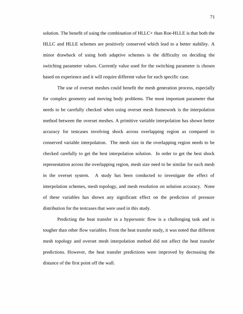
Figure 5.3. . Comparison of Heat Flux Predictions using Overset Meshes with Different
Mesh Topologies. ................................................................................................................... 74
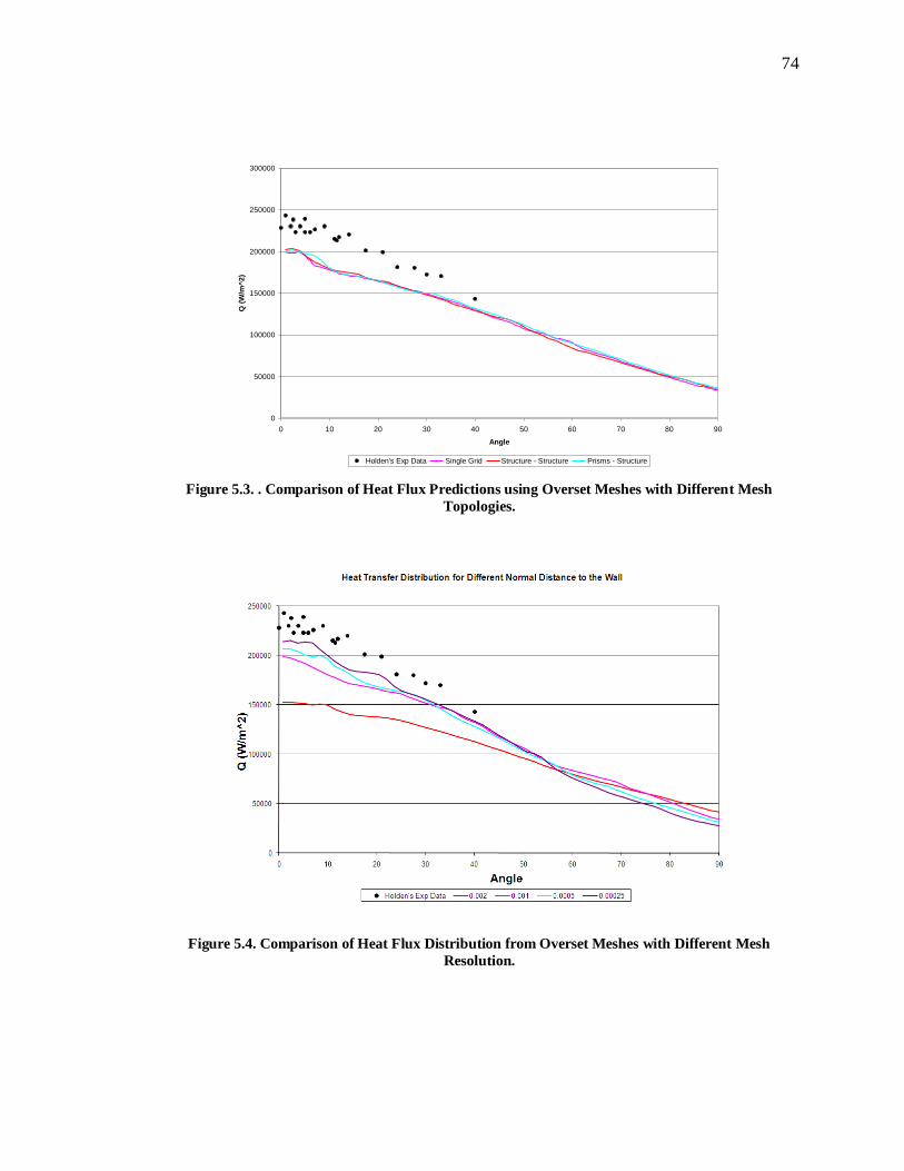
Figure 5.4. Comparison of Heat Flux Distribution from Overset Meshes with Different
Mesh Resolution. .................................................................................................................... 74
Figure 5.5. Temperature Contour for Cylinder Testcase with Single Mesh. ..................... 76
Figure 5.6. Cp Value at the Cylinder Surface. ..................................................................... 76
Figure 5.7. Heat Transfer at the Cylinder Surface. .............................................................. 77
Figure 5.8. Heat Transfer Contour at Cylinder Surface for Different Flux Schemes. ....... 77
Figure 5.9. Density Contour at Cylinder Surface for Different Flux Schemes. ................. 78
Figure 5.10. Pressure Contour at Cylinder Surface for Different Flux Schemes. .............. 78
Page 9
ix
TABLE OF CONTENT
ABSTRACT .............................................................................................................................ii
ACKNOLEDGEMENT .......................................................................................................... iv
LIST OF TABLES ................................................................................................................... v
LIST OF FIGURES ................................................................................................................ vi
1. INTRODUCTION ........................................................................................................... 1
2. LITERATURE REVIEW ................................................................................................ 5
2. 1. Hypersonic Flow ........................................................................................................... 5
2. 2. Hypersonic Simulation Challenges ............................................................................. 6
2. 2. 1. Stability of Numerical Scheme (Carbuncle Phenomenon) ................................. 7
2. 2. 2. Mesh Design, Quality, and Alignment .............................................................. 10
2. 3. Overset Mesh Benefits ............................................................................................... 11
2. 4. Hypersonic Experimental Tests and Ground Facilities ............................................ 14
3. NUMERICAL METHOD ............................................................................................. 16
3. 1. Governing Equations .................................................................................................. 16
3. 2. Riemann/Shock Tube Problem .................................................................................. 18
3. 2. 1. Roe Scheme ......................................................................................................... 21
3. 2. 2. HLL and HLLE scheme...................................................................................... 21
3. 2. 3. HLLC scheme...................................................................................................... 23
Page 10
x
3. 3. Adaptive Riemann Solver .......................................................................................... 25
3. 4. Higher Order Implementation and Limiter ............................................................... 27
4. NUMERICAL RESULTS ............................................................................................. 29
4. 1. Shock Tube Problem. ................................................................................................. 30
4. 2. Mesh Resolution Study for Shock-Tube Problem .................................................... 39
4. 3. 30o Supersonic Inviscid Ramp ................................................................................... 47
4. 4. Effect of Numerical Flux Evaluation on Solution Accuracy ................................... 52
4. 5. Overset Mesh Interpolation Study using Conserved and Primitive Variables. ...... 57
4. 6. Overset Mesh Study on a Hypersonic Cylinder........................................................ 58
4. 6. 1. Effect of Different Overset Mesh Interpolations on Solution Accuracy ......... 59
4. 6. 2. Effect of Different Overset Mesh Topologies on Solution Accuracy ............. 62
4. 6. 3. Effect of Different Overset Non-Dimensional Wall Distance on Solution
Accuracy .............................................................................................................. 63
4. 7. Shock/Shock Interaction in a Laminar Hypersonic Flow ........................................ 64
5. CONCLUSION AND FUTURE WORK ..................................................................... 70
5. 1. Future Work ................................................................................................................ 72
LIST OF REFERENCES ....................................................................................................... 79
Page 11
1
1. INTRODUCTION
A recent increase in space exploration has boosted interest in analyzing
hypersonic problems. Hypersonic technology is currently focused for developing space
vehicles with the purpose of space exploration. However, the future of hypersonic
technology is not limited just for space exploration, as globalization demands faster
public transportation. Flying with a hypersonic airplane at an average speed of Mach 5
allows people to travel from United States to Australia in just 2.5 hours compared to 14
hours required by the fastest commercial airplane currently available. The current
necessity was partially fulfilled by the commercial Concorde airplane which was capable
of cruising at a supersonic speed of Mach 2. The first hypersonic airplane intended to be
used inside the earth‟s atmosphere is the X-15 which has the capability to travel at a
maximum speed of Mach 6.7.
Hypersonic flow is characterized as a high temperature flow. The high
temperature is caused by extreme viscous dissipation within the boundary layer and also
by the temperature rise across the strong bow shock. The temperature at the nose region
of the Apollo reentry vehicle traveling at Mach 36 could reach up to 11,000 K[1]
. For this
reason, aerodynamic heat transfer study in hypersonic flows has become an important
subject for the development of reliable space vehicles. A reliable thermal protection
system (TPS) is required to prevent the space vehicle from melting.
Page 12
2
During the last decade, the computational fluid dynamic (CFD) technique has
matured enough to be routinely applied in the aerodynamic analysis of supersonic and
transonic problems. It is considered as an essential tool in the development of air
vehicles. However, a reliable prediction of aerodynamic heat transfer for hypersonic
problems still remains a challenge. Most of the shock capturing methods used for
transonic problems produce unrealistic solutions when used to solve hypersonic
problems[2]
. The unrealistic results are mostly caused by the numerical error which
dominates the physical solutions. The phenomenon is famously called as „carbuncle‟
phenomenon. Many cures have been developed for specific cases, but no universal cures
have been developed. The need for a universal cure for carbuncle is high and is still a big
challenge in the CFD field. A new adaptive scheme approach called HLLC+ was
introduced and believed to give accurate solution for hypersonic problems[3]
. More details
about the carbuncle behavior and several proposed cures will be elaborated in the
Literature Review chapter.
The first step in the CFD simulation process is mesh generation. The earliest
method developed for mesh generation is the structured mesh. In a structured mesh, the
domain of interest is decomposed into a number of quadrilaterals for two dimensions and
into hexahedrons for three dimensions. The next method developed is the unstructured
mesh where the domain of interest is divided into triangles for two dimensions and into
tetrahedrons for three dimensions. Both methods have their own strengths and
limitations. The structured mesh method is better in decomposing the boundary layer
region because of its capability to produce a good quality of high aspect ratio mesh.
Structured mesh method is computationally more efficient than the unstructured mesh
Page 13
3
method as the structured mesh method requires less data storage. The mesh connectivity
information in the structured mesh method is implicitly determined by the neighbor,
whereas, in an unstructured mesh method a data storage is required for all mesh
connectivity information. The unstructured mesh however is superior to the structured
mesh for complex geometry problems and mesh adaptation approaches. The time
required to generate an unstructured mesh for complex geometry is less than that for a
structured mesh.
In an attempt to combine the advantages of both the structured and unstructured
mesh method, a new meshing method called the generalized mesh has been developed[4]
.
Generalized mesh is an unstructured mesh composed of arbitrary polyhedrals. It allows
the flexibility to generate various mesh shapes. Therefore, it provides the possibility to
create high aspect ratio meshes at boundary layer region. The generalized mesh method
however still faces difficulty when used for moving body or large deformation
problems[5],[6],[7]
. The method will generate skewed meshes in the moving-body or large
deformation region. For moving body and large deformation problems, an overset mesh
method is considered to be the best approach. An overset mesh method is a method of
using more than one mesh to decompose the domain of interest. The meshes are
overlapped with each other and are solved separately. An interpolation approach is used
to transfer appropriate flow variables between the meshes. By using the overset mesh
approach the domain of interest and the environment could be represented in difference
meshes which could avoid the generation of skewed meshes.
Another common difficulty in simulating complex fluid flow problems is that not
all geometries can be well represented with a single mesh. In many cases, different
Page 14
4
geometrical features are best represented by different mesh types. The overset mesh
approach helps to solve these difficulties by constructing a mesh system made of
overlapping meshes. The complex fluid problem is decomposed into much simpler
overlapping meshes and the time required to generate each mesh is reduced. The
summary of benefits and limitations for each mesh type are presented in Table 1.1.
The objectives of this research are: 1) to evaluate different convective fluxes in
laminar hypersonic problems; 2) to implement a new adaptive scheme, HLLC+,
introduced by Trammel, R. et.al.[3]
in our generalized mesh based CFD solver, HYB3D[4]
;
3) to study the error estimation of heat transfer using the overset mesh method with three
different parameters: different interpolation methods, different mesh topologies, and
different non-dimensional wall distance.
The thesis is constructed as follows: Chapter one covers the introduction and
background. Chapter two covers a brief summary of hypersonic flows and its challenges.
Chapter three describes the numerical schemes for the solution of the governing
equations. Chapter four discusses the results. Chapter five covers the conclusion and
future work.
Table 1.1. Advantages and Disadvantages of Four Meshing Methods.
Structured Unstructured Generalized Overset
Complex Geometry - + + +
Mesh Adaptation - + + +
Mesh Generation Time - + + +
Memory Requirement + - - -
Solver Time + - - -
Viscous Computation + - + +
Moving Body Problems - - - +
Page 15
5
2. LITERATURE REVIEW
This section briefly talks about hypersonic flow and the difficulty in achieving
accurate prediction in computer simulation. The attempt to get a better hypersonic
prediction and a cure for the carbuncle phenomenon is covered in this chapter. The
introduction and the potential benefit of the overset mesh approach are also explained.
2. 1. Hypersonic Flow
Hypersonic flow is a flow which travels at a velocity that exceeds Mach 5.
However, some flows under Mach 5 could produce a characteristic similar to hypersonic
flow. The dividing line between supersonic to hypersonic flows is not as obvious as from
subsonic to supersonic flow. According to J.D. Anderson, the best interpretation of
hypersonic flow is a flow region where the flow phenomena become gradually more
important as the Mach number increases[1]
. Another indicator of hypersonic flow is that it
is characterized by much smaller internal thermodynamic energy than kinetic energy[1]
.
Hypersonic flow is also characterized as a high temperature flow. The high temperature is
caused by extreme viscous dissipation within the viscous boundary layer of the
hypersonic flow. In the early 1950s, H. Julian Allen of Ames Aeronautical Laboratory
came up with a blunt body design that allows a shock layer region to be created in front
of the nose region, to deflect most of the heat away from the vehicle[8]
. Even with the
Page 16
6
blunt body design, the temperature at the shock layer region of the Apollo during reentry
at Mach 36 actually reached up to 11,000 K[1]
. Therefore, in order to design reliable
hypersonic vehicles, the study of the heat transfer for a hypersonic flow environment is
very crucial. Current re-entry vehicles use ablative materials for thermal protection
systems. The ablative materials help in transferring the generated heat away from the
vehicle, which results in a decrease in temperature at the surface of the re-entry vehicle.
The cost to run a space vehicle prototype in ground experiments is very expensive. Also,
there is difficulty in generating exact outer space environment in ground experiments.
Knowing the limitations and high cost of conducting ground experiments, an alternative
approach is needed to validate the design of hypersonic vehicles. Computer simulation
approach has already been used in many airplane designs and proven to give reliable
solutions. Thus, using computer simulation to predict the heat transfer in hypersonic flow
has become a viable alternative for designing and developing hypersonic vehicles.
2. 2. Hypersonic Simulation Challenges
Even with the maturity of computer simulation for subsonic and supersonic
problems, simulating a high-quality hypersonic flow is still a challenging task to
accomplish[9],[10]
. One of the most challenging tasks in hypersonic simulations is to
calculate an accurate aerodynamics heat transfer[11],[12]
. The complexity of the chemical
reaction and the transport phenomena is difficult to model which leads to inaccurate
prediction on the heat generated from chemical reactions. Another common challenge is
to select an accurate and stable numerical scheme to calculate the solution in hypersonic
flows. Most of the high fidelity shock-capturing methods used for subsonic and
Page 17
7
supersonic problems suffer from the well-known phenomena called „carbuncle‟ when
used for hypersonic problems[2]
. In order to get high-quality prediction of aerodynamic
heating, several parameters need to be carefully selected such as: stability and order of
accuracy of the scheme used, and mesh design, quality, and alignment to the shock.
2. 2. 1. Stability of Numerical Scheme (Carbuncle Phenomenon)
The most commonly used shock capturing method for subsonic and supersonic
problems is the flux difference splitting scheme also known as the Riemann solver.
However, the scheme faces challenges in producing reliable solutions when used to solve
hypersonic problems. The pathological behavior was first reported by Peery and Imlay in
1988, during simulations on high speed flows over a cylinder[13]
. The pathological
behavior is also known as a carbuncle phenomenon and the cause is still not completely
understood. It is believed that carbuncle is a phenomenon that occurs when the numerical
error in the stagnation region dominates the real physical solution and leads to spurious
unphysical solution[14]
.
Pandolfi[5]
categorized the Flux Difference Splitting method into three types
(Figure 2.1): 1) a strong carbuncle prone scheme where pressure perturbations damp out
while creating constant density perturbations. 2) A light carbuncle prone scheme where
pressure perturbations remain constant and do not interact with the constant density
perturbations. 3) A carbuncle-free scheme where density perturbations damp out with or
without mutual interaction with pressure perturbations.
Page 18
8
a) Carbuncle Prone. b) Light Carbuncle. c) Carbuncle Free
Figure 2.1. Types of Flux Splitting Schemes.
Liou[15]
hypothesized that the pressure term of a governing equation causes the
instability and initializes the numerical error. He stated that in order to cure the
instability, the pressure term has to be separated from the governing equation. However,
this method is considered non-physical because the pressure also affects the mass balance
of the governing equation[16]
. In addition this scheme still suffers from carbuncle.
Ismail[16]
hypothesized that carbuncle is divided into three different states: pimple,
bleeding, and carbuncle. At the pimple state, the spurious vorticity starts being produced
along the shock. Depending on the Mach number, the pimple stage may or may not last
long and will develop into the bleeding stage. In the bleeding stage, the spurious result
starts to take effect downstream of the shock. The bleeding stage is most visible in the
Mach number, velocity, and vorticity contours. The last stage is the carbuncle where the
spurious solution dominates all the upstream and downstream conditions of the shock.
The behavior is in agreement with flux analysis performed by Dumbser[17]
. In his
research, he observed that the instability begins in the upstream region and influences the
Page 19
9
downstream solution, which explains why the shock-fitting scheme never produces
instability on a blunt body problem. Ismail[16]
suggests that in order to cure the carbuncle,
a scheme has to prevent the creation of the pimple stage. He proposed the use of vorticity
control method to prevent this phenomenon.
Both Loh[18],[19]
and Xu[20],[21]
agreed that the amount of dissipation at the cell face
tangential to a shock is much less or closer to absent than the dissipation at a normal cell
face. The tangential cell face at A-B and C-D in Figure 2.2 has a very small pressure
gradient between its left and right cells. However, the normal cell face A-C and B-D has
very large pressure gradients because of the shock properties. They concluded that the
Riemann solver does not produce enough dissipation at the tangential faces to the shock;
adding numerical dissipation to these faces will provide greater stability. These results
are also agreed by Henderson[22]
, who studied different tangential face angles and found
that the angle with less than a 90 degree tangential face will produce fewer carbuncles.
Figure 2.2. Shock Dissipation at Cells Differs at Tangential Face (A-B, C-D) and at Normal Face (A-
C, B-D).
Kitamura[23]
investigated several methods that suffer from carbuncle and
hypothesized that carbuncle is not only a one-dimensional but a multidimensional
problem. He found that some schemes that were not stable in one dimension would also
Page 20
10
fail in multidimensional problems. He believed that multidimensional dissipation is
needed to cure the instability.
Many fixes for the Riemann Solver have been proposed in the last decade but
these fixes only work for specific problems, and no universal cure has been agreed upon.
Greater understanding of the carbuncle is still being investigated. Two major approaches
to cure Riemann solver from the phenomenon are: 1) Adding a numerical dissipation
directly to the convective flux calculation part. 2) Using a combination of high and less
dissipative schemes by introducing a switching parameter to switch between those
schemes. From these two approaches, it is agreed that adding more dissipation to the
convective part of the numerical scheme could suppress the phenomenon. The drawback
of using a high dissipation scheme is that it will reduce the order of accuracy of the
numerical scheme being used.
2. 2. 2. Mesh Design, Quality, and Alignment
In order to have an accurate heat transfer prediction, only preventing the
occurrence of carbuncle is not enough. Mesh design, mesh quality, and mesh alignment
are also very important factors for solving accurate heat transfer in hypersonic flow.
Detailed mesh study for inviscid and viscous hypersonic flows have been performed by
Henderson[22]
. The effect of the mesh aspect ratio, mesh clustering at the shock location,
mesh alignment with the shock structure, and mesh size were studied. Different mesh
aspect ratios were studied and the result indicated that the carbuncle was greatly reduced
as the aspect ratio increased, as shown in Figure 2.3. The result is in agreement with the
finding by Pandolfi[2]
. Mesh clustering at the shock location to increase the mesh aspect
Page 21
11
ratio has also proven to reduce the carbuncle effect. In order to do mesh clustering, an
adaptive mesh capability is needed. Xu and Hu also believe that the numerical dissipation
at a cell face is dependent on the orientation of the shock[24]
. The more perpendicular a
cell face is to the shock, the less numerical dissipation is being produced. No dissipation
is produced if a cell face is laid exactly perpendicular to the shock. The same conclusion
was also given by Henderson[22]
. Henderson also concluded that the mesh misalignment
with the shock will produce a greater magnitude of carbuncle, caused by less dissipation
when the mesh is misaligned with the shock location.
The effect of mesh design and topology were studied by Gnoffo[10],[11]
who
concluded that a tetrahedral mesh with mesh alignment to the shock still produces
spurious solutions. It is suspected that using a tetrahedral mesh will create uncontrollable
mesh misalignment and cause the spurious solution. The study using a tetrahedral mesh
was also conducted by Candler[12]
who also concluded the same results.
a) Low aspect ratio cell produces
more carbuncle.
b) High aspect ratio cell produces
less carbuncle.
Figure 2.3. Effect of Cell Aspect Ratio and Carbuncle.
2. 3. Overset Mesh Benefits
Overset mesh is a method that uses a set of overlapping meshes to discretize the
domain of interest. The overset mesh method has already been used for more than twenty
years to simplify the mesh generation process. The method is also known as Chimera
mesh[7]
. One of the benefits of using the overset mesh method is that it significantly
Page 22
12
reduces the mesh generation time, especially for complex geometries. In the process of
design optimization, design changes occur rapidly. When using the overset mesh method,
only the parts that are re-designed need to be re-meshed. Thus, the whole design does not
need to be created repeatedly which could save a significant amount of mesh generation
time. For example, in the shuttle wing design process, there is no need to create a whole
new shuttle mesh every time the wing design is changed. The overset mesh method gives
the capability to add only the new wing design mesh to the entire overset mesh. The other
benefit of overset mesh is that it can be used effectively to perform large body
deformations or moving body simulations. By using the overset mesh method, the need to
regenerate the mesh for every time step is not required. One example of a moving body
simulation which could use the overset mesh method is the store separation simulation.
The development of overset meshes for structured meshes is already in a mature state and
is used for many applications, with the application of overset mesh for unstructured and
generalized overset meshes rapidly following[10]
. This makes the study using the overset
mesh method for unstructured and generalized meshes very promising.
The most important step in using overset mesh method is to connect the solution
between each mesh. The overlapping meshes in the overset method are connected by
appropriate interpolating points between all the meshes. These points are called fringe
points. The fringe points that will provide the information to the other vicinity meshes are
called donor points. The points that collect the information from the donor are called
receptor points. The domain that wants to be excluded from being calculated in order to
save computational time is marked as hole points or blank regions. If the receptor points
do not have valid donor members, then the area will be marked as orphan points. All this
Page 23
13
important point information is collected in a database called the domain connectivity
information. Domain connectivity information also includes the information about the
corresponding fringe points for each donor and receptor point. A close look at an overset
mesh assembly is shown in Figure 2.4. Two individual meshes are used, a body-fitted
cylinder mesh and a background mesh. The recipient fringe points for the body-fitted
cylinder mesh are colored with black dots. The values at these fringe points are calculated
by interpolating the value from the neighboring cells of the background mesh. The
cylinder fringe points act as a boundary value for the cylinder mesh. The similar
interpolations also happen with the background recipient fringe points. The green dots
represent the hole cutting or blank region of the background mesh, where no
computational calculation is executed to reduce the computational cost.
a) Overset assembly b) Close-up view of overset assembly
Figure 2.4. Overset Mesh Method Assembly.
Page 24
14
Most of the legacy computational fluid dynamic solvers are not developed for the
overset mesh method. However, the overset capability can be added by appropriate
modifications to the CFD solvers. A software called SUGGAR (Structured, Unstructured
and Generalized overset Grid AssembleR) has been created by Noack[25]
to assemble an
overset mesh from single meshes and also to create all the domain connectivity
information. The overset mesh generation using SUGGAR is highly automated. Software
called DirtLib (Donor interpolation Receptor Transaction Library) has also been
developed by Noack[26]
. This software envelops all the routine requirements for the
overset mesh method into a general CFD solver and performs the overset mesh
interpolation to the appropriate location. With the benefit of these two algorithms, an
overset mesh assembly can be performed automatically using a single mesh flow solver.
2. 4. Hypersonic Experimental Tests and Ground Facilities
Milner[27]
had collected hypersonic experimental data from the past decade. Flight
experiment is very costly and not much data is available for hypersonic flight tests. Most
of the hypersonic experimental data is taken from ground tests inside a wind tunnel. The
experimental data that are often used for comparison with the simulation result is
acquired from the ground test data, not from the flight test. The most commonly used
experimental data for computational benchmark is the hypersonic flow over a cylinder.
The test case is commonly chosen because of the simplicity of the geometry and the
accuracy of wind tunnel experimental data.
Several groups had performed experimental benchmark cases for hypersonic heat
transfer. Calspan University at Buffalo research center (CUBRC) and Office National
Page 25
15
d'Études et de Recherches Aérospatiales (ONERA) are among the leaders in performing
hypersonic ground experiments for generating benchmark data in their wind tunnels. At
CUBRC, the supersonic and hypersonic flows are tested at Large Energy National Shock
Tunnel facilities (LENS). The facilities have been used for solving aerodynamics
problems including planetary reentry to Earth and Mars. At ONERA, the fundamental
studies are mostly performed in the R5Ch wind tunnel. The R5Ch wind tunnel has also
been used as a benchmark for some of the advanced experiments performed in other wind
tunnels. The benchmark data used in this study were obtained from experimental test
cases performed at CUBRC and ONERA.
NATO Research and Technology Organization Advanced Vehicle Technology
(RTO-AVT) collected most of the ground test experimental data. For this purpose, they
started a panel called “Working Group 10 (WG 10)”. The collected data is very useful for
comparing the accuracy of the numerical scheme.
Page 26
16
3. NUMERICAL METHOD
Upwind scheme is one of the most commonly used numerical schemes for
subsonic and supersonic problems that deal with shock. However, the scheme suffers
from spurious solution when used for hypersonic problems. The purpose of this study is
to analyze the adaptive scheme of Roe-HLLE and HLLC+ to prevent this spurious
solution. This chapter describes: 1) the discretization of the equations governing fluid
flows using a finite volume approach, 2) a brief introduction and explanation about
Riemann problems and Riemann solvers, and 3) the evaluation and the implementation of
convective fluxes using the HLLC+ scheme.
3. 1. Governing Equations
The governing equations for a computational fluid dynamics solver are based on
three fundamental physical principles: conservation of mass, conservation of momentum,
and conservation of energy. These equations can be written in either differential or
integral form. The integral form of the governing equations is preferable for solving a
fluid flow problem using unstructured mesh because the form allows the use of any
elements with an arbitrary number of faces. The integral form of the governing equation
can be written as:
Page 27
17
s
v
v
dsnFdsnFdvQdt
d
(3.1)
Where: n
is the unit vector pointing outward from the control surface, is the control
volume, and ds is the control surface area.
The conserved variable vector n
Q
is defined as
E
w
v
u
.
The inviscid flux vector nF
is defined as
t
z
y
x
pnpE
pnw
pnv
pnu
.
The viscous flux vector nF v is defined as
zzyyxx
vvv
zzzyyzxxz
zyzyyyxxy
zxzyxyxxx
v
v
v
v
v
nTnTnTkwfvfuf
nnn
nnn
nnn
f
f
f
f
f
4325
4
3
2
10
.
nt is the contravariant velocity component of the grid speed and is defined as follows:
ztytxtt nznynxn ; β is the contravariant velocity component of the fluid particle with
respect to the grid and is defined as tn ; where zyx wnvnun , and E is the
total energy per unit volume and is defined as 222
2
1
1wvu
pE
.
The discretized form of the governing equation can be written as[28]
:
Page 28
18
mn
o
n
GCLo
n
o
n
o
n
o
n
o
mn
o
n
o
mn
i
i
mn
omn
o
o
mn
o
n
o
RHSRHSQt
QVQQV
QQ
RHSQ
Q
RHS
t
IV
,11
,
11
2
,11
2
,1,1
,1,11
2
1
1
where V is the volume of the cell, the subscript i represents all the neighboring cells that
surround the reference cell o, where θ2 is the parameter for the selection of the time order
of accuracy and 2=0 for first order time and 2=1/2 for second order time, superscripts n
and n+1 represent the times steps, superscript m represents the Newton iteration level,
RHS0 is the summation of inviscid and viscous fluxes, and RHS0,GCL is the flux resulting
from mesh deformation.
The discretization of the governing equation described above, has been
implemented in a parallel framework for generalized meshes. A CFD solver based on the
generalized meshes framework, known as HYB3D, has been developed. The solver has
been validated with different benchmark testcases[5],[6]
. The framework will be used for
the implementation of new flux evaluation schemes.
3. 2. Riemann/Shock Tube Problem
Shock-tube problems are the main foundation of the flux difference scheme. In
order to understand the mechanism of flux difference splitting scheme, the shock-tube
problems need to be understood. Shock-tube problem is a fundamental tool used to study
the interaction between waves. It is very beneficial in understanding the hyperbolic
partial differential equation such as the Euler equation. Shock-tube problem also gives an
Page 29
19
exact solution to some complex nonlinear equations which are useful as the benchmark
test for numerical schemes study.
The initial condition of the shock-tube problems is composed of two uniform
states separated by a discontinuity membrane, as shown in Figure 3.1.a. The pressure on
one side of the membrane is greater than the other side (PL > P R). All viscous effects are
negligible along the tube walls and the tube is assumed to be infinitely long in order to
avoid reflections at the tube end. When the discontinuity membrane is instantaneously
removed, the pressure discontinuity propagates to the lower pressure region.
Simultaneously as the membrane is removed, the discontinuity breaks into two leftward
and rightward moving waves separated by a contact discontinuity wave and creates four
different regions in the shock-tube, as shown in Figure 3.1.b. The shock divides region
one and two which have the discontinuity for density, pressure, and velocity. Region two
and three are separated by a contact discontinuity which have a discontinuity in density,
but have constant pressure and velocity. In the rarefaction wave region, the fluid
properties smoothly change from region three to region four. The solution of the flow
field in the shock tube is sketched in Figure 3.1. The shock-tube problem is also known
as the Riemann Problem.
a) Initial Condition of The Shock Tube Problem.
Page 30
20
b) Condition After The Membrane is Removed at Time t.
Figure 3.1. Shock-tube Problem.
The nature of the finite volume method can be represented as a series of Riemann
problems. The value at mesh point i at time level t can be calculated as an average of the
properties created by the waves coming from the left and right sides as shown in Figure
3.2. The philosophy of shock-tube problems initiates the birth of exact and approximate
Riemann solvers. The exact Riemann solver, also known as the Godunov Method, finds
the exact solution of the Riemann problem by considering the speed, direction, and
strength of discrete pressure waves, shock waves, and contact discontinuity waves
emerging from the cell interface. The exact Riemann solver is more iterative and
computationally more expensive than the approximate Riemann solver. The approximate
Riemann solver uses approximate solutions to solve the Riemann problem which
significantly reduces computational cost. Because of this benefit, the study will use
approximate Riemann solvers. Examples of commonly used Riemann solvers are the
Roe, HLLC, and HLLE schemes.
Page 31
21
Figure 3.2. Riemann Problems at Each Interface.
3. 2. 1. Roe Scheme
The Roe scheme is the most popular and most widely used approximate Riemann
solver because of its accuracy and robustness. The scheme however suffers from the
carbuncle phenomenon when used for solving hypersonic problems due to the fact that it
captures the contact discontinuity. The assumptions and theory of the Roe scheme[34]
are
not included in this work. The Roe flux through a cell face is calculated as:
)(||)()(
2
1 _
RLRLRoe QQAQFQFF
(3.5)
Where 1 TTA . T is a matrix whose columns are the right eigenvectors of A ,
T-1
is a matrix with its rows as the left eigenvectors of A , and is a diagonal matrix
whose elements are the absolute values of the eigenvalues of A .
3. 2. 2. HLL and HLLE scheme
Harten, Lax, and van Leer proposed a novel approach for solving a Riemann
problem which later became known as the HLL scheme. This approach obtains the
approximation for the inter cells numerical flux directly. The scheme assumed that two
Page 32
22
waves, with speed of SL and SR, separate three constant values. SL and SR are the fastest
signal velocities and are assumed to be known. The conserved variables of the HLL
scheme are given as:
.0
,0)()(
,0
RR
RLLR
RRRLLLM
LR
HLL
SifQ
SSifSS
QSFQSFQ
SifQ
Q (3.6)
The Rankine-Hugoniot jump conditions across the left and right waves are used to
find flux variable FM, which are )( LMLLM QQSFF and )( RMRRM QQSFF
and the final expression of the flux variables is:
)( LRLR
LR
LR
RLLRM QQ
SS
SS
SS
FSFSF
(3.7)
0
0
0
RR
RLM
LL
HLL
SifF
SSifF
SifF
F (3.8)
Figure 3.3. One Intermediate State of HLL and HLLE Riemann Fan.
While the HLL scheme is very efficient and robust, the two waves assumption is
only accurate for hyperbolic systems of two equations, as shown in Figure 3.3.
Determining the wave speeds is very crucial to have stable and not overly dissipative
Page 33
23
solutions when using the HLL scheme. To stabilize the scheme, Einfeldt et al[36]
proposed
a way to determine the wave speed as follow:
LL auauS )(,~~,0min (3.9)
RR auauS )(,~~,0max (3.10)
Where u~ and a~ are the Roe-averaged properties and speed of sound value respectively.
The HLL scheme that uses the wave speed criteria as Einfeldt et al[36]
proposed is better
known as the HLLE scheme. The use of the wave speed helps to ensure the method to be
positively conservative and prevent the HLLE scheme from generating a vacuum state,
which makes it more stable than the original HLL scheme. Because the HLLE scheme
does not take the contact discontinuity into account, the scheme does not suffer from the
carbuncle phenomenon. However the scheme is known to have excessive dissipation at
the boundary layers.
3. 2. 3. HLLC scheme
The HLLC scheme, where C stands for Contact Wave, tries to restore the missing
contact discontinuity and shear waves which the HLL scheme ignore. The contact
discontinuity waves speed is represented by SM and is calculated as
)()(
)()(
LLLRRR
LRRRRRLLLLM
uSuS
PPuSuuSuS
(3.11)
Where )a),(uauS LL )~~((min and ))(),~~max(( RR auauS .
In the HLLC scheme the intermediate state is divided into two separate regions, as shown
in Figure 3.4. The integration over the control volume for these regions gives two integral
averages Q*L and Q*
R and the relation of these values with QM can be found using the
HLL scheme.
Page 34
24
**R
LR
MRL
LR
LMM Q
SS
SSQ
SS
SSQ
(3.12)
The Rankine-Hugoniot jump condition is used across each wave speed (SL, SM, SR). With
the fact that the pressure and velocity component normal to the contact waves are
constant, the intermediate state of conserved variable and fluxes values are solved
(equations 3.9 – 3.10). The Rankine-Hugoniot jump conditions are:
)( **LLLLL QQSFF , )( ****
LRMLR QQSFF , and )( **RRRRR QQSFF
Figure 3.4. Two Intermediate States of The HLLC Riemann Fan.
)()(
)(
)(
)(
*
KKK
KMKMK
zMK
yMK
xMK
MK
KKL
K
qS
PSqSE
qSw
qSv
qSu
SS
qS
Q
K
K
K
(3.13)
Where K = L or K = R
0
0)(
0)(
0
**
**
RR
RMRRRRR
MLLLLLL
LL
HLLC
SifF
SSifQQSFF
SSifQQSFF
SifF
F (3.14)
Page 35
25
The HLLC scheme offers more accurate and less dissipative predictions at the
boundary layers than the HLL/HLLE scheme. However, the scheme is vulnerable to the
carbuncle phenomenon because it captures the contact discontinuity exactly.
3. 3. Adaptive Riemann Solver
Many numerical schemes have been proposed in the literature to combine
different numerical schemes to avoid carbuncle phenomenon and to get better accurate
results. This class of schemes is called adaptive schemes. One of the adaptive schemes
that is present in the current numerical framework is the adaptive Roe-HLLE scheme.
One of the methods to cure the carbuncle phenomenon is by using a combination
of Riemann solver. A dissipative Riemann solver does not suffer from the phenomenon.
However, a Riemann solver has to have just enough dissipation to calculate the prediction
of shock location and viscous boundary layer accurately. The idea of using a switching
Riemann Solver was proposed by Quirk[14]
in 1992. He suggested using a combination of
a high and low dissipation Riemann Solver to prevent the shock instability and to have
the ability in capturing the shock location exactly. He proposed the idea of using a
pressure parameter to specify a strong shock region. The switching parameter is based on
a pressure jump between the reference cell and its neighbors and is defined as,
),min(
||
RL
LR
pp
pp , where = threshold parameter (3.15)
The threshold parameter is problem dependant and can be adjusted according to
how much dissipation is needed. Quirk[14]
chose to switch between the Roe and HLLE
methods. Roe scheme was used in no strong shock region and HLLE scheme was used
when the condition of Equation 3.15 was satisfied. Even though the HLLE scheme is
Page 36
26
believed to be very dissipative, the use of this scheme in the vicinity of a strong shock
will not reduce the total scheme accuracy. The use of the Roe-HLLE adaptive scheme
gives smoother and more realistic conserved variables contour than using Roe or HLLE
scheme alone.
Another adaptive scheme method was proposed by Trammel et al.[3]
which used
the combination of HLLC and HLLE Riemann solvers. The approach is called the
HLLC+ approach. The idea of using an adaptive scheme is to have an accurate solution
without the need of generating shock-alignment mesh. The performance of the HLLC+
approach gives a better solution than the original HLLC or HLLE scheme and also
maintains the time accuracy[3]
. The implementation of the HLLC+ flux calculation for
generalized mesh is:
HLLEHLLCHLLCHLLC FFF )1( (3.16)
)4.0,max( NewHLLC (3.17)
otherwise
DeltaSif
p
w
New)10tanh(1
/0.10.0
3 (3.18)
)0,/max( DeltaSwp (3.19)
),max( RLw kkS (3.20)
),min(
||
RL
LR
pp
ppk
(3.21)
The Delta value of 1 to 10 has been found to be adequate to eliminate the
carbuncles and errors induced when strong shocks are present. FHLLC and FHLLE are
calculated using the flux calculation of HLLC and HLLE scheme respectively. The value
of βHLLC+ is used to limit the high dissipation produced by HLLE. βNEW is the switching
Page 37
27
parameter. k is the pressure switch sensor and it is in first order accurate. The original
HLLC+ formulation is generated for structure mesh solver and the pressure switch is
based on the second derivative of pressure, while the current implementation is based on
the first derivative of pressure.
The HLLC+ scheme is implemented for a generalized mesh framework and the
results from the validation of the scheme is given in the next chapter. Both adaptive
scheme Roe-HLLE and HLLC+ will be used in this study to validate the overset mesh
methodology.
3. 4. Higher Order Implementation and Limiter
In order to have a better solution representation, second order linear
reconstruction from the cell averaged values is applied. The piecewise linear
reconstruction of the conserved variables from the cell averaged values is calculated
using the Taylor‟s series expansion from all the neighboring cells. During the solution
process, the values at the cell face are extrapolated using the cell averaged values.
The practice of getting a high order solution by adding the gradient of flow
variables could produce local minima and local maxima. The creation of local minima or
local maxima will induce a high chance of creating spurious oscillations of the flow
variables near regions of the high solution gradient. The limiter function is used to
prevent the development of the spurious oscillations and also to preserve the
monotonicity. The limiter function is applied directly to the gradient of the flow variables
in the Taylor‟s series expansion. The disadvantage of using the limiter function is that it
will reduce the order of accuracy of the scheme used in those regions. The limiter used in
Page 38
28
this study is the limiter function introduced by Barth[29]
. The limiter condition is shown in
equations 3.22 and 3.23. QL is the neighboring cell and QC is the value at the cell center.
)min( FBarth (3.22)
01
0,1min
0,1min
min
max
CL
CLCL
CL
CLCL
CL
F
QQif
QQifQQ
QQ
QQifQQ
QQ
(3.23)
where ),min(min
nCcell QQQ and ),max(max
nCcell QQQ
Page 39
29
4. NUMERICAL RESULTS
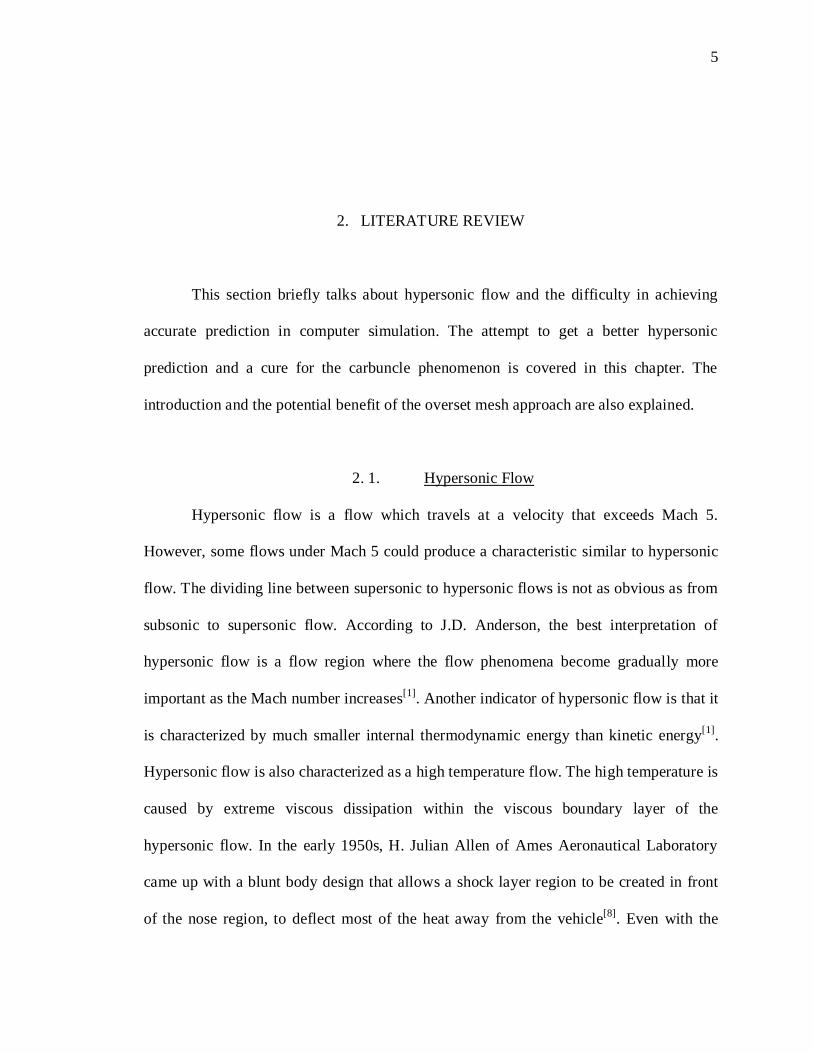
The carbuncle phenomenon occurs when a Riemann solver tries to capture the
contact discontinuity exactly. An example of carbuncle phenomenon is shown in Figure
4.1. The numerical error dominates the physical solution which creates an unphysical and
spurious solution. In order to prevent the carbuncle phenomenon, two types of adaptive
scheme fixes were investigated: the adaptive Roe – HLLE and HLLC+. Laminar
hypersonic flows of calorically and thermally perfect gases without chemical reaction
were used for investigating the accuracy of these numerical schemes.
a) Mesh used for Hypersonic
Cylinder testcase.
b) Carbuncle
Phenomenon
Figure 4.1. Carbuncle Phenomenon for Flow over a Hypersonic Cylinder.
Page 40
30
4. 1. Shock Tube Problem.
To validate the implementation of HLLC, HLLE, and HLLC+ schemes for the
solution of the Riemann problem, shock tube problems with different initial conditions
were used. Toro[30]
provides several initial value problems to investigate the accuracy and
robustness of a Riemann solver. These initial conditions are tabulated in Table 4.1, where
Xo is the location of the initial discontinuity. The spatial domain of the shock tube
problem is taken as 0 ≤ x ≤ 1. The numerical solution is computed with a three
dimensional structured mesh of dimension 100 x 10 x 10 in x, y, and z directions
respectively. A CFL number of 0.9 and the specific gas constant of 1.4 are used for these
simulations.
Table 4.1. Initial Condition for Shock Tube Problems.
Test ρ L u L P L ρ R uR P R Xo
1 1.0 0.75 1.0 0.125 0.0 0.1 0.3
2 1.0 -2.0 0.4 1.0 2.0 0.4 0.5
3 1.0 0.0 1000.0 1.0 0.0 0.01 0.5
4 5.99924 19.5975 460.894 5.99242 -6.19633 46.0950 0.4
5 1.0 -19.59745 1000.0 1.0 -19.5975 0.01 0.8
Test 1 has a shock wave and contact discontinuity traveling to the right and
rarefaction waves traveling to the left. The test is useful in assessing the entropy
satisfaction property of numerical methods. Test 2 is suitable for assessing the
performance of numerical methods for low-density flows. Test 3 has a strong shock and
is designed to assess the robustness and accuracy of numerical methods. Test 4 has three
different discontinuities moving to the right and is also designed to assess the ability of
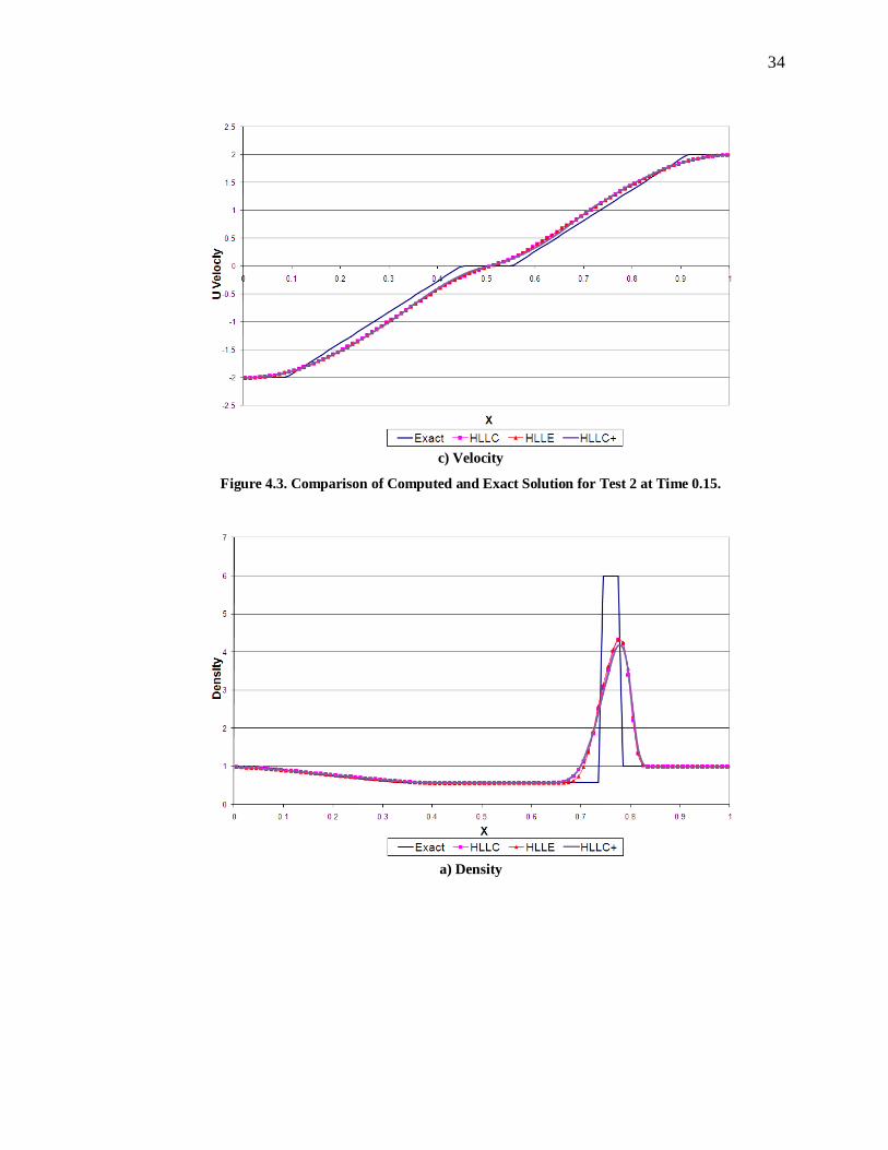
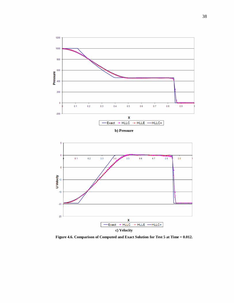
the numerical methods to resolve slow moving contact discontinuity. Test 5 consists of
rarefaction waves traveling to the left and shock traveling to the right with a stationary
contact discontinuity. The comparison of the numerical results with the exact results for
Page 41
31
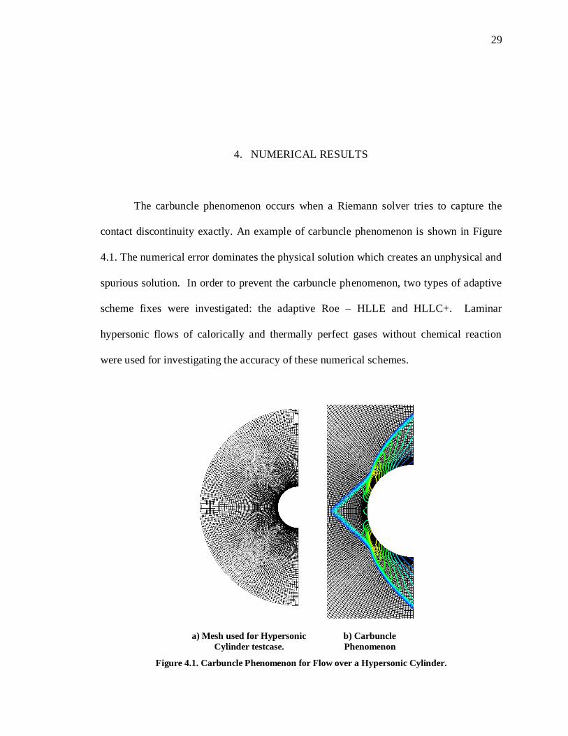
these five shock tube problems are shown in figure 4.2 – 4.6. It can be seen from these
figures that HLLC, HLLE, and HLLC+ with the value Delta of 5 predicts the results
accurately.
As shown in Figure 4.2, HLLC+ and HLLE scheme predict a better velocity
profile at the shock discontinuity than HLLC scheme for test 1. In test 2 and test 3, Figure
4.3 and Figure 4.4, all three schemes give similar solutions. For test 4, Figure 4.5 the
HLLC+ scheme gives a better shock discontinuity prediction than the other two schemes.
Also in test 5, Figure 4.6 the HLLC+ gives more accurate value in locating the shock
discontinuity than HLLC or HLLE.
a) Density
Page 42
32
b) Pressure
c) Velocity
Figure 4.2. Comparison of Computed and Exact Solution for Test 1 at Time 0.2.
Page 43
33
a) Density
b) Pressure
Page 44
34
c) Velocity
Figure 4.3. Comparison of Computed and Exact Solution for Test 2 at Time 0.15.
a) Density
Page 45
35
b) Pressure
c) Velocity
Figure 4.4. Comparison of Computed and Exact Solution for Test 3 at Time 0.012.
Page 46
36
a) Density
b) Pressure
Page 47
37
c) Velocity
Figure 4.5. Comparison of Computed and Exact Solution for Test 4 at Time 0.035.
a) Density
Page 48
38
b) Pressure
c) Velocity
Figure 4.6. Comparison of Computed and Exact Solution for Test 5 at Time = 0.012.
Page 49
39
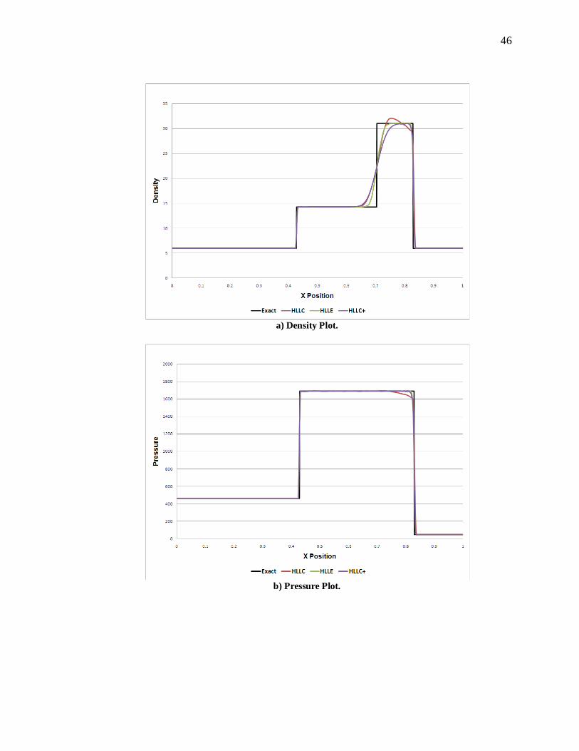
4. 2. Mesh Resolution Study for Shock-Tube Problem
A study of effect of mesh resolution to the solution of shock tube problem has
been performed. In this study shock-tube problem 4 has been selected as the benchmark
case because it has the strongest shock and a slow moving contact discontinuity. Another
reason for selecting this testcase for the mesh resolution study is that the numerical
results from all other four cases behaved similarly with the exact solution as compared to
test 4. Three different meshes of sizes 100x10x10, 200x10x10, and 400x10x10 are used
for this study. The results from the study are presented in Figure 4.7 to Figure 4.12 for
HLLC, HLLE, and HLLC+. In general, as the mesh resolution increases the contact
discontinuity and the shockwave are predicted with better accuracy. From Figure 4.7 to
Figure 4.12, it can be seen that HLLE scheme gives the smoothest density, pressure, and
velocity contours while the HLLC scheme gives the most spurious contours. The HLLE
scheme also gives the best prediction of shock and contact discontinuity locations with
the lowest dissipation.
a) Density Contour
Page 50
40
b) Pressure Contour
c) Velocity Contour
Figure 4.7. Results from Mesh Resolution Study using HLLC scheme.
a) Density Contour.
Page 51
41
b) Pressure Contour.
c) Velocity Contour.
Figure 4.8. Results from Mesh Resolution Study using HLLE scheme.
a) Density Contour.
Page 52
42
b) Pressure Contour.
c) Velocity Contour.
Figure 4.9. Results from Mesh Resolution Study using HLLC+ scheme.
Page 53
43
a) Density Plot.
b) Pressure Plot.
Page 54
44
C) Velocity Plot.
Figure 4.10. Shock Tube Test 4 with 100 Mesh Points in x Direction.
a) Density Plot.
Page 55
45
b) Pressure Plot.
b) Velocity Plot.
Figure 4.11. Shock Tube Test 4 with 200 Mesh Points in x Direction.
Page 56
46
a) Density Plot.
b) Pressure Plot.
Page 57
47
c) Velocity Plot.
Figure 4.12. Shock Tube Test 4 with 400 Mesh Points in x Direction.
4. 3. 30o Supersonic Inviscid Ramp
A simple case that can demonstrate the problem with a Riemann solver is a
supersonic inviscid flow past a 30o ramp with the freestream Mach number of 4.0. A
three-dimensional mesh with dimension of 58 x 120 x 2, as shown in Figure 4.13, is used
for the simulaton. The ramp will produce an oblique shock which theoriticaly should give
smooth density values behind the oblique shock.
Page 58
48
Figure 4.13. Mesh used for Ramp Testcase and the Location of the Line of Interest.
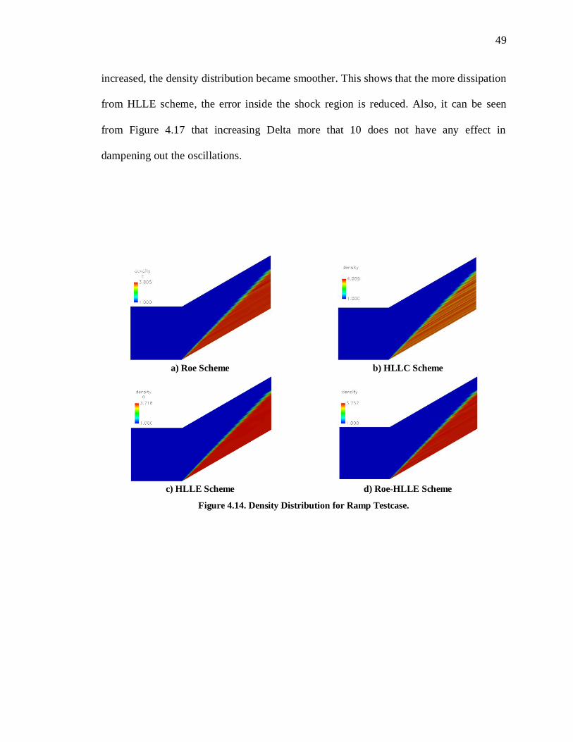
Four different Riemann solvers and four different Delta values for the HLLC+
scheme were used to solve the inviscid ramp testcase. Figure 4.14 and Figure 4.15 show
the density contours from the simulations using these different numerical schemes. The
density distributions along the line of interent, shown by a red line in Figure 4.13, are
depicted inError! Reference source not found. Figure 4.16 and Figure 4.17. These
figures has been focused at the inside of the region between the shock and the wedge to
clearly see the variation of density. It can be seen from Figure 4.16 Error! Reference
ource not found. that the predicted density distributions for HLLC and Roe scheme give
the most disturbances behind the shock region. Also, it can be seen that HLLE and
adaptive Roe-HLLE give a smoother density oscilattion in that region. The results from
the HLLC+ scheme different Delta values are shown in Figure 4.17. The lowest value of
Delta gives the most density disturbances because of less contribution of HLLE flux for
lower value of Delta. The HLLE flux is more dissipative than HLLC scheme and
therefore less dampening effects for lower value of Delta. As the value of Delta
Page 59
49
increased, the density distribution became smoother. This shows that the more dissipation
from HLLE scheme, the error inside the shock region is reduced. Also, it can be seen
from Figure 4.17 that increasing Delta more that 10 does not have any effect in
dampening out the oscillations.
a) Roe Scheme b) HLLC Scheme
c) HLLE Scheme d) Roe-HLLE Scheme
Figure 4.14. Density Distribution for Ramp Testcase.
Page 60
50
a) Delta = 1 b) Delta = 5
c) Delta = 10 d) Delta = 20
Figure 4.15. Density Contour for Combination HLLC+ with Different Delta Values.
Figure 4.16. The Density Values Inside the Shock Region.
Page 61
51
Figure 4.17. Density Plot for Different Delta Values for HLLC+ Scheme.
Figure 4.18. Density Plot Comparison for HLLE, Roe-HLLE, and HLLC+ Scheme.
Page 62
52
Figure 4.18 shows a comparison between HLLE, adaptive Roe-HLLE, and
HLLC+ with a Delta of 20. HLLE scheme gives the smoothest density distribution and
also confirms that adding dissipation could remove a spurious solution inside a strong
shock.
4. 4. Effect of Numerical Flux Evaluation on Solution Accuracy
A laminar hypersonic flow past a cylinder is used as a benchmark testcase to
investigate carbuncle phenomenon for different Riemann solvers. The details of the
experimental data is available in Holden et al.[31]
. The freestream flow Mach number,
temperature, Reynolds number per meter, and specific heat for this testcase are 16.01,
43.2 K, 91,100, and 1.4 respectively. The effect of numerical schemes on the solution
accuracy is discussed below. A three dimensional single block mesh with 40,542 nodes
and 25,704 cells was used for the simulation. The single block mesh was used for the
study to avoid any uncertainties associated with overset meshes. The simulations were
carried out using second order spatial discretization and the results of the predicted
pressure contours for the seven different numerical schemes are presented in Figure 4.19.
Page 63
53
Roe HLLC HLL HLLE Van Leer
Roe-HLLE HLLC+
Figure 4.19. Comparison of Pressure Contour from Simulations using Different Flux Evaluations.
It can be seen from the figure that the Roe and HLLC scheme produces spurious
predictions, while HLL, HLLE, and van Leer giving a more reasonable contour. Both the
adaptive Roe-HLLE and HLLC+ predict a smooth variation of the pressure without
Page 64
54
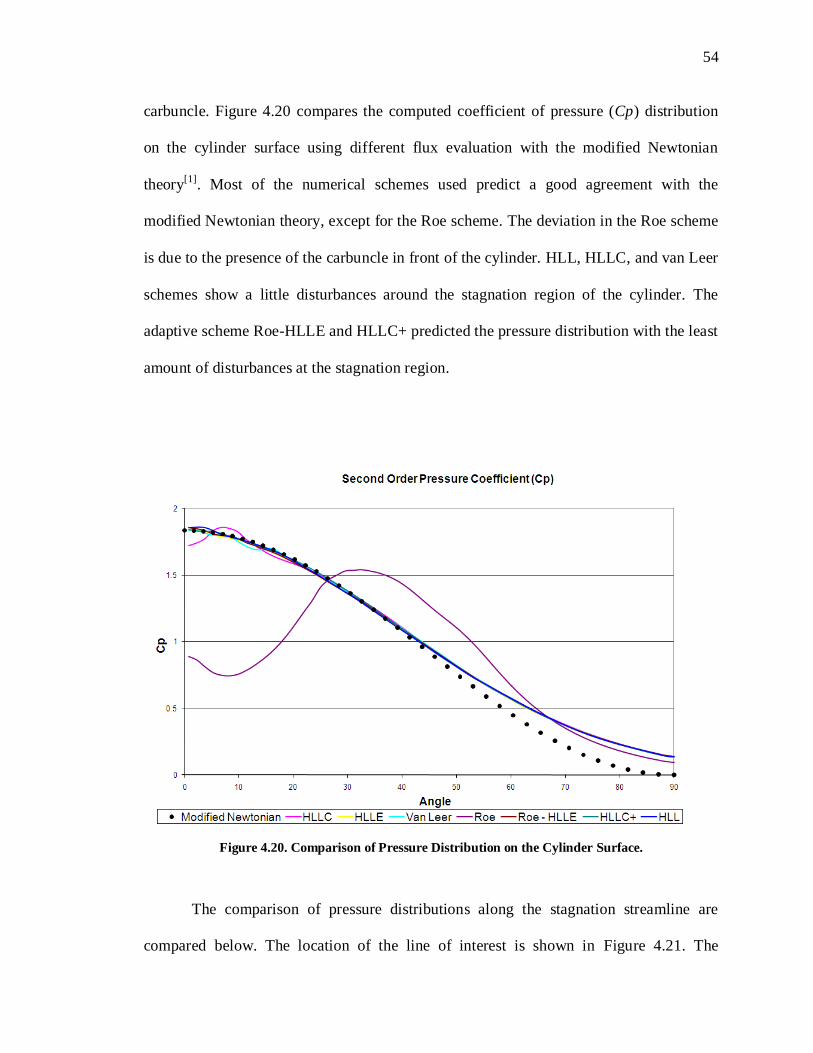
carbuncle. Figure 4.20 compares the computed coefficient of pressure (Cp) distribution
on the cylinder surface using different flux evaluation with the modified Newtonian
theory[1]
. Most of the numerical schemes used predict a good agreement with the
modified Newtonian theory, except for the Roe scheme. The deviation in the Roe scheme
is due to the presence of the carbuncle in front of the cylinder. HLL, HLLC, and van Leer
schemes show a little disturbances around the stagnation region of the cylinder. The
adaptive scheme Roe-HLLE and HLLC+ predicted the pressure distribution with the least
amount of disturbances at the stagnation region.
Figure 4.20. Comparison of Pressure Distribution on the Cylinder Surface.
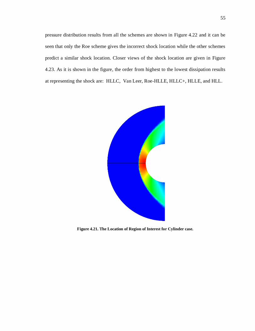
The comparison of pressure distributions along the stagnation streamline are
compared below. The location of the line of interest is shown in Figure 4.21. The
Page 65
55
pressure distribution results from all the schemes are shown in Figure 4.22 and it can be
seen that only the Roe scheme gives the incorrect shock location while the other schemes
predict a similar shock location. Closer views of the shock location are given in Figure
4.23. As it is shown in the figure, the order from highest to the lowest dissipation results
at representing the shock are: HLLC, Van Leer, Roe-HLLE, HLLC+, HLLE, and HLL.
Figure 4.21. The Location of Region of Interest for Cylinder case.
Page 66
56
Figure 4.22. Pressure Distribution accros the Line of Interest at 0 degree
Figure 4.23. Closer Look of Pressure Distribution accros the Line of Interest at 0 degree.
Page 67
57
The heat transfer predictions for these fluxes were also studied. The setting of the
boundary condition at the cylinder surface is taken as an isothermal surface with the
freestream temperature. Thus, the prediction of heat flux was miscalculated because of
the wrong wall temperature used for the simulation as compared to the experimental
setup. Because of the implementation of the correct temperature at the cylinder surface
needed to be revisited, the preliminary results are given in the future work section in
Chapter 5.
4. 5. Overset Mesh Interpolation Study using Conserved and Primitive Variables.
Before applying the overset mesh method to solve hypersonic problems, the
interpolation method for the overset mesh framework needs to be validated. A simple
case of a shock moving across a region of overset mesh is used for studying the overset
interpolation method. The mesh used for the study is shown in Figure 4.24. The
conserved variable interpolation resulted in spurious values at the interface region
resulting in a non-physical solution as shown in Figure 4.24b. The result from primitive
variable interpolation for the transfer of information across overlapping region is shown
in Figure 4.24c. It can be observed that when interpolating with the primitive variables,
the shock moves through the overset region without any non-physical disturbances.
Another testcase was studied for the evaluation of interpolation accuracy is a flow
over a 45o wedge
[37]. The mesh used for this simulation is shown in Figure 4.25. The
overset mesh interpolation method using conserved variables gave spurious unphysical
values at the fringes points as shown in Figure 4.25b. With primitive variable
Page 68
58
interpolation, the values at the fringes points become smooth and realistic as shown in
Figure 4.25c. Therefore the overset simulations presented in the following sections are
carried out using primitive variable interpolation.
a) Overset Mesh b) Density Contours with
Conserved Variables Interpolation
c) Density Contours with
Primitive Variables
Interpolation
Figure 4.24. Simulation of Moving Shock on Overset Mesh Assembly.
a) Overset Grid System b) Density Contours with
Conserved Variables
Interpolation
c) Density Contours with
Primitive Variables
Interpolation
Figure 4.25. Simulations of Shock Wedge Interaction using Overset Meshes.
4. 6. Overset Mesh Study on a Hypersonic Cylinder
From the results of single mesh, the adaptive scheme Roe-HLLE and HLLC+
give promising result in preventing the carbuncle and provide realistic pressure
predictions. The Roe-HLLE scheme was used for study the effect of interpolation
Page 69
59
schemes, mesh topology, and mesh resolution on solution accuracy. The hypersonic
cylinder test case described in Section 4.4 is used for this study also. A detailed view of
one of the meshes used for this study together with the fringe points and blanked points is
shown in Figure 4.26. In the figure the mesh points tagged as black squares represent the
fringe points for the cylinder mesh where the variables are interpolated from the
background mesh. The mesh points tagged as red squares represent the fringe points
where for the background mesh the variables are interpolated from the cylinder mesh.
Mesh points tagged as green squares represent blanked cells in the background mesh,
where the computations are not carried out.
a) Overset Assembly b) Close View of Overset Assembly
Figure 4.26. Overset Grid Assembly for Structured Background and Body Fitted Meshes.
4. 6. 1. Effect of Different Overset Mesh Interpolations on Solution Accuracy
An accurate interpolation of information between meshes in the overlapping
region is the most crucial process in the overset mesh method. The influence of different
overset mesh interpolation method on the accuracy of pressure is analyzed using a
Page 70
60
structured background mesh and hybrid body fitted mesh. The mesh contains 101,441
cells for the background mesh and 10,692 cells for the body fitted mesh. The overall
view of the overset mesh and details of the overset assembly are shown in Figure 4.27a
and b respectively. The interpolation approaches used in this study include simple
inverse distance weighting, weighted least-square approach, Laplacian weighting, and
clipped Laplacian weighting. The inverse distance interpolation scheme employs the
weighting factor based on the inverse of the distance between the points where the data is
to be interpolated and the data points within the search radius are used for interpolation.
The weights for the inverse distance weighting procedure are bounded between (0, 1) and
hence are monotone (the interpolated value is between the minimum and maximum
values of the donor member values). For the least square based interpolation, the data at
each grid point is expressed in terms of the gradient and a value at the reference point.
The reference point can be any arbitrary data point in the set used for interpolation. The
resulting over-determined system is solved for the gradient using the least square
approach and the Graham Schmidt method. The least square approach for data
interpolation can have weights that are greater than one and may not be monotone, which
can lead to stability problems in the flow solver. To alleviate this problem, the
interpolated value is limited between the extrema of the donor member values. The
Laplacian interpolation scheme is based on the weighted averaging procedure, which
estimates the value at an interpolated cell by a weighted average of the surrounding cells.
The weight factors are derived such that the Laplacians are satisfied. Clipped Laplacian
approach is a variation of the Laplacian scheme in which all the weights are clipped in
the range (0, 2). A typical pressure distribution in front of the cylinder is shown in Figure
Page 71
61
4.27c. It can be seen from the figure that the shockwave propagates through the
overlapping region without any disturbances. The predicted pressure distribution on the
cylinder surface using different interpolation schemes are compared in Figure 4.28. The
predicted pressure distribution contours for all different interpolation methods behave
very similar with little disturbances around the stagnation region of the cylinder.
a) Overall Mesh b) Overlapping Region (c) Pressure Contour
Figure 4.27. Overset Mesh with Structured Background Mesh and Hybrid Body Fitted Mesh and
Pressure Distribution from the Simulation.
Page 72
62
Figure 4.28. Coefficient of Pressure across the Cylinder Surface for Different Interpolation Scheme.
4. 6. 2. Effect of Different Overset Mesh Topologies on Solution Accuracy
A mesh topology study is performed to observe the effect of different mesh
topology to the solution accuracy. The study the effect of mesh topology used two
different overset meshes has been created. Theses meshes are 1) structured background
mesh and structured cylinder mesh and 2) structured background mesh and hybrid
cylinder mesh. Details of these overset meshes are given in Table 4.2. The pressure
distribution on the cylinder surface using the overset simulations are being compared
with the result from the single mesh solution and the experimental data in Figure 4.29.
The results are in good agreed with the modified Newtonian theory and single mesh
result. The results show that by changing the mesh topology do not affect the prediction
of pressure distribution.
Cp Distribution for Overset Grid
0
0.2
0.4
0.6
0.8
1
1.2
1.4
1.6
1.8
2
0 10 20 30 40 50 60 70 80 90
Angle
Cp
Modified Newtonian Inverse Distance Clipped Laplacian Laplacian Least Square
Page 73
63
Table 4.2. Mesh Information for Overset Meshes with Different Topology.
Overset Grids Number of Nodes Number of Cells
Structure – Structure 172,026 111,200
Prism – Structure 232,004 292,770
Figure 4.29. Pressure Distribution using Overset Meshes with Different Mesh Topologies.
4. 6. 3. Effect of Different Overset Non-Dimensional Wall Distance on Solution Accuracy
The effect of non-dimensional wall distance (y+) on the solution accuracy was
studied using different normal distances of the first point off the cylinder on an overset
mesh with a structured background and cylinder meshes. Four different y+ value were
used in the simulations were 2.3, 1.8, 1.7, and 0.8. The diameter of the cylinder was taken
as one unit. A geometric progression with a progression ratio of 1.1 was used for
distributing points in the radial direction. The details of the meshes used for the
simulations are given in Table 4.3. The computed pressure distribution on the cylinder
from these simulations is compared with the data from the modified Newtonian theory in
Figure 4.30. The computed pressure distribution from all the four overset meshes are in
Cp Distribution for Overset Grid
0
0.2
0.4
0.6
0.8
1
1.2
1.4
1.6
1.8
2
0 10 20 30 40 50 60 70 80 90
Angle
Cp
Modified Newtonian Single Grid Structure - Structure Prisms - Structure
Page 74
64
good agreement with the modified Newtonian theory. It can be concluded that the mesh
resolution has very little effect on predicting the pressure distribution.
Table 4.3. Structure-Structure Overset Mesh with Different y+ to the Wall Information.
y+
Normal
Distance
to the Wall
Background Mesh Body Fitted Mesh (Cylinder)
Topology
Number
of Cells
Number
of Nodes Topology
Number
of Cells
Number
of Nodes
2.3 0.002 Structure 101,442 153,600 Structure 6,664 10,440
1.7 0.001 Structure 101,442 153,600 Structure 8,330 12,960
1.4 0.0005 Structure 101,442 153,600 Structure 9,996 15,480
0.8 0.00025 Structure 101,442 153,600 Structure 11,662 18,000
Figure 4.30. Comparison of Pressure Distribution from Overset Meshes with Different Mesh.
4. 7. Shock/Shock Interaction in a Laminar Hypersonic Flow
A shock/shock interaction heat transfer study is very critical in developing
hypersonic vehicles because of the high temperature produced in the interaction region.
According to Edney[32]
in a shock/shock interaction study, there are six different
classifications of shock/shock interaction patterns which depends on the position of the
Cp Distribution for Overset Grid with Differen Normal Distance to the Wall
0
0.2
0.4
0.6
0.8
1
1.2
1.4
1.6
1.8
2
0 10 20 30 40 50 60 70 80 90
Angle
Cp
Modified Newtonian 0.002 0.001 0.0005 0.00025
Page 75
65
incoming shock pattern. Type III and type IV interactions are the most critical, since they
are characterized by the largest values of wall pressure and heat transfer. In order to
study this type of shock/shock interaction, several experiments have been conducted at
ONERA in wind tunnel R5Ch[33]
. The experimental set up of the shock/shock interaction
is shown in Figure 4.31, and all the dimensions are in millimeters. The shock is generated
using an isosceles triangle prism with a base of 100 mm and a leading edge angle of 10 o
.
In this experiment, the shock generator was rotated by 10o
as shown in Figure 4.31. The
angle of the shock created is 25o. The freestream temperature of 52.5K, pressure of 5.9
Pa, Mach number of 9.95, and Reynolds number per meter of 1.66 x 10⁵ is used for the
experiment.
Figure 4.31. Shock/Shock Interactions Experimental Set Up at ONERA.
(Picture is reproduced from D’Ambrosio[33]
)
An overset mesh approach is used for performing the shock/shock interaction
study. The overset meshes used for the study are shown in Figure 4.32 and Figure 4.33.
In Figure 4.32, the shock generator was rotated by an angle 10 degrees, while in Figure
4.33 the shock generator was rotated by 12 degrees. The pressure contours from the
simulations using these meshes are also plotted in Figure 4.32 and Figure 4.33. It can be
noted that the shock created by the shock generator passes smoothly across the
Page 76
66
overlapping region to the cylinder. However, the orientation of the shock generator with
10 degrees produces an Edney Shock Type II shock/shock interaction pattern, while the
12 degree orientation produces Edney Shock Type IV.
Figure 4.32. Pressure Contour for Shock/Shock Interaction Study with 20o Shock Generator.
Page 77
67
Figure 4.33. Pressure Contour for Shock/Shock Interaction Study with 22o Shock Generator.
The computed pressure contours are compared with the results from
D‟Ambrosio[33]
in Figure 4.34. The minimum, maximum, and average y+ values for the
shock/shock interaction simulation case were 0.033, 0.7, and 0.184 respectively. The
Type IV shock/shock interaction pattern compares well with D‟Ambrosio‟s results as
shown in Figure 4.34. The pressure distribution and heat transfer results are shown in
Figure 4.35 and Figure 4.36 respectively, where the highest peaks for both predictions are
shifted downward as compared with the experimental result. The error could be caused
by changing the angle of the shock from the shock generator or slight variation in
incident shock strength.
Page 78
68
a) Type IV Shock/Shock Interactions by
D’Ambrosio (Picture is reproduced from
D’Ambrosio*)
b) Type IV Shock/Shock Interactions.
Figure 4.34. Close View at the Shock/Shock Interaction Patterns.
Figure 4.35. Pressure Distribution on a Cylinder Surface.
Page 79
69
Figure 4.36. Heat Transfer Distribution on a Cylinder Surface.
Page 80
70
5. CONCLUSION AND FUTURE WORK
Most commonly used shock capturing schemes for transonic and supersonic
problems suffer from spurious solution when used for hypersonic problems. The
phenomenon is known as carbuncle phenomenon. In order to prevent the carbuncle
phenomenon, there are many aspects that need to be carefully chosen. High dissipative
Riemann solver, such as the HLLE scheme, is proven to be free from the carbuncle
effect. However, the quality of the solution for such dissipative scheme is questionable
because of the lack of accuracy inside the boundary layer calculation. There are two
major fixes that have been proposed in the last decade: 1) the entropy fix approach and 2)
adaptive scheme approach. The entropy fix approach tries to add numerical dissipation to
the convective part of the governing equations. This approach can be very difficult to
implement and also violates the real physical behavior of the governing equations. The
second approach is simpler than the first one. The adaptive approach uses a more
dissipative Riemann Solver in the strong shock region and uses a more accurate one in
rest of the domain. Two adaptive schemes, Roe-HLLE and HLLC+, are implemented and
evaluated for numerical accuracies.
The results from validation study show that both adaptive scheme prevent the
carbuncle phenomenon and give better pressure predictions. It is also shown that adaptive
Roe-HLLE and HLLC+ schemes do not require mesh alignment to produce good quality
Page 81
71
solution. The benefit of using the combination of HLLC+ than Roe-HLLE is that both the
HLLC and HLLE schemes are positively conserved which lead to a better stability. A
minor drawback of using both adaptive schemes is the difficulty on deciding the
switching parameter values. Currently value used for the switching parameter is chosen
based on experience and it will require different value for each specific case.
The use of overset meshes could benefit the mesh generation process, especially
for complex geometry and moving body problems. The most important parameter that
needs to be carefully checked when using overset mesh framework is the interpolation
method between the overset meshes. A primitive variable interpolation has shown better
accuracy for testcases involving shock across overlapping region as compared to
conserved variable interpolation. The mesh size in the overlapping region needs to be
checked carefully to get the best interpolation solution. In order to get the best shock
representation across the overlapping region, mesh size need to be similar for each mesh
in the overset system. A study has been conducted to investigate the effect of
interpolation schemes, mesh topology, and mesh resolution on solution accuracy. None
of these variables has shown any significant effect on the prediction of pressure
distribution for the testcases that were used in this study.
Predicting the heat transfer in a hypersonic flow is a challenging task and is
tougher than other flow variables. From the heat transfer study, it was noted that different
mesh topology and overset mesh interpolation method did not affect the heat transfer
predictions. However, the heat transfer predictions were improved by decreasing the
distance of the first point off the wall.
Page 82
72
5. 1. Future Work
Heat transfer prediction for hypersonic flow over a cylinder has been studied
using single and overset meshes. The boundary condition for the cylinder surface is taken
as an isothermal surface with wall temperature as the freestream temperature. However,
the experimental investigation[31]
was carried out using a different temperature for the
cylinder. Therefore, the predicted values of the heat flux were inaccurate because of the
incorrect wall temperature used for the simulation as compared to the experiment.
Numerical experiments has been conducted to compare the predicted heat flux
distribution from a single block mesh with overset mesh simulations using different
interpolation schemes, mesh topology, and mesh resolution. In all these calculations, the
wall temperature is taken as the freestream temperature. In the first step of this study,
results from different numerical schemes were compared using a single mesh and the
comparison of the predicted heat transfer is shown in Figure 5.1. The adaptive scheme
Roe-HLLE and HLLC+ give the smoothest distribution of the heat flux over the cylinder.
In the second step of the study, Roe-HLLE scheme was used to predict the heat
flux to the cylinder using overset meshes. Three different parameters were used for these
simulations: 1) interpolation schemes, 2) mesh topology, and 3) mesh resolution. The
results from this study are summarized in Figure 5.2 - Figure 5.4. The heat transfer
distributions for all different interpolation method and different mesh topology behave in
a similar fashion with slight disturbances around the stagnation region of the cylinder
(Figure 5.2 and Figure 5.3). The comparison of predicted heat flux using the overset
meshes with different point distribution normal to the wall are shown in Figure 5.4. It
can be seen from the figure that the computed heat flux are getting closer to the
Page 83
73
experimental data as the distance of the first point off the cylinder decreases. It can be
concluded from Figure 5.4 that the non-dimensional wall distance has stronger influence
on solving the heat transfer than pressure distribution.
Figure 5.1. Comparison of Heat Flux Distribution on the Cylinder Surface.
Figure 5.2. Comparison of Heat Flux Predictions from Different Interpolation Techniques.
Heat Transfer Distribution for Overset Grid with Different Interpolation
0
50000
100000
150000
200000
250000
300000
0 10 20 30 40 50 60 70 80 90
Angle
Q (
W/m
^2
)
Holden's Exp Data Inverse Distance Clipped Laplacian Laplacian Least Square
Page 84
74
Figure 5.3. . Comparison of Heat Flux Predictions using Overset Meshes with Different Mesh
Topologies.
Figure 5.4. Comparison of Heat Flux Distribution from Overset Meshes with Different Mesh
Resolution.
Heat Transfer Distribution for Overset Grid with Different Topology Grids
0
50000
100000
150000
200000
250000
300000
0 10 20 30 40 50 60 70 80 90
Angle
Q (
W/m
^2
)
Holden's Exp Data Single Grid Structure - Structure Prisms - Structure
Page 85
75
The boundary condition for isothermal wall has been fixed and numerical
simulations have been carried out for the hypersonic flow past the cylinder using a single
block mesh. New single block mesh with finer non-dimensional wall distance has been
generated to improve the heat transfer predictions. The new mesh consists of 48,000 cells
and 65,556 nodes. Figure 5.5 - Figure 5.7 show the temperature contour, pressure
distribution, and heat transfer distribution on the cylinder surface for different flux
evaluation schemes. Even with the prediction of the pressure distribution agrees with the
modified Newtonian theory, the heat transfer rates are over predicted by all numerical
schemes. The adaptive schemes, Roe-HLLE and HLLC+ schemes, predicts heat transfer
rates within 10-15% accuracy. The heat flux contours for different flux schemes are
shown in Figure 5.8. It can be seen from the figure that the symmetry of the computed
heat flux along the spanwise direction is not preserved by different numerical convective
flux evaluation schemes. In these simulations, three layers of cells have been used along
the spanwise directions. From this figure, it can also be seen that HLLC+ gives a
reasonable and almost symmetric heat transfer contour while others give spurious and
asymmetric contour. The density and pressure contours on the cylinder surface are given
in Figure 5.9 and Figure 5.10. Both results did not show as much disturbances as heat
flux predictions. Therefore, further study is required to evaluate the cause for this
spurious behavior for the heat flux predictions. Also, simulations need to be conducted to
evaluate the effect of different overset parameters on simulation accuracy using corrected
isothermal boundary conditions.
Page 86
76
Figure 5.5. Temperature Contour for Cylinder Testcase with Single Mesh.
Figure 5.6. Cp Value at the Cylinder Surface.
Page 87
77
Figure 5.7. Heat Transfer at the Cylinder Surface.
HLL HLLC HLLE VL Roe Roe-HLLE HLLC+
Figure 5.8. Heat Transfer Contour at Cylinder Surface for Different Flux Schemes.
Page 88
78
HLL HLLC HLLE VL Roe Roe-HLLE HLLC+
Figure 5.9. Density Contour at Cylinder Surface for Different Flux Schemes.
HLL HLLC HLLE VL Roe Roe-HLLE HLLC+
Figure 5.10. Pressure Contour at Cylinder Surface for Different Flux Schemes.
Page 89
79
LIST OF REFERENCES
[1] J.D. Anderson, Hypersonic and High-Temperature Gas Dynamics, American
Institute of Aeronautics and Astronautics, 2006.
[2] Pandolfi, M., and D‟Ambrosio, D., “Numerical Instabilities in Upwind Methods:
Analysis and Cures for the „Carbuncle‟ Phenomenon”, Journal of Computational
Physics, 166, pp. 271-301, 2001.
[3] Trammel, R.W., Nichols, R.H., and Buning, P.G., “Addition of Improved Shock-
Capturing Schemes to OVERFLOW 2.1”, AIAA Papers 2009-3988, 2009.
[4] Koomullil, R.P., “Flow Simulation System for Generalized Static and Dynamic
Grids”, PhD Dissertation, Mississippi State University, May 1997.
[5] Koomullil, R., et al., “Moving-Body Simulations using Overset Framework with
Rigid Body Dynamics”, Mathematics and Computers in Simulation, Vol. 78, 5-6,
pp. 618-626, Sept 2008.
[6] Koomullil, R., et al., “Generalized Overset Grid Framework for Incompressible
Flows”, AIAA 2006-1146, 2006.
[7] Benek, J.A., Steger, J.L., and Dougherty, F.C., “A Flexible Grid Embedding
Technique with Application to the Euler Equations”, AIAA Papers 1983-1944,
1983.
[8] Quattrochi, D.J., “Hypersonic Heat Transfer and Anisotropic Visualization with a
Higher Order Discontinuous Galerkin Finite Element Method”, Master Thesis,
Massachusetts Institute of Technology, June 2006.
[9] Gnoffo, P.A., and White, J.A., “Computational Aerothermodynamics Simulation
Issues on Unstructured Grids”, AIAA Papers 2004-2371, 2004.
[10] Gnoffo, P.A., “Computational Fluid Dynamics Technology for Hypersonic
Applications”, AIAA Papers 2003-3259, 2003.
[11] Gnoffo, P.A., “Simulation of Stagnation Region Heating in Hypersonic Flow on
Tetrahedral Grids”, AIAA 2007-3960, 2007.
[12] Candler, G.V, et al., “Unstructured Grid Approaches for Accurate Aeroheating
Simulations”, AIAA 2007-3959, 2007.
Page 90
80
[13] Peerly, K.M., and Imlay, S.T., “Blunt Body Flow Simulations”, AIAA Papers
1988-2924, 1988.
[14] Quirk, J.J., “A Contribution to the Great Riemann Solver Debate”, International
Journal Numerical Method Fluids 18, 1994.
[15] Liou, M.S, “Mass Flux Schemes and Connection to Shock Instability”, Journal of
Computational Physics, 160, pp. 623-648, 2000.
[16] Ismail, F., “Toward a Reliable Prediction of Shock in Hypersonic Flow:
Resolving Carbuncles with Entropy and Voticity Control”, PhD Dissertation,
2006.
[17] Dumbser, M., Moschetta, J.M., and Gressier, J., “A Matrix Stability Analysis of
the Carbuncle Phenomenon”, Journal of Computational Physics, 197, pp. 647-
670, 2004.
[18] Loh, C.Y., and Jorgenson, P.C.E., “Multi-dimensional Dissipation for Cure of
Pathological Behaviors of Upwind Scheme”, Journal of Computational Physics,
228, pp. 1343-1346, 2009.
[19] Loh, C.Y., and Jorgenson, P.C.E., “A Time-Accurate Upwind Unstructured Finite
Volume Method for Compressible Flow with Cure of Pathological Behaviors”,
NASA/TM-2007-214918, 2007.
[20] Xu, K., “Gas Evolution Dynamics in Godunov-type Schemes and Analysis of
Numerical Shock Instability”, NASA/CR-1999-208985, 1999.
[21] Xu, K., and Li, Z., “Dissipative Mechanism in Godunov-Type Schemes”,
International Journal for Numerical Methods in Fluids, 37, pp. 1-22, 2001.
[22] Henderson, S.J., and Menart, J.A., “Grid Study on Blunt Bodies with the
Carbuncle Phenomenon”, AIAA Papers 2007-3904, 2007.
[23] Kitamura, K., Roe, P., and Ismail, F., “Evaluation of Euler Fluxes for Hypersonic
Flow Computations”, AIAA Journal, Vol. 47., No. 1, Jan 2009.
[24] Xu, K., and Hu, J., “Project Dynamics in Godunov-Type Schemes”, Journal of
Computational Physics, 142, pp. 412-427, 2008.
[25] Noack, R.W., “SUGGAR: A General Capability for Moving Body Overset Grid
Assembly”, AIAA Papers 2005-5117, 2005.
Page 91
81
[26] Noack, R.W., “DiRTlib: A Library to Add an Overset Capability to Your Flow
Solver”, AIAA Papers 2005-5116, 2005.
[27] Milner, J.H., “Computational Aerothermodynamics Datasets for Hypersonic Heat
Transfer on Reentry Vehicles”, AIAA Papers 2005-5911, 2005.
[28] Hyams, D.G., “An Investigation of Parallel Implicit Solution Algorithms for
Incompressible Flows on Unstructured Topologies”, PhD Dissertation,
Mississippi State University, May 2000.
[29] Barth, T.J., and Jespersen, D.C., “The Design and Application of Upwind
Schemes on Unstructured Meshes,” AIAA 89-0366, 1989.
[30] Toro, E.F., “Riemann Solvers and Numerical Methods for Fluid Dynamics: A
Practical Introduction”, 2nd
edition, Springer, Berlin, 1999.
[31] Holden, M.S., Kolly, J.M., and Martin, S.C., “Shock/Shock Interaction Heating in
Laminar and Low-Density Hypersonic Flows”, AIAA Papers 1996-1866, June
1966.
[32] Grasso, F., et al., “Type III and Type IV Shock/Shock Interferences: Theoretical
and Experimental Aspects”, Aerospace Science and Technology, 7, pp. 93-106,
2003.
[33] D‟Ambrosio, D., “Numerical Prediction of Laminar Shock/Shock Interactions in
Hypersonic Flow”, RTO-TR-AVT-007-V3, Jan 2006.
[34] Roe, P.L., “Approximate Riemann Solvers, Parameter Vectors, and Different
Schemes”, Journal of Computational Physics, Vol. 43, pp. 357-372, 1981.
[35] Toro, E.F, Spruce, M., and Speares, W., “Restoration of the Contact Surface in
the HLL-Riemann Solver”, Shock Waves, 4, pp. 25-34, 1994.
[36] Einfeldt, B., “On Godunov-Type Methods for Gas Dynamics”, SIAM Journal on
Numerical Analysis, Vol. 25, No. 2, 1998.
[37] D. L. Zhang and I. I. Glass, “Interferometric investigation of the diffraction of
planar shock waves over a half-diamond cylinder in air”, UTIAS Report No. 322,
March 1988.