energies

Article

Heat-Transfer Characteristics of Liquid Sodium in aSolar Receiver Tube with a Nonuniform Heat Flux

Jing Liu 1, Yongqing He 1,* and Xianliang Lei 2

1 School of Chemical Engineering, Kunming University of Science and Technology, Kunming 650500, China;Jedxy1037@gmail.com

2 State Key Laboratory of Multiphase Flow in Power Engineering, Xi’an Jiaotong University, Xi’an 710049,China; xianlianglei@xjtu.edu.cn

* Correspondence: yqhe@kmust.edu.cn

Received: 7 March 2019; Accepted: 11 April 2019; Published: 14 April 2019�����������������

Abstract: This paper presents a numerical simulation on the heat transfer of liquid sodium in a solarreceiver tube, as the liquid sodium is a promising heat-transfer candidate for the next generationsolar-power-tower (SPT) system. A comparison between three mediums—solar salt, Hitec and liquidsodium—is presented under uniform and nonuniform heat-flux configurations. We studied theeffects of mass flow rate (Qm), inlet temperature (Tin), and maximum heat flux (qomax), on the averageheat-transfer coefficient (h) and the friction coefficient (f ) of the three mediums. The results show thatthe h of liquid sodium is about 2.5 to 5 times than other two molten salts when Tin is varying from 550to 800 K, Qm is 1.0 kg/s, and qomax is 0.1 MW/m2. For maximum heat fluxes from 0.1 to 0.3 MW/m2,the h of liquid sodium is always an order of magnitude larger than that of Hitec and Solar-Salt (S-S),while maintaining a small friction coefficient.

Keywords: solar-power tower; liquid sodium; solar salt; Hitec; heat flux

1. Introduction

Compared to the parabolic trough, Fresnel and dish collectors, the solar-power-tower (SPT) planthas the remarkable advantages, such as lower electricity cost, large-scale power generation and higherefficient thermodynamic cycles [1–3]. The SPT is equipped with a large number of heliostats on theground, each with a tracking mechanism that accurately reflects the reflection of sunlight onto thereceiver at the top of a tall tower. The concentrating magnification on the receiver can exceed 1000times. One typical arrangement of the SPT receivers is the external tubular receiver designed for SolarTwo project, in which only half of the surface of the tube is exposed to solar irradiation. This may bringabout many problems, such as aggravating the plastic deformation of the receiver tube, facilitatingdegradation of the selective absorptive coating and decreasing the allowable solar heat flux [4,5]. Sincethe nonuniform solar heat flux tends to cause the temperature inhomogeneity of the heat-transfer fluid(HTF) and, further, the thermal stress on the heat-transfer tubes, a much broader range of operationaltemperatures is required. The liquid metal as the promising candidate for the exposed cylindrical heatabsorber of SPT has been proposed [6].

Nitrate salts have been used as HTFs and thermal storage mediums for decades in the concentratingSPT industry. The most commonly used HTFs are solar salt (S-S, 60% NaNO3 and 40% KNO3) andHitec (53% KNO3 + 40% NaNO2 + 7% NaNO3). Both the nitrate salt mixtures will decompose above873 ◦K, which has seriously limited the overall efficiency in the SPT system. Furthermore, recentresearch efforts have shown that the nitrate salts are more suitable for use in parabolic trough systemsdue to their low working temperature [7]. However, the next-generation SPT systems require a higherincident peak flux and operating temperature. If the liquid metal is the heat-transfer fluid, it can

Energies 2019, 12, 1432; doi:10.3390/en12081432 www.mdpi.com/journal/energies

Energies 2019, 12, 1432 2 of 16

provide an incident peak flux above 0.6 MW/m2. Liquid sodium (Na), characterized by chemicalstability at temperatures up to near 1173 ◦K has a lower melting point to 371 ◦K [8], as well as superiorthermal conductivity and low Prandtl number. The material properties mentioned above can largelyimprove heat transfer when compared to conventional fluids such as oil or salt mixtures [9]. In fact,during the early years of the development of central receiver systems (CRSs), liquid sodium wasone of the prominent HTFs under investigation. Indeed, several test projects have been developed,and the efficiency was obtained at 88%–96% in the 1980s [10]. However, the disadvantage of liquidsodium is its high combustibility when in contact with water even if no air. Fortunately, special andprotective measures have also been developed from previous experiences [11]. Also, this technologyhas continued to be investigated by several institutions around the world [12–14]. Besides, furtherwork has reported that liquid metals have attractive properties for CSP applications [15,16]. Recently,Amy et al. [17] demonstrated how a ceramic, mechanical pump that can be used to continuouslycirculate liquid metal at temperatures of around 1473 ◦K–1746 ◦K. This study solves the problem thatcollecting, transporting, storing liquid metal above 1300 ◦K brings.

The prediction of heat transfer of liquid metal has been the subject of many investigations.DeAngelis et al. [18] have examined using a liquid metal as heat-transfer fluid in conjunction with areceiver. It is feasible to reach temperatures of 1623 ◦K at greater than 90% efficiency. Boerema et al. [15]compared liquid sodium and Hitec, and the use of liquid sodium can achieve 57% absorber areareduction and 1.1% efficiency improvement. Even if liquid sodium is an excellent heat-transfer medium,the specific application background was not mentioned in the paper. Pacio et al. [19,20] summarizedthe current state-of-the-art of liquid metals (LMs) as HTFs in solar power plants.

Additionally, the liquid sodium (Na) was proposed as an efficient HTF to allow extending thedesign ranges, and able to contribute to the development of next-generation SPT. Matsubara et al. [21]studied the spanwise heat transport in turbulent channel flow with Prandtl numbers ranging from 0.025to 5.0. It is regrettable that they do not compare the heat-transfer property with traditional heat-transferfluid (e.g., solar salts). Rodríguez-Sanchez et al. [22,23] focused on the thermal, mechanical andhydrodynamic analysis associated to the nonuniformity of the heat flux, and they also considered thethermal field and thermal stresses along the solid wall [24].

A higher cost, more complex system and security issues are factors that have to be considered forthe experimental research on liquid metal.

Therefore, numerical simulation is an effective research method [25,26]. In this work, we presenta numerical simulation on the heat transfer of liquid sodium under nonuniform heat flux. A physicalmodel of a single tube is established to investigate the heat-transfer performance of the receiver tube,and two other commonly used heat-transfer media, Hitec and solar salt, are also to be considered. First,we built solar heat-flux distributions on the whole absorber outer wall and circumferential variation ofheat flux on the inner wall of the tube. Then, the heterogeneity of the temperature on the circumferentialtangent plane and the solid wall is presented. Cloud images show the wall temperature distribution ofthe three HTFs. The temperature difference (Θ-Θref) of the three HTFs along the circumferential angleis compared when qomax is 0.1 MW/m2, Re is ranging from 10,000 to 30,000, and inlet temperatureis 550 ◦K. Last, the influence of three parameters, Qm (1.0 to 3.0 kg/s), qomax (0.1 to 0.3 MW/m2), Tin(550 ◦K to 800 ◦K) on the heat-transfer characteristics of sodium, S-S and Hitec are discussed. Thisresearch can offer technical references for the design and construction of experimental facilities.

2. Mathematical model

2.1. Physical Model

The research background of this study is the heat receiver of the solar-power-tower system(Figure 1a). Since the collector is cylindrical and the fluid flows serpentinely in the collector tube, weinvestigate only the single collector tube (Figure 1b).

Energies 2019, 12, 1432 3 of 16Energies 2019, 12, x FOR PEER REVIEW 3 of 16

(a) (b)

Figure 1. (a) Solar power tower system; (b) Exposed cylindrical heat receiver and a single receiver tube

We consider the conjugate heat-transfer problem of a receiver tube subject to inhomogeneous heat flux along the axial direction (z), circumferential direction (θ), and radial direction (r). The heat transport from the regional source (see Figure 2) contains three orthogonal components. The outer diameter (R) of the geometric model is 20 mm, and the tube length is 100R. The effect of different thermal boundary conditions on the heat-transfer performance of the collector tube is discussed.

Figure 2. Schematic diagram of tower solar collector.

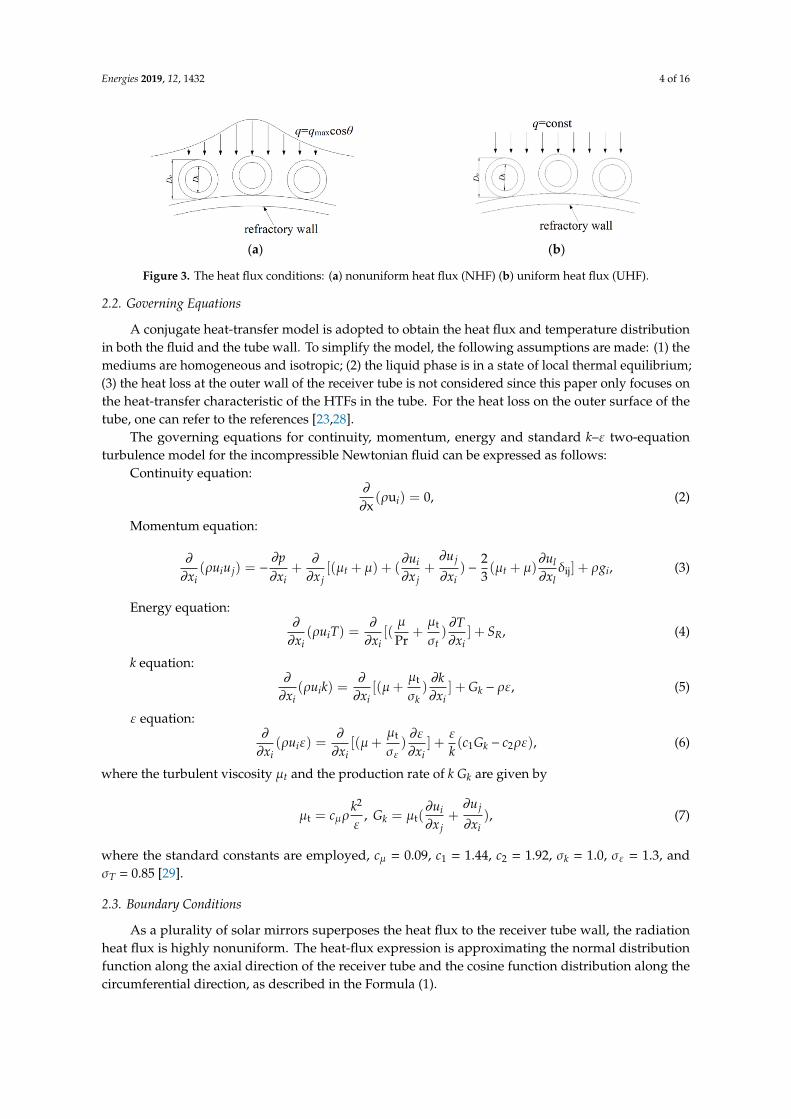
As shown in Figure 3, this paper deals with two heat-flux conditions of the turbulent-flow model:

(a) A cosine heat flux (see Equation (1)) [27] is imposed on one half of the wall of the tube, while the other half is considered adiabatic.

( )θ θ

θ

− ⋅ − ⋅ ⋅ ≥= <

29 12

max e cos , cos 00, cos 0

z

oqq (1)

where the qomax is the maximum heat flux on the wall of the collector tube, θ is the circumferential angle, and z is the length along the axial direction of the receiver tube.

Figure 1. (a) Solar power tower system; (b) Exposed cylindrical heat receiver and a single receiver tube

We consider the conjugate heat-transfer problem of a receiver tube subject to inhomogeneousheat flux along the axial direction (z), circumferential direction (θ), and radial direction (r). The heattransport from the regional source (see Figure 2) contains three orthogonal components. The outerdiameter (R) of the geometric model is 20 mm, and the tube length is 100R. The effect of differentthermal boundary conditions on the heat-transfer performance of the collector tube is discussed.

Energies 2019, 12, x FOR PEER REVIEW 3 of 16

(a) (b)

Figure 1. (a) Solar power tower system; (b) Exposed cylindrical heat receiver and a single receiver tube

We consider the conjugate heat-transfer problem of a receiver tube subject to inhomogeneous heat flux along the axial direction (z), circumferential direction (θ), and radial direction (r). The heat transport from the regional source (see Figure 2) contains three orthogonal components. The outer diameter (R) of the geometric model is 20 mm, and the tube length is 100R. The effect of different thermal boundary conditions on the heat-transfer performance of the collector tube is discussed.

Figure 2. Schematic diagram of tower solar collector.

As shown in Figure 3, this paper deals with two heat-flux conditions of the turbulent-flow model:

(a) A cosine heat flux (see Equation (1)) [27] is imposed on one half of the wall of the tube, while the other half is considered adiabatic.

( )θ θ

θ

− ⋅ − ⋅ ⋅ ≥= <

29 12

max e cos , cos 00, cos 0

z

oqq (1)

where the qomax is the maximum heat flux on the wall of the collector tube, θ is the circumferential angle, and z is the length along the axial direction of the receiver tube.

Figure 2. Schematic diagram of tower solar collector.

As shown in Figure 3, this paper deals with two heat-flux conditions of the turbulent-flow model:(a) A cosine heat flux (see Equation (1)) [27] is imposed on one half of the wall of the tube, while

the other half is considered adiabatic.

q =

qomax · e−92 ·(z−1)2

· cosθ, cosθ ≥ 00, cosθ < 0

(1)

where the qomax is the maximum heat flux on the wall of the collector tube, θ is the circumferentialangle, and z is the length along the axial direction of the receiver tube.

(b) The heat flux to the bright side is constant, and the backlight side is an adiabatic.

Energies 2019, 12, 1432 4 of 16Energies 2019, 12, x FOR PEER REVIEW 4 of 16

(b) The heat flux to the bright side is constant, and the backlight side is an adiabatic.

(a) (b)

Figure 3. The heat flux conditions: (a) nonuniform heat flux (NHF) (b) uniform heat flux (UHF).

2.2. Governing Equations

A conjugate heat-transfer model is adopted to obtain the heat flux and temperature distribution in both the fluid and the tube wall. To simplify the model, the following assumptions are made: (1) the mediums are homogeneous and isotropic; (2) the liquid phase is in a state of local thermal equilibrium; (3) the heat loss at the outer wall of the receiver tube is not considered since this paper only focuses on the heat-transfer characteristic of the HTFs in the tube. For the heat loss on the outer surface of the tube, one can refer to the references [23,28].

The governing equations for continuity, momentum, energy and standard k–ε two-equation turbulence model for the incompressible Newtonian fluid can be expressed as follows:

Continuity equation:

ρ∂ =∂ i( u ) 0

x, (2)

Momentum equation:

ρ μ μ μ μ δ ρ∂∂ ∂∂∂ ∂= − + + + + − + +

∂ ∂ ∂ ∂ ∂ ∂ ij2( ) [( ) ( ) ( ) ]3

ji li j t t i

i i j j i l

uu upu u g

x x x x x x, (3)

Energy equation: μμρσ

∂ ∂ ∂= + +∂ ∂ ∂

t( ) [( ) ]Pri R

i i t i

Tu T Sx x x

, (4)

k equation: μ

ρ μ ρεσ

∂ ∂ ∂= + + −∂ ∂ ∂

t( ) [( ) ]i ki i k i

ku k Gx x x

, (5)

ε equation:

ε

μ ε ερ ε μ ρεσ

∂ ∂ ∂= + + −∂ ∂ ∂

t1 2( ) [( ) ] ( )i k

i i i

u c G cx x x k

, (6)

where the turbulent viscosity μt and the production rate of k Gk are given by

μμ ρε

=2

tkc , μ

∂∂+

∂ ∂t= ( )jik

j i

uuG

x x, (7)

where the standard constants are employed, cμ =0.09, c1 =1.44, c2 =1.92, σk =1.0, σɛ =1.3, and σT =0.85 [29].

2.3. Boundary Conditions

As a plurality of solar mirrors superposes the heat flux to the receiver tube wall, the radiation heat flux is highly nonuniform. The heat-flux expression is approximating the normal distribution function along the axial direction of the receiver tube and the cosine function distribution along the circumferential direction, as described in the formula (1).

It is also convenient to define the total heat flux applied to the outer surface, and note that the energy conservation in the solid implies that:

Figure 3. The heat flux conditions: (a) nonuniform heat flux (NHF) (b) uniform heat flux (UHF).

2.2. Governing Equations

A conjugate heat-transfer model is adopted to obtain the heat flux and temperature distributionin both the fluid and the tube wall. To simplify the model, the following assumptions are made: (1) themediums are homogeneous and isotropic; (2) the liquid phase is in a state of local thermal equilibrium;(3) the heat loss at the outer wall of the receiver tube is not considered since this paper only focuses onthe heat-transfer characteristic of the HTFs in the tube. For the heat loss on the outer surface of thetube, one can refer to the references [23,28].

The governing equations for continuity, momentum, energy and standard k–ε two-equationturbulence model for the incompressible Newtonian fluid can be expressed as follows:

Continuity equation:∂∂x

(ρui) = 0, (2)

Momentum equation:

∂∂xi

(ρuiu j) = −∂p∂xi

+∂∂x j

[(µt + µ) + (∂ui∂x j

+∂u j

∂xi) −

23(µt + µ)

∂ul∂xl

δij] + ρgi, (3)

Energy equation:∂∂xi

(ρuiT) =∂∂xi

[(µ

Pr+µt

σt)∂T∂xi

] + SR, (4)

k equation:∂∂xi

(ρuik) =∂∂xi

[(µ+µt

σk)∂k∂xi

] + Gk − ρε, (5)

ε equation:∂∂xi

(ρuiε) =∂∂xi

[(µ+µt

σε)∂ε∂xi

] +εk(c1Gk − c2ρε), (6)

where the turbulent viscosity µt and the production rate of k Gk are given by

µt = cµρk2

ε, Gk = µt(

∂ui∂x j

+∂u j

∂xi), (7)

where the standard constants are employed, cµ = 0.09, c1 = 1.44, c2 = 1.92, σk = 1.0, σε = 1.3, andσT = 0.85 [29].

2.3. Boundary Conditions

As a plurality of solar mirrors superposes the heat flux to the receiver tube wall, the radiationheat flux is highly nonuniform. The heat-flux expression is approximating the normal distributionfunction along the axial direction of the receiver tube and the cosine function distribution along thecircumferential direction, as described in the Formula (1).

Energies 2019, 12, 1432 5 of 16

It is also convenient to define the total heat flux applied to the outer surface, and note that theenergy conservation in the solid implies that:

Q =

∫ π

0q0(θ)R0dθ = 2qomaxR0, (8)

where the total heat flux (Q) is kept constant for all the cases presented here, and R0 = 20 mm.Considering the wall temperature of the tube varies with the time and heat flux, to improve the

accuracy and practicability of the numerical calculation, we adopted the formulas shown in Table 1 toevaluate the thermophysical properties of HTFs. The collector tube material is 316 L stainless steel,and its thermal conductivity (ks) is 18.4 W/(m·K). Based on the assumptions, the boundary conditionsare expressed as follows:

Table 1. Thermophysical properties of sodium [30], Solar salt and Hitec [7], where T is the fluid bulktemperature in Kelvin.

HTFs ThermophysicalProperties Property Equation

Liquid sodium371 ◦K–1255 ◦K

ρ/kg·m−3 219 + 275.32(1 − T/2503.7) + 511.58(1 − T/2503.7)0.5

λ/W·m−1·K−1 124.67 − 0.11381·T + 5.5226 × 10−5

·T2− 1.1842 × 10−8

·T3

cp/J·kg−1·K−1 1658.2 − 0.84790·T + 4.4541 × 10−4

·T2−2.9926 × 106

·T−2

µ/Pa·s ln (T) = −6.4406 − 0.3958ln(T) + 556.835/T

Solar salt533 ◦K–873 ◦K

ρ/kg·m−3 2090 − 0.636(T − 273.15)λ/W·m−1

·K−1 0.443 + 1.9 × 10−4(T − 273.15)cp/J·kg−1

·K−1 1443 + 0.172(T−273.15)

µ/Pa·s2.2714 × 10−2

− 1.2 × 10−4(T − 273.15) + 2.281 × 10−7(T −273.15)2

− 1.474 × 10−10(T − 273.15)3

Hitec415 ◦K–808 ◦K

ρ/kg·m−3 −0.74(T − 273.15) + 2084λ/W·m−1

·K−1 0.411 + 4.36 × 10−4(T − 273.15) + 1.54 × 10−6 (T − 273.15)2

cp/J·kg−1·K−1 1560 − (T − 273.15)

µ/Pa·s 102.7374 (T − 273.15)−2.104

(1) Fluid and the solid wall regionWhen the HTF flows around a stationary solid wall in a collector tube, where the solid wall is

impermeable, the normal velocity should be satisfied vn = 0. At the same time, the no-slip conditionmust be satisfied, and the tangential velocity vτ = 0. The heat-flux condition of the tube wall is:

qw = −(λ∂T∂n

), (9)

(2) The inlet and outlet temperature of the tubeThe inlet velocity, pressure, and temperature of the tube line are formulated as follows, respectively.

Tx=0 = T0, ux=0 = u0, pinlet = p0. (10)

2.4. Numerical Methods

The governing Equations (2)–(7) are discretized by the finite volume method by using O-mesh andwall-dense nonuniform mesh. Moreover, the convective terms in momentum and energy equations arediscretized with the second upwind scheme. The SIMPLE algorithm is used to ensure the couplingbetween velocity and pressure. The discretization of momentum, turbulent kinetic energy, energy, anddissipation rate are all second upwind schemes. The turbulence model is κ-ε model. The near-wallsurface flow is solved by the standard wall function method, and all the non-dimensional number ofnear-wall y+ is controlled by 30~60. The convergence criterion for the velocities and energy is that the

Energies 2019, 12, 1432 6 of 16

maximum mass residual of the cells divided by the maximum residual is less than 10−5 and 10−7 forthe continuity, momentum, and energy equation. Based on these methods, the performance of thereceiver tube for the two models with different HTFs can be rapidly predicted [31].

2.5. Parameter Definitions

To predict the thermal and hydraulic characteristics, we define the time-averaged temperature inthe cross-plane among the fluid as Θ, and the average temperature of the inlet and outlet of a receivertube is named Θref, also known as the qualitative temperature.

The Reynolds number and average Nusselt number in the receiver tube for the medium are givenas [32].

Re =uDiρ

µ, Nu =

hRiλ

, h =q

∆t, (11)

where h is the average heat-transfer coefficient, q is the average heat flux in the tube, ∆t the differencebetween the average temperature of the inner wall of the tube and the qualitative temperature.

The friction coefficient is defined as [33]:

f =∆pL

Ri

(1/2)ρu2 , (12)

where ∆p is the pressure difference between the inlet and outlet of the receiver tube.

3. Model Verification and Cases Studied

3.1. Model Verification

We verified the calculation procedure by comparing them with empirical formulas and existingexperimental data. Figure 4a exhibits the trend of Nu for S-S (Pr = 13) and Hitec (Pr = 50) as theRe ranging from 1 × 104 to 3 × 104 under the nonuniform heat flux on a receiver tube. The inlettemperature is set as the melting point for the three HTF, respectively. The result of the calculation is ingood agreement with Dittus–Boetter correlation and Gnielinski correlation [7]. Figure 4b shows thevariation tendency of Nu when the Pe is ranging from 65 to 203 for sodium (Pr = 0.01). The calculationresults have a 2~6% difference with the Lyon-Martinelli equation correlation [34] and are consistentwith the experimental data [30]. These results prove that the model and its calculation procedure issuitable and reasonable.

Energies 2019, 12, x FOR PEER REVIEW 6 of 16

To predict the thermal and hydraulic characteristics, we define the time-averaged temperature in the cross-plane among the fluid as Θ, and the average temperature of the inlet and outlet of a receiver tube is named Θref, also known as the qualitative temperature.

The Reynolds number and average Nusselt number in the receiver tube for the medium are given as [32].

ρμ λ Δ

i iuD hR qRe = , Nu = ,h =

t, (11)

where h is the average heat-transfer coefficient, q is the average heat flux in the tube, Δt the difference between the average temperature of the inner wall of the tube and the qualitative temperature.

The friction coefficient is defined as [33]:

ρΔ i

2

Rpf =

L (1 2) u, (12)

where Δp is the pressure difference between the inlet and outlet of the receiver tube.

3. Model Verification and Cases Studied

3.1 Model Verification

We verified the calculation procedure by comparing them with empirical formulas and existing experimental data. Figure 4(a) exhibits the trend of Nu for S-S (Pr=13) and Hitec (Pr=50) as the Re ranging from 1×104 to 3×104 under the nonuniform heat flux on a receiver tube. The inlet temperature is set as the melting point for the three HTF, respectively. The result of the calculation is in good agreement with Dittus–Boetter correlation and Gnielinski correlation [7]. Figure 4(b) shows the variation tendency of Nu when the Pe is ranging from 65 to 203 for sodium (Pr=0.01). The calculation results have a 2%~6% difference with the Lyon-Martinelli equation correlation [34] and are consistent with the experimental data [30]. These results prove that the model and its calculation procedure is suitable and reasonable.

10,000 20,000 30,0000

100

200

300

400

500

Pr=13

Nu

Re

Pr=50

100 150 200

7

8

9 Pr=0.01

Nu

Pe

7

8

9

Nu

(a) (b)

Figure 4. (a) Nu, as a function of Re, computed with inhomogeneous heating with WTR = 0.125. Red squares: Pr = 13. Black circles: Pr = 50. Solid lines: Dittus–Boetter correlation. Dashed lines: Gnielinski correlation. (b) Nu, as a function of the Péclet number, Pe. Solid lines: Lyon-Martinelli correlation (Nu=7 + 0.028·Pe0.8). Dashed lines refer to 2%~6% from the correlation. Blue points: experimental data [34]. Black squares: numerical results.

3.2 Cases Studied

The main parameters used in the calculation cases are listed in Table 2. Among them, the mass flow rate varies from 1.0 to 3.0 kg/s, qomax is from 0.1 to 0.3 MW/m2, and the inlet temperature is from

Figure 4. (a) Nu, as a function of Re, computed with inhomogeneous heating with WTR = 0.125. Redsquares: Pr = 13. Black circles: Pr = 50. Solid lines: Dittus–Boetter correlation. Dashed lines: Gnielinskicorrelation. (b) Nu, as a function of the Péclet number, Pe. Solid lines: Lyon-Martinelli correlation(Nu = 7 + 0.028·Pe0.8). Dashed lines refer to 2~6% from the correlation. Blue points: experimentaldata [34]. Black squares: numerical results.

Energies 2019, 12, 1432 7 of 16

3.2. Cases Studied

The main parameters used in the calculation cases are listed in Table 2. Among them, the massflow rate varies from 1.0 to 3.0 kg/s, qomax is from 0.1 to 0.3 MW/m2, and the inlet temperature is from550 ◦K to 800 ◦K. The temperature range is chosen between the melting point and the boiling point ofthe three mediums.

Table 2. The calculation parameters.

Test Condition HTFs Qm (kg/s) Tin (◦K) qomax (MW/m2) h (W/m2 K)

Case1Sodium

S-SHitec

1.0~3.0 550 0.12989~14,0892105~73182526~7947

Case2Sodium

S-SHitec

1.0 550~800 0.123,822~21,5204859~10,1076047~11,664

Case3Sodium

S-SHitec

1.0 550 0.1~0.375,960~75,753

5502~55816047~6167

4. Results and Discussion

4.1. Heat Flux

The heat-flux distributions on the whole absorber outer wall (case 1) are consistent with the resultof Equation (1) shown in Figure 5.

Energies 2019, 12, x FOR PEER REVIEW 7 of 16

550 °K to 800 °K. The temperature range is chosen between the melting point and the boiling point of the three mediums.

Table 2. The calculation parameters.

Test condition HTFs Qm (kg/s) Tin (°K) qomax (MW/m2) h (W/m2 K)

Case1 Sodium

S-S Hitec

1.0 ~ 3.0 550 0.1 2989~14089 2105~7318 2526~7947

Case2 Sodium

S-S Hitec

1.0 550 ~ 800 0.1 23822~21520 4859~10107 6047~11664

Case3 Sodium

S-S Hitec

1.0 550 0.1 ~ 0.3 75960~75753 5502~5581 6047~6167

4. Results and Discussion

4.1. Heat Flux

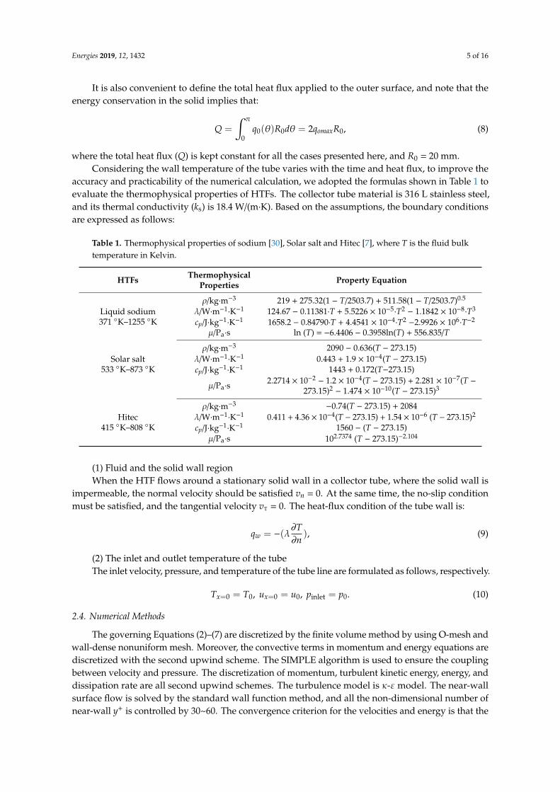
The heat-flux distributions on the whole absorber outer wall (case 1) are consistent with the result of Equation (1) shown in Figure 5.

Figure 5. 3D heat-flux distribution on the outer tube’s wall.

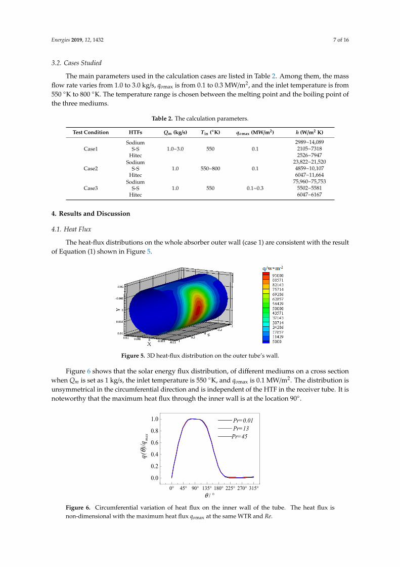
Figure 6 shows that the solar energy flux distribution, of different mediums on a cross section when Qm is set as 1 kg/s, the inlet temperature is 550 °K, and qomax is 0.1 MW/m2. The distribution is unsymmetrical in the circumferential direction and is independent of the HTF in the receiver tube. It is noteworthy that the maximum heat flux through the inner wall is at the location 90°.

0° 45° 90° 135° 180° 225° 270° 315°

0.0

0.2

0.4

0.6

0.8

1.0

q(θ)

/qm

ax

Pr=0.01 Pr=13Pr=45

θ / °

Figure 6. Circumferential variation of heat flux on the inner wall of the tube. The heat flux is non-dimensional with the maximum heat flux qomax at the same WTR and Re.

Figure 5. 3D heat-flux distribution on the outer tube’s wall.

Figure 6 shows that the solar energy flux distribution, of different mediums on a cross sectionwhen Qm is set as 1 kg/s, the inlet temperature is 550 ◦K, and qomax is 0.1 MW/m2. The distribution isunsymmetrical in the circumferential direction and is independent of the HTF in the receiver tube. It isnoteworthy that the maximum heat flux through the inner wall is at the location 90◦.

Energies 2019, 12, x FOR PEER REVIEW 7 of 16

550 °K to 800 °K. The temperature range is chosen between the melting point and the boiling point of the three mediums.

Table 2. The calculation parameters.

Test condition HTFs Qm (kg/s) Tin (°K) qomax (MW/m2) h (W/m2 K)

Case1 Sodium

S-S Hitec

1.0 ~ 3.0 550 0.1 2989~14089 2105~7318 2526~7947

Case2 Sodium

S-S Hitec

1.0 550 ~ 800 0.1 23822~21520 4859~10107 6047~11664

Case3 Sodium

S-S Hitec

1.0 550 0.1 ~ 0.3 75960~75753 5502~5581 6047~6167

4. Results and Discussion

4.1. Heat Flux

The heat-flux distributions on the whole absorber outer wall (case 1) are consistent with the result of Equation (1) shown in Figure 5.

Figure 5. 3D heat-flux distribution on the outer tube’s wall.

Figure 6 shows that the solar energy flux distribution, of different mediums on a cross section when Qm is set as 1 kg/s, the inlet temperature is 550 °K, and qomax is 0.1 MW/m2. The distribution is unsymmetrical in the circumferential direction and is independent of the HTF in the receiver tube. It is noteworthy that the maximum heat flux through the inner wall is at the location 90°.

0° 45° 90° 135° 180° 225° 270° 315°

0.0

0.2

0.4

0.6

0.8

1.0

q(θ)

/qm

ax

Pr=0.01 Pr=13Pr=45

θ / °

Figure 6. Circumferential variation of heat flux on the inner wall of the tube. The heat flux is non-dimensional with the maximum heat flux qomax at the same WTR and Re.

Figure 6. Circumferential variation of heat flux on the inner wall of the tube. The heat flux isnon-dimensional with the maximum heat flux qomax at the same WTR and Re.

Energies 2019, 12, 1432 8 of 16

4.2. Temperature Profile

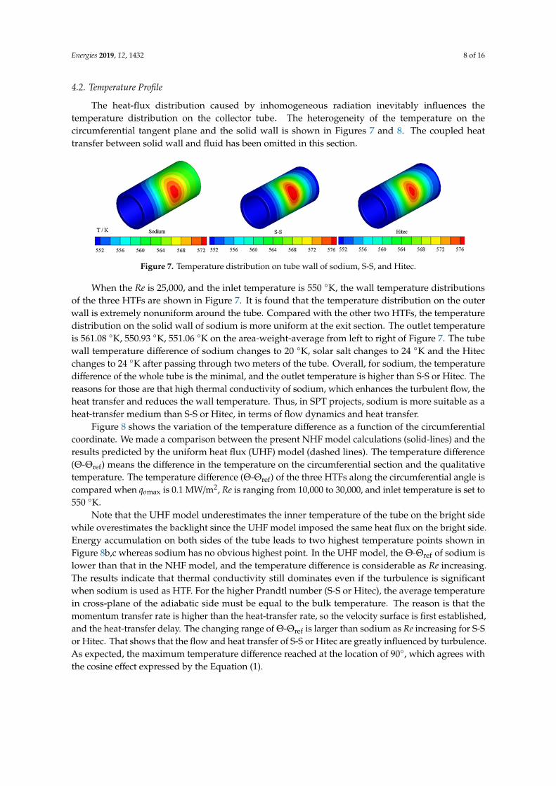
The heat-flux distribution caused by inhomogeneous radiation inevitably influences thetemperature distribution on the collector tube. The heterogeneity of the temperature on thecircumferential tangent plane and the solid wall is shown in Figures 7 and 8. The coupled heattransfer between solid wall and fluid has been omitted in this section.

Energies 2019, 12, x FOR PEER REVIEW 8 of 16

4.2. Temperature Profile

The heat-flux distribution caused by inhomogeneous radiation inevitably influences the temperature distribution on the collector tube. The heterogeneity of the temperature on the circumferential tangent plane and the solid wall is shown in Figure (7)–(8). The coupled heat transfer between solid wall and fluid has been omitted in this section.

When the Re is 25,000, and the inlet temperature is 550 °K, the wall temperature distributions of the three HTFs are shown in Figure 7. It is found that the temperature distribution on the outer wall is extremely nonuniform around the tube. Compared with the other two HTFs, the temperature distribution on the solid wall of sodium is more uniform at the exit section. The outlet temperature is 561.08 °K, 550.93 °K, 551.06 °K on the area-weight-average from left to right of Figure 7. The tube wall temperature difference of sodium changes to 20 °K, solar salt changes to 24 °K and the Hitec changes to 24 °K after passing through two meters of the tube. Overall, for sodium, the temperature difference of the whole tube is the minimal, and the outlet temperature is higher than S-S or Hitec. The reasons for those are that high thermal conductivity of sodium, which enhances the turbulent flow, the heat transfer and reduces the wall temperature. Thus, in SPT projects, sodium is more suitable as a heat-transfer medium than S-S or Hitec, in terms of flow dynamics and heat transfer.

Figure 7. Temperature distribution on tube wall of sodium, S-S, and Hitec.

Figure 8 shows the variation of the temperature difference as a function of the circumferential coordinate. We made a comparison between the present NHF model calculations (solid-lines) and the results predicted by the uniform heat flux (UHF) model (dashed lines). The temperature difference (Θ-Θref) means the difference in the temperature on the circumferential section and the qualitative temperature. The temperature difference (Θ-Θref) of the three HTFs along the circumferential angle is compared when qomax is 0.1 MW/m2, Re is ranging from 10,000 to 30,000, and inlet temperature is set to 550 °K.

Note that the UHF model underestimates the inner temperature of the tube on the bright side while overestimates the backlight since the UHF model imposed the same heat flux on the bright side. Energy accumulation on both sides of the tube leads to two highest temperature points shown in Figure 8(b)–(c) whereas sodium has no obvious highest point. In the UHF model, the Θ-Θref of sodium is lower than that in the NHF model, and the temperature difference is considerable as Re increasing. The results indicate that thermal conductivity still dominates even if the turbulence is significant when sodium is used as HTF. For the higher Prandtl number (S-S or Hitec), the average temperature in cross-plane of the adiabatic side must be equal to the bulk temperature. The reason is that the momentum transfer rate is higher than the heat-transfer rate, so the velocity surface is first established, and the heat-transfer delay. The changing range of Θ-Θref is larger than sodium as Re increasing for S-S or Hitec. That shows that the flow and heat transfer of S-S or Hitec are greatly influenced by turbulence. As expected, the maximum temperature difference reached at the location of 90°, which agrees with the cosine effect expressed by the Equation (1).

Figure 7. Temperature distribution on tube wall of sodium, S-S, and Hitec.

When the Re is 25,000, and the inlet temperature is 550 ◦K, the wall temperature distributionsof the three HTFs are shown in Figure 7. It is found that the temperature distribution on the outerwall is extremely nonuniform around the tube. Compared with the other two HTFs, the temperaturedistribution on the solid wall of sodium is more uniform at the exit section. The outlet temperatureis 561.08 ◦K, 550.93 ◦K, 551.06 ◦K on the area-weight-average from left to right of Figure 7. The tubewall temperature difference of sodium changes to 20 ◦K, solar salt changes to 24 ◦K and the Hitecchanges to 24 ◦K after passing through two meters of the tube. Overall, for sodium, the temperaturedifference of the whole tube is the minimal, and the outlet temperature is higher than S-S or Hitec. Thereasons for those are that high thermal conductivity of sodium, which enhances the turbulent flow, theheat transfer and reduces the wall temperature. Thus, in SPT projects, sodium is more suitable as aheat-transfer medium than S-S or Hitec, in terms of flow dynamics and heat transfer.

Figure 8 shows the variation of the temperature difference as a function of the circumferentialcoordinate. We made a comparison between the present NHF model calculations (solid-lines) and theresults predicted by the uniform heat flux (UHF) model (dashed lines). The temperature difference(Θ-Θref) means the difference in the temperature on the circumferential section and the qualitativetemperature. The temperature difference (Θ-Θref) of the three HTFs along the circumferential angle iscompared when qomax is 0.1 MW/m2, Re is ranging from 10,000 to 30,000, and inlet temperature is set to550 ◦K.

Note that the UHF model underestimates the inner temperature of the tube on the bright sidewhile overestimates the backlight since the UHF model imposed the same heat flux on the bright side.Energy accumulation on both sides of the tube leads to two highest temperature points shown inFigure 8b,c whereas sodium has no obvious highest point. In the UHF model, the Θ-Θref of sodium islower than that in the NHF model, and the temperature difference is considerable as Re increasing.The results indicate that thermal conductivity still dominates even if the turbulence is significantwhen sodium is used as HTF. For the higher Prandtl number (S-S or Hitec), the average temperaturein cross-plane of the adiabatic side must be equal to the bulk temperature. The reason is that themomentum transfer rate is higher than the heat-transfer rate, so the velocity surface is first established,and the heat-transfer delay. The changing range of Θ-Θref is larger than sodium as Re increasing for S-Sor Hitec. That shows that the flow and heat transfer of S-S or Hitec are greatly influenced by turbulence.As expected, the maximum temperature difference reached at the location of 90◦, which agrees withthe cosine effect expressed by the Equation (1).

Energies 2019, 12, 1432 9 of 16Energies 2019, 12, x FOR PEER REVIEW 9 of 16

315°270°225°180°135°90°0°

1.0

0.5

0.0

-0.5

NHF-10000 UHF-10000 NHF-12000 UHF-12000 NHF-15000 UHF-15000 NHF-16500 UHF-16500 NHF-20000 UHF-20000 NHF-25000 UHF-25000 NHF-30000 UHF-30000

Θ−Θ

ref/K

θ / °

-1.045°

(a) Liquid sodium

0.0

0.5

1.0

1.5

2.0

180° 315°270°225°135°90°45°

NHF-10000 UHF-10000 NHF-12000 UHF-12000 NHF-15000 UHF-15000 NHF-16500 UHF-16500 NHF-20000 UHF-20000 NHF-25000 UHF-25000 NHF-30000 UHF-30000

Θ−Θ

ref /

K

θ / °0°

(b) Solar salt

0° 45° 90° 135° 180° 225° 270° 315°

0.00.20.40.60.81.01.21.4

θ / °

Θ−Θ

ref/K

NHF-10000 UHF-10000 NHF-12000 UHF-12000 NHF-15000 UHF-15000 NHF-16500 UHF-16500 NHF-20000 UHF-20000 NHF-25000 UHF-25000 NHF-30000 UHF-30000

(c) Hitec

Figure 8. (a–c) Circumferential variation of the inner wall fluid temperature with the qualitative temperature for different Reynolds number at a fixed-inlet temperature (Tin=550 °K ). (a) Pr=0.001 (b) Pr=13 (c) Pr=50. Solid lines: the present calculations; Dashed lines: homogeneous heat-flux model (HHFM).

The value of Θ-Θref is slightly dependent on the Re but strongly affected by the Pr. In general, the Θ-Θref is increasing as the Pr increases, decreasing as the Re increases. Comparing Figure 8(a–c), the temperature difference of S-S at the location θ = 90° is 1.93 times higher than sodium, and Hitec is 1.35 times higher that of sodium when Re is 10,000. The temperature difference of S-S is 1.29 times higher than sodium, and Hitec is 2.0 times sodium when Re is 30,000. The results reflect that sodium has a good effect on solving the uneven temperature caused by nonuniform heat flux, which may reduce the risk of hot spots and, thus, reduce pipe stresses.

Figure 8. (a–c) Circumferential variation of the inner wall fluid temperature with the qualitativetemperature for different Reynolds number at a fixed-inlet temperature (Tin = 550 ◦K). (a) Pr = 0.001(b) Pr = 13 (c) Pr = 50. Solid lines: the present calculations; Dashed lines: homogeneous heat-fluxmodel (HHFM).

The value of Θ-Θref is slightly dependent on the Re but strongly affected by the Pr. In general, theΘ-Θref is increasing as the Pr increases, decreasing as the Re increases. Comparing Figure 8a–c, thetemperature difference of S-S at the location θ = 90◦ is 1.93 times higher than sodium, and Hitec is 1.35times higher that of sodium when Re is 10,000. The temperature difference of S-S is 1.29 times higherthan sodium, and Hitec is 2.0 times sodium when Re is 30,000. The results reflect that sodium has agood effect on solving the uneven temperature caused by nonuniform heat flux, which may reduce therisk of hot spots and, thus, reduce pipe stresses.

Energies 2019, 12, 1432 10 of 16

Another concern is the inner wall temperature, also called film temperature, which could leadto the degradation of the HTFs. The inner wall temperature distribution in NHF and UHF modelsare shown in Figure 9a–c when Re is 25,000, and the inlet temperature is 550 K. From Figure 9a–c, theaverage temperature of the fluid in the tube is: 562.8 ◦K, 554.9 ◦K, 554.7 ◦K. Figure 9a–c show that oneof the most significant advantages of sodium over S-S and Hitec is that the temperature distribution ismuch more uniform on both the inner and outer surface of the tube.Energies 2019, 12, x FOR PEER REVIEW 10 of 16

(a) (d)

(b) (e)

(c) (f)

Figure 9. (a–c) Temperature distribution of three kinds of media under two models and (d–e) velocity distribution under NHF model.

Another concern is the inner wall temperature, also called film temperature, which could lead to the degradation of the HTFs. The inner wall temperature distribution in NHF and UHF models are shown in Figure 9(a)–(c) when Re is 25,000, and the inlet temperature is 550 K. From Figure 9(a) to (c), the average temperature of the fluid in the tube is: 562.8 °K, 554.9 °K, 554.7 °K. Figure 9(a)–(c) show that one of the most significant advantages of sodium over S-S and Hitec is that the temperature distribution is much more uniform on both the inner and outer surface of the tube.

Obviously, for the NHF model, there is a heat spot on the outer wall from 0° to 180°, especially at 90°. At the same time, the UHF model is idealistic. But, the highest heat spot temperature of sodium is the lowest, while S-S and Hitec are same. There is a considerable temperature gradient when the sodium flows in the receiver tube. Besides, not far from the entrance, the inner fluid temperature is higher and more uniform than S-S or Hitec flow in the tube.

Corresponding velocity distribution is shown in Figure 9(e)–(f). The velocity of sodium is the lowest, only 0.19 times the other two mediums. At a distance of 0.2 m from the inlet, the sodium flow reached fully developed, and the boundary layer is thinner, while the other boundary conditions

Sodium-NHF Sodium-UHF

45°

90°135°

45°

90°135°

0°0°

45°

90°135°

45°90°

135°

0°0°

Hitec-NHF Hitec-UHF

Figure 9. (a–c) Temperature distribution of three kinds of media under two models and (d,e) velocitydistribution under NHF model.

Obviously, for the NHF model, there is a heat spot on the outer wall from 0◦ to 180◦, especially at90◦. At the same time, the UHF model is idealistic. But, the highest heat spot temperature of sodiumis the lowest, while S-S and Hitec are same. There is a considerable temperature gradient when thesodium flows in the receiver tube. Besides, not far from the entrance, the inner fluid temperature ishigher and more uniform than S-S or Hitec flow in the tube.

Energies 2019, 12, 1432 11 of 16

Corresponding velocity distribution is shown in Figure 9e,f. The velocity of sodium is the lowest,only 0.19 times the other two mediums. At a distance of 0.2 m from the inlet, the sodium flow reachedfully developed, and the boundary layer is thinner, while the other boundary conditions remainedunchanged. It can be explained that the molecule heat conduction of sodium dominates in fullydeveloped turbulent heat transfer. The heat diffusion of the medium with lower Prandtl number(sodium) is much higher than the momentum transfer diffusivity.

4.3. Effects of Mass Flow

Figure 10 shows the dependence of h, f of the three HTFs on Qm, which varies from 0.2 to 1.4 kg/s.The values of maximum heat flux and inlet temperature are set to 0.1 MW/m2 and 550 ◦K, respectively.

Energies 2019, 12, x FOR PEER REVIEW 11 of 16

remained unchanged. It can be explained that the molecule heat conduction of sodium dominates in fully developed turbulent heat transfer. The heat diffusion of the medium with lower Prandtl number (sodium) is much higher than the momentum transfer diffusivity.

4.3. Effects of Mass Flow

Figure 10 shows the dependence of h, f of the three HTFs on Qm, which varies from 0.2 to 1.4 kg/s. The values of maximum heat flux and inlet temperature are set to 0.1 MW/m2 and 550 °K, respectively.

0.2 0.4 0.6 0.8 1.0 1.2 1.4

14,000

12,000

10,000

8000

6000

4000

h (w

/m2 ⋅k

)

Qm

/(Kg/s)

Sodium Hitec S-S

2000

0.2 0.4 0.6 0.8 1.0 1.2 1.4

0.020.030.040.050.060.070.080.09

f

Qm/(kg/s)

Sodium Hitec SS

Pres

sure

Dro

p(Δp

)/Pa16

12

8

4

Sodium Hitec SS

0

×104

(a) (b)

Figure 10. Effects of Qm on the heat-transfer performance of the HTFs in the tube: (a) Qm-h, (b) Qm-f-Δp.

The average heat-transfer coefficient of all working fluids increases with the mass flow. When the Qm increases by 0.3 kg/s, the h of S-S, Hitec and sodium increases by an average of 1303, 1355, 2775 W/m2･°K, respectively. The variation of Qm has a significant influence on the heat-transfer characteristic of the HTFs, especially on sodium. For sodium, the higher the Qm, the better the heat-transfer coefficient. The reason is that the average temperature difference is getting smaller increasingly with the rise of Qm when the maximum heat flux is 0.1 MW/m2. However, the law of change in the average friction coefficient is reversed, all decreasing as the flow rate increases. When the Qm is higher than 0.8 kg/s, the friction coefficient decreases slowly. S-S and Hitec, with high heat-transfer rate and low-pressure drop, are exceptionally beneficial for heat transfer. The results suggest that the Qm should be higher than 0.8 kg/s to obtain greater heat-transfer performance. However, a larger mass-flow rate represents more considerable pump pressure and more substantial heat absorption capability. Besides, without increasing the solar thermal input, it is possible to cause the reduction of fluid temperature and increase the corresponding heat loss.

4.4. Effects of Inlet Temperature

The physical properties of the HTF are primarily affected by the inlet temperature (Tin). The typical operating temperatures for the three HTFs are shown in Table 3. The available temperature range is between the melting point and the boiling point. The trends of h, f for the three HTFs have been shown in Figure 11. Tin is varying from 550 °K to 800 °K, Qm is 1.0 kg/s, and qomax is 0.1 MW/m2.

Table 3. Comparison of the physical properties for different HTFs proposed for CRS applications. The physical properties are evaluated at 550 °K, 1 bar. melting point = m.p, normal boiling point (n.b.p). Sources: [35–37].

Candidate HTF

m.p °K

n.b.p °K

ρCp kJ/m3·°K

Sodium 371 1255 1166 Solar salt 533 873 2498

Figure 10. Effects of Qm on the heat-transfer performance of the HTFs in the tube: (a) Qm-h, (b) Qm-f -∆p.

The average heat-transfer coefficient of all working fluids increases with the mass flow. Whenthe Qm increases by 0.3 kg/s, the h of S-S, Hitec and sodium increases by an average of 1303, 1355,2775 W/m2

·◦K, respectively. The variation of Qm has a significant influence on the heat-transfer

characteristic of the HTFs, especially on sodium. For sodium, the higher the Qm, the better theheat-transfer coefficient. The reason is that the average temperature difference is getting smallerincreasingly with the rise of Qm when the maximum heat flux is 0.1 MW/m2. However, the law ofchange in the average friction coefficient is reversed, all decreasing as the flow rate increases. When theQm is higher than 0.8 kg/s, the friction coefficient decreases slowly. S-S and Hitec, with high heat-transferrate and low-pressure drop, are exceptionally beneficial for heat transfer. The results suggest thatthe Qm should be higher than 0.8 kg/s to obtain greater heat-transfer performance. However, a largermass-flow rate represents more considerable pump pressure and more substantial heat absorptioncapability. Besides, without increasing the solar thermal input, it is possible to cause the reduction offluid temperature and increase the corresponding heat loss.

4.4. Effects of Inlet Temperature

The physical properties of the HTF are primarily affected by the inlet temperature (Tin). Thetypical operating temperatures for the three HTFs are shown in Table 3. The available temperaturerange is between the melting point and the boiling point. The trends of h, f for the three HTFs havebeen shown in Figure 11. Tin is varying from 550 ◦K to 800 ◦K, Qm is 1.0 kg/s, and qomax is 0.1 MW/m2.

From Figure 11a, the heat-transfer coefficient of sodium is larger by about 2.5 to 5 times than theother two kinds of molten salt and decreases slowly with the temperature rising. The reason for theabove unique heat-transfer feature of sodium is its high conductivity, and it decreases with increasingtemperature even in turbulent flow. As shown in Figure 11c, the conductivity of sodium is 118, 154times Hitec and S-S at 550 ◦K, respectively. Furthermore, the h of Hitec or S-S increases linearly with theincrease of temperature whereas sodium is the opposite. The h of Hitec has not changed significantly

Energies 2019, 12, 1432 12 of 16

between 750 ◦K and 800 ◦K because its boiling point is 808 ◦K. The greater the h, the smaller the f whenthe mass-flow rate is constant for the three HTFs. Besides, from Table 3, the energy-storage capacity(ρCp) of Hitec or S-S is two times more than the sodium.

Table 3. Comparison of the physical properties for different HTFs proposed for CRS applications. Thephysical properties are evaluated at 550 ◦K, 1 bar. melting point = m.p, normal boiling point (n.b.p).Sources: [35–37].

Candidate HTF m.p◦K

n.b.p◦K

ρCp

kJ/m3·◦K

Sodium 371 1255 1166Solar salt 533 873 2498

Hitec 415 808 2411

Energies 2019, 12, x FOR PEER REVIEW 12 of 16

Hitec 415 808 2411 From Figure 11(a), the heat-transfer coefficient of sodium is larger by about 2.5 to 5 times than

the other two kinds of molten salt and decreases slowly with the temperature rising. The reason for the above unique heat-transfer feature of sodium is its high conductivity, and it decreases with increasing temperature even in turbulent flow. As shown in Figure 11(c), the conductivity of sodium is 118, 154 times Hitec and S-S at 550 °K, respectively. Furthermore, the h of Hitec or S-S increases linearly with the increase of temperature whereas sodium is the opposite. The h of Hitec has not changed significantly between 750 °K and 800 °K because its boiling point is 808 °K. The greater the h, the smaller the f when the mass-flow rate is constant for the three HTFs. Besides, from Table 3, the energy-storage capacity (ρCp) of Hitec or S-S is two times more than the sodium.

Based on the above conclusions, we can select sodium as the heat-transfer medium in the collector tube on the top of the SPT, while the Hitec or S-S as the circulating medium or storage medium, respectively.

550 600 650 700 750 800

30,000

25,000

20,000

15,000

10,000

h (W

/m2 ⋅k

)

T / K

Sodium Hitec S-S

5000

550 600 650 700 750 800

0.012

0.016

0.020

0.024

0.028

f

T / K

Sodium Hitec SS

(a) (b)

550 600 650 700 750 800

800

1000

1200

1400

1600

1800

2000

ρ/(k

g·m

- ³)

T / K

SS Hitec Sodium

0.000

0.001

0.002

0.003

0.004

SS Hitec Sodium

μ/(P

a·S)

0

20

40

60

80

100

SS Hitec Sodium

λ/(W

·m-2

k-1)

1000

1100

1200

1300

1400

1500

1600

SS Hitec Sodium

Cp/(J

·Kg-1

K-1

)

(c)

Figure 11. Effects of Tin on the performance of tube: (a) T-h; (b) T-f; (c) T-ρ-μ-Cp-λ.

4.5 Effects of Heat Flux on the Outside Surface

Generally, the heat flux on the outside surfaces of the receiver tubes in SPT plants is quite limited to give a reasonable lifetime. The maximum heat flux allowed (allowable flux density), qomax, has progressively grown for many years, such as 0.35 MW/m2 in the Solar One plant and 0.8 MW/m2 in the Solar Two plant. Besides, the qomax is a crucial parameter for the receiver design, since it is directly related to the heliostat field cost, which involves the number of heliostats and the arrangement strategy [38,39].

Figure 11. Effects of Tin on the performance of tube: (a) T-h; (b) T-f ; (c) T-ρ-µ-Cp-λ.

Based on the above conclusions, we can select sodium as the heat-transfer medium in thecollector tube on the top of the SPT, while the Hitec or S-S as the circulating medium or storagemedium, respectively.

Energies 2019, 12, 1432 13 of 16

4.5. Effects of Heat Flux on the Outside Surface

Generally, the heat flux on the outside surfaces of the receiver tubes in SPT plants is quite limitedto give a reasonable lifetime. The maximum heat flux allowed (allowable flux density), qomax, hasprogressively grown for many years, such as 0.35 MW/m2 in the Solar One plant and 0.8 MW/m2

in the Solar Two plant. Besides, the qomax is a crucial parameter for the receiver design, since it isdirectly related to the heliostat field cost, which involves the number of heliostats and the arrangementstrategy [38,39].

Figure 12a,b show the variations of h, f of the three HTFs when qomax varies from 0.1 to 0.3 MW/m2.The values of mass flow rate and inlet temperature are set to 1.0 kg/s and 550 ◦K, respectively. Theincreased maximum heat flux does not affect the average heat-transfer coefficient of HTFs in the tube,and the h of sodium is invariably 12.56 times that of Hitec and 13.8 times that of S-S. At the same time,the flow of liquid sodium in the tube maintains a small friction coefficient compared to the other twoworking fluids (Figure 12b). Therefore, liquid sodium ensures economics while maintaining efficientsystem operation.

Energies 2019, 12, x FOR PEER REVIEW 13 of 16

Figure 12(a) and (b) show the variations of h, f of the three HTFs when qomax varies from 0.1 to 0.3 MW/m2. The values of mass flow rate and inlet temperature are set to 1.0 kg/s and 550 °K, respectively. The increased maximum heat flux does not affect the average heat-transfer coefficient of HTFs in the tube, and the h of sodium is invariably 12.56 times that of Hitec and 13.8 times that of S-S. At the same time, the flow of liquid sodium in the tube maintains a small friction coefficient compared to the other two working fluids (Figure 12(b)). Therefore, liquid sodium ensures economics while maintaining efficient system operation.

As shown in Figure 12(c) and (d), when the maximum heat flux changed from 0.1 to 0.3 MW/m2, the temperature of the outer wall increased from 554.53 °K to 563.61 °K while the average temperature of the circumferential increased by about 2 °K. At the same time, the temperature difference between the inner and outer walls is smaller than 4 °K in both cases. As a result, the thermal stress acting on the heat-transfer tubes is greatly reduced.

h (W

/m2 ⋅k

)

×1053.02.01.5 2.5

8.0

6.0

4.0

qomax / (W⋅m-2)

Sodium Hitec S-S

2.0

×104

1.0

0.016

0.020

0.024

0.028f

Sodium Hitec SS

×1053.02.01.5 2.5

qomax / (W⋅m-2)1.0

(a) (b)

qmax =0.1 MW/m2 qmax = 0.3 MW/m2

(c) (d)

Figure 12. Effects of qomax: (a) qomax-h, (b) qomax-f, (c–d) qomax-T.

5. Conclusions

The heat-transfer characteristic of liquid sodium is compared with solar salt and Hitec in a heat-transfer tube for the SPT system. The calculations present the effects of operational parameters (Qm, Tin, qomax) on the thermal and thermo-hydraulic performance of three mediums under a nonuniform heat flux. The following conclusions are obtained:

(a) The tube wall temperature difference of sodium is 20 °K, which is 4 °K lower than other the two mediums when the Re is 25,000, and the inlet temperature is 550 °K. In either NHF model or UHF model, the temperature distribution of Sodium is more uniform and higher than S-S and Hitec, and the highest temperature on the hot spot is 4 °K lower than S-S or Hitec.

(b) Among these factors (Qm, Tin, qomax), the change of Qm has an essential influence on the heat-transfer coefficient of HTFs. However, even in high turbulence, the thermal conductivity of Sodium still plays a crucial role. Meanwhile, the change of qomax does not affect the average heat-transfer performance of the heat-transfer medium, but it has a significant influence on the

Figure 12. Effects of qomax: (a) qomax-h, (b) qomax-f, (c,d) qomax-T.

As shown in Figure 12c,d, when the maximum heat flux changed from 0.1 to 0.3 MW/m2, thetemperature of the outer wall increased from 554.53 ◦K to 563.61 ◦K while the average temperature ofthe circumferential increased by about 2 ◦K. At the same time, the temperature difference between theinner and outer walls is smaller than 4 ◦K in both cases. As a result, the thermal stress acting on theheat-transfer tubes is greatly reduced.

Energies 2019, 12, 1432 14 of 16

5. Conclusions

The heat-transfer characteristic of liquid sodium is compared with solar salt and Hitec in aheat-transfer tube for the SPT system. The calculations present the effects of operational parameters(Qm, Tin, qomax) on the thermal and thermo-hydraulic performance of three mediums under anonuniform heat flux. The following conclusions are obtained:

(a) The tube wall temperature difference of sodium is 20 ◦K, which is 4 ◦K lower than other thetwo mediums when the Re is 25,000, and the inlet temperature is 550 ◦K. In either NHF model or UHFmodel, the temperature distribution of Sodium is more uniform and higher than S-S and Hitec, and thehighest temperature on the hot spot is 4 ◦K lower than S-S or Hitec.

(b) Among these factors (Qm, Tin, qomax), the change of Qm has an essential influence on theheat-transfer coefficient of HTFs. However, even in high turbulence, the thermal conductivity of Sodiumstill plays a crucial role. Meanwhile, the change of qomax does not affect the average heat-transferperformance of the heat-transfer medium, but it has a significant influence on the temperature of thetube wall. Loading excessively high heat flux on the collector tube may cause many security issues inSPT system.

(c) Under the same boundary conditions, the heat-transfer performance of Sodium is one order ofmagnitude higher than that of S-S and Hitec at low temperature (550 ◦K~700 ◦K), and it is twice thanthe two kinds of molten salts at high temperature (700 ◦K +).

Author Contributions: Conceptualization, Y.H.; Data curation, J.L.; Formal analysis, J.L.; Funding acquisition,Y.H.; Investigation, J.L.; Methodology, Y.H. and X.L.; Validation, J.L.; Writing—original draft, J.L.; Writing—review& editing, J.L., Y.H. and X.L.

Funding: This work was funded by the National Natural Science Foundation of China (grant number 50876090).

Conflicts of Interest: The authors declare no conflict of interest.

References

1. Sargent and Lundy LLC Consulting Group. Assessment of Parabolic Trough and Power Tower Solar TechnologyCost and Performance Forecasts; Report No. NREL/SR-550-34440; NREL: Golden, CO, USA, 2003. [CrossRef]

2. García-Barberena, J.; Monreal, A.; Mutuberria, A.; Sánchez, M. Towards cost-competitive solartowers—Energy cost reductions based on decoupled solar combined cycles (DSCC). Energy Procedia 2014, 49,1350–1360. [CrossRef]

3. Hinkley, J.; Curtin, B.; Hayward, J.; Wonhas, A.; Boyd, R.; Grima, C.; Tadros, A.; Hall, R.; Naicker, K.;Mikhail, A. Concentrating Solar Power—Drivers and Opportunities for Cost-Competitive Electricity; Report No.EP111647; CSIRO: Canberra, Australia, 2011. [CrossRef]

4. Roldán, M.I.; Monterreal, R. Heat flux and temperature prediction on a volumetric receiver installed in asolar furnace. Appl. Energy 2014, 120, 65–74. [CrossRef]

5. Chang, C.; Li, X.; Zhang, Q.Q. Experimental and Numerical Study of the Heat Transfer Characteristics inSolar Thermal Absorber Tubes with Circumferentially Non-uniform Heat Flux. Energy Procedia 2014, 49,305–313. [CrossRef]

6. Romero, M.; González-Aguilar, J. Next generation of liquid metal and other high-performance receiverdesigns for concentrating solar thermal (CST) central tower systems. Adv. Conc. Sol. Therm. Res. Technol.2017, 129–154. [CrossRef]

7. Siegel, N.P.; Bradshaw, R.W.; Cordaro, J.B.; Kruizenga, A.M. Thermophysical property measurement ofnitrate salt heat transfer fluids. In Proceedings of the ASME 2011 5th International Conference on EnergySustainability, Washington, DC, USA, 7–10 August 2011; pp. 439–446. [CrossRef]

8. Pacio, J.; Singer, C.; Wetzel, T.; Uhlig, R. Thermodynamic evaluation of liquid metals as heat transfer fluids inconcentrated solar power plants. Appl. Therm. Eng. 2013, 60, 295–302. [CrossRef]

9. Kearney, D.; Herrmann, U.; Nava, P.; Kelly, B.; Mahoney, R.; Pacheco, J.; Cable, R.; Potrovitza, N.; Blake, D.;Price, H. Assessment of a molten salt heat transfer fluid in a parabolic trough solar field. J. Sol. Energy Eng.2003, 125, 170–176. [CrossRef]

Energies 2019, 12, 1432 15 of 16

10. Thomas, W.; Julio, P.; Luca, M.; Alfons, W.; Annette, H.; Wolfgang, H.; Carsten, S.; Georg, M.; Jürgen, K.;Robert, S.; et al. Liquid metal technology for concentrated solar power systems: Contributions by theGerman research program. AIMS Energy 2014, 2, 89–98. [CrossRef]

11. Guidez, J.; Martin, L.; Chetal, S.; Chellapandi, P.; Raj, B. Lessons learned from sodium-cooled fast reactoroperation and their ramifications for future reactors with respect to enhanced safety and reliability.Nucl. Technol. 2008, 164, 207–220. [CrossRef]

12. Singer, C.; Buck, R.; Pitz-Paal, R.; Müller-Steinhagen, H. Assessment of solar power tower drivenultrasupercritical steam cycles applying tubular central receivers with varied heat transfer media. J. Sol.Energy Eng. 2010, 132, 41010. [CrossRef]

13. Hering, W.; Stieglitz, R.; Wetzel, T. Application of liquid metals for solar energy systems. EPJ Web ofConferences. EDP Sci. 2012, 33, 03003. [CrossRef]

14. Bienert, W.B. The heat pipe and its application to solar receivers. Electr. Power Syst. Res. 1980, 3, 111–123.[CrossRef]

15. Boerema, N.; Morrison, G.; Taylor, R.; Rosengarten, G. Liquid sodium versus Hitec as a heat transfer fluid insolar thermal central receiver systems. Sol. Energy 2012, 86, 2293–2305. [CrossRef]

16. Kotzé, J.P.; von Backström, T.W.; Erens, P.J. NaK as a primary heat transfer fluid in thermal solar powerinstallations. In Proceedings of the SolarPACES 2012 International Conference, Durban, South Africa,27–29 March 2014.

17. Amy, C.; Budenstein, D.; Bagepalli, M.; England, D.; Deangelis, F.; Wilk, G.; Jarrett, C.; Kelsall, C.; Hirschey, J.;Wen, H.; et al. Pumping liquid metal at high temperatures up to 1,673 kelvin. Nature 2017, 550, 199–203.[CrossRef] [PubMed]

18. DeAngelis, F.; Seyf, H.R.; Berman, R.; Schmidt, G.; Moore, D.; Henry, A. Design of a high temperature(1350 ◦C) solar receiver based on a liquid metal heat transfer fluid: Sensitivity analysis. Sol. Energy 2018, 164,200–209. [CrossRef]

19. Pacio, J.; Wetzel, T. Assessment of liquid metal technology status and research paths for their use as efficientheat transfer fluids in solar central receiver systems. Sol. Energy 2013, 93, 11–22. [CrossRef]

20. Pacio, J.; Fritsch, A.; Singer, C.; Uhlig, R. Liquid metals as efficient coolants for high-intensity point-focusreceivers: Implications to the design and performance of next-generation CSP systems. Energy Procedia 2014,49, 647–655. [CrossRef]

21. Matsubara, K.; Sakurai, A.; Miura, T.; Kawabata, T. Spanwise heat transport in turbulent channel flow withPrandtl numbers ranging from 0.025 to 5.0. J. Heat Transf. 2012, 134, 041701. [CrossRef]

22. Flores, O.; Marugán-Cruz, C.; Santana, D.; Garcia-Villalba, M. Thermal stresses analysis of a circular tube ina central receiver. Int. Conf. Sol. PACES 2014, 49, 354–362. [CrossRef]

23. Rodríguez-Sánchez, M.; Venegas-Bernal, M.; Marugán-Cruz, C.; Santana, D. Thermal, mechanical andhydrodynamic analysis to optimize the design of molten salt central receivers of solar tower power plants.In Proceedings of the International Conference on Renewable Energies and Power Quality (ICREPQ’13),Bilbao, Spain, 20–22 March 2013; pp. 128–133. [CrossRef]

24. Irfan, M.A.; Chapman, W. Thermal stresses in radiant tubes due to axial, circumferential and radialtemperature distributions. Appl. Therm. Eng. 2009, 29, 1913–1920. [CrossRef]

25. Fritsch, A.; Uhlig, R.; Marocco, L.; Frantz, C.; Flesch, R.; Hoffschmidt, B. A comparison between transientCFD and FEM simulations of solar central receiver tubes using molten salt and liquid metals. Sol. Energy2017, 155, 259–266. [CrossRef]

26. Flesch, J.; Niedermeier, K.; Fritsch, A.; Musaeva, D.; Marocco, L.; Uhlig, R.; Baake, E.; Buck, R.; Wetzel, T.Liquid metals for solar power systems. IOP Conf. Ser. Mater. Sci. Eng. 2017, 228, 012012. [CrossRef]

27. Gartshore, I.; Salcudean, M.; Hassan, I. Film cooling injection hole geometry: Hole shape comparison forcompound cooling orientation. AIAA J. 2015, 39, 1493–1499. [CrossRef]

28. Rodríguez-Sánchez, M.R.; Soria-Verdugo, A.; Almendros-Ibáñez, J.A.; Acosta-Ibáñez, A.; Santana, D. Thermaldesign guidelines of solar power towers. Appl. Therm. Eng. 2014, 63, 428–438. [CrossRef]

29. Patankar, S. Numerical Heat Transfer and Fluid Flow; Hemisphere Publishing: Washington, DC, USA, 1980.30. Mikityuk, K. Heat transfer to liquid metal: Review of data and correlations for tube bundles. Nucl. Eng. Des.

2009, 239, 680–687. [CrossRef]31. Minkowycz, W.J.; Sparrow, E.M.; Murthy, J.Y. Handbook of Numerical Heat Transfer, 2nd ed.; John Wiley &

Sons: New York, NY, USA, 2000.

Energies 2019, 12, 1432 16 of 16

32. Wu, M.; Li, M.; Xu, C.; He, Y.L.; Tao, W.Q. The impact of concrete structure on the thermal performance ofthe dual-media thermocline thermal storage tank using concrete as the solid medium. Appl. Energy 2014,113, 1363–1371. [CrossRef]

33. He, Y.L.; Tao, W.Q. Convective heat transfer enhancement: Mechanisms, techniques, and performanceevaluation. Adv. Heat Transf. 2014, 46, 87–186. [CrossRef]

34. Gnielinski, V. New equations for heat and mass transfer in turbulent pipe and channel flow. Int. Chem. Eng.1976, 16, 8–16.

35. Zavoico, A.B. Solar Power Tower Design Basis Document, Revision 0; Report of Sandia National Laboratories:San Francisco, CA, USA, 2001. [CrossRef]

36. Foust, O.J. Sodium-NaK Engineering Handbook; Gordon and Breach Science Publishers: New York, NY, USA,1972; pp. 32–38.

37. VDI-Gesellschaft Verfahrenstechnik und Chemieingenieurwesen (GVC). VDI Heat Atlas, 2nd. ed.; Springer:Berlin, Germany, 2010.

38. Vant-Hull, L.L. The role of “allowable flux density” in the design and operation of molten-salt solar centralreceivers. J. Sol. Energy Eng. 2002, 124, 165–169. [CrossRef]

39. Liao, Z.; Li, X.; Xu, C.; Chang, C.; Wang, Z. Allowable flux density on a solar central receiver. Renew. Energ.2014, 62, 747–753. [CrossRef]

© 2019 by the authors. Licensee MDPI, Basel, Switzerland. This article is an open accessarticle distributed under the terms and conditions of the Creative Commons Attribution(CC BY) license (http://creativecommons.org/licenses/by/4.0/).