Heat transfer coefficients from Newtonian and non-Newtonian fluids flowing

in laminar regime in a helical coil

T.A. Pimenta, J.B.L.M. Campos

ABS T RA CT

This study aimed to carry out experimental work to obtain, for Newtonian and non-Newtonian fluids, heat transfer coefficients, at constant wall

temperature as boundary condition, in fully developed laminar flow inside a helical coil. The Newtonian fluids studied were aqueous solutions of glycerol,

25%, 36%, 43%, 59% and 78% (w/w) and the non-Newtonian fluids aqueous solutions of carboxymethylcellulose (CMC), a polymer, with concentrations

0.1%, 0.2%, 0.3%, 0.4% and 0.6% (w/w) and aqueous solutions of xanthan gum (XG), another polymer, with concentrations 0.1% and 0.2% (w/w).

According to the rheological study performed, the polymer solutions had shear thinning behavior and different values of elasticity. The heli- cal coil used

has internal diameter, curvature ratio, length and pitch, respectively: 0.004575 m, 0.0263,

5.0 m and 11.34 mm. The Nusselt numbers for the CMC solutions are, on average, slightly higher than those for Newtonian fluids, for identical Prandtl

and generalized Dean numbers. As outcome, the viscous component of the shear thinning polymer tends to potentiate the mixing effect of the Dean

cells. The Nusselt numbers of the XG solutions are significant lower than those of the Newtonian solutions, for identical Prandtl and generalized

Dean numbers. Therefore, the elastic component of the polymer tends to diminish the mixing effect of the Dean cells. A global correlation, for Nusselt

number as a function of Péclet, generalized Dean and Weissenberg numbers for all Newtonian and non-Newtonian solutions studied, is presented.

K eyw ords Helical coil, Heat transfer coefficients, Newtonian fluids, Non-Newtonian fluids, Viscoelasticity, Laminar flow

1. Introduction

Coiled tubes of helical shape are widely used as heat exchangers

and have multiple applications in various industries: chemical, bio-

logical, petrochemical, biomedical among others. In these indus-

tries, they are applied in a large range of processes, such as:

sterilization, pasteurization, concentration, crystallization, separa-

tion (distillation) and reaction. They are also found in general pur-

pose equipment: refrigeration, air conditioning and water heating.

The fluids involved in these processes may have Newtonian or non-

Newtonian behavior.

The helical coils are widely used because they have large heat

transfer areas, they are compact, and, above all, their geometry

promotes a good mixing of the fluids, increasing the heat and mass

transfer coefficients. In addition, this equipment has low cost and

is of easy construction and maintenance.

The mixing characteristics are consequence of the development

of secondary flows along the tube, the so called Dean effect (Dean

[1]). These secondary flows appear due to the centrifugal force act-

ing on the fluid elements. The difference in axial velocity among

the fluid elements flowing in a cross-section leads to a centrifugal

gradient. The elements flowing in the center are projected, under

the centrifugal force, into the outer wall direction of the coil, where

they suffer a decrease of velocity. Afterwards, they return to the

center of the tube, forming two, for the case of tubes with a circular

cross-section, counter-rotation vortices, the so called Dean cells

(Dean [1]). This flow pattern promotes the mixture of the fluid ele-

ments. Studies have shown that these secondary flows still have a

stabilizing effect on the global flow, promoting a higher critical

Reynolds number for transition from laminar to turbulent than

that in a straight tube. The secondary flow enhances also the heat

transfer in curved pipes in comparison to straight pipes, i.e., the

heat transfer coefficients from the coil to the flowing fluid are high-

er than those in a straight pipe, for the same flow conditions and

Prandtl number.

Many authors studied, theoretically and experimentally, heat

transfer in coils for Newtonian fluids, among them: Mori and

Nakayama [2–4], Schmidt [5], Dravid et al. [6], Akiyama and Cheng

[7,8], Tarbell and Samuels [9], Kalb and Seader [10], Olivier and Asg-

har [11], Janssen and Hoogendoorn [12], Manlapaz and Churchill

G0

G00

Nomenclature

Ai internal lateral area of the coil tube (m2)

Amln mean logarithmic lateral area of the coil tube (m2)

Ao external lateral area of the coil tube (m2)

aT shift factor

Cp mean heat specific capacity of the fluid (J kg-1 K-1)

Cpwater mean heat specific capacity of the water (J kg-1 K-1)

Cpsyst mean heat specific capacity of the system (oil, coil and

Tw internal wall temperature of the coil (°C)

UA global heat transfer coefficient from the oil to the fluid

(solutions of glycerol, CMC and XG) in the coil times

the lateral area of the coil (W K-1)

(UA)losses global heat transfer coefficient from the oil to the ambi-

ent air times the internal area of the tank (W K-1)

v mean flow velocity of the fluid (m s-1) tank) (J kg-1 K-1)

dc coil diameter (m)

dc/di curvature of the coil

di inside tube diameter (m)

G0 storage module (Pa)

G00 loss module (Pa)

r reduced storage module (Pa)

r reduced loss module (Pa)

V_ volumetric flow of the fluid flowing inside the coil

(m3 s-1)

xcoil wall thickness of the tube coil (m)

DH activation energy for flow (Jmol-1)

DP pressure drop of the fluid in the coil (Pa)

DTln logarithmic mean temperature difference (°C)

Greek symbols

hic heat transfer film coefficient between the inner wall of

the coil and the fluid flowing in the coil (W m2 K-1) c_ shear rate (s-1)

c_ r reduced shear rate (s-1)

hoc

kcopper

heat transfer film coefficient between the oil and the

outer wall of the coil (W m2 K-1)

thermal conductivity of the copper (W m K-1)

g viscometric viscosity (Pa s)

go viscometric viscosity at zero shear rate (Pa s)

gr reduced viscometric viscosity (Pa s)

kf thermal conductivity of the fluid (W m K-1) k relaxation time (s)

Kw

K

consistency index of the fluid calculated at wall temper-

ature (Tw) (Pa sn)

consistency index of the fluid for a given temperature

(Pa sn)

q density (kg m-3)

qref density at Tref (kg m-3)

x angular frequency (s-1)

xr reduced angular frequency (s-1) Lcoil length of the coil (m) m minimum Dimensionless numbers M maximum De Dean number msyst

m_ m_ water

N1

mass of oil, coil and tank (kg)

mass flow of the fluid flowing inside the coil (kg s-1)

mass flow of water inside the coil (kg s-1)

first normal tress difference (kg m-1 s-2)

De(g) modified Dean number

El elasticity number

Eu Euler number

Gz Graetz number

n power-law index of the fluid (index of behavior) He helical number

nt

p Q_

R

number of turns of the coil

pitch of the coil (m)

heat power (W)

ideal gas constant ((Jmol-1 K-1)

Nuc Nusselt number for a fluid in a coil

Nus Nusselt number for a fluid in a straight tube

Pe Péclet number

Pr Prandtl number

t T

time (s)

temperature (K) Pr(g) modified Prandtl number

Pr⁄ Prandtl number (used by Hsu and Patankar [19]) Tamb

tdef

Te

ambient temperature (°C) characteristic time of the flow (s)

inlet temperature of the fluid in the coil (°C)

Pr(N) Prandtl number (used by Nigam et al. [20])

(Pr)w Prandtl number at wall temperature of the tube

Re Reynolds number

Tf

Tle

mean film temperature of the fluid (°C) external surface temperature of the lateral wall of the

Rec critical Reynolds number Wi Weissenber gnumber

agitation tank (°C) Tli internal surface temperature of the lateral wall of the Acronyms

agitation tank (°C) CMC carboxymethylcellulose

Tm mean temperature of the fluid (bulk temperature) (°C) MXEC modified Xin and Ebadian correlation Toil bulk oil temperature (°C) PAA polyacrylamide Tref reference temperature (K) SAOS small amplitude oscillatory shear tests

Ts exit temperature of the coil (°C) w/w percentage by weight Tte external surface temperature of the top wall of the XG xanthan gum

agitation tank (°C) Tti internal surface temperature of the top wall of the

agitation tank (°C)

[13], Xin and Ebadian [14] and Jayakumar et al. [15,16]. The great

majority of these studies are theoretical, complemented with

numerical methods and applied to tubes with zero pitch geometry.

The published studies about heat transfer coefficients for non-

Newtonian fluids flowing inside coils are still scarce. From a liter-

ature review, we stand out the following works: Rajasekharan et al.

[17,18], Olivier and Asghar [11], Hsu and Patankar [19] and Nigam

et al. [20]. The majority of these authors concluded that, for the

same flow conditions and Prandtl number, shear thinning fluids

have smaller heat transfer coefficients than Newtonian fluids,

while shear thickening fluids have higher. The study of the elastic

effect of the fluids on the heat transfer coefficients in helical coils is

still very incipient.

The motivation of the present study is to contribute to the yet

incipient study of non-Newtonian fluids, in particular, to the anal-

ysis of the elastic effect in the heat transfer coefficients in helical

Table 1

Literature for Nusselt number correlations applied to Newtonian fluids.

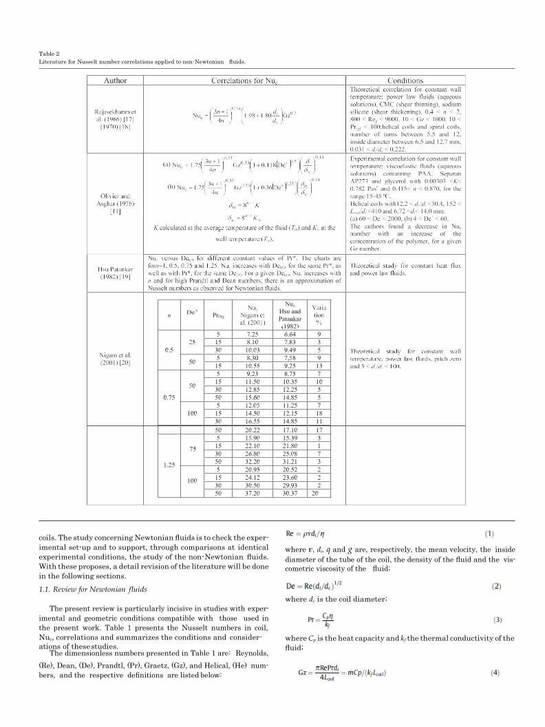
Table 2

Literature for Nusselt number correlations applied to non-Newtonian fluids.

coils. The study concerning Newtonian fluids is to check the exper-

imental set-up and to support, through comparisons at identical

experimental conditions, the study of the non-Newtonian fluids.

With these proposes, a detail revision of the literature will be done

in the following sections.

where v, di, q and g are, respectively, the mean velocity, the inside

diameter of the tube of the coil, the density of the fluid and the vis-

cometric viscosity of the fluid;

1.1. Review for Newtonian fluids

The present review is particularly incisive in studies with exper-

imental and geometric conditions compatible with those used in

the present work. Table 1 presents the Nusselt numbers in coil,

where dc is the coil diameter;

Nuc, correlations and summarizes the conditions and consider-

ations of these studies. The dimensionless numbers presented in Table 1 are: Reynolds,

where Cp is the heat capacity and kf the thermal conductivity of the

fluid;

(Re), Dean, (De), Prandtl, (Pr), Graetz, (Gz), and Helical, (He) num-

bers, and the respective definitions are listed below:

where Lcoil is the length of the coil and m_ the mass flow of the fluid

and the product RePr the Péclet number, Pe;

i

where p is the pitch of the coil.

1.2. Review for non-Newtonian fluids

The correlations chronologically listed in Table 2 allow the cal-

culation of Nusselt number in coil, Nuc, for laminar flow and fully

developed non-Newtonian fluids, with the viscometric component

following the power law. These studies are, as referred above,

scarce. -

The dimensionless numbers used in Table 2 are:

- generalized Reynolds number (Reg) (Metzner and Reed [21]): -

Reg ¼

where K is the consistency index and n the behavior index of the

fluid.

Table 3

Dimensions of the helical coil of copper.

Average of the measured

values

Internal diameter of the coil (mm) 167.79 ± 1.21

External coil diameter (mm) 179.47 ± 1.27

Coil height (mm) 111.11 ± 0.85

Vertical distance between turns (mm) 4.99 ± 0.09

2. Experimental work

2.1. Experimental set-up

Table 3 presents the dimensions of the copper coil used in this

study and the respective uncertainties. Fig. 1 shows a flow diagram Angle of the turns with the horizontal plane

(°) 3.17 ± 0.19 of the experimental set-up employed to determine the heat trans-

Inside diameter of the tube (mm) 4.32 ± 0.05

External diameter of the tube (mm) 6.35 ± 0.05

Internal diameter of the fittings (mm) 4.01 ± 0.03

Length of the coil tube (m) 5.5 ± 3.79

Coil pitch (mm) 11.34

Number of turns 9.4

fer coefficients, for the condition of constant wall temperature. The

fluid circulated in a close loop from a first tank, where the temper-

ature was controlled and set constant at 20 °C by means of a heat

pump and a refrigerator, to inside the copper coil. The coil was sub-

merged in a bath of oil mechanically agitated placed in another

tank as depicted in Fig. 1. This tank was thermally isolated and

Fig. 1. Scheme of the experimental set-up. The temperature meters are: Toil for the oil temperature; Te and Ts for the fluid at the entrance and exit of the coil, respectively; Tw

for the wall temperature of the coil; Tle and Tli for the external and internal surface of the lateral wall of the tank, respectively; Tte and Tti for the external and internal surface of

the top wall of the tank, respectively; Tamb for the ambient temperature. dP represents the pressure transducer used to measure the pressure drop of the fluid inside the helical

coil. A heat pump and a refrigerator were used to maintain constant the temperature of the fluid at the coil inlet. A temperature controller was used to maintain the oil at

constant temperature. The electromagnetic flowmeter measured the fluid flow rate.

was provided with a heating system and a temperature controller.

The experimental set-up had a centrifugal pump, a transducer to

measure the pressure drop of the fluid inside the helical coil

(uncertainty 0.028% full scale (0–6 bar)), an electromagnetic flow-

meter (uncertainty of 1.2% of the volumetric flow), several ther-

mometers T type and Pt100 type (maximum uncertainty of

1.3 °C) and two data acquisition systems (a OMEGA PCI 1602 sys-

tem with 16 bit of resolution for the transducer and electromag-

netic flowmeter and a Validyne UPC601-T system with 14 bit of

resolution for the temperature meters).

The oil, where the coil was immersed, was a mineral oil used for

heat transfer proposes, and it was accompanied by a technical

sheet specifying the physical properties.

The heat transfer boundary condition was constant wall tem-

perature (Tw) due to the high rotational velocity of the stirrer

(1100 min-1) and, by consequence, to the low heat transfer resis-

tance from the bath to the internal wall of the coil. This boundary

condition was validated comparing temperatures measured at the

wall of the coil (two positions) and at the oil bath. The relative dif-

ference was never higher than 4%.

The experimental rig was validated calculating, with experi-

mental data, both sides of the energy balance equation applied to

the cooling of the bath, by water flowing in the coil, in unsteady

conditions:

between 80 and 30 °C. The relative uncertainty of these experi-

ments is 4.76%.

2.2. Characterization of the fluids

The Newtonian fluids were aqueous solutions of glycerol of 25%,

36%, 43%, 59% and 78% (w/w) and the non-Newtonian fluids aque-

ous solutions of carboxymethylcellulose (CMC) of 0.1%, 0.2%, 0.3%,

1.4 % and 0.6% (w/w), with molar mass 3 x 105 kg kmol-1(grade

7H4C from Hercules), and aqueous solutions of xanthan gum

(XG) of 0.1% and 0.2% (w/w), with molar mass 2 x 106 kg kmol-1

(grade G1253 from Sigma-Aldrich).The values of the physical prop-

erties of the glycerol solutions were obtained in the literature and

the viscosity of the solutions was experimentally obtained in a

rotational viscometer. The physical properties of the non-Newto-

nian solutions, except the rheological properties, were taken as

identical to those of pure water (Pinho and Coelho [22], Rohsenow

et al. [23] and Semmar et al. [24]).

2.2.1. Rheological characterization of the non-Newtonian fluids

The viscous and elastic components of the non-Newtonian solu-

tions were characterized in a cutting edge rheometer, trademark

PHYSICA model MCR301, and the geometry used was that of

cone-plate. The viscometric viscosity was determined, as a func-

tion of the shear rate, through steady state shear tests and the elas-

tic component through first normal stress difference, N1, and through the loss (G00 ) and storage (G0 ) modules, these obtained in

where (UA)losses(Toil - Tamb) represents the heat flux lost to the ambi-

ent air.

oscillation tests (small amplitude oscillatory shear tests (SAOS)).

For the elastic component, tests in a capillary break-up rheometer,

trademark Haake CaBER 1 Thermo Scientific, were also performed. The rheological tests were performed at 20, 25, 30, 35, 40 and

Previously, the global heat transfer coefficient from the oil to 45 °C, according to the range of the mean temperature (T ) of the ambient air ((UA)losses) was experimentally determined, in un-

steady state experiments: the oil was heated until a pre-defined

temperature and, afterwards, was cooled by the ambient air, i.e.,

without any cooling fluid flowing inside the coil.

Fig. 2 shows the results of the experimental rig validation.

m

the fluids flowing in the coil. To have additional rheological data,

between these temperatures, it was applied the method of reduced

variables, described by Bird et al. [25]. In this method, one of the

experimental data curve is chosen to be the master curve (data at a temperature designated, from now on, by reference tempera-

To obtain the film heat transfer coefficient from the oil to the ture, T ). The factor that allows the overlapping of the other curves coil, hoc = f (Toil), some experiments were performed, also in

unsteady conditions. The experiments were similar to those de-

scribed above, but, this time, with water at high flow rates flowing

inside the coil. In these flow conditions, the dominant thermal

resistance was that between the oil and the wall, i.e., any increase in the water flow rate did not induce any effect in the overall heat

ref

with the master curve is called the shift factor, aT. For each concen-

tration, this shift factor is function of the temperature and is calcu-

lated, supposing negligible effect of the temperature in the density,

by:

transfer coefficient. For each experiment, the oil was cooling

where go is the viscometric viscosity at zero shear rate for temper-

atures T and Tref, respectively.

According to Bird et al. [25], the shift factor is related with the

temperature by Arrhenius equation:

where DH is the activation energy and R the ideal gas constant.

According to the reduced variables method, the reduced shear

rate, c_ r , is given by:

and, once more supposing the density of the solutions independent

of the temperature, the reduced viscometric viscosity, gr, is given

by:

Fig. 2. Results of the experimental energy balance, Eq. (14), for rig validation; the

solid line is at 45°.

According to Metzner and Reed [21], for fluids that follow the power

law, the reduced viscometric viscosity is given by:

r

r

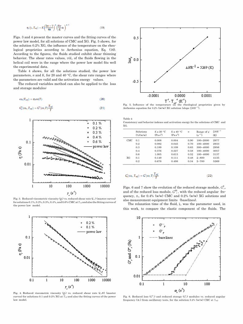
Figs. 3 and 4 present the master curves and the fitting curves of the

power law model, for all solutions of CMC and XG. Fig. 5 shows, for

the solution 0.2% XG, the influence of the temperature on the rheo-

logical proprieties according to Arrhenius equation, Eq. (16).

According to the figures, the fluids studied exhibit shear thinning

behavior. The shear rates values, v/di, of the fluids flowing in the

helical coil were in the range where the power law model fits well

the experimental data.

Table 4 shows, for all the solutions studied, the power law

parameters, n and K, for 20 and 40 °C, the shear rate ranges where

the parameters are valid and the activation energy values.

The reduced variables method can also be applied to the loss

and storage modules:

Fig. 5. Influence of the temperature on the rheological proprieties given by

Arrhenius equation for 0.2% (w/w) XG solution (slope DHR-1).

Table 4

Consistency and behavior indexes and activation energy for the solutions of CMC and

XG.

Solutions

(%)(w/w)

K a 20 °C

(Pa sn)

K a 40 °C

(Pa sn)

n Range of c_

(s-1

)

DHR-1

(K)

CMC 0.1 0.008 0.004 0.90 100–2000 2977

0.2 0.082 0.045 0.70 100–4000 2933

0.3 0.189 0.109 0.63 300–4000 2956

0.4 0.376 0.227 0.58 100–4000 3057

0.6 1.005 0.615 0.52 100–4000 3137

XG 0.1 0.149 0.111 0.48 2–800 4135

0.2 0.678 0.498 0.34 2–700 5269

G0 0

r

Fig. 3. Reduced viscometric viscosity (gr) vs. reduced shear rate (c_ r ) (master curves)

for solutions 0.1%, 0.2%, 0.3%, 0.4%, and 0.6% CMC at Tref and also the fitting curves of

the power law model.

Figs. 6 and 7 show the evolution of the reduced storage module, G0 ,

and of the reduced loss module, G00 , with the reduced angular fre-

quency, xr, for 0.4% (w/w) CMC and 0.2% (w/w) XG solutions and

also measurement equipment limits (baselines).

The relaxation time of the fluid, k, was the parameter used, in

this work, to compare the elastic component of the fluids. The

Fig. 4. Reduced viscometric viscosity (gr) vs. reduced shear rate (c_ r Þ) (master

curves) for solutions 0.1 and 0.2% XG at Tref and also the fitting curves of the power

law model.

Fig. 6. Reduced loss (G0 0 r) and reduced storage (G0

r) modules vs. reduced angular

frequency (xr) from oscillatory tests, for the solution 0.4% (w/w) CMC at Tref.

of the solutions. Furthermore the relaxation times obtained with

CaBER method are between 30 and 200 times lower than those ob-

tained by SAOS method. Coelho and Pinho [26] used the same car-

boxymethylcellulose (CMC) with identical solute concentrations,

0.1%, 0.2%, 0.3% and 0.4% (w/w) and performed creep tests to deter-

mine the relaxation times. Comparing their results with the pres-

ent results obtained by SAOS method (Table 5), it can be

observed a good accordance. Like Cavadas et al. [27] it was found

a large dispersion on results of the first normal stress difference

(N1).

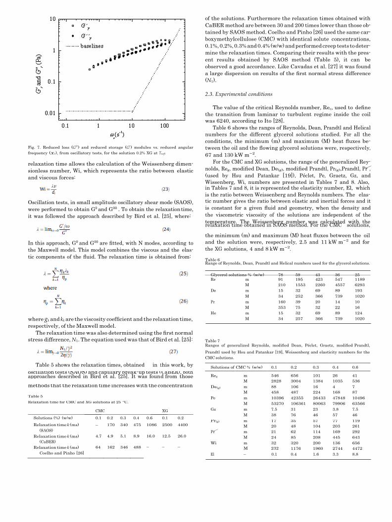
2.3. Experimental conditions

Fig. 7. Reduced loss (G0 0 ) and reduced storage (G0 ) modules vs. reduced angular

frequency (xr), from oscillatory tests, for the solution 0.2% XG at Tref.

relaxation time allows the calculation of the Weissenberg dimen-

sionless number, Wi, which represents the ratio between elastic

and viscous forces:

The value of the critical Reynolds number, Rec, used to define

the transition from laminar to turbulent regime inside the coil

was 6240, according to Ito [28].

Table 6 shows the ranges of Reynolds, Dean, Prandtl and Helical

numbers for the different glycerol solutions studied. For all the

conditions, the minimum (m) and maximum (M) heat fluxes be-

tween the oil and the flowing glycerol solutions were, respectively,

67 and 130 kW m-2.

For the CMC and XG solutions, the range of the generalized Rey-

nolds, Reg, modified Dean, De(g), modified Prandtl, Pr(g),Prandtl, Pr⁄,

(used by Hsu and Patankar [19]), Péclet, Pe, Graetz, Gz, and

Wissenberg, Wi, numbers are presented in Tables 7 and 8. Also,

in Tables 7 and 8, it is represented the elasticity number, El, which

is the ratio between Weissenberg and Reynolds numbers. The elas-

Oscillation tests, in small amplitude oscillatory shear mode (SAOS),

were performed to obtain G0 and G00 . To obtain the relaxation time,

it was followed the approach described by Bird et al. [25], where:

tic number gives the ratio between elastic and inertial forces and it

is constant for a given fluid and geometry, when the density and

the viscometric viscosity of the solutions are independent of the

temperature. The Weissenberg number was calculated with the relaxation time obtained in SAOS method. For the CMC solutions,

the minimum (m) and maximum (M) heat fluxes between the oil

In this approach, G0 and G00 are fitted, with N modes, according to

the Maxwell model. This model combines the viscous and the elas-

tic components of the fluid. The relaxation time is obtained from:

and the solution were, respectively, 2.5 and 11 kW m-2 and for

the XG solutions, 4 and 8 kW m-2.

Table 6 Range of Reynolds, Dean, Prandtl and Helical numbers used for the glycerol solutions.

Glycerol solutions % (w/w) 78 59 43 36 25

where gk and kk are the viscosity coefficient and the relaxation time,

respectively, of the Maxwell model.

The relaxation time was also determined using the first normal

stress difference, N1. The equation used was that of Bird et al. [25]:

Table 7 Ranges of generalized Reynolds, modified Dean, Péclet, Graetz, modified Prandtl,

Prandtl used by Hsu and Patankar [19], Weissenberg and elasticity numbers for the

CMC solutions.

Table 5 shows the relaxation times, obtained in this work, by Solutions of CMC % (w/w) 0.1 0.2 0.3 0.4 0.6

oscillation tests (SAOS) and capillary break-up tests ( approaches described in Bird et al. [25]. It was foun

CaBER), both d from those Reg m 546 656 101 26 41

M 2828 3004 1384 1035 536

methods that the relaxation time increases with the concentration De(g) m 88 106 16 4 7

M 458 487 224 168 87 Table 5

Pe m 10396 42355 26433 47848 10496 Relaxation time for CMC and XG solutions at 25 °C.

M 53270 106361 80063 79906 63566

CMC XG Gz m 7.5 31 23 3.8 7.5

Solutions (%) (w/w) 0.1 0.2 0.3 0.4 0.6

0.1 0.2 M 38 76 46 57 46

Relaxation time k (ms) – 170 340 475 1086 2500 4400 Pr(g) m

M

17

20

35

48

57

104

77

203

119

261 (SAOS) Pr

⁄ m 21 62 114 169 292

Relaxation time k (ms) 4.7 4.9 5.1 8.9 16.0 12.5 26.0 M 24 85 208 445 643 (CaBER) Wi m 32 320 200 136 656

Relaxation time k (ms) 64 162 346 488 – – – M 232 1176 1960 2744 4472 Coelho and Pinho [26] El – 0.1 0.4 1.6 3.3 8.8

Re m 91 195 423 547 1189

M 210 1553 2260 4557 6293

De m 15 32 69 89 193

M 34 252 366 739 1020

Pr m 160 39 20 14 10

M 353 75 32 22 16

He m 15 32 69 89 124

M 34 257 366 739 1020

p

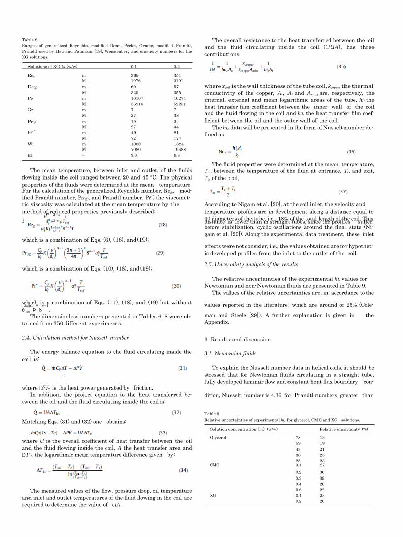
Table 8

Ranges of generalized Reynolds, modified Dean, Péclet, Graetz, modified Prandtl,

Prandtl used by Hsu and Patankar [19], Weissenberg and elasticity numbers for the

XG solutions.

The overall resistance to the heat transferred between the oil

and the fluid circulating inside the coil (1/UA), has three

contributions:

Solutions of XG % (w/w) 0.1 0.2

Reg m 369 351

M 1976 2191

De(g) m 60 57

M 320 355

Pe m 10107 10274

M 36916 52251

Gz m 7 7

M 27 38

Pr(g) m 19 24

M 27 44

Pr⁄

m 49 81

M 72 177

Wi m 1000 1824

where xcoil is the wall thickness of the tube coil, kcopper the thermal

conductivity of the copper, Ai , Ao and Am ln are, respectively, the

internal, external and mean logarithmic areas of the tube, hic the

heat transfer film coefficient between the inner wall of the coil

and the fluid flowing in the coil and hoc the heat transfer film coef-

ficient between the oil and the outer wall of the coil.

The hic data will be presented in the form of Nusselt number de-

fined as

M 7080 19688

El – 3.6 9.8

The mean temperature, between inlet and outlet, of the fluids

flowing inside the coil ranged between 20 and 45 °C. The physical

properties of the fluids were determined at the mean temperature.

The fluid properties were determined at the mean temperature,

Tm, between the temperature of the fluid at entrance, Te, and exit,

Ts, of the coil,

For the calculation of the generalized Reynolds number, Reg, mod-

ified Prandtl number, Pr(g), and Prandtl number, Pr⁄, the viscomet-

ric viscosity was calculated at the mean temperature by the

method of reduced properties previously described: dn 2-n T

According to Nigam et al. [20], at the coil inlet, the velocity and

temperature profiles are in development along a distance equal to

30 diameters of the tube, i.e., 18% of the total length of the coil. This Reg ¼ i v q ref n 1þ3n n 8n-1T distance is lower than in straight tubes, since the profiles suffer,

which is a combination of Eqs. (6), (18), and (19);

before stabilization, cyclic oscillations around the final state (Ni-

gam et al. [20]). Along the experimental data treatment, these inlet

effects were not consider, i.e., the values obtained are for hypothet-

ic developed profiles from the inlet to the outlet of the coil.

which is a combination of Eqs. (10), (18), and (19); 2.5. Uncertainty analysis of the results

The relative uncertainties of the experimental hic values for

Newtonian and non-Newtonian fluids are presented in Table 9.

which is a combination of Eqs. (11), (18), and (19) but without

The values of the relative uncertainties are, in, accordance to the

3nþ1 n n-1 values reported in the literature, which are around of 25% (Cole- ð 4n Þ 8 .

The dimensionless numbers presented in Tables 6–8 were ob-

tained from 350 different experiments.

2.4. Calculation method for Nusselt number

The energy balance equation to the fluid circulating inside the

coil is:

man and Steele [29]). A further explanation is given in the

Appendix.

3. Results and discussion

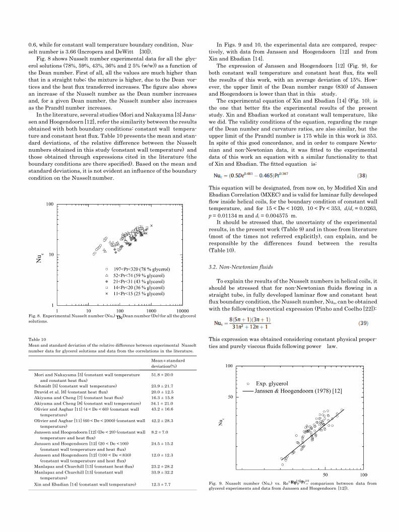
3.1. Newtonian fluids

where DPV_ is the heat power generated by friction.

To explain the Nusselt number data in helical coils, it should be

stressed that for Newtonian fluids circulating in a straight tube,

fully developed laminar flow and constant heat flux boundary con-

In addition, the project equation to the heat transferred be-

tween the oil and the fluid circulating inside the coil is:

Matching Eqs. (31) and (32) one obtains:

where U is the overall coefficient of heat transfer between the oil

and the fluid flowing inside the coil, A the heat transfer area and

DTln the logarithmic mean temperature difference given by:

dition, Nusselt number is 4.36 for Prandtl numbers greater than

Table 9

Relative uncertainties of experimental hic for glycerol, CMC and XG solutions.

Solution concentration (%) (w/w) Relative uncertainty (%)

Glycerol 78 13

59 19

43 21

36 25

25 23 CMC 0.1 27

0.2 36

0.3 39

0.4 20

The measured values of the flow, pressure drop, oil temperature

and inlet and outlet temperatures of the fluid flowing in the coil are

required to determine the value of UA.

0.6 22

XG 0.1 23

0.2 20

0.6, while for constant wall temperature boundary condition, Nus-

selt number is 3.66 (Incropera and DeWitt [30]).

Fig. 8 shows Nusselt number experimental data for all the glyc-

erol solutions (78%, 59%, 43%, 36% and 2 5% (w/w)) as a function of

the Dean number. First of all, all the values are much higher than

that in a straight tube; the mixture is higher, due to the Dean vor-

tices and the heat flux transferred increases. The figure also shows

an increase of the Nusselt number as the Dean number increases

and, for a given Dean number, the Nusselt number also increases

as the Prandtl number increases.

In the literature, several studies (Mori and Nakayama [3] Jans-

sen and Hoogendoorn [12], refer the similarity between the results

obtained with both boundary conditions: constant wall tempera-

ture and constant heat flux. Table 10 presents the mean and stan-

dard deviations, of the relative difference between the Nusselt

numbers obtained in this study (constant wall temperature) and

those obtained through expressions cited in the literature (the

boundary conditions are there specified). Based on the mean and

standard deviations, it is not evident an influence of the boundary

condition on the Nusselt number.

In Figs. 9 and 10, the experimental data are compared, respec-

tively, with data from Janssen and Hoogendoorn [12] and from

Xin and Ebadian [14].

The expression of Janssen and Hoogendoorn [12] (Fig. 9), for

both constant wall temperature and constant heat flux, fits well

the results of this work, with an average deviation of 15%. How-

ever, the upper limit of the Dean number range (830) of Janssen

and Hoogendoorn is lower than that in this study.

The experimental equation of Xin and Ebadian [14] (Fig. 10), is

the one that better fits the experimental results of the present

study. Xin and Ebadian worked at constant wall temperature, like

we did. The validity conditions of the equation, regarding the range

of the Dean number and curvature ratios, are also similar, but the

upper limit of the Prandtl number is 175 while in this work is 353.

In spite of this good concordance, and in order to compare Newto-

nian and non-Newtonian data, it was fitted to the experimental

data of this work an equation with a similar functionality to that

of Xin and Ebadian. The fitted equation is:

This equation will be designated, from now on, by Modified Xin and

Ebadian Correlation (MXEC) and is valid for laminar fully developed

flow inside helical coils, for the boundary condition of constant wall

temperature, and for 15 < De < 1020, 10 < Pr < 353, di/dc = 0.0263,

p = 0.01134 m and di = 0.004575 m.

It should be stressed that, the uncertainty of the experimental

results, in the present work (Table 9) and in those from literature

(most of the times not referred explicitly), can explain, and be

responsible by the differences found between the results

(Table 10).

3.2. Non-Newtonian fluids

To explain the results of the Nusselt numbers in helical coils, it

should be stressed that for non-Newtonian fluids flowing in a

straight tube, in fully developed laminar flow and constant heat

flux boundary condition, the Nusselt number, Nus, can be obtained

with the following theoretical expression (Pinho and Coelho [22]):

Fig. 8. Experimental Nusselt number (Nuc) vs. Dean number (De) for all the glycerol

solutions.

Table 10

Mean and standard deviation of the relative difference between experimental Nusselt

number data for glycerol solutions and data from the correlations in the literature.

This expression was obtained considering constant physical proper-

ties and purely viscous fluids following power law.

Mori and Nakayama [3] (constant wall temperature

and constant heat flux)

Mean ± standard

deviation(%)

51.8 ± 20.0

Schmidt [5] (constant wall temperature) 23.9 ± 21.7

Dravid et al. [6] (constant heat flux) 20.0 ± 12.5

Akiyama and Cheng [7] (constant heat flux) 16.3 ± 15.8

Akiyama and Cheng [8] (constant wall temperature) 34.1 ± 21.0

Olivier and Asghar [11] (4 < De < 60) (constant wall

temperature)

Olivier and Asghar [11] (60 < De < 2000) (constant wall

temperature)

Janssen and Hoogendoorn [12] (De < 20) (constant wall

temperature and heat flux)

Janssen and Hoogendoorn [12] (20 < De < 100)

(constant wall temperature and heat flux)

Janssen and Hoogendoorn [12] (100 < De < 830)

(constant wall temperature and heat flux)

43.2 ± 16.6

42.2 ± 28.3

8.2 ± 7.0

24.5 ± 15.2

12.0 ± 12.3

Manlapaz and Churchill [13] (constant heat flux) 23.2 ± 28.2

Manlapaz and Churchill [13] (constant wall

temperature)

33.9 ± 32.2

Xin and Ebadian [14] (constant wall temperature) 12.3 ± 7.7 Fig. 9. Nusselt number (Nuc) vs. Re0.43

Pr1/6

– comparison between data from

glycerol experiments and data from Janssen and Hoogendoorn [12]).

Fig. 10. Nusselt number (Nuc) vs. Dean number (De) – comparison between data

from glycerol experiments and data from Xin and Ebadian [14]).

Fig. 11. Nusselt number (Nuc) vs. Dean number (De(g)) for the non-Newtonian

fluids CMC and XG experiments – comparison between experimental data and

results obtained from correlation for glycerol solutions (MXEC).

For the condition of constant wall temperature, once more

according to Pinho and Coelho [22], the values are 3.66, 3.95,

4.18 and 5.80 respectively for the behavior index of, 1, 0.5, 0.33

and 0.

For both boundary conditions, the greater is the behavior index,

the lower is the Nusselt number. For a straight tube, the literature

states that the results presented for both boundary conditions are

valid either for purely viscous fluids as for viscoelastic fluids (Pinho

and Coelho [22]).

Rajasekharan et al. [17,18], Olivier and Asghar [11], Hsu and

Patankar [19] and Nigam et al. [20]) performed studies with non-

Newtonian fluids, for similar conditions to those used in this work.

Hsu and Patankar [19] studied theoretically the heat transfer for

fluids that follow the power law, for the boundary condition of

constant heat flux. These authors found that for the same Dean

number (De(g)) and Prandtl number (Pr⁄), the Nusselt numbers

for shear thinning fluids are lower than those for Newtonian fluids.

In order to confirm this statement, it was represented the Nusselt

number as a function of the generalized Dean number, as shown in

Fig. 11. The Nusselt numbers for the glycerol solutions were ob-

tained from equation MXEC. It can be seen, with the help of Ta-

ble 11, that for the same ranges of Prandtl (Pr⁄) and Dean (De(g))

numbers, the Nusselt numbers of the solutions 0.1%, 0.2%,0.3%

and 0.4% of CMC are slightly higher than those of the Newtonian

fluids. For the solution 0.6% of CMC, it is difficult to see the trend,

because the upper limit of the Prandtl number is greater than the

upper limit for the 78% glycerol solution. According to our results,

it can be said that the higher velocity gradients near the tube wall,

characteristic of the shear thinning fluids, potentiate the mixing ef-

fect promoted by the Dean cells.

The Nusselt numbers of the 0.1% and 0.2% XG solutions, for

identical ranges of Dean (De(g)) and Prandtl (Pr⁄) numbers, are sig-

nificantly lower than those of the glycerol solutions. This finding

stresses the importance of the elasticity of the fluid, in the flow

pattern, and, by consequence, in the heat transfer coefficients.

The elasticity tends to overlap the viscous effect on the Nusselt

number promoted by the shear thinning behavior. The degree of

viscoelasticity of the fluids studied can be seen in Table 5, relaxa-

tion times, and in Tables 7 and 8, Weissenberg numbers.

Nigam et al. [20] studied, numerically, the heat transfer in shear

thinning fluids in helical coils and obtained, as shown in Tables 1

and 2, Nusselt number values for Newtonian fluids similar to those

of Hsu and Patankar [19] and for shear thinning fluids values

slightly lower than those related in [19]. For the shear thinning flu-

ids, the results of Nigam are close to those obtained in this work

despite the fact that they are slightly lower than those for Newto-

nian fluids (Tables 1 and 2).

Fig. 12 shows the experimental results of Nusselt number as a

function of the Graetz number (includes the product between Rey-

nolds and Prandtl numbers), obtained with the aqueous solutions

of CMC and XG and also the data from Rajasekharan et al.

[18].The CMC solutions data of the present study are slightly high-

er, for the same Graetz number, than those given by the expression

of Rajasekharan et al. [17,18]. However the functionality is very

similar, i.e., the Graetz number seems to be the correct, and unique,

dimensionless number that affects the Nusselt number for shear

thinning fluids (geometric numbers are not in study). The experi-

mental data for 0.2% XG solution are lower, for the same Graetz

number and seems to follow a different correlation, i.e., once more,

the elastic component seems to affect the heat transfer coefficient.

Fig. 13 shows the Nusselt experimental results and the data

from Olivier and Asghar [11] as function of GZ0.33 (1 + a (De+)b)

(d/dw)0.14 – the coefficients a and b are in Table 2. The fit equation

of Olivier and Asghar [11] was obtained performing experiments

with a viscoelastic solution, PAA. The results are lower than those

of this work, especially for the CMC solutions. However, the values

for the 0.2% XG solution seem to follow the trend of Olivier and

Asghar‘ equation.

Table 11

Mean and standard deviation of – Prandtl, modified Prandtl and Prandtl used by Hsu and Patankar [19] numbers for the glycerol, CMC and XG solutions.

Pr Solutions of glycerol % (w/w) 78 59 43 36 25

Mean ± standard deviation 278 ± 59 61 ± 10 28 ± 3 19 ± 2 14 ± 1

Pr⁄

Solutions of CMC % (w/w) 0.1 0.2 0.3 0.4 0.6

Mean ± standard deviation 23 ± 1.2 71 ± 6.2 145 ± 27 238 ± 71 403 ± 102

Pr⁄

Solutions of XG % (w/w) 0.1 0.2 Mean ± standard deviation 58 ± 8 116 ± 32

Fig. 12. Nusselt number (Nuc) vs. Graetz number (Gz) for non-Newtonian fluids

(CMC and XG) experiments – comparison between experimental data and results

from Rajasekharan et al. [18]).

Fig. 14. Experimental Nusselt number vs. Nusselt number obtained with Eq. (39)

for glycerol, CMC and XG solutions and lines of deviation of 30% and line of 45°.

A correlation, in some way based in that of Olivier and Asghar

[11], was fitted to the experimental data of the present work. This

correlation, Eq. (40), expresses the dependence of Nusselt number

in Dean and Péclet numbers and also in Weissenberg number.

This equation is valid for constant wall temperature and was obtain

in the following conditions: glycerol solutions (15 < De < 1020,

10 < Pr < 352); CMC and XG solutions with index behavior between

0.34 and 0.90 (4 < De(g) < 487, 17< Pr(g) <203, 32< Wi < 19700);

di/dc = 0.0263, p = 0.01134 m and di = 0.004575 m. The accuracy of

the fit equation can be seen in Figure 14 where are represented

the experimental results and data from Eq. (40). The maximum rel-

ative deviation is about 30 %, a value of the order of the maximum

experimental error.

Fig. 13. Nusselt number (Nuc) vs. GZ0.33

(1 + a (De+)

b)(d/dw)

0.14 data for non-

Newtonian fluids CMC and XG experiments – comparison between experimental

data and results obtained from Olivier and Asghar [11]).

Table 12 shows the mean and the standard deviation of the rel-

ative difference between the experimental Nusselt number data,

for CMC and XG solutions, and data from Rajasekharan et al. [18]

and from Olivier and Asghar [11] respectively.

The average uncertainty of the results for non-Newtonian fluids

varied, as can be seen in Table 9, between 20% and 39%. This uncer-

tainty is not very high for experimental work concerning heat

transfer, but may turn difficult the comparison with data from

literature.

4. Conclusions

To calculate the Nusselt number for Newtonian fluids flowing in

a helical coil, one can use, with accuracy, the correlation of Janssen

and Hoogendoorn [12], valid for boundary conditions of constant

heat flux and constant wall temperature and also that of Xin and

Ebadian [14] valid for constant wall temperature.

From the data obtained with non-Newtonian fluids flowing in a

helical coil with constant wall temperature, the most important

conclusions are:

- Nusselt numbers of the CMC solutions (shear thinning fluids

with low elastic component) were reasonably well represented

by the correlation of Rajasekharan et al. [18];

Table 12

Mean and standard deviation between experimental Nusselt number data for CMC and XG solutions and data obtained by Rajasekharan et al. [18] and by Olivier and Asghar [11].

Mean ± standard deviation (%)

CMC solution concentration (%) (w/w) 0.1 0.2 0.3 0.4 0.6

Rajasekharan et al. [18] 38 ± 27 4 ±4 13 ±6 34 ± 14 32±5

Olivier and Asghar [11] 56 ± 21 46 ± 6 70 ± 5 86 ± 6 82 ± 3

XG solution concentration (%) (w/w) 0.1 0.2 Rajasekharan et al. [18] 21 ± 17 16 ± 11

Olivier and Asghar [11] 44 ± 17 23 ± 21

2

2

- Nusselt numbers of the CMC solutions were, on average, slightly

higher than those of the Newtonian fluids for the same Prandtl,

Pr⁄, and generalized Dean numbers, De(g);

- the viscous component of this shear thinning polymer tends to

potentiate the mixing effect of the Dean cells;

- Nusselt numbers of the XG solutions, fluid with elastic behavior,

are significantly lower than those of the Newtonian solutions,

same Prandtl, Pr⁄, and generalized Dean numbers, De(g);

- the elastic component of the polymer tends to diminish the

mixing effect of the Dean cells.

A global correlation for Nusselt number as a function of Péclet,

The values of the relative uncertainties associated to the heat

transfer film coefficients between the inner wall of the coil and

the fluids, hic, are shown in Table 9. The method of calculating of

the relative uncertainties of hic is described in Eqs. sections A 1,

A 2 and A 3.

A 1 - Uncertainties of external, internal and mean logarithmic

lateral areas and thickness of the coil

The reduction equations for the calculation of the uncertainties

of Ao, Ai, Amln and xcoil are:

generalized Dean and Weissenberg numbers, for all Newtonian and

non-Newtonian solutions studied is presented (Eq. (40)).

ðA6Þ Acknowledgment

The authors acknowledge the support in this work of Eng. Víctor

Ferreira, Dr. Adélio Cavadas and Dr. Paulo Coelho.

Appendix – Uncertainty analysis of heat transfer film

i

coefficient between the inner wall of the coil and the fluid

flowing in the coil

The equation to obtain the uncertainty of a result, with a confi-

The corresponding uncertainties are given by:

dence level of 95% and assuming that there are no correlated bias

and precision errors [29], is:

where U(R), B(R) e P(R) are, respectively, the total uncertainty (or

uncertainty), the bias error and the precision error associated to

the calculation of the result (R). 2

is:

If the reduction equation to obtain a given experimental result

\

where Xj are the variables whose uncertainty contributes to the

uncertainty of the result, then the uncertainty of the result, is given

by:

U(do), U(Lcoil) and U(di) uncertainty values are in Table 3.

Table A1 shows the values of the relative uncertainties of Ao, Ai, Amln and xcoil.

A 2 – Uncertainty associated to the heat transfer film coefficient

The reduction equation of the heat transfer film coefficient be-

tween the inner wall of the coil and the fluid flowing in the coil, hic,

is:

between the oil and the outer wall of the coil, U(hoc)

The reduction equation for the calculation of the uncertainty

associated to hoc = f (Toil) is:

The equation which allows the calculus of the uncertainty of the

respective result, U(hic), is: where, ðUAÞhoc is the global heat transfer coefficient from the oil to

the water in the coil times the lateral area of the coil.

\

Table A1

Relative uncertainties of Ao, Ai, Am ln and xcoil.

Variable Relative uncertainty (%)

Ao 0.8

Ai 1.1

It is assumed that the uncertainty of the kcopper was negligible in

relation to the others uncertainties.

Amln 0.7

xcoil 3.9

ð

The equation for the calculation of the uncertainty U(hoc) is:

The data acquisition system was composed by an analogic/dig-

ital board (A/D) with 14 bits of resolution and with Vcalmax of 0.8 V.

! According to Coleman and Steele [29], the signal digitalization

uncertainty is equal to half of the least bit with significance (LSB)

(1 LSB = 10/2c, where c is the bits number). The bias error of the

temperature measurement equipment (Tmeter) was considered

equal to 0.4% of the read value, according to the manufacturer

specifications.

Asan example, it is presented the calculations for the tempera-

ture of the oil at 80 °C.

where P(L) is the precision error associated with the linear regres-

sion of hoc = f (Toil).

It is assumed that the uncertainty of the kcopper was negligible in

relation to the other uncertainties. The uncertainties of Ao, Amln and

xcoil have been calculated in Section A 1. The uncertainties of the

remaining variables are described in A 2.1 and A 2.2. The maximum relative uncertainty of hoc = f (Toil) is 4.76%.

A 2.1 – Uncertainty U

ðUAÞhoc

In this case the fluid flowing in the coil was water. The reduc-

tion equation for the calculation of the uncertainty U

UAÞhoc

is:

The equation for the calculation of the uncertainty of an

iment UððUAÞhoc Þ is:

_

where SV_ is the volumetric flow rate standard deviation, N is the

\

number of readings of the volumetric flow rate (N = 60) and ts is

the t student distribution.

It is assumed that the uncertainty of q was negligible in relation to

the other uncertainties.

The relative uncertainty of ðUAÞhoc is 3.56% and the method of

calculating is described in A 2.1.1 and A.1.2.

A 2.1.1 - Bias error

A 2.2 – Precision error of linear regression

The precision error (P(L)) of the linear regression of the function

hoc = f(Toil) is given by:

BððUAÞhoc Þ The bias error BððUAÞhoc

Þ is given by:

where a, e, b are, respectively, the slope of the line and the value of

hoc when Toil is zero and N (=12) is the number of experiments

(number of points in the linear regression).

A 3 – Uncertainty of the heat transfer coefficient from the oil to

The flowmeter bias error was provided by the manufacturer and

its value is 1.2% of the read value.The general equation for the cal-

culation of the bias errors of the temperatures B(Ts), B(Te) and

B(Toil)) is:

the fluid in the coil times the lateral area of the coil, U(UA)

In this case the fluids flowing in the coil are the solutions of

glycerol, CMC and XG. The reduction equation for the calculation

of the uncertainty is: "

where B(A/D) and B(Tmeter) are, respectively, the data acquisition

system and temperature meter bias errors.

The equation to calculate the uncertainty U UA is:

Table A2

Uncertainities of UA for the glycerol solutions.

The mean values of each of the variables in Eq. (A 29) are the result

of two hundred experiments performed in steady state. So, it is nec-

Glycerol solutions

(%) (w/w)

U(UA)/UA (%) essary to calculate the precision error of each variable. The method

to calculate them is described in A 2.1.2. The procedure involved

78 2.4

59 2.2

43 2.4

36 2.2

25 2.1

Table A3

Uncertainities of UA for the CMC

solutions.

was carried out for all the working fluids and for different experi-

mental conditions (oil temperature and volumetric flow rate).

References

[1] W.R. Dean, The stream-line motion of fluid in a curved pipe, Philos. Mag. 5

(1928) 673–695.

[2] Y. Mori, W. Nakayama, Study on forced convective heat transfer in curved

pipes – laminar region, Int. J. Heat Mass Transfer 8 (1965) 67–82.

[3] Y. Mori, W. Nakayama, Study on forced convective heat transfer in curved

pipes – theoretical analysis under the condition of uniform wall temperature

and practical formulae, Int. J. Heat Mass Transfer 10 (5) (1967) 681–695. CMC solutions U(UA)/UA (%) [4] Y. Mori, W. Nakayama, Study on forced convective heat transfer in curved

(%) (w/w)

0.1 1.9

0.2 2.4

0.3 2.2

0.4 2.0

0.6 1.8

Table A4

Uncertainities of UA for the XG solutions.

pipes – turbulent region, Int. J. Heat Mass Transfer 10 (5) (1967) 37–59.

[5] E.F. Schmidt, Heat transfer and pressure loss in spiral tubes, Chem.-Ing.-Tech.

39 (1967) 781.

[6] A.N. Dravid, K.A. Smith, E.W. Merrill, P.L.T. Brian, Effect of secondary fluid

motion on laminar flow heat transfer in helically coiled tubes, AIChE J. 17 (5)

(1971) 1114.

[7] M. Akiyama, K.C. Cheng, Boundary vorticity method for laminar forced

convection heat transfer in curves pipes, Int. J. Heat Mass Transfer 14 (10)

(1971) 1659.

[8] M. Akiyama, K.C. Cheng, Laminar forced convection heat transfer in curved

pipes with uniform wall temperature, Int. J. Heat Mass Transfer 15 (7) (1972)

1426.

[9] J.M. Tarbell, M.R. Samuels, Momentum and heat transfer in helical coils, Chem.

XG solutions

(%) (w/w)

U(UA)/UA (%) Eng. J. 5 (1973) 117–127.

[10] C.E. Kalb, J.D. Seader, Fully developed viscous-flow heat-transfer in curved

circular tubes with uniform wall temperature, AIChE J. 20 (2) (1974) 340–346.

0.1 2.26

0.2 2.2

[11] D.R. Olivier, S.M. Asghar, Heat transfer in Newtonian and viscoelastic liquids

during laminar flow in helical coils, Trans. Inst. Chem. Eng. 54 (1976) 218–224.

[12] L.A.M. Janssen, C.J. Hoogendoorn, Laminar convective heat transfer in helical

coiled tubes, Int. J. Heat Mass Transfer 21 (9) (1978) 1197–1206.

[13] R.L. Manlapaz, S.W. Churchill, Fully-developed laminar convection from a helical-coil, Chem. Eng. Commun. 9 (1–6) (1981) 185–200.

[14] R.C. Xin, M.A. Ebadian, The effects of Prandtl numbers on local and average

convective heat transfer characteristics in helical pipes, J. Heat Transfer 119 (1997) 467–473.

[15] J.S. Jayakumar, S.M. Mahajani, J.C. Mandal, P.K. Vijayan, R. Bhoi, Experimental

Þ

and CFD estimation of heat transfer in helically coiled heat exchangers, Chem. Eng. Res. Des. 86 (3) (2008) 221–232.

[16] J.S. Jayakumar, S.M. Mahajani, J.C. Mandal, K.N. Iyer, P.K. Vijayan, CFD analysis

of single-phase flows inside helically coiled tubes, Comput. Chem. Eng. 34 (4)

(2010) 430–446.

It is assumed that the uncertainty of q was negligible in relation to

the others uncertainties.

Tables A2–A4 show the uncertainties of UA for glycerol, CMC

and XG solutions for all experimental conditions. The method to

calculate these values is described in A 3.1 and A 3.2.

A 3.1 – Bias error B(UA)

The bias error of UA (B(UA)) is given by:

[17] S. Rajasekharan, V. Kubair, N.R. Kuloor, Secondary flow of non-

Newtonian fluids in helical coils, Ind. J. Technol. 4 (2) (1966) 33–35.

[18] S. Rajasekharan, V.G. Kubair, N.R. Kuloor, Heat transfer to non-Newtonian

fluids in coiled pipes in laminar flow, Int. J. Heat Mass Transfer 13 (10) (1970)

1583–1594.

[19] C.F. Hsu, S.V. Patankar, Analysis of laminar non-Newtonian flow and heat-

transfer in curved pipes, AIChE J. 28 (4) (1982) 610–616.

[20] K.D.P. Nigam, S. Agarwal, V.K. Srivastava, Laminar convection of non-

Newtonian fluids in the thermal entrance region of coiled circular tubes,

Chem. Eng. J. 84 (2001) 223–237.

[21] A.B. Metzner, J.C. Reed, Flow of non-Newtonian fluids – correlation of the

laminar, transition turbulent-flow regions, AIChE J. 1 (4) (1955) 434–440.

[22] F.T. Pinho, P.M. Coelho, Non-Newtonian heat transfer in rheology, in: Crispulo

Gallegos (Ed.), Encyclopedia of Life Support Systems (EOLSS), Developed under

the Auspices of the UNESCO, Eolss Publishers, Oxford, UK, 2009. Chapter 17.

[23] W.M. Rohsenow, Y.I. Cho, J.P. Hartnett, Handbook of Heat Transfer, third ed., Mcgraw-Hill Education, Europe, 1998.

[24] N. Semmar, J.L. Tanguier, M.O. Rigo, Analytical expressions of specific heat

capacities for aqueous solutions of CMC and CPE, Thermochim. Acta 419

(2004) 51–58.

The method to calculate these bias errors is identical to that de-

scribed in A 2.1.1.

A 3.2 – Precision error P(UA)

The precision error of UA (P(UA)) is given by:

[25] R.B. Bird, R.C. Armstrong, O. Hassager, Dynamics of Polymeric Liquids,

Fluid Mechanics, second ed., John Wiley and Sons, 1987.

[26] P.M. Coelho, F.T. Pinho, Vortex shedding in cylinder flow of shear thinning

fluids I. Identification and demarcation of flow regimes, J. Non-Newton. Fluid

Mech. 110 (2–3) (2003) 143–176.

[27] A.S. Cavadas, F.T. Pinho, J.B.L.M. Campos, Laminar non-Newtonian impinging

jet flow confined by sloping plane walls, J. Nonnewton. Fluid Mech. 169–170

(2012) 1–14.

[28] H. Ito, Laminar flow in curved pipes, Z. Angew. Math. Mech. 49 (11) (1969)

653.

[29] H.W. Coleman, W.G. Steele, in: Experimentation and Uncertainty Analysis for Engineers, second ed., John Wiley and Sons, 1999.

[30] F.P. Incropera, D.P. DeWitt, Fundamentals of Heat and Mass Transfer, fifth ed.,

Wiley, 2001.