Helicity modulus in the two-dimensional Hubbard modeljmjvanl/helicity.pdf · Helicity modulus in...

PHYSICAL REVIEW 8 VOLUME 47, NUMBER 11 15 MARCH 1993-I

Helicity modulus in the two-dimensional Hubbard model

P. J. H. Denteneer, Guozhong An, * and J. M. J. van LeeuwenInstituut-Lorentz, University of Ieiden, P.O. Box 9506, 8800 RA Leiden, The Netherlands

(Received 11 June 1992; revised manuscript received 7 October 1992)

The helicity modulus, which is the stiffness associated with a twisted order parameter, for thetwo-dimensional Hubbard model is calculated for the equivalent cases of (i) attractive on-site in-teraction (negative U) with arbitrary strength, arbitrary electron density, and zero magnetic fieldand (ii) repulsive on-site interaction (positive U) with arbitrary strength, at half-filling and in anarbitrary magnetic field. An explicit formula for the helicity modulus is derived using the Bogoliubov-Hartree-Fock approximation. An improved value for the helicity modulus is obtained by performingvariational Monte Carlo calculations using a Gutzwiller projected trial wave function. To within asmall correction term the helicity modulus is found to be given by —

8 of the average kinetic energy.The variational Monte Carlo calculation is found to increase the value of the helicity modulus by asmall amount (about 5% for intermediate values of the interaction strength) compared to the resultsfrom the Bogoliubov-Hartree-Fock approximation. In the case of attractive interaction, from a com-parison with the Kosterlitz-Thouless relation between critical temperature and helicity modulus,the critical temperature for a Kosterlitz-Thouless transition is calculated and a phase diagram isobtained. An optimal critical temperature is found for an intermediate value of U. We discuss con-nections of our results with results in the literature on the Hubbard model using the random-phaseapproximation and quantum Monte Carlo calculations.

I. INTRODUCTION

The Hubbard model is the simplest model to de-scribe correlated electron behavior in a solid, incorporat-ing both the effects due to localized and itinerant (band)electrons. In the past few years, the Hubbard model hasattracted much attention because it might play a role inunderstanding high-temperature superconductivity. ~ Be-cause the materials exhibiting this type of superconduc-tivity are built up out of layers which can be thought ofas independent, the relevant physics may be found in theHubbard model in two spatial dimensions.

The concept of the helicity modulus was introducedby Fisher, Barber, and Jasnow as a measure of the re-sponse of a system in an ordered phase to a "twist" of theorder parameter. For spin systems, the helicity modulusis also called spin-stiffness constant, whereas for a Bosefluid, the helicity modulus is essentially equivalent to thesuperfluid density. It is common usage to denote all ofthese response functions by p„a practice we will follow inthis paper. 4 s Since the symmetry of the order parameteris important for the character of possible phase transi-tions, knowledge of the response function correspondingto distorting the order parameter may prove beneficial forunderstanding the phase diagram of the Hubbard model.For instance, in two spatial dimensions and having a two-component order parameter a Kosterlitz- Thouless phasetransition is known to occur. In such a topological phasetransition, which entails the binding/unbinding transi-tion of vortex-antivortex pairs, a definite relation existsbetween p, and the critical temperature T, at whichthe transition occurs. The purpose of this paper is tocalculate p, for the two-dimensional Hubbard model us-

ing both mean-Beld and variational Monte Carlo methodsand study the consequences for the phase diagram.

The Hamiltonian for the Hubbard model is given by

R = —) t,,c,' c, +U) n;tn, t —p) n,tg C7 'ECT

h&i~) (1)

$0

where ct is the operator which creates an electron atsite i with spin o (o = +1 for spin-up and o = —1 for

spin-down electrons), n; = c, c;, tU is the one-electrontransfer integral between sites j and i (t;~ equals t if i and

j are nearest neighbors and 0 otherwise), U is the on-siteinteraction strength, p, is the chemical potential whichcontrols the total electron density n, and h is a Zeemanmagnetic field, which only couples to the difference indensities of the two spin species; P, = p —U/2 = 0corresponds to a half-filled lattice, having (on average)one electron per lattice site (n = 1). We will study themodel on a square lattice, which is bipartite, meaningthat the lattice can be split up in two sublattices suchthat for all lattice sites all neighboring lattice sites areon the other sublattice.

A well-known canonical transformation exists that forbipartite lattices maps the repulsive (positive-U) Hub-bard model onto the attractive (negative-U) model. 7 This"spin-down particle-hole" transformation is given by

c'] = c'T, c't = (—1) c t. (2)

The eKect of this transformation is that the roles of mag-netic Beld and chemical potential are interchanged, be-cause the operator m, = n, —1/2 is unaffected for spin

6256 1993 The American Physical Society

47 HELICITY MODULUS IN THE T%'0-DIMENSIONAL HUBBARD MODEL 6257

up and changes sign for spin down. More precisely, theparameter combinations h/2 and p —U/2 map onto eachother. In other words, the negative-U Hubbard model athalf-filing in a field is equivalent to the positive-U Hub-bard model in zero field off half-filling. Also, the positive-U Hubbard model at half-filling in a field is equivalent tothe negative-U Hubbard model of half-filing in zero Geld.Although a lot of work has been devoted to doped (i.e. ,

off half-filling) repulsive Hubbard models and doping ofsimplified versions like the t-J model and S =

z Heisen-berg antiferromagnet, not much is known for sure aboutthis part of the phase diagram. In this paper, we will re-strict ourselves mostly to an undoped repulsive Hubbardmodel in a magnetic field. As a consequence of the above,all results can be applied immediately to the doped at-tractive Hubbard model (in zero field). In the following,we will discuss the approximations and methods in termsof the repulsive Hubbard model. However, the results weobtain for the helicity modulus have the most interestingconsequences when discussed in terms of the attractiveHubbard model.

The remainder of this paper is organized as follows.In Sec. II, we derive the Bogoliubov-Hartree-Fock ap-proximation for the repulsive Hubbard model and cal-culate p, in this approximation at half-filling for arbi-trary magnetic Geld h and arbitrary values of the inter-action strength U. In this approximation and for thecase just mentioned, an expression in closed form for p,is obtained containing an integral over the first Brillouinzone of the square lattice. In Sec. III, we give a detaileddescription of variational Monte Carlo calculations of p,using a Gutzwiller-type trial wave function, which con-tains the Hartree-Fock wave function as a special case. InSec. IV, the results for p, from the Hartree-Fock calcu-lation are combined with the Kosterlitz-Thouless theoryof XY magnetism to Gnd the critical temperature forsuperconductivity T, for arbitrary electron density andinteraction strength in the attractive Hubbard model. InSec. V, we compare our results for p, and T, to previouswork in the literature using other methods, including therandom-phase approximation and quantum Monte Carlocalculations.

A. Zero temperature

The Hartree-Fock wave function is

E S I

k6iocc}v'(k)l0)

as the original Hamiltonian. The approach is also knownas the Bogoliubov-Hartree-Fock approximation, express-ing the generalization due to Bogoliubov of the originalHartree-Pock approximation, in which only the particledensity is taken as self-consistent field. We carry outthe above program for the repulsive (positive-U) Hub-bard model using the averages of spin densities n, ~ andspin-raising and spin-lowering operators, 8, = c,&c;g and+

8, = c,.&c,t, as fields. There is some arbitrariness inthis choice, e.g. , one could also consider fields associatedwith operators that do not conserve particle number likethe pair-annihilation operator P, = c;gc,t. Our choiceanticipates the relevant ordering, which is antiferromag-netic. In case of attractive interactions (negative U), onewould consider averages of P,. and its Hermitian con-jugate instead of averages of S+ and 8, . In the lattercase the HFA becomes equivalent to the Bardeen-Cooper-Schrieffer (BCS) approximation to the pairing Hamil-tonian in the theory of conventional superconductivity.The attractive feature of the HFA is that its formula-tion as a variational approach can be extended to finitetemperatures. In the following, we refer to all general-ized procedures also as HFA. First, we present the zero-temperature HFA in some detail, also for better compar-ison with the Gutzwiller wave function to be employed inSec. III. Next, we use the extension to finite temperature(details of which are given in Appendix A) to evaluatethe free energy. Finally, the helicity modulus is obtainedfrom the difference in free energy between situations witha twisted order parameter and a constant order parame-ter.

II. THE HARTREE-POCK APPROXIMATION

In dealing with a complicated Hamiltonian like theHubbard Hamiltonian (1), one of the first approximateapproaches that already gives a great deal of insight isa mean-field approach. In quantum mechanics such anapproach is called the self-consistent-Geld method or theHartree-Fock approximation (HFA). This approximationcan be formulated as the search for the many-particlewave function that can be written as a product of one-particle wave functions and minimizes the expectationvalue of 'R. The method is exact in the case of nonin-teracting particles. The minimization condition togetherwith the constraint that the one-particle states be or-thonormal leads to equations for the one-particle wavefunctions. A Hartree-Fock approximated Hamiltonian'RHF is obtained by the condition that in the many-particle state just found it has the same expectation value

where pi'(k) creates a one-electron state with label A:,

(occ) represents a set of labels corresponding to occu-pied states, and l0) represents the vacuum state. Sinceour fields are averages of particle-number conserving op-erators, the electron creation and annihilation operatorscan be written as linear combinations of pt(k) and p(k),respectively:

Note that in the case of Fields which do not conserve par-ticle number, one has to allow for linear combinations ofboth yt(k) and p(k). In order for the transformation (4)to be canonical, orthonormality of the P, (k) is required,

6258 DENTENEER, AN, AND van LEEUWEN

) gP~(k)gaia(k') = 6g g~. {pt(k)p(k')) = 6i, i, n(k), (6)

If we denote the expectation value of an operator A inthe Hartree-Fock ground state by {A), we have

where n(k) equals 1 for an occupied state k and 0 for anunoccupied state k.

The ground-state energy in the HFA is

{&)= —).4C.(k) &a (k)n(k) + U ) n(k)n(k') [l0'~(k) I'I&'i(k') I' —0'll (k)&'i(k)&'T(k')4'ig(k')]

-~ ) I&'-(k) I'n(k) ——) .ol&'-(k) I'n(k)i,o,k i,o,k

Requiring this energy to be minimal under the constraintof normalized P; (k) [for which we introduce the Ia-grange multiplier e(k)] for all k independently, we arriveat the following Hartree-Fock equations for P,~(k):

where we have defined the parameter I', :

r, = U(s;)and Eo is a constant equal to

(14)

—) t;,P, (k)+ U{n, )— —V 4' (k) E' = ) (lr'I'/U —U&n'T) {n'~&)

—U(S, )4', --(k) = e(k)4' (k) (8)

We have used the following equations for the fields inderiving (8):

{n' ) =).I&' (k)I'n(k)

{S;)=) y,*.(k)y, .(k)n(k),

(9)

(10)

which justify the notation of the fields as averages. Usingthe equations for the fields (9) and (10) in the interac-tion term in {'H) and the HF equations (8) in the threeremaining terms, we arrive at

{'H) = ) e(k)n(k) —U) {{n;g)(n,g) —{S+){S,. )).

The Hartree-Fock approximation 'M» to the originalHamiltonian (1) is now given by

&» = ).e(k)V'(k)V(k) —U) .({n't){n'i)—{S,+){S, )).

The Hamiltonian (13) is simplified considerably by theHartree-Fock approximation in that the product of fourcreation and annihilation operators in the interactionterm is replaced by a product of only two such opera-tors. Yet the approximated Hamiltonian is sufficientlygeneral to still allow for spin and charge configurationswhich vary over the lattice. s

In the following, we will restrict ourselves to the caseof homogeneous average spin densities:

(n, ) = Zi(n+ Crm),

where n is the average density, n = {n;y + n;g), and mis the average magnetization density, m = (n;T —n, ~),neither of which depend on the site i anymore. The av-erages of spin-raising and spin-lowering operators remainsite dependent. In this ease, the Hamiltonian further re-duces to

'HHF = ) H~ ct e —) (I',S++ I';S, )ija 2

+) Ir, l'/U- ' (n' —m'),

where we have defined

Because of (6) obviously 'RHF and 'R have the same ex-pectation value in the Hartree-Fock ground state. Bysubstituting the inverse of (4) in (12) one obtains 'HHF

expressed in the creation and annihilation operators forelectrons:

H,, = t,, —(P+ crh/2)—6...h/2 = h/2 + mU/2,

p = p —nU/2,

(18)(19)(20)

and N, is the number of lattice sites. In this notation,the Hartree-Fock equations (8) are written as

xHF = —) t,,e,'..c,.—) (r,s++I;s;)ija

—) (p —U(n, , ))n, ——) on, + Eo,

e(k)$ T(k) = ) H~jy'gg] (Ic) —I Q t (k),

e(k)p, 1(k) = —r,*p,y(k) + ) H,~gp~g(k).

(21)

(22)

(18) Note that we have written the equations in a form

47 HELICITY MODULUS IN THE TWO-DIMENSIONAL HUBBARD MODEL 6259

that clearly shows the similarity with the Bogoliubov-deGennes (BdG) equations in the BCS theory ofsuperconductivity. g If we restrict ourselves further to thecase of half-filling, i.e. , p = U/2 and n = 1, and performthe transformation P;T(k) = u, (k), P,g(k) = (—1)'v, (k),and I', = (—1)'6,, we exactly recover the BdG equations:

e(k)u, (k) =) H, ,u, (k) —A, v, (k),

e(k)v, (k) = —A,*u;(k) —) H,,v, (k), (24)

where H,~= t,~

——(h/2)b, ~. Equations (23) and (24)have the property that if (u, v) is a solution with energye, then (—v*, u') is a solution with energy —e. So the 2N,solutions come in pairs of opposite energy. In the groundstate only the negative-energy states are occupied, i.e. ,

n(k) = 1 for negative-energy states and n(k) = 0 forpositive-energy states. The ground-state energy at half-filling is given by

Eg ——) ~(k)n(k) + ) ~A,~

/U — '(1 —m ). (25)

k 'C

The ground-state energy can be found by solving Eqs.(23) and (24) under the consistency conditions (9) and(10), which may be rewritten for the case of homogeneousspin densities as equations relating m and U to h/2 and

FHF = ——) ln(2 cosh[Pe(k)/2])

+) ~A, ~'/U — '(1 —m'). (31)

The prime on the sum over k denotes that it is only overnegative-energy states (we have taken together the twoterms with opposite energies). Substituting n(k) into theconsistency conditions (26) and (27) and again rewritingto a sum involving only negative-energy states gives

m = ).'[[v*(k)[' —lu'(k) I'] tanh[&~(k)/2]

6, = —U ) 'v,'(k)u, (k) tanh[Pe(k)/2].

(32)

(33)

C. Calculation of the helicity modulus

In order to calculate the helicity modulus p, we haveto obtain, by definition, the incremental free energy re-sulting from twisting the order parameter b„. First, wepresent the solution of the Bdc equations for the casethat 6, = E is constant over the lattice. Then it isseen that if 4; fiuctuates over the lattice only throughits phase the solutions are very similar to the case of con-stant 4, . Finally, we give the solutions for the specificphase Huctuation corresponding to a twist of the orderparameter:

m = ) .[Iu'(k) I' —Iv'(k) I' ]n(k) (26) [g]e2ig I'~(34)

4, = U ) v,'(k)u, (k)n(k). (27) For constant 6, , if periodic boundary conditions areimposed, the solutions are of the form

B. Finite temperaturesQN,

'QN,

(35)

The generalization of the HFA as presented above tofinite temperature can be made. Details are given in

Appendix A. Here we use the principal results: the roleof the energy is taken over by the free energy, which inthe HFA is given by

1FHp = ——ln (Tre ~+"~), (28)

where 1/P = k~T. For the free energy we have using(12)

~, =E' ) I 1+ -~—'~"—l (3o)

Using the property that the complete set of states k canbe split into two equally large sets having opposite ener-gies and substituting (15) for Eo, we arrive for half-fillingat

and the occupation of levels, n(k), is for finite T givenby the Fermi-Dirac distribution:

1n(k) p

e(k) =- +QH2(k) + ~d ~~,

H(k)=) H,, '"&"-"i2

= —2t [cos(k ) + cos(k„)] —h/2.

(36)

(37)

Note that H(k) is not site dependent. From the equa-tions for ui, and vk one easily derives [using ~uk

~+

~vk

~

1, which follows from (5)]

where the labels A: have been replaced by the set of vectorsk in reciprocal space [k = (7r/L)(n~, n„) with n, n„=—I, , I —1 and I the number of lattice sites along oneside of the square lattice]. In the case of half-filling thatwe are considering, we have one electron per lattice site(on average; n = 1), N, = N„and all of the k vectorsspecified above correspond to exactly one term in the(primed) sums over k in (31)—(33). Therefore, in the limitof infinitely large lattices, sums over k become integralsover the full first Brillouin zone (BZ) of the square lattice(k~, k„c [

—x, x]). The BdG equations reduce to a set oftwo equations for uk and vg for each k separately. Theresulting energy levels are

6260 DENTENEER, AN, AND van LEEUWEN 47

H(k)e(k)

' p, = ——) cos(k ) tanh[Peo(k)/2]t H(k)

N 2eo k

2E(k)

The consistency conditions are

rn = — ) tanh [Pre (k)/2],1 .H(k)

N, „epk

) tanh [Pro (k) /2].1 1 - 1

U 2NB „eo k (41)

u, (k) = u, (k)e '~'~, 6, (k) = u, (k)e'~~~ (43)

leaves the BdG equations invariant except for a phase inthe nondiagonal matrix elements H,&.

(44)

For the special choice P~ = 2q r~, corresponding to atwisted order parameter 4 [see (34)), the problem be-comes translationally invariant again, since the hoppingmatrix elements t,~ will only depend on the direction ofhopping, not on the sites involved. The BdG equationsagain reduce to two equations for uk and ek for each kseparately. The resulting energy levels now are

e+(k) = y~(k) + P (k) + lAl (45)

where

yq(k) = 2[H(k+ q) —H(k —q)],(46)

Pq(k) = ~i[H(k+ q) + H(k —q)].

Note that for q = 0 the energies e~+(k) reduce to the en-ergies e(k) in (36). We require the negative-energy solu-tions, which for small lql will be e~ (k); the correspondinguk and vk are

(uk, uk) = [ —,'(1 —~k), —,'(1+ c k)]

Pq(k)

P'(k) + I&l'

(47)

Substituting the solution (45) in the expression for thefree energy (31) and making an expansion for small q,

io

we obtain F(q) = F(0) + 2p, Nq + O(q ) with

By eo(k) we (arbitrarily) denote the positive square rootin (36). The consistency equations allow for direct trans-formation between the parameters U/t and h [via m and(19)] occurring in the original Hamiltonian and the pa-rameters 4 and h/2 occurring in the Hartree-Fock solu-tion.

If 4, only differs from site to site by a phase factor,

(42)

the transformation

+ tP sin (k )2 cosh [Pro(k)/2]

(48)

Using (48), p, can be calculated for every combination ofU/t and h as a function of temperature T. In practice,this is slightly complicated because U and h are deter-mined by the BZ summations (40) and (41). As a result,for a chosen combination of U and h one has to adjust hand 6 for every P to obtain the same U and h. For 6 = 0one always has m = 0, because contributions from k and(vr, x) —k cancel. If 6 (and therefore U) becomes verysmall, a very Bne mesh in the BZ has to be used to con-verge the summations in (40) and (41). This correspondsto a very large lattice in real space and is consistent withlarge coherence lengths for small A.

In Fig. 1, we show the typical behavior of p, . As afunction of T [for fixed U/t and h; Fig. 1(a)], p, startsfrom some finite value at T = 0 and vanishes at T,(HF),which is the temperature for which (40) and (41) holdwith 6 = 0. For small values of U/t, T, (HF) decreasesexponentially with increasing t/U, whereas for large val-ues of U/t (and therefore 6) T,(HF) increases linearlywith U. If U = 0, 6 = 0 and therefore p, = 0 for allT, as is seen by noting that the summand in (48) is aderivative with respect to p of a periodic function ofp~. As a function of U/t, for finite T (T and h fixed),p, decreases (as t /U) with increasing U and with de-creasing U drops to zero at the point where 6 goes tozero because the finite value of T equals T,(HF) for thevalue of U concerned. For T = 0 and h = 0, this valueof U is zero; in the limit of U going to zero, p, then goesto the finite value of 2t/vr2, while being strictly zero forU = 0 [Fig. 1(b)]. The fact that p, approaches a finitevalue in the limit U —+ 0 can be understood by realizingthat although 4 becomes very small in this limit, thecoherence length becomes very large and a finite valuefor the stifFness results. Finally, p, decreases monotoni-cally as a function of h and vanishes at some critical Geld[Fig. 1(c)].

By the mapping between positive- and negative-UHubbard models given in the Introduction, the aboveproperties of p, can be translated immediately into prop-erties of p, in a negative-U Hubbard model with arbi-trary density and zero field. For instance, in this casep, vanishes at some critical value of the chemical poten-tial, which corresponds to zero density (without electronsthere is no gap parameter and therefore no stiffness).

In Sec. IV, p, as calculated in the HFA will be used toobtain the critical temperature for superconductivity fora Kosterlitz-Thouless transition in the negative-U Hub-bard model for arbitrary interaction strength and density.In Sec. V, we will compare our result for p, with resultson the Hubbard model using difFerent approaches. As wewill show, p, as given in (48) can be obtained in a specificlimit of the dynamic transverse susceptibility y+ (q, u)


0.20 as calculated in the random-phase approximation by sev-eral authors. ~ '

0.1 5—

0.1 0—III. CUTZWILLER VARIATIONAL

MONTE CARLO METHOD

Q.05—

0 0I0.0

0.25

0.20

ps0.15

0.10

0.05

0.2 0.4 0.6 0.8

(b)

If the ground-state wave function for the many-electronsystem is approximated by an antisymmetrized productof one-electron wave functions, as is done in the Hartree-Fock approximation (HFA) of Sec. II [see (3)], the av-erage of the double occupancy operator n, yn, g is simplyn /4 for a paramagnetic state. For large U, the potentialenergy of Un2/4 will be large and the system is forcedto build up magnetic correlations to avoid large positiveenergies. Therefore, the HFA favors magnetic correla-tions. Gutzwiller has pointed outis that double occu-pancy may also be avoided by introducing paramagneticcorrelations into the wave function. In the wave functionGutzwiller proposed, this was accomplished by multiply-ing the noninterccting wave function by a factor g, with0 ( g ( 1 and D the number of doubly occupied sites.The Gutzwiller factor g is seen as a variational parame-ter in the search for the ground-state wave function forthe interacting system. In this spirit and slightly gen-eralizing the approach of Yokoyama and Shiba (whichalready is a generalization of the Gutzwiller approach),we use the following wave function:

Ppi I I I I I I I I I I I I I I I I I I I

0 5 10 15 20

~@GW) = [1 (1 g)&'T&'j, ]~@HF)~ (49)

0.20

0.15

U/t

(c)

In this way, the extra Gutzwiller correlations are built indirectly into the Hartree-Fock (HF) wave function. TheGutzwiller-type wave function (49) (to be called simplyGutzwiller wave function in the following) is now a vari-ational wave function containing three parameters g, 4,and h:

(50)

0.10

0.05

0.00.0 0.5 1.0

hi2

1.5 2.0 2.5

FIG. 1. The helicity modulus p, (in units of t) for the re-pulsive half-filled Hubbard model in the Hartree-Fock approx-imation as a function of temperature T, interaction strengthU/t, and Zeeman magnetic field h: (a) As a function of T forfixed U/t = 4 and fixed h = 0 [p, vanishes at the Hartree-Fock critical temperature T (HF)], (b) as a function of U/t forfixed T = 0 and fixed h = 0 (for U/t = 0, p, is zero by defini-tion, however in the limit of vanishing U/t, p, approaches thefinite value of 2t/vr ), (c) as a function of h for fixed T = 0and fixed U/t = 4 (p, vanishes at a critical field h, ).

4HF is a Slater determinant made up out of the one-electron wave functions (t, which, via the u, and v; func-tions, depend on 6 and h. As in the preceding section,calculations are restricted to half-filling; therefore no pa-rameter P appears. In the HFA, 6 and h are fixed bythe choice of U and h via the consistency conditions. Inthe variational approach, they are parameters to be opti-mized so as to minimize the energy; also the relation (19)between h and h need no longer be fulfilled. The exten-sion with respect to the approach of Yokoyama and Shibalies in the fact that we allow for nonzero magnetic fieldsand consequently have one more variational parameter.Since through the mapping onto a negative-U Hubbardmodel nonzero field amounts to going off half-filling inthat model, this freedom may well be of interest.

It is clear that setting g = j. reduces our Gutzwillerwave function to the Hartree-Fock wave function ofSec. II. This fact serves as a nontrivial test for both thevariational and Monte Carlo (MC) part of our calcula-tion. In the variational part of the calculation, fixing g


at 1 should result in values for L and 6 consistent withthe chosen values of U and h via the HF consistency con-ditions (40) and (41). In the Monte Carlo part of thecalculation, using g = 1 and the HF values for 4 and hshould result in a ground-state energy that equals the HFenergy calculated through (25) to within the statisticalerror bar. Both tests were successfully performed.

Since the Gutzwiller wave function is an improvementover the HF wave function (the larger variational free-dom will result in a lower energy), one may hope that acalculation of p, using the improved wave function willresult in a p, more closely resembling the exact p, . Be-low we describe variational Monte Carlo calculations ofp, using the Gutzwiller wave function (50).

where we have introduced the composite index (~ indi-cating both the position r~ and the spin o~ of electron j.The index i denotes the one-electron energy labeled k, .In order to compute p(R')/p(R), we need to compute

@(R ) gD{R') D{—R) d(R )@(R) d(R)

' (54)

In performing the random walk through configurationspace, we allow for two types of MC moves: (i) Pip, achange of the spin of one electron, and (ii) hop, a jumpof one electron to a neighboring site. For both moves itholds that the determinants d(R') and d(R) differ only inthe one column j corresponding to the electron of whicheither the spin or position was changed. In that case, theratio of determinants is simply given by

A. Variational Monte Carlo methodwith determinantal wave function d(R') = ) Di„(R)D, i, (R'), (55)

Although the variational Monte Carlo (VMC) methodwe use is very similar to the one of Refs. 14 and 15,in this section we will give a concise description whichat the same time provides the framework in which thecalculation of the helicity modulus takes place.

The Monte Carlo method is an eKcient method tocompute expectation values given some wave function forthe ground state. For instance, one is interested in theground-state energy Eg (T = 0) for some Hamiltonian

(@~'R~@) 1,'H@(R)

(@~4) W „- 4(R) ' (51)

@(R) = g d(R) = g det(D, , ), (52)

where D(R) is the number of doubly occupied states inconfiguration Band the matrix elements D,~ in the Slaterdeterminant d(R) are related to the one-electron wavefunctions P„ in (4) by

DU = pg,. (k, ),

with W = g& ~4(R)~

and R denoting a specific config-uration of the electrons in position and spin space. Ezis written as the average of 'R4'(R)/4(R) over configura-tions R with probability distribution function p(R)~@(R)~ /W. The average is taken over a finite num-ber of configurations B selected from a random walkthrough configuration space according to the Metropolisalgorithm: a MC move from B„~ to R„ is always ac-cepted if p(R„)/p(R„ i) & 1; if p(R„)/p(R„ i) ( 1 sucha move is only accepted if p(~)/p(R„ i) & r, where r isa random number taken from a set uniformly distributedbetween 0 and 1. In this way, only the more importantconfigurations for the average are sampled, whereas atthe same time getting stuck in a locally favorable config-uration is avoided. As a matter of course, also expecta-tion values of other operators than the Hamiltonian maybe evaluated in this way.

If the wave function 4(R) can be written as a deter-minant, as is the case for the Gutzwiller wave function(50), a particularly efficient method to compute the ra-tios p(R')/p(R) exists. In our case, @(R) is of the form

where j denotes the column that changed by the MCmove and D denotes the inverse of the transpose of D:

) D, i, (R)D~i, (R) = 6,~ for all R. (56)

B. Calculation of the helicity modulus

In the preceding section, we discussed how to evalu-ate the ground-state energy using a Gutzwiller trial wavefunction with optimized parameters. In order to do thisthe expectation value of the Hamilton operator is com-puted by MC integration over configuratio space. It isnot immediately obvious of which operator one shouldevaluate the expectation value in order to obtain the he-licity modulus p, . In this section, we show that p, equals

The efFieiency of the method lies in the fact that thematrix D only has to be inverted at the beginning of therandom walk in order to obtain D; D can be updated bymatrix multiplication (instead of inversion) after everyaccepted move using the formula given in Ref. 16.

In principle, the optimal variational parameters are tobe found by performing a MC calculation of the energyfor a large set of parameter combinations (g, 4, h). Wehave used an alternative optimization method proposedby Umrigar, Wilson, and Wilkins 7 for wave functionswith a large number of parameters. In the spirit of thismethod, we minimize the energy averaged over a fixedset of configurations. This procedure has the advantageof requiring less computing time and of using correlatedsamples to arrive at the optimal parameters. We typi-cally use 500 configurations, whereas a MC run samplesof the order of 105 configurations to arrive at energieswith sufBciently small statistical errors to distinguish be-tween different parameter combinations. To avoid get-ting stuck in local minima as much as possible the aboveoptimization is repeated a number of times using differ-ent sets of fixed configurations. As another check on theresult of the optimization full MC calculations are per-formed not only with the set of optimal parameters, butalso using slight deviations from this optimal set.


—8 of the kinetic energy plus a correction term.To calculate p, in the ground state, i.e. , for T = 0, by

definition one must compute the energy difference E(q)—E(0), where E(q) and E(0) are the ground-state energiesfor the situations where a twist of the order parameter(34) is present or absent, respectively. In the languageof Monte Carlo calculations, E(q) is the minimum overa set of wave functions g~, which depend on q becauseof the constraint that the ground-state average of theoperator A~ = (—l)~c &c~y has a wavelike'fiuctuationover the lattice:

(OqlAgl@q) = I&le

,.„(4al&IM. )

(57)

(58)

Note that 'H is q independent and the q dependence ofE(q) comes solely from the wave function. One way toproceed is to take for gq the wave function for the "un-twisted" problem (g times Slater determinant) and re-place in the Slater determinant the functions uk and vkby their q-dependent counterparts in the twisted prob-lem, given by (47). Although this approach is feasible, itis not very convenient for two reasons: the first is that inorder to compute p„results for two separate MC calcula-tions each having a statistical error have to be subtracted,leading to large uncertainties in the resulting difference.The other reason is that the energy di6'erence has to befound in the limit of small q. Since these calculations areperformed on finite lattices and we have to impose peri-odic (or antiperiodic) boundary conditions, it is question-able whether q can be chosen small enough to extract areliable value of p, . We now present an alternative proce-dure, which is akin to a procedure by Kohn and whichallows one to extract the small-q limit of the energy dif-ference directly from a single MC calculation. In thisway, we arrive at the MC equivalent (T = 0 only) of theHartree-Fock formula for p, (48), which came directlyfrom the small-q limit of the difference of free energies.

Suppose a unitary transformation M can be found that"gauges away" the wavelike constraint (57): i.e. ,

(59)

invariant under the unitary transformation (63), since Mcommutes with n, T and n, ~ for all i. The hopping matrixelement acquires a phase which only depends on the di-rection of the hop but not on the sites to or from whichthe electron hops:

io.q (r, —r, ),ze (64)

Because the Hamiltonian 7t"(q) is translationally invari-ant in the sense just described and furthermore the con-straint (61) is translationally invariant, we can use forlg') the Gutzwiller wave function for the "untwisted"problem (gD times Slater determinant) and replace inthe Slater determinant the functions uk and vp by theirq-dependent counterparts in the twisted problem [givenby (47)]. The difFerence with the original problem is thatwe have traded the position-dependent constraint and q-independent Hamiltonian for a position-independent con-straint and a q-dependent Hamiltonian. The q depen-dence of the Hamiltonian, however, is a very simple one[see (64)].

We can formally expand the wave function and Hamil-tonian for small q:

Q,'(R) = @p(R) + q'@&(R) + O(q'), (65)

g,'(R) N'(q)q, '(R') = Hp(R, R') + qH, (R, R')

+q H2(R, R') + Q(qs), (66)

E(q) = Ep + 2p, N, q + O(q ). (67)

2N, p, = ) iIr;(R)H2(R, R')@p(R')0 R

The odd powers of q do not appear in the wave functionbecause the Hartree-Fock and Gutzwiller wave functionsare even in q, as can be seen from (47). The operator 'Riis a spin-current operator; its expectation value in theHF and GW ground states is zero. Therefore, the termproportional to q in the energy vanishes. The formula for

p, now follows readily:

such that

A,'=MAM =Ae'Then the problem (57) and (58) transforms to

(60)

+ ) [4 2(R)(Hp(R, R')0

Ep6'(R, R ))@p—(R ) + c.c.], (68)

(62)

where c.c. denotes the complex conjugate of the preced-ing term,

where '8'(q) = O'RL(t is q dependent because of the qdependence of M. Indeed, such a transformation exists:

Ep = ) @;(R)Hp(R, R')@p(R')0 RRr

(69)

exflg cJq' Fj2

(63) ~p = ) .I@p(R)I' (70)

where n~ is the operator that counts the number of elec-trons at site j. One easily verifies that only the kinetic-energy (or hopping) term in the Hamilton operator is not

By choosing q at an angle of vr/4 with an arbitrary bondof the square lattice, we find from (64) the small-q ex-pansion of t


t', = t,~[1+iog (r, —r~) —q /4]+ O(qs). (71) 6 o(k) = [t(k) —h/2] + )Zh, ]2. (78)Therefore, we have

Hz(R, R') = —4iT(R, R'). (72)

((&(R))) = ~ ) .I@o(R)l'F(R)0 R

(73)

the following formula for p, emerges:

Defining the average of F over configurations R withprobability distribution ~@o(R)

~

as

We note here that in actual calculations the correctionterm in the formula for p, always turns out to be almostzero. Therefore, for the HF and GW wave function, p, ispractically given by —

8 of the kinetic energy per site. Forthe exact wave function, p, would contain a contributionfrom the spin-current operator as well.

C. Results of VMC calculationsfor the helicity modulus

R E 74

where local (i.e. , referring to one configuration) kineticand total energies in the untwisted state are defined:

~.T(R, R')Cl, (R')

C, (R)

and (75)

~.H&(R, R')4o(R')

@&(R)

t(k)16ug(q = 0) eos(k)

'

where

t(k)16vk(q = 0) eos(k)

'

t(k) = —2t[cos(k~) + cos(k„)],

Note that Eo = ((Zl. (R))) . Therefore, p, has been writ-ten as —

8 of the average of the kinetic energy per site inthe untwisted state plus a correction term. In order tocalculate the correction term, one needs E0, which canbe obtained from a MC calculation using the Gutzwillerwave function without q dependence, as well as the sum ofratios of determinants 4'z(R)/@0(R). @z(R) is a sum ofN, determinants (N, is the number of electrons) in whichin each determinant another single column is changedwith respect to @0(R). The change entails replacing theq term of ug or vk (depending on the spin of the cor-responding electron) by the q term. The procedure tocalculate a ratio of determinants which only differ in onecolumn was discussed above for the case in which thechange corresponded to a new configuration (hop or spin

flip of an electron). The q terms of uk and vk, u& and2 (2)

, respectively, can be found from (47):(2)

All of our calculations presented here have been per-formed on an 8 x 8 lattice at half-filling, i.e. , with 64 elec-trons. Below we argue that for the values of U/t consid-ered the results do not change in going to larger lattices.Because of the small size of the lattice one does have tobe careful in the choice of boundary conditions. 4 Ourchoice of periodic boundary condition in the x directionand antiperiodic boundary condition in the y directionconveniently removes the degeneracy for the HF wavefunction. After having found optimal values of g, 4, andli, as described in Sec. III A, we perform a few long MCruns of 1.2x10s steps (a few hundred MC steps are donefor thermalization purposes, i.e. , to remove dependenceon the start configuration). The quantities we are inter-ested in, like total energy, sublattice magnetization, ki-netic energy, and magnetization in the z direction, are"measured" with a frequency of once every 10 steps.These values are gathered in groups of 3000 members.For each group, the averages and standard deviations ofall quantities of interest are computed. The group av-erages (40 in total) can be considered as independentmeasurements of which we compute the "grand" averageand corresponding standard deviation. Using this proce-dure and the numbers mentioned, the statistical errorsbecome sufBciently small. We have typically performedeight independent MC runs as described above for everycombination of U/t and h, with slightly difFering param-eter sets (g, A, h). We have found that values for thetotal energy per site E/N, and helicity modulus p, areinsensitive to slightly perturbing the parameter set, butthat the sublattice magnetization (S+) and the magneti-zation in the z direction S, —:m/2 are very sensitive tothe parameters 4 and h, , respectively.

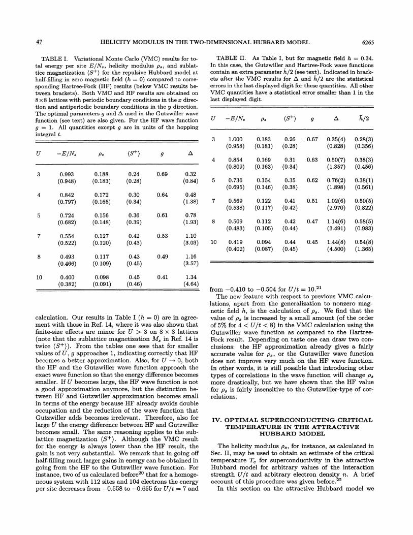
In Tables I and II, we compile results of VMC calcula-tions for both the ground-state energy per site Z/N, andthe helicity modulus p, for a set of values of the interac-tion strength U/t in zero field (Table I) and in a smallfield h/t = 0.34 (Table II). We also compare with the cor-responding results from the Hartree-Fock calculation,which for meaningful comparison have also been calcu-lated on 8 x 8 lattices and with periodic (antiperiodic)boundary conditions in the x direction (y direction). Inthe Hartree-Fock calculation, it is easy to investigate thefinite-size effect. We find that for the values of U in thetables the effect of going to larger lattices occurs in deci-mals not displayed in the tables. For U & 3 the size effectbecomes significant. We expect the finite-size efFect to beroughly the same in the VMC calculation as in the HF


TABLE I. Variational Monte Carlo (VMC) results for to-tal energy per site E/N„helicity modulus p„and sublat-tice magnetization (8+) for the repulsive Hubbard model athalf-filling in zero magnetic field (h = 0) compared to corre-sponding Hartree-Fock (HF) results (below VMC results be-tween brackets). Both VMC and HF results are obtained on8 x 8 lattices with periodic boundary conditions in the x direc-tion and antiperiodic boundary conditions in the y direction.The optimal parameters g and 4 used in the Gutzwiller wavefunction (see text) are also given. For the HF wave function

g = 1. All quantities except g are in units of the hoppingintegral t.

E/N, —

U E/N—, h/2

1.000(0.958)

0.183 0.26(0.181) (0.28)

0.67 0.35(4) 0.28(3)(0.828) (0.356)

TABLE II. As Table I, but for magnetic field h = 0.34.In this case, the Gutzwiller and Hartree-Fock wave functionscontain an extra parameter h/2 (see text). Indicated in brack-ets after the VMC results for K and h/2 are the statisticalerrors in the last displayed digit for these quantities. All otherVMC quantities have a statistical error smaller than 1 in thelast displayed digit.

0.993(0.948)

0.842(0.797)

0.188(0.183)

0.172(0.165)

0.24(0.28)

0.30(0.34)

0.69

0.64

0.32(0.84)

0.48(1.38)

0.854(0.809)

0.736(0.695)

0.569(0.538)

0.169 0.31(0.163) (0.34)

0.154 0.35(0.146) (0.38)

0.122 0.41(0.117) (0.42)

0.63 0.50(7) 0.38(3)(1.357) (0.456)

0.62 0.76(2) 0.38(1)(1.898) (0.561)

0.51 1.02(6) 0.50(5)(2.970) (0.822)

0.724(0.682)

0.554(0.522)

0.493(0.466)

0.156(0.148)

0.127(0.120)

0.117(0.109)

0.36(0.39)

0.42(0.43)

0.43(0.45)

0.61

0.53

0.49

0.78(1.93)

1.10(3.o3)

1.16(3.57)

10

0.509(0.483)

0.419(o.4o2)

0.112(0.105)

0.094(0.087)

0.42(0.44)

0.44(0.45)

0.47 1.14(6) 0.58(5)(3.491) (0.983)

0.45 1.44(8) 0.54(8)(4.500) (1.365)

10 0.400(O.382)

0.098(0.091)

0.45(o.46)

0.41 1.34(4.64)

calculation. Our results in Table I (h = 0) are in agree-ment with those in Ref. 14, where it was also shown thatfinite-size efFects are minor for U & 3 on 8 x 8 lattices(note that the sublattice magnetization M, in Ref. 14 istwice (8+)). From the tables one sees that for smallervalues of U, g approaches 1, indicating correctly that HFbecomes a better approximation. Also, for U -+ 0, boththe HF and the Gutzwiller wave function approach theexact wave function so that the energy difFerence becomessmaller. If U becomes large, the HF wave function is nota good approximation anymore, but the distinction be-tween HF and Gutzwiller approximation becomes smallin terms of the energy because HF already avoids doubleoccupation and the reduction of the wave function thatGutzwiller adds becomes irrelevant. Therefore, also forlarge U the energy difFerence between HF and Gutzwillerbecomes small. The same reasoning applies to the sub-lattice magnetization (8+). Although the VMC resultfor the energy is always lower than the HF result, thegain is not very substantial. We remark that in going ofFhalf-filling much larger gains in energy can be obtained ingoing from the HF to the Gutzwiller wave function. Forinstance, two of us calculated before that for a homoge-neous system with 112 sites and 104 electrons the energyper site decreases from —0.558 to —0.655 for U/t = 7 and

from —0.410 to —0.504 for U/t = 10.zThe new feature with respect to previous VMC calcu-

lations, apart from the generalization to nonzero mag-netic field h, is the calculation of p, . We find that thevalue of p, is increased by a small amount (of the orderof 5'Fo for 4 ( U/t ( 8) in the VMC calculation using theGutzwiller wave function as compared to the Hartree-Fock result. Depending on taste one can draw two con-clusions: the HF approximation already gives a fairlyaccurate value for p„or the Gutzwiller wave functiondoes not improve very much on the HF wave function.In other words, it is still possible that introducing othertypes of correlations in the wave function will change p,more drastically, but we have shown that the HF valuefor p, is fairly insensitive to the Gutzwiller-type of cor-relations.

IV. OPTIMAL SVPERCONDUCTING CRITICALTEMPERATURE IN. THE ATTRACTIVE

HUBBARD MODEL

The helicity modulus p„ for instance, as calculated inSec. EI, may be used to obtain an estimate of the criticaltemperature T, for superconductivity in the attractiveHubbard model for arbitrary values of the interactionstrength U/t and arbitrary electron density n Abrief.account of this procedure was given before. ~

In this section on the attractive Hubbard model we


can use the formulas derived in Sec. II for the repulsiveHubbard model if some "translations" are made. Ac-cording to the "spin-down particle-hole" transformationone must replace in (37), (40), (41), and (48) the mag-netization m by the deviation from half-filling n —1 andthe effective Zeeman field h/2 by the effective chemicalpotential p [see (19) and (20)].

For weak attraction, the Hartree-Fock approximationis a good approximation and for the Hubbard model on asquare lattice gives results that are qualitatively similarto the results of the BCS theory for superconductivity(see, e.g. , Ref. 23). For instance, for small ~U~/t thegap parameter at zero temperature 4(0) decreases expo-nentially for decreasing ~U~/t. From (40) and (41) oneobtains

0) 32ge— g/I I for n=1, (79)

a(O) = 9~e (80)

The critical temperature for superconductivity T, (HF)follows from (40) and (41) with the additional conditionE(T,) = 0. We find A(0)/k~T, = 1.80 in the small-Ulimit, whereas standard BCS theory gives 1.764 for thisratio. The temperature dependence of the gap near T, isgiven by

for n = 0.5.

(81)

where in the small-U limit n = 1.74, exactly as in theBCS theory. It is somewhat remarkable that this be-havior near T, is very robust for all values of ~U~/t: inthe limit of ~U~/t —+ oo, n is minimal: n = ~3 = 1.73,whereas o. reaches a maximum for ~U~/t 5.6 of only1.75. Also, the ratio 6(0)/k~T, never exceeds the value2, which is the limiting value for ~U~/t —+ oo.

It has been argued and illustrated by severalresearchers 47 s that the BCS (or HF) approximationto the wave function remains an appropriate form forthe wave function for all values of ~U~/t. In the large-U regime, the wave function would then describe a gasof tightly bound electron pairs which will exhibit localpair (LP) or bipolaronic superconductivity. The super-conducting transition then corresponds to the superfluidtransition of a hard-core Bose gas of such pairs (no twopairs may occupy the same site because of the Pauli ex-clusion principle). Since in the limit of strong attrac-tion the model can be mapped onto a pseudo-spin-modelwith efFective interaction constant J = 4t /~U~, T, (pro-portional to J) (Ref. 7) will decrease for increasing ~U~/t'

and can no longer correspond to T, (HF) (which increaseslinearly with ~U~/t). For larger ~U~/t, low-energy excita-tions will destroy the order for a much lower temper-ature than T,(HF), which is the temperature at whichthe now tightly bound pairs break up. The evolutionfrom Cooper-pair superconductivity for small U to LPsuperconductivity for large U is thought to be smooth.Since both in the small- and large-U limit T, vanishes,evidently there must be an optimal T, for an intermedi-ate value of ~U~/t. In this section, we present a schemefrom which for the Cooper-pair superconductor, the LPsuperconductor, and everything in between the critical

temperature can be extracted. This scheme makes use ofthe helicity modulus.

The low-energy excitations that destroy the order fora lower temperature than T,(HF) can be thought of asfluctuations of the order parameter which have been ne-glected in the HFA. Here, we consider fluctuations in thephase of the order parameter. Then we have a modelsimilar to that of XY ferromagnetism, where the com-plex gap field A~ is the equivalent of an X'Y spin. Forlow enough T, the system is in a ferromagnetically or-dered state (i.e. , constant Az), whereas for higher tem-perature in two dimensions a Kosterlitz-Thouless (KT)phase transition arises. s The KT transition correspondsto the binding/unbinding of certain spin configurationscalled vortex-antivortex pairs, which correspond in thenegative-U model to certain configurations of the L~ in-volving only phase fluctuations. Thus, in this view, thesuperconducting state of the attractive Hubbard modelis a KT phase, with corresponding algebraically decayingcorrelations. Exactly at the transiton temperature T,the following relation with the spin-stiffness or helicitymodulus holds:

(82)

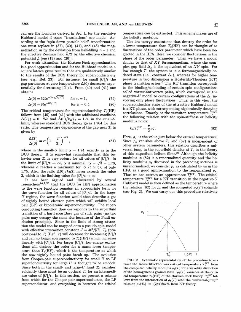
Here, p, is the value just below the critical temperature.Since p, vanishes above T, and (82) is independent ofother system parameters, this relation describes a uni-versal jump in the superfluid density at T, in the theoryof thin superfluid helium films. 2s Although the helicitymodulus in (82) is a renormalized quantity and the he-licity modulus p, discussed in the preceding sections isunrenormalized, we consider p, as calculated by us in theHFA as a good approximation to the renormalized p, .Thus we can extract an approximate T, . The criticaltemperature T, for a KT transition in the negative-UHubbard model is then defined as the temperature wherethe relation (82) for p, and the computed p, (T) coincide(see Fig. 2). We can carry out this procedure relatively

Ps

Tc Tc(HF) T

FIG. 2. Schematic representation of the procedure to ex-tract the Kosterlitz-Thouless critical temperature T, fromthe computed helicity modulus p, (T) for a wavelike distortionof the homogeneous ground state. p, (T) vanishes at the criti-cal temperature T,(HF) of the Hartree-Fock theory. T, fol-lows from the intersection of p, (T) with the "universal-jump"relation p, (T,) = (2/vr)k&T, from KT theory


easily for arbitrary combinations of the parameters ~U~/tand density n. As in the case of positive U (for which theformulas were given in Sec. II), there is a slight compli-cation in that in calculating p, (T) for fixed ~U~/t and n(which are the physical parameters), for every new T theparameters 6 and P have to be adjusted according to (40)and (41). In this way, the critical temperature for super-conductivity T, is indeed always smaller than T,(HF);the reduction is very small for small ]U~ [p, (T = 0) issizable but drops off to zero rapidly] and very large forlarge ~U~ [p, (T = 0) is small but practically constant upto the intersection point].

In Fig. 3(a), T, /t as a function of ]U~/t is shownfor three values of the filling (n = 1, n = 0.5, andn = 0.1, respectively). For small ~U~, T, is only reducedby a small amount compared to standard BCS theory,

0.4

0.3—

I

I

I

BCS '

II

II

t

I

I

I

(a)

0.2—

0.1—I

JtI

Il

II

II

000 2

I I I I

6 8 10 12 14

[U)/1

0.2

0.1

0.0 0.2 0.4 0.6 0.8 1.0

FIG. 3. Phase diagram of the 2D negative-U Hubbardmodel on a square lattice. (a) T, /t as a functioii of ~U~/t

for three difFerent fillings (n = 1, n = 0.5, and n = 0.1, respec-tively). For comparison are shown T, (HF)/t [or equivalentlyT (BCS)/t; dashed line] and the functional form mt/2~ U~ (dot-ted line) to which T /t approaches (for half-filling) for small

~U] and large ~U~, respectively. (b) T, /t as a function ofelectron density n for U/t = —2, —4, and —7.5. The quantumMonte Carlo results of Ref. 31 for U/t = —4 are denoted bytriangles (sea the discussion in Sec. V).

@B+c = 0 898JNN (83)

Again this procedure to extract T, is not rigorous, sincein our system of phase-fI. uctuating 4, the interaction isnot restricted entirely to nearest neighbors. We have ver-ified, by also computing the energy of a "Neel configura-tion" of 4, , that for ]U~/t ) 3 the next-nearest-neighborcoupling JNNN is always smaller than JNN by a factor of

whereas for very large [U~ a T, proportional to t /~U~ isindeed found, as expected because of the connection witha pseudo-spin-model with J = 4t /~U~. In Fig. 3(b), T,/tis shown as a function of n for ]U~/t equals 2, 4, and 7.5.Figure 3(b) can be extended to 1 ( n ( 2 since, be-cause of particle-hole symmetry, T,(n —1) = T, (1 —n).Therefore, within the approximations that were made,we obtain the phase diagram of the 2D negative-U Hub-bard model for the whole range of interaction strengths~U~/t and electron densities n. The maximum T, of 0.25toccurs for ~U~/t = 4 and n = 1. For large ~U~, the ratio6(0)/k~T, is of course much enhanced as compared tothe BCS (or HF) result; e.g. , in case of the optimal T,(~U~/t = 4) A(0)/k~T, = 11.1, whereas for ~U~/t = 3this ratio equals 7.3.

A deficiency of our result is that T, does not vanish athalf-filling, where one would expect that the Heisenbergsymmetry, which the system possesses at half-filling, doesnot allow for the KT phase and therefore gives T, = 0.The vanishing T, is a result of the delicate symmetrybetween charge density and pairing correlations at half-61ling. It is not surprising that we do not recover this fea-ture since our procedure cannot easily accommodate theadditional symmetry which arises at half-611ing, wherethe XY symmetry we use for all n is extended to thehigher Heisenberg symmetry. A small amount of dopingalready destroys the Heisenberg symmetry and results ina finite T~; also a small deviation from ideal two dimen-sionality results in a finite T, . Therefore our results areexpected to be good already for a small deviation fromhalf-Ailing, which in our calculation does not alter T, verymuch [see Fig. 3(b)], but we miss the logarithmic drop tozero when approaching half-filling.

Another point of concern regarding our procedure isthat we have borrowed the relation k~T, = (vr/2) p, fromthe exact, renormalized KT theory, whereas our calcu-lated p, is unrenormalized. The fact that p, is unrenor-malized will decrease the estimate for T, ; the resultswe give are upper bounds in this respect. 6'26 We haveinvestigated this effect by studying another, inhomoge-neous, excitation of the ground state with constant 4, .We compute by exact diagonalization of the Bogoliubov-deGennes equations (23) and (24) on small lattices (8x 8)the excitation energy AE of turning one A; to —4, as afunction of ~U~/t (for half-filling and T = 0). This raisein energy we relate to a nearest-neighbor interaction con-stant JNN between (ferromagnetic) A Y spins by equatingAE to 8JNN. Subsequently, we use the relation betweenthe interaction constant JNN and the critical tempera-ture T, for the phase transition in the two-dimensionalXY ferromagnet (with nearest-neighbor coupling only)as found in recent Monte Carlo calculations: 7

6268 DENTENEER, AN, AND van I.EEU%'EN

TABLE III. Critical temperature T, for a Koster-litz-Thouiess (KT) type of phase transition for a system ofphase-Buctuating gap parameters 4 as a function of U athalf-filling and zero magnetic field. If the system is taken tobe identical to a nearest-neighbor ferromagnetic XY model,i"sT, = 0.898JNN (taken from Ref. 27), with JNN the cou-pling constant. The calculation of JNN is explained in thetext. If the system is taken to obey the universal-jump rela-tion of KT theory, k&T, is obtained using a Hartree-Pockcalculation of the helicity modulus p, (T) by an intersectionprocedure (see Fig. 2). For comparison p, (T = 0) is listedin the last column; p, (T = 0) and JNN become equal in thelimit of large U. All results in the table are obtained on 8 x 8lattices and are in units of the hopping integral t. 2

lim — yRpz(q, ~) = p, q + O(q ).44J ~OO

(84)

for the doped negative-U model obtained in this paper.First, we discuss results to be compared with p, and lateron results to be compared with T, .

We have found that p,—as calculated in the HFA inSec. II for the repulsive case for half-filling and arbitraryU/t, T, and h—for the special case of T = 0 and h = 0coincides exactly (for all values of U/t) with a particu-lar long-wavelength large-frequency limit of the dynamictransverse susceptibility y+ (q, w) as calculated in therandom-phase approximation (RPA):

JNN

WAXY

p, (T = 0)

0.81.01.21.41.62.02.43.03.33.64.05.06.0

2.873.273.654.024.405.125.856.957.508.058.80

10.6812.59

0.07500.10200.13100.13760.13?40.13340.12700.11600.11060.10560.09900.08520.0742

0.0670.0920.1180.1240.1230,1200.1140.1040,0990.0950.0890,0770.067

0.2240.2440.2510.2510.2450.2300.2130.1900.1800.1700.1590.1360.118

0.1830.1770.1710.1640.1580.1460.1350.1210.1140.1080.1010.0860.075

at least about 2 (JNNN can have either sign). In TableIII, we compare T, + with TK obtained by the inter-section procedure using p, from the HFA We al. so list

p, (T = 0) as calculated in the HFA. For better compar-ison, both T, and p, (T = 0) have been calculated onsxs lattices. For the range of values of U considered thefinite-size efr'ect is negligible. From the table it is clearthat T, is smaller than T, by a factor of about 2 formost of the U values considered. Note that like T,T, + goes through a maximum, which furthermore oc-curs for about the same value of ~U~/t. However, Tx+drops off much more rapidly for decreasing ~U~/t. Wealso note that p, (T = 0) does not go through a maxi-mum; the nonmonotonous behavior of T, is due to ourintersection procedure. The fact that both critical tem-peratures show the same qualitative behavior can be seenas a sign of the consistency of our arguments. Finally,we note that in the large-U limit p, (T = 0) and JNNcoincide.

V. CONNECTION WITH PREVIOUSAPPROACHES AND DISCUSSION

Several results obtained in the literature on the two-dimensional Hubbard model can be related to results forthe helicity modulus p, and the critical temperature T,

This specific limit can be shown to be equal to the firstmoment (a) of the dynamic structure factor S~(q, w)associated with spin-spin correlations, a relation knownas the f-sum rule. 2 Equation (84) is derived in detailin Appendix B, starting from the RPA calculations aspublished before by several groups. i In Ref. 12, thelarge-U limit of the f-sum rule was found to be (~) =q2t2/U, in agreement with (84) (see Appendix B). Ourresults for p, generalize the f-sum rule for the positive-UHubbard model at half-filling to arbitrary U/t.

Our result for the optimal critical temperature for su-perconductivity in the attractive Hubbard model canalso be brought in connection with results in the lit-erature. A large number of papers has been devotedto the question of a smooth transition from a BCS-likesuperconducting-normal transition for small U to a Bose-Einstein-like superfluid-normal transition (or local-pairsuperconductor-normal transition) for large U. 7

In some of these papers even a qualitative phase diagramlike Fig. 3 is drawn. " We have given a quantita-tive scheme from which T, can be found for arbitrary~U~/t and arbitrary density. This scheme is based onthe helicity modulus, which we have calculated using twowell-defined approximations. We also compared the ap-proximated p, with more exact calculations (see above),showing that the HFA results for p, are fairly accurate.The weakness of our approach to extract T, lies in thefact that we invoke exact theories like that of Kosterlitzand Thouless or results from accurate Monte Carlo cal-culations on the ferromagnetic XY model which are notexactly applicable to our model. For instance, the "uni-versal jump" relation (82) from KT theory holds exactlyonly for the case that the core energy E, associated witha vortex is infinitely large. If not, T, will be lower. Forinstance, the ferromagnetic XY model on a square latticehas a finite E,. It would be interesting to see what wouldbe the core energy for vortices in a system of gap param-eters which are phase fIuctuating over the lattice. Thatindeed the actual T, for the Hubbard model can be muchlower than extracted from p, HFA we already sho~ed inSec. IV, by finding T, from an effective nearest-neighborcoupling constant for a ferromagnetic XY model. There-fore, although we cannot claim any degree of exactness of


our result for T„we speculate that the HFA results forp, lead to an approximation for T, , which will not haveto be adjusted downward by a factor of more than about3 (for densities 1n —11 ) 0.1 and arbitrary U). Further-more, our approximation to T, can be evaluated readilyfor the whole parameter space (U/t, n). In view of theabove, the rather large difference between our result forT, and that of quantum Monte Carlo (QMC) calculations[Ref. 31 and Fig. 3(b)] is not distressing. Furthermore,although QMC calculations are arbitrarily accurate inprinciple, T, does not follow from them directly; T, wasextracted from the behavior of pairing correlations fittedto expected Kosterlitz-Thouless behavior. However, it isnot obvious that the correlation function will follow KTbehavior on the small lattices of maximally 8 x 8 thatwere used and therefore the exact T, may differ from theQMC result. An additional drawback of QMC calcula-tions is that it is very time consuming to compute T, formore than a few points in the parameter space (U/t, n).

For completeness we note that recently an optimal T,for superconductivity was found in the Gorkov model offermions with an attractive short-range interaction in twodimensions. This model can be seen as an analog of theHubbard model for the case that the fermions are not re-stricted to a lattice. The optimal T, is obtained using aprocedure similar to ours; first a Ginzburg-Landau theoryis constructed describing the crossover from BCS super-conductivity to Bose superfluidity and then the MonteCarlo result of Ref. 27 for the nearest-neighbor 2D XYmodel [see (83)] is used to extract T, . An important dif-ference with our approach is that in Ref. 32 the superfluiddensity p, is identified directly with the interaction con-stant JNN in the XY model. As can be seen from TableIII, we find this identification to be correct only for largevalues of 1U1/t.

In conclusion, we have presented detailed calculationsusing a variety of approximations of the helicity modulusin both repulsive (at half-filling) and attractive (in mag-netic field zero) Hubbard models. We furthermore usethe helicity modulus to extract a critical temperaturefor superconductivity in the attractive Hubbard modelfor arbitrary density and arbitrary interaction strengthwhich correctly interpolates between weak- and strong-coupling limits. Using the Hartree-Fock approximationfor p„which we have shown to coincide with the re-sult in the random-phase approximation for p„and theuniversal-jump relation from Kosterlitz-Thouless theory,an optimal T, of 0.25t is found for U/t = —4. We havegiven estimates of the deviation of this result from the(unknown) exact result. Finally, we have extensivelycompared our results for p, and T, with results in theliterature on the Hubbard model.

Note added. After completion of our work a paper byScalapino, White, and Zhang appeared33 which expressesthe belief that the Drude weight equals the superfluidweight in the superconducting state (see also Ref. 28). Ifthis belief is borne out, the possibility is opened of com-paring our calculations for p, with the extensive exactdiagonalization calculations of the Drude weight in thenegative-U Hubbard model of Ref. 34. This possibility ispresently being investigated by us.

ACKNOWLEDGMENTS

We acknowledge illuminating discussions with D.A.Huse on the variational Monte Carlo calculation of thehelicity modulus. We further acknowledge financial sup-port from the Foundation for Fundamental Research onMatter (FOM) (G.A.).

APPENDIX A

(A3)

where P = 1/k~T and Z is the partition function:

Z = Tr(e i'~). (A4)

The minimum value E[p] attains is exactly the free en-

ergy:F = —kggTlnZ. A

Now we consider the Hartree-Fock approximation tothe Hubbard Hamiltonian (1) which allows for antiferro-magnetic ordering, i.e. , allowing for nonvanishing aver-ages (S, ) besides nonzero averages (n, ). The approx-imated Hamiltonian is given by [as in Sec. II; see (13),but now with temperature-dependent fields]

with the Hermitian matrix H,~ j given by

herH, ~

= t ~+1 U(n, —)p— )—U(S, )pbi~b (A7)

At this point the fields (S, )p and (n, )p are just pa-

We show that at finite temperatures the Hartree-Fockapproximation (HFA) can be formulated as a variationalsearch for self-consistent fields (n, )p and (S, )p, wherethe subscript denotes the temperature dependence of thefields. For finite temperatures, the quantity to be mim-imized turns out to be the Hartree-Fock (HF) free energyFiick (to be defined below); moreover optimal fields (A) pturn out to be given by HF averages:

(A) p = Tr(piipA).

In (Al), pili; is the density matrix associated with theHartree-Fock approximation to the Hamiltonian (to bedefined below). This variational principle thus general-izes the T = 0 HFA of Sec. II A to finite temperatures.

Consider the functional X[p]:

P[p] = Tr(p'8 + kriTpln p), (A2)

working on the space of normalized N-body density oper-ators p (Trp = 1). Using the normalization of the densityoperator, it follows that P[p] is minimized by the Boltz-mann operator


rameters, which will be identified with averages below.The one-electron HF energies e(k) follow from the HFequations [cf. (8)]:

).~'-, ~ &~- (k) =~(k)4'-(k) (A8)

&[PHF] = +HF~ (A9)

which is a special property of the HFA and not true foran arbitrary approximation to the Hamiltonian. Using(A6) and evaluating the trace in the basis of the 2N,eigenstates of H,~~ (N, is the number of sites of thelattice), the HF free energy is

FHF = ——) ln I+e-i'~"l

—U).(( ' ) ( ') —(S,+) (S, ) ) (A10)

Considering the fields (S, )p and (n, )p as four inde-pendent parameters one straightforwardly finds the fieldsthat optimize FHF. As an example we take (n, t )p. From(A10) one finds

We now proceed to show that the fields (S, )p and(n, ) p that optimize the HF free energy FHF [defined by(A5) using 'MHF in (A4) to obtain ZHF] also optimizeE[p]. In other words, we show

explicit dependence of H, ~ on (n;y) p needs to be takeninto account:

Be(k) ) - . („)BHi, , („)B(~.T)i,...,' B(~.t)p "

= U14"i(k) I'. (A13)

Applying similar considerations to the other fields, onearrives at the following consistency equations for thefields:

(&* )p = ).I&* (k) I'&(k)

(S, )p =) P; (k)P, (k)n(k).

(A14)

(A15)

(n,~)HF = Tr(pHFii, ~) = (ri,~)p

(s, )HF:—T (pHFS, ) = (S, )~.(A16)(A17)

Using the definition of the free-energy functional E[p](A2), one finds that

+[pHF] Tr [pHF(+ +HF)] + +HF. (A18)

Note that Eqs. (A14) and (A15) are straightforwardfinite-temperature generalizations of Eqs. (9) and (10).Working again in the basis of eigenstates of H, ~, oneeasily verifies that the finite-temperature Hartree-Fockaverages of n; and S, are given precisely by the fieldsin (A14) and (A15):

where n(k) is the Fermi-Dirac distribution:

(A11) The difference between the original and HF Hamiltonianis found just in the on-site interaction term. Evaluatingthe HF average of this difference, while invoking Wick'stheorem to show that

- —1n(k) = I+.P ~"l (A12) (&']'&'t. )HF (&'1')HF(%J)HF (S' )HF(S' )HF (A19)

For the derivative of e(k) we use (A8), in which only the one obtains for arbitrary (S, )p and (n, )p

(+ +HF)HF = U) [((&'t')HF (ii'T)P)((&'J)HF (&'J)P) ((S )HF (S )P)((S' )HF (S )P)] ~ (A20)

Obviously the optimal fields, which obey (A16) and(A17), make the HF average of the difference zero, but,furthermore, adding (A20) to FHF will not change theoptimization equations (A14) and (A15) since the addedterm is quadratic in the deviations. Therefore, the opti-mized fields of the HFA optimize FHF and P[pHF] at thesame time.

APPENDIX B

random-phase approximation (RPA). More specifically,we show

(dlim — y+ (q, ~) = p, q +O(q ). (B1)

The RPA was applied to the positive-U Hubbard modelat half-filling in zero magnetic field by several groups.Here we follow Ref. 12, in which the following expres-sion for the dynamic transverse susceptibility is given (weomit the so-called umklapp branch, since we will be in-terested in the small-q limit):

We show that the helicity modulus as obtained in theHartree-Fock approximation in Sec. II, Eq. (48), is iden-tical to a small-wave-vector, large-frequency limit of thedynamic transverse susceptibility as calculated in the

gll —U(gllX22 —+12+21)x+ (q, ~) =(1 —UXil) (1 —UX22) —(UXi2) 2'

where

(B2)


xii(q~~) = 2~). I1 —

E I (f +f+)1

P2N - ( E+

parameter A. This is not obvious from the sum on firstinspection; however, one may use the identity

Xi2(q, ~) =2~).' E E (f —-f+)p

xzi(q, ~) = xi2(q, ~)x22(q, ~) =xii(Q —q, ~)

(B5)(B6)

(& —2e2~) sin p e cosyE5 2E3 (B15)

[+(p)] =—~ ) +(&) (B16)

where we have taken t = 1 and introduced the notation

fy =—(E++ E +~)E~ —— ez~+ ~a]',

p+q/2~

ep = —2t(cos pz + cos py).

(B8)

(B9)(B10)

Note that e~ is the g = 0 expression for e~. Analogously,the q = 0 expression for E~ is denoted by Ep:

The prime on the summation indicates the restriction tothe magnetic Brillouin zone (MBZ): pz +p„e [

—vr, vr] andQ = (a, vr) Th.e following abbreviations are introduced:

The identity (B15) may be proved by noting that thesummand is a derivative with respect to pz of a functionthat is periodic in p . Using (B12) and (B13),we obtainthe desired limit as

(dlim — X+ (q, to) =26 yq +O(q ). (B17)

We now proceed to show that the prefactor of the q2

term in (B17), 26zy, is exactly p, as calculated in theHFA, formula (48), for T = 0 and h = 0. Using thenotation introduced above, for this case p, is given by

Ep —— ez + ~K~2. (Bll) p, (T =O, h=0) = (B18)

First, we consider the large-u limit. The only frequencydependence is in the functions fy. Because for large fre-quencies Xii and X2z are proportional to w and Xiz isproportional to cu, we can neglect the product yqqy22in the numerator. Second, the leading term of the denom-inator in the large-u, small-q limit is just 1. Therefore,we require only the limiting behavior of xii and xi'. Af-ter a straightforward, but tedious, calculation one findsto leading order for large cu and small q

Note that in (48) a sum over the full Brillouin zone ap-pears, whereas here we have a sum over the MBZ. Forsummands which are (i) invariant under interchange ofpz and py and (ii) invariant under a simultaneous changeof sign of all sines and cosines the sum over the full BZis twice the sum over the MBZ. To derive (B18) we havemade use of this property. Finally, to prove (Bl) we usean identity similar to (B15),which is proved analogously.With the identity

462 (1Xii= z I U+W2

+12 —+21 ~U'

sin pz e~ cos pzE3 2Ep

(B13) it follows easily that

(B19)

where y is given by the following sum over the MBZ: p, (T = 0, h = 0) = 2b, zy, (B20)2 ~ 2

&scn p~E3

p p(B14)

We remark that the q /u term in Xi2 is proportional toa sum over the MBZ which vanishes for all values of the

which together with (B17) proves (Bl). Our result in-cludes the large-U limit discussed in Ref. 12: (to)(J/4)q2, where J = 4t2/U is the effective interactionconstant for large U. In that limit, one finds from theabove that p, = 262y = t /U = J/4.

*Present address: Shell Research BV, P.O. Box 60, 2280 ABRijswijk, The Netherlands.

~M.C. Gutzwiller, Phys. Rev. Lett. 10, 159 (1963); J. Hub-bard, Proc. R. Soc. (London) Ser. A 276, 238 (1963); J.Kanamori, Prog. Theor. Phys. (Kyoto) 30, 275 (1963);P.W. Anderson, Phys. Rev. 115, 2 (1959).P.W. Anderson, Science 235, 1196 (1987).M.E. Fisher, M.N. Barber, and D. Jasnow, Phys. Rev. A 8,1111 (1973).

4R.R.P. Singh and D.A. Huse, Phys. Rev. B 40, 7247 (1989).sE. Manousakis, Rev. Mod. Phys. 63, 1 (1991).

J.M. Kosterlitz and D.J. Thouless, J. Phys. C 6, 1181(1973).R. Micnas, J. Ranninger, and S. Robaszkiewicz, Rev. Mod.Phys. 62, 113 (1990).J.A. Verges, E. Louis, P.S. Lomdahl, F. Guinea, and A.R.Bishop, Phys. Rev. B 43, 6099 (1991).

9P.G. deGennea, Superconductivity of Metals and Alloys(Benjamin, New York, 1966).We have taken q to be (q, 0) with q g [O,z] but this is notessential.J.R. SchriefI'er, X.G. Wen, and S.C. Zhang, Phys. Rev. B


89, 11663 (1989); A. Singh and Z. Tesanovic, ibid 4.1, 614(1990).H. Monien and K.S. Bedell, Phys. Rev. B 45, 3164 (1992).M.C. Gutzwiller, Phys. Rev. 187, A1726 (1965).H. Yokoyama and H. Shiba, J. Phys. Soc. Jpn. 56, 3582(1987).T. Giamarchi and C. Lhuillier, Phys. Rev. B 42, 10641(1990).D. Ceperley, G.V. Chester, and M.H. Kalos, Phys. Rev. B16, 3081 (1977).C.J. Umrigar, K.G. Wilson, and J.%'. Wilkins, Phys. Rev.Lett. 60, 1719 (1988).W. Kohn, Phys. Rev. 138, A171 (1964).Since in the VMC calculation, the average of 'H is calculatedwithout the chemical potential term, whereas the ground-state energy in the HFA is calculated including the chemicalpotential, to the energy given in (25) a constant pN, has tobe added to obtain the ground-state energy at a fixed num-ber of particles. At half-filling, this constant equals N, U/2.In this way, the ground-state energy at half-filling goes tozero in the limit of infinitely large U.Guozhong An and J.M.J. van Leeuwen, Phys. Rev. B 44,9410 (1991).Table III in Ref. 20 contains a printing error: the ground-state energy using the Gutzwiller wave function (EGwF) forthe commensurate phase (GWF CM) for U/t = 10 shouldbe —56.46 instead of —54.46.

~ P.J.H. Qenteneer, Guozhong An, and J.M, J. van Leeuwen,

Europhys. Lett. 16, 5 (1991);16, 509(E) (1991).sM. Tinkham, Introduction to Superconductivity (McGraw-

Hill, Kogakusha, 1975).P. Nozieres and S. Schmitt-Rink, J. Low-Temp. Phys. 59,195 (1985); A.J. Legget, Modern Trends in the Theory ofCondensed Matter (Springer, Berlin, 1980), p. 13.M. Randeria, J.-M. Duan, and L.-Y. Shieh, Phys. Rev. B41, 327 (1990).D.R. Nelson, in Fundamental Problems in Statistical Me-chanics V, edited by E.G.D. Cohen (North-Holland, Am-sterdam, 1980).R. Gupta, J. DeLapp, G.G. Batrouni, G.C. Fox, C.F. Bail-lie, and J. Apostolakis, Phys. Rev. Lett. 61, 1996 (1988).B.S. Shastry and B. Sutherland, Phys. Rev. Lett. 65, 243(1990).R.T. Scalettar, E.Y. Loh, J.E. Gubernatis, A. Moreo, S.R.White, D.J. Scalapino, R.L. Sugar, and E. Dagotto, Phys.Rev. Lett. 62, 1407 (1989).D.I. Khomskii and A.K. Zvezdin, Solid State Commun. 66,651 (1988).A. Moreo and D.J. Scalapino, Phys. Rev. Lett. 66, 946(1991).M. Drechsler and W. Zwerger (unpublished).D.J. Scalapino, S.R. White, and S.C. Zhang, Phys. Rev.Lett. 68, 2830 (1992).D.J.Scalapino, Physica C 185-189,104 (1991);E. Dagotto,A. Moreo, F. Ortolani, J. Riera, and D.J. Scalapino, Phys.Rev. B 45, 10107 (1992).

Date post:	13-Mar-2020
Category:	Documents
Upload:	others
View:	3 times
Download:	0 times

Helicity modulus in the two-dimensional Hubbard modeljmjvanl/helicity.pdf · Helicity modulus in...

Documents