Set up Security Permissions on Remote Machine . . . . . . . . . . . . . . . . . 13-7Solve a Test Design as a Remote User on a Remote Machine . . . . . . . . . 13-7
Setting the Maximum Iterations for an Optimization Analysis . . . . . . . 14-10Adding a Cost Function . . . . . . . . . . . . . . . . . . . . . . . . . . . . . . . . . . . . . 14-10
Specifying a Solution Quantity for a Cost Function Goal . . . . . . . . . . . . . 14-11Setting the Calculation Range of a Cost Function Goal . . . . . . . . . . . . . . . 14-12Setting a Goal Value . . . . . . . . . . . . . . . . . . . . . . . . . . . . . . . . . . . . . . . . . 14-12
Specifying a Single Goal Value . . . . . . . . . . . . . . . . . . . . . . . . . . . . . 14-13Specifying an Expression as a Goal Value . . . . . . . . . . . . . . . . . . . . . 14-13Specifying a Variable-Dependent Goal Value . . . . . . . . . . . . . . . . . . 14-13
Overriding the Min. and Max. Variable Values for a Single Optimization Setup 14-15Changing the Min. and Max. Variable Values for Every Optimization Setup 14-15
Setting the Min. and Max. Step Sizes . . . . . . . . . . . . . . . . . . . . . . . . . . 14-15Setting the Min and Max Focus . . . . . . . . . . . . . . . . . . . . . . . . . . . . . . . 14-16Solving a Parametric Setup Before an Optimization . . . . . . . . . . . . . . . 14-17Solving a Parametric Setup During an Optimization . . . . . . . . . . . . . . . 14-17Automatically Updating a Variable’s Value After Optimization . . . . . 14-17
Specifying a Solution Quantity for an Output Parameter . . . . . . . . . . . . . 14-20Setting the Calculation Range of an Output Parameter . . . . . . . . . . . . . . . 14-21Overriding the Min. and Max. Variable Values for a Single Sensitivity Setup 14-22Changing the Min. and Max. Variable Values for Every Sensitivity Setup 14-22
Overriding the Distribution Criteria for a Single Statistical Setup . . . . . . 14-26Changing the Distribution Criteria for Every Statistical Setup . . . . . . . . . 14-27
HFSS is an interactive software package for calculating the electromagnetic behavior of a structure. The software includes post-processing commands for analyzing this behavior in detail. Using HFSS, you can compute:• Basic electromagnetic field quantities and, for open boundary problems, radiated near and far
fields.• Characteristic port impedances and propagation constants.• Generalized S-parameters and S-parameters renormalized to specific port impedances.• The eigenmodes, or resonances, of a structure.You are expected to draw the structure, specify material characteristics for each object, and identify ports and special surface characteristics. HFSS then generates the necessary field solutions and associated port characteristics and S-parameters.
As you set up the problem, HFSS allows you to specify whether to solve the problem at one spe-cific frequency or at several frequencies within a range.
Note If you are using the Eigenmode Solution solver, you do not need to specify sources for the problem. HFSS calculates the resonances for the model based on the geometry, materials, and boundaries.
Getting Started with HFSS 1-1
HFSS Online Help
System RequirementsHFSS supports the following operating systems:
• Windows• Sun Solaris• HP-UX• Red Hat Enterprise Linux v3
On all systems when you run HFSS for the first time (that is, with no project directory specified in the registry), or if the project directory or the temp directory does not exist, HFSS displays a dialog that asks you to set the project and temp directories. For the temp directory, there is a comment ask-ing you to ensure that adequate disk space is available.
HFSS 10 requires at least FLEXlm for Ansoft v10.1 license server.
WindowsSupported Platforms
• Windows 2000 Professional• Windows XP Professional• Windows XP Professional x64 Edition• Windows Server 2003
32-Bit System RequirementsMinimum System Requirements
Processor: All fully compatible 686 (or later) instruction set processors, 500 MHzHard Drive Space (for HFSS software): 200 MBRAM: 512 MB
Recommended Minimum ConfigurationProcessor: All fully compatible 786 (or later) instruction set processors, 1 GHzHard Drive Space (for HFSS software and temporary files): 500 MBRAM: 2 GB
Increasing RAM on 32-Bit PCUsers with the appropriate Windows OS can take advantage of potentially all the installed RAM up to a limit of 3 GB on 32-bit PCs. Doing so also requires setting up the appropriate OS
Note If you attempt to run HFSS and get a message reporting a corrupted license file, please contact Ansoft.
1-2 Getting Started with HFSS
HFSS Online Help
boot.ini switch (/3GB) to tell the OS that 3 GB is to be used for application space and only one GB for the OS kernel and related overhead.
64-bit System RequirementsMinimum System Requirements:Supported processors: AMD Athlon 64, AMD Opteron, Intel Xeon with Intel EM64T support, Intel Pentium 4 with Intel EM64T support Hard Drive Space (for HFSS software): 200 MBRAM: 2 MBRecommended Minimum Configuration (for Optimal Performance) Supported processors: AMD Athlon 64, AMD Opteron, Intel Xeon with Intel EM64T support, Intel Pentium 4 with Intel EM64T support Video card: 128-bit SVGA or PCI Express video card Hard Drive Space (for HFSS software and temporary files): 700 MBRAM: 8 GB
Note If you are using the NVIDIA Quadro2 MXR/EX video card on Windows 2000 or Windows XP, you should also download Version 40.41 or greater video driver, available for download at http://www.nvidia.com..
Minimum System RequirementsProcessor: UltraSparc v9 processor, 450 MHzHard Drive Space (for HFSS software): 550 MBRAM: 1 GB
Recommended Minimum ConfigurationProcessor: UltraSparc v9 dual processor or better, 900 MHzHard Drive Space (for HFSS software and temporary files): 800 MBRAM: 4 GB
Note You must install Sun OpenGL libraries before installing and running HFSS. This is available for free download at:http://wwws.sun.com/software/graphics/opengl/download.html .
Note Some older graphics cards may have minor display issues (such as the appearance of check marks or “t” in a report title. .
Minimum System RequirementsProcessor: PA-RISC 2.0 processor, 450 MHzHard Drive Space (for HFSS software): 750 MBRAM: 1 GB
Recommended Minimum ConfigurationProcessor: PA-RISC 2.0 dual processor or better, 900 MHzHard Drive Space (for HFSS software and temporary files): 1.5 GBRAM: 4 GB
Red Hat Enterprise Linux v3If you attempt to open an HFSS v9 project in Linux, you receive an error message that the project must first be converted to HFSS v10. This must be done using the -BatchSave command on a non-Linux system running HFSS v10. See the discussion here.
32-bit System RequirementsMinimum System Requirements:Processor: All fully compatible 686 (or later) instruction set processors, 500 MHz Hard Drive Space (for HFSS software): 200 MBRAM: 512 MBRecommended Minimum Configuration (for Optimal Performance):Processor: All fully compatible 786 (or later) instruction set processors, 2 GHz Hard Drive Space (for HFSS software and temporary files): 700 MBRAM: 4 GB
64-bit System RequirementsMinimum System Requirements:Supported processors: AMD Athlon 64, AMD Opteron, Intel Xeon with Intel EM64T support, Intel Pentium 4 with Intel EM64T support Hard Drive Space (for HFSS software): 200 MBRAM: 2 MBRecommended Minimum Configuration (for Optimal Performance): Supported processors: AMD Athlon 64, AMD Opteron, Intel Xeon with Intel EM64T support, Intel Pentium 4 with Intel EM64T support Video card: 128-bit SVGA or PCI Express video card Hard Drive Space (for HFSS software and temporary files): 700 MBRAM: 8 GB
Getting Started with HFSS 1-5
HFSS Online Help
The HFSS DesktopThe HFSS desktop consists of several windows, a menu bar, toolbars, and a status bar. Click a link below to view more information about that desktop component.
Working with the Menu BarThe menu bar enables you to perform all HFSS tasks, such as managing project files, customizing the desktop, drawing objects, and setting and modifying all project parameters. To open a help topic about an HFSS menu command, press Shift+F1, and then click the command or toolbar icon.
Project Manager
Menu barToolbars
Message Manager
Property window
Progress window
3D Modeler window
Status bar
1-6 Getting Started with HFSS
HFSS Online Help
HFSS contains the following menus, which appear at the top of the desktop:
Related TopicsGetting Help
File menu Use the File menu commands to manage HFSS project files and printing options.
Edit menu Use the Edit menu commands to modify the objects in the active model and undo and redo actions.
View menu Use the View menu commands to display or hide desktop components and model objects, modify 3D Modeler window visual settings, and modify the model view.
Project menu Use the Project menu commands to add an HFSS design to the active project, view, define datasets, and define project variables.
Draw menu Use the Draw menu commands to draw one-, two-, or three-dimensional objects, and sweep one- and two-dimensional objects.
3D Modeler menu Use the 3D Modeler menu commands to import, export, and copy Ansoft 2D Modeler files and 3D Modeler files; assign materials to objects; manage the 3D Modeler window’s grid settings; define a list of objects or faces of objects; control surface settings; perform boolean operations on objects; and set the units for the active design.
HFSS menu Use the HFSS menu to setup and manage all the parameters for the active project. Most of these project properties also appear in the project tree.
Tools menu Use the Tools menu to modify the active project’s material library, arrange the material libraries, run and record scripts, update project definitions from libraries, customize the desktop’s toolbars, and modify many of the software’s default settings.
Window menu Use the Window menu commands to rearrange the 3D Modeler windows and toolbar icons.
Help menu Use the Help menu commands to access the online help system and view the current HFSS version information.
Getting Started with HFSS 1-7
HFSS Online Help
Working with the ToolbarsThe toolbar buttons and shortcut pull-down lists act as shortcuts for executing various commands.To execute a command, click a toolbar button or click a selection on the shortcut pull-down list. To open a help topic about a toolbar button’s functionality, press Shift+F1, and then click the tool-bar button or a command in the shortcut pull-down list.To display a brief description of the toolbar button, move the pointer over the button or shortcut pull-down list.
Working with the Shortcut MenusA variety of shortcut menus — menus that appear when you right-click a selection — are available in the toolbars area of the desktop, in the 3D Modeler window, and in the Project Manager window.
Shortcut Menu in the Toolbars AreaUse the shortcut menu in the toolbars area of the desktop to show or hide windows or toolbars, and customize the toolbars.To access the shortcut menu in the toolbars area:
Hint To modify the toolbars on the desktop, do one of the following:• On the Tools menu, click Customize. • Right-click the history tree, and then click Customize on the shortcut menu. To reset to toolbars to the default positions and settings:• On the Tools menu, click Customize. On the Customize dialog box, click Reset
All.
Shortcut menu in the toolbars area
Use the shortcut menu in the toolbars area of the desktop to show or hide windows or toolbars, and customize the toolbars.
Shortcut menu in the 3D Modeler window
Use the shortcut menu in the 3D Modeler window to select, magnify, and move options (zoom, rotate, etc.), change the view, perform boolean operations, assign materials, boundaries, excitations, or mesh operations to objects, and work with field overlays.
Shortcut menus in the Project Manager window
Use the shortcut menus in the Project Manager window to manage HFSS project and design files and design properties; assign and edit boundaries, excitations, and mesh operations; add, analyze, and manage solution setups; add optimetrics analyses; create post-processing reports; insert far- and near-field radiation setups; edit project definitions; and, run Ansoft’s Maxwell SPICE.
Note All of the commands on the shortcut menus are also available on the menu bar.
1-8 Getting Started with HFSS
HFSS Online Help
• Right-click in the toolbars area at the top of the desktop.
A check box will appear next to a command if the item is visible. For example, if a check box appears next to the Project Manager command, then the Project Manager window is currently visible on the desktop. Click Customize to open the Customize dialog box, which enables you to modify the toolbar set-tings on the desktop.
Shortcut Menu in the 3D Modeler Window Use the shortcut menu in the 3D Modeler window to select, magnify, and move options (zoom, rotate, etc.), change the view, perform boolean operations, assign materials, boundaries, excita-tions, or mesh operations to objects, and work with field overlays.To access the shortcut menu in the 3D Modeler window:
Getting Started with HFSS 1-9
HFSS Online Help
• Right-click in the 3D Modeler window (grid area).
Shortcut Menus in the Project Manager WindowEach node, or item, in the project tree has a shortcut menu. For example, from the shortcut menu for the Boundaries icon, you can assign boundaries to selected objects; review information for all the boundary assignments for the active design; remove all boundary assignments; show or hide a boundary’s geometry, name, or vectors; change the priority of a previously assigned boundary; and use the PML Setup wizard to create a perfectly matched layer (PML) boundary.
1-10 Getting Started with HFSS
Working with the Status BarThe status bar is located at the bottom of the application window. It displays information about the command currently being performed.
To display or hide the status bar:• On the View menu, click Status Bar.A check box appears next to this command if the status bar is visible.Depending on the command being performed, the status bar can display the following:• X, Y, and Z coordinate boxes.• A pull-down list to enter a point’s absolute, relative, cartesian, cylindrical, or spherical coodi-
nates. • The model’s units of measurement.
Working with the Project ManagerThe Project Manager window displays the open project’s structure, which is referred to as the project tree.
The Project Manager window displays details about all open HFSS projects. Each project ulti-mately includes a geometric model, its boundary conditions and material assignments, and field solution and post-processing information.To show or hide the Project Manager window, do one of the following:• On the View menu, click Project Manager.
A check box appears next to this command if the Project Manager window is visible.• Right-click in the toolbars area on the desktop, and then click Project Manager on the short-
-11
cut menu. A check box appears next to this command if the Project Manager window is visible.
Related TopicsWorking with the Project TreeShortcut Menus in the Project Manager Window
Working with the Project TreeThe project tree is located in the Project Manager window and contains details about all open HFSS projects, as shown below:
The top node listed in the project tree is the project name. It is named Projectn by default, where n is the order in which the project was added to the current session of HFSS. Expand the project icon to view all the project’s HFSS design information and material definitions. Related TopicsViewing HFSS Design Details
Setting the Project Tree to Expand AutomaticallyYou can set the project tree to automatically expand when an item is added to a project. 1. On the Tools menu, point to Options, and then click General Options.
The Options dialog box appears. 2. Under the Project Options tab, select Expand Project Tree on Insert.
Viewing HFSS Design Details Once you insert an HFSS design into a project, it is listed as the second node in the project tree. It is named HFSSModeln by default, where n is the order in which the design was added to the project. Expand the design icon in the project tree to view all of the specific data about the model, including
-12
its boundary conditions and material assignments, and field solution and post-processing informa-tion. The HFSSModeln node contains the following project details:
Viewing the Design ListYou can use the HFSS>Design List command or the Design List icon to view a dialog with tables of the design properties. The Design list is a dialog that with tabs to let you view the following
Boundaries Displays the boundary conditions assigned to an HFSS design, which specify the field behavior at the edges of the problem region and object interfaces.
Excitations Displays the excitations assigned to an HFSS design, which are used to specify the sources of electromagnetic fields and charges, currents, or voltages on objects or surfaces in the design.
Mesh Operations Displays the mesh operations specified for objects or object faces. Mesh operations are optional mesh refinement settings that are specified before a mesh is generated.
Analysis Displays the solution setups for an HFSS design. A solution setup specifies how HFSS will compute the solution.
Optimetrics Displays any Optimetrics setups added to an HFSS design.
Results Displays any post-processing reports generated.
Port Field Display Displays all port fields in the active model.
Field Overlays Displays field overlay plots, which are representations of basic or derived field quantities on surfaces or objects. Plot folders are listed under Field Overlays. These folders store the project’s plots and can be customized. See Setting Field Plot Defaults for information on how to customize the plot folders.
Radiation Displays far- and near-field setups added to an HFSS design.
Note To edit a project’s design details:• In the project tree, double-click the design setup icon that you want to edit. A dialog box appears with that setup’s parameters, which you can then edit.
-13
Viewing Material DefinitionsThe definitions node is listed at the bottom of the project tree and displays all of the material defini-tions that are assigned to the objects in the active model.
Related TopicsAdding New Materials
Working with the Properties WindowThe Properties window displays the attributes, or properties, of an item selected in the project tree, the history tree, or the 3D Modeler window. The Properties window enables you to edit an item’s properties. The properties, and the ability to edit them in the Properties window, will vary, depend-
Model Displays the objects that comprise the model and their properties.
Boundaries Displays the boundary conditions assigned to an HFSS design, which specify the field behavior at the edges of the problem region and object interfaces.
Excitations Displays the excitations assigned to an HFSS design, which are used to specify the sources of electromagnetic fields and charges, currents, or voltages on objects or surfaces in the design.
Mesh Operations Displays the mesh operations specified for objects or object faces. Mesh operations are optional mesh refinement settings that are specified before a mesh is generated.
Analysis Setup Displays the solution setups for an HFSS design. A solution setup specifies how HFSS will compute the solution.
-14
ing on the type of item selected. The tabs available in the Properties window will also vary, depending the selection.
Related TopicsShowing and Hiding the Properties WindowSetting the Properties Window to Open Automatically
Showing and Hiding the Properties WindowTo show or hide the Properties window on the desktop, do one of the following:• On the View menu, click Property Window.
A check box appears next to this command if the Properties window is visible.• Right-click in the toolbars area at the top of the desktop, and then click Properties on the
shortcut menu. A check box appears next to this command if the Properties window is visible.
Setting the Properties Window to Open AutomaticallyTo set the Properties window to open after an object is drawn, enabling you to modify the object’s properties, do the following:1. On the Tools menu, point to Options, and then click 3D Modeler Options.
The 3D Modeler Options window appears.2. Click the Drawing tab.3. Select Edit property of new primitives.
Hereafter, after you draw an object, the Properties window will open.
-15
Modifying Object Attributes Using the Properties Window1. Select the object for which you want to edit its attributes by clicking it in the view window or
clicking its name in the history tree. 2. Under the Attribute tab in the Properties window, edit the object attribute.
Depending on the attribute type, you can edit it by doing one of the following: • Select the check box to apply the attribute; clear the check box to disable the attribute.• Click in the field and edit the numeric values or text, and then press ENTER. • Click the button and then edit the current settings in the window or dialog box that
appears. • Click the attribute, and then select a new setting from the menu that appears.
Modifying Object Command Properties Using the Properties WindowThe Command tab in the Properties window displays information about an action selected in the history tree that was performed either to create an object, such as the Draw>Box) command, or to modify an object, such as the Edit>Duplicate>Mirror command. Not all command properties can be modified. In general, the command properties that you can typ-ically modify are the numeric values, such as position values (base position, normal position, start position, etc.), size values (height, radius, etc.), and various other coordinate values. You can also modify many of the unit settings for a command property. 1. In the history tree, select the command for which you want to edit its properties.
2. Under the Command tab in the Properties window, edit the command’s properties.Depending on the property type, you can edit it by doing one of the following:• Select the check box to apply the property; clear the check box to disable the property.• Click in the field and edit the numeric values or text, and then press ENTER. • Click the button and then edit the current settings in the window or dialog box that
appears. • Click the attribute, and then select a new setting from the menu that appears.
Working with the Progress WindowThe Progress window monitors a simulation while it is running.
Hint Press and hold CTRL to select multiple commands. If you select multiple commands, only the common, or shared, properties will be displayed under the Command tab.
-16
In the image below, the Progress window is displaying the progress of a discrete frequency sweep, which is nearing completion:
To display or hide the Progress window, do one of the following:• On the View menu, click Progress Window.
A check box appears next to this command if the Progress window is visible.• Right-click the history tree, and then click Progress on the shortcut menu.
A check box appears next to this command if the Progress window is visible.
Working with the Message ManagerThe Message Manager displays messages associated with a project’s development, such as error messages about the design’s setup or informational messages about the progress of an analysis.To display or hide the Message Manager:• On the View menu, click Message Manager.A check box appears next to this command if the Message Manager is visible.
Working with the 3D Modeler WindowThe 3D Modeler window is the area where you create the model geometry. It appears to the right of the Project Manager window after you insert an HFSS design to a project.
-17
The 3D Modeler window consists of the model view area, or grid, and the history tree, as shown below:
To open a new 3D Modeler window, do one of the following:• Insert a new HFSS design into the current project.• Double-click an HFSS design in the project tree.The model you draw is saved with the current project when you click File>Save.Objects are drawn in the 3D Modeler window. You can create 3D objects by using HFSS’s Draw menu commands or you can draw 1D and 2D objects, and then manipulate them to create 3D objects. For more information, see Drawing a Model. You can modify the view of objects in the 3D Modeler window without changing their actual dimensions or positions. For more information, see Modifying the Model View.
Working with the History TreeThe history tree in the 3D Modeler window lists all the active model’s structure and grid details.
History tree
Model view area (grid)
-18
Right-clicking on any group icon opens a pull-down to expand all groupings or collapse all group-ings. In addition, right-clicking on Objects lets you specify whether or not the Objects are sorted by material (the default is to sort by material.) When the objects are sorted by material, 2D and 3D objects are listed separately in the history tree.The history tree also lists the history of all commands carried out a model’s objects. This history is displayed in the order in which it occurred. Notice in the above image the expanded air object and its history of commands. To view the properties of an item in the history tree:• Click the item’s name in the history tree.
The item’s properties appears in the Properties window. The history tree contains the following model details:
Invalid Lists all invalid objects
Objects Displays all the model’s objects and a history of the commands carried out on each object. By default HFSS groups objects by material. you can change this by selecting the Objects icon in the history tree and right-click to display the shortcut menu with the Group Objects By Material checkbox.
Sheets Displays all the sheets in the model 3D design area. By default, HFSS groups sheet objects by boundary assignment. You can change this by selecting the Sheet icon in the history tree and right-click to display the shortcut menu with the Group Sheets by Assignment checkbox.
Lines Displays all line objects included in the active model. See Drawing a Line for information on how to draw a line object.
Points Displays all point objects included in the active model. See Drawing a Point for information on how to draw a point object.
Coordinate Systems Displays all the coordinate systems for the active model. See Setting Coordinate Systems for more information on this model detail.
Planes Displays the planes for all the coordinate systems. When you create a coordinate system, default planes are created on its xy, yz, and xz planes.
Lists Displays the object or face lists for the active model. By default, a list called “AllObjects” appears.Creating an object list is a convenient way to identify a group of objects for a field plot or calculation. Creating a face list is a convenient way to identify a specific set of surfaces for a field plot or calculation.
-19
Controlling the View of Objects in the History TreeTo control the view and visibility of an object such as a box or PML, right click on an object in the history tree display the short-cut menu and select View. The short cut menu contains the following commands:• Fit in Active View• Hide in Active View• Show in Active View• Fit in All Views• Hide in All Views• Show in All Views
Related TopicsPurge History
Note While objects created in HFSS can always be classed in the history tree as either a solid, sheet, or wire some imported objects may have mixture of these. HFSS places such objects in an Unclassifed folder in the history tree.
-20
Using the Password Manager to Control Access to
Using the Password Manager to Control Access to ResourcesHFSS lets you specify library resources that require password access, and encryption of those resources. For convenience, the same password can apply to multiple resources. To access the Password Manager, click Tools>Password Manager. This displays the Password Manager dia-log.
To Specify a New Password Protected Resource1. Click Tools>Password Manager.
This displays the Password Manager dialog2. Click the New button.
This opens the New Encrypted Resource dialog.3. Specify the name of the resource that you want to protect and click OK.
This displays the Enter Passwords dialog. This dialog has radio buttons to let you:• Enter Password and confirm for Full Access or for Execute Only Access.• Use Ansoft Password (for execute only). This does not require you to enter a password,
but it is still encrypts the library.4. Once you have selected a radio button, and, if necessary, specified passwords correctly, click
OK.This displays the Password Manager with the resource listed.
To Encrypt a Resource1. Select an existing resource to highlight it and enable the Encrypt button.2. This displays a File browser window3. Select the appropriate Files of Type filter.
The choices are Circuit files (*.lib) and Ansoft Library files. For HFSS, chose Ansoft Library files. Any existing resources in the selected directory will appear.
4. When you have selected the appropriate resource, click OK.This encrypts the resource.
-21
Running HFSS from a command line
Running HFSS from a command lineHFSS includes options that can be included when launching from a command line or terminal prompt.
Command-line optionsThe following command-line options are available in HFSS. All command-line options are case-insensitive.-BatchSave <project file name>
Saves a named project to the current version. This is primarily intended for converting version 9 projects to version 10 when you intend to subsequently run them on a Linux platform. The conversion from version 9 to version 10 must be done under Windows, HP, or Solaris before those projects can run on a Linux system.
-BatchSolve <project file name>By default, solve all adaptive setups, sweeps, as well as Optimetrics setups found in the project file. Additional parameters for batch solves include the following:[designName] - batch solve all setups for design with the name given under the project.[designName]:Nominal - batch solve all nominal setups for design with the name given under the project.[designName]:Optimetrics - batch solve all Optimetrics setups for design with the name given under the project.[designName]:Nominal:[setupname] - batch solve the specified nominal setup for design with the name given under the project.[designName]:Optimetrics:[setupname] - batch solve the specified Optimetrics setup for design with the name given under the project.
-Distribute Batch solve a single setup whenever parallel solve is possible. For now, only parametric setup is implemented for batch solve. This command must be combined with the Batch-Solve flag and must be specified before it in the command line.
-HelpOpen a window that displays the different command-line options
-IconicRun HFSS with the window iconified (minimized)
-LogFile <log file name>Specify a log file(use in conjunction with -BatchSolve or -RunScriptAndExit). If no log file is specified, it will be written to the directory in which the script or HFSS project is located, with the name <project_name>.log.
-ngRun HFSS in non-graphical mode (use in conjunction with -BatchSave, -BatchSolve or -RunScriptAndExit)
-QueueQueue licenses (use in conjunction with -BatchSolve or -RunScriptAndExit)
-RunScript <script file name>Run the specified script
-RunScriptAndExit <script file name>Run the specified script and exit
-scriptargs <scriptArguments>Add arguments to the specified script. This command can be used in conjunction with -RunScript and -RunScriptAndExit.
Getting Started GuidesOpen the PDF: . This Getting Started guide is written for HFSS beginners as well as experienced users who are using HFSS version 9 for the first time. This guide will lead you step-by-step through creating, solving, and analyzing the results of a T-shaped waveguide with an inductive septum. This type of structure is used to split an incoming microwave signal into two outgoing signals. The waveguide’s transmission and reflection of the signal will depend on the position of the septum.By following the steps in this guide, you will learn how to perform the following tasks in HFSS:• Draw a geometric model.• Modify a model’s design parameters.• Assign variables to a model’s design parameters.• Specify solution settings for a design.• Validate a design’s setup. • Run an HFSS simulation.• Create a 2D x-y plot of S-parameter results.• Create a field overlay plot of results.• Create a phase animation of results.
Open the PDF: . This Getting Started guide is written for Optimetrics beginners as well as experienced users who are using Optimetrics version 3 for the first time. You must have completed Getting Started with HFSS: A Waveguide T-Junction before you begin this guide. You will use Ansoft’s Optimetrics software to find an optimal position for the septum. Prior to per-forming the optimization, you will set up and solve a parametric analysis. By following the steps in this guide, you will learn how to perform the following tasks in HFSS using Optimetrics:• Create a basic parametric setup.• Solve a parametric analysis.• Create a 2D x-y plot of S-parameter results.• Create a 2D x-y plot of power distribution results.• Create a geometry animation.• Specify a variable to be optimized.• Create an optimization setup, which includes defining a cost function and setting the range of
variable values for an optimization.• Solve an optimization analysis.• During an optimization analysis, view a plot of cost values versus solved iterations.
-24
Getting Started Guides
• Run an HFSS simulation using the optimal variable value.• Update an existing field overlay plot with new results.
-25
Copyright and Trademark Notices
Copyright and Trademark NoticesThe information contained in the HFSS online help is subject to change without notice.Ansoft makes no warranty of any kind with regard to this material, including, but not limited to, the implied warranties of merchantability and fitness for a particular purpose. Ansoft shall not be liable for errors contained herein or for incidental or consequential damages in connection with the fur-nishing, performance, or use of this material.This document contains proprietary information which is protected by copyright. All rights are reserved.
Ansoft Corporation225 West Station Square DriveSuite 200Pittsburgh, PA 15219(412) 261 - 3200
Ansoft Technical SupportTo contact Ansoft technical support staff in your geographical area, please log on to the Ansoft cor-porate website, http://www.ansoft.com, click the Contact button, and then click Support. Your Ansoft sales engineer may also be contacted in order to obtain this information.E-mail can work well for technical support. All Ansoft software files are ASCII text and can be sent conveniently by e-mail. When reporting difficulties, it is extremely helpful to include very spe-cific information about what steps were taken or what stages the simulation reached. This allows more rapid and effective debugging.
Help Menu CommandsTo access online help from the menu bar, do the following:• Click Help>Contents• Click Help>Index• Click Help>SearchYou can also access help for the scripting commands via the menu bar:• Click Help>Scripting Contents• Click Help>Scripting Index• Click Help>Search Scripting
Context-Sensitive HelpTo access online help from the HFSS user interface, do one of the following:• To open a help topic about an HFSS menu command, press Shift+F1 or click and then
click the command or toolbar icon.• To open a help topic about an HFSS dialog box, open the dialog box, and then press F1.
Conventions Used in the Online HelpThe following documentation conventions are used in the HFSS online help. • Procedures are presented as numbered lists. A single bullet indicates that the procedure has
only one step.• Bold type is used for the following:
- Keyboard entries that should be typed in their entirety exactly as shown. For example, “copy file1” means to type the word copy, to type a space, and then to type file1.- On-screen prompts and messages, names of options and text boxes, and menu commands. Menu commands are often separated by carats. For example, click HFSS>Excita-tions>Assign>Wave Port.- Labeled keys on the computer keyboard. For example, “Press Return” means to press the key labeled Return.
• Italic type is used for the following:- Emphasis.- The titles of publications. - Keyboard entries when a name or a variable must be typed in place of the words in italics. For example, “copy file name” means to type the word copy, to type a space, and then to type a file name.
• The plus sign (+) is used between keyboard keys to indicate that you should press the keys at the same time. For example, “Press Shift+F1” means to press the Shift key and the F1 key at the same time.
• Toolbar buttons serve as shortcuts for executing commands. Toolbar buttons are displayed after the command they execute. For example,
“On the Draw menu, click Line ” means that you can click the Draw Line toolbar but-ton to execute the Line command.
Getting Help2-2
Searching in Help
Searching in HelpThe online help system provides four ways to search for information and navigate quickly:• A hierarchical table of contents - you can expand or collapse the hierarchy by clicking, and you
can jump to selected entries by double-clicking.• A searchable index - you can search for indexed terms by typing the text field, and jump to
topic locations by double-clicking on them.• A full text search - you can type text, and search the entire online help. Items are listed accord-
ing to rank in discussing the search text.• A favorites list - you can select topics that you use frequently to create a favorites list.
Getting Help2-3
Using WebUpdate
Using WebUpdateTo use WebUpdate:1. Select Help>Launch WebUpdate.
This displays the WebUpdate dialogue, which lists the applications available for update.2. Select the application of interest and click Next.
This displays the application and whether it is currently up to date and whether an update is available
3. If an update is available, enable the application checkbox to select it.a. You can choose to enable the checkboxes to install the update automatically and to save
the update to disk.If you choose to update, the Next button is enabled.
b. Click Next to continue the update.c. The Webupdate shows the progress of the update.
4. Click Close when done
Getting Help2-4
3Working with HFSS Projects
An HFSS project is a folder that includes one or more HFSS models, or designs. Each design ulti-mately includes a geometric model, its boundary condition and material assignments, and field solution and post-processing information.A new project called Projectn is automatically created when the software is launched. A design named Designn is is automatically created for a new project. You can also open a new project by clicking File>New. In general, use the File menu commands to manage projects. If you move or change the names of files without using these commands, the software may not be able to find information necessary to solve the model.
Working with HFSS Projects 3-1
HFSS Online Help
HFSS FilesWhen you create an HFSS project, it is given an .hfss file extension and stored in the directory you specify. Any files related to that project are also stored in that directory.Some common HFSS file and folder types are listed below:
.hfss HFSS project.
design_name.hfssresults HFSS folder containing results data for a design.
project_name.hfssresults HFSS folder containing results data for a project.
project_name.asol HFSS field data results for a project. This file’s contents may be empty if a solution is not available. This file is stored in the project_name.hfssresults folder.
.pjt HFSS version 8.5 and earlier project.
.anfp Ansoft PCB neutral file
3-2 Working with HFSS Projects
HFSS Online Help
Creating Projects• On the File menu, click New .
A new project is listed in the project tree. It is named Projectn by default, where n is the order in which the project was added to the current session. A default design named Designn is added under the project.Project definitions, such boundary and material assignments, are stored under the project name in the project tree.
You specify the name of the project when you save it using the File>Save or File>Save As com-mands.
Working with HFSS Projects3-3
HFSS Online Help
ProjectsOpen a previously saved project using the File>Open command.1. On the File menu, click Open . 2. Use the file browser to find the HFSS version 10 .adsn project file.
By default, files that can be opened or translated by HFSS are displayed.3. Select the file you want to open.4. Click OK.
The project information appears in the project tree.If you open another project without editing the automatically-created project, HFSS removes the automatically-created project.
You can also open a saved project by:• Dragging an HFSS project file icon to the HFSS icon.• Dragging an HFFF project file icon to the HFSS desktop.• Double-clicking on an HFSS project file icon.
Related TopicsOpening Legacy HFSS Projects
Opening Recent ProjectsTo open a project you recently saved in HFSS:• Click the name of the project file at the bottom of the File menu. If you open another project without editing the automatically-created project, HFSS removes the automatically-created project.
Opening Legacy HFSS Projects1. On the File menu, click Open . 2. Select Ansoft Legacy EM Projects (*.cls) from the Files of type pull-down list.3. In the Look in pull-down list, click the location of the project. In the folder list, double-click
folders to find the one that contains the project.4. Double-click the project you want to open.
Legacy HFSS Project TranslationWhen you open a legacy HFSS project - a project created in Ansoft HFSS version 8.5 or earlier - virtually all of the project’s pre-processing data is translated. Note that solution results and Optime-trics setup data are unavailable; however, the nominal model created for Optimetrics is translated. Following are additional notes about the translation of various legacy project information.
3-4 Working with HFSS Projects
HFSS Online Help
Model Geometry • The translated geometry’s construction history is unavailable; therefore the original object properties you defined cannot be modified in the Properties window. However, you can modify the geometry using version 10’s modeling features.
• For units unavailable in version 10, such as yards, the nearest available units are used; the model will be scaled slightly to fit the new units.
Excitations and Boundaries
• Port impedance and calibration lines become integration lines in version 10. If the legacy project contained both impedance and calibration lines, impedance lines are translated and calibration lines are ignored. If the project contained both impedance and terminal lines, both are translated. The impedance lines will be ignored for Driven Terminal solutions and terminal lines will be ignored if the project is changed to a Driven Modal solution.
• Boundaries assigned to named interface selections or rectangle selections are not translated.
• For a boundary assigned to the intersection of two faces, HFSS 10 will create a new 2D sheet object from the intersecting area and assign the boundary to that object.
Materials • Functions defined in legacy projects become project variables in version 10; therefore, functional material properties are translated.
• Perfect conductors become regular materials with conductivity values of of 1E30.
• Object coordinate systems are created for objects assigned anisotropic materials in legacy projects. The coordinate system is defined at the same origin as the global coordinate system, with the same orientation defined when the anisotropic material was assigned to the object in the legacy project.
• Nonlinear materials from legacy projects that have magnetic saturation values greater than zero are treated as ferrite materials in version 10. Their properties are not modified.
Mesh Operations • Mesh refinement operations performed on arbitrary boxes in legacy projects are ignored.
• Area- and volume-based mesh operations are translated as length-based mesh operations in version 10 by taking their square roots and cube roots, respectively.
Optimetrics • Setup information, including design variables, is not supported; however, the nominal model can be translated.
• Parameterizing a translated model is limited because geometry construction history is unavailable.
Working with HFSS Projects3-5
HFSS Online Help
Solution Types • Driven solver projects that contained terminal lines are translated to Driven Terminal solution types in version 10.
Solution Setup • Impedance-only and emissions-only solutions are not supported in version 10; therefore these selections in legacy projects are ignored.
• The design’s initial mesh is used for the version 10 solution. Current meshes are not translated.
• Saving dominant-only or higher-order-only mode S-matrix entries are not supported in version 10; therefore these mode selections in legacy projects are ignored.
• For frequency sweeps, the Number of Steps value specified in the legacy project is converted to the corresponding Step Size value in version 10.
• The total number of requested adaptive passes in the legacy project becomes the Maximum Number of Passes value in version 10. For example, if you request 3 adaptive passes, solve them, and then request 2 adaptive passes, 5 will be the value specified for the Maximum Number of Passes in version 10.
Solutions • Solution data is not translated; therefore, you must solve legacy HFSS projects again in version 10.
3-6 Working with HFSS Projects
HFSS Online Help
Closing ProjectsTo close the current HFSS project, select HFSS>Close. This closes the project without exiting HFSS.
Working with HFSS Projects3-7
HFSS Online Help
Saving ProjectsUse the File>Save As command to do the following:• Save a new project.• Save the active project with a different name or in a different location.• Save the active project in another file format for use in another program.Use the File>Save command to save the active project.HFSS has a “Save before solving” setting located in the Tools>Options>HFSS Options menu. By default this is on. However, for efficiency reasons, the project is only saved if it has been modified since its last save.A prompt appears when you attempt to save a previously-versioned file. If you agree to the prompt, the file is upgraded to the HFSS version in which you are running the software. In this case the file may no longer be compatible with previous versions of HFSS. If you do not agree to the prompt, the file is not saved, so the file retains the previous compatibility.
Related TopicsSaving a New ProjectSaving the Active ProjectSaving a Copy of a ProjectDeleting Projects
Saving a New Project1. On the File menu, click Save As. 2. Use the file browser to find the directory where you want to save the file.3. Type the name of the file in the File name box.4. Use the correct file extension for the file type. 5. If the window has a Switch to saved option, do one of the following:
• Leave the option selected to display the new file name, and then close the current file.• Cancel the Switch to saved selection to save the file under the new name without chang-
ing which file is displayed.6. Click OK.
Note When HFSS is running projects created prior to HFSS v9 in batch mode, an .hfss file will be automatically saved in the default project directory using the same root name as the original .pjt project file. If an error occurs while saving, the message is written to the log file.
3-8 Working with HFSS Projects
HFSS Online Help
HFSS saves the project to the location you specified.
Related TopicsSaving the Active ProjectSaving a Copy of a Project
Saving the Active Project• On the File menu, click Save .
HFSS saves the project over the existing one.
Related TopicsSaving a New ProjectSaving a Copy of a Project
Saving a Copy of a ProjectTo save an existing, active project with a new name, a different file extension, or to a new location:1. On the File menu, click Save As.2. Use the file browser to find the directory where you want to save the file.3. Type the name of the file in the File name box.4. Select the desired file extension for the file type. 5. If the window has a Switch to saved field, do one of the following:
• Leave the field selected to display the new file name, and then close the current file.• Cancel the Switch to saved selection to save the file under the new name without chang-
ing which file is displayed.6. Click OK.
HFSS saves the project with the new name or file extension to the location you specified.
Related TopicsSaving a New ProjectSaving the Active Project
Warning Be sure to save geometric models periodically. Saving frequently helps prevent the loss of your work if a problem occurs.Although HFSS has an “auto-save” feature, it may not automatically save frequently enough for your needs.
Warning Be sure to save geometric models periodically. Saving frequently helps prevent the loss of your work if a problem occurs.Although HFSS has an “auto-save” feature, it may not automatically save frequently enough for your needs.
Working with HFSS Projects3-9
HFSS Online Help
Renaming a ProjectTo rename an existing, active project:1. Select the project in the Project tree.2. Right-click to display the short-cut menu.3. Select Rename.
This activates the text field for the project name.4. Type the new project name and press enter.
The new project name appears in the directory and the project remains in the original location.
Saving Project Data AutomaticallyHFSS stores recent actions you performed on the active project in an auto-save file in case a sudden workstation crash or other unexpected problem occurs. The auto-save file is stored in the same directory as the project file and is named Projectn.hfss.auto by default, where n is the order in which the project was added to the current session. HFSS automatically saves all data for the project to the auto-save file, except solution data. By default, HFSS automatically saves project data after every 10 edits. An “edit” is any action you performed which changes data in the project or the design, including actions associated with project management, model creation, and solution analysis. With auto-save activated, after a problem occurs, you may be able to choose to re-open the original project file (Projectn.hfss), in an effort to recover the solution data, or open the auto-save file. If the original file is not available, attempting to open the file provides a message that the autosave is being used. If neither file is available, an error message is displayed.To modify the auto-save settings:1. On the Tools menu, point to Options, and then click General Options.
The Options dialog box appears. 2. Under the Project Options tab, verify that Do Autosave is selected.
This option is selected by default. 3. In the Autosave interval box, enter the number of edits that you want to occur between
automatic saves. By default, this option is set at 10.
4. Click OK to apply the specified auto-save settings. Once the specified number of edits is carried out, a “model-only” save will occur. This means that HFSS does not save solutions data or clear any undo/redo history. When HFSS auto-saves, an “.auto” extension is appended to the original project file name. For
Note Auto-save always increments forward; therefore, even when you undo a command, HFSS counts it as an edit.
3-10 Working with HFSS Projects
HFSS Online Help
example, “Project1.hfss” will automatically be saved as “Project1.hfss.auto”.
Related TopicsRecovering Project Data in an Auto-Save File
Save Before Solve OptionThe Tools>HFSS Options command displays a dialog with a checkbox for an automatic Save Before Solve option. If save-before-solve is set, and the user starts a solve while another solve is running, we will ask if the user wants to go ahead and solve without saving first. This lets you do multiple solves, and if you have not edited the project in between solves, crash recovery will work. In any case, we permit you to start a new solve while running another without having to abort the running solve.
Recovering Project Data in an Auto-Save FileFollowing a sudden workstation crash or other unexpected problem, you can recover the project data in its auto-save file.
To recover project data in an auto-save file:1. If HFSS has unexpectedly crashed, launch HFSS from your desktop. 2. On the File menu, click Open, and then select the original Projectn.hfss project file for which
you want to recover its Projectn.hfss.auto auto-save file. The Crash Recovery window appears, which gives you the option to open the original project file or the auto-save file.
3. Select Open project using autosave file to recover project data in the auto-save file, and then click OK. HFSS replaces the original project file with the data in the auto-save file. HFSS immediately overwrites the original project file data with the auto-save file data, remov-ing the results directory (solutions data) from the original project file as it overwrites to the auto-save file.
Related TopicsSaving Project Data Automatically
Warning When you close or rename a project, HFSS deletes the auto-save file. HFSS assumes that you have saved any desired changes at this point.
Warning When you recover a project’s auto-save file you cannot recover any solutions data; recovering an auto-save file means you will lose any solutions data that existed in the original project file.
Warning If you choose to recover the auto-save file, you cannot recover the original project file that has been overwritten; recovering data in an auto-save file is not reversible.
Working with HFSS Projects3-11
HFSS Online Help
Deleting ProjectsTo delete a project:1. Select the project in the project tree.2. Click either Edit>Delete, or right click to display the short-cut menu and select Delete.
A dialog displays the message: “The project selected and all its files will be deleted from the permanent storage medium. Click OK to proceed.”
3. Click OK to delete the files or Cancel to retain them.
3-12 Working with HFSS Projects
HFSS Online Help
Undoing CommandsUse the Undo command on the Edit menu to cancel, or undo, the last action you performed on the active project or design. This is useful for undoing unintended commands related to project man-agement, model creation, and post-processing. 1. In the Project Manager window, do one of the following:
• To undo the last action you performed on the active project, such as inserting a design or adding project variables, click the project icon.
• To undo the last action you performed on the active design, such as drawing an object or deleting a field overlay plot, click the design icon.
2. On the Edit menu, click Undo, or click the Undo button on the toolbars. Your last action is now undone.
Related TopicsRedoing Commands
Note You cannot undo an analysis that you’ve performed on a model, that is, the HFSS>Analyze command.
Note When you save a project, HFSS always clears the entire undo/redo history for the project and its designs.
Working with HFSS Projects3-13
HFSS Online Help
Redoing CommandsUse the Redo command on the Edit menu to reapply, or redo, the last action that was canceled, or undone. You can redo a canceled action related to project management, model creation, and post-processing. 1. In the Project Manager window, do one of the following:
• To redo the last action you canceled on the active project, such as inserting a design or adding project variables, click the project icon.
• To redo the last action you canceled on the active design, such as drawing an object or deleting a field overlay plot, click the design icon.
2. On the Edit menu, click Redo, or click the Redo button on the toolbars. Your last canceled action is now reapplied.
Related TopicsUndoing Commands
Note When you save a project, HFSS always clears the entire undo/redo history for the project and its designs.
3-14 Working with HFSS Projects
HFSS Online Help
Validating ProjectsBefore you run an analysis on a model, it is very important that you first perform a validation check on the project. When you perform a validation check on a project, HFSS runs a check on all the setup details of the active project to verify that all the necessary steps have been completed and their parameters are reasonable.To perform a validation check on the active project: 1. On the HFSS menu, click Validation Check .
HFSS checks the project setup, and then the Validation Check window appears. 2. View the results of the validation check in the Validation Check window.
The following icons can appear next to an item:
3. View any messages in the Message Manager window.
4. If the validation check indicates that a step in your project is incomplete or incorrect, carefully review the setup details for that particular step and revise them as necessary.
Indicates the step is complete.
Indicates the step is incomplete.
Indicates the step may require your attention.
Working with HFSS Projects3-15
HFSS Online Help
5. On the HFSS menu, click Validation Check to run a validation check after you have revised any setup details for an incomplete or incorrect project step.
6. Click Close.
3-16 Working with HFSS Projects
HFSS Online Help
Exporting FilesYou can export the following types of files from HFSS:• Ansoft 2D modeler files• 3D model files• Graphics files• Data tables
Related TopicsExporting Matrix DataExporting Equivalent Circuit Data
Exporting 2D Geometry FilesWhen you export a file in a 2D geometry format (the Ansoft 2D Modeler (.sm2) format or the AutoCAD DXF (.dxf) format), the geometry located within the xy plane is exported.
To export a file to a .sm2 or .dxf format:1. On the 3D Modeler menu, click Export to save the file in an Ansoft 2D Modeler format. 2. Use the file browser to find the directory where you want to save the file.3. Type the name of the file in the File name box.4. Select Ansoft 2D Geometry Files (*.sm2) or AutoCAD DXF Files (*.dxf) from the Save as
type pull-down list.5. Click Save. The file is exported to the specified location with the appropriate file format. Related TopicsExporting 3D Model FilesExporting Graphics Files
Exporting 3D Model FilesYou can export HFSS 3D models to the following 3D model file formats:
Note If you want to export a plane that does not coincide with the global xy plane, you must create a relative coordinate system to redefine the location of the origin.See Creating a Relative Coordinate System for more information.
Extension Contents
.sat ACIS geometry solid model files.
.sm3 HFSS 3D Modeler files in ACIS version 2.0 or greater.
Working with HFSS Projects3-17
HFSS Online Help
To export a file to a 3D model format:1. On the 3D Modeler menu, click Export to save the file in a 3D model format. 2. Use the file browser to find the directory where you want to save the file.3. Type the name of the file in the File name box.4. Select the desired 3D model file format from the Save as type pull-down list.5. If you selected .sm3, the Select Version dialog box appears. Do the following:
• Click an ACIS version in which to export the model from the ACIS SM3 Version pull-down list, and then click OK.
6. Click Save. The file is exported to the specified location as a 3D model file. Related TopicsExporting 2D Model FilesExporting Graphics Files
Exporting Graphics FilesYou can export the following graphics formats:
To export a file to a graphics format:1. On the 3D Modeler menu, click Export to save the file in a graphics format. 2. Use the file browser to find the directory where you want to save the file.3. Type the name of the file in the File name box.4. Select the desired graphics file format from the Save as type pull-down list.
.step, .stp Industry standard AP203 STEP files.
.iges, .igs Industry standard Initial Graphics Exchange Specification (IGES) files.
Extension Contents
.bmp Batch Message Processing files.
.gif Graphics Interchange Format files.
.jpeg Joint Photographics Experts Group files.
.tiff Tagged Image File Format files.
.wrl Virtual Reality Modeling Language (VRML) files.
Extension Contents
3-18 Working with HFSS Projects
HFSS Online Help
5. Click Save. The file is exported to the specified location as a graphics file. Related TopicsExporting 2D Model FilesExporting 3D Model Files
Exporting Data Table Files1. On the Report2D menu, click Export to File.
• Alternatively, right-click on the data table, and then click Export to File on the shortcut menu.
The Export plot data to file dialog box appears.2. Use the file browser to find the directory where you want to save the file.3. Type the name of the file in the File name box.4. Select one of the following file formats from the Save as type pull-down list:
5. Click Save. The file is exported to the specified location as a data table file.
Related TopicsExporting Matrix DataExporting Equivalent Circuit Data
.txt Post processor format file
.csv Comma-delimited data file
.tab Tab-separated file
.dat Ansoft plot data file
Working with HFSS Projects3-19
HFSS Online Help
Importing FilesYou can import the following types of files to HFSS:• 2D model files• 3D model files• Solution data files• Data table filesThe import dialog contains a check box for the Heal command which is enabled by default.Related TopicsExporting Files
Importing 2D Model FilesYou can read the following 2D model files directly into the active 3D Modeler window:
To import a 2D model file:1. On the 3D Modeler menu, click Import.
This opens a file browser. The file browser includes a checkbox for the Heal command, which is enabled by default. When enabled, the Heal command has radio buttons for Automatic heal-ing (the default) or Manual healing.
2. Use the file browser to find the file you want to import. 3. Select the 2D model file you want import.
4. Click Open. The file is imported into the active 3D Modeler window. If you have selected Healing with the Manual option checked for the import, the Healing options panel opens and lets you set parameters for the heal operation and conduct an analysis.
Extension Contents
.gds GDS-II is a standard file format for 2D graphical design layout data.
.sm2 Ansoft 2D Modeler files.
Note If you import a file into an active 3D Modeler window that contains an existing model, the file will be added to the existing model; it will not replace it.
Note When importing Ansoft 2D Modeler files (.sm2), the geometry located within the xy plane is exported. If you want to export a plane that does not coincide with the global xy plane, you must create a relative coordinate system to redefine the location of the origin.See Creating a Relative Coordinate System for more information.
3-20 Working with HFSS Projects
HFSS Online Help
See Healing.Related TopicsImporting 3D Model Files
Importing 3D Model FilesYou can read the following 3D model files directly into the active 3D Modeler window:
To import a 3D model file:1. On the 3D Modeler menu, click Import.
This opens a file browser. The file browser includes a checkbox for the Heal command, which is enabled by default. When enabled, the Heal command has options for Automatic healing (the default) or Manual healing.
2. Use the file browser to find the file you want to import. 3. Select the 3D model file you want to import.4. Click Open. The file is imported into the active 3D Modeler window.
If you have selected Healing with the Manual option checked for the import, the Healing options panel opens and lets you set parameters for the heal operation. See Healing.
Extension Contents
.dxf AutoCAD Drawing Interchange Format files.
.geo Agilent HFSS solid model files.
.iges, .igs Industry standard Initial Graphics Exchange Specification (IGES) files.
.sat ACIS geometry solid model files.
.sm3 HFSS 3D modeler files.
.step, .stp Industry standard AP203 STEP files.
.prt*, .asm* Pro/E model files.
Note If you import a file into an active 3D Modeler window that contains an existing model, the file will be added to the existing model; it will not replace it.
Working with HFSS Projects3-21
HFSS Online Help
Related TopicsImporting 2D Model Files
Importing Solution Data1. On the HFSS menu, point to Results, and then click Import Solutions.
The Imported Data dialog box appears.2. Click Import Solution.
The S Parameter Import dialog box appears.3. In the File Name text box, type the name of the solution file you want to import or click
Browse and use the file browser to locate the file.4. Click Load File. Note that the file has not been imported yet.5. Optionally, type a new name in the Source Name box or accept the default name. 6. Click the solutions you want to import in the Available Solutions list, and then click Import.
You return to the Imported Data dialog box.7. Click the solution data you want to import, and then click OK.
Importing Data TablesYou can import data table files that contain data in the following formats:• Tab-separated. HFSS will recognize complex data if the values are separated by a comma (e.g.
real, imaginary).• Comma-separated. HFSS will recognize complex data if the values are separated by a space
(e.g. real imaginary).
1. On the HFSS menu, point to Results, and then click Import Solutions.• Alternatively, right-click Results in the project tree and then click Import Solutions on
the shortcut menu.The Imported Data dialog box appears.
3. In the File Name text box, type the name of the data table file you want to import or click Browse and use the file browser to locate the file.
4. If the data in the table is complex, select the format — real/ imaginary, or magnitude/ phase — in which to import the data.
Note While objects created in HFSS can always be classed in the history tree as either a solid, sheet, or wire some imported objects may have mixture of these. HFSS places such objects in an Unclassifed folder in the history tree.
3-22 Working with HFSS Projects
HFSS Online Help
If the data is simple, this option will be ignored.5. Click Load File. Note that the file has not been imported yet.6. Optionally, type a new name in the Source Name box that indicates the origin or the data
table, or accept the default name. 7. Optionally, type a new name in the Table Name box that describes the data in the table, or
accept the default name8. In the All Columns list, the headings of each column in the data file are listed. Optionally,
specify a new name for a column heading by doing the following:a. In the All Columns list, click the heading you want to change. The heading appears in the
Column Name box.b. Type a new name in the Column Name box, and then click Set Column Name.
The heading is changed to the new name in every place it appears in the Imported Data dialog box.
9. In the Independent Data Columns list, the first heading in the data table file is listed by default. In the Dependent Data Columns list, the second and subsequent headings in the data table file are listed by default. Optionally, click a heading name and then click an arrow button to move it from one column to another.
10. If the data in the Dependent Data Columns list contains matrix data, select Matrix Data. If it contains field data, select Field Data.
11. Click Import.You return to the Imported Data dialog box.
12. Click the data you want to import in the Current Imports list, and then click OK.The solution data is now available for post processing.
Working with HFSS Projects3-23
HFSS Online Help
Inserting a Documentation FileYou may want to add a documentation file to the project tree.1. Click Project>Insert Documentation File.
This opens a file browser dialog that lets you navigate your file system.2. Selecting the file and click OK.
This places the documentation file in the project tree.
3-24 Working with HFSS Projects
HFSS Online Help
PrintingThe printing commands enable you to print the display in the active window. To print the project:1. On the File menu, click Print .
A dialog box similar to the following one appears:
2. You can change the print quality (a higher dpi makes a higher quality print, but takes more time and printer memory), or you can send the output to a .prn file.
3. Do one of the following:• Click OK to print the project.• Click Cancel to dismiss the window without printing.• Click Setup to define printer settings.
Working with HFSS Projects3-25
HFSS Online Help
Saving Project NotesYou can save notes about a project, such as its creation date and a description of the device being modeled. This is useful for keeping a running log on the project.To add notes to a project:1. On the HFSS menu, click Edit Notes .
The Design Notes window appears.2. Click in the window and type your notes. 3. Click OK to save the notes with the current project.To edit existing project notes:• Double-click the Notes icon in the project tree.
The Design Notes window appears, in which you can edit the project’s notes.
3-26 Working with HFSS Projects
HFSS Online Help
Setting Options in HFSSYou can set the following options from the HFSS Desktop:• General options, such as project options, units settings, and analysis options.• HFSS-specific options, such as default solution mode, processor and RAM settings.• Fields Reporter options, such as field overlay and phase animation settings.• Report2D options, such as fonts, labels, line styles, and colors.• 3D Modeler options, such as cloning options, display colors and render settings, snap modes
and mouse sensitivity.
Setting General OptionsTo set general options in HFSS:1. Click Tools>Options>General Options.
The General Options window appears, displaying five available tabs: • Project Options• Default Units• Analysis Options• WebUpdate Options• Distributed Analysis Options
2. Click each tab, and make the desired selections.3. Click OK.
General Options: Project Options TabThese options are set on the Project Options tab of the General Options dialog box.1. To auto-save your project, do the following in the Autosave section:
a. Select the Do Autosave check box.b. Enter the number of edits after which to save in the Autosave interval text box. The
default is 10.2. Enter a directory path in the Temp Directory text box, or click the ... button to find and select
the desired directory.3. Enter a directory path in the Project Directory text box, or click the ... button to find and
select the desired directory. 4. Also in the Temp Directory Settings section, select or clear the Set as default temp direc-
tory for remote analysis launched as ‘This User’ check box.5. Enter a directory path in the Library Directory text box, or click the ... button to find and
select the desired directory. 6. To reset the library directory to the default, click Reset Library Directory.7. Select or clear the Expand Project Tree on Insert check box.
Working with HFSS Projects3-27
HFSS Online Help
8. Select or clear the Show Message Window on new messages check box.9. Select or clear the Expand Message Window Tree on errors and warnings check box.10. Select or clear the Show Progress Window when starting a simulation check box.11. Select or clear the Update reports on file open check box.
General Options: Default Units TabThese options are set on the Default Units tab of the General Options dialog box.Select the desired units from each of the following pull-down lists:• Length• Angle• Time• Temperature• Torque• Magnetic Induction• Frequency• Power• Voltage• Current• Speed• Weight• Resistance• Inductance• Capacitance• Force• Angular Speed
General Options: Analysis Options TabThese options are set on the Analysis Options tab of the General Options dialog box.1. The type of design is HFSS.2. Select or clear the Show the Remote Analysis Dialog check box.3. Select either Local Machine or Remote Machine as the Default Analysis Location.4. If you select Remote Machine, then specify the location in the Default Remote Machine
Details section. See Solving Remotely.5. To start all simulations as a specific user, do the following in the Launch User Options sec-
tion:• Select the Launch simulations as ‘this’ user check box.• Enter a User Name, Password, and Domain/Workgroup in the corresponding text
3-28 Working with HFSS Projects
HFSS Online Help
boxes.6. Select or clear the Queue all simulations check box.
General Options: WebUpdate Options TabThese options are set on the WebUpdate Options tab of the General Options dialog box.Select one of the following from the Automatically check for updates every pull-down list:• Never• 30 days• 120 days• 180 daysThe last time the software was updated, as well as the last attempt, are displayed in the following two fields:• Last update date• Last update attempt date
General Options: Distributed Analysis Options TabThese options are set on the Distributed Analysis Options tab of the General Options dialog box.To add a machine to the Machines for Distributed Analysis list:1. Select one of the following, and enter the information in the text box:
• IP Address (format: 192.168.1.2)• DNS Name (format: www.server.com)• UNC Name (format: \\server)
2. Click Add machine to list.To remove a machine from the Machines for Distributed Analysis list:1. Select the machine(s) you want to remove from the list.2. Click Remove selected machines.
Setting HFSS OptionsTo set HFSS options:1. Click Tools>Options>General Options.
The HFSS Options window appears, displaying two available tabs:• General Options• Solver
2. Click each tab, and make the desired selections.3. Click OK.
HFSS Options: General Options TabThese options are set on the General Options tab of the HFSS Options dialog box.1. To change the default solution type when you initially insert a project, select one of the follow-
Working with HFSS Projects3-29
HFSS Online Help
ing from the Default solution type pull-down list:• Eigenmode• Driven Modal• Terminal
2. In the Material Options section: • Check or uncheck whether to Include ferrite materials• Set the Solve Inside threshold values in Siemens/m.
3. In the Boundary Options section, select or clear the following two check boxes:• Use Wizards for data input when creating new boundaries• Duplicate boundaries with geometry
4. Select or clear the following check boxes:• Dynamically update post process data• Save before solving• Save Optimetrics field solutions• Apply variation deletions immediately
5. Set the default Matrix sort order. This affects the order of the Matrix Data, and is of interest depending on how port names are assigned for that design. The default is ascending alphanu-meric. This can also be a User Specified order that defaults to creation order.
HFSS Options: Solver TabThese options are set on the Solver tab of the HFSS Options dialog box.To set the solver options for HFSS:1. Enter the Number of Processors to use.2. Select one of the following from the Default Process Priority pull-down list:
• Critical (highest) Priority• Above Normal Priority• Normal Priority• Below Normal Priority• Idle (lowest) Priority
3. Select one or both of the following check boxes, and enter values in the text boxes:• Desired RAM Limit (MB)• Maximum RAM Limit (MB)
Setting Fields Reporter OptionsThe Fields Reporter options control two basic areas:• Whether to Group Field Overlays by Type (default, yes).• Default Phase Animation settings for Scalar Plots and Vector Plots.
3-30 Working with HFSS Projects
HFSS Online Help
Each of these accepts values for From and To in degrees, and the number of steps.
Setting Report2D OptionsTo set Report2D options in HFSS:1. Click Tools>Options>Report2D Options.
The Report2D Options window appears, displaying five available tabs:• Table• General Options• Line Style• Color• Graphics Font
2. Click each tab, and make the desired selections.3. Click OK.
Report2D Options: Table TabThese options are set on the Table tab of the Report2D Options dialog box.1. To specify the font information that appears in the Font, Style, and Size boxes:
a. Click the Select button in the Font section.The Font dialog box appears.
b. Select a font type from the Font list.c. Select a font style from the Font style list.d. Select a font size from the Size list.e. Select a font script from the Script list, as applicable.f. Click OK to close the Font dialog box and return to the Table tab of the Report2D
Options dialog box.2. In the Format section, enter values for the Field Width and Precision, and select or clear the
Use Scientific Notation check box.3. Select or clear the following check boxes:
• Copy to clipboard with headers• Copy to clipboard with tab separators
Report2D Options: General Options TabThese options are set on the General Options tab of the Report2D Options dialog box.1. Enter the Accumulate Depth.2. Select or clear the following check boxes:
• Floating Data Cursor• Show Polar Grid Labels• Show Date/Time/Path
Working with HFSS Projects3-31
HFSS Online Help
3. Specify the Clipboard options:• To specify the Capture aspect size ratio, select As Shown or Full Screen.• To specify the Background color, select As Shown or White.
Report2D Options: Line Style TabThese options are set on the Line Style tab of the Report2D Options dialog box.1. Select a trace or grid from the Item pull-down list.2. In the Style section, select the type of line you want to use, and enter the point size.3. To show symbols on the traces:
• Select the Show Symbols On All Traces check box.• Enter the interval at which to draw each symbol.
4. To revert to the default settings, click Use Defaults.
Report2D Options: Color TabThese options are set on the Color tab of the Report2D Options dialog box.To change the color for a specific item:1. Select the item from the Item to select list.2. Click Edit Color.
The Color window appears.3. Select a color, and click OK.4. To revert to the default settings, click Use Defaults.
Report2D Options: Graphics Font TabThese options are set on the Graphics Font tab of the Report2D Options dialog box.To change the font specifications for a specific item:1. Select the item from the Item column of the table.2. Click Edit Font.
The Font window appears.3. Select a Font, Font style, and Size from the corresponding lists.4. Click OK.5. To revert to the default settings, click Use Defaults.
Setting 3D Modeler OptionsTo set 3D modeler options in HFSS:1. Click Tools>Options>3D Modeler Options.
The 3D Modeler Options window appears, displaying three available tabs:• Operation• Display• Drawing
3-32 Working with HFSS Projects
HFSS Online Help
2. Click each tab, and make the desired selections.3. Click OK.
3D Modeler Options: Operation TabThese options are set on the Operation tab of the 3D Modeler Options dialog box.1. To specify when to clone tool objects, select or clear the following check boxes in the Clone
section:• Cone tool objects before uniting• Cone tool objects before subtracting• Cone tool options before intersecting
2. In the Coordinate System section, select or clear the Automatically switch to face coordi-nate system check box.
3. In the Polyline section, select or clear the Automatically cover closed polylines check box.
3D Modeler Options: Display TabThese options are set on the Display tab of the 3D Modeler Options dialog box.1. To specify a default color for a 3D Modeler drawing object or action (such as on select):
• Select the object or action from the Default color pull-down list.The Color window appears.
• Select a color, and click OK.2. To specify the default for the View>Render setting for new projects, select WireFrame or
SmoothShade from the Default view render pull-down list. 3. To set the Default transparency, move the slider, or enter a numerical value.4. Select or clear the Show orientation of selected objects check box.5. Select or clear the Highlight selection dynamically check box.6. Under Default tree layout, select or clear the Group objects by material check box.7. Under History operations visualization, select or clear the Visualize history of objects
check box.
3D Modeler Options: Drawing TabThese options are set on the Drawing tab of the 3D Modeler Options dialog box.1. To specify snap settings, select or clear the following check boxes in the Snap Mode section:
• Grid• Vertex• Edge Center• Face Center• Quadrant• Arc Center
Working with HFSS Projects3-33
HFSS Online Help
2. Enter how near the mouse needs to be to click a grid item in the Mouse Sensitivity box, in pix-els.
3. Select or clear the Edit property of new primitives check box.The specifies whether a Properties dislog appears on the creation of a new primitive.
4. The Operation Data Mode controls whether you draw new objects directly via the mouse, or whether a Properties dialog opens for you to enter dimensions for the object. The Dialog mode drawing feature works with the equation based line, and all two and three dimensional objects.• Point mode - mouse drawing.• Dialog - enter dimensions in the properties dialog.You can also use F3 for Point mode and F4 for dialog mode.
3-34 Working with HFSS Projects
HFSS Online Help
Working with VariablesA variable is a numerical value, mathematical expression, or mathematical function that can be assigned to a design parameter in HFSS. Variables are useful in the following situations:• You expect to change a parameter often.• You expect to use the same parameter value often. • You intend to run a parametric analysis, in which you specify a series of variable values within
a range to solve.• You intend to optimize a parameter value by running an optimization analysis.• You intend to run a convergence on an output variable.There are two types of variables in HFSS:
Adding a Project VariableA project variable can be assigned to a parameter value in the HFSS project in which it was created. HFSS differentiates project variables from other types of variables by prefixing the variable name with the following symbol: $. You can manually include the symbol $ in the project variable’s name when you create it, or HFSS will automatically append the project variable’s name with the symbol after you define the variable.1. On the Project menu, click Project Variables.
• Alternatively, right-click the project name in the project tree, and then click Project Vari-ables on the shortcut menu.
The Properties dialog box appears.2. Under the Project Variables tab, click Add.
The Add Property dialog box appears.3. In the Name text box, type the name of the variable.
Project variable names must start with the symbol $ followed by a letter. Variable names may include alphanumeric characters and underscores ( _ ). The names of intrinsic functions and the pre-defined constant pi (π) cannot be used as variable names.
4. In the Value text box, type the quantity that the variable represents. Optionally, include the
Project Variables A project variable can be assigned to any parameter value in the HFSS project in which it was created. HFSS differentiates project variables from other types of variables by prefixing the variable name with the following symbol: $. You can manually include the symbol $ in the project variable’s name, or HFSS will automatically append the project variable’s name after you define the variable.
Design Variables A design variable can be assigned to any parameter value in the HFSS design in which it was created.
Working with HFSS Projects 3-35
HFSS Online Help
units of measurement.
The quantity can be a numerical value, a mathematical expression, or a mathematical function. The quantity entered will be the current, (or default) value for the variable.
5. Click OK.You return to the Properties dialog box. The new variable and its value are listed in the table. If the value is an expression, the evaluated value is shown. Updating the expression also changes the evaluated value display.
6. Optionally, type a description of the variable in the Description text box.7. Optionally, select Read Only. The variable’s name, value, unit, and description cannot be
modified when Read Only is selected.8. Optionally, select Hidden. If you clear the Show Hidden option, the hidden variable will not
appear in the Properties dialog box.The new variable can now be assigned to a parameter value in the project in which it was created.
Realated TopicsDeleting Project Variables
Deleting Project VariablesTo delete a project variable:1. Remove all references to the variable in the project.2. Save the project to erase the command history.3. Click Project>Project Variables to display the Properties dialog with list of variables.4. Select the variable and click Remove and OK.
Adding a Design VariableA design variable is associated with an HFSS design. A design variable can be assigned to a param-eter value in the HFSS design in which it was created.1. On the HFSS menu, click Design Properties.
• Alternatively, right-click the design name in the project tree, and then click Design Prop-erties on the shortcut menu.
The Properties dialog box appears.2. Under the Local Variables tab, click Add.
The Add Property dialog box appears.3. In the Name text box, type the name of the variable.
Variable names must start with a letter, and may include alphanumeric characters and under-scores ( _ ). The names of intrinsic functions and the pre-defined constant pi (π) cannot be
Warning If you include the variable’s units in its definition (in the Value text box), do not include the variable’s units when you enter the variable name for a parameter value.
3-36 Working with HFSS Projects
HFSS Online Help
used as variable names.4. In the Value text box, type the quantity that the variable represents. Optionally, include the
units of measurement.
The quantity can be a numerical value, a mathematical expression, or a mathematical function. The quantity entered will be the current (or default value) for the variable.
5. Click OK.You return to the Properties dialog box. The new variable and its value are listed in the table. If the value is an expression, the evaluated value is shown. Updating the expression also changes the evaluated value display.
6. Optionally, type a description of the variable in the Description text box.The new variable can now be assigned to a parameter value in the design in which it was created.
Realated TopicsDeleting Design Variables
Deleting Design VariablesTo delete a design variable:1. Remove all references to the variable in the design.2. Save the project to erase the command history.3. Click HFSS>Design Properties to display the Properties dialog with list of local variables.4. Select the variable and click Remove and OK.
Defining an ExpressionExpressions are mathematical descriptions that typically contain intrinsic functions, such as sin(x), and arithmetic operators, such as +, -, *, and /, but do not reference defined variables.The symbol, pi (π), is the only available pre-defined constant. It may not be reassigned a new value. Numerical values may be entered in Ansoft’s shorthand for scientific notation. For example, 5x10⁷ could be entered as 5e7.
Note If you include the variable’s units in its definition (in the Value text box), do not include the variable’s units when you enter the variable name for a parameter value.
Note Complex numbers are not allowed for variables to be used in an Optimetrics sweep, or for optimization, statistical, sensitivity or tuning setups.
Working with HFSS Projects 3-37
HFSS Online Help
Using Valid Operators for ExpressionsThe operators that can be used to define an expression or function have a sequence in which they will be performed. The following list shows both the valid operators and the sequence in which they are accepted (listed in decreasing precedence):
Using Intrinsic Functions in ExpressionsHFSS recognizes a set of intrinsic trigonometric and mathematical functions that can be used to define expressions. Intrinsic function names are reserved, and may not be used as variable names. The following intrinsic functions may be used to define expressions:
( ) parenthesis 1
- unary minus 2
^ and ** exponentiation 3
* multiplication 4
/ division 5
% modulus 6
+ addition 7
- subtraction 8
<< left shift 9
>> right shift 10
== equals 11
!= not equal to 12
> greater than 13
< less than 14
>= greater than or equal to 15
<= less than or equal to 16
& bitwise and 17
| bitwise or 18
^ bitwise xor 19
~ 1’s complement 20
Function Description Syntaxabs Absolute value abs(x)
acos Arccosine acos(x)
asin Arcsine asin(x)
3-38 Working with HFSS Projects
HFSS Online Help
atan Arctangent (in range of -90 to 90 degrees)
atan(x)
atan2 Arctangent (in range of -180 to 180 degrees)
pwlx Piecewise Linear x pwlx(variable, form_exp, dataset_exp)
pwly Piecewise Linear y pwly(variable, form_exp, dataset_exp)
rad Radians (convert from degrees) rad(x)
rand Random Number (between zero and 1)
rand()
round Round (round to nearest) round(x)
sign Sign sign(x)
sin Sine sin(x)
sinh Hyperbolic Sine sinh(x)
sqrt Square Root sqrt(x)
tan Tangent tan(x)
tanh Hyperbolic Tangent tanh(x)
Working with HFSS Projects 3-39
HFSS Online Help
Using Piecewise Linear Functions in ExpressionsThe following piecewise linear intrinsic functions are accepted in expressions:
pwlx (dataset_expression, variable)
pwly (dataset_expression, variable)
The pwlx function interpolates along the x-axis and returns a corresponding y value. The pwly function interpolates along the y-axis and returns a corresponding x value.
Using Dataset ExpressionsDataset expressions take the form:
dset((x0,y0), ..., (xn,yn))
These expressions may be used as the first parameter to piecewise linear (pwlx and pwly) func-tions, and may also be assigned to variables, in which case the variable may be used as the second parameter to pwlx and pwly functions.Dataset expressions are derived from a series of points in a plot created in the Datasets dialog box. Each plot consists of straight line segments whose vertices represent their end points. A curve is fit-ted to the segments of the plot and an expression is derived from the curve that best fits the seg-mented plot. The created expression is then used in the piecewise linear intrinsic functions.
Adding DatasetsDatasets are collections of plotted data points that can be extrapolated into an equation based on the piecewise linear makeup of the plot. Each plot consists of straight line segments whose vertices represent their end points. A curve is fitted to the segments of the plot and an expression is derived from the curve that best fits the segmented plot. The created expression is then used in piecewise linear intrinsic functions.1. On the Project menu, click Datasets.
The Datasets dialog box appears. 2. Click Add.
The Add Dataset dialog box appears. 3. Optionally, type a name other than the default for the dataset in the Name text box.4. Type the x- and y-coordinates for the first data point in the row labeled 1.5. Type the x- and y-coordinates for the remaining data points in the dataset using the same
method.After you type a point’s coordinates and move to the next row, the point is added to the plot,
Note If you you do not specify units, all trigonometric functions interpret their arguments as radians. Likewise, inverse trigonometric functions’ return values are in given in radians. When the argument to a trignometric expression is a variable, the units are assumed to be radians. If you want values interpreted in degrees, supply the argument with the unit name deg.
3-40 Working with HFSS Projects
HFSS Online Help
adjusting the view with each newly entered point.6. When you are finished entering the data point coordinates, click OK. The dataset plot is extrapolated into an expression that can be used in parametric analyses or assigned to a material property value.
Modifying Datasets1. On the Project menu, click Datasets.
The Datasets dialog box appears. 2. Click the dataset name you want to modify, and then click Edit.
The Edit Dataset dialog box appears. 3. Optionally, type a name other than the default for the dataset in the Name text box.4. Type new values for the data points as desired.
The plot is adjusted to reflect the revised data points.5. When you are finished entering the data point coordinates, click OK.
Defining Mathematical FunctionsA mathematical function is an expression that references another defined variable. A function’s definition can include both expressions and variables. The following mathematical functions may be used to define expressions:
The predefined variables X, Y, Z, Phi, Theta, and R must be entered as such. X, Y, and Z are the rectangular coordinates. Phi, Theta, and R are the spherical coordinates.If you do not specify units, all trigonometric expressions expect their arguments to be in radians, and the inverse trigonometric functions’ return values are in radians. If you want to use degrees, you must supply the unit name deg. When the argument to a trignometric expression is a variable, the units are assumed to be radians. These function names are reserved and may not be used as vari-able names.As far as expression evaluation is concerned: units are conversion factors (that is, from the given unit to SI). Note also that the evaluated value of an expression) is always interpreted as in SI units.
if, sign (returns the sign of an argument), abs, exp, pow, ln (natural log), log (log to the base 10), lg (log to the base 2), sqrt, floor, ceil, round, rand (returns a random number between 0 and 1), deg, rad
Trigonometricexpressions
sin, cos, tan, asin, acos, atan, sinh, cosh, tanh
Working with HFSS Projects 3-41
HFSS Online Help
Assigning VariablesTo assign a variable to a parameter in HFSS:• Type the variable name or mathematical expression in place of a parameter value in a Value
text box.If you typed a variable name that has not been defined, the Add Variable to DesignName dia-log box will appear, enabling you to define the design variable. If you typed a variable name that included the $ prefix, but that has not been defined, the Add Variable to Project dialog box will appear, enabling you to define the project variable.
Choosing a Variable to OptimizeBefore a variable can be optimized, you must specify that you intend for it to be used during an optimization analysis in the Properties dialog box.1. If the variable is a design variable, do the following: On the HFSS menu, click Design Prop-
erties.If the variable is a project variable, do the following: On the Project menu, click Project Vari-ables.The Properties dialog box appears.
2. Click the tab that lists the variable you want to optimize. 3. Click the row containing the variable you want to optimize.
4. Select the Optimization option above.5. For the variable you want to optimize, select Include.
The selected variable will now be available for optimization in an Optimetrics setup defined in the current design or project.
6. Optionally, override the default minimum and maximum values that Optimetrics will use for the variable in every optimization analysis. During optimization, the optimizer will not con-sider variable values that lie outside of this range.
Related TopicsSetting up an Optimization Analysis
Note You can assign a variable to nearly any design parameter assigned a numeric value in HFSS. See the HFSS online help about the specific parameter you want to vary to determine if can be assigned a variable.
Note Dependent variables cannot be optimized.
Note Complex numbers are not allowed for variables to be used in an Optimetrics sweep, or for optimization, statistical, sensitivity or tuning setups.
3-42 Working with HFSS Projects
HFSS Online Help
Including a Variable in a Sensitivity AnalysisBefore a variable can be included in a sensitivity analysis, you must specify that you intend for it to be used during a sensitivity analysis in the Properties dialog box.1. If the variable is a design variable, do the following: On the HFSS menu, click Design Prop-
erties.If the variable is a project variable, do the following: On the Project menu, click Project Vari-ables.The Properties dialog box appears.
2. Click the tab that lists the variable you want to include in the sensitivity analysis. 3. Click the row containing the variable you want to include in the sensitivity analysis.
4. Select the Sensitivity option above.5. For the variable you want to include in the sensitivity analysis, select Include.
The selected variable will now be available for sensitivity analysis in a sensitivity setup defined in the current design or project.
6. Optionally, override the default minimum and maximum values that Optimetrics will use for the variable in every sensitivity analysis. During sensitivity analysis, Optimetrics will not con-sider variable values that lie outside of this range.
7. Optionally, override the default initial displacement value that Optimetrics will use for the variable in every sensitivity analysis. During sensitivity analysis, Optimetrics will not consider a variable value for the first design variation that is greater than this step size away from the starting variable value.
Related TopicsSetting up a Sensitivity Analysis
Choosing a Variable to TuneBefore a variable can be tuned, you must specify that you intend for it to be tuned in the Properties dialog box.1. If the variable is a design variable, do the following: On the HFSS menu, click Design Prop-
erties.If the variable is a project variable, do the following: On the Project menu, click Project Vari-ables.The Properties dialog box appears.
2. Click the tab that lists the variable you want to tune.
Note Dependent variables cannot be included in a sensitivity analysis.
Note Complex numbers are not allowed for variables to be used in an Optimetrics sweep, or for optimization, statistical, sensitivity or tuning setups.
Working with HFSS Projects 3-43
HFSS Online Help
3. Click the row containing the variable you want to tune.
4. Select the Tuning option above.5. For the variable you want to tune, select Include.
The selected variable will now be available for tuning in the Tune dialog box.
Related TopicsTuning a Variable
Including a Variable in a Statistical AnalysisBefore a variable can be included in a statistical analysis, you must specify that you intend for it to be used during a statistical analysis in the Properties dialog box.1. If the variable is a design variable, do the following: On the HFSS menu, click Design Prop-
erties.If the variable is a project variable, do the following: On the Project menu, click Project Vari-ables.The Properties dialog box appears.
2. Click the tab that lists the variable you want to include in the statistical analysis. 3. Click the row containing the variable you want to include in the statistical analysis.
4. Select the Statistical option above.5. For the variable you want to include in the statistical analysis, select Include.
The selected variable will now be available for statistical analysis in a statistical setup defined in the current design or project.
6. Optionally, override the distribution criteria that Optimetrics will use for the variable in every statistical analysis.
Related TopicsSetting up a Statistical Analysis
Note Dependent variables cannot be tuned.
Note Complex numbers are not allowed for variables to be used in an Optimetrics sweep, or for optimization, statistical, sensitivity or tuning setups.
Note Dependent variables cannot be included in a statistical analysis.
Note Complex numbers are not allowed for variables to be used in an Optimetrics sweep, or for optimization, statistical, sensitivity or tuning setups.
3-44 Working with HFSS Projects
4Setting up an HFSS Design
To set up an HFSS design, follow this general procedure. Note that after you insert a design, you do not need to perform the steps sequentially, but they must be completed before a solution can be gen-erated.1. Insert an HFSS design into a project.2. Select the solution type.3. Set the model’s units of measurement.4. Draw the model geometry and assign material characteristics to objects.5. Assign boundaries, which specify the field behavior at the edges of the problem region and
object interfaces. 6. For Driven solution-type designs, assign excitations - sources of electromagnetic fields and
charges, currents, or voltages on objects or surfaces.7. Specify how HFSS will compute the solution.
Setting up an HFSS Design 4-1
HFSS Online Help
Inserting an HFSS DesignThe first step in setting up an HFSS design is to add a design to the active project.To insert an HFSS design:• On the Project menu, click Insert HFSS Design .
The new design is listed in the project tree. It is named HFSSDesignn by default, where n is the order in which the design was added to the project. The 3D Modeler window appears to the right of the Project Manager. You can now create the model geometry.
Related TopicsSetting the Project Tree to Expand Automatically
Note Click the plus sign to the left of the design icon in the project tree to expand the project tree and view specific data about the model, such as its boundary assignments.
4-2 Setting up an HFSS Design
HFSS Online Help
Selecting the Solution TypeBefore you draw the model, specify the design’s solution type. As you set up your design, options available in the user interface will depend upon the selected solution type.1. On the HFSS menu, click Solution Type.
The Solution Type dialog box appears.2. Select one of the following solution types:
Related TopicsTechnical Notes: Solution Types
Driven Modal For calculating the mode-based S-parameters of passive, high-frequency structures such as microstrips, waveguides, and transmission lines, which are “driven” by a source.
Driven Terminal For calculating the terminal-based S-parameters of passive, high-frequency structures with multi-conductor transmission line ports, which are “driven” by a source. Results in a terminal-based description in terms of voltages and currents.
Eigenmode For calculating the eigenmodes, or resonances, of a structure. The Eigenmode solver finds the resonant frequencies of the structure and the fields at those resonant frequencies.
Setting up an HFSS Design 4-3
HFSS Online Help
Setting the Model’s Units of MeasurementYou can specify the units of measurement for drawing geometric models. After the units of mea-surement have been specified, they are assigned to the objects in the 3D Modeler window. You can then choose to display the model’s dimensions in the new units, or rescale the model’s dimensions to the new units. To set the model’s units of measurement:1. On the 3D Modeler menu, click Units.
The Set Model Units dialog box appears. 2. Select the new units for the model from the Select units pull-down list.3. Specify how the change in units affects the model:
• Select the Rescale to new units option to rescale the dimensions to the new units. For example, selecting centimeters (cm) as the new unit of measurement results in a dimen-sion of 10 millimeters (mm) becoming 10 cm.
• Clear the Rescale to new units option (the default) to convert the dimensions to the new units without changing their scale. For example, selecting cm as the new unit of measure-ment results in a dimension of 10 mm becoming 1 cm.
4. Click OK to apply the new units to the model.
4-4 Setting up an HFSS Design
5Drawing a Model
After you insert an HFSS design into the current project, you can draw a model of the electromag-netic structure. The general strategy is to build the model as a collection of 3D objects. Each mate-rial type is treated as a separate object. You can create 3D objects by using HFSS’s Draw commands or you can draw 1D and 2D objects, and then manipulate them to create 3D objects. Objects are drawn in the 3D Modeler window. You can also import objects from other systems.To open a new 3D Modeler window, do one of the following:• Insert a new HFSS design into the current project.• Double-click an HFSS design in the project tree.If there a 3D Modeler window is not open, do one of the following:• On the HFSS menu, click 3D Model Editor.• Right-click the design name in the project tree, and then click 3D Model Editor on the short-
cut menu.The model you draw is saved with the current project when you click File>Save.
Drawing a Model 5-1
HFSS Online Help
Drawing ObjectsYou can draw one-, two-, or three-dimensional objects using the Draw commands. You can alter objects individually or together to create the geometry of your structure. In the Tools>3 D Moder-ler Options, Drawing tab, you can set a default to either draw objects directly with the mouse or by invoking a Properties dialog in which you can enter the values for the object dimensions. The Dialog mode drawing feature works with the equation based line, and all two and three dimensional objects. You can toggle to Point mode via the F3 function key and to Dialog mode via the F4 func-tion key.One-dimensional (1D) objects in HFSS include straight line, arc line, and spline segments, or a combination of these - called polylines. One-dimensional objects are open objects; their boundaries do not enclose a region, unless you connect their endpoints. They have length, but no surface or volume. Generally they are used as temporary objects from which to create 2D objects.Two-dimensional (2D) objects in HFSS include objects such as arcs, rectangles, ellipses, circles, and regular polygons. Two-dimensional objects are closed sheet objects; their boundaries enclose a region. You can create 2D sheet objects by covering the enclosed region. By default, the history tree organizes sheet objects according to their boundary assignments. To change this, select the Sheets icon, and right-click to display the Group Sheets by Assignment checkbox.Three-dimensional (3D) objects in HFSS include objects such as boxes, cylinders, regular polyhe-drons, cones, spheres, toruses, and helices. These objects have boundaries that enclose a region with volume. You can create 3D objects by manipulating 2D objects along a plane or by using the appropriate Draw commands. By default, the history tree groups 3D objects by material. To change this, select the Objects icon, and right click to display the Group Objects by Material checkbox.After you draw an object in the 3D Modeler window, you can modify the object’s properties, such as its position, dimensions, or color, in the Properties dialog box. Parameters that can be assigned a value can be assigned a variable.
Drawing a Straight Line SegmentTo create an object with one or more straight line segments, use the Draw>Line command.
1. On the Draw menu, click Line .2. Select the first point of the line in one of the following ways:
• Click the point.• Type the point’s coordinates in the X, Y, and Z boxes.To delete the last point that was entered, click Back Up on the shortcut menu.
3. Select the endpoint of the line by clicking the point or typing the coordinates in the X, Y, and Z boxes. The endpoint serves as the start point for a subsequent line segment.To delete all points and start over, press ESC or click Escape Draw Mode on the shortcut menu.
5-2 Drawing a Model
HFSS Online Help
4. Complete the line in one of the following ways:• Double-click the endpoint.• Click Done on the shortcut menu.• Press Enter.The Properties dialog box appears, enabling you to modify the object’s attributes.
5. Click OK.
Related TopicsDeleting Polyline SegmentsConverting Polyline Segments
Drawing a Three-Point Arc LineIn HFSS, a three-point arc line segment is an arced line defined by three points on its curve. Use the Draw>Arc>3 Point command to create a polyline object with one or more arc line segments.
1. On the Draw menu, point to Arc, and then click 3 Point .2. Select the start point of the arc in one of the following ways:
• Click the point.• Type the point’s coordinates in the X, Y, and Z text boxes.
3. Select the midpoint of the arc by clicking the point or typing the coordinates in the X, Y, and Z boxes.To delete the last point that was entered, click Back Up on the shortcut menu. To delete all points and start over, press ESC or click Escape Draw Mode on the shortcut menu.
4. Select the endpoint of the arc by clicking the point or typing the coordinates in the X, Y, and Z boxes.The endpoint serves as the start point for a subsequent arc line segment.
5. If the endpoint is the last point of the polyline object, double-click the point to complete the polyline or click Done on the shortcut menu.The Properties dialog box appears, enabling you to modify the object’s attributes.
6. Click OK.Based on the three points you specified, HFSS calculates the center point and radius of the arc and draws an arced line through the three points.
Note While drawing a polyline, you can switch between straight line, arc line, or spline segments using the Set Edge Type commands on the shortcut menu.
Note While drawing a polyline, you can switch between arc line, straight line, or spline segments using the Set Edge Type commands on the shortcut menu.
Drawing a Model 5-3
HFSS Online Help
Related TopicsDrawing a Center-Point Arc LineDeleting Polyline SegmentsConverting Polyline Segments
Drawing a Center-Point Arc LineIn HFSS, a center-point arc line segment is an arced line defined by a center point, start point and angle. Use the Draw>Arc>Center Point command to create a polyline object with one or more center-point arc line segments.1. On the Draw menu, point to Arc, and then click Center Point .2. Select the center point of the arc in one of the following ways:
• Click the point.• Type the point’s coordinates in the X, Y, and Z text boxes.
3. Select the start point, or radius, of the arc by clicking the point or typing the coordinates in the X, Y, and Z boxes.To delete the last point that was entered, click Back Up on the shortcut menu. To delete all points and start over, press ESC or click Escape Draw Mode on the shortcut menu.
4. Select the angle, or endpoint, of the arc by clicking the point or typing the coordinates in the X, Y, and Z boxes.
5. If the endpoint is the last point of the polyline object, double-click the point to complete the polyline or click Done on the shortcut menu.The Properties dialog box appears, enabling you to modify the object’s attributes.
6. Click OK.
Drawing a SplineA spline is a curved line defined by three points. HFSS uses a natural spline type: a piecewise cubic spline with an end condition that has a derivative of zero. Use the Draw>Spline command to create a polyline object with one or more spline segments.
1. On the Draw menu, click Spline .2. Select the spline’s start point in one of the following ways:
• Click the point.• Type the point’s coordinates in the X, Y, and Z boxes, and then press Enter.To delete the last point entered, click Back Up on the shortcut menu.To delete all selected points and start over, press ESC or click Escape Draw Mode on the
Note While drawing a polyline, you can switch between arc line, straight line, or spline segments using the Set Edge Type commands on the shortcut menu.
5-4 Drawing a Model
HFSS Online Help
shortcut menu.3. Select the midpoint of the spline by clicking the point or typing the coordinates in the X, Y,
and Z boxes.4. Select the endpoint of the spline by clicking the point or typing the coordinates in the X, Y, and
Z boxes. The endpoint serves as the start point for a subsequent spline segment.
5. Complete the spline in one of the following ways:• Double-click the endpoint.• Click Done on the shortcut menu.• Press Enter.The Properties dialog box appears, enabling you to modify the object’s attributes.
6. Click OK.
Related TopicsDeleting Polyline SegmentsConverting Polyline Segments
Drawing a PolylineA polyline is a single object that includes any combination of straight line, arc line, or spline seg-ments. The endpoint of one segment is the start point for the next segment. Use the shortcut menu’s Set Edge Type commands to switch between straight line, arc line, or spline segments while draw-ing a polyline.
1. On the Draw menu, click Line .2. Right-click in the 3D Modeler window to access the shortcut menu, and then point to Set
Edge Type. 3. Click Straight, Spline, 3 Point Arc, or Center Point Arc depending on which type of
polyline segment you want to draw.4. If you clicked Straight, follow the procedure for drawing a straight line.
If you clicked Spline, follow the procedure for drawing a spline.If you clicked 3 Point Arc, follow the procedure for drawing a three-point arc line.If you clicked Center Point Arc, follow the procedure for drawing a center-point arc line.
5. Repeat steps 2 and 3 for each segment of the polyline object. The endpoint of the previous seg-ment serves as the start point for the next segment.
6. Complete the polyline in one of the following ways:• Double-click the endpoint of the final segment.
Note While drawing a polyline, you can switch between spline, straight line, or arc line segments using the Set Edge Type commands on the shortcut menu.
Drawing a Model 5-5
HFSS Online Help
• Click Done on the shortcut menu.
The Properties dialog box appears, enabling you to modify the object’s attributes.7. Click OK.
Related TopicsDeleting Polyline SegmentsConverting Polyline SegmentsModifying Lines on Line PlotsGenerate History
Inserting Line SegmentsYou can insert line segments of various kinds for existing line objects.1. Select the line object in the History tree
This highlights the object and enables the Insert Line Segment commands in the Draw menu and short-cut menu.
2. Use the cascade menu from the Draw>Line Segment command to or the right-click menu to select whether to Insert Before Line Segment or Insert After Line Segment.
3. Use the next cascade menu to specify the kind of segment to add. These can be: Straight, Spline. 3 Point Arc, or Center Point Arc.
4. If you clicked Straight, follow the procedure for drawing a straight line. If you clicked Spline, follow the procedure for drawing a spline.If you clicked 3 Point Arc, follow the procedure for drawing a three-point arc line.If you clicked Center Point Arc, follow the procedure for drawing a center-point arc line.
5. Repeat steps 2 and 3 for each segment of the polyline object. The endpoint of the previous seg-ment serves as the start point for the next segment.
6. Complete the polyline in one of the following ways:• Double-click the endpoint of the final segment.• Click Done on the shortcut menu.
The Properties dialog box appears, enabling you to modify the object’s attributes.7. Click OK.
Related TopicsDrawing a Center-Point Arc Line
Note To connect the polyline’s start and endpoints, click Close Polyline on the shortcut menu.
Note To connect the polyline’s start and endpoints, click Close Polyline on the shortcut menu.
Drawing an Equation-Based CurveAny line that can be described by an equation in three dimensions can be drawn.1. On the Draw menu, click Equation Based Curve .2. The Equation Based Curve dialog box opens. Enter the equations for the X, Y, and Z compo-
nents of the curve in terms of parameter _t. Use the ellipsis (...) buttons to open an Edit Equa-tion dialog box which allows you to select from the available functions, operators, and quantities.
3. Enter the lower and upper bounds for the parameter _t.4. Enter the number of points to be used to analyze or compute values along the line segment.5. Click OK on the Equation Based Curve dialog box.
The Properties dialog box appears, enabling you to modify the object’s attributes.6. Click OK on the Properties dialog box.
Drawing a CircleDraw a circle by selecting a center point and a radius. Circles are drawn as true surfaces in HFSS.
1. On the Draw menu, click Circle .2. Select the center point of the circle in one of the following ways:
• Click the point.• Type the point’s coordinates in the X, Y, and Z boxes.
3. Specify the radius by selecting a point on the circle’s circumference in one of the following ways:• Click the point.• Type the coordinates of the point relative to the center point in the dX, dY, and dZ boxes,
where d is the distance from the previously selected point.The Properties dialog box appears, enabling you to modify the object’s properties.
4. Click OK.If the Automatically cover closed polyline option is selected in the 3D Modeler Options window, the circle will be covered, resulting in a 2D sheet object. Otherwise it will be a closed 1D polyline object.
Drawing a Model 5-7
HFSS Online Help
Related TopicsCovering Lines
Drawing an EllipseDraw an ellipse by specifying a center point, base radius, and secondary radius.
1. On the Draw menu, click Ellipse .2. Select the center point of the ellipse in one of the following ways:
• Click the point.• Type the point’s coordinates in the X, Y, and Z boxes.
3. Specify the base radius of the ellipse. If the current drawing plane is xy, then x is the base radius direction. If the drawing plane is yz, then y is the base radius direction. If the drawing plane is xz, then z is the base radius direction. Select the point in one of the following ways:• Click the point. HFSS constrains mouse movement to the base radius direction.• Type the coordinates of a point relative to the center point in the dX, dY, or dZ box,
where d is the distance from the previously selected point. 4. Specify the secondary radius of the ellipse. Select the point in one of the following ways:
• Click the point. HFSS constrains mouse movement to a point on the plane orthogonal to the base radius direction.
• Type the coordinates of a point relative to the center point in the dX, dY, or dZ box.The Properties dialog box appears, enabling you to modify the object’s properties.The Ratio value represents the aspect ratio of the secondary radius to the base radius.
5. Click OK.If the Automatically cover closed polyline option is selected in the 3D Modeler Options window, the ellipse will be covered, resulting in a 2D sheet object. Otherwise it will be a closed 1D polyline object.
If the base radius is larger than the secondary radius, the ellipse’s longer axis will lie along the default base radius direction. If the secondary radius is larger than the base radius, the ellipse’s
Note The HFSS 3D Geometry Modeler permits drawing of true-curved objects. However, the solution will be obtained with a tetrahedral mesh which conforms to the true surface only within the limits identified by certain mesh settings. HFSS has default settings for this conformance which is a reasonable trade-off between solution speed and solution quality for most objects, but may not be ideal for all such objects. High-aspect ratio curves structures, such as helices with narrow and curved cross-sections, may benefit from user control of the faceting values. For details about these commands see:Technical Notes, “Surface Approximations” and related sections, “Modifying Surface Approximations,” and “Guidelines for Modifying Surface Approximations”
5-8 Drawing a Model
HFSS Online Help
longer axis will lie perpendicular to the default base radius direction. To create an ellipse with an arbitrary orientation, rotate or move the ellipse after drawing it.
Related TopicsCovering Lines
Drawing a RectangleDraw a rectangle (or square) by selecting two diagonally opposite corners.
1. On the Draw menu, click Rectangle .2. Select the first diagonal corner in one of the following ways:
• Click the point.• Type the point’s coordinates in the X, Y, and Z boxes.To delete the selected point and start over, press ESC or click Escape Draw Mode on the shortcut menu.
3. Select the second corner of the rectangle in one of the following ways:• Click the point.• Type the coordinates of the point relative to the first diagonal corner in the dX, dY, and
dZ boxes, where d is the distance from the previously selected point.The Properties dialog box appears, enabling you to modify the object’s properties.
4. Click OK.If the Automatically cover closed polyline option is selected in the 3D Modeler Options window, the rectangle will be covered, resulting in a 2D sheet object. Otherwise it will be a closed 1D polyline object.
Related TopicsCovering Lines
Note The HFSS 3D Geometry Modeler permits drawing of true-curved objects. However, the solution will be obtained with a tetrahedral mesh which conforms to the true surface only within the limits identified by certain mesh settings. HFSS has default settings for this conformance which is a reasonable trade-off between solution speed and solution quality for most objects, but may not be ideal for all such objects. High-aspect ratio curves structures, such as helices with narrow and curved cross-sections, may benefit from user control of the faceting values. For details about these commands see:Technical Notes, “Surface Approximations” and related sections, “Modifying Surface Approximations,” and “Guidelines for Modifying Surface Approximations”
Drawing a Model 5-9
HFSS Online Help
Drawing a Regular PolygonA regular polygon is a 2D object with three or more equal sides. Regular polygons are useful for drawing faceted 2D objects.1. On the Draw menu, click Regular Polygon .2. Select the center point of the polygon in one of the following ways:
• Click the point.• Type the point’s coordinates in the X, Y, and Z boxes.
3. Specify the polygon’s radius, the distance from the center point to one of the polygon’s verti-ces, in one of the following ways:• Click the point.• Type the coordinates of the point relative to the center point in the dX, dY, and dZ boxes,
where d is the distance from the previously selected point.4. In the Segment number dialog box, enter the Number of segments in the polygon, and then
click OK.The Properties dialog box appears, enabling you to modify the object’s properties.
5. Click OK.
If the Automatically cover closed polyline option is selected in the 3D Modeler Options window, the polygon will be covered, resulting in a 2D sheet object. Otherwise it will be a closed 1D polyline object.
Related TopicsCovering Lines
Drawing an Equation-Based SurfaceAny surface that can be described by an equation in three dimensions can be drawn.1. On the Draw menu, click Equation Based Surface .2. The Equation Based Surface dialog box opens. Enter the equations for the X, Y, and Z com-
ponents of the surface in terms of parameters _u and _v. Use the ellipsis (...) buttons to open an Edit Equation dialog box which allows you to select from the available functions, operators, and quantities.
3. Enter the lower and upper bounds (start and end values) for the parameter _u.4. Enter the number of points to be used to analyze or compute values on the surface with respect
to the _u parameter.5. Enter the lower and upper bounds (start and end values) for the parameter _v.6. Enter the number of points to be used to analyze or compute values on the surface with respect
Note The radius is measured from the center point to a corner of the polygon, or the intersection of two edges. It is not measured from the center point to the midpoint of an edge.
5-10 Drawing a Model
HFSS Online Help
to the _v parameter.7. Click OK on the Equation Based Surface dialog box.
The Properties dialog box appears, enabling you to modify the object’s attributes.8. Click OK on the Properties dialog box.
Drawing a SphereDraw a sphere, a 3D circle, by selecting a center point and a radius. Spheres are drawn as true sur-faces in HFSS.1. On the Draw menu, click Sphere .2. Select the center point of the sphere in one of the following ways:
• Click the point.• Type the point’s coordinates in the X, Y, and Z boxes.
3. Specify the radius by selecting a point on the sphere’s circumference in one of the following ways:• Click the point.• Type the coordinates of the point relative to the center point in the dX, dY, and dZ boxes,
where d is the distance from the previously selected point.The Properties dialog box appears, enabling you to modify the object’s properties.
4. Click OK.
Drawing a CylinderDraw a cylinder by selecting a center point, radius, and height. Cylinders are drawn as true surfaces in HFSS.1. On the Draw menu, click Cylinder .2. Select the center point of the cylinder’s base circle in one of the following ways:
• Click the point.• Type the point’s coordinates in the X, Y, and Z boxes.
3. Specify the radius by selecting a point on the base circle’s circumference in one of the follow-
Note The HFSS 3D Geometry Modeler permits drawing of true-curved objects. However, the solution will be obtained with a tetrahedral mesh which conforms to the true surface only within the limits identified by certain mesh settings. HFSS has default settings for this conformance which is a reasonable trade-off between solution speed and solution quality for most objects, but may not be ideal for all such objects. High-aspect ratio curves structures, such as helices with narrow and curved cross-sections, may benefit from user control of the faceting values. For details about these commands see:Technical Notes, “Surface Approximations” and related sections, “Modifying Surface Approximations,” and “Guidelines for Modifying Surface Approximations”
Drawing a Model 5-11
HFSS Online Help
ing ways:• Click the point.• Type the coordinates of the point relative to the center point in the dX, dY, and dZ boxes,
where d is the distance from the previously selected point.4. Specify the cylinder’s height by selecting a point on the axis perpendicular to the base circle’s
plane. Select the point by clicking the point or typing the coordinates in the dX, dY, and dZ boxes.
The Properties dialog box appears, enabling you to modify the object’s properties.5. Click OK.
Drawing a BoxDraw a box by selecting two diagonally opposite corners of the base rectangle, then specifying the height.1. On the Draw menu, click Box .2. Select the first diagonal corner of the base rectangle in one of the following ways:
• Click the point.• Type the point’s coordinates in the X, Y, and Z boxes.To delete the selected point and start over, press ESC or click Escape Draw Mode on the shortcut menu.
3. Select the second corner of the base rectangle in one of the following ways:• Click the point.• Type the coordinates of the point relative to the first diagonal corner in the dX, dY, and
dZ boxes, where d is the distance from the previously selected point.4. Specify the height of the box by selecting a point on the axis perpendicular to the base rectan-
gle. Select the point by clicking the point or typing the coordinates in the dX, dY, and dZ boxes.
Note If you create a cylinder with a height of zero, HFSS draws a circular sheet object.
Note The HFSS 3D Geometry Modeler permits drawing of true-curved objects. However, the solution will be obtained with a tetrahedral mesh which conforms to the true surface only within the limits identified by certain mesh settings. HFSS has default settings for this conformance which is a reasonable trade-off between solution speed and solution quality for most objects, but may not be ideal for all such objects. High-aspect ratio curves structures, such as helices with narrow and curved cross-sections, may benefit from user control of the faceting values. For details about these commands see:Technical Notes, “Surface Approximations” and related sections, “Modifying Surface Approximations,” and “Guidelines for Modifying Surface Approximations”
5-12 Drawing a Model
HFSS Online Help
The Properties dialog box appears, enabling you to modify the object’s properties.5. Click OK.
Drawing a Regular PolyhedronIn HFSS, regular polyhedrons are 3D objects with regular polygon faces; each face has three or more equal sides. Regular polyhedrons are useful for drawing faceted 3D objects.
1. On the Draw menu, click Regular Polyhedron .2. Select the center point of the polyhedron in one of the following ways:
• Click the point.• Type the point’s coordinates in the X, Y, and Z boxes.
3. Select the radius of the polyhedron, the distance from the center point to one of the polyhe-dron’s vertices, in one of the following ways:• Click the point.• Type the coordinates of the point relative to the center point in the dX, dY, and dZ boxes,
where d is the distance from the previously selected point.4. In the Segment number dialog box, enter the Number of segments in the polyhedron, and
then click OK.The Properties dialog box appears, enabling you to modify the object’s properties.
5. Click OK.
Drawing a ConeDraw a cone by selecting the center point and radius of the cone’s base circle, then specifying the radius of the cone’s top circle and the cone’s height. Cones are drawn as true surfaces in HFSS.
1. On the Draw menu, click Cone .2. Select the center point of the cone’s base circle in one of the following ways:
• Click the point.• Type the point’s coordinates in the X, Y, and Z boxes.
3. Specify the radius of the cone’s base circle by selecting a point on the base circle’s circumfer-ence. Select the point in one of the following ways:• Click the point.• Type the coordinates of the point relative to the center point in the dX, dY, and dZ boxes,
where d is the distance from the previously selected point.4. Specify the radius of the cone’s top circle by selecting a point on its circumference. Select the
point by clicking it or typing its coordinates in the dX, dY, and dZ boxes. To create an apex, select the same center point as the cone’s base circle.
5. Specify the height of the cone by selecting a point on the axis perpendicular to the base circle’s
Drawing a Model 5-13
HFSS Online Help
plane. Select the point by clicking the point or typing the coordinates in the dX, dY, and dZ boxes.The Properties dialog box appears, enabling you to modify the object’s properties.
6. Click OK.
Drawing a TorusDraw a torus by selecting its center point, major radius, and minor radius. HFSS then sweeps a cir-cle around a circular path. Toruses are drawn as true surfaces in HFSS.
1. On the Draw menu, click Torus .2. Select the center point of the torus in one of the following ways:
• Click the point.• Type the point’s coordinates in the X, Y, and Z boxes.
3. Specify the major radius by selecting a point in one of the following ways:• Click the point.• Type the coordinates of the point relative to the center point in the dX, dY, and dZ boxes,
where d is the distance from the previously selected point.The major radius determines the diameter of the torus.
4. Specify the minor radius by selecting a point relative to the major radius point. The minor radius determines the diameter of the “donut hole”.The Properties dialog box appears, enabling you to modify the object’s properties.
5. Click OK.
Note The HFSS 3D Geometry Modeler permits drawing of true-curved objects. However, the solution will be obtained with a tetrahedral mesh which conforms to the true surface only within the limits identified by certain mesh settings. HFSS has default settings for this conformance which is a reasonable trade-off between solution speed and solution quality for most objects, but may not be ideal for all such objects. High-aspect ratio curves structures, such as helices with narrow and curved cross-sections, may benefit from user control of the faceting values. For details about these commands see:Technical Notes, “Surface Approximations” and related sections, “Modifying Surface Approximations,” and “Guidelines for Modifying Surface Approximations”
5-14 Drawing a Model
HFSS Online Help
Drawing a HelixA helix is a 3D spiral object created by sweeping a 1D or 2D object along a vector. Sweeping a 1D object results in a hollow 3D object. Sweeping a 2D sheet object results in a 3D solid object.1. Select the 1D or 2D object you want to sweep to form a helix.
2. On the Draw menu, click Helix .3. Draw the vector you want to sweep the object along. The two points which describe the vector
affect axis direction only and not the helix length. The helix length is determined by entry of the pitch and number of turns.a. Select the start point by clicking the point or typing its coordinates in the X, Y, and Z text
boxes.b. Select the endpoint by clicking the point or typing its coordinates relative to the start point
in the dX, dY, and dZ boxes. The Helix dialog box appears.
4. Select Right hand if the turn direction is clockwise and Left hand if the turn direction is counter-clockwise.
5. In the Pitch text box, type the distance between each turn in the helix, and click a unit in the pull-down list.
6. In the Turns text box, type the number of complete revolutions the object will make along the vector.The selected object is swept along the vector to form a helix. The original object you swept is deleted.The Properties dialog box appears, enabling you to modify the object’s properties.
7. Click OK.
Note The HFSS 3D Geometry Modeler permits drawing of true-curved objects. However, the solution will be obtained with a tetrahedral mesh which conforms to the true surface only within the limits identified by certain mesh settings. HFSS has default settings for this conformance which is a reasonable trade-off between solution speed and solution quality for most objects, but may not be ideal for all such objects. High-aspect ratio curves structures, such as helices with narrow and curved cross-sections, may benefit from user control of the faceting values. For details about these commands see:Technical Notes, “Surface Approximations” and related sections, “Modifying Surface Approximations,” and “Guidelines for Modifying Surface Approximations”
Drawing a Model 5-15
HFSS Online Help
Drawing a SpiralA spiral is a 2D or 3D spiral object created by sweeping an object around a vector. Sweeping a 1D object results in a 2D sheet object. Sweeping a 2D sheet object results in a 3D solid object.1. Select the 1D or 2D object you want to sweep to form a spiral.
2. On the Draw menu, click Spiral .3. Draw the vector you want to sweep the object around:
a. Select the start point by clicking the point or typing its coordinates in the X, Y, and Z text boxes.
b. Select the endpoint by clicking the point or typing its coordinates relative to the start point in the dX, dY, and dZ boxes. The Spiral dialog box appears.
4. Select Right hand if the turn direction is clockwise and Left hand if the turn direction is counter-clockwise.
5. In the Radius Change text box, type the difference in radius between each turn of the spiral.The radius of the first turn is measured from the center point of the 1D or 2D object you are sweeping to the vector you drew.
6. Click a unit for the radius in the pull-down list.7. In the Turns text box, type the number of complete revolutions the object will make around
the vector.The selected object is swept around the vector to form a spiral. The original object you swept is deleted.The Properties dialog box appears, enabling you to modify the object’s properties.
8. Click OK.
Note The HFSS 3D Geometry Modeler permits drawing of true-curved objects. However, the solution will be obtained with a tetrahedral mesh which conforms to the true surface only within the limits identified by certain mesh settings. HFSS has default settings for this conformance which is a reasonable tradeoff between solution speed and solution quality for most objects, but may not be ideal for all such objects. High-aspect ratio curves structures, such as helices with narrow and curved cross-sections, may benefit from user control of the faceting values. For details about these commands see:Technical Notes, “Surface Approximations” and related sections, “Modifying Surface Approximations,” and “Guidelines for Modifying Surface Approximations”
5-16 Drawing a Model
HFSS Online Help
This 3D spiral was created from a 2D circle drawn at z = 0. The turn direction was right hand,the radius change was set at 2, and the number of turns was set at 2.
Drawing a Spiral using User Defined PrimitivesAnsoft provides you with a DLL to define the parameters of a rectangular spiral.1. Click Draw>User Defined Primitive>SysLib>Examples>RectangularSpiral.
The Create User Defined Part dialog box appears. The Parameters tab permits you to see edit the parameters. An Info tab contains information about the user defined primitive, its pur-
Note The HFSS 3D Geometry Modeler permits drawing of true-curved objects. However, the solution will be obtained with a tetrahedral mesh which conforms to the true surface only within the limits identified by certain mesh settings. HFSS has default settings for this conformance which is a reasonable trade-off between solution speed and solution quality for most objects, but may not be ideal for all such objects. High-aspect ratio curves structures, such as helices with narrow and curved cross-sections, may benefit from user control of the faceting values. For details about these commands see:Technical Notes, “Surface Approximations” and related sections, “Modifying Surface Approximations,” and “Guidelines for Modifying Surface Approximations”
Drawing a Model 5-17
HFSS Online Help
pose, the company/author who created it, the date created and the version number. 2. Specify the values for the following parameters:
3. Click OK.This creates the primitive and displays the Properties dialog for the new object.
Related TopicsCreating a User Defined Primitive
Drawing a BondwireA bondwire is a thin metal wire that connects a metal signal trace with a chip. Please see the topic Bondwires in the Technical Notes before drawing a bondwire.
1. On the Draw menu, click Bondwire .2. Select the bond pad point in one of the following ways:
• Click the point.• Type the point’s coordinates in the X, Y, and Z boxes.
3. Select the lead point by clicking the point or typing the coordinates in the X, Y, and Z boxes.The Bondwires dialog box appears.
4. In the Type list, click the JEDEC modeling standard shape you want the bondwire to have: JEDEC 4-point or JEDEC 5-point.
5. Type the number of facets in the bondwire in the No. of Facets text box. The minimum value is 3.
6. Enter the height between the bond pad and the top of the loop in the h1 text box. Include the height’s unit of length.
Xpos Type the location of the starting point in the X direction.
Ypos Type the location of the starting point in the Y direction.
TurnSep Type the separation distance between turns.
Turns Type the number of complete revolutions the object will make around the vector
Width Type a value for the width of the spiral.
Height Type a value for the height of the spiral. If you specify the height as zero, HFSS draws a sheet object.
Hint To see newly created DLLs, click Draw>User Defined Primitive>Update Menu.To see the primitives that you have created, click Draw>User Defined Primitive>UserLib.
5-18 Drawing a Model
HFSS Online Help
7. The value in the h2 text box is the height between the bond pad and the lead point. It was cal-culated by HFSS based on the lead point you selected. If you modify the value of h2, the lead point will be modified. Optionally, type a new value in the h2 text box. Include the height’s unit of length.
8. If you selected JEDEC 5-point, do the following:a. Type the angle between the horizontal plane and the wire at the bond pad point in the
alpha text box.b. Type the angle between the horizontal plane and the wire at the lead point in the beta text
box.9. Click OK.
Related TopicsTechnical Notes: Bondwires
Drawing a PointDrawing a point object within the problem region enables you to plot fields or perform field com-putations at that point. Points are always considered non-model objects by HFSS.1. On the Draw menu, click Point .2. Select the point in one of the following ways:
• Click the point.• Type the point’s coordinates in the X, Y, and Z boxes.The point is listed under Points in the history tree.
Related TopicsModifying Markers on Point PlotsDrawing Non-Model Objects
Drawing a PlaneA plane object is a cutplane through the problem region. You can plot fields or perform field com-putations on its surface. Planes are always considered non-model objects by HFSS.1. On the Draw menu, click Plane .2. Select the origin in one of the following ways:
• Click the point.• Type the point’s coordinates in the X, Y, and Z boxes.To delete the selected point and start over, press ESC.
3. Select a normal point in one of the following ways:• Click the point.• Type the coordinates of the point relative to the origin in the dX, dY, and dZ boxes, where
d is the distance from the previously selected point.The plane is created. Its center point is located at the origin you specified and oriented perpen-
Drawing a Model 5-19
HFSS Online Help
dicular to the normal point you specified. The plane is listed under Planes in the history tree.
Related TopicsDrawing Non-Model Objects
Drawing Non-Model ObjectsIf you want to create an object that does not affect the geometric model, define the object as non model. This ensures that the object is used for analysis only; it will not affect the solution process. After drawing the object, assuming it lies in the problem region, you can plot near fields, electric fields, magnetic fields, or derived field quantities on it.Following are examples of using non-model objects to analyze a solution:• Draw a polyline along which to plot fields or perform field computations. Note that when you
create a value versus distance plot, by default, the line will be divided into 100 equally spaced points. You can modify the number of points into which the line is divided in the Edit Sweeps dialog box.
• Draw a rectangle upon which to plot fields or perform field computations. • Draw a volume box to analyze fields in areas of the problem region that are not occupied by an
object or that consist of parts of several objects. • Draw a plane, which is always a non-model object, upon which you can plot fields or perform
field computations. • Draw a point object, which is always a non-model object, in order to plot fields or perform
field computations at that point.
What do you want to do?Switch to non-model drawing mode. Objects you draw in non-model mode will not be included in the solution process.Modify an existing model object to be a non-model object.
Selecting Non-Model Drawing ModeTo switch to non-model drawing mode:1. On the 3D Modeler menu, point to New Object Type, and then click Non Model.
• Alternatively, click Non Model on the drawing model pull-down list in the 3D Modeler
Note You only need to draw a plane that does not lie on a pre-defined xy, yz, and xz plane. Default planes are created on the xy, yz, and xz planes of the global coordinate system as well as any new coordinate system you create.
5-20 Drawing a Model
HFSS Online Help
Draw toolbar:
2. Draw the object.
Related TopicsChanging an Object to Non ModelDrawing Non-Model Objects
Changing an Object to Non ModelTo modify an existing object to be a non-model object:1. Select the object you want to modify.2. In the Properties dialog box, clear the Model option.
The object will not be included in the solution process. If the object lies in the problem region, you can plot solution quantities on it.
Related TopicsSelecting Non-Model Drawing ModeDrawing Non-Model Objects
Drawing a Model 5-21
HFSS Online Help
Model AnalysisFor some models it may be beneficial to remove unnecessary small entities and to fix object mis-alignments to avoid potential mesh issues. HFSS includes Model Analysis functions to help you evaluate models you have imported or created. Select 3D Modeler> Model Analysis to see the menu options. Depending on the design and the current selection, some features may not be enabled. The menu includes the following commands.• Analyze Objects• Interobject Misalignment • Analyze Surface Mesh• Heal • Show Analysis dialog• Align Faces• Remove Faces• Remove Edges
Analysis Options DialogSelect the objects you want to analyze and click 3D Modeler> Model Analysis>Analyze Objects to display the Analysis Options dialog. Select the types of geometry entities that you want to detect and specify the corresponding tolerance values.• Small Edges, length less than• Small Faces, area less than• Sliver Faces
Minimum and maximum edges and face areas are stated at the bottom of the dialog for reference purposes:
• Edge length min and max• Face area min and max
Clicking OK on this dialog displays the Model Analysis dialog which contains the results of the analysis.
Related TopicsHeal Model Analysis dialog.
Note Before running model analysis, you must remove all command history for the selected object by using the Purge History command.
5-22 Drawing a Model
HFSS Online Help
Model Analysis dialogThis dialog contains results for all model analysis, including diagnostic information relating to mesh issues. To view the analysis options:1. Select the appropriate 3D Modeler> Model Analysis>Show Analysis Dialog command to
display the Model Analysis dialog box. This dialog also appears automatically after selecting OK to the Analysis Options dialog.• Objects tab • Object Misalignment tab• Surface Mesh (Single/Pairs) tab• Last Simulation Mesh tab - displays a log of the error type and error details.
2. Select the Auto Zoom to Selection check box to automatically zoom to the item selected in the Objects tab.
Related TopicsHeal
Objects TabAll results relating to model analysis of specific objects are presented under the Objects tab. The Objects tab for the Model Analysis dialog lets you view the following information:1. The results table contains the following information.
• Name - column listing the objects in the current design.• Last Analysis status - column giving the analysis status of the listed objects. Objects can
have the following status:• Good - the object contains no invalid geometry entities given the tolerance values
specified in the Analysis Options dialog.• Null Body - the object is non-existent.• Analysis not performed - the object was not selected for analysis.• Invalid entity errors - these are api_check_entity() errors and non-manifold errors
which must be fixed prior to meshing.• Small entity errors - small faces, sliver faces and small edges that are optionally
detected based on the tolerance limits specified in the Analysis Options dialog.2. Select any object name in the table which contains errors to display a set of radio buttons in the
panel and a list of corresponding faces, edges and vertices.
3. Select the face, edge or vertex entity from the list to view the error description in the Descrip-tion field.
4. Select the Delete button if you want to remove a selected face or edge entity.
Note Auto Zoom to Selection -- if this option is checked, HFSS automatically zooms to the item selected in the Model Analysis dialog box.
Drawing a Model 5-23
HFSS Online Help
5. Select the Perform button to list the commands that you can execute on the selected objects in the Results table. • Heal Objects - repairs invalid geometry entities for the selected objects within the speci-
fied tolerance settings. The Healing Analysis dialog will appear.• Analyze Objects - evaluates the object status. Selecting this displays the Analysis Options
dialog.• Analyze Surface Mesh - invokes a mesh for each selected object and reports analysis
results under the Surface Mesh (Single/Pairs) tab. Selecting this option displays a dialog with radio buttons to select.• Perform Object Pairs Analysis - evaluates mesh for all combinations of the selected
objects.• Ignore objects separated by greater than a specified value - object pairs are disre-
garded from analysis if their separation is greater than the specified value.• Click OK to perform the analysis with the selected options.
• Analyze Interobject Misalignment - determines any misalignments between two selected objects in the results table. The results are reported under the Objects Misalignment tab.
• Display Healing Log -- checking this causes the Model Analysis dialog to display a healing log which includes information about operations performed on an object during the healing process.
Object Misalignment TabThe table in this panel displays results of an Interobject Misalignment analysis. All misaligned face pairs corresponding to the analyzed objects are listed in the table.• Align Faces - select a face pair in the table and click the Align Faces button to align selected
faces. • Clear All Analysis Data - this button removes all information from the tables.• Auto Zoom to Selection -- if this option is checked, HFSS automatically zooms to the item
selected in the table.
Surface Mesh (Single/Pairs) TabThe panel displays the results of a surface mesh analysis. 1. You can display results for:
• Individual Objects• Object Pairs
2. The results table contains the following information:• Object - column listing object name or a pair of object names.• Last Analysis Status - column stating the meshing status of the object or object pair.
Note Auto Zoom to Selection -- if this option is checked, HFSS automatically zooms to the object or object pair selected.
5-24 Drawing a Model
HFSS Online Help
• Mesh Success• Mesh Failure
• Error Type - this column gives the category of error that caused the mesh failure.• Error Detail - provide specific geometry information regarding mesh error location.Display options include:• Display Mesh Analysis log checkbox -checking this displays further details concerning each
error to be listed.• Auto Zoom to Selection -- checking this causes HFSS to automatically zoom to objects or
faces corresponding to the error.
Last Simulation Mesh TabThe table in this panel lists all model errors as viewed by the mesher.• Error Type - this column gives the category of error that caused the mesh failure.• Error Detail - provide specific geometry information regarding mesh error location.Display options include:• Display Mesh Analysis log checkbox -checking this displays further details concerning each
error to be listed.• Auto Zoom to Selection -- checking this causes HFSS to automatically zoom to objects or
faces corresponding to the error.
Align FacesUse this 3D Modeler>Model Analysis command to align the selected faces. You can also use the toolbar icon when you have made an appropriate face selection
Remove FacesUse this 3D Modeler>Model Analysis command to remove the selected faces. You can also use the toolbar icon when you have made an appropriate face selection
Remove EdgesUse this 3D Modeler>Model Analysis command to remove the selected edges. You can also use the toolbar icon when you have made an appropriate edge selection
HealUse this command to heal an imported object. Imported objects, which have only one operation on the history tree, can be healed. (Use the Purge History command to remove unwanted history oper-ations before using Heal.) When models are imported, two types of errors can occur – geometry errors and topology errors. Geometry errors are errors in definition of the underlying geometry while topology errors are errors in how the underlying components like faces, edges and vertices are connected. These must be fixed before mesh analysis can be performed.
Basic Steps in the Heal ProcessThere are four steps that are performed for healing objects.1. Validation check.2. Basic healing. This is done for all selected objects. Basic healing consists of fixing surface nor-
mals in the object and updating the orientation of (to avoid having an object with negative vol-ume).
3. Advanced healing. This is auto-heal. This is invoked on objects that require healing, that is. bodies that have failed api_check_entity() errors or have non-manifold errors.
4. Small feature removal. If you choose to remove small edges, small faces and sliver faces, the actions are performed on all selected objects. There is no guarantee that small feature removal will be successful.
The above actions are performed on the selected objects. If you choose objects for healing which have not been analyzed, analysis is performed to determine its state (that is, whether it has invalid entities, small entities, and so forth). Invalid objects have all the above steps performed. Advanced healing is not performed on objects that do not require it.While working on analyzing complex bodies, it is sometimes useful to examine faces, edges and vertices. In particular it is useful to find the connected faces for a face or edge or vertex, connected edges for a face/edge/vertex and connected vertices for a face/edge/vertex. The additional selection modes are available under Edit->Select and via the toolbar icons.
Healing Stage One: Validation Check1. After import, perform validation check. This lets you focus on objects and object pairs that pre-
5-26 Drawing a Model
HFSS Online Help
vent the mesh from being invoked. The objects that fail api_check_entity() should be analyzed via Analyze Objects menu item.
2. Select the objects and invoke 3D Modeler->Model Analysis->Analyze Objects. This displays an options dialog to allow you to perform small feature detection and on comple-tion, the Model Analysis dialog is displayed.
3. Choose the objects that have “Invalid Entities Found” and Perform->Heal Objects. In most cases, the objects will be healed and the errors fixed.
4. If errors still persist, choose the edges and faces and click on Delete. This will replace the selected face/edge object by a tolerant edge/vertex respectively. In some cases the replacement of the face/edge by tolerant edge/vertex will fail.
When models pass the initial validity checks, mesh generation could still fail. The following errors can be present in models: (See Error Detection.)1. Non-manifold topology. These are non-manifold edges and vertices that are present in the
model.2. Object pair intersection. This detects whether pairs of objects intersect.3. Small feature detection – small edge length, small face area and sliver face detection. 4. Mis-aligned entities detection – detects pairs of faces from objects that can be aligned to
remove object intersections. This improves the probability of mesh success.5. Mesh failure error display. This is available for single object, object pairs and last simulation
run (all objects in a model). Errors reported by the meshing module are reported to the user.Errors of type 3 and 4 must be resolved before the mesh can be invoked on the model.By default, the Heal command is automatically applied to imported objects.
Healing Stage Two: Fix Intersections Between ObjectsThe second stage in healing is to fix intersections between objects. After validation check is per-formed, the pairs of objects that intersect are chosen for analysis. Use the analysis results to find whether objects have faces that can be aligned. Choose all the bodies that intersect with another body. 1. From the Model Analysis dialog choose perform/Analyze Interobject misalignment. Or you
can run 3D Modeler->Model Analysis->Analyze Interobject Misalignment. If the analysis finds object pairs that can be aligned, they will be displayed in the Objects Mis-alignment tab.
2. You can select individual or multiple rows and perform Align Faces. In some cases, face align-ment will fail if the topology of the body changes by a large factor after alignment.
3. Identify individual bodies and body pairs that fail to mesh.4. Perform Mesh analysis on individual objects and object pairs. 5. Review the reports and fix the errors.
Drawing a Model 5-27
HFSS Online Help
Healing Stage Three: Fix Object Pair IntersectionsThe next stage of healing is to fix object-pair intersections. The healing process in stage two might fix some of these errors (by alignment). 1. If these errors are still present, you must remove them either by using the Delete Faces com-
mand (3d Modeler->Model Analysis->Delete Faces) or by performing Boolean subtract.2. Overlap between objects is too large to be fixed by healing or by face alignment. Boolean
intersect shows the common portion between the bodies. In this case, use a subtract operation to remove overlaps.
Healing Stage Four: Analysis PhaseThis is an analysis phase. If the last simulation run has errors, these are displayed in the Model Analysis->Last Simulation Run tab.
Healing Non-Manifold ObjectsIf more than two faces meet along an edge, the edge is non-manifold. Normally, if you collect every face at a vertex that can be reached from a given face by crossing one or more edges starting or end-ing at the vertex, the collection contains all of the faces that meet at that vertex. If this is not the case, the vertex is non-manifold. One or more wires may be attached to a vertex that is already on the boundary of one or more faces. This again makes the vertex non-manifold.To heal non-manifold objects:1. Identify an edge that is non-manifold.2. Select the connected faces.
You can use the Face selection toolbar icons.3. Create a face coordinate system on the planar face.4. Create a small box to cover the non-manifold edge.5. Either do a union or a subtraction to remove the faces that contain the non-manifold edge.
The non-manifold edge is now removed. You may also remove or add a small portion of the model.
6. Do for all the non-manifold edges
Setting the Healing Options1. Click 3D Model>Model Analysis>Heal to open the Healing Options dialog. You can also
open the Healing Options dialog from the Model Analysis dialog via the Objects tab drop down menu. The Healing Options dialog allows you to set parameters to remove:• Small Edges, less than a specified value.• Small faces, less than a specified value.• Sliver faces, less than either:
• Bounding box, less than a specified scale factor• Sliver Edge width, less than a specified value.
Sliver faces have a maximum distance among the long edges that is smaller than the specified
5-28 Drawing a Model
HFSS Online Help
tolerance and have at least one short edge and at most three long edges. A short edge has a length less than the specified tolerance. A long edge has a length greater than the specified tol-erance. You can give the tolerance as a absolute value or a factor of the bounding box contain-ing the face.
2. Click OK to apply the specified Healing options and to open the Analysis dialog.
Drawing a Model 5-29
HFSS Online Help
Creating a User Defined PrimitiveHFSS allows you to generate user-defined primitives, primitives customized to suit any applica-tion. User-defined primitives are accessed using DLLs that you build and compile.HFSS includes example C++ source and header files that can be used to generate DLLs. The files are located in the UserDefinedPrimitives/Examples subdirectory under the hfss10 directory.As an example, create the primitive myUDP.dll using Microsoft Visual C++ Developer Studio:1. Create a directory to store all of the workspace information, call it UDPDir.2. Use the sample workspace RectangularSpiral.dsw as a template:
a. Copy RectangularSpiral.dsw and RectangularSpiral.dsp from the UserDe-finedPrimitives/Examples directory to this new directory.
b. Make sure the new files have write permissions.c. Rename the files to myUDP.dsw and myUDP.dsp respectively.d. Open the .dsw and .dsp files in a text editor, and replace every occurrence of Rectangu-
larSpiral with myDLL.e. Save myUDP.dsp and myUDP.dsw.
3. In the UDPDir directory, create a Headers subdirectory.4. Copy the UserDefinedPrimitiveStructures.h and UserDefinedPrimitiveDLLInclude.h files
from the UserDefinedPrimitives/Headers directory.
5. In the UDPDir directory, create a Source subdirectory.6. Use the sample source file RectangularSpiral.cpp as a template:
a. Copy RectangularSpiral.cpp from the UserDefinedPrimitives/Examples directory to this new directory.
b. Make sure the new file has write permission.c. Rename the file to myUDP.cpp.
The resulting directory structure will appear similar to the following:
Note The header files include information on the methods that are available for use in your source code. They must be included when you compile the DLL.
5-30 Drawing a Model
HFSS Online Help
7. Open myUDP.dsw using Microsoft Visual C++ Developer Studio, and edit the source code to create your desired primitive. You may also add additional headers and source files as appro-priate.The UDP dll contains a data structure called UDPPrimitiveTypeInfo. This contains informa-tion about the udp, its purpose, company/author who created it, date created and the version number. When you select a primitive from your library, you see the Create Primitive dialog with a Parameters tab for setting the parameters, and an Info tab with the information from this data structure.
8. Build myUDP.dll using the Win32 Release configuration.9. Copy the resulting file myUDP.dll to the hfss10/userlib/UserDefinedPrimi-
tives directory. 10. To view your primitives in HFSS, clicking Draw>User Defined Primitive>UserLib.
Note On UNIX, you may use the same example directory structure, source, and header files to build and compile a shared library using C++. The resulting shared library will have a .so extension for Solaris and a .sl extension for HP-UX, and needs to be placed in the same hfss10/userlib/UserDefinedPrimitives directory.As with the Windows DLL, the compiled library will work only on the operating system on which it was built.
Modifying ObjectsYou can quickly modify the position, dimensions, and other characteristics of objects created in the 3D Modeler window.
What do you want to do?• Assign color to an object.• Assign transparency to an object.• Copy and paste objects.• Delete objects.• Delete Last Operation• Move objects.• Rotate objects.• Mirror objects about a plane.• Offset an object (move every face of an object).• Duplicate objects.• Scale the size of objects.• Sweep objects.• Cover lines.• Cover faces.• Uncover faces.• Detach faces.• Create a new object by taking a cross-section of a 3D object.• Connect objects.• Move faces.• Unite objects.• Subtract objects.• Create objects from intersections.• Create an object from a face.• Split objects.• Separate objects.• Convert polyline segments.• Rounding the edge of an object (Fillet)• Flattening the edge of an object (Chamfer)• Purge History• Generate History
Drawing a Model 5-33
HFSS Online Help
Assigning Color to Objects1. Select the object to which you want to assign a color.2. In the Properties dialog box, click the Attribute tab.3. Click Edit in the Color row.
The Color palette appears.4. Select a color from the Color palette, and then click OK.
The color is assigned to the selected object.
Related TopicsSetting the Default Color of Objects
Setting the Default Color of Objects1. On the Tools menu, point to Options, and then click 3D Modeler options.2. Click the Display tab.3. Select Object from the Default color pull-down list.4. Click the color button beside the Default color pull-down list.
The Color palette appears.5. Select a color from the Color palette, and then click OK.
Any objects you draw after this point will be assigned the default color you selected.
Setting the Default Color of Object Outlines1. On the Tools menu, point to Options, and then click 3D Modeler options.2. Click the Display tab.3. Select Object Wire from the Default color pull-down list.4. Click the color button beside the Default color pull-down list.
The Color palette appears.5. Select a color from the Color palette, and then click OK.
The outlines of any objects you draw after this point will be assigned the default color you selected.
Assigning Transparency to an Object1. Select the object to which you want to assign a transparency.2. In the Properties dialog box, click the Attribute tab.3. Click the value in the Transparency row.
The Set Transparency window appears.4. Move the slider to the right to increase the transparency of the object. Move the slider to the
left to decrease the transparency of the object.5. Click OK.
5-34 Drawing a Model
HFSS Online Help
Related TopicsSetting the Default Transparency of Objects
Setting the Default Transparency of Objects1. On the Tools menu, point to Options, and then click 3D Modeler options.2. Click the Display tab.3. Move the Default transparency slider to the right to increase the transparency of objects.
Move the slider to the left to decrease the transparency of objects.Any objects you draw after this point will be assigned the default transparency you selected.
Copying and Pasting ObjectsTo copy objects and paste them in the same design or another design, use the Edit>Copy and Edit>Paste commands.1. Select the objects you want to copy.
2. On the Edit menu, click Copy .The objects are copied to the Clipboard, a temporary storage area. The selected items are not deleted.To cut an item to the clipboard and deleting the original, use the sissors icon on the toolbar.
3. Select the design into which you want to paste the objects. It can be the same design from which you copied the items.
4. Click in the 3D Modeler window.5. Select the working coordinate system. Objects are pasted relative to the current working coor-
dinate system.6. On the Edit menu, click Paste .
The objects appear in the new window.Items on the Clipboard can be pasted repeatedly. The items currently stored on the Clipboard are replaced by the next items that are cut or copied.
Related TopicsDuplicating Boundaries and Excitations with Geometry
Copying Objects to the ClipboardYou can import images of the 3D Modeler window into any other application. The image has to be copied to the clipboard, so that it can be imported into the other application.To copy from HFSS and paste into another application:1. Click Edit>Copy To Clipboard.
The 3D Modeler window is copied to the Clipboard as an image.2. Select and open the application into which you want to paste the objects, and paste the image.
Drawing a Model 5-35
HFSS Online Help
Deleting Objects1. Select the objects to delete.2. On the Edit menu, click Delete .
• Alternatively, press Delete.The objects are deleted.
Related TopicsDeleting Polyline SegmentsDeleting Startpoints and End points
Deleting Polyline SegmentsA polyline is a single object that includes any combination of straight line, arc line, or spline seg-ments. You can delete the first or last segment of a polyline by selecting it in the history tree and pressing Delete.1. In the history tree, locate the polyline that contains the segment you want to delete. Expand this
part of the history tree.2. In the history tree, select the polyline segment operation you want to delete.3. On the Edit menu, click Delete .
• Alternatively, press Delete.The polyline segment you selected is deleted.
Deleting Start Points and EndpointsIf you select a polyline in the history tree, the Delete Start Point and Delete End Point com-mands may be enabled. These permit you to delete portions of the line.
1. In the history tree, locate the polyline that contains the segment you want to delete. Expand this part of the history tree.
2. In the history tree, select the polyline you want to edit.The segment is highlighted.
3. On the Edit menu or the shortcut menu, click either Delete Start Point to remove the leading segments or Delete End Point to remove the following segments.The designated segment is removed, and the line changes.
Note To maintain valid boundaries, excitations, or other parameters that were associated with the deleted object, reassign them to other objects.
Note You may delete one polyline segment at a time.
5-36 Drawing a Model
HFSS Online Help
Delete Last OperationTo delete the last operation on an object:1. Select the object.2. Click 3D Modeler>Delete Last Operation.
This undoes the last operation, including removing that operation from the history, and updat-ing the context for the Undo and Redo commands.
Related TopicsUndoing CommandsRedoing Commands
Moving Objects1. Select the objects to move.2. On the Edit menu, point to Arrange, and then click Move .3. Select an arbitrary anchor point in one of the following ways:
• Click the point.• Enter the point’s coordinates in the X,Y, and Z boxes.
4. Select a target point in one of the following ways:• Click the point.• Type the coordinates of a point relative to the anchor point in the dX, dY, and dZ boxes,
where d is the distance from the previously selected point.All selected objects move the distance determined by the offset between the anchor point and the target point.
Rotating ObjectsRotate objects about the x-, y-, or z-axis using the Edit>Arrange>Rotate command.To rotate objects about an axis:1. Select the objects to rotate.2. On the Edit menu, point to Arrange, and then click Rotate .
The Rotate dialog box appears.3. Select the axis about which to rotate the objects: X, Y, or Z.4. Type the angle to rotate the objects in the Angle box.
A positive angle causes the object to be rotated in the counter-clockwise direction. A negative angle causes the object to be rotated in the clockwise direction.
5. Click OK.The selected objects are rotated about the axis.
To rotate and copy objects, use the Edit>Duplicate>Around Axis command.
Drawing a Model 5-37
HFSS Online Help
Mirroring ObjectsMirror an object about a plane using the Edit>Arrange>Mirror command. The plane is selected by defining a point on the plane and a normal point. This command allows you to move an object and change its orientation.To mirror an object about a plane:1. Select the object you want to mirror. You can select multiple objects.
2. On the Edit menu, point to Arrange, and then click Mirror .3. Select a point on the plane on which you want to mirror the object. The distance between the
point on mirror plane and point along the normal does not matter; only the vector direction mattersA line drawn from this point to the mirror plane will be perpendicular to the plane.
4. Select a normal point in one of the following ways:• Click the point.• Type the coordinates of a point relative to the first point in the dX, dY, and dZ boxes,
where d is the distance from the previously selected point.The selected object is moved to the plane you specified and oriented according to the normal point you specified.
To mirror and copy objects about a plane, use the Edit>Duplicate>Mirror command.
Related TopicsDuplicating and Mirroring Objects
Offsetting ObjectsMove every face of a 3D object in a direction normal to its surface using the Edit>Arrange>Offset command. The faces are moved a specified distance normal to their original planes. This command enables you to move every face of a solid object without having to individually select and move each face. Use the Surfaces>Move Faces>Along Normal command if you want to move just one or more faces of an object.To offset every face of an object:1. Select the object you want to offset.2. On the Edit menu, point to Arrange, and then click Offset.
The Offset dialog box appears.3. Type the distance you want to move the object faces from their origins, and then select a unit
from the pull-down list.4. Click OK.
The selected object’s faces are moved the distance you specified.
5-38 Drawing a Model
HFSS Online Help
Duplicating ObjectsYou can duplicate objects within a design using the Edit>Duplicate commands. Duplicates are dependent upon the parameters of their parent object at the time they were created, that is, they share the parent object’s history at the time of creation. The command hierarchy in the history tree will show the duplication command, illustrating which commands affect all duplicates (those per-formed before the duplication) and which commands would not affect the duplicates (those per-formed after the duplication). For example, if you modify the radius of a parent object’s hole, the change is applied to the holes of the object’s duplicates because they share the radius specification history, but if you move the faces of the parent object, its duplicates are not affected because this operation took place after the duplicates were created. Operations performed on duplicates are independent. For example, if you duplicate a cylinder twice, creating a row of three, and then split the second cylinder, the first and third cylinders are not affected by the split.When creating duplicates, the parent object is duplicated along a line or around an axis the number of times you specify. You can also create a single duplicate that mirrors the parent object about a plane.Choose from the following commands:
To copy objects to another design, use the Edit>Copy and Edit>Paste commands.
Duplicating Objects Along a LineTo duplicate an object along a straight line, use the Edit>Duplicate>Along Line command. The line along which the object is duplicated can be vertical, horizontal, or lie at an angle.1. Select the object you want to duplicate.2. On the Edit menu, point to Duplicate, and then click Along Line .3. Specify the vector along which the object will be duplicated:
a. Select an arbitrary anchor point in one of the following ways:• Click the point.• Type the point’s coordinates in the in the X, Y, and Z boxes.Any point in the drawing region can be selected; however, selecting an anchor point on the object’s edge or within the object makes it easier to select the duplication line.
b. Select a second point in one of the following ways:
Edit>Duplicate>Along Line
Duplicates the parent object along a straight line.
Edit>Duplicate>Around Axis
Duplicates the parent object around an axis.
Edit>Duplicate>Mirror Duplicates a mirror image of the parent object about a plane.
Note There is currently no method for dissolving the parent/duplicate relationship once a duplicate has been created.
Drawing a Model 5-39
HFSS Online Help
• Click the point.• Type the coordinates of a point relative to the anchor point in the dX, dY, and dZ
boxes, where d is the distance from the previously selected point.This point defines the direction and distance from the anchor point to duplicate the object. The Duplicate Along Line dialog box appears.
4. Type the total number of objects, including the original, in the Total Number box.5. Click OK.
The duplicates are placed along the vector you specified.
Duplicating Objects Around an AxisTo duplicate an object around the x-, y-, or z-axis, use the Edit>Duplicate>Around Axis com-mand.1. Select the object you want to duplicate.2. On the Edit menu, point to Duplicate, and then click Around Axis .
The Duplicate Around Axis dialog box appears.3. Select the axis around which you want to duplicate the object: X, Y, or Z.4. Type the angle between duplicates in the Angle box.
A positive angle causes the object to be pasted in the counter-clockwise direction.A negative angle causes the object to be pasted in the clockwise direction.
5. Type the total number of objects, including the original, in the Total Number box.6. Click OK.
The object is duplicated around the axis at the angle you specified.
Duplicating and Mirroring ObjectsTo duplicate and mirror an object about a plane, use the Edit>Duplicate>Mirror command. The plane is selected by defining a point on the plane and a normal point. This command allows you to duplicate an object and specify the duplicate’s position.This command is similar to Edit>Arrange>Mirror, except that this command duplicates an object, rather than moves it.1. Select the object you want to mirror.2. On the Edit menu, point to Duplicate, and then click Mirror .3. Select a point on the plane on which you want to mirror the object.
A line drawn from this point to the mirror plane will be perpendicular to the plane. The dis-tance between the point on mirror plane and point along the normal does not matter; only the vector direction matters
4. Select a normal point on the plane in one of the following ways:• Click the point.• Type the coordinates of a point relative to the first point in the dX, dY, and dZ boxes,
5-40 Drawing a Model
HFSS Online Help
where d is the distance from the previously selected point.A duplicate of the object appears on the plane you specified, oriented according to the normal point you specified.
Related TopicsMirroring Objects
Scaling ObjectsScale an object’s dimensions in one or more directions using the Edit>Scale command.The scale of an object is determined by the distance of each of its vertices from the origin of the model coordinate system. When an object is scaled, the distance of each vertex from the origin is multiplied by the scaling factor, causing the object to be resized and/or moved. For example, if you specify a scaling factor of 2 in the X direction, each vertex in the model will be moved so that the distance to its origin is doubled. Note that a vertex located at the origin will not move. You can alter an object’s proportions by scaling it in one direction.To scale an object’s dimensions in one or more directions:1. If necessary, set a different working coordinate system to achieve the desired scaling.2. Select the object to scale.3. On the Edit menu, click Scale.
The Scale dialog box appears.4. Type the scale factor for each axis.5. Click OK.
The object is scaled about the working coordinate system’s origin.
Sweeping ObjectsYou can sweep a 2D object around an axis, along a vector, or along a path to create a 3D solid object. Objects that can be swept include circles, arcs, rectangles, polylines, or any 2D object cre-ated in the 3D Modeler window. The 2D object need not be orthogonal to the sweep path. You can also sweep open 1D objects, such as polylines. This results in open 2D sheet objects.
Related TopicsSweeping Around an AxisSweeping Along a VectorSweep Along a Path
Sweeping Around an AxisSweep a 1D or 2D object around the x-, y-, or z-axis using the Draw>Sweep>Around Axis com-mand. Sweeping circles around an axis is a convenient way to create an open coil loop.Before using this command, keep the following guidelines in mind:• The object and the axis you are sweeping around must lie in the same plane. For example, if
you are sweeping an object around the z-axis, the object must lie in a plane that includes the z-
Drawing a Model 5-41
HFSS Online Help
axis, such as xz or yz.• The normal of the object’s plane faces must be perpendicular to the axis around which you are
sweeping.• The object may not cross the axis around which it is being swept.To sweep an object around an axis:1. Select the object you want to sweep.2. On the Draw menu, point to Sweep, and then click Around Axis.
The Sweep Around Axis dialog box appears.3. Select the axis you want to sweep the object around: X, Y, or Z. 4. Type the angle to sweep the object through in the Angle of sweep box.
The value must be between -360 and 360 degrees.5. Type the draft angle.
This is the angle to which the object’s profile, or shape, is expanded or contracted as it is swept.
6. Select one of the following draft types from the pull-down list. The draft type instructs HFSS how to fill in gaps created by expanding or contracting a profile with a draft angle.
7. Click OK.The object is swept around the axis. The new object has the properties of the original object. The Properties dialog box appears, enabling you to modify the object’s properties.
8. Click OK.
Sweeping Along a VectorSweep a 1D or 2D object along a vector using the Draw>Sweep>Along Vector command. 1. Select the object you want to sweep.2. On the Draw menu, point to Sweep, and then click Along Vector.3. Draw the vector you want to sweep the object along:
a. Select the start point by clicking the point or typing its coordinates in the X, Y, and Z boxes.
b. Select the endpoint in one of the following ways:• Click the point.• Type the coordinates of a point relative to the start point in the dX, dY, and dZ boxes,
Extended The edges of the new profile will be extended with straight tangent lines until they intersect. The facetting of the faces will be displayed.
Round The edges of the new profile will be rounded.
Natural The edges of the new profile will be extended along their natural curves until they intersect. For example, if the original object had sharp edges, the new profile will have sharp edges.
5-42 Drawing a Model
HFSS Online Help
where d is the distance from the previously selected point.The Sweep Along Vector dialog box appears.
4. Type the draft angle.This is the angle to which the profile is expanded or contracted as it is swept.
5. Select one of the following draft types from the pull-down list box:
The object is swept along the vector. The new object has the name and color of the original profile. The Properties dialog box appears, enabling you to modify the object’s properties.
6. Click OK.
Sweeping Along a PathSweep a 1D or 2D object along a path that is defined by an open or closed polyline using the Draw>Sweep>Along Path command.When you are sweeping an object along a path, keep in mind that one of the path’s endpoints must lie in the same plane as the object being swept. The other endpoint must lie in a plane perpendicular to the object being swept.To sweep an object along a path:1. Create the polyline you want to use as a path.2. Select the object you want to sweep, and then select the new polyline.3. On the Draw menu, point to Sweep, and then click Along Path.
The Sweep Along Path dialog box appears.4. Type the angle of the twist in the path.
This is the number of degrees the profile will rotate as it is swept through the complete path. 5. Type the draft angle.
This is the angle to which the profile is expanded or contracted as it is swept. 6. Select one of the following draft types from the pull-down list box:
The object is swept along the path. The polyline object used as the path is deleted. The new object has the properties of the original object. The Properties dialog box appears, enabling you to modify the object’s properties.
Extended The new object will have sharp edges like the original object. The facetting of the faces will be displayed.
Round The new object will have rounded edges.
Natural The new object will have sharp edges like the original object
Extended The new object will have sharp edges like the original object. The facetting of the faces will be displayed.
Round The new object will have rounded edges.
Natural The new object will have sharp edges like the original object
Drawing a Model 5-43
HFSS Online Help
7. Click OK.
Covering LinesTo cover a closed 1D polyline object with a face, use the 3D Modeler>Surface>Cover Lines com-mand. The polyline object becomes a 2D sheet object.To convert a polyline object to a sheet object:1. Select the closed polyline object you want to cover.2. On the 3D Modeler menu, point to Surface, and then click Cover Lines.
The object is now covered. It is now a 2D sheet object that can be swept to form a 3D solid object.
Covering FacesTo cover the face of a 2D or 3D object, use the 3D Modeler>Surface>Cover Faces command.To cover the faces of objects: 1. Select the faces of the objects you want to cover.2. On the 3D Modeler menu, point to Surface, and then click Cover Faces.
The object faces are now covered.
Uncovering FacesUncover a surface of a 3D object using the 3D Modeler>Surface>Uncover Faces command. Uncovering the surface of a 3D solid object results in an open 2D sheet object.To uncover the face of a 3D object: 1. Switch to face selection mode: On the Edit menu, point to Select, and then click Faces.2. Select a face of the object you want to uncover.3. On the 3D Modeler menu, point to Surface, and then click Uncover Faces.
The selected face is uncovered, leaving an open face on the object.
Detaching FacesThe 3D Modeler>Surface>Detach Faces command enables you to remove the face of a 3D object, resulting in two separate objects.To detach the face of an object:1. Switch to face selection mode: On the Edit menu, point to Select, and then click Faces.2. Select the face of the object you want to detach. You can select multiple faces to detach.
Note If you want HFSS to automatically cover all closed polyline objects you draw, including circles, ellipses, rectangles, and regular polygons, select the Automatically cover closed polylines option in the 3D Modeler Options dialog box.
Note You can uncover one face of a 3D object at a time. If you select multiple faces, only the first face will be uncovered.
5-44 Drawing a Model
HFSS Online Help
3. On the 3D Modeler menu, point to Surface, and then click Detach Faces. The selected face is now detached, resulting in two 2D sheet objects.
Creating a Cross-SectionYou can take a cross-section of a 3D object to create a new 2D object. This is done using the 3D Modeler>Surface>Section command.Use this command to create cross-sections of 3D objects on the xy, yz, or xz plane. The cross-sec-tions are created as 2D closed polyline objects. To create a cross-section of an object:1. Make sure the working coordinate system you want to use for the cross-sectioning plane is set.2. Select the object from which you want to create a cross-section.3. On the 3D Modeler menu, point to Surface, and then click Section. 4. Select the section plane you will use to divide the object: XY, YZ, or ZX.5. Click OK.
A closed polyline object is created from the object that was sliced by the selected axis. The original, sectioned object is unmodified.
Related TopicsSetting the Working Coordinate System
Connecting ObjectsUse the 3D Modeler>Surface>Connect command to perform the following operations:• Connect two or more 1D polyline objects. HFSS will modify the first polyline you select to be
a 2D sheet object that connects to the second and any subsequently selected polylines. The sec-ond and subsequent polylines selected are deleted.
• Connect two or more 2D sheet objects. HFSS will modify the first 2D object you select to be a 3D solid object that connects to the second and any subsequently selected objects. The second and subsequent objects selected are deleted.
To connect objects:1. Select the objects you want to connect.2. On the 3D Modeler menu, point to Surface, and then click Connect.
A new object is created that connects the objects you selected. The first object you selected was modified to create the new object and all subsequently selected objects were deleted.
Moving FacesYou can move the faces of a 3D object in a normal direction using the 3D Modeler>Sur-face>Move Faces commands. Moving object faces enables you to resize, reshape, or relocate an object.
Related TopicsMoving Faces Along the Normal
Drawing a Model 5-45
HFSS Online Help
Moving Faces Along a VectorOffsetting Objects
Moving Faces Along the NormalTo move a 3D object’s face a specified distance in a direction normal to its original plane, use the 3D Modeler>Surface>Move Faces>Along Normal command. The faces that adjoin the original face are extended or shortened along their own planes to meet the new face. Note that the adjoining faces will not be sheared or bent.This command is useful for extruding faces, resizing holes, and removing rounded corners, as shown below.To move an object face in a normal direction:1. Click Select Faces on the shortcut menu.2. Select the face of the object you want to move.3. Click 3D Modeler>Surface>Move Faces>Along Normal. 4. The Move Faces Along Normal dialog box appears.5. Type the distance you want to move the object face from its origin. 6. Click OK.
The face will be moved the distance you specified.
To move every face of an object normal to its surface, use the Edit>Arrange>Offset command.
Moving Faces Along a VectorTo move the faces of a 3D object a specified distance along a vector use the 3D Modeler>Sur-face>Move Faces>Along Vector command. Each selected face is moved along the vector, normal to its original plane. The faces that adjoin the original face are extended or shortened along their own planes to meet the new face. Note that the adjoining faces will not be sheared or bent.This command is useful for relocating holes in an object, as shown below.To move an object face along a vector:1. Click Select Faces on the shortcut menu.2. Select the face of the object you want to move.
3. Click 3D Modeler>Surface>Move Faces>Along Vector.4. Specify the vector along which the face will be moved:
a. Select an arbitrary anchor point in one of the following ways:• Click the point.• Type the point’s coordinates in the in the X, Y, and Z boxes.Any point in the drawing region can be selected; however, selecting an anchor point on the object’s edge or within the object makes it easier to select the vector.
b. Select a second point in one of the following ways:• Click the point.• Type the coordinates of a point relative to the anchor point in the dX, dY, and dZ
boxes, where d is the distance from the previously selected point. This point defines the direction and distance from the anchor point to move the face.
The face is moved along the vector you specified.
To move every face of an object normal to its surface, use the Edit>Arrange>Offset command.
Uniting ObjectsTo join two or more objects into one object, use the 3D Modeler>Boolean>Unite command. The new object has the name, color, boundary, and material assignment of the first object selected. The objects are united at the point of intersection.To unite two or more objects:1. Select the objects you want to join.2. On the 3D Modeler menu, point to Boolean, and then click Unite .
Relocating Holes
Drawing a Model 5-47
HFSS Online Help
The objects are united.
Subtracting Objects1. Select the object from which you want to subtract other objects.2. Hold down the Ctrl key and select the objects you want to subtract.3. On the 3D Modeler menu, point to Boolean, and then click Subtract .
The Subtract dialog box appears. Objects listed in the Tool Parts list will be subtracted from the object or objects listed in the Blank Parts list.
4. Optionally, select an object name in either list and use the left and right arrow buttons to move the object name to the opposite list. • Alternatively, type the name of object you want to subtract in the empty text box below
the Tool Parts list, and then type the name of the object from which you want to subtract it in the empty text box below the Blank Parts list.
5. Optionally, select Clone tool objects before subtract. This instructs HFSS to always keep a copy of the original objects being subtracted.
6. Click OK.
Note By default, the objects being joined to the first object selected are not preserved for later use. If you want to keep a copy of the objects being joined to the first object selected, do one of the following:• Copy the objects, and then paste them back into the design after uniting them. • Select Clone before unite in the 3D Modeler Options dialog box. This option
instructs HFSS to always keep a copy of the original objects being joined.
5-48 Drawing a Model
HFSS Online Help
The new object retains the name, color, and material of the first object selected.
Creating Objects from IntersectionsTo create a new object from the intersection of two or more objects, use the 3D Modeler>Bool-ean>Intersect command.To create an object from an intersection:1. Select the objects from which you want to take the intersection.
2. On the 3D Modeler menu, point to Boolean, and then click Intersect .The original objects vanish, leaving only the new object that was formed from their intersec-
Note By default, the objects being subtracted from the first object selected are not preserved for later use. If you want to keep a copy of the objects being subtracted from the first object selected, do one of the following:• Copy the objects, and then paste them back into the design after subtracting them. • Select Clone before subtract in the 3D Modeler Options dialog box. This option
instructs HFSS to always keep a copy of the original objects being subtracted.
Warning If the objects you selected do not overlap, the result is a null object and both objects vanish.
An intersecting box and cylinder. A box subtracted from a cylinder.The cylinder was selected first.
Drawing a Model 5-49
HFSS Online Help
tion.
Creating an Object from a FaceThe 3D Modeler>Surface>Create Object from Face command copies a selected face, resulting in a new 2D sheet object. To create a new object from a face:1. Click Select Faces on the shortcut menu.2. Select the object face you want to copy. You can select multiple faces and each will become a
new object.3. On the 3D Modeler menu, point to Surface, and then click Create Object from Face.
Note By default, the original intersecting objects are not preserved for later use. If you want to keep a copy of the objects that intersect the first object selected, do one of the following:• Copy the objects, and then paste them back into the design after creating the new
object from the intersection. • Select Clone before intersect in the 3D Modeler Options dialog box. This option
instructs HFSS to always keep a copy of the original objects that intersect the first object selected.
Object formed fromthe intersection of thebox and cylinder.
An intersecting box and cylinder.
5-50 Drawing a Model
HFSS Online Help
The face is copied, resulting in a new 2D sheet object.
Creating an Object from an EdgeUse this command to create wire bodies from edges. 1. Enter edge selection mode and select an edge.
The edge is highlighted.2. Click 3D Modeler>Create Object From Edge.
This creates a new line object from the edge. The resulting object appears in the history tree as a line object named ObjectfromEdgeN.
Splitting ObjectsTo an object or objects that lie on the xy, yz, or xz plane, use the 3D Modeler>Boolean>Split com-mand. 1. Select the object you want to split. You can select more than one.2. On the 3D Modeler menu, point to Boolean, and then click Split .
The Split dialog box appears.3. Select the Split plane that you will use to split the objects.4. Select the object fragments you want to keep:
• those on the positive side of the selected plane, • those on the negative side of the plane, or • all pieces on both sides of the plane.
5. Select the Split Option you want to use:• Split entire selection (the default) - if you have multiple objects selected, all objects are
split regardless of whether they cross the split plane.• Split objects crossing split plane.- if you have multiple objects selected, only those objects
that cross the split plane are split.6. Click OK.
Hint This command is useful for assigning a boundary to the intersection of two faces. To do this, first select the faces, and then create an object from them using the procedure above. Next, make sure the Clone before intersect option is clear in the 3D Modeler Options window, and then use the 3D Modeler>Boolean>Intersect command to modify the object so that it includes only the intersection of the two faces. Then assign the boundary to the new object.
Drawing a Model 5-51
HFSS Online Help
The objects are divided as specifed. Any objects that become null are deleted.
Separating BodiesTo separate an object with multiple lumps into individual bodies:1. Select the object you want to separate.2. On the 3D Modeler menu, point to Boolean, and then click Separate Bodies.
A cylinder split along thepositive side of the yz plane.
5-52 Drawing a Model
HFSS Online Help
The object is separated.
Converting Polyline SegmentsA polyline is a single object that includes any combination of straight line, arc line, or spline seg-ments. You can convert a polyline segment from one type to another. The following conversions are supported:• Straight line segments to arc line or spline segments.• Arc line segments to straight line or spline segments.• Spline segments to straight line segments. To convert polyline segments:1. In the history tree, locate the polyline that contains the segment you want to convert. Expand
this part of the history tree.2. In the history tree, right-click the polyline segment operation you want to change, and then
click Properties.3. In the Properties dialog box, click in the Value text box of the Segment Type row.4. Select the desired polyline segment type from the pull-down list.
The polyline segment you selected is changed to the new type.
Note Converting an arc line or spline segment to a straight line segment results in two straight line segments; one segment is created between the start point and midpoint and one segment is created between the midpoint and endpoint.
This figure shows two separate bodies, each with one lump, that were created from one object.
Drawing a Model 5-53
HFSS Online Help
Rounding the Edge of Objects (Fillet Command)To round the edge of an object:1. Select the edge you want to change.
This highlights the edge and enables the Fillet command.Click 3D Model>Fillet or click the fillet icon .The Fillet Properties dialog is displayed.
2. Enter a value for the Fillet Radius in the text field and select units from the dropdown menu. The default is millimeters.
3. Enter a value for the setback distance.The setback distance controls the shape of the vertex. It is the distance of the cross curve from the vertex at the end of the edge. If it is less than the fillet radius it has no effect. You will get an error if it is greater then the length of the edge.
4. Click OK to apply the change to the edge.The dialog closes and the object is rounded by the radius value relative to the edge you selected.
Flattening the Edge of Objects (Chamfer Command)To flatten the edge of an object.1. Select the edge you want to change.
This highlights the edge and enables the Chamfer command.Click 3D Model>Chamfer or click the chamfer icon .The Chamfer Properties dialog is displayed.
2. Enter a value for the Chamfer Value in the text field and select units from the dropdown menu. The default is millimeters.
3. Click OK to apply the change to the edge.The dialog closes and the object is rounded by the radius value relative to the edge you selected.
Purge HistoryEach object is a sequence of modeler-based operations. The history for each object is shown under its name in the model tree. You can use the Purge History command to remove the history of operations while not affecting the geometry itself. This is useful when you wish to perform healing operations on the object.1. Select the object.2. Select 3D Modeler>Purge History.
The history for the model is purged, and the context for the Undo and Redo commands is updated.
5-54 Drawing a Model
HFSS Online Help
Related TopicsWorking with the History TreeGenerate History
Generate HistoryIf a polyline object is imported or history was previously purged, you can click on the polyline object and select Generate History to reproduce the individual line segments used to create the polyline in the model history tree.
Related TopicsPurge HistoryDraw Polyline
Drawing a Model 5-55
HFSS Online Help
5-56 Drawing a Model
HFSS Online Help
Selecting Items in the 3D Modeler WindowTo modify or learn more about an item’s properties, you must first select it. All commands you choose while an item is selected are performed on or in reference to the selected item.
What do you want to select?• Objects.• Faces.• Edges.• Vertices.• Coordinates in the drawing space.
Selecting ObjectsBy default, HFSS is in object selection mode. Simply click an object in the view window or an object name in the history tree and it will be selected. All other objects become relatively transpar-ent. When the mouse hovers over an object in the view window, that object is highlighted, which indi-cates that it will be selected when you click. Selected objects become the color specified under the Display tab of the 3D Modeler Options dialog box. If HFSS is not currently in object selection mode, you can switch to it using one of the following methods:• Press the shortcut key O.• Right-click in the view window, and then click Select Objects.• On the Edit menu, point to Select, and then click Objects.• Select Object from the pull-down list in the 3D Modeler Selection toolbar.
Related TopicsSelecting Multiple ObjectsSelecting Objects by NameSelecting All Faces of an ObjectCreating an Object List
Selecting Multiple Objects1. Make sure that HFSS is in object selection mode by pressing the shortcut key O.2. Select multiple objects in one of the following ways:
• Hold down CTRL and click the objects in the view window that you want to select.• Hold down CTRL and click the object names in the history tree that you want to select. • Click Edit>Select All to select all objects that were drawn in the active view window,
including objects that are not currently visible.• Press CTRL+A or click Edit>Select All Visible to select all objects that are visible in the
Drawing a Model 5-57
HFSS Online Help
active view window.Selected objects become the color that is specified for selected objects under the Display tab of the 3D Modeler Options dialog box. Use Tools>Options.3D Modeler Options to display the dialog and set the default color. By default, the selected objects are opaque and all other objects become relatively transparent.The settings for the relative opacity and transparency of selected and non-selected objects appear in the 3D UI Options dialog box. Use View>Options to display the 3D UI Options dialog.
Selecting Objects by Name1. Make sure that HFSS is in object selection mode by pressing the shortcut key O.2. On the Edit menu, point to Select, and then click By Name or in the toolbar, select
Object from the drop-down menu to the right of the icon, and click the icon.The Select Object dialog box appears.
3. In the Name list, click the name of the object you want to select. Use the Ctrl key to select more than one.• Alternatively, type the name of an object you want to select in the empty text box.
4. Click OK.The object is selected.
Setting the Default Color and Transparency of Selected ObjectsTo set the color of objects when they are selected:1. On the Tools menu, point to Options, and then click 3D Modeler options.2. Click the Display tab.3. Click Select on the Default color pull-down list.4. Click the color button beside the Default color pull-down list.
The Color palette appears.5. Select a color from the Color palette, and then click OK.
Any objects you select after this point will temporarily become the default color you selected.By default, HFSS shows selected objects as nearly opaque and shows non-selected objects as nearly transparent. This features helps you distinguish between selected and non-selected objects.To set the transparency of selected and non-selected objects:1. On the View menu, select Options.
The 3D UI Options dialog appears. The When there is a selection region contains check-boxes for setting the transparency for selected and non-selected objects.Click the checkbox for the value you want to change.This enables the value field. The default transparency for selected objects is 0.1, which makes them almost opaque. The default transparency for non-selected objects is 0.9, which makes them highly transparent.
2. Enter a new value, and click OK to apply the new transparency values.
5-58 Drawing a Model
HFSS Online Help
Setting the Default Color of Highlighted Objects1. On the Tools menu, point to Options, and then click 3D Modeler options.2. Click the Display tab.3. Click Highlight on the Default color pull-down list.4. Click the color button beside the Default color pull-down list.
The Color palette appears.5. Select a color from the Color palette, and then click OK.
After this point, the outlines of objects you hover over with the mouse will temporarily become the default color you selected.
Creating an Object ListCreate an object list when you want to define a list of objects. Creating an object list is a convenient way to identify and select a group of objects for a field plot or calculation. Objects in a list can still be treated as separate objects. The same object can be included in several different lists. To create an object list:1. Make sure that HFSS is in object selection mode by pressing the shortcut key O.2. Select the objects you want to include in the list.3. Click 3D Modeler>List>Create>Object List.
The object list is created. It is listed in the history tree under Lists.The object list will be treated as one volume when you are plotting and performing fields calcula-tions. It will be listed in the Geometry window of the Fields Calculator, when you select Volume.Example: To plot the E-field on a surface formed by the intersection of the xy-plane and several objects, first define a list of these objects. Then, when plotting fields, select the object list name from the Geometry window of the Fields Calculator. Fields will be plotted only at the intersection of the plane and the objects in the list.
Reassigning Objects to Another Object ListYou can assign objects after you have created object lists. Creating an object list is a convenient way to identify and select a group of objects for a field plot or calculation. Objects in a list can still be treated as separate objects. The same object can be included in several different lists.To reassign objects in an object list:1. Make sure that HFSS is in object selection mode by pressing the shortcut key O.2. Select the objects you want to reassign.3. Click 3D Modeler>List>Reassign
A dialog with the existing object lists is displayed. (They appear in the history tree under Lists.4. Select the list to which you want to assign the select object and click OK.
The object is reassigned to the selected list.
Drawing a Model 5-59
HFSS Online Help
The object list will be treated as one volume when you are plotting and performing fields calcula-tions. It will be listed in the Geometry window of the Fields Calculator, when you select Volume.
Related TopicsCreating an Object List
Selecting FacesIf HFSS is in face selection mode, click an object face in the view window to select it. To select multiple faces, hold the CTRL key as you click the faces. You also have the option to create face lists, which define a list of object faces.When the mouse hovers over a face in the view window, that face is highlighted, which indicates that it will be selected when you click. Selected faces become the color specified under the Display tab of the 3D Modeler Options dialog box. All other objects and faces become relatively transpar-ent.Switch to face selection mode using one of the following methods:• Press the shortcut key F.• Right-click in the view window, and then click Select Faces.• On the Edit menu, point to Select, and then click Faces.• Select Face from the pull-down list to the right of the select objects icon in the 3D
Modeler Selection toolbar.
Related TopicsSelecting All Faces of an ObjectSelecting the Face or Object BehindSelecting Faces by NameSelecting Faces by PlaneCreating a Face ListFace Selection Toolbar Icons
Selecting All Faces of an Object1. Optionally, select the object (or objects, faces, edges or vertices) with the faces you want to
select.2. Switch to face selection mode by pressing the shortcut key F.3. If an object is not selected, click a face on the object of interest. 4. On the Edit menu, point to Select, and then click All Object Faces.
• Alternatively, right-click in the view window, and then click All Object Faces on the shortcut menu.
• As another alternative, select use the face selection toolbar icons.All the faces of the object are selected. If you selected multiple objects, all faces of those objects are selected.
5-60 Drawing a Model
HFSS Online Help
Related TopicsSelecting FacesSelecting the Face or Object BehindCreating a Face ListFace Selection Toolbar Icons
Selecting Faces by Name1. Make sure that HFSS is in face selection mode by pressing the shortcut key F.2. On the Edit menu, point to Select, and then click By Name or in the toolbar, select
Face from the dropdown menu to the right of the object selection icon and click the icon.The Select Face dialog box appears.
3. In the Object name list, click the name of the object with the face you want to select.The object’s faces are listed in the Face ID column.
4. Click the face you want to select in the Face ID column. You can select more than one.The face is selected in the view window.
5. Click OK.
Related TopicsSelecting FacesCreating a Face List
Selecting Faces by PlaneTo select a face that is aligned with a global plane, use one of the following two methods.1. Make sure that HFSS is in face selection mode by pressing the shortcut key F.2. In the History Tree, expand the Planes icon. Left-click on a plane (Global:XY, Global:YZ, or
Global:XZ) to display the selected global plane.3. On the Edit menu, point to Select, and then click Faces on Plane.
The selected faces are highlighted.Alternative method:1. In the History Tree, expand the Planes icon.2. Right-click on a plane (Global:XY, Global:YZ, or Global:XZ) to select the global plane and
display a pull-down menu.3. On the pulldown menu, click Faces on Plane.
The selected faces are highlighted.
Related TopicsSelecting FacesCreating a Face List
Drawing a Model 5-61
HFSS Online Help
Face Selection Toolbar IconsWhile working on analyzing complex objects, it is sometimes useful to examine faces, edges and vertices. In particular it is useful to find the connected faces for a face or edge or vertex, connected edges for a face/edge/vertex and connected vertices for a face/edge/vertex. The additional selection modes are available under Edit->Select and via the toolbar icons.Selecting an object face enables the face selection icons in the toolbar.
You can use these icons to modify the selection:• Select face chain selects faces that touch each other. It allows faces that are part of a “protru-
sion” to be selected.• Select connected faces selects faces connected to the current selection.• Select connected edges selects the edges of the selected face or faces.• Select vertices selects the vertices of the selected face or faces.
Creating a Face ListCreate a face list when you want to define a list of object faces. Creating a face list is a convenient way to identify and select a specific set of surfaces for a field plot or calculation. The same face can be included in several different lists. To create a face list:1. Make sure that HFSS is in face selection mode by pressing the shortcut key F.2. Select the object faces you want to include in the face list.3. Click 3D Modeler>List>Create>Face List.
The face list is created. It is listed in the history tree under Lists.The face list will be treated as one selection of surfaces when you are plotting and performing fields calculations. The face list will be listed in the Geometry window of the Fields Calculator, when you select Surface.
Selecting EdgesIf HFSS is in edge selection mode, simply click an object’s edge in the view window and it will be selected. To select multiple edges, hold the CTRL key as you click the edges.
Select connected vertices
Select connected edges
Select connected facesSelect face chain
5-62 Drawing a Model
HFSS Online Help
When the mouse hovers over an edge in the view window, that edge is highlighted, which indicates that it will be selected when you click. Selected edges become the color specified under the Display tab of the 3D Modeler Options dialog box. All other objects become relatively transparent.Switch to edge selection mode using one of the following methods:• From the menu bar, click Edit>Select>Edges, or click Edit>Select and type the E hotkey for
Edge select mode.• Select Edge from the pull-down list in the 3D Modeler Selection toolbar.Selecting an edge enables the following toolbar icons.
You can use these icons to modify the current selection.• Select edge chain selects the edges that touch the selected edge.• Select connected faces selects faces touching to the current selection.• Select connected edges selects the edges that touch the current selection.• Select vertices selects the vertices of the selected edge or edges.
Selecting VerticesIf HFSS is in vertex selection mode, simply click an object’s vertex in the view window and it will be selected. To select multiple vertices, hold the CTRL key as you click the vertices.When the mouse hovers over a vertex in the view window, that vertex is highlighted, which indi-cates that it will be selected when you click. Selected vertices become the color specified under the Display tab of the 3D Modeler Options dialog box. All other objects become relatively transpar-ent.Switch to vertex selection mode using one of the following methods:• On the Edit menu, point to Select, and then click Vertices.• Select Vertex from the pull-down list in the 3D Modeler Selection toolbar.Selecting a vertex enables the following selection icons.
Select connected vertices
Select connected edges
Select connected faces
Select edge chain
Drawing a Model 5-63
HFSS Online Help
You can use these icons to modify the current selection.• Select connected faces selects faces touching to the current selection.• Select connected edges selects the edges that touch the current selection.• Select vertices selects the vertices of edges that touch the current selection.
Clearing a SelectionTo clear an object, face, edge, or vertex selection, do one of the following:• Click the view window at a point where an object does not exist.• To clear an object selection, click a point away from the object name in the history tree.• On the Edit menu, click Deselect All.• Press Shift+Ctrl+A.
The items are no longer selected.
Selecting the Face or Object BehindTo select the face or object behind a selected face or object, do one of the following:• On the Edit menu, point to Select, and then click Next Behind.• Right-click in the view window and click Next Behind.• Press the shortcut key B. • Press Ctrl+B.This option is useful when you are trying to select a face or object that is in the interior of a model, or when you do not want to change the model view to select a face or object.
Selecting Cartesian CoordinatesTo select a point using Cartesian coordinates, type the point’s distance from the origin in the x, y, and z directions in the X, Y, and Z text boxes, respectively. When selecting a second point, specify its distance from the previously selected point in the x, y, and z directions in the dX, dY, and dZ text boxes, respectively. 1. After clicking the desired drawing command, select Cartesian from the pull-down list in the
Select connected vertices
Select connected edges
Select connected faces
5-64 Drawing a Model
HFSS Online Help
status bar.2. Type the point’s x-, y-, and z-coordinates in the X, Y, and Z text boxes.
• Alternatively, click the point in the view window.3. When drawing objects other than polylines and helices, the second point you select is relative
to the first point. Type the second point’s distance from the previously selected point in the x, y, and z directions in the dX, dY, and dZ text boxes, respectively.
Related TopicsSelecting Cylindrical CoordinatesSelecting Spherical Coordinates
Selecting Cylindrical CoordinatesTo select a point using cylindrical coordinates, specify the point’s radius, measured from the origin, in the R text box, the angle from the x-axis in the Theta text box, and the distance from the origin in the z direction in the Z text box. When selecting a second point, specify its distance from the pre-viously selected point in the in dR, dTheta, and dZ text boxes.1. After clicking the desired drawing command, select Cylindrical from the pull-down list in the
status bar.2. Type the point’s r-, theta-, and z-coordinates in the R, Theta, and Z boxes.
• Alternatively, click the point in the view window.3. When drawing objects other than polylines and helices, the second point you select is relative
to the first point. Type the second point’s distance from the previously selected point in the dR, dTheta, and dZ text boxes.
Related TopicsSelecting Cartesian CoordinatesSelecting Spherical Coordinates
Selecting Spherical CoordinatesTo select a point in spherical coordinates, specify the point’s radius, measured from the origin, in the R text box, the angle from the x-axis in the Theta text box, and the angle from the origin in the z direction in the Phi text box. When selecting a second point, specify its distance from the previ-ously selected point in the in dR, dTheta, and dPhi text boxes.1. After clicking the desired drawing command, select Spherical from the pull-down list in the
Hint Press Tab to move from one coordinate text box to the next. Press Ctrl+Tab to move to the previous coordinate text box.
Hint Press Tab to move from one coordinate text box to the next. Press Ctrl+Tab to move to the previous coordinate text box.
Drawing a Model 5-65
HFSS Online Help
status bar.2. Type the point’s r-, theta-, and phi-coordinates in the R, Theta, and Phi text boxes.
• Alternatively, click the point in the view window.3. When drawing objects other than polylines and helices, the second point you select is relative
to the first point. Type the second point’s distance from the previously selected point in the dR, dTheta, and dPhi text boxes.
Related TopicsSelecting Cartesian CoordinatesSelecting Cylindrical Coordinates
Selecting Absolute CoordinatesWhen entering a point’s coordinates, you can specify them in absolute or relative coordinates. Absolute coordinates are relative to the working coordinate system’s origin (0, 0, 0). This is the default setting for the first point you select after clicking a drawing command. Relative coordinates are relative to the reference point, or the previously selected point.To enter a point’s absolute coordinates:1. Click the desired drawing command. 2. Select Absolute from the Absolute/Relative pull-down list in the status bar.3. Specify the point’s coordinates in one of the following ways:
• Click the point.• Type the point’s coordinates in the appropriate text boxes in the status bar.
Related TopicsSelecting Relative Coordinates
Selecting Relative CoordinatesWhen entering a point’s coordinates, you can specify them in absolute or relative coordinates. Rel-ative coordinates are relative to the reference point, or the previously selected point. Absolute coor-dinates are relative to the working coordinate system’s origin (0, 0, 0).
Hint Press Tab to move from one coordinate text box to the next. Press Ctrl+Tab to move to the previous coordinate text box.
Note When drawing objects other than polylines and helices, by default, the second point you select is relative to the first point; Relative is automatically selected in the Absolute/Relative pull-down list in the status bar. Be sure to select Absolute from the Absolute/Relative pull-down list in the status bar if you want the second point to be relative to the working coordinate system.
5-66 Drawing a Model
HFSS Online Help
To enter a point’s relative coordinates:1. Click the desired drawing command. 2. Select Relative from the Absolute/Relative pull-down list in the status bar.3. Specify the point’s coordinates in one of the following ways:
• Click the point.• Type the point’s coordinates in the appropriate text boxes in the status bar.
Related TopicsSelecting Absolute Coordinates
Drawing a Model 5-67
HFSS Online Help
Choosing the Movement ModeWhen drawing objects, the cursor’s location is always relative to a reference point. The reference point is displayed with a mini xyz-axis:
To change the reference point, move the cursor to the desired point and press Ctrl+Enter.You can move the cursor to one of the following points:• In the same plane as the reference point (in-plane movement mode).• Perpendicular to the reference point (out-of-plane movement mode).• If an object is present to snap to a point in 3D space (3D movement mode).• Along the x-axis.• Along the y-axis.• Along the z-axis.
Moving the Cursor In PlaneTo move the cursor to a point on the same plane as the reference point1. Click the desired drawing command.2. Do one of the following:
• On the 3D Model menu, point to Movement Mode, and then click In Plane.• Click In Plane in the movement mode pull-down list in the 3D Modeler Draw toolbar.
The next point you select will be on the same plane as the reference point.
Moving the Cursor Out of PlaneTo move the cursor to a point perpendicular to the reference point:
The cursor’s location, displayed with a black diamond that indicatesit has snapped to the grid, is on the same plane as the reference point.
5-68 Drawing a Model
HFSS Online Help
• After clicking the desired drawing command, on the 3D Model menu, point to Movement Mode, and then click Out of Plane.A dashed line is displayed between the reference point and the cursor’s location, which is now perpendicular to the reference point.
Moving the Cursor in 3D SpaceTo move the cursor to a point in 3D space relative to the reference point:1. Click the desired drawing command.2. Do one of the following:
• On the 3D Model menu, point to Movement Mode, and then click 3D.• Click 3D in the movement mode pull-down list in the 3D Modeler Draw toolbar.
If an object is within snapping range, the cursor will snap to the nearest point in 3D space occupied by the object. If an object is not within snapping range, 3D movement mode is identical to the in-plane
The cursor’s location, displayed with a black diamond that indicatesit has snapped to a grid point, is perpendicular to the reference point.
Drawing a Model 5-69
HFSS Online Help
movement mode.
Moving the Cursor Along the X-AxisTo move the cursor to a point away from the reference point in the x direction:1. Click the desired drawing command.2. Do one of the following:
• On the 3D Model menu, point to Movement Mode, and then click Along X Axis.• Hold the shortcut key X.• Click Along X Axis in the movement mode pull-down list in the 3D Modeler Draw tool-
bar:
The next point you select will be on the same plane as the reference point in the positive or negative x direction.
The cursor’s location, displayed by a circle that indicates it has snapped to a face center,is (0.5, 0.5, 1.0), a point in 3D space relative to the reference point.
5-70 Drawing a Model
HFSS Online Help
Moving the Cursor Along the Y-AxisTo move the cursor to a point away from the reference point in the y direction:1. Click the desired drawing command.2. Do one of the following:
• On the 3D Model menu, point to Movement Mode, and then click Along Y Axis.• Hold the shortcut key Y.• Click Along Y Axis in the movement mode pull-down list in the 3D Modeler Draw tool-
bar:
The next point you select will be on the same plane as the reference point in the positive or negative y direction.
Moving the Cursor Along the Z-AxisTo move the cursor to a point away from the reference point in the z direction:1. Click the desired drawing command.2. Do one of the following:
• On the 3D Model menu, point to Movement Mode, and then click Along Z Axis.• Hold the shortcut key Z.• Click Along Z Axis in the movement mode pull-down list in the 3D Modeler Draw tool-
bar:
The next point you select will be on the same plane as the reference point in the positive or negative z direction.
Drawing a Model 5-71
HFSS Online Help
Choosing Snap SettingsBy default, the selection point and graphical objects are set to “snap to”, or adhere to, a point on the grid when the cursor hovers over it. The coordinates of this point are used, rather than the exact location of the mouse. The cursor changes to the shape of the snap mode when it is being snapped. To change the snap settings for the active design, you can use either the 3D Modeler menu or the toolbar icons :1. On the 3D Modeler menu, click Snap Mode or click the toolbar icons.
If you select the menu command, the Snap Mode window appears.2. Specify the snap mode settings you want.• If you want the cursor to snap to a point on the grid, select Grid or the icon .• To snap to a vertex, select Vertex or the icon .• To snap to the center point of an edge, select Edge Center or the icon . The center point
may be on a 1D, 2D, or 3D object edge.• To snap to the center of an object face, select Face Center or the icon . • To snap to the nearest quarter point on an edge, select Quadrant or the icon .• To snap to the center of an arc, select Arc Center or the icon .
When the cursor snaps to a point, it will change to one of the following snap mode shapes:
Related TopicsSnap Setting Guidelines
Note By default, the mouse is set to snap to the grid, a vertex, an edge center, a face center, and the nearest quadrant. To modify the default snap settings for the active design and all new designs, modify the selections under the Drawing tab in the 3D Modeler Options dialog box.
Face Center
Vertex
Grid
Edge Center
Quadrant
Arc Center
5-72 Drawing a Model
HFSS Online Help
Snap Setting GuidelinesIn general, select at least one of the snap options in the Snap Mode window. If none of these options are selected, the software is in “free mode” and selects whatever point you click, regardless of its coordinates. This can cause problems when you are trying to create closed objects. Although the point you select may appear to be the vertex point of an open object, you may not have actually clicked the exact coordinates of the point.
Drawing a Model 5-73
HFSS Online Help
Measure Modes for ObjectsThe Measure mode lets you measure the position, length, area, and volume of objects. You can access the Measure mode in two ways:
• Select 3D Modeler>Measure.• Right-click and select Measure from the short-cut menu.
After selecting Measure, a cascading menu appears for Position, Length, Area, and Volume. To enter Measure Mode, select the measurement that you want to make. The Measure Information dialog box appears, displaying information for the selected entity. With the Measure Information dialog box in Measure Position mode, you can also measure the distance between two points. The measure data is preserved until you use the Clear button, even if you close the dialog.
Related TopicsMeasuring PositionMeasuring the Distance Between Two PointsMeasuring LengthMeasuring AreaMeasuring VolumeSetting Coordinate SystemsModifying the Coordinate System Axes ViewChoosing Snap Settings
Measuring PositionTo measure an object’s position: 1. Select 3D Modeler>Measure>Position.
The cursor leads a diamond-shape selection marker that snaps from grid point to grid point on the z-plane of the design area. As you drag the selection marker over an object, it changes shape to provide information about the object at the corresponding coordinate. :
2. Clicking on a point lists the entity (face, vertex, or point) in the entity window, and highlights the coordinates of the selected point.
Face Center
Vertex
Grid point
Edge Center
Quadrant
5-74 Drawing a Model
HFSS Online Help
When you click on a point outside the design object, diamond-shaped selection marker changes to depict a reference point displayed as a mini x-y-z-axis:
If you click a point within the object, the selection maker draws a dashed line from the x-y-z coor-dinate marker along the z-coordinate distance from the x-plane that connects to a diamond marker on the x-plane. This provides a visual reference for selecting in 3-dimensional space. For more information about reference point behavior, see Choosing a Movement Mode.The Measure Information dialog box contains an Entity list that shows the selected points, verti-ces, and faces, and a Measure list that gives coordinates for the highlighted point, vertex. or face. When you select additional positions, these are added to the Entity list in the Measure Informa-tion dialog. Each position is described as a Pointn, Edge centern, Vertexn, etc., depending on its location, where n increments during the session. The Measure list shows the position of each point selected and additional distance information when you have two points selected:• The Position and identification of the two most recent points selected, with both highlighted. If
you select more than two points at once, the Measure list shows their position and ID.• The linear distance between the two most recently selected points. If you have selected multi-
ple points, you can use Ctrl-click to highlight any two of them to obtain distance information.• The X distance.• The Y distance.• The Z distance.
As you work with the Measure Information dialog:• Click the Clear button to remove a highlighted point, vertex, or face. • Click the Clear All button to remove all points, vertices, or faces from the Measure Informa-
tion dialog box. To close the dialog box and exit Measure mode, click the Close button.
Related TopicsMeasuring LengthMeasuring the Distance Between Two PointsMeasuring AreaMeasuring Volume
Measuring LengthTo measure the length of lines or edges:1. Select 3D Modeler>Measure>Length to enter the Measure mode for length.
The Measure Information dialog box appears, showing the Entity list and the Measure list. 2. Move the cursor across a design object to highlight each line that can be selected.
Drawing a Model 5-75
HFSS Online Help
Selecting a highlighted line changes that line’s color and makes the rest of the object transpar-ent. At the same time, the Measure Information dialog box displays the Edge_number in the Entity list, and the length of the corresponding edge object in the current units.
3. If you select additional edges, their numbers are added to the display in the Entity list, and the highlighted edge is depicted in the Measure list.
To remove a selected length from the entity list, click the Clear button. To remove all selected lengths, click the Clear All button.To close the dialog box and exit Measure mode, click the Close button.
Related TopicsMeasuring PositionMeasuring the Distance Between Two PointsMeasuring AreaMeasuring Volume
Measuring the Distance Between Two PointsTo measure the distance between two points:1. Select 3D Modeler>Measure>Position to enter Measure Position mode.2. Click the first point.
The selected point is highlighted, and its position is shown in the Measure list. 3. Click the second point.
Both points are highlighted in the Entity list, and the following values are listed in the Mea-sure list:• Total distance.• X distance • Y Distance.• Z Distance.
4. In the measure dialog, using the Ctrl key, select any two points between which you would like to measure distance. You can select any combination of two points in the measure dialog to get the distance.
Related TopicsMeasuring PositionMeasuring LengthMeasuring AreaMeasuring Volume
5-76 Drawing a Model
HFSS Online Help
Measuring AreaSelect 3D Modeler>Measure>Area to enter the measure mode. In the Measure Area mode, the Measure Information dialog box appears. To measure the area of a face:1. To highlight a face to measure, move the cursor over the design.
A face that can be currently selected is highlighted. 2. Click the highlighted face to obtain a measurement.
The selected face is highlighted in a different color and the rest of the design becomes transpar-ent.
In the Measure Information dialog box, the Entity list shows the face number, and the Measure list shows the area for the selected face. Select other faces to add their numbers to the Entity list. To remove a selected entity and measure, click the Clear button. To remove all faces from the Entity list, click the Clear All button. To close the Measure Information dialog box and exit the Measure Area mode, click the Close button.
Related TopicsMeasuring PositionMeasuring LengthMeasuring Volume
Measuring VolumeTo measure volume:1. Select 3D Modeler>Measure>Volume to enter the measure mode.
The Measure Information dialog box appears. 2. To highlight a component whose volume to measure, move the cursor over the design.
A component that can be currently selected is highlighted. 3. Click on the highlighted component to obtain a measurement.
In the Measure Information dialog box, the Entity list shows the object name, and the Mea-sure list shows the volume for the selected object.
Select other objects to add their numbers to the Entity list. To remove a selected object and mea-sure, click the Clear button. To remove all objects from the Entity list, click the Clear All button. To close the Measure Information dialog box and exit the Measure Area mode, click the Close button.
Related TopicsMeasuring PositionMeasuring the Distance Between Two PointsMeasuring LengthMeasuring Area
Drawing a Model 5-77
HFSS Online Help
Setting Coordinate SystemsHFSS has three types of coordinate systems that enable you to easily orient new objects: a global coordinate system, a relative coordinate system, and a face coordinate system. Every coordinate system (CS) has an x-axis that lies at a right angle to a y-axis, and a z-axis that is perpendicular to the xy plane. The origin (0,0,0) of every CS is located at the intersection of the x-, y-, and z-axes.The global coordinate system (CS) is the fixed, default CS for each new project. It cannot be edited or deleted.A relative CS is user-defined. Its origin and orientation can be set relative to an existing CS. Rela-tive CSs enable you to easily draw objects that are located relative to other objects. If you modify a relative CS, all objects drawn on that CS will be affected and change position accordingly. You can choose to set a relative CS that is offset from an existing CS, rotated from an existing CS, or both offset and rotated from an existing CS.A face CS is also user-defined. Its origin is specified on a planar object face. Face CSs enable you to easily draw objects that are located relative to an object’s face.Switch between global, relative, and face CSs by changing the working CS. Simply click the CS you want to use in the history tree. The working CS is indicated by a red W that appears at the lower-left corner of the CS name in the history tree. The Properties dialog box lists the CS associ-ated with an object.User-defined CSs are saved with the active project.
Related TopicsCreating a Relative Coordinate SystemCreating a Face Coordinate SystemSetting the Working Coordinate SystemModifying the Coordinate System Axes View
Setting the Working Coordinate SystemThe working coordinate system (CS) is the current CS with which objects being drawn are associ-ated. The working CS can be the global CS or a user-defined relative CS or face CS. Select the working CS by clicking its name in the history tree, or follow this procedure:1. On the 3D Modeler menu, point to Coordinate System, and then click Set Working CS.
The Select Coordinate System window appears.2. Click a CS in the list.3. Click Select.
A red W appears at the lower-left corner of the CS name in the history tree, indicating that it is the working CS.Objects that you draw hereafter will be associated with the CS you selected.
Related TopicsSetting Coordinate Systems
5-78 Drawing a Model
HFSS Online Help
Creating a Relative Coordinate SystemWhen creating a relative CS, you have the following options:• You can create an offset relative CS, that is, a relative CS whose origin lies a specified distance
from another CS’s origin. By moving a CS’s origin, you can enter coordinates relative to an existing object, without having to add or subtract the existing object’s coordinates.
• You can create a rotated relative CS, that is, a relative CS whose axes are rotated away from another CS’s axes. By rotating the axes of a CS, you can easily add an object that is turned at an angle relative to another object.
• You can also create a relative CS that is both offset and rotated.
Creating an Offset Relative CSTo create a relative CS with an origin that lies a specified distance from another CS’s origin:1. In the history tree, click the CS upon which you want to base the new relative CS, making it
the working CS.2. Point to 3D Modeler>Coordinate System>Create>Relative CS.3. On the Relative CS menu, click Offset .4. Select the origin in one of the following ways:
• Click the point.• Type the point’s coordinates in the X, Y, and Z boxes.To select a point that does not lie in the current plane, use the Movement Mode commands on the shortcut menu.The new relative CS is created. Its origin has moved from the previous working CS, but its axes remain the same. It is listed in the history tree under Coordinate Systems. It automati-cally becomes the working CS; objects that you draw hereafter will be based on the coordi-nates of this relative CS. Default planes are created on its xy, yz, and xz planes.
Related TopicsCreating a Relative Coordinate SystemCreating an Offset and Rotated Relative CS
Creating a Rotated Relative CSTo create a new relative CS with its axes rotated away from another CS’s axes:1. In the history tree, select the CS upon which you want to base the new relative CS, making it
the working CS.2. Point to 3D Modeler>Coordinate System>Create>Relative CS.3. On the Relative CS menu, click Rotated .4. Specify the x-axis by selecting a point on the axis in one of the following ways:
• Click the point.• Type the point’s coordinates in the X, Y, and Z boxes.
Drawing a Model 5-79
HFSS Online Help
To select a point that does not lie in the current plane, use the Movement Mode commands on the shortcut menu.
5. Specify the xy plane by selecting any point on it in one of the following ways:• Click the point.• Type the coordinates of a point that is relative to the previously selected point in the dX,
dY, and dZ boxes, where d is the distance from the previously selected point.You do not need to specify the z-axis. It is automatically calculated to be at a right angle to the y-axis.The new relative CS is created. It has the same origin as the previous working CS, but its axes are rotated. It is listed in the history tree under Coordinate Systems. It automatically becomes the working CS; objects that you draw hereafter will be based on the coordinates of this rela-tive CS. Default planes are created on its xy, yz, and xz planes.
Related TopicsCreating a Relative Coordinate SystemCreating an Offset and Rotated Relative CS
Creating an Offset and Rotated Relative CSTo create a new relative CS that is both offset and rotated from an existing CS: 1. In the history tree, select the CS upon which you want to base the new relative CS, making it
the working CS.2. Point to 3D Modeler>Coordinate System>Create>Relative CS.3. On the Relative CS menu, click Both .4. Select the origin in one of the following ways:
• Click the point.• Type the point’s coordinates in the X, Y, and Z boxes.To select a point that does not lie in the current plane, use the Movement Mode commands on the shortcut menu.
5. Specify the x-axis by selecting a point on the axis in one of the following ways:• Click the point.• Type the coordinates of a point that is relative to the origin in the dX, dY, and dZ boxes,
where d is the distance from the previously selected point.6. Specify the xy plane by selecting any point on it in one of the following ways:
• Click the point.• Type the coordinates of a point that is relative to the previously selected point in the dX,
dY, and dZ boxes.You do not need to specify the z-axis. It is automatically calculated to be at a right angle to the y-axis.The new relative CS is created. It is listed in the history tree under Coordinate Systems. It
5-80 Drawing a Model
HFSS Online Help
automatically becomes the working CS; objects that you draw hereafter will be based on the coordinates of this relative CS. Default planes are created on its xy, yz, and xz planes.
Related TopicsCreating a Relative Coordinate System
Creating a Face Coordinate System1. Select the object face upon which you want to create the face CS.
2. Click 3D Modeler>Coordinate System>Create>Face CS .3. Select the origin in one of the following ways:
• Click the point on the face.• Type the point’s coordinates in the X, Y, and Z boxes.
4. Specify the x-axis by selecting a point on the object face in one of the following ways:• Click the point.• Type the coordinates of a point that is relative to the previously selected point in the dX,
dY, and dZ boxes, where d is the distance from the previously selected point.You do not need to specify the y- or z-axes. HFSS assumes that the z-axis is normal to the object face and the y-axis is automatically calculated to be at a right angle to the z-axis.The new face CS is listed in the history tree under Coordinate Systems. It automatically becomes the working CS; objects that you draw hereafter will be referenced to the coordinates of this face CS. Default planes are created on its xy, yz, and xz planes.
Only operations listed in the history tree before the face CS’s creation will affect the face CS, and in turn, affect objects dependent upon that face CS. A face CS, or objects created on it, is not affected by operations that occur after it is created. For example, suppose you create a box, then a face CS on a face of the box, and then a cylinder on the face CS. If you then edit the box’s dimensions in the Properties dialog box, the cylinder will move accordingly. But if you rotate the box using the Edit>Arrange>Rotate command, the box will move, but the cylinder will not move because the operation occurs later in the history tree.
Related TopicsAutomatically Creating Face Coordinate SystemsSetting the Working Coordinate SystemModifying Coordinate SystemsSetting Coordinate Systems
Automatically Creating Face Coordinate SystemsYou can instruct HFSS to automatically create a new face CS every time you draw on an object’s face. 1. On the Tools menu, point to Options, and then click 3D Modeler Options.
The 3D Modeler Options dialog box appears.
Drawing a Model 5-81
HFSS Online Help
2. Select Automatically switch to face coordinate system.3. Click OK.Now, when you select a face, and then click a drawing command, a new face CS will be created on the face. HFSS automatically sets the new face CS as the working CS. The object you draw is ori-ented according to the new face CS.
Related TopicsCreating a Face Coordinate System
Modifying Coordinate SystemsKeep in mind that when you edit a CS, the following will also be affected:• All objects drawn on the CS.• All CSs that were defined relative to that CS.• All objects drawn on a CS that was defined relative to that CS.
1. On the 3D Modeler menu, point to Coordinate System, and then click Edit.The Select Working CS window appears.
2. Click the CS you want to modify.3. Click Select.4. If you selected a relative CS, follow the directions for creating a relative CS.
If you selected a face CS, follow the directions for creating a face CS.
Related TopicsSetting Coordinate SystemsCreating a Relative Coordinate SystemCreating a Face Coordinate SystemModifying the Coordinate System Axes View
Deleting Coordinate Systems1. Click the name of the CS you want to delete in the history tree.
2. On the Edit menu, click Delete .• Alternatively, press Delete.The CS will be deleted and all objects drawn on it will be deleted. Further, any CS that was dependent upon the deleted CS will be deleted and any objects that were drawn on the depen-dent CS will also be deleted.
Note HFSS will not automatically create a new face CS if a face CS has already been assigned to the selected face.
5-82 Drawing a Model
HFSS Online Help
Related TopicsSetting Coordinate SystemsCreating a Relative Coordinate SystemCreating a Face Coordinate SystemModifying the Coordinate System Axes View
Drawing a Model 5-83
HFSS Online Help
5-84 Drawing a Model
6Assigning Boundaries
Boundary conditions specify the field behavior at the edges of the problem region and object inter-faces. You may assign the following types of boundaries to an HFSS design:
Perfect E Represents a perfectly conducting surface.
Perfect H Represents a surface on which the tangential component of the H-field is the same on both sides.
Impedance Represents a resistive surface.
Radiation Represents an open surface from which energy can radiate.
PML Represents several layers of specialized materials that absorb outgoing waves.
Finite Conductivity
Represents an imperfect conductor.
Symmetry Represents a perfect E or perfect H plane of symmetry.
Master Represents a surface on which the E-field at each point is matched to another surface (the slave boundary) to within a phase difference.
Slave Represents a surface on which the E-field at each point has been forced to match the E-field of another surface (the master boundary) to within a phase difference.
Lumped RLC Represents any combination of lumped resistor, inductor, and/or capacitor in parallel on a surface.
Layered Impedance
Represents a structure with multiple layers as one impedance surface.
Assigning Boundaries 6-1
HFSS Online Help
You may also choose to designate a perfect E, finite conductivity, or impedance boundary as an infinite ground plane if you want the surface to represent an electrically large ground plane when the radiated fields are calculated during post processing.For convenience, you can access the Edit Global Materials command from the Boundaries menu.
Related TopicsTechnical Notes: BoundariesZoom to Selected Boundary
Zoom to Selected BoundaryYou can select on a boundary name in the Project tree, and right-click, the popup menu includes a Zoom to command. This zooms the view in the 3D Modeler view in or out to show the selected boundary. This can be very useful in looking at problem areas.
Note By default, the history tree in the 3D modeler window groups sheet objects according to boundary assignment. To change this, select the Sheets icon and right-click to display the Group Sheets by Assignment checkbooks.
6-2 Assigning Boundaries
HFSS Online Help
Assigning Perfect E BoundariesA perfect E boundary is used to represent a perfectly conducting surface in a structure.1. Select the object or object face to which you want to assign the perfect E boundary.2. Click HFSS>Boundaries>Assign>Perfect E.
The Perfect E Boundary dialog box appears.3. Type the boundary’s name in the Name text box or accept the default name.4. Select Infinite Ground Plane if you want the surface to represent an electrically large ground
plane when the radiated fields are calculated during post processing.5. Click OK.
The new boundary is listed under Boundaries in the project tree.
Related TopicsTechnical Notes: Perfect E Boundaries
Assigning Boundaries 6-3
HFSS Online Help
Assigning Perfect H BoundariesA perfect H boundary represents a surface on which the tangential component of the H-field is the same on both sides. For internal surfaces, this results in a natural boundary through which the field propagates. For surfaces on the outer surface of the model, this results in a boundary that simulates a perfect magnetic conductor in which the tangential component of the H-field is zero.1. Select the object or object face to which you want to assign the perfect H boundary.2. Click HFSS>Boundaries>Assign>Perfect H.
The Perfect H Boundary dialog box appears.3. Type the boundary’s name in the Name text box or accept the default name.4. Click OK.
The new boundary is listed under Boundaries in the project tree.
6-4 Assigning Boundaries
HFSS Online Help
Assigning Impedance BoundariesAn impedance boundary represents a resistive surface. The behavior of the field at the surface and the losses generated by the currents flowing inside the resistor are computed using analytical for-mulas; HFSS does not actually simulate any fields inside the resistor.1. Select the object or object face to which you want to assign the impedance boundary.2. Click HFSS>Boundaries>Assign>Impedance.
The Impedance Boundary dialog box appears.3. Type the boundary’s name in the Name text box or accept the default name.4. Enter the Resistance in ohms/square.5. Enter the Reactance in ohms/square.6. Select Infinite Ground Plane if you want the surface to represent an electrically large ground
plane when the radiated fields are calculated during post processing.Note that if you select Infinite Ground Plane, the effect of the impedance boundary will be incorporated into the field solution in the usual manner, but the radiated fields will be com-puted as if the lossy ground plane is perfectly conducting.
7. Click OK.The new boundary is listed under Boundaries in the project tree.
Related TopicsTechnical Notes: Impedance Boundaries
Note You can assign a variable as the resistance and reactance values.
Assigning Boundaries 6-5
HFSS Online Help
Assigning Radiation BoundariesFor Driven Modal or Driven Terminal DesignsA radiation boundary is used to simulate an open problem that allows waves to radiate infinitely far into space, such as antenna designs. HFSS absorbs the wave at the radiation boundary, essentially ballooning the boundary infinitely far away from the structure. A radiation surface does not have to be spherical, but it must be exposed to the background, convex with regard to the radiation source, and located at least a quarter wavelength from the radiating source. In some cases the radiation boundary may be located closer than one-quarter wavelength, such as portions of the radiation boundary where little radiated energy is expected.1. Select the object or object face to which you want to assign the radiation boundary.2. Click HFSS>Boundaries>Assign>Radiation.
The Radiation Boundary dialog box appears.3. Type the boundary’s name in the Name text box or accept the default name.4. Optionally, select Advanced Options to display a list of radio buttons showing boundary
properties. If your project uses a fieldsolution from another source, your “target” project must have radiation boundaries with Advanced Options defined defined in order to specify where the fields from the “source” project enter. See the discussion here.
5. These can be:• Radiating Only - this refers to the original radiating surface properties (the default).• Incident Field - the incident field source patterns are projected on these surfaces and are
backed by ABC or PML. This is like a generalized space port. HFSS knows the incident field pattern, applies it to the port and expects a reflected field pattern which radiates back. In other words, it behaves as if you excited the project by a Norton or Thevenin generator using an impedance which is the free space wave impedance.
• Enforced Field - this has the H tangential component of the incident field directly applied on these surfaces. It is an inhomogeneous Newmann BC. In other words, it behaves as if you excited the project by an ideal current source (enforced current).
• Reference for Frequency Selective Surface (FSS) - this surface become the input sur-face for calculations of the reflection/transmission coefficients. The other radiating sur-face automatically becomes output. Only one FSS can be defined in a given model. Reflection/Transmission coefficients for FSS designs can be viewed in the solution data
6-6 Assigning Boundaries
HFSS Online Help
panel as S-parameters or you can create an S-parameter report.
6. Click OK.The new boundary is listed under Boundaries in the project tree.
Related TopicsTechnical Notes: Radiation Boundaries
Note If you select either Enforced Field or Incident Field you should run a validation check in order to avoid an invalid setup. The setup is invalid if any of these surfaces are internal.
If you select either Enforced Field or Incident Field in most cases, you should avoid internal surfaces. In order to do that, internal objects with Enforced/Incident Field BC should be substructed to become background, or PEC material should be assigned to these objects to become “NoSolveinside”.
Note Do not define a surface that cuts through an object to be a radiation boundary. In general, do not define the interface of two internal objects to be a radiation boundary. The only exception is when one object is a perfectly matched layer boundary (PML) and the other is the PML base object.
Assigning Boundaries 6-7
HFSS Online Help
Assigning PML BoundariesA perfectly matched layer (PML) boundary is used to simulate materials that absorb outgoing waves. Setting up a PML boundary is similar to setting up a radiation boundary. You start by draw-ing a virtual object around the radiating structure. However, instead of placing a radiation boundary on its surfaces, you add PMLs to fully absorb the electromagnetic field.HFSS can create PMLs automatically, or you can create them manually. Create PMLs automati-cally if the base object touching the PML is planar and its material is homogenous. HFSS creates a separate PML object for each covered face. The PML boundaries are grouped in the Project tree under the Boundaries icon. Within these groupings, you can edit the radiation parameters (for example, as Incident Wave Port) in order to set up the right total field excitation based on the phys-ical optics approach. PML radiation boundaries are not generated in eigenmode projects.In creating PMLs, you can select non rectangular faces as long as they do not touch any other selected face. The underlying object does not have to be a box. If there are faces that touch, the touching faces must locally be box-like.
What do you want to do?Create PMLs automatically.Create PMLs manually.Guidelines for Assigning PML Boundaries
Creating PMLs Automatically1. Draw a PML base object at the radiation surface. 2. Select the faces of the PML base object to turn into PMLs.
Select only external, planar faces and exclude faces defined as symmetry boundaries.3. On the HFSS menu, point to Boundaries, and then click PML Setup Wizard.
The PML Setup wizard appears.4. Select Create PML Cover Objects on Selected Faces. 5. Type the thickness of each layer in the Uniform Layer Thickness text box. You can assign a
variable as the thickness value.
If you do not assign a value, you can select Use Default Formula to have HFSS calculate a value for you.
6. Optionally, select Create joining corner and edge objects.Edge and corner PML objects will be created to join adjacent PML surfaces together, ensuring complete coverage. This option is only available if the selected faces are on a box object.
7. For non-planar, you can select Use Selected Object, ‘objectName’, as PML Cover.8. Under Base Face Radiation Properties, click a radio button to specify one of the following:
Note The layer thickness cannot be modified directly after PML objects have been created. If you want to be able to modify the thickness, assign a variable as the thickness value.
6-8 Assigning Boundaries
HFSS Online Help
• Radiating Only - the radiation surface (default).• Incident Field - the incident field source patterns are projected on these surfaces and are
backed by ABC or PML. This is like a generalized space port. HFSS knows the incident field pattern, applies it to the port and expects a reflected field pattern which radiates back. In other words, it behaves as if you excited the project by a Norton or Thevenin generator using an impedance which is the free space wave impedance.
• Reference for Frequency Selective Surface (FSS) - this surface becomes the input sur-face for calculations of the reflection/transmission coefficients. The other radiating sur-face automatically becomes output. Only one FSS can be defined in a given model. Reflection/Transmission coefficients for FSS designs can be viewed in the solution data panel as S-parameters or you can create an S-parameter report. If you check Reference for Frequency Selective Surface (FSS), the PML objects will stay visible.
9. Click Next.HFSS creates PMLs from the faces you selected. Names are automatically given to the layers. that start with PML, which is necessary for HFSS to recognize them as PMLs.
10. Specify how the PMLs terminate by selecting one of the following:a. PML Objects Accept Free Radiation if the PMLs terminate in free space.
• Then enter the lowest frequency in the frequency range you are solving for in the Min Frequency text box.
b. PML Objects Continue Guided Waves if the PMLs terminate in a transmission line. • Then specify the propagation constant at the minimum frequency.
11. Specify the minimum distance between the PMLs and any of the radiating bodies in the Mini-mum Radiating Distance text box. You may choose to have HFSS calculate the value by clicking Use Default Formula.The PML material characteristics depend on the cumulative effect of their near fields at the location of the PML surfaces.
12. Click Next.HFSS calculates the appropriate PML materials based on the settings you specified and the material of the base object, and assigns these materials to the objects in the PML group.A summary dialog box appears, enabling you to modify the settings you specified.
13. Click Finish.
Related TopicsCreating PML Boundaries ManuallyModifying PML BoundariesGuidelines for Assigning PML BoundariesTechnical Notes: PML Boundaries
Assigning Boundaries 6-9
HFSS Online Help
Creating PML Boundaries ManuallySee Guidelines for Assigning PML Boundaries.1. Draw the PML object at the radiation surface, and then select it. 2. In the Properties window, give the object a name with the prefix PML.
Object names that start with PML are necessary for HFSS to recognize them as PMLs. 3. On the HFSS menu, point to Boundaries, and then click PML Setup Wizard.
The PML Setup wizard appears.4. Select Use Selected Object as PML Cover.5. Select the Corresponding Base Object, the object touching the PML, from the pull-down list.6. Type the thickness of each layer in the Uniform Layer Thickness text box. You can assign a
variable as the thickness value. If you do not assign a value, you can select Use Default Formula to have HFSS calculate a value for you.
7. Select the orientation of the PML object, the direction of outward propagation, in the relative, or local, coordinate system.
8. Under Base Face Radiation Properties, click a radio button to specify one of the following:• Radiating Only - the radiation surface (default).• Incident Field - the incident field source patterns are projected on these surfaces and are
backed by ABC or PML. This is like a generalized space port. HFSS knows the incident field pattern, applies it to the port and expects a reflected field pattern which radiates back. In other words, it behaves as if you excited the project by a Norton or Thevenin generator using an impedance which is the free space wave impedance.
• Reference for Frequency Selective Surface (FSS) - this surface becomes the input sur-face for calculations of the reflection/transmission coefficients. The other radiating sur-face automatically becomes output. Only one FSS can be defined in a given model. Reflection/Transmission coefficients for FSS designs can be viewed in the solution data panel as S-parameters or you can create an S-parameter report. If you check Reference for Frequency Selective Surface (FSS), the PML objects will stay visible.
9. Click Next.10. Specify how the PML terminates by selecting one of the following:
a. PML Objects Accept Free Radiation if the PML terminates in free space. • Enter the lowest frequency in the frequency range you are solving for in the Min Fre-
quency text box.b. PML Objects Continue Guided Waves if the PML terminates in a transmission line.
• Specify the propagation constant at the minimum frequency.11. Specify the minimum distance between the PML and the radiating body in the Minimum
Radiating Distance text box. You may choose to let HFSS calculate the value by clicking Use
6-10 Assigning Boundaries
HFSS Online Help
Default Formula.The PML material characteristics depend on the cumulative effect of their near fields at the location of the PML surfaces.
12. Click Next.HFSS calculates the appropriate PML material based on the settings you specified and the material of the base object, and assigns this material to the PML.A summary dialog box appears, enabling you to modify the settings you specified.
13. Click Finish.
Related TopicsGuidelines for Assigning PML BoundariesModifying PML BoundariesTechnical Notes: PML Boundaries
Guidelines for Assigning PML BoundariesKeep the following guidelines in mind when assigning PML boundaries:• When automatically creating PMLs, HFSS creates a new relative coordinate system for each
PML object. This results in the z direction of the PML object coinciding with the normal direc-tion of the base object’s face.
• HFSS treats PMLs uniformly with regard to thickness. If the PMLs in your design vary in thickness, create a separate PML group for each thickness.
You should manually create a PML in the following situations:• The base object is curved.
HFSS calculates the PML material properties using the normal vector at the center of the base object’s face. If the face is curved, the normal vector changes with position. The PML materi-als will only be good approximations if the normal vector at each point on the face is close to the normal vector at the face center.It is a good idea to segment the curved surface of the base object for greater accuracy. Create separate PMLs for each segment. Note that each segment’s thickness is treated uniformly. The view angle of the segments should be no wider than 45 degrees. The smaller the angle of each segment, the greater the accuracy of the corresponding PML.
• The material of the corresponding base object touching the PML is not homogenous. An exam-ple is a metal-shielded microstrip line with a substrate. One PML could be drawn to terminate the microstrip and another could correspond to the substrate.Create as many PML objects as there are subsections of material properties in the base object.
Related TopicsCreating PML Boundaries ManuallyTechnical Notes: PML Boundaries
Assigning Boundaries 6-11
HFSS Online Help
Modifying PML Boundaries1. Make sure that nothing is selected in the 3D Modeler window.2. On the HFSS menu, point to Boundaries, and then click PML Setup Wizard.
The summary dialog box of the PML Setup wizard appears.3. If more than one group of PMLs were defined, select the PML group you want to modify from
the table.4. Modify the PML settings.5. Click Recalculate.
HFSS automatically recalculates and assigns the appropriate PML materials to the objects in the PML group.
6. Click Finish.
Related TopicsAssigning PML Boundaries
Note If objects are modified after PMLs are created, the PML materials will be invalid and must be recalculated in the PML Setup Wizard. For example, if the material of the PML base object is modified, the associated PML materials must be recalculated in the PML Setup Wizard.
6-12 Assigning Boundaries
HFSS Online Help
Assigning Finite Conductivity BoundariesA finite conductivity boundary represents an imperfect conductor. It approximates the behavior of the field at the object surface; HFSS does not compute the field inside the object. The finite conductivity boundary is valid only if the conductor being modeled is a good conductor, that is, if the conductor’s thickness is much larger than the skin depth in the given frequency range.1. Select the object or object face to which you want to assign the finite conductivity boundary.2. Click HFSS>Boundaries>Assign>Finite Conductivity.
The Finite Conductivity Boundary dialog box appears.3. Type the boundary’s name in the Name text box or accept the default name.4. Do one of the following:
• Enter the conductivity in inverse ohm-meters, and then enter the permeability.• Select Use Material, click the default material name, and then choose a material from the
material editor. The conductivity and permeability values of the material you select will be used for the boundary. Note that selecting a perfectly conducting material for a finite con-ductivity boundary triggers a validation error.
5. Select Infinite Ground Plane if you want the surface to represent an electrically large ground plane when the radiated fields are calculated during post processing.Note that if you select Infinite Ground Plane, the effect of the finite conductivity boundary will be incorporated into the field solution in the usual manner, but the radiated fields will be computed as if the lossy ground plane is perfectly conducting.
6. To specify the roughness of surfaces such as the interface between the conductor and the sub-strate for a microstrip line, enter a value for Surface Roughness and select the units (default, microns) from the pull down menu. (This may be more intuitive than using a layered impedence boundary to model the effects.)
7. To specify a layer thickness, click the checkbox to enable the Layer Thickness field, and enter a value and select units.
8. Click OK.
Related TopicsTechnical Notes: Finite Conductivity Boundaries
Note You can assign a variable as the conductivity or permeability values.
Assigning Boundaries 6-13
HFSS Online Help
Assigning Symmetry BoundariesFor Driven Modal or Eigenmode DesignsA symmetry boundary represents a perfect E or perfect H plane of symmetry. Symmetry boundaries enable you to model only part of a structure, which reduces the size or complexity of your design. 1. Select the object face to which you want to assign the symmetry boundary.2. Click HFSS>Boundaries>Assign>Symmetry.
The Symmetry Boundary dialog box appears.3. Type the boundary’s name in the Name text box or accept the default name.4. Select the type of symmetry plane the boundary represents: Perfect E or Perfect H.5. Click Impedance Multiplier.
If the design includes a port, you must adjust the impedance multiplier or the computed imped-ances will not be for the full structure.The Port Impedance Multiplier dialog box appears.
6. Type a value in the Impedance Multiplier box, and then click OK. 7. Click OK.
Related TopicsTechnical Notes: Symmetry BoundariesSetting the Impedance MultiplierTechnical Notes: Impedance Multipliers
6-14 Assigning Boundaries
HFSS Online Help
Assigning Master BoundariesMaster and slave boundaries enable you to model planes of periodicity where the E-field at every point on the slave boundary surface is forced to match the E-field of every corresponding point on the master boundary surface to within a phase difference. The transformation used to map the E-field from the master to the slave is determined by specifying a coordinate system on both the mas-ter and slave boundaries.1. Select the face to which you want to assign the master boundary.2. Click HFSS>Boundaries>Assign>Master.
The Master Boundary dialog box appears.3. Type the boundary’s name in the Name text box or accept the default name.4. You must specify the coordinate system in the plane on which the boundary exists. First draw
the U vector of the coordinate system. HFSS uses the U vector you draw and the normal vector of the boundary face to calculate the v-axis. Then specify the direction of the V vector.a. Select New Vector from the U Vector pull-down list.
The Master Boundary dialog box disappears while you draw the U vector.b. Select the U vector’s origin, which must be on the boundary’s surface, in one of the fol-
lowing ways:• Click the point.• Type the point’s coordinates in the in the X, Y, and Z boxes.
c. Select a point on the u-axis.The Master Boundary dialog box reappears
d. To reverse the direction of the V vector, select Reverse Direction.5. Click OK.
HFSS will compute the E-field on this boundary and map it to the slave boundary using the transformation defined by the master and slave coordinate systems.
Related TopicsTechnical Notes: Master and Slave BoundariesAssigning Slave Boundaries
Assigning Boundaries 6-15
HFSS Online Help
Assigning Slave BoundariesMaster and slave boundaries enable you to model planes of periodicity where the E-field at every point on the slave boundary surface is forced to match the E-field at every corresponding point on the master boundary surface to within a phase difference. The transformation used to map the E-field from the master to the slave is determined by specifying a coordinate system on both the mas-ter and slave boundaries.1. Select the face to which you want to assign the slave boundary.2. Click HFSS>Boundaries>Assign>Slave.
The Slave Boundary wizard appears.3. Type the boundary’s name in the Name text box or accept the default name.4. Select the corresponding master boundary from the Master Boundary pull-down list.
If a master boundary has not yet been defined, return to make this selection when it has been defined.
5. You must specify the coordinate system in the plane on which the boundary exists. First draw the U vector of the coordinate system. HFSS uses the U vector you draw and the normal vector of the boundary face to calculate the v-axis. Then specify the direction of the V vector.a. Select New Vector from the U Vector pull-down list.
The Slave Boundary dialog box disappears while you draw the U vector.b. Select the U vector’s origin, which must be on the boundary’s surface, in one of the fol-
lowing ways:• Click the point.• Type the point’s coordinates in the in the X, Y, and Z boxes.
c. Select a point on the u-axis.The Slave Boundary dialog box reappears.
d. To reverse the direction of the V vector, select Reverse Direction.6. Click Next.7. You have the option to relate the slave boundary’s E-fields to the master boundary’s E-fields in
one of the following ways:• For driven designs, select Use Scan Angles to Calculate Phase Delay to enable the Scan
Angle fields. Then enter the φ scan angle in the Phi box and the θ scan angle in the Theta box. The scan angles apply to whole model, in the global coordinate system. The phase delay is calculated from the scan angles; however, if you know the phase delay, you may enter it directly in the Phase Delay box below.
• Select Field Radiation, and then enter the phase difference, or phase delay, between the
Note For Eigenmode problems, the Use Scan Angles to Calculate Phase Delay fields are disabled.
6-16 Assigning Boundaries
HFSS Online Help
boundaries’ E-fields in the Phase Delay box. The phase delay applies only to this bound-ary.
HFSS will compute the E-field on the master boundary and map it to this boundary using the transformation defined by the master and slave coordinate systems.
Related TopicsTechnical Notes: Master and Slave BoundariesAssigning Master Boundaries
Note You can assign a variable as the phi, theta, or phase delay values.
Assigning Boundaries 6-17
HFSS Online Help
Assigning Lumped RLC BoundariesA lumped RLC boundary represents any combination of lumped resistor, inductor, and/or capacitor in parallel on a surface. Different circuit types can be modeled by varying the combination of cir-cuit element types. For example, a lumped RLC serial circuit connection can be modeled with three sequential circuit elements: one element surface with only resistance present, one element surface with only inductance present, and one element surface with only capacitance present.1. Select the object or object face to which you want to assign the lumped RLC boundary.2. Click HFSS>Boundaries>Assign>Lumped RLC.
The Lumped RLC Boundary dialog box appears.3. Type the boundary’s name in the Name text box or accept the default name.4. Do the following:
• If a resistor is present, select Resistance and type the resistance value in ohms.• If an inductor is present, select Inductance and type the inductance value in henrys. • If a capacitor is present, select Capacitance and type the capacitance value in farads.
Optionally, you can assign a variable to these values.If an element type is not present, do not select it.
5. Draw a current flow line, which represent the start and end points of the circuit element as it was measured:a. Select New Line from the Current Flow Line pull-down list.
The Lumped RLC Boundary dialog box disappears while you draw the current flow line.
b. Select the start point in one of the following ways:• Click the point.• Type the point’s coordinates in the in the X, Y, and Z boxes.
c. Select the endpoint using the mouse or the keyboard. This point defines the direction and length of the line.
Once the line has been defined, you can edit it as follows:• Select Swap End Points from the Current Flow Line pull-down list to switch the start and
endpoints of the line, reversing the line’s direction.
Related TopicsTechnical Notes: Lumped RLC Boundaries
6-18 Assigning Boundaries
HFSS Online Help
Assigning Layered Impedance BoundariesA layered impedance boundary is used to model multiple thin layers in a structure as one imped-ance surface. The effect is the same as an impedance boundary condition, except that HFSS calcu-lates the impedance of the surface based on data you enter for the layered structure. Surface roughness is also taken into account. The layered impedance boundary is supported for single-fre-quency solutions and for Discrete and Interpolating frequency sweeps.1. Select the face to which you want to assign the layered impedance boundary.2. Click HFSS>Boundaries>Assign>Layered Impedance.
The Layered Impedance Boundary wizard appears.3. Type the boundary’s name in the Name text box or accept the default name.4. Enter the Surface Roughness for the layered structure.
If the layered structure is internal to the design, enter the average surface roughness of the two outermost sides.You can assign a variable as this value.
5. Click Next.6. If the layered structure is external to the design, do the following:
• By default, HFSS assumes the layered structure is external to the design; the outermost layer of the structure is listed. Select whether this layer is an Infinite, Perfect E, or Per-fect H layer from the Thickness/Type list.
If the layered structure is within the 3D model, do the following:a. Select the Internal option.b. Enter a thickness for the first layer in the Thickness/Type column. You can assign a vari-
able as this value.7. To change the first layer’s material, click vacuum and follow the procedure for assigning a
material. 8. To add a new layer to the structure:
a. Click New Layer.The new layer is added at the end of the list.
b. Enter a thickness for the layer in the Thickness/Type column. You can assign a variable as this value.
c. To change the layer’s material, click vacuum and follow the procedure for assigning a material.
9. Optionally, to reorder layers, drag the rows in the list to the desired position.10. Optionally, to view the impedance values that will be calculated based on the data provided, do
the following:a. Enter the frequency at which the solution is being solved in the Test Frequency text box.b. Click Calculate.
Assigning Boundaries 6-19
HFSS Online Help
The real and imaginary components of the HFSS-calculated layered impedance value appear.
11. Click Finish. The layered impedance boundary is assigned to the selected face.
Related TopicsTechnical Notes: Layered Impedance Boundaries
Note A warning will be posted if a fast sweep is defined in a design that contains a layered impedance boundary, since the impedance may only be accurate for the center frequency.
6-20 Assigning Boundaries
HFSS Online Help
Designating Infinite Ground PlanesTo simulate the effects of an infinite ground plane:• Select the Infinite ground plane check box when setting up a perfect E, finite conductivity, or
impedance boundary condition. This selection only affects the calculation of near- and far-field radiation during post processing. HFSS models the boundary as a finite portion of an infinite, perfectly conducting plane.
Related TopicsTechnical Notes: Infinite Ground Planes
Assigning Boundaries 6-21
HFSS Online Help
Modifying BoundariesTo change the properties of a boundary, do one of the following:• Double-click the boundary’s icon in the project tree.
The boundary’s dialog box appears, in which you can edit its properties.• Right-click the boundary in the project tree, and then click Properties on the shortcut menu.
The boundary’s dialog box appears, in which you can edit its properties.• On the HFSS menu, click List.
The Design List dialog box appears, in which you can modify the properties of one or more boundaries.
6-22 Assigning Boundaries
HFSS Online Help
Deleting BoundariesTo delete one boundary:1. Select the boundary you want to delete by selecting its icon in the project tree.2. On the Edit menu, click Delete .
To delete all boundaries:• On the HFSS menu, point to Boundaries, and then click Delete All.
You can also delete one or more boundaries in the Design List dialog box:1. On the HFSS menu, click List.
The Design List dialog box appears.2. Under the Boundaries tab, click the row of the boundary you want to delete.3. Click Delete.
Assigning Boundaries 6-23
HFSS Online Help
Reassigning BoundariesYou can reassign a boundary to another surface. This is useful when you have modified objects with assigned boundaries, invalidating the boundaries. For example, if you unite two objects with assigned boundaries, the second object’s boundary will become invalid because united objects maintain the characteristics of the first object selected. In this case, you would need to reassign the boundary or delete it1. Select the object or object face to which you want to assign an existing boundary.2. Click HFSS>Boundaries>Reassign.
The Reassign Boundary window appears.3. Select an existing boundary from the list, and then click OK.
The boundary is reassigned to the object or object face.
Alternatively, select the object or object face to which you want to assign an existing boundary. Right-click the existing boundary in the project tree, and then click Reassign on the shortcut menu.
Note When reassigning a boundary that includes vectors in its definition, HFSS attempts to preserve the vectors with the new assignment, but this is not always possible.
6-24 Assigning Boundaries
HFSS Online Help
Reprioritizing Boundaries Each boundary you assign overwrites any existing boundary which it overlaps. You can change the priority of a previously assigned boundary to be greater than a more recently assigned boundary.The order of boundaries is important because, for any given triangle of the mesh, only one bound-ary or excitation can be visible to the solvers. When two boundary definitions overlap, the one with the higher priority is visible to the solvers. .1. Click HFSS>Boundaries>Reprioritize to reprioritize boundaries.
The Reprioritize Boundaries window appears. The order the boundaries and excitations appear in the list indicates the order in which they were defined. The lowest priority assign-ment appears at the top of the list.Ports are automatically placed at the bottom (highest priority) of the list; you cannot move a boundary to a higher priority than a port. Magnetic Bias Excitations (if any) have the lowest priority. Other boundaries and excitations appear between these two extremes.
2. Drag the boundary you want to change to the desired order of priority.
Related TopicsReviewing Boundaries and Excitations in the Solver View
Note The order of boundaries and excitations in the project tree is alphabetical. The order does not correspond to the order of boundaries and excitations visible to the solvers.
Assigning Boundaries 6-25
HFSS Online Help
Global Material EnvironmentThe HFSS>Boundaries>Edit Global Material Environment command displays the Global Material Environment dialog. By clicking the Material button, you can access the Select Defini-tion dialog. This lets you work with the materials library.
6-26 Assigning Boundaries
HFSS Online Help
Duplicating Boundaries and Excitations with GeometryTo duplicate a boundary or excitation when its geometry is pasted or duplicated:1. Open the HFSS Options dialog box: On the Tools menu, point to Options, and then click
HFSS Options.2. Select Duplicate boundaries with geometry.
All boundaries and excitations will be duplicated with their associated geometries until you choose to clear this option.
Related TopicsCopying and Pasting Objects
Hint Use this option to copy and paste boundaries. For example:1. Select the face to which you want to assign the boundary.2. On the 3D Modeler menu, point to Surface, and then click Create Object
From Face.3. Assign the boundary to the new face object.4. Copy and paste the new face object to copy and paste the boundary.
Assigning Boundaries 6-27
HFSS Online Help
Showing and Hiding Boundaries and ExcitationsYou can choose to show or hide a boundary or excitation’s geometry, name, or vectors, in the active view window or in all view windows.
What do you want to do?Show or hide a boundary or excitation in the active view window.Show or hide a boundary or excitation in every view window.
Showing and Hiding Boundaries and Excitations in the Active View Window
1. On the View menu, click Active View Visibility or select the Active View Visibility icon in the toolbar.The Active View Visibility dialog box appears.
2. Select the tab for the objects you want to show or hide. The dialog contains tabs for 3D Mod-eler objects, Color Key objects, Boundaries, Excitations, and Fields Reporter objects.
3. Under the tab you need, select the Visibility option for the objects you want to show in the active view window.
4. Click the Boundaries tab if you want to show or hide boundaries.Click the Excitations tab if you want to show or hide excitations.• For designs with large numbers of objects, you can resize the dialog for easier selection. • By default, objects are listed in alphabetical order. You can invert the order by clicking the
Name bar above the Name fields. A triangle in the bar indicates the direction of the listing.• You can slso use the Name field to type in an object name and apply the visibility via the
Show and Hide buttons.The objects you select and designate as Visible (by selecting the property or using Show) appear.
5. Clear the Visibility selection of boundaries or excitations that you want to hide from view.The boundary or excitation will only be visible in the active view window if it is selected.
6. Select the Visibility option for boundaries or excitations that you want to show in the active view window.The boundary or excitation will be visible in the active view window when it is selected or when it is not selected.You can also use the toolbar icons to Show/Hide selected objects in all views and Show/Hide
6-28 Assigning Boundaries
HFSS Online Help
selected objects in active views.
Showing and Hiding Boundaries and Excitations in Every View Window1. Click HFSS>Boundaries>Visualization if you want to show or hide boundaries.
Click HFSS>Excitations>Visualization if you want to show or hide excitations.2. Clear the View Geometry, View Name, or View Vector selection of boundaries and excita-
tions that you want to hide from view. Select the options you want to show.The options affect all view windows.
Hide/Show overlaid visualization in the active view icon
Show selected object in active viewShow selected object in all views
Hide selected objects in active view
Hide selected object in all views
Assigning Boundaries 6-29
HFSS Online Help
Reviewing Boundaries and Excitations in the Solver ViewAfter you have assigned all the necessary boundaries and excitations to a model, you should review their order of priority according to the HFSS solver. Reviewing the solver’s view of the model’s boundaries and excitations enables you to verify that their order during the solution process will be as you intended. To check the solver’s view of boundaries and excitations: 1. On the HFSS menu, click Boundary Display (Solver View).
HFSS generates an initial mesh and determines the locations of the boundaries and excitations on the model. The Solver View of Boundaries window appears, which lists all the boundaries and excitations for the active model in the order specified in the Reprioritize Boundaries and Excitations dialog box.
2. Select the Visibility option for the boundary or excitation you want to review. The selected boundary or excitation will appear in the 3D Modeler window in the color it has been assigned. • Visible to Solver will appear in the Solver Visibility column for each boundary or
excitation that is valid. • Overridden will appear in the Solver Visibility column for each boundary or excitation
that will be ignored by the solver as a result of it overlapping an existing boundary or exci-tation with a higher priority.
3. Verify that the boundaries or excitations you assigned to the model are being displayed as you intended for solving purposes.
4. If the order of priority is not as you intended, reprioritize the boundaries and excitations.
Related TopicsTechnical Notes: Default Boundary Assignments
6-30 Assigning Boundaries
HFSS Online Help
Setting Default Values for Boundaries and ExcitationsWhen assigning a boundary or excitation, many of the fields in the boundary and excitation dialog boxes have default values associated with them. These default values are initially set by HFSS, but can be overridden.To modify the default values associated with a specific boundary or excitation type:1. Assign a boundary or excitation.2. Modify any default values.3. Close the boundary or excitation’s dialog box.4. Re-open the new boundary or excitation’s dialog box. It now includes a Defaults tab.5. Under the Defaults tab, click Save Defaults.
The values assigned to this boundary are saved as the default values and will be assigned when new boundaries of this type are created.
6. Optionally, click Revert to Standard Defaults. The default values you set for this boundary type will be cleared and will revert to the default values set by HFSS.
Note For PLM boundaries, the defaults are set via a formula, rather than a value.
Assigning Boundaries 6-31
HFSS Online Help
6-32 Assigning Boundaries
7Assigning Excitations
Excitations in HFSS are used to specify the sources of electromagnetic fields and charges, currents, or voltages on objects or surfaces in the design. You may assign the following types of excitations to a Driven solution-type HFSS design:
After assigning an excitation, you can modify it in some of the following ways, if applicable to the excitation type:• Change its properties.• Delete it.• Reassign it to another surface.• Reprioritize it.• Hide it from view. • Modify the impedance multiplier.
Related TopicsTechnical Notes: ExcitationsZoom to Selected Excitation
Wave Port Represents the surface through which a signal enters or exits the geometry.
Lumped Port Represents an internal surface through which a signal enters or exits the geometry.
Incident Wave Represents a propagating wave impacting the geometry.
Voltage Source Represents a constant electric field across feed points.
Current Source Represents a constant electric current across feed points.
Magnetic Bias Used to define the net internal field that biases a 3D ferrite material object.
Assigning Excitations 7-1
HFSS Online Help
Zoom to Selected ExcitationWhen you select on an excitation name in the Project tree, and right-click, the popup menu includes a Zoom to command. Selecting this command zooms the view in the 3D Modeler view in or out to show the selected excitation. This can be very useful in looking at problem areas.
7-2 Assigning Excitations
HFSS Online Help
Assigning Wave PortsWave ports represent places in the geometry through which excitation signals enter and leave the structure. They are used when modeling strip lines and other waveguide structures. The setup of wave ports varies slightly depending on whether your solution is modal or terminal.
Related TopicsAssigning Wave Ports for Modal SolutionsAssigning Wave Ports for Terminal SolutionsTechnical Notes: Wave Ports
Assigning Wave Ports for Modal Solutions1. Select the object face to which you want to assign the port.2. Click HFSS>Excitations>Assign>Wave Port.
The Wave Port wizard appears.3. Type the port’s name in the Name text box or accept the default name. 4. Click Next.
This shows the Modes window. Here you specify the number of modes for a port, define inte-gration lines for each mode, and choose whether to renormalize the port.
5. To specify more than one mode to analyze at the port, type a new value in the Number of Modes box.The mode spreadsheet is updated to include the total number of modes.
6. To specify an integration line for a port mode, follow the directions for defining an integration line.When you have defined an integration line, the table cell under the Integration line heading changes from “None” to “Defined.” Clicking on the cell now shows a drop down list of avail-able options. These are:• Defined - acknowledges a current definition.• None - no line defined.• Swap Endpoints - inverts the end points of a line.• Duplicate Line... - lets you duplicate a currently defined line.• New Line... - lets you create a new line.If you change an existing integration line, use the options for this line. If you need to define an integration line for one or more modes, repeat the process for each. If a solution exists adding or changing integration lines invalidates them, and issues a warning.
7. If you want to align the E-field of the modes with the integration line, select Polarize E Field.
Note Use lumped ports to represent an internal surface through which an excitation signal enters or exits the geometry.
Assigning Excitations 7-3
HFSS Online Help
If solutions exist, changing this selection invalidates them and issues a warning message.8. Select the method with which to calculate the characteristic impedance by selecting Zpi, Zpv,
or Zvi from the Char Imp. (Zo) pull-down list.For definitions of how HFSS defines these values, see Calculating the PI Impedance, Calculat-ing the PV Impedance, and Calculating the VI Impedance.
9. Click Next.This displays the Wave Port: Post Processing window. Values here affect S-Parameters only.The Port Renormalization choices include: • Do Not Renomalize (the default)• Renormalize All Modes. This enables the Full Port Impedance text box. The default
impedance for re-normalization of each port is 50 ohms.If you want to enter a complex impedence, enter it in the following form:
<re> + <im>j• If there are multiple modes, the Renormalize Specific Modes is enabled. Click this to
enable the Edit Mode Impedances button. This opens a editable table with the imped-ances for each mode.
10. To deembed the port, select Deembed, and then type the distance of the transmission line to add and select the units to use. You can assign a variable as this value. After you enter the value, a blue arrow depicts the embedding distance in the graphics window when the port is selected.
• Alternatively, click Get Distance Graphically to draw a line with a length representing the de-embed distance. After you draw the line in the 3D window, the Distance field shows the specifed distance. You can edit this value.
11. Click Finish.
Related TopicsDefining Integration LinesTechnical Notes: Wave PortsTechnical Notes: Polarizing the E-FieldsTechnical Notes: Calculating Characteristic Impedance
Assigning Wave Ports for Terminal Solutions1. Select the object face to which you want to assign the port.2. Click HFSS>Excitations>Assign>Wave Port.
The Wave Port wizard appears.3. Type the port’s name in the Name text box or accept the default name.
Note A positive distance value will de-embed into the port. A negative distance value will de-embed out of the port. When you
7-4 Assigning Excitations
HFSS Online Help
4. Click Next.This shows the Terminals window. Here you specify the number of terminals for a port, and define integration lines for each terminal.The number of terminals on a wave port must be equal to the number of modes set for the port.
5. To specify more than one terminal to analyze at the port, type a new value in the Number of Terminals box.The terminal spreadsheet is updated to include the total number of terminals.
6. To specify a terminal line for a port, follow the directions for defining a terminal line.When you have defined a terminal line, the table cell under the Terminal line heading changes from “None” to “Defined.” Clicking on the cell shows the change to available options after defining a terminal line. The options for the terminal line now are:• Defined - acknowledges a current definition.• None - no line defined.• Swap Endpoints - inverts the end points of a line.• Duplicate Line... - lets you duplicate a currently defined line.• New Line... - lets you create a new line.If you choose to make changes to an existing terminal line, use the options for this line. If you need to define a terminal line for one or more modes, repeat step 5 for each. If a solution exists, adding or changing a terminal line invalidates the solution and causes a warning message.
7. When you are finished in the Wave Port: Terminals window, click Next.This displays the Wave Port: Differential Pairs window. If you have previously defined dif-ferential two terminal lines on a single port, the differential pairs fields are enabled. You have the option of defining differential pairs.
8. Optionally, follow the directions for defining differential pairs. Each terminal can be used with only one differential pair.To specify a reference impedance value:a. Type an impedance value in the Reference Impedance text box, and select an associated
Ohms value.b. To apply the value to all terminal lines, click Set All Zref. To apply the value to Different
terminal lines, click Set All Diff Zref. To apply the value to common terminal lines, click Set All Comm. Zref.
9. When you are finished in the Wave Port: Differential Pairs window, click Next.This displays the Wave Port: Post Processing window. Values here affect S-Parameters only.The Port Renormalization choices include: • Do Not Renormalize (the default)• Reference Impedance for All Terminals. This enables the Full Port Impedance text
box. The default impedance for re-normalization of each port is 50 ohms.If you want to enter a complex impedence, enter it in the following form:
Assigning Excitations 7-5
HFSS Online Help
<re> + <im>j• If there are multiple modes, Reference Impedance for Specific Terminals is enabled.
Click this to enable the Edit Terminal Impedances button. This opens a editable table with the impedances for each terminal.
10. To deembed the port, select Deembed, and then type the distance of the transmission line to add. You can assign a variable as this value. After you enter the value, a blue arrow depicts the embedding distance in the graphics window when the port is selected.
• Alternatively, click Get Distance Graphically to draw a line with a length representing the de-embed distance. After you draw the line in the 3D window, the Distance field shows the specifed distance. You can edit this value.
11. Click Finish.
Related TopicsTechnical Notes: Wave Ports
Note A positive distance value will de-embed into the port. A negative distance value will de-embed out of the port.
7-6 Assigning Excitations
HFSS Online Help
Assigning Lumped PortsLumped ports are similar to traditional wave ports, but can be located internally and have a com-plex user-defined impedance. Lumped ports compute S-parameters directly at the port. They are used when modeling microstrip structures. Their setup varies slightly depending on whether the solution is modal or terminal.
A lumped port can be defined as a rectangle from the edge of the trace to the ground or as a tradi-tional wave port. The default boundary is perfect H on all edges that do not come in contact with the metal.The following restrictions apply:• The complex full port impedance must be non-zero and the resistance must be non-negative.• Only one port mode is allowed, or one terminal if it is a terminal solution.• An integration or terminal line must be defined.
Related TopicsAssigning Lumped Ports for Modal SolutionsAssigning Lumped Ports for Terminal SolutionsTechnical Notes: Lumped PortsTechnical Notes: Calculating Characteristic Impedance
Assigning Lumped Ports for Modal Solutions1. Select the object face to which you want to assign the port.2. Click HFSS>Excitations>Assign>Lumped Port.
The Lumped Port wizard appears.3. Type the port’s name in the Name text box or accept the default name.4. Define the complex Full Port Impedance:
a. Enter the resistance or real part of the impedance in the Resistance text box.b. Enter the reactance or imaginary part of the impedance in the Reactance text box,.
You can assign a variable as these values.5. Click Next.
This displays the Lumped Port: Modes window. The number of Modes is not editable.6. For the Integration Line column, follow the directions for defining an integration line.7. For the Char. Imp. (Zo) column, set the method with which to calculate the characteristic
impedance by selecting Zpi, Zpv, or Zvi from the Char. Imp. (Zo) pull-down list.For definitions of how HFSS defines these values, see Calculating the PI Impedance, Calculat-ing the PV Impedance, and Calculating the VI Impedance.
Note Use wave ports to model exterior surfaces through which a signal enters or exits the geometry.
Assigning Excitations 7-7
HFSS Online Help
8. Click Next.This displays the Lumped Port: Post Processing window. Values here affect S-Parameters only. By default, lumped ports are renormalized to a 50 Ohm full port impedance. To specify a renormalization impedance, select Renormalize All Modes and type a value in the Full Port Impedance text box. Select the corresponding unit in the drop down menu.
If you want to enter a complex impedence, enter it in the following form:<re> + <im>j
If you do not want to renormalize the port impedance, select Do Not Renormalize.9. Click Finish.
Related TopicsDefining an Integration LineTechnical Notes: Lumped Ports
Assigning Lumped Ports for Terminal Solutions1. Select the object face to which you want to assign the port.2. Click HFSS>Excitations>Assign>Lumped Port.
The Lumped Port wizard appears.3. Type the port’s name in the Name text box or accept the default name.4. Define the complex Full Port Impedance of the port:
a. Enter the resistance or real part of the impedance in the Resistance text box.b. Enter the reactance or imaginary part of the impedance in the Reactance text box.
You can assign a variable as these values.5. Click Next.
This displays the Lumped Port: Terminals window. The number of terminals is not editable.6. If desired, follow the directions for defining a terminal line.7. If desired, you can edit the name of the terminal line by clicking on the default name and edit-
ing.8. Click Next.
This displays the Lumped Port: Post Processing window. Values here affect S-Parameters only. Port processing operations do not affect field plots. By default, the port reference imped-ance for all terminals is 50 Ohms.
If you want to enter a complex impedence, enter it in the following form:<re> + <im>j
9. To specify a different full port impedance, type a value in the Full Port Impedance text box. Select the corresponding unit in the drop down menu.
10. Click Finish when done.
7-8 Assigning Excitations
HFSS Online Help
Related TopicsDefining a Terminal LineTechnical Notes: Lumped Ports
Assigning Excitations 7-9
HFSS Online Help
Defining an Integration LineAn integration line is a vector that can represent the following:• A calibration line that specifies the direction of the excitation field pattern at a port. • An impedance line along which to compute the Zpv or Zvi impedance for a port. To define an integration line:1. In the Wave Port or Lumped Port dialog boxes, click the Modes tab.2. Select New Line from the mode’s Integration Line list.
The dialog box disappears while you draw the vector.3. Select the start point of the vector in one of the following ways:
• Click the point.• Type the point’s coordinates in the X, Y, and Z boxes.
4. Select the endpoint of the vector using the mouse or the keyboard. The endpoint defines the direction and length of the integration line. The Wave Port or Lumped Port dialog box reappears.
Related TopicsGuidelines for Defining Integration LinesDuplicating Integration LinesModifying an Integration LineTechnical Notes: Polarizing the E-FieldsTechnical Notes: Setting the Field Pattern Direction
Guidelines for Defining Integration LinesAn integration line is a vector that can represent the following:• A calibration line that specifies the direction of the excitation field pattern at a port. If you are
analyzing more than one mode at a port, define a separate set of integration lines for each mode; the orientation of the electric field differs from mode to mode.
• An impedance line along which to compute the Zpv or Zvi impedance for a port. In this case, select two points at which the voltage differential is expected to be at a maximum. For exam-ple, on a microstrip port, place one point in the center of the microstrip, and the other directly underneath it on the ground plane. In a rectangular waveguide, place the two points in the cen-ter of the longer sides.For definitions of how HFSS defines these Zpv and Zvi values, see Calculating the PV Imped-ance, and Calculating the VI Impedance.
7-10 Assigning Excitations
HFSS Online Help
Duplicating Integration LinesAfter you have defined an integration line for a mode, you can duplicate it along a vector one or more times. You can then assign the duplicates to additional modes at the port.1. In the Wave Port dialog box, click the Modes tab.2. Select the mode row containing the integration line you want to duplicate.3. Select Duplicate Line from the row’s Integration Line list.
The dialog box disappears while you draw the vector along which to paste the duplicate.4. Draw the vector along which the duplicate will be pasted:
a. Select an arbitrary anchor point on the edge of the port face in one of the following ways:• Click the point.• Type the point’s coordinates in the in the X, Y, and Z boxes.
b. Select a second point using the mouse or the keyboard. This point defines the direction and distance from the anchor point to duplicate the line. The Duplicate Port Line dialog box appears.
5. Type the total number of lines, including the original and duplicates, to make in the Number of Duplicates box.If you type a value that is greater than the number of assigned modes, the extra duplicates will appear as gray integration lines until they are assigned to a mode.
6. Optionally, select Assign to existing modes. The duplicates will be assigned to the modes defined for the port, beginning with the mode after the one with the line that was duplicated.
7. Click OK.The duplicates are pasted along the vector you specified.
Modifying Integration LinesModify an existing integration line under the Modes tab in the Wave Port or Lumped Port dialog boxes.To swap the coordinates of an integration line’s start point and endpoints:• Select Swap Endpoints from the mode’s Integration Line list.
The line’s direction will be reversed.To copy a previously defined integration line’s points:• Select Copy from Moden from the mode’s Integration Line list.
The new integration line will have the same start and endpoints as the selected mode’s integra-tion line.
To delete a defined integration line for a mode:• Select None from the mode’s Integration Line list.
Assigning Excitations 7-11
HFSS Online Help
Defining a Terminal LineTerminal voltage lines are used to define voltages on port boundaries. 1. In the Wave Port or Lumped Port dialog box, click the Terminals tab.2. Select New Line from the terminal’s Terminal Line list.
The dialog box disappears while you draw the terminal line.3. Select the start point of the line in one of the following ways:
• Click the point.• Type the point’s coordinates in the X, Y, and Z text boxes.
4. Select the endpoint of the line using the mouse or the keyboard. The endpoint defines the direction and length of the terminal line.The dialog box reappears.
Related TopicsGuidelines for Defining Terminal LinesDuplicating Terminal LinesModifying Terminal Lines
Guidelines for Defining Terminal LinesWhen defining terminal lines, keep the following guidelines in mind:• In general, draw a single terminal voltage line from the reference, or ground conductor to each
port-plane conductor. • Solve for all present TEM modes. One terminal voltage line must be created for each port
mode in the device.• Be consistent with the setup of terminal lines. For example, the setup on port 1 should usually
be the same as that on port 2.• Voltage loops are not permitted because voltages are not independent.• Each terminal voltage line is currently restricted to a single line segment. In certain geometries,
this restriction may force you to draw the terminal voltage line through a second conductor. This is permissible; however, you cannot draw more than one terminal voltage line connecting a given reference conductor and port-plane conductor, nor draw a terminal voltage line with its entire length along a perfect conductor.
Note In circuit analysis, the polarity reference for a voltage is designated with “+” and “-” symbols. The voltage polarity reference on a terminal voltage line is established by an arrow; the arrow head is synonymous with “+” and the arrow base is synonymous with “-”.
7-12 Assigning Excitations
HFSS Online Help
Duplicating Terminal LinesAfter you have defined a terminal line, you can duplicate it along a vector one or more times. You can then assign the duplicates to additional terminals at the port.1. In the Wave Port dialog box, click the Terminals tab.2. Select the terminal row containing the terminal line you want to duplicate.3. Select Duplicate Line from the row’s Terminal Line list.
The dialog box disappears while you draw the vector along which to paste the duplicate.4. Draw the vector along which the duplicate will be pasted:
a. Select an arbitrary anchor point on the edge of the port face in one of the following ways:• Click the point.• Type the point’s coordinates in the in the X, Y, and Z boxes.
b. Select a second point using the mouse or the keyboard. This point defines the direction and distance from the anchor point to duplicate the line. The Duplicate Port Line dialog box appears.
5. Type the number of copies to make in the Number of Duplicates box.If you type a value greater than the number of assigned terminals, the extra duplicates will appear as gray terminal lines until they are assigned to a terminal.
6. Optionally, select Assign to existing terminals. The duplicates will automatically be assigned to the terminals defined for the port, beginning with the first terminal that does not yet have a defined terminal line. Clear this option if you want to manually assign the duplicates.
7. Click OK.The duplicates are pasted along the vector you specified.
Modifying Terminal LinesTo swap the coordinates of a terminal line’s start point and endpoints:• Select Swap Endpoints from the terminal’s Terminal Line pull-down list.
The line’s direction will be reversed.To delete a defined terminal line:• Select None from the terminal’s Terminal Line pull-down list.
Setting up Differential PairsA differential pair represents two circuits, one positive and one negative, routed close together so they will pick up nearly the same amount of noise. The two signals are subtracted from each other by a receiver, yielding a much more noise-free version of the signal.
Note To manually assign a duplicate terminal line to a terminal, select Assign Line #n from the terminal’s Terminal Line list.
Assigning Excitations 7-13
HFSS Online Help
You can define one or more differential pairs from terminal lines defined on existing wave ports. To set up a differential pair:1. In the Wave Port dialog box, click the Differential Pairs tab.2. Click New Pair.
This adds existing pairs to the list of terminals, and sets default values for the Differential Mode and Common mode.
3. Select the positive terminal of the pair from the pull-down list.4. Select the negative terminal of the pair from the pull-down list.5. Under Differential Mode, do the following:
a. Type a name for the differential mode in the Name text box.b. Either specify a real valued reference impedance for the differential mode in the Ref. Z
text box or use the Full Port Reference Impedance text box and the Set All Diff. Zref. button or the Set All Zref button to set the values.
6. Under Common Mode, do the following:a. Type a name for the common mode in the Name text box.b. Either specify a real valued reference impedance for the common mode in the Ref. Z text
box, or use the Full Port Reference Impedance text box and the Set All Comm. Zref. button or the Set All Zref button to set the values.
After HFSS has generated a solution, view the common and differential quantities of the differen-tial pair under the Matrix tab of the Solution Data window.
Related TopicsTechnical Notes: Computing Differential Pairs
Note The value fields in the table support Ctrl/C to copy selected text from a cell, and Ctrl/V to paste text to a selected cell.
7-14 Assigning Excitations
HFSS Online Help
Assigning Incident WavesHFSS allows you to assign seven different types of incident wave sources.1. Click HFSS>Excitations>Assign>Incident Wave. The cascade menu allows you to select one of the following types of incident waves:Plane WaveHertzian-Dipole WaveCylindrical WaveGaussian BeamLinear Antenna WaveFar Field WaveNear Field Wave
Using Field Solutions from Other SimulationsHFSS can use field solutions from other simulations as sources for new simulations. The other sim-ulations can be done in HFSS, in SIwave or in Maxwell3D. Some examples are (1) a detailed and optimized design of a cell phone radiating in a larger environment (HFSS-HFSS), (2) a complicated printed circuit board causing EMC/EMI problems in and around its housing (SIwave - HFSS) or (3) an electromechanical component causing EMC/EMI problems in a vehicle (Maxwell3D - HFSS). In all cases, radiated fields from the “source” project are imposed as an incident wave in the “tar-get” project.These radiated fields can both be far fields and near fields, depending on your judgment of what fits a particular situation. In the “target” project, they are defined through Incident Wave / Far Field Wave and Incident Wave / Near-Field Wave. There, the link to the “source” project can be estab-lished. Also, in the “target” project, radiation boundaries with Advanced Options must be defined in order to specify where the fields from the “source” project enter the “target” project.
Incident Plane WaveAn incident Plane wave is a wave that propagates in one direction and is uniform in the directions perpendicular to its direction of propagation.1. Click HFSS>Excitations>Assign>Incident Wave>Plane Wave.
The Incident Wave Source: General Data page appears.2. Type the source’s name in the Name text box or accept the default name.3. Select the Vector Input Format as Cartesian or Spherical coordinates. 4. Enter the X-, Y-, and Z-coordinates of the Excitation Location and/or Zero Phase Position
(the origin for the incident wave).5. Click Next.
Assigning Excitations 7-15
HFSS Online Help
6. If you selected Cartesian, the Incident Wave Source: Cartesian Vector Setup page appears. Define the propagation vector, k, and the E-field polarization vector, E0:a. Enter the X-, Y-, and Z-components for k vector in the X, Y, and Z boxes. b. Enter the coordinates for E0 vector in the X, Y, and Z boxes.
A single incident wave will be defined. Continue with Step 8 below.
7. If you selected Spherical, the Incident Wave Source: Spherical Vector Setup page appears.a. Under IWavePhi, enter the following:
Click View Point List to see the values of φ.b. Under IWaveTheta, enter values for Start, Stop, and Points.
Click View Point List to see the values of θ.c. Enter the φ and θ components of E0 in the Phi and Theta boxes.
A spherical grid is created when θ is swept through each φ point. At each grid point, an incident wave is present traveling towards the origin of the coordinate system for the design. The number of incident waves and grid points can be calculated by multiplying the number of φ points by the θ points.
8. Click Next. the Incident Wave Source: Plane Wave Options page appears.9. Select the Type of Plane Wave.
a. If you select Regular/Propagating, no other fields are active.b. If you select Evanescent, the Propagation Constant fields become active. Enter the Real
and Imaginary parts of the Propagation Constant.c. If you select Elliptically Polarized, the Polarization Angle and Polarization Ratio
Note When entering the propagation vector, k, and E-field polarization vector, E0, using Cartesian coordinates, keep the following guidelines in mind:• To define an incident wave traveling in the positive z direction, enter (0, 0, 1) as the
k vector coordinates.• The magnitude of the E0 vector cannot be zero.• k must be orthogonal to E0.
Start The point where the rotation of φ begins.
Stop The point where the rotation of φ ends.
Points The number of points on the sweep of φ.
Note Only a single incident wave angle can be defined for periodic structures which are defined with master and slave boundaries
7-16 Assigning Excitations
HFSS Online Help
fields become active. d. To restore the default (Regular/Propagating), click the Use Defaults button.
10. Click Finish.The incident wave you defined is added to the Excitations list in the Project.
Related TopicsTechnical Notes: Incident Waves
Incident Hertzian-Dipole WaveAn incident Hertzian-Dipole wave simulates the field of an elementary short dipole antenna placed at the origin.1. Click HFSS>Excitations>Assign>Incident Wave>Hertzian-Dipole Wave.
The Incident Wave Source: General Data page appears.2. Type the source’s name in the Name text box or accept the default name.3. Select the Vector Input Format as Cartesian or Spherical coordinates.4. Enter the X-, Y-, and Z-coordinates of the Excitation Location and/or Zero Phase Position
(the origin for the incident wave).5. Click Next.6. If you selected Cartesian, the Incident Wave Source: Cartesian Vector Setup page appears.
Enter the X-, Y-, and Z-components for the vector I*Dipole Length in the X, Y, and Z boxes. I is the current amplitude (peak value). Units are Amp-meters (A*m).
A single incident wave will be defined. Continue with Step 8 below.7. If you selected Spherical, the Incident Wave Source: Spherical Vector Setup page appears.
a. Under IWavePhi, enter the following:
Click View Point List to see the values of φ.b. Under IWaveTheta, enter values for Start, Stop, and Points.
Click View Point List to see the values of θ.c. Enter the φ and θ components of the vector I*Dipole Length in the Phi and Theta boxes.
I is the current amplitude (peak value). Units are Amp-meters (A*m).A spherical grid is created when θ is swept through each φ point. At each grid point, an incident wave is present traveling towards the origin of the coordinate system for the design. The number of incident waves and grid points can be calculated by multiplying the number of φ points by the θ points.
Start The point where the rotation of φ begins.
Stop The point where the rotation of φ ends.
Points The number of points on the sweep of φ.
Assigning Excitations 7-17
HFSS Online Help
8. Click Next. the Incident Wave Source: Hertzian-Dipole Wave Options page appears.9. Select the Radius of Surrounding Sphere. Inside this sphere, the field magnitude will be
made equal to the field magnitude calculated on the surface of the sphere. To restore the default (10 mm), click the Use Defaults button.
10. Click Finish.The incident wave you defined is added to the Excitations list in the Project.
Related TopicsTechnical Notes: Incident Waves
Incident Cylindrical WaveAn incident Cylindrical wave is a wave that simulates the far field of an infinite line current placed at the origin.1. Click HFSS>Excitations>Assign>Incident Wave>Cylindrical Wave.
The Incident Wave Source: General Data page appears.2. Type the source’s name in the Name text box or accept the default name.3. Select the Vector Input Format as Cartesian or Spherical coordinates. 4. Enter the X-, Y-, and Z-coordinates of the Excitation Location and/or Zero Phase Position
(the origin for the incident wave).5. Click Next.6. If you selected Cartesian, the Incident Wave Source: Cartesian Vector Setup page appears.
Enter the X-, Y-, and Z-components for the I Vector in the X, Y, and Z boxes. I is the current amplitude (peak value). Units are Amps (A).
A single incident wave will be defined. Continue with Step 8 below.7. If you selected Spherical, the Incident Wave Source: Spherical Vector Setup page appears.
a. Under IWavePhi, enter the following:
Click View Point List to see the values of φ.b. Under IWaveTheta, enter values for Start, Stop, and Points.
Click View Point List to see the values of θ.c. Enter the φ and θ components of the I Vector in the Phi and Theta boxes. I is the current
amplitude (peak value). Units are Amps (A).A spherical grid is created when θ is swept through each φ point. At each grid point, an
Note Only a single incident wave angle can be defined for periodic structures which are defined with master and slave boundaries
Start The point where the rotation of φ begins.
Stop The point where the rotation of φ ends.
Points The number of points on the sweep of φ.
7-18 Assigning Excitations
HFSS Online Help
incident wave is present traveling towards the origin of the coordinate system for the design. The number of incident waves and grid points can be calculated by multiplying the number of φ points by the θ points.
8. Click Next. the Incident Wave Source: Cylindrical Wave Options page appears.9. Select the Radius of Surrounding Cylinder. Inside this cylinder, the field magnitude will be
made equal to the field magnitude calculated on the surface of the cylinder. To restore the default (10 mm), click the Use Defaults button.
10. Click Finish.The incident wave you defined is added to the Excitations list in the Project.
Related TopicsTechnical Notes: Incident Waves
Incident Gaussian Beam WaveAn incident Gaussian Beam wave is a wave that propagates in one direction and is of Gaussian dis-tribution in the directions perpendicular to its direction of propagation.1. Click HFSS>Excitations>Assign>Incident Wave>Gaussian Beam.
The Incident Wave Source: General Data page appears.2. Type the source’s name in the Name text box or accept the default name.3. Select the Vector Input Format as Cartesian or Spherical coordinates.4. Enter the X-, Y-, and Z-coordinates of the Excitation Location and/or Zero Phase Position
(the origin for the incident wave).5. Click Next.6. If you selected Cartesian, the Incident Wave Source: Cartesian Vector Setup page appears.
Define the propagation vector, k, and the E-field polarization vector, E0:a. Enter the X-, Y-, and Z-components for k vector in the X, Y, and Z boxes. b. Enter the coordinates for E0 vector in the X, Y, and Z boxes.
A single incident wave will be defined. Continue with Step 8 below.
Note Only a single incident wave angle can be defined for periodic structures which are defined with master and slave boundaries
Note When entering the propagation vector, k, and E-field polarization vector, E0, using Cartesian coordinates, keep the following guidelines in mind:• To define an incident wave traveling in the positive z direction, enter (0, 0, 1) as the
k vector coordinates.• The magnitude of the E0 vector cannot be zero.• k must be orthogonal to E0.
Assigning Excitations 7-19
HFSS Online Help
7. If you selected Spherical, the Incident Wave Source: Spherical Vector Setup page appears.a. Under IWavePhi, enter the following:
Click View Point List to see the values of φ.b. Under IWaveTheta, enter values for Start, Stop, and Points.
Click View Point List to see the values of θ.c. Enter the φ and θ components of E0 in the Phi and Theta boxes.
A spherical grid is created when θ is swept through each φ point. At each grid point, an incident wave is present traveling towards the origin of the coordinate system for the design. The number of incident waves and grid points can be calculated by multiplying the number of φ points by the θ points.
8. Click Next. The Incident Wave Source: Gaussian Beam Options page appears. 9. Select the Beam Width at Focal Point. To restore the default (10 mm), click the Use Defaults
button.10. Click Finish.The incident wave you defined is added to the Excitations list in the Project.
Related TopicsTechnical Notes: Incident Waves
Incident Linear Antenna WaveAn incident linear antenna wave is a wave that simulates the far field of a linear antenna placed at the origin.1. Click HFSS>Excitations>Assign>Incident Wave>Linear Antenna Wave.
The Incident Wave Source: General Data page appears.2. Type the source’s name in the Name text box or accept the default name.3. Select the Vector Input Format as Cartesian or Spherical coordinates.4. Enter the X-, Y-, and Z-coordinates of the Excitation Location and/or Zero Phase Position
(the origin for the incident wave).5. Click Next.6. If you selected Cartesian, the Incident Wave Source: Cartesian Vector Setup page appears.
Enter the X-, Y-, and Z-components for the I Vector in the X, Y, and Z boxes. I is the antenna current amplitude (peak value). Units are Amps (A).
Start The point where the rotation of φ begins.
Stop The point where the rotation of φ ends.
Points The number of points on the sweep of φ.
Note Only a single incident wave angle can be defined for periodic structures which are defined with master and slave boundaries
7-20 Assigning Excitations
HFSS Online Help
A single incident wave will be defined. Continue with Step 8 below.7. If you selected Spherical, the Incident Wave Source: Spherical Vector Setup page appears.
a. Under IWavePhi, enter the following:
Click View Point List to see the values of φ.b. Under IWaveTheta, enter values for Start, Stop, and Points.
Click View Point List to see the values of θ.c. Enter the φ and θ components of the I Vector in the Phi and Theta boxes. I is the antenna
current amplitude (peak value). Units are Amps (A).A spherical grid is created when θ is swept through each φ point. At each grid point, an incident wave is present traveling towards the origin of the coordinate system for the design. The number of incident waves and grid points can be calculated by multiplying the number of φ points by the θ points.
8. Click Next. The Incident Wave Source: Linear Antenna Wave Options page appears. 9. Select the Length of the Antenna.10. Select the Radius of Surrounding Cylinder. Inside this cylinder, the field magnitude will be
made equal to the field magnitude calculated on the surface of the cylinder. 11. To restore the defaults (10 mm), click the Use Defaults button.12. Click Finish.The incident wave you defined is added to the Excitations list in the Project.
Related TopicsTechnical Notes: Incident Waves
Far Field WaveA Far field wave is sufficiently far (that is, usually more than a wave length distance) from an antenna to approximate as a plane wave. Far field waves are mostly homogeneous.1. Click HFSS>Excitations>Assign>Far Field Wave.
The Incident Wave Source:General Data page appears.2. Type the source name in the Name text box or accept the default name.
If the coordinate system you are using in the source design (the project/design to which you are linking) is different from that in the target design (the design in which you are creating the link), you must define the relationship between those coordinate systems. The relationship
Start The point where the rotation of φ begins.
Stop The point where the rotation of φ ends.
Points The number of points on the sweep of φ.
Note Only a single incident wave angle can be defined for periodic structures which are defined with master and slave boundaries
Assigning Excitations 7-21
HFSS Online Help
between two coordinate systems can always be defined as a translation and a rotation. The translation is the offset between the origins of the two coordinate systems, and the rotation can be defined through the use of Euler angles.
3. Enter the X-, Y-, and Z-coordinates of the Excitation Location and/or Zero Phase Position (the origin for the incident wave). This represents the translation of the source design’s origin with respect to the target design’s origin. For instance, if the source design’s origin is located in the target design at (-2, -2, 1), then the translation between the two coordinate systems is (-2, -2, 1).
4. Click Next.A page appears that contains a Setup Link button to browse for a Source of Field and fields for specifying the linked design orientation relative to this design.
5. To specify the Source of Field, click the Setup Link button.This displays an HFSS window. It has three fields under the General tab: Project File, Design, and Solution.
6. Specify the Project file for the design that is the source of the Far Field wave. A browse button [...] lets you look through your file system. If you do not specify a project file, but select the current model, the current Project File is automatically filled in.
7. Specify the Design for the source of the Far Field wave. If the source is in the current design, you can select this from a drop down menu. If you select the current model, the Project File is automatically filled in.
8. Specify the Solution to use. A drop down list lets you select from the available solutions.9. To view the External Field Link configuration and parameters, select each tab. Under the
External Field Link configuration tab, you can set excitation magnitudes and phases in the source design. Under the Parameters tab, you can set the desired variable values in the source design.
10. Click OK to close the HFSS window and return to the Incident Wave Source window.11. You can define the rotation of the source’s coordinate system with respect to the target’s coor-
dinate system through the use of Euler angles. Similarly to the definition of translation, these angles represent the three rotations that the source design must undergo to align with the target design’s coordinate system. Enter the Euler angles in the respective text fields and use the pull-down menus to specify the units (degrees or radians):• Phi (rotation about the Z-axis).• Theta (rotation about the X-axis)• Psi (rotation about resultant Z-axis.
7-22 Assigning Excitations
HFSS Online Help
12. Click Finish to close the dialog. The Far Field wave source point and direction is highlighted in the modeler window, and the wave appears in the Excitations list in the Project.
Related TopicsTechnical Notes: Incident WavesClear Linked DataUsing Field Solutions from Other Simulators
Near Field WaveA Near Field wave is close enough to the antenna source for near field effects to occur, typically within a wave length. Near field waves tend to be evanescent, that is, non-homogeneous.1. Click HFSS>Excitations>Assign>Near Field Wave.
The Incident Wave Source:Near Field Wave page appears.2. Type the source name in the Name text box or accept the default name.
Assigning Excitations 7-23
HFSS Online Help
If the coordinate system you are using in the source design (the project/design to which you are linking) is different from that in the target design (the design in which you are creating the link), you must define the relationship between those coordinate systems. The relationship between two coordinate systems can always be defined as a translation and a rotation. The translation is the offset between the origins of the two coordinate systems, and the rotation can be defined through the use of Euler angles.
3. Enter the X-, Y-, and Z-coordinates of the Excitation Location and/or Zero Phase Position (the origin for the incident wave). Select the units for the coordinate values from the drop-down lists. This represents the translation of the source design’s origin with respect to the tar-get design’s origin. For instance, if the source design’s origin is located in the target design at (-2, -2, 1), then the translation between the two coordinate systems is (-2, -2, 1).
4. Click Next.A page appears that contains a Setup Link button to browse for a Source of Field and fields for specifying the linked design orientation relative to this design.
5. To specify the Source of Field, click the Setup Link button.This displays an HFSS window. It has three fields under the General tab: Project File, Design, and Solution.
6. Specify the Project file for the design that is the source of the Near Field wave. A drop down menu lets you select the current file, and a browse button [...] lets you look through your file system. If you select the current model, the current Design is automatically filled in.
7. Specify the Design for the source of the Near Field wave. If you select the current Project File, the Design is automatically filled in.
8. Specify the Solution to use. A drop down list lets you select from the available solutions.9. To view the External Field Link configuration and parameters, select each tab. Under the
External Field Link configuration tab, you can set excitation magnitudes and phases in the source design. Under the Parameters tab, you can set the desired variable values in the source design.
10. Click OK to close the HFSS window and return to the Incident Wave Source window.11. You can define the rotation of the source’s coordinate system with respect to the target’s coor-
dinate system through the use of Euler angles. Similarly to the definition of translation, these angles represent the three rotations that the source design must undergo to align with the target design’s coordinate system. Enter the Euler angles in the respective text fields and use the pull-down menus to specify the units (degrees or radians):• Phi (rotation about the Z-axis).• Theta (rotation about the X-axis)• Psi (rotation about resultant Z-axis.
7-24 Assigning Excitations
HFSS Online Help
12. Click Finish to close the dialog. The Near Field wave source point and direction is highlighted in the modeler window, and the wave appears in the Excitations list in the Project.
Related TopicsTechnical Notes: Incident Waves
Note The Near field link uses a default mesh density on the surfaces that link to the other design. If this default mesh density is not sufficient to obtain a desired accuracy, you can select these surfaces and assign a surface mesh seeding.Once the Near Field link has obtained the near fields from the other design, it continues to work with this information regardless of later mesh changes tthat resulted from adaptive passes or mesh operations. To enforce the Dynamic Link to use a newly seeded mesh, clear the linked data by using Clear Linked Data.
Assigning Excitations 7-25
HFSS Online Help
Clear Linked DataUsing Field Solutions from Other Simulators
7-26 Assigning Excitations
HFSS Online Help
Assigning Voltage SourcesAssign a voltage source when you want to specify the voltage and direction of the electric field on a surface. A voltage source is used when the feed structure is very small compared to the wave-length and a constant electric field may be assumed across the feed points. In this case, HFSS assigns a constant electric field across the gap on which you specified the voltage. 1. Select the object face to which you want to assign the voltage source.2. Click HFSS>Excitations>Assign>Voltage.
The Voltage Source dialog box appears.3. Type the source’s name in the Name text box or accept the default name.4. Type the value of the source, in volts or amps, in the Magnitude box. You can assign a vari-
able as this value.5. Specify the direction of the electric field by drawing a vector:
a. Select New Line from the E-Field Direction pull-down list.The Voltage Source dialog box disappears while you draw the vector.
b. Select the start point of the line in one of the following ways:• Click the point.• Type the point’s coordinates in the X, Y, and Z boxes.
c. Select the endpoint of the line using the mouse or the keyboard. The endpoint defines the direction and length of the line.
The Voltage Source dialog box reappears.6. Click OK.When the source is selected, an arrow indicates the direction and a letter (v or i) indicates the type of source.
Modifying Voltage SourcesTo change the name, value, or electric field direction of an assigned voltage source:1. Double-click the source’s icon under Excitations in the project tree.
The Voltage Source dialog box appears.2. Edit the name or value of the source.3. To reverse the direction of the e-field:
• Select Swap Endpoints from the E-Field Direction pull-down list.The start and endpoints of the E-field line are switched; the line’s direction is reversed.
Assigning Excitations 7-27
HFSS Online Help
Assigning Current SourcesAssign a current source when you want to define the magnitude and direction of the current flow through a surface. A current source is used when the feed structure is very small compared to the wavelength and the electric current on the surface is assumed to be constant across the feed points.1. Select the object face to which you want to assign the current source.2. Click HFSS>Excitations>Assign>Current.
The Current Source dialog box appears.3. Type the source’s name in the Name text box or accept the default name4. Type the value of the source, in volts or amps, in the Magnitude box. You can assign a vari-
able as this value.5. Specify the current flow direction by drawing a vector:
a. Select New Line from the Current Flow Direction pull-down list.The Current Source dialog box disappears while you draw the vector.
b. Select the start point of the line in one of the following ways:• Click the point.• Type the point’s coordinates in the X, Y, and Z boxes.
c. Select the endpoint of the line using the mouse or the keyboard. The endpoint defines the direction and length of the line.
The Current Source dialog box reappears.6. Click OK.When the source is selected, an arrow indicates the direction and a letter (v or i) indicates the type of source.
Modifying Current SourcesTo change the name, value, or current flow direction of an assigned current source:1. Double-click the source’s icon under Excitations in the project tree.
The Current Source dialog box appears.2. Edit the name or value of the source.3. To reverse the direction of the current flow:
• Select Swap Endpoints from the Current Flow Direction pull-down list.The start and endpoints of the current flow line are switched; the line’s direction is reversed.
7-28 Assigning Excitations
HFSS Online Help
Assigning Magnetic Bias SourcesWhen you create a ferrite material, you must define the net internal field that biases the ferrite by assigning a magnetic bias source. The bias field aligns the magnetic dipoles in the ferrite, produc-ing a non-zero magnetic moment. 1. Select the 3D ferrite object to which you want to assign the magnetic bias source.2. Click HFSS>Excitations>Assign>Magnetic Bias.
The Magnetic Bias wizard appears.3. Type the source’s name in the Name text box or accept the default name.4. Specify whether the applied bias field is Uniform or Non-uniform.5. If you selected the Uniform radio button, click Next and do the following:
a. In the Internal Bias field, type the value of the ferrite in amperes/meters. You can assign a variable as this value.
b. Enter the rotation of the permeability tensor with respect to the xyz-coordinate system in the X Angle, Y Angle, and Z Angle boxes. You can assign variables to these values.
If you selected Non-uniform, select the Setup button to display the Setup Link dialog. Under the General tab, do the following:a. Type the name of a Maxwell 3D Field Simulator project in the Project box, or click the
ellipsis [...] browse button display a file browser to select the project. HFSS uses the Maxwell 3D project as the source of the non-uniform magnetostatic field information during solution generation. Linking invokes a Maxwell 3D window to pro-vide the solution for the targeted HFSS project.
b. If there are multiple designs available for the project, you can select from the drop down menu.
c. If there are multiple solutions available, you can select form the drop-down menu.The Setup Link dialog also contains a Parameters tab. The Parameter is available within the Maxwell 3D Field Simulator and the Value can (and often will) be a parameter in the HFSS Setup.
6. Click Finish. The magnetic bias source is assigned to the selected object. If you have set up a link, HFSS invokes a Maxwell 3D window to provide the solution for the targeted HFSS project.
You can also access and edit the magnetic bias source information via the Properties dialog for the source. Magnetic bias sources always have the lowest priority compared to boundaries and other excitations in the solver view.
Related TopicsReprioritizing Boundaries and Excitations.Technical Notes: Magnetic Bias SourcesTechnical Notes: Magnetic Saturation
Assigning Excitations 7-29
HFSS Online Help
Modifying ExcitationsTo change the properties of an excitation, do one of the following:• Double-click the excitation’s icon under Excitations in the project tree.
The excitation’s dialog box appears, in which you can modify its properties.• Right-click the excitation in the project tree, and then click Properties on the shortcut menu.
The excitation’s dialog box appears, in which you can modify its properties.• On the HFSS menu, click List.
The Design List dialog box appears. Under the Excitations tab, you can modify the properties of one or more boundaries.
7-30 Assigning Excitations
HFSS Online Help
Deleting ExcitationsTo delete one excitation:1. Select the excitation you want to delete by clicking its icon in the project tree.2. On the Edit menu, click Delete .To delete all excitations:• On the HFSS menu, point to Excitations, and then click Delete All.You can also delete one or more excitations in the Design List dialog box:1. On the HFSS menu, click List.
The Design List dialog box appears.2. Under the Excitations tab, click the row of the excitation you want to delete.3. Click Delete.
Assigning Excitations 7-31
HFSS Online Help
Reassigning ExcitationsYou can reassign an excitation to another surface. This is useful when you have modified objects with assigned excitations, invalidating the excitations. For example, if you unite two objects with assigned excitations, the second object’s excitation will become invalid because united objects maintain the characteristics of the first object selected. In this case, you would need to reassign the excitation or delete it.1. Select the object or object face to which you want to assign an existing excitation.2. Click HFSS>Excitations>Reassign.
The Reassign Excitation window appears.3. Select an existing excitation from the list, and then click OK.
The excitation is reassigned to the object or object face.
Note When reassigning an excitation that includes vectors in its definition, HFSS attempts to preserve the vectors with the new assignment, but this is not always possible.
7-32 Assigning Excitations
HFSS Online Help
Duplicating Excitations with GeometrySee Duplicating Boundaries and Excitations with Geometry.
Assigning Excitations 7-33
HFSS Online Help
Showing and Hiding ExcitationsSee Setting Boundary and Excitation Visualization Options.
7-34 Assigning Excitations
HFSS Online Help
Setting the Impedance MultiplierFor designs with ports.If one or more symmetry planes have been defined or if only a wedge of a structure is modeled, you must adjust the impedance multiplier or the computed impedances will not be for the full structure.1. Click HFSS>Excitations>Edit Impedance Mult.
The Port Impedance Multiplier dialog box appears.2. Type a value in the Impedance Multiplier box.
You can assign a variable as this value.3. Click OK.
Related TopicsTechnical Notes: Impedance Multipliers
Assigning Excitations 7-35
HFSS Online Help
Renormalizing S-MatricesYou can renormalize an S-matrix to a specific port impedance when you set up a wave port. (It is the final step in the Wave Port wizard.) Or you can return to the Wave Port dialog box by double-clicking the wave port icon in the project tree, and then clicking the Post Processing tab.To renormalize an S-matrix to a specific port impedance:1. If you have already set up the wave port on the desired object face, double-click the wave
port’s icon in the project tree.The Wave Port dialog box appears.
2. Click the Post Processing tab.The Port Renormalization choices include: • Do Not Renormalize (the default)• Renormalize All Modes. This enables the Full Port Impedance text box. The default
impedance for re-normalization of each port is 50 ohms.If you want to enter a complex impedence, enter it in the following form:
<re> + <im>j• If there are multiple modes, Renormalize Specific Modes. This enables the Edit Mode
Impedances button. This opens a editable table with the impedances for each mode.3. Click OK to apply the selected values and close the dialog.
Related TopicsTechnical Notes: Renormalized S-Matrices
Note You do not need to re-run a simulation in order to renormalize a port. Post-processing reports are automatically updated to reflect the renormalized S-matrix.
7-36 Assigning Excitations
HFSS Online Help
De-embedding S-MatricesYou can de-embed the port to a specific port impedance when you set up a wave port. (It is the final step in the Wave Port wizard.) Or you can return to the Wave Port dialog box by double-clicking the wave port icon in the project tree, and then clicking the Post Processing tab.To compute a de-embedded S-matrix:1. If you have already set up the wave port on the desired object face, double-click the wave
port’s icon in the project tree.The Wave Port dialog box appears.
2. Click the Post Processing tab.3. Select Deembed, and then enter the length of the transmission line to be added in the Distance
text box. A positive value de-embeds into the port. A negative value de-embeds out of the port.You can assign a variable as this value. After you enter the value, a blue arrow depicts the embedding distance in the graphics window while the port is selected.
4. Click OK to assign that length to the selected port.
Related TopicsTechnical Notes: De-embedded S-Matrices
Note You do not need to re-run a simulation in order to de-embed the S-matrix. Post-processing reports are automatically updated to reflect the de-embedded S-matrix.
Assigning Excitations 7-37
HFSS Online Help
7-38 Assigning Excitations
8Assigning Materials
To assign a material to an object, follow this general procedure:1. Select the object to which you want to assign a material.2. On the 3D Modeler menu, click Assign Material .
The Select Definition window appears. When the Show all libraries checkbox is selected, the window lists all of the materials in Ansoft’s global material library as well as the project’s local material library. You can also open the Select Definition window in one of the following ways:• In the Properties dialog box for the object, click the material name under the Attributes
tab.• Right-click Model in the project tree, and then click Assign Material on the shortcut
menu.• Right-click the object in the history tree, and then click Assign Material on the shortcut
menu.3. Select a material from the list.
If the material you want to assign is not listed, add a new material to the global or local mate-rial library, and then select it.
4. Click OK.The material you chose is assigned to the object.
Note You can search the listed materials by name or property value.
Assigning Materials 8-1
HFSS Online Help
Note In the history tree, by default, HFSS groups objects by material. To change the default, select the object icon and right-click to display the Group Objects by Material checkbox.
8-2 Assigning Materials
HFSS Online Help
Solving Inside or on the SurfaceWhen you assign a material to an object, you can specify whether to generate a field solution inside the object or on the surface of the object. If you elect to generate a solution inside the object, HFSS will create a mesh inside the object and generate a solution from the mesh. If you elect to generate a solution on the surface of the object, HFSS will create only a surface mesh for the object.If you want a solution to be generated inside an object, select Solve Inside in the Properties win-dow. Conversely, if you want a solution to only be generated on the surface of an object, clear the Solve Inside option in the Properties window.By default, Solve Inside is selected for all objects with a bulk conductivity less than 105 siemens/meter and for perfect insulators. By default, the Solve Inside option in the Properties window is clear for perfect conductors.To change the threshold for solving inside objects, do the following:1. Under the Tools menu, point to Options, and then click HFSS Options.2. Under the General tab, enter a new value in the Solve Inside threshold text box.
Assigning Materials 8-3
HFSS Online Help
Searching for MaterialsIf there is a specific material or material property value that you want to assign to an object, you can search the materials in the Select Definition window by name or by material property.
Searching by Material Name1. In the Search Criteria area of the Select Definition window, select by Name. 2. In the Search Parameters area, type a material name in the Search by Name text box.
The row containing the material name most similar to the one you typed will be selected.If the selected material is not the one you are searching for, do one of the following:• Use the keyboard’s arrow keys to scroll up or down the list of materials.• Type a new material name in the Search by Name text box.
Searching by Material Property1. In the Search Criteria area of the Select Definition window, select by Property.2. Select a material property from the pull-down list:3. In the Search Parameters area, type a value for the property in the Search by Property text
box, and then click Search.The materials are sorted according to the value you entered. The material with the property value closest to the one you typed will be selected.
If the selected material is not the one you are searching for, do one of the following:• Use the keyboard’s arrow keys to scroll up or down the list of materials.• Type a new value in the Search by Property text box.
8-4 Assigning Materials
HFSS Online Help
Adding New MaterialsYou can add a new material to a project or global user-defined material library. To make the new project material available to all projects, you must export the material to a global user-defined material library. 1. In the Select Definition window, click Add Material.
The View/Edit Material window appears.2. Type a new name for the material in the Material Name text box or accept the default.3. Select a material property type - Simple or Anisotropic - for each property from the Type
pull-down list.4. If the material is linear, enter values for the following material properties in the Value boxes:
• Relative Permeability• Relative Permittivity• Bulk Conductivity• Dielectric Loss Tangent,• Magnetic Loss TangentIf the material is a ferrite, enter a value greater than 0 in the Magnetic Saturation Value box. You may also choose to enter values in the Lande G Factor and Delta H Value boxes.
5. If one or more of the material properties are dependent on frequency, click Set Frequency Dependency, and then follow the directions for defining frequency dependent materials.
6. To modify the units for a material property, double-click the Units box, and then select a new unit system.
7. Click OK. The new material is added to the material library.
Related TopicsDefining Variable Material PropertiesAssigning Material Property TypesDefining Frequency-Dependent Material Properties
Assigning Material Property TypesEach material property can be assigned one of the following material property types:
Note You may enter a variable name or mathematical expression in the Value box.
Simple The material is homogeneous and linear.
Anisotropic The material’s characteristics vary with direction.
Assigning Materials 8-5
HFSS Online Help
If the material property is anisotropic, its characteristics are defined by its anisotropy tensor. You must define three diagonals for anisotropic permittivity, electric loss tangent, conductivity, perme-ability, and magnetic loss tangent. Each diagonal represents a tensor of your model along an axis.
Defining Anisotropic Relative Permeability Tensors1. In the Relative Permeability row in the View/Edit Material window, select Anisotropic
from the Type pull-down list. Three rows named T(1,1), T(2,2) and T(3,3) are added below the Relative Permeability row.
2. Enter the relative permeability along one axis of the material’s permeability tensor in the Value box of the T(1,1) row.
3. Enter the relative permeability along the second axis in the Value box of the T(2,2) row.4. Enter the relative permeability along the third axis in the Value box of the T(3,3) row.If the relative permeability is the same in all directions, use the same values for each axis. These values can also be defined as variables.
Related TopicsTechnical Notes: Anisotropic Relative Permeability Tensors
Defining Anisotropic Relative Permittivity Tensors1. In the Relative Permittivity row in the View/Edit Material window, select Anisotropic from
the Type pull-down list. Three rows named T(1,1), T(2,2) and T(3,3) are added below the Relative Permittivity row.
2. Enter the material’s relative permittivity along one tensor axis in the Value box of the T(1,1) row.
3. Enter the relative permittivity along the second axis in the Value box of the T(2,2) row.4. Enter the relative permittivity along the third axis in the Value box of the T(3,3) row. If the relative permittivity is the same in all directions, use the same values for each axis.These values can also be defined as variables.
Related TopicsTechnical Notes: Anisotropic Relative Permittivity Tensors
Defining Anisotropic Conductivity Tensors1. In the Bulk Conductivity row in the View/Edit Material window, select Anisotropic from
the Type pull-down list. Three rows named T(1,1), T(2,2) and T(3,3) are added below the Bulk Conductivity row.
2. Enter the relative conductivity along one axis of the material’s conductivity tensor in the Value box of the T(1,1) row.
3. Enter the relative conductivity along the second axis in the Value box of the T(2,2) row.4. Enter the relative conductivity along the third axis in the Value box of the T(3,3) row.
8-6 Assigning Materials
HFSS Online Help
The values of the relative conductivity along the first and second axis apply to all axes that lie in the xy cross-section being modeled. The values of the relative conductivity along the third axis applies to the z-component. These values affect current flowing in dielectrics between the conductors.These values can also be defined as variables.
Related TopicsTechnical Notes: Anisotropic Conductivity Tensors
Defining Anisotropic Dielectric Loss Tangent TensorsIf electric loss tangent is anisotropic, do the following:1. In the Dielectric Loss Tangent row in the View/Edit Material window, select Anisotropic
from the Type pull-down list. Three rows named T(1,1), T(2,2) and T(3,3) are added below the Dielectric Loss Tangent row.
2. Enter the ratio of the imaginary relative permittivity to the real relative permittivity in one direction in the Value box of the T(1,1) row.
3. Enter the ratio of the imaginary relative permittivity to the real relative permittivity in the sec-ond direction in the Value box of the T(2,2) row.
4. Enter the ratio of the imaginary relative permittivity to the real relative permittivity in the third orthogonal direction in the Value box of the T(3,3) row.
If the electric loss tangent is the same in all directions, use the same values for each direction.These values can also be defined as variables.
Related TopicsTechnical Notes: Anisotropic Dielectric Loss Tangent Tensors
Defining Magnetic Loss Tangent Tensors1. In the Magnetic Loss Tangent row in the View/Edit Material window, select Anisotropic
from the Type pull-down list. Three rows named T(1,1), T(2,2) and T(3,3) are added below the Magnetic Loss Tangent row.
2. Enter the ratio of the imaginary relative permeability to the real relative permeability in one direction in the Value box of the T(1,1) row.
3. Enter the ratio of the imaginary relative permeability to the real relative permeability in the second direction in the Value box of the T(2,2) row.
4. Enter the ratio of the imaginary relative permeability to the real relative permeability in the third direction in the Value box of the T(3,3) row.
If the magnetic loss tangent is the same in all directions, use the same values for each direction. These values can also be defined as variables.
Related TopicsTechnical Notes: Anisotropic Magnetic Loss Tangent Tensors
Assigning Materials 8-7
HFSS Online Help
Defining Variable Material PropertiesWhen defining or modifying a material’s properties, each material property value in the View/Edit Material window can be assigned a project variable. Simply type the project variable’s name in the appropriate Value box. Project variables are used for material properties because materials are stored at the project level. For example, define a project variable with the name MyPermittivity and define its value as 4. To assign this property value to a material, type $MyPermittivity in the Relative Permittivity Value box for the material. Be sure to include the prefix $ before the project variable name, which notifies HFSS that the variable is a project variable.
Defining Frequency-Dependent Material Properties1. With respect to a material selected in the Select Definition window, in the View/Edit Mate-
rial window, click Set Frequency Dependency. 2. In the Frequency Dependent Material Setup Option window, do one of the following:
• Select Piecewise Linear Input to define a property value as a piecewise linear function. You will specify the property’s values at frequencies below and above a frequency range. Based on these values, HFSS will automatically create a linear dataset that specifies the property’s values at the desired frequencies during solution generation. This dataset can be modified with additional points if desired.
• Select Loss Model Input if you are working with a lossy dielectric material with a lower frequency near DC. HFSS will enable you to specify the material’s conductivity at DC, rather than its loss tangent, and specify the high frequency/optical permittivity.
• Select Enter Frequency Dependent Data Points if you want to add frequency dependent data points or edit existing frequency dependent data points.
3. Click OK. • If you selected Piecewise Linear Input, the Piecewise Linear Frequency Dependent
Material Input dialog box appears.• If you selected Loss Model Input, the Loss Model Frequency Dependent Material
Input dialog box appears. In this case, follow the directions for specifying frequency dependence for a lossy dielectric material.
• If you selected Enter Frequency Dependent Data Points, that dialog box appears. In this case, follow the directions for entering frequency dependent data points.
4. In the Piecewise Linear Frequency Dependent Material Input dialog box, enter a Lower Frequency value.HFSS assumes that the material’s property values remain constant below this frequency.
5. Enter an Upper Frequency value.HFSS assumes that the material’s property values remain constant above this frequency.
6. Enter the permittivity of the material at frequencies below the lower frequency in the At Lower Frequency text box.
7. Enter the permittivity of the material at frequencies above the upper frequency in the At Upper
8-8 Assigning Materials
HFSS Online Help
Frequency text box. If the permittivity of the material does not vary with frequency, enter the same value you entered for the permittivity’s lower frequency.
8. Follow steps 5 and 6 for entering values for permeability, dielectric loss tangent, and magnetic loss tangent.
9. Click OK. You return to the View/Edit Material window. New default function names appear in the material property text boxes. HFSS automatically created a dataset for each material property. Based on a varying property’s dataset, HFSS can interpolate the property’s values at the desired frequencies during solution generation.
To modify the dataset with additional points, see Modifying Datasets.
Related TopicsDefining Frequency-Dependent Material Properties for Lossy DielectricsEnter Frequency Dependent Data PointsTechnical Notes: Frequency-Dependent Material PropertiesModifying Datasets
Defining Frequency-Dependent Material Properties for Lossy Dielectrics1. In the View/Edit Material window, click Set Frequency Dependency. 2. In the Frequency Dependent Material Setup Option window, select Loss Model Input if
you are working with a lossy dielectric material with a lower frequency near DC. HFSS will enable you to specify the material’s conductivity at DC, rather than its loss tangent, and specify the high frequency/optical permittivity.
3. Click OK. The Loss Model Frequency Dependent Material Input dialog box appears.
4. Enter a Lower Frequency value.HFSS assumes that the material’s property values remain constant below this frequency.
5. Enter an Upper Frequency value.HFSS assumes that the material’s property values remain constant above this frequency, unless otherwise specified for relative permittivity.
6. Under Relative Permittivity, do the following:a. Enter the permittivity of the material at frequencies below the lower frequency in the At
Lower Frequency text box.b. Enter the permittivity of the material at frequencies above the upper frequency in the At
Upper Frequency text box. If the material does not vary with frequency, enter the same value you entered for the per-mittivity’s lower frequency.
c. Optionally, to specify the high frequency/optical permittivity, select At High/Optical
Assigning Materials 8-9
HFSS Online Help
Frequency, and then type the value in the text box.7. Enter the permittivity of the material at frequencies below the lower frequency in the At
Lower Frequency text box.8. Under Conductivity or Dielectric Loss Tangent, do the following:
a. If you prefer to specify the material’s conductivity at DC, rather than its loss tangent value at the lower frequency, select At DC (Conductivity), and then type the conductivity value at DC in the text box.
b. If you prefer to specify the loss tangent value of the material at the lower frequency, rather than its conductivity at DC, select At Lower Frequency (Loss Tangent), and then type the loss tangent value in the text box.
c. Enter the Upper Frequency (Loss Tangent) value of the material in the text box.9. Click OK.
You return to the View/Edit Material window. New default function names appear in the material property text boxes.
Related TopicsTechnical Notes: Frequency-Dependent Material PropertiesEnter Frequency Dependent Data Points
Enter Frequency Dependent Data Points1. When you click OK on the on after selecting Enter Frequency Dependent Data Points on
the Frequency Dependent Material Setup dialog box, the Enter Frequency Dependent Data points dialog box appears. It shows a table with four columns:• Name: the name of the selected material property. • Freq Dependent: Check the box to indicate if the property is expressed as frequency-
dependent dataset. If a property can not be set as frequency-dependent dataset, the cell is disabled.
• Dataset column: this is disabled unless Freq Dependent is checked or the property can-not be set as frequency dependent. When enabled, it contains a dropdown menu with a list of existing datasets and the Add/Import dataset...to add or import new dataset.
• Freq As: after a dataset is successfully imported or added, there are two choices available: “X datapoint” or “Y datapoint”.
2. If you select Add/Import dataset, the Add Dataset dialog appears. This contains the following fields:• The name field for the current dataset. The default is ds1.• The Import from File button. This opens a file browser for you to select an existing
dataset.• The Coordinates table. This contains X and Y text fields in which you can enter data
points. The values you add are interactively displayed on the graph to the right of the table. You can also Add rows above or below a selected row, Delete rows, or Append a
8-10 Assigning Materials
HFSS Online Help
specified number rows.3. After you have specified or imported the data points, and OK the dialog, the Enter Frequency
Data Points dialog shows the Dataset Name and the Freq As value.4. After you OK the Enter Frequency Dependent Data Points dialog shows the new values.
Defining Material Properties as ExpressionsWhen defining or modifying a material’s properties, each material property value in the View/Edit Material window can be assigned a mathematical expression. Simply type the expression in the appropriate Value box. Expressions typically contain intrinsic functions, such as sin(x), and arith-metic operators, such as +, -, *, and /, but do not include project variables.
Defining Functional Material PropertiesAny material property that can be specified by entering a constant can also be specified using a mathematical function. This is useful when you are defining a material property whose value is given by a mathematical relationship — for instance, one relating it to frequency or another prop-erty’s value. When defining or modifying a material’s properties, simply type the name of the func-tion in the appropriate Value box.
Related TopicsDefining Mathematical Functions
Assigning Materials 8-11
HFSS Online Help
Viewing and Modifying Material Attributes1. In the Select Definition window, select the material you want to view or modify, and then
click View/Edit Materials.The View/Edit Material window appears. The material name and its property values are listed.
2. If Show all libraries has not been selected, you mat need to select the libraries you want to view.
3. You can modify the material as follows:a. Type a new name for the material in the Material Name text box.b. Type new material property values in the Value boxes.c. Specify whether a material property is Simple or Anisotropic.d. Change the units for a material property.Note: Materials stored in Ansoft’s global material library cannot be modified.
4. Click OK to save the changes and return to the Select Definition window.
Warning If you modify a material that is assigned in the active project after generating a solution, the solution will be invalid.
8-12 Assigning Materials
HFSS Online Help
Validating MaterialsHFSS can validate a material’s property parameters for an Ansoft software product. For example, it will check if the range of values specified for each material property is reasonable. If a material’s property parameters are invalid, an error message will appear in the lower-right cor-ner of the View/Edit Material window. If the parameters are valid, a green check mark will appear there.To validate the material attributes listed in the View/Edit Material window:• Select a product from the Select Ansoft Product area, and then click Validate Now.
Assigning Materials 8-13
HFSS Online Help
Copying Materials1. In the Select Definition window, select the material you want to copy, and then click Clone
Material.2. To modify the material’s attributes, follow the directions for modifying materials.3. Click OK to save the copy in the active project’s material library.
8-14 Assigning Materials
HFSS Online Help
Removing Materials1. In the Select Definition window, select a material you want to remove from the active
project’s material library.2. Click Remove Material.
The material is deleted from the project material library.
In a project library, you may want to use the Project>Remove Unused Definitions command to remove selected materials definitions that your project does not require.
Note The following materials cannot be deleted:• Materials stored in Ansoft’s global material library.• Materials that have been assigned to objects in the active project.
Assigning Materials 8-15
HFSS Online Help
Exporting Materials to a Library1. In the Select Definition window, select the material you want to export.2. Click Export Material to Library.
The Export to material library file browser appears.3. Click PersonalLib to export the material to a local project directory, accessible only to the
user that created it.Click UserLib to export the material to a a library that is shared by more than one user, usually in a central location.
4. Type the library’s file name and then click Save.
8-16 Assigning Materials
HFSS Online Help
Sorting MaterialsYou can change the order of the materials listed in the Select Definition window. You can sort the list of materials by name, library location, or material property value. To change the order of the listed materials:• Click the column heading by which you want to order the materials.
If the arrow in the column heading points up, the material data will be listed in ascending order (1 to 9, A to Z) based on the values in the column you chose. If you want the material data to be listed in descending order (9 to 1, Z to A), click the column heading again. The arrow will point down.
Assigning Materials 8-17
HFSS Online Help
Filtering MaterialsIf you want to remove certain materials or material properties from the list in the Select Definition window, use the filter options under the Material Filters tab. You can filter out materials based upon the product or library with which they are associated. You can also filter out material proper-ties and types of material properties.To filter materials or material properties listed in the Select Definition window:1. Click the Material Filters tab.2. Select one or more Ansoft products under Filter Material by Product. Only materials associ-
ated with the products you select will be listed in the Select Definition window.• Click Select All to select all of the products listed. Click Clear to clear all product selec-
tions.3. Select one or more property types under Filter Property Types. Only the property types you
select will be listed.4. Select one or more material properties under Select Material Properties. Only the material
properties you select will be listed.5. Select one or more material types under Filter Material Types. Only the material types you
select will be listed.6. Select one or more material libraries under Filter Material by Location. Only the libraries
you select will be listed.7. Click the Materials tab to save your selections.
Click Cancel to revert back to the last saved selections.
8-18 Assigning Materials
HFSS Online Help
Working with Material LibrariesThere are two different kinds of materials libraries in HFSS, a system library and a user library.
Working with Ansoft’s System Material LibraryHFSS provides you with a global, or system library of predefined materials. Global materials in the Ansoft system library are available in every HFSS project. They cannot be modified. You can create a global system library that is stored in a common location and available to multiple users.
Working with User Material LibrariesYou can create your own personalized global material library, or user library, that can be used in any HFSS project only by the user that created it. User-defined global materials can be modified at any time. You can also create a personalized local user library that is used only in the active HFSS project.
Editing LibrariesThere are two different methods of editing libraries.
• Using right-click on Materials in the project window to display the Edit All Libraries shortcut menu. Clicking displays the Edit Libraries window.Editing definitions from the project window does not modify the configured libraries for any particular design, since this is editing in general.
• Using Tools>Edit Configured Libraries>Materials from the menu bar takes the current design into account and adds any new libraries to the configured list for the design.
Configuring LibrariesUse Tools>Configure Libraries to display the Configure Design Libraries window. From this window you can view the available libraries for System, User, and Project, and which of these libraries has been configured. Set of selection arrows allows you to move a highlighted library to the Configured list. A checkbox permits you to specify a configured library as default.
Related TopicsExporting Materials to a Library.
Assigning Materials 8-19
HFSS Online Help
8-20 Assigning Materials
9Assigning DC Thickness
You can select the Assign DC Thickness option to more accurately compute DC resistance of a thin conducting object for which Solve Inside is not selected. Skin impedance of the object will be calculated using the defined finite thickness. Otherwise, standard skin impedance calculations assuming infinite thickness will be applied to the object. This option also exists for finite conduc-tivity boundaries. The Assign DC Thickness option on the HFSS menu is enabled if at least one object contains a good conducting isotropic material (such as copper), and the Solve Inside property is not selected. If the object meets these conditions, you can assign a DC thickness.1. Select HFSS>Assign DC Thickness.
This displays the Thickness of Objects for DC Resistance dialog. Objects to which the thick-ness can be applied are listed in the Object Name column.
2. Select the objects to assign a value. You can select objects either by: • Clicking on the Object Name to highlight it. • Use the Select By Name field to type the object name, and click the Search button.
The first object to match the name is highlighted. Selecting an object highlights the Thickness field and the Set Thickness button.
3. Enter a thickness value and select the units. This applies the value to the selected object and checks the Use Thickness property.
4. To change the value and uncheck the Use Thickness property, select the Clear button and then enter a different value. You can also manually select or deselect the box and manually enter or delete a thickness value in the table.
5. When you have assigned the values you need, click OK to close the dialogue.
Related TopicsTechnical Notes: Calculating Finite Thickness Impedance
Assigning DC Thickness 9-1
HFSS Online Help
9-2 Assigning DC Thickness
10Modifying the Model View
You can modify the view of contents in the 3D Modeler window without changing their actual dimensions or positions.
What do you want to do?• Rotate the view.• Pan the view.• Zoom in or out.• Fit contents in the view window.• Show or hide objects.• Show or hide boundaries or excitations.• Render objects as wireframes, flat-shaded, or smooth-shaded solids.• Modify the view orientation.• Modify the lighting.• Set the projection view.• Set the background color.• Modify the appearance of the coordinate system axes.• Modify the appearance of the grid.
Related TopicsAssigning Color to an ObjectAssigning Transparency to an Object
Modifying the Model View 10-1
HFSS Online Help
Rotating the ViewTo rotate the view1. On the View menu, click Rotate .2. Drag the mouse in the direction you want to rotate the view.
The view rotates until you release the mouse button.3. To exit Rotate mode, click Rotate on the View menu again or press ESC.
To rotate the view around the vertical axis:1. On the View menu, click Spin.
• Alternatively, right-click in the view window, and then click View>Spin.• Or, click the spin icon on the toolbar
2. Drag the mouse left or right at the speed you want to spin the view. The view spins continually in the direction and at the speed you dragged the mouse.
3. To stop spinning the view, click in the view window.4. To end Spin mode, click Spin again on the View menu or press ESC.
To rotate the view around the screen center:1. Click the rotate icon on the toolbar .2. Drag the mouse up and down at the speed you want to rotate the view.3. To end Rotate mode, click the icon again or press ESC.4.
Hint Alternatively, rotate the view using one of the following methods:• Hold down the ALT key as you drag the mouse.• Right-click in the view window, and then click View>Rotate on the shortcut menu.
10-2 Modifying the Model View
HFSS Online Help
Panning the ViewTo move (pan) the view:1. On the View menu, click Pan . 2. Drag the mouse in the direction you want to pan the view.
The view will pan until you release the mouse button.3. To exit Pan mode, click Pan on the View menu again or press ESC.
Hint Alternatively, pan the view using one of the following methods:• Hold down the SHIFT key as you drag the mouse.• Right-click in the view window, and then click View>Pan on the shortcut menu.
Modifying the Model View 10-3
HFSS Online Help
Zooming In and OutYou can magnify (zoom in) or shrink (zoom out) the contents in the view window using hot keys or mouse zoom mode.To zoom in using hotkeys:• Press the plus sign (+) or (=) keys or press Ctrl-E keys.
The view zooms in 5 percent.To zoom out using hotkeys:• Press the minus sign (-) key or press the Ctrl-F keys.
The view zooms out 5 percent.To zoom using the mouse.1. On the View menu, click Zoom .2. To zoom in, left click and hold, and drag the mouse towards the top of the view window. The
objects in view expand as you drag. To zoom out, left click and hold and drag the mouse towards the bottom of the view window. The objects in view decrease in size as you drag.The absolute size of the model does not change.
3. To end Zoom mode, click Zoom on the View menu again or press ESC.
Related TopicsZooming In or Out on a Rectangular Area
Zooming In or Out on a Rectangular AreaTo magnify or shrink a specific rectangular area in the view window:
1. On the View menu, click Zoom In or Zoom Out .• Alternatively, right-click in the view window, and then click View>Zoom In or
View>Zoom Out on the shortcut menu.2. Use the mouse to draw a rectangle (or square) by selecting two diagonally opposite corners.
This is the area of magnification that will be increased or decreased. The rectangular area is magnified or decreases in size. The absolute size of the model does not change.
3. To end Zoom mode, click Zoom In or Zoom Out on the View menu again or press ESC.
Hint Alternatively, zoom in or out on the view using one of the following methods:• Hold down the ALT+SHIFT keys as you drag the mouse.• Right-click in the view window, and then click View>Zoom on the shortcut menu.
10-4 Modifying the Model View
HFSS Online Help
Related TopicsZooming In and Out
Modifying the Model View 10-5
HFSS Online Help
View Options: 3D UI OptionsUse the View>Options command to open the 3D UI Options dialog. This lets you set defaults for the following view options:• Stereo Mode (default, disabled)• Drag Optimization (default, disabled)• Show Ansoft Logo in Prints (default, disabled)• Default Color Key Height (the maximum number of values displayed)• Where there is a selection options:• Selection always visible (default, enabled)
• Selection always visible• Set transparency of selected objects• Set transparency of non-selected objects.
• Default screen rotation about• Screen center (default)• Current axis• Model center.
10-6 Modifying the Model View
HFSS Online Help
Fitting Objects in the View WindowWhat do you want to do?• Fit all objects in a view window.• Fit selected objects in a view window.
Fitting All Objects in a View Window1. On the View menu, point to Fit All.2. On the Fit All menu, click one of the following commands:
• All Views.All view windows displaying the active design will change to include all model objects.
• Active View .The view in the active 3D Modeler window changes to include all model objects.
Related TopicsFitting a Selection in a View Window
Fitting a Selection in a View Window1. Select the objects you want to fit in the view.2. On the View menu, point to Fit Selection.3. On the Fit Selection menu, click one of the following commands:
• Active View to fit the selected objects in the active view window.• All Views to fit the selected objects in every open view window of the active design.
Related TopicsFitting All Objects in a View Window
Hint Alternatively, fit all objects in the active view window using one of the following methods:• Press CTRL+D.• Right-click in the view window, and then click View>Fit All on the shortcut menu.
Modifying the Model View 10-7
HFSS Online Help
Hiding Objects from ViewTo hide selected objects.1. Select the object you want to hide from view.2. On the View menu, point to Hide Selection.3. On the Hide Selection menu, click one of the following commands:
• All Views to hide the selected object in every open view window.• Active View to hide the selected object in the active view window.You can also use the Hide icons in the toolbar to hide selected objects in all views or the active view.
The objects you selected are hidden.If there are many objects, it may be easier to hide objects using the Active View Visibility dialog1. On the View menu, point to Active View Visibility, or click the Hide/Show icon on the menu
bar.The Active View Visibility dialog box appears.
2. Select the tab for the objects you want to show or hide. The dialog contains tabs for 3D Mod-eler objects, Color Key objects, Boundaries, Excitations, and Fields Reporter objects.• For designs with large numbers of objects, you can resize the dialog for easier selection. • By default, objects are listed in alphabetical order. You can invert the order by clicking the
Name bar above the Name fields. A triangle in the bar indicates the direction of the listing.• You can slso use the Name field to type in an object name and apply the visibility via the
Show and Hide buttons.3. Under the tab, clear the Visibility option for the objects you want to hide in the active view
window.The objects you designate are hidden.
Related TopicsShowing Objects
Hide/Show overlaid visualization in the active view icon
Hide selected objects in active viewHide selected objects in all views
10-8 Modifying the Model View
HFSS Online Help
Showing ObjectsTo show one or more objects that are currently hidden:1. On the View menu or on the menu bar icon, click Active View Visibility .
The Active View Visibility dialog box appears.2. Select the tab for the objects you want to show or hide. The dialog contains tabs for 3D Mod-
eler objects, Color Key objects, Boundaries, Excitations, and Fields Reporter objects.3. Under the tab you need, select the Visibility option for the objects you want to show in the
active view window. • For designs with large numbers of objects, you can resize the dialog for easier selection. • By default, objects are listed in alphabetical order. You can invert the order by clicking the
Name bar above the Name fields. A triangle in the bar indicates the direction of the listing.• You can slso use the Name field to type in an object name and apply the visibility via the
Show and Hide buttons.The objects you select and designate as Visible (by selecting the property or using Show) reap-pear.
To show all objects that are currently hidden:1. On the View menu, point to Show All.2. On the Show All menu, click one of the following commands:
• All Views to show all objects in every open view window• Active Views to show all objects in the active view window.The selected objects reappear.
To show selected objects that are currently hidden:1. Select the object. Hidden items are selected once the node corresponding to them is clicked in
the history pane2. On the View menu, select Show Selection, and these click on of the following.
• All Views to show selected objects in every open view window• Active Views to show selected objects in the active view window.You can also use the toolbar icons to Show selected objects in all views and Show selected objects in active views.
The selected objects reappear.
Hide/Show overlaid visualization in the active view iconShow selected object in active view
Show selected object in all views
Modifying the Model View 10-9
HFSS Online Help
Rendering Objects as Wireframes or SolidsTo render (display) all objects in the view window as wireframe outlines, flat-shaded solids, or smooth-shaded solids:1. On the View menu, point to Render.2. On the Render menu, click one of the following:
• Wireframe. The objects in the view window are displayed as skeletal structures, enabling you to see all sides of the objects at one time.You can also use the F6 key or the shade icon to toggle the display to wireframe.
• Smooth Shaded. The objects in the view window are displayed as shaded objects with smooth edges.You can also use the F7 key or the shade icon to toggle the display to smooth shaded.
To render a single object in the view window as a wireframe outline:1. Select the object you want to render as a wireframe:2. In the Properties dialog box, under the Attribute tab, select Display Wireframe.
Related TopicsSetting the Default View Rendering Mode
Setting the Default View Rendering ModeTo set a default rendering mode for all objects created in the active design and in future designs:1. On the Tools menu, point to Options, and then click 3D Modeler options.2. Click the Display tab.3. Select one of the following from the Default View Render Mode pull-down list.
• Wireframe. The objects in the view window will be displayed as skeletal structures, enabling you to see all sides of the objects at one time.
• Smooth Shaded. The objects in the view window will be displayed as shaded objects with smooth edges.
The rendering mode will be applied to all new objects you create.
10-10 Modifying the Model View
HFSS Online Help
Modifying the View OrientationTo change the orientation of the view (the viewing direction) in the view window:1. On the View menu, point to Modify Attributes and then click Orientation.
A dialog box with orientation settings appears.2. Apply a default orientation to the view or create and apply a new orientation.3. Click Apply for the selected view to appear in the view window.4. Click Make Default if you want the selected viewing direction to be the initial viewing direc-
tion when a 3D Modeler window is opened, either in the current project or future projects.5. Click Close to dismiss the dialog box.
The orientation you set will be saved with the design. New orientations assigned to other designs after this point will not affect this orientation.
Related TopicsApplying a Default View OrientationApplying a New Orientation
Applying a Default View OrientationTo apply a default viewing direction to the active view window:1. On the View menu, point to Modify Attributes and then click Orientation.
A dialog box with orientation settings appears.2. Click one of the orientation names listed in the viewing directions list.3. To view the associated vector components for the orientation you clicked, select Input vector
components under Add Orientation to List. The Vx, Vy, and Vz components will be displayed in the text boxes to the right.
4. To view the associated input angles for the orientation you clicked, select Input angles under Add Orientation to List. The phi and theta components of the selected orientation will be listed in the text boxes to the right.
5. Click Apply.The viewing direction will be applied to the active view window.
Applying a New View OrientationTo apply a new viewing direction to the active view window:1. On the View menu, point to Modify Attributes and then click Orientation.
A dialog box with orientation settings appears.2. To create a viewing direction that is based on a default viewing direction, click the existing ori-
entation name in the viewing directions list.To create a viewing direction based on the current view in the 3D Modeler window, click Get
Modifying the Model View 10-11
HFSS Online Help
Current View Direction. 3. To modify the selected orientation’s vector components, select Input vector components
under Add Orientation to List, and then modify the values in the Vx, Vy, or Vz text boxes.4. To modify the selected orientation’s input angles, select Input angles under Add Orientation
to List, and then modify the values in the phi and theta text boxes.5. Type a name for the new orientation in the Name text box.6. Click Add/Edit.
The new orientation is added to the list of viewing directions.7. Click Make Default if you want the new viewing direction to be the initial viewing direction
when a 3D Modeler window is opened in the current project or future projects.
Removing an OrientationTo remove a viewing direction from the list in the orientation settings dialog box:1. On the View menu, point to Modify Attributes and then click Orientation.
A dialog box with orientation settings appears.2. Click the viewing direction you want to delete from the list of names.3. Click Remove.
The viewing direction is removed from the list.This operation cannot be undone.
10-12 Modifying the Model View
HFSS Online Help
Modifying the Lighting You have the option to emit the following types of light on a design:• Ambient lighting surrounds the model evenly with light. All objects are lit evenly in every
direction by a color of light that you specify.• Distant lighting directs a ray of light at the model in a direction you specify. By default, two
distant light vectors are in effect for every new view window.To modify the lighting:1. On the View menu, point to Modify Attributes and then click Lighting.
The Lighting Properties dialog box appears.2. Select Do Not Use Lighting to turn off ambient and distant lighting.
Clear this option to activate ambient and distant lighting.3. To surround the model with light, click the Ambient Light Properties color button, and then
select a color for the surrounding light from the Color palette.4. To modify the distant light on a model, do one of the following:
a. Add a new distant light by clicking Add.b. Copy an existing distant light that you intend to modify by first selecting it in the Distant
Light Vectors table, and then clicking Clone.c. Select a default distant light to modify by selecting it in the Distant Light Vectors table.
5. For the selected distant light vector, specify the vector direction:a. To modify the direction by specifying Cartesian coordinates, do one of the following:
• Enter the new Cartesian coordinates in the X, Y, and Z boxes.• Use the Vx, Vy, and Vz sliders to specify the Cartesian coordinates dynamically.
b. To modify the direction by specifying the spherical coordinates, do one of the following:• Enter the new spherical coordinates in the φ and θ boxes. • Use the φ and θ sliders to specify the spherical coordinates dynamically.
6. Click Reset to revert to the default ambient and distant light settings.7. Click Save As Default if you want the new lighting settings to be the defaults for all 3D Mod-
eler windows, either in the current project or future projects.8. Click Close to dismiss the dialog box.The lighting settings will be saved with the design. New lighting applied to other designs after this point, including new default settings, will not affect these lighting settings.
Modifying the Model View 10-13
HFSS Online Help
Setting the Projection ViewTo modify the projection of model objects (the camera angle) in the view window:1. On the View menu, point to Modify Attributes and then click Projection.
The Select Projection Type window appears:
2. Select Perspective to change the angle of the view.• Move the slider to the right to increase the proximity, or widen, the view. Move the slider
to the left to decrease the proximity, or flatten, the view.Objects that are closer appear larger relative than objects that are farther away.
3. Select Orthographic to view the model without distortion.The slider is disabled because a distortion scale is no longer applicable.
4. Click Reset to return the model to its original view.5. Click Close to accept the projection setting and dismiss the window.
The Select Projection Type window closes. The last view you specified in the projection win-dow remains visible in the view window.
The projection view you set will be saved with the design. New projection views assigned to other designs after this point will not affect this projection setting.
10-14 Modifying the Model View
HFSS Online Help
Setting the Background ColorTo set the color of the background in the view window:1. On the View menu, point to Modify Attributes and then click Background color.
The Select Background Color window appears.2. To assign a solid background color, do the following:
a. Select Plain Background.b. Modify the background color in one of the following ways:
• Click the Background Color button and then select a color from the Color palette.• Use the RGB sliders under Change View Color Dynamically to specify the color’s
red, green, and blue values.3. To assign a background color that gradually changes from one color to another, do the follow-
ing:a. Select Gradient Background.b. Specify the background color at the top and bottom of the view window in one of the fol-
lowing ways:• Under Select Background Type, click the Top Color button and select a color from
the Color palette. Then click the Bottom Color button and select a color from the Color palette.
• Under Change View Color Dynamically, click Top Color or Bottom Color and use the RGB sliders to specify the color’s red, green, and blue values.
4. Click Reset to revert to the default background colors.5. Click Save As Default if you want the new background color to be the background color for
all 3D Modeler windows in either the current project or future project.The background color you set will be saved with the design. New background color settings assigned to other designs after this point, including new default settings, will not affect this design.
Modifying the Model View 10-15
HFSS Online Help
Modifying the Coordinate System Axes ViewWhat do you want to do?• Show or hide the coordinate system axes.• Show the coordinate system axes for selected objects.• Enlarge or shrink the size of the coordinate system axes.
Showing or Hiding the Axes1. On the View menu, point to Coordinate System.2. On the Coordinate System menu, click one of the following:
• Hide to hide the x-, y-, and z-axes in the active view window.• Show to display the x-, y-, and z-axes in the active view window.
Show the Axes for Selected Objects1. On the Tools menu, point to Options, and then click HFSS Options.2. Select Show orientation of selected objects.
Enlarging or Shrinking the Axes1. On the View menu, point to Coordinate System.2. On the Coordinate System menu, click one of the following:
• Large to display the x-, y-, and z-axes as extending to the edges of the active view win-dow.
• Small to display the x-, y-, and z-axes in a smaller size in relative to the edges of the active view window.
10-16 Modifying the Model View
HFSS Online Help
Choosing Grid SettingsThe grid displayed in the 3D Modeler window is a drawing aid that helps to visualize the location of objects. The points on the grid are divided by their local x-, y-, and z-coordinates for Cartesian grids, or by their local radius and angle coordinates for polar grids. Grid spacing is set according to the current project’s drawing units.You can control the following aspects of the grid:• Type (rectangular or circular)• Style (dots or lines)• Density• Spacing• Visibility• Snap settings• Grid plane
Setting the Grid Type1. On the View menu, click Grid Settings.
The Grid Settings window appears.2. Select a grid type for the active view window: Cartesian for a rectangular grid or Polar for a
circular grid.The grid in the active view window is centered at the origin of the working coordinate system.
For Cartesian grids, you will define a coordinate by specifying its distance from the origin along each axis in the X, Y, and Z text boxes or its relative distance from the previously selected point in the dX, dY, and dZ text boxes. For polar grids, you will define a coordinate by specifying its radius from the origin in the R text box and its angle from the x-axis in the Theta text box or its relative distance from the previously selected point in the dR and dTheta text boxes.
Setting the Grid Style1. On the View menu, click Grid Settings.
The Grid Settings window appears.2. Select one of the following grid styles for the active view window:
Setting the Grid Density and Spacing1. On the View menu, click Grid Settings.
The Grid Settings window appears.
Dot Displays each grid point as a dot.
Line Displays lines between grid points.
Modifying the Model View 10-17
HFSS Online Help
2. If you want to change the density of the grid in the active view window as you zoom in or out on objects, do the following:a. Select Auto adjust density to. b. Specify a distance between grid points by typing a value in the pixels box.
The default is set to 30 pixels, which is generally the best setting for displaying objects. 3. If you do not want the grid density to change when you zoom in or out, but instead want to
specify a constant grid spacing, do the following:a. Clear the Auto adjust density to option.b. Specify the grid’s spacing in the active design’s units.
If you selected a Cartesian grid type, type the values of dX, dY, and dZ. These values rep-resent the difference between one grid point and the next in the x, y, and z directions, respectively. If you selected a polar grid type, type the values for dR and dTheta. dR represents the dif-ference between each radius. dTheta is the difference between angles.
The distance between grid points will increase and decrease proportionately as you zoom in and out in the active view window.
Setting the Grid’s Visibility• To hide the grid, click the Grid toolbar icon: . Click it again to show the grid.Alternatively:1. On the View menu, click Grid Settings.
The Grid Settings window appears.2. Select Grid Visible to make the grid visible in the active 3D Modeler window.
Clear the selection to make the grid invisible.
Related TopicsSetting the Grid Plane
Setting the Grid PlaneTo specify the plane on which you want to display the grid in the active view window, do one of the following:• On the 3D Modeler menu, point to Grid Plane, and then select a grid plane: XY, YZ, or XZ.• Click a grid plane on the pull-down list on the 3D Modeler Draw toolbar:
10-18 Modifying the Model View
11Defining Mesh Operations
In HFSS, mesh operations are optional mesh refinement settings that provide HFSS with mesh con-struction guidance. This technique of guiding HFSS’s mesh construction is referred to as “seeding” the mesh. Seeding is performed using the Mesh Operations commands on the HFSS menu. You can instruct HFSS to refine the length of tetrahedral elements on a surface or within a volume until they are below a certain value (length-based mesh refinement) or you can instruct HFSS to refine the surface triangle length of all tetrahedral elements on a surface or volume to within a spec-ified value (skin depth-based mesh refinement). These types of mesh operations are performed on the current mesh, that is, the most recently generated mesh.In a few circumstances, you may also want to create a mesh operation that modifies HFSS’s surface approximation settings for one or more faces. Surface approximation settings are only applied to the initial mesh, that is, the mesh that is generated the first time a design variation is solved. See the technical notes for more details about HFSS’s application of mesh operations.
What do you want to do?• Perform length-based mesh refinement on object faces.• Perform length-based mesh refinement inside objects.• Perform skin depth-based mesh refinement on object faces.• Modify surface approximation settings for one or more faces.• Specify the model resolution for a selection.
Related TopicsTechnical Notes: The Mesh Generation ProcessTechnical Notes: Seeding the MeshTechnical Notes: Guidelines for Seeding the MeshTechnical Notes: Surface Approximation Settings
Defining Mesh Operations 11-1
HFSS Online Help
Assigning Length-Based Mesh Refinement on Object Faces1. Select the faces you want HFSS to refine.
Alternatively, select an object if you want HFSS to refine every face on the object.2. Click HFSS>Mesh Operations>Assign>On Selection>Length-Based.
The Element Length-Based Refinement dialog box appears.3. Type a name for the mesh operation in the Name text box or accept the default name.4. To restrict the length of tetrahedra edges touching the faces:
a. Select Restrict Length of Elements.b. Type the maximum length of the tetrahedral edges touching the faces in the Maximum
Length of Elements text box.HFSS will refine the element edges touching the selected faces until their lengths are equal to or less than this value.The default value is set to 20% of the maximum edge lengths of the bounding boxes of each selected face.A maximum length of is recommended for radiation boundary surfaces.
5. To restrict the number of elements added during refinement of the faces:a. Select Restrict the Number of Elements.b. Enter the Maximum Number of Elements to be added.c. Click OK.
When the mesh is generated, the refinement criteria you specified is used. When the maximum number of elements is reached, some elements may exceed the requested maximum element length.
Related TopicsTechnical Notes: Length-Based Mesh RefinementTechnical Notes: Seeding the MeshTechnical Notes: Guidelines for Seeding the MeshAssigning Length-Based Mesh Refinement Inside ObjectsApplying Mesh Operations without SolvingTechnical Notes: The Mesh Generation Process
2λ10
----------
11-2 Defining Mesh Operations
HFSS Online Help
Assigning Length-Based Mesh Refinement Inside ObjectsTo instruct HFSS to refine every face of an object and its interior:1. Select the object you want HFSS to refine.2. Click HFSS>Mesh Operations>Assign>Inside Selection>Length-Based.
The Element Length-Based Refinement dialog box appears.3. Type a name for the mesh operation in the Name text box or accept the default name.4. To restrict the length of the tetrahedral element edges inside the object:
a. Select Restrict Length of Elements.b. Type the maximum length of the edges inside the object in the Maximum Length of Ele-
ments text box.The default value is set to 20% of the maximum edge lengths of the bounding boxes of each selected object’s faces.HFSS will refine the element edges inside the object until they are equal to or less than this value.
5. To restrict the number of elements added during the refinement inside the object:a. Select Restrict the Number of Elements.b. Enter the Maximum Number of Elements to be added.c. Click OK.
When the mesh is generated, the refinement criteria you specified will be used. When the maxi-mum number of elements are reached, it may result in some elements exceeding the requested max-imum element length.
Related TopicsTechnical Notes: Length-Based Mesh RefinementTechnical Notes: Seeding the MeshTechnical Notes: Guidelines for Seeding the MeshAssigning Length-Based Mesh Refinement on Object FacesApplying Mesh Operations without SolvingTechnical Notes: The Mesh Generation Process
Defining Mesh Operations 11-3
HFSS Online Help
Assigning Skin Depth-Based Mesh Refinement on Object Faces1. Select the faces you want to be refined.
Alternatively, select an object if you want HFSS to refine every face on the object.2. Click HFSS>Mesh Operations>Assign>On Selection>Skin-Depth-Based.
The Skin Depth-Based Refinement dialog box appears.3. Type a name for the mesh operation in the Name text box or accept the default name.4. Type the skin depth within which to refine the mesh in the Skin Depth text box.
Alternatively, calculate the skin depth based on the object’s material permeability and conduc-tivity and the frequency at which the mesh will be refined:a. Click Calculate Skin Depth.
The Calculate Skin Depth dialog box appears. b. Enter the material’s Relative Permeability and Conductivity.c. Specify the Frequency at which to refine the mesh.d. Click OK.
HFSS calculates the skin depth and enters its value in the Skin Depth text box.5. In the Number of Layers of Elements text box, type the number of layers to add perpendicu-
lar to the object’s surface.HFSS will add an equivalent number of mesh points to each layer. For example, if HFSS added 10 points to satisfy the Surface Triangle Length, it will add 10 points to each layer.
6. Type the maximum edge length of the surface mesh in the Surface Triangle Length text box.The default value is set to 20% of the maximum edge lengths of the bounding boxes of each selected face.HFSS will refine the surface triangle mesh (the faces of the tetrahedra touching the surface) until their edge lengths are equal to or greater than the specified value.
7. To restrict the number of elements added during refinement on the faces:a. Select Restrict the Number of Surface Elements.b. Enter the Maximum Number of Surface Elements to be added.c. Click OK.
When the mesh is generated, the refinement criteria you specified will be used.
Related TopicsTechnical Notes: Skin Depth-Based Mesh RefinementTechnical Notes: Seeding the MeshTechnical Notes: Guidelines for Seeding the MeshApplying Mesh Operations without SolvingTechnical Notes: The Mesh Generation Process
11-4 Defining Mesh Operations
HFSS Online Help
Modifying Surface Approximation SettingsHFSS applies surface approximation settings when it generates the initial mesh. If you modify HFSS’s default settings after the initial mesh has been generated, they will not affect the mesh for that design variation.1. Select the faces for which you want to modify the surface approximation settings.
• Alternatively, select an object if you want to modify the surface approximation settings of every face on the object.
3. Type a name for the group of settings in the Name text box or accept the default name.4. Under Surface Deviation, do one of the following:
• Select Ignore if you do not want to use surface deviation settings for the selected faces.• Select Set maximum surface deviation (length), and then type the distance between the
true surfaces of the selected faces and the meshed faces in the text box.5. Under Normal Deviation, do one of the following:
• Select Ignore if you do not want to use HFSS’s default normal deviation settings for the selected faces.
• Select Use defaults if you want to use HFSS’s default normal deviation setting for the selected faces, which is 22.5 degrees.
• Select Set maximum normal deviation (angle), and then type the angular distance between the normal of the true surface and the corresponding mesh surface in the text box.
6. Under Aspect Ratio, do one of the following:• Select Ignore if you do not want to use HFSS’s default aspect ratio settings for the
selected faces.• Select Use defaults if you want to use HFSS’s default aspect ratio settings for the selected
faces, which are 10 for curved surfaces and 200 for planar surfaces.• Select Set aspect ratio, and then type a value in the text box. This value determines the
shape of the triangles. The higher the value, the thinner the triangles. Values close to 1 will result in well-formed, wide triangles.
7. Click OK.The settings will be applied to the initial mesh generated on the selected surface. The group of settings is listed in the project tree under Mesh Operations.
Related TopicsTechnical Notes: Surface Approximation SettingsTechnical Notes: Guidelines for Modifying Surface Approximation SettingsTechnical Notes: The Mesh Generation Process
Defining Mesh Operations 11-5
HFSS Online Help
Specifying the Model ResolutionYou can set Model Resolution on one or more objects to remove unnecessary details from the mesh representation. This can be used to reduce the mesh complexity of the selected objects.
1. Select the object or objects on which to specify a Model Resolution length. 2. Click on HFSS>Mesh Operations>Assign>Model Resolution.3. This displays the Model Resolution Mesh Operation dialog.
Alternatively, you can display the same dialog if you:a. Right-click on either Mesh Operations in the Project Tree, or right-click in the 3D Mod-
eler window to display the respective shortcut menu.b. Click on Assign>Model Resolution in the Project Tree menu or click on Assign Mesh
Operation>Model Resolution on the shortcut menu.The Model Resolution Mesh Operation dialog contains text fields for the Name and Model Resolution length, and it has a drop down menu for the units.
4. Specify the name, the value, and the units.5. Click OK.
This adds the Model Resolution under the Mesh Operations icon in the Project Tree.
Related TopicsTechnical Notes: Model Resolution
Note Setting Model Resolution will invalidate any existing solutions. When two objects in contact have different model resolution lengths, the smaller length will apply for the common regions.
11-6 Defining Mesh Operations
HFSS Online Help
Reverting to the Initial MeshThe initial mesh is the mesh that is generated the first time a design variation is solved. It includes surface approximation settings, but does not include lambda refinement or defined mesh opera-tions. If you have modified the design setup, and do not want to use the existing current mesh, revert to the initial mesh prior to solving. • On the HFSS menu, point to Analysis Setup, and then click Revert to Initial Mesh.Reverting to the initial mesh is useful when you want to evaluate how a different solution fre-quency affects the mesh generated during an adaptive analysis.
Related TopicsTechnical Notes: The Mesh Generation Process
Defining Mesh Operations 11-7
HFSS Online Help
Applying Mesh Operations without SolvingIf you want to refine the mesh on a face or volume, but do not want to generate a solution, do the following after defining mesh operations:• On the HFSS menu, point to Analysis Setup, and then click Apply Mesh Operations.
If a current mesh has been generated, HFSS will refine it using the defined mesh operations.If a current mesh has not been generated, HFSS will apply the mesh operations to the initial mesh. If an initial mesh has not been generated, HFSS will generate it and apply the mesh operations to the initial mesh. If the defined mesh operations have been applied to the selected face or object, the current mesh will not be altered.
Applying mesh operations without solving enables you to experiment with mesh refinement in spe-cific problem regions without losing design solutions. You cannot undo the applied mesh opera-tions, but you can discard them by closing the project without saving them.
Related TopicsTechnical Notes: The Mesh Generation Process
Hint Define a new mesh operation rather than modify an existing mesh operation. HFSS will not re-apply a modified mesh operation.
11-8 Defining Mesh Operations
12Specifying Solution Settings
Specify how HFSS will compute a solution by adding a solution setup to the design. You can define more than one solution setup per design. Each solution setup includes the following informa-tion:• General data about the solution’s generation.• Adaptive mesh refinement parameters, if you want the mesh to be refined iteratively in areas of
highest error.• Frequency sweep parameters, if you want to solve over a range of frequencies.To add a new solution setup to a design:1. Select a design in the project tree.2. On the HFSS menu, point to Analysis Setup, and then click Add Solution Setup .
• Alternatively, right click Analysis in the project tree, and then click Add Solution Setup on the shortcut menu.
• If you have already created a solution and you want to use an existing mesh, you can click Add Dependent Setup.
The Solution Setup dialog box appears. It is divided among the following tabs:
3. Click the General tab.
General Includes general solution settings.
Options Includes settings for lambda refinement, adaptive analysis and solution options.
Advanced Includes settings for mesh linking, output variable convergence, absorbing boundaries on ports, and waveport adapt options.
Defaults Enables you to save the current settings as the defaults for future solution setups or revert the current settings to HFSS’s standard settings.
Specifying Solution Settings 12-1
HFSS Online Help
4. Enter a Setup Name or accept the default.5. For Driven solution types, do the following:
a. Enter the Solution Frequency in the frequency units.b. Optionally, select Solve Ports Only.For Eigenmode solution types, do the following:a. Enter the Minimum Frequency in the frequency units.b. Enter the Number of Modes. The number must be greater than 0 and less than 20.
6. If you are performing an adaptive analysis, enter 2 or more passes in the Maximum Number of Passes box, and then specify the remaining adaptive analysis parameters.If you are not performing an adaptive analysis, entering 0 will enable you to bypass the adap-tive analysis process and just perform a frequency sweep. Entering 1 will also bypass adaptive analysis, generating a solution only at the solution frequency you specified.
7. Click OK.8. Optionally, add a frequency sweep to the solution setup.
Related TopicsAdd Dependent SetupTechnical Notes: The HFSS Solution Process
Add Dependent SetupTo apply all settings from an existing setup to a child setup:1. Select an existing setup in the project tree.2. On the HFSS menu, right click on the setup in the project tree, and then click Add Dependent
Solution Setup on the shortcut menu.A dependent setup icon appears, which has an altered graphic to distinguish it from the parent setup icon. The child setup name is “parent_setup name_1. All of the settings from the parent setup are copied to the child setup. The dependent setup uses the mesh from the parent setup. This is shown under the Advanced tab of the Solution Setup dialog, Specifying a Source for the initial mesh. You can add a dependent setup to another dependent setup, and form of the name shows the hierarchical dependence by appending “_1” to show further dependence.
If you intend to change any of the settings, you do this just as you would for a new setup.
Related TopicsSpecifying Solution Settings
12-2 Specifying Solution Settings
HFSS Online Help
Setting the Solution FrequencyFor Driven solution types.For every Driven solution setup, specify the frequency at which to generate the solution. If you want to solve over a range of frequencies, define a frequency sweep. If a frequency sweep is solved, an adaptive analysis is performed only at the solution frequency.• Under the General tab of the Solution Setup dialog box, enter a value for Solution Fre-
quency in the frequency units.
Note For Fast sweeps, HFSS uses the solution frequency as the center frequency if it is within the frequency range (greater than the start frequency and less than the stop frequency.) Otherwise the middle of the frequency range is used as the center frequency.
Specifying Solution Settings 12-3
HFSS Online Help
Solving for Ports OnlyFor Driven solution types with ports.To quickly compute only the 2D excitation field patterns, impedances, and propagation constants at each port:• Under the General tab of the Solution Setup dialog box, select Solve Ports Only.
This disables the remaining settings for Maximum number of passes and Convergence per pass.
HFSS calculates the natural field patterns (or modes) that can exist inside a transmission structure with the same cross-section as the port. These 2D field patterns serve as boundary conditions for the full 3D problem.
Related TopicsTechnical Notes: Port Solutions
12-4 Specifying Solution Settings
HFSS Online Help
Setting the Minimum FrequencyFor Eigenmode solution types.For every Eigenmode solution setup, specify the minimum frequency at which to search for eigen-modes. HFSS searches for the user-specified number of modes with a higher resonant frequency than the Minimum Frequency value.• Under the General tab of the Solution Setup dialog box, type a Minimum Frequency in the
frequency units.
Warning Because the minimum frequency is used to normalize some matrices, if the frequency is set too low, HFSS tries to solve a nearly-singular matrix, which may erode the accuracy of the calculations. As a general rule, do not enter a frequency less than 0.01 times the suggested, or default, value for Minimum Frequency.
Specifying Solution Settings 12-5
HFSS Online Help
Setting the Number of ModesFor Eigenmode solution types.For every Eigenmode solution setup, specify the number of eigenmode solutions that the solver finds. If you enter 5, the solver calculates the first 5 eigenmode solutions above the minimum fre-quency.The Eigenmode solver can find up to 20 eigenmode solutions.• Under the General tab of the Solution Setup dialog box, enter a value for Number of Modes.
12-6 Specifying Solution Settings
HFSS Online Help
Setting Adaptive Analysis ParametersWhen you set up an adaptive analysis, define the following parameters under the General tab of the Solution Setup dialog box:• Maximum Number of Passes• Maximum Delta S (for designs with ports) or Use Matrix convergence (here you can set a
matrix values for convergence, including maximum delta for Mag S and Phase S).• Maximum Delta Energy per Pass (for designs with voltage sources, current sources, incident
waves, or magnetic bias).• For Eigenmode solutions, specify Maximum Delta Frequency per pass and, if desired, Con-
verge on Real frequency Only.Under the Options tab of the Solution Setup dialog box, you can edit the following settings: • Lambda Refinement• Maximum Refinement Per Pass• Maximum Refinement• Minimum Converged Passes• Minimum Number of Converged Passes• Use Low Order solution BasisUnder the Advanced tab of the Solution Setup, depending on the solution type, you can edit the following settings.• Initial Mesh Options for mesh linking• Output Variable Convergence (output variables must be defined for this to be enabled.)• Use Absorbing Boundary on Ports• Waveport Adapt options (Port Field Accuracy and Min/Max Port Triangle settings)
Setting the Maximum Number of PassesThe Maximum Number of Passes value is the maximum number of mesh refinement cycles that you would like HFSS to perform. This value is a stopping criterion for the adaptive solution; if the maximum number of passes has been completed, the adaptive analysis stops. If the maximum num-ber of passes has not been completed, the adaptive analysis will continue unless the convergence criteria are reached.To set the maximum number of passes for an adaptive analysis:• Under the General tab of the Solution Setup dialog box, enter a value for Maximum Num-
ber of Passes.
Note The size of the finite element mesh — and the amount of memory required to generate a solution — increases with each adaptive refinement of the mesh. Setting the maximum number of passes too high can result in HFSS requesting more memory than is available or taking excessive time to compute solutions.
Specifying Solution Settings 12-7
HFSS Online Help
Setting the Maximum Delta S Per PassFor designs with ports. The delta S is the magnitude of the change of the S-parameters between two consecutive passes. The value you set for Maximum Delta S is a stopping criterion for the adaptive solution. If the magnitude of the change of all S-parameters are less than this value from one iteration to the next, the adaptive analysis stops. Otherwise, it continues until the requested number of passes is com-pleted.To set the maximum delta S per adaptive pass:• Under the General tab of the Solution Setup dialog box, enter a value for Maximum Delta S.Delta S data is available only after HFSS completes two iterations of the adaptive analysis process.
Related TopicsViewing the Maximum Magnitude of Delta S Between PassesTechnical Notes: Maximum Delta S
Setting the Maximum Delta Energy Per PassFor designs with voltage sources, current sources, incident waves or magnetic bias. Not applicable to designs with ports.The delta Energy is the difference in the relative energy error from one adaptive solution to the next. The value you set for Maximum Delta Energy is a stopping criterion for the adaptive solu-tion. If the delta Energy falls below this value, the adaptive analysis stops. Otherwise, it continues until the convergence criteria are reached. To set the maximum delta Energy per adaptive pass:• Under the General tab of the Solution Setup dialog box, enter a value for Maximum Delta
Energy.Delta Energy data is available only after HFSS completes two iterations of the adaptive analysis process.
Related TopicsViewing the Delta Magnitude EnergyTechnical Notes: Maximum Delta Energy
Setting the Maximum Delta Frequency Per PassFor Eigenmode solution typesThe delta Frequency is the percentage difference between calculated eigenmode frequencies from one adaptive pass to the next. The value you set for Maximum Delta Frequency Per Pass is a stopping criterion for the adaptive solution. If the eigenmode frequencies change by a percentage
Note Delta S is computed on the appropriate S-parameters - modal or terminal - after the S-parameters have been de-embedded and renormalized.
12-8 Specifying Solution Settings
HFSS Online Help
amount less than this value from one pass to the next, the adaptive analysis stops. Otherwise, it con-tinues until the maximum number of passes is completed. To set the Maximum Delta Frequency Per Pass:• Under the General tab of the Solution Setup dialog, enter a value for Maximum Delta Fre-
quency Per Pass. Delta Frequency data is available only after HFSS completes two iterations of the adaptive analysis.
Related TopicsSpecifying Convergence on Real Frequency Only
Specifying Convergence on Real Frequency OnlyFor Eigenmode solution types.Selecting Converge on Real Frequency Only causes the percent difference calculation among a set of frequencies to be based only on the real parts of the frequencies; the imaginary parts of the frequencies are ignored.• Under the General tab of the Solution Setup dialog box, select Converge on Real Frequency
Only.
Specifying Output Variable ConvergenceYou can specify additional convergence criteria through the use of output variables. The Max Delta Per Pass defined for output variable convergence represents the difference in values of the output variable between consecutive adaptive passes. If the difference in the value of the output variable between consecutive passes is less than the Max Delta Per Pass value this part of the convergence criteria is satisfied. For driven solutions, if the Maximum Delta S, Maximum Delta E, or alternate matrix conver-gence criteria are achieved in addition to any specified output variable convergence criteria, the adaptive analysis stops. Otherwise, the solution continues until the requested number of passes is completed. For eigenmode solutions, if the Maximum Delta Frequency Per Pass criteria is achieved in addi-tion to any specified output variable convergence criteria, the adaptive analysis stops. Otherwise, the solution continues until the requested number of passes is completed. To set the Output Variable Convergence criteria:1. Ensure that the desired output variable to use for convergence exists. See Specifying Output
Variables.2. Under the Advanced tab of the Solution Setup dialog box, select the Also Use Output Vari-
able Convergence checkbox. If no output variables have been defined in the design then this option is disabled.
3. Select the desired output variable from the drop down list and specify the Max Delta Per Pass criteria. The Setup Context button is enabled if the output variable represents a field quanity that requires a specific geometric context on which to calculate its value. For example, to converge
Specifying Solution Settings 12-9
HFSS Online Help
on a far field quantity such as antenna Gain, you must select a radiation setup and the corre-sponding theta/phi point at which to calculate the gain value.a. For output variables that require a geometric context, select the Setup Context button.
This displays the Output Variable Context dialog. • Geometry Selection - a drop down list of appropriate geometry domains correspond-
ing to the output variable quantity.The Evaluation Context fields are enabled as required for the variable. These can be• Phi and Theta - values for spherical geometries.• IWave Phi and IWave Theta values - intrinsic variables necessary for designs which
include incident wave excitations.• Linear Distance - a drop down list of linear points for polyline geometries.
b. Select a geometry and associated Evaluation Context values. c. Click OK to close the Setup Context dialog.
Related TopicsViewing Convergence DataViewing the Output Variable Convergence
Specifying a Source for the Initial MeshYou may choose to specify a source for the initial mesh from either the current design or another design. The source mesh should represent a geometrically equivalent model. To specify a source for the initial mesh:1. Under the Advanced tab of the Solution Setup dialog box, click the checkbox for Use Cur-
rent Mesh From.This enables the Other Design option and the Current Design option, provided another solu-tion setup exists in the current design. Note that the Lamda refinement option is deselected under the Options tab to avoid over-refinement of the linked mesh• If you click Current Design, you can select from available solution setups via the drop
down menu.• If you click Other Design, the Setup Link button becomes active. Click Setup Link to
display the Setup Link dialog box. Under the General tab, the Setup Link dialog box contains fields for the Project File, Design, and Solution.a. To specify a Project File, either click the drop down menu to select from available
projects, or click the ellipsis [...] button to open a file browser window. When you select a Project File, the Design field and the Solution field are filled in with default values, and the drop down menus contain any available Projects and solutions.The Parameters tab lets you view any variables contained in the Project you select.
b. Click the OK button to accept the project file for the setup.
12-10 Specifying Solution Settings
HFSS Online Help
2. Continue with other settings or click OK to accept the setup and close the Setup dialog box.
Related TopicsClear Linked Data
Clearing Linked DataIf you have previously setup links to a design, the HFSS>Analysis Setup menu contains an option to Clear Linked Data. This removes the linked data for all links in a design, therefore invalidating the solutions. Clearing linked data for some link type requires HFSS to revert to the initial mesh. Thus in some cases, this command removes the current mesh of the target design.
Setting Lambda RefinementLambda refinement is the process of refining the initial mesh based on the material-dependent wavelength. It is recommended and selected by default. If you select the Use Current Mesh From option under the Advanced tab, the Do Lamda Refinement deselected, but the fields remain enabled so that you can select it if desired.To specify the size of wavelength by which HFSS will refine the mesh:1. Under the Options tab of the Solution Setup dialog box, select Do Lambda Refinement.
This enables the Target field and the Use free space lambda check box.2. Enter a value for the wavelength in the Target field.
For Driven solutions, the default target is 0.3333, which means that HFSS will refine the mesh until most element lengths are approximately one-third wavelength.For eigenmode solutions, the default target is 0.2
3. If you want the initial mesh to be refined based on the wavelength in free space, select Use free space lambda. Material-dependent lambda refinement will be deactivated.
Setting the Percent Maximum Refinement Per PassThe value you set for percent Maximum Refinement Per Pass determines how many tetrahedra are added at each iteration of the adaptive refinement process. The tetrahedra with the highest error will be refined. The default value is 20%.To set the percent refinement per adaptive pass:• Under the Options tab of the Solution Setup dialog box, enter a value for percent Maximum
Refinement Per Pass.
Related TopicsTechnical Notes: Percent of Tetrahedra Refined Per Pass
Setting the Maximum Refinement
Note Changing the Lambda refinement target invalidates any solutions that were performed with the previous lambda refinement.
Specifying Solution Settings 12-11
HFSS Online Help
This specifies the maximum number of tetrahedra that can be added during an adaptive pass. The default is set at 100000.To set a new value for the Maximum Refinement:1. Under the Options tab of the Solution Setup dialog box, click the Maximum Refinement
checkbox to enable the text field.2. Enter the number of tetrahedra for Maximum Refinement.
You can also control these values in the docked properties window for the setup. Click the checkbox for Use Max Refinement, to apply the value in the Max Refinement text field.
Setting the Minimum Number of PassesAn adaptive analysis will not stop unless the minimum number of passes you specify has been completed, even if convergence criteria have been met. • Under the Options tab of the Solution Setup dialog box, enter a value for Minimum Number
of Passes.
Setting the Minimum Number of Converged PassesAn adaptive analysis will not stop unless the minimum number of converged passes you specify has been completed. • Under the Options tab of the Solution Setup dialog box, enter a value for Minimum Con-
verged Passes.The convergence criteria must be met for at least this number of passes before the adaptive analysis will stop.
Setting Matrix Convergence CriteriaFor designs with ports.You can specify different stopping criteria for specific entries in the S-matrix. This is done in the Matrix Convergence dialog box. The adaptive analysis will continue until the magnitude and phase of the entries change by an amount less than the specified criteria from one pass to the next, or until the number of requested passes is completed.To set the matrix convergence:1. Under the General tab of the Solution Setup dialog box, select Use Matrix Convergence.2. Click Set Magnitude and Phase.
The Matrix Convergence dialog box appears.
Note For a solve setup with zero passes, no sweeps, and that is not ports only, validation produces a warning message.
12-12 Specifying Solution Settings
HFSS Online Help
3. Select one of the following from the Entry Selections pull-down list:
For the selection All, enter the convergence criteria for the Maximum Delta (Mag S) and the Maximum Delta (Phase S) in the fields to the right.For the selection Diagonal/Off-Diagonal, first check Diagonal Entries, Off-Diagonal Entries, or both, to enable the convergence criteria field or fields. Then enter the convergence criteria for the Maximum Delta (Mag S) and the Maximum Delta (Phase S) in the fields to the right.
4. If you chose Selected Entries, the Matrix Convergence dialog displays some new fields:• two lists of ports and associated modes (or terminals).• a table showing columns for Matrix Entry 1, Matrix Entry 2, and the Delta Mag and Delta
Phase.• an Insert Entries button with which to move selections from the port list to the tableTo select the desired ports and mode (or terminal) pairs, do the following:a. Select the first matrix entry (or entries) from the top list of matrix entries.b. Select the second matrix entry (or entries) from the bottom list of matrix entries.c. Click Insert Entries.
The entries appear in the table to the right. If you have selected multiple entries, all combi-nations of matrix entry1 and matrix entry2 populate the table.
d. In the Magnitude box, enter the maximum change in magnitude from pass to pass from the first set of matrix entries to the second set of matrix entries.
e. In the Phase box, enter the maximum change in phase, in degrees, from pass to pass from the first set of matrix entries to the second set of matrix entries.
5. Click OK to close apply the values and close the dialog.
Related TopicsViewing the Magnitude MarginViewing the Phase MarginViewing Delta (Mag S)Viewing Delta (Phase S)
Using a Low-Order Solution BasisTo reduce the basis functions HFSS uses from second order to linear:• Under the Options tab of the Solution Setup dialog box, select Use Low-Order Solution
Basis.
All Sets all of the matrix entries at once. (The default).
Diagonal/Off- Diagonal
Sets all of the diagonal matrix entries at once, all off-diagonal matrix entries at once, or both diagonal and off diagonal entries at once.
Selected Entries Sets individual matrix entries that you will select.
Specifying Solution Settings 12-13
HFSS Online Help
This option is useful when a model requires a mesh that produces more than 100,000 tetrahedra, but the model size is small compared to wavelength.
Related TopicsTechnical Notes: Basis Functions
Use Absorbing Boundary (ABC) on PortsIf the design includes waveports, the Use Absorbing Boundary (ABC) on Ports option is enabled under the Advanced options tab of the Solution Setup dialog box.
• If you select this setting, edges which are assigned to ABC and touch a port have an absorbing boundary condition applied during the port solution.
• If you do not select the setting, a perfect conducting boundary condition is used during the port calculations.
In most cases this setting has a limited affect on the overall fields or post processed quantities.
Waveport Adapt OptionsIf the design includes waveports, the Waveport Adapt Options options appear under the Advanced options tab of the Solution Setup dialog box. These options include:• Port field accuracy - specified as a target percentage.• Set Min/Max Triangles - unchecked by default.If you check Set Min/Max Triangles, the Minimum Number of triangles and Maximum Num-ber of Triangles fields are enabled. You can edit the default values of 100 for the minimum and 500 for the maximum. For designs with lumped ports, this option is not active. Higher numbers of triangles would not benefit a solution setup in this case.
Warning If you select Use Low-Order Solution Basis, all tetrahedra in the model must have edge lengths less than 1/20th wavelength. Thus, this option is usually selected in combination with a specific lambda refinement setting.
Note If you apply this setting to a port on an object that contains anisotropic materials, an error message is generated during the solution.
12-14 Specifying Solution Settings
HFSS Online Help
Adding a Frequency SweepFor Driven solution types.To generate a solution across a range of frequencies, add a frequency sweep to the solution setup. HFSS performs the sweep after the adaptive solution, if one is defined. If an adaptive solution is not requested, the sweep is the only solution generated. You can also disable a sweep, so that you can run only the adaptive solution (or a ports-only solution) without the sweep, then later reactivate the sweep definition.To add a frequency sweep:1. On the HFSS menu, point to Analysis Setup, and then click Add Sweep .2. Select the solution setup to which the sweep applies and click OK.
The Edit Sweep dialog box appears.3. Specify the following sweep parameters:
• Sweep type - Discrete, Fast, or Interpolating.• Frequency points to solve.• The solved frequencies for which you want to save the fields.
4. If you plan to perform a Full-Wave SPICE analysis, click Time Domain Calculation tool to obtain assistance determining a suitable frequency sweep range for the solutions.
5. Click OK.
Related TopicsDisabling a Frequency SweepTechnical Notes: Frequency Sweeps
Selecting the Sweep TypeFor Driven solution types.
Note For a solve setup with zero passes, no sweeps, and that is not ports only, validation produces a warning message.
Specifying Solution Settings 12-15
HFSS Online Help
Specify the type of sweep you want to perform in the Edit Sweep dialog box. Choose one of the following sweep types:
When you select Fast and Interpolating sweeps in the Edit Sweep dialog, the Setup Interpolation Basis button is activated Selecting this button displays the Setup Interpolation Basis dialog, which lets you specify a maximum number of solutions, and other convergence values.
Related TopicsTechnical Notes: Frequency Sweeps
Options for Discrete SweepsFor Discrete sweeps, the Edit Sweep dialog options you can set include• Sweep Name• Frequency Setup• Whether to Save Fields (for all Frequencies). By default, all frequencies are saved.
Options for Fast SweepsFor Fast sweeps, the Edit Sweep dialog options you can set include:• Sweep Name• Frequency Setup• Whether to Save Fields. By default, all fields are saved.• DC Extrapolation options
1. Select Extrapolate to DC to enable the DC Extrapolation options.2. Enter a value for the Minimum Solved Frequency. This value represents the smallest fre-
quency in the sweep for which a full solution is generated.3. The Snap Magnitude to 0 or 1 check box is enabled by default. Enter a value for Snap-
ping Tolerance. If the magnitude of a particular S-parameter value at DC falls within this tolerance greater than 0 or less than 1, then the magnitude is snapped to 0 or 1 respec-tively. Uncheck the selection box to disable this option.
Fast Generates a unique full-field solution for each division within a frequency range. Best for models that will abruptly resonate or change operation in the frequency band. A Fast sweep will obtain an accurate representation of the behavior near the resonance.
Discrete Generates field solutions at specific frequency points in a frequency range. Best when only a few frequency points are necessary to accurately represent the results in a frequency range.
Interpolating Estimates a solution for an entire frequency range. Best when the frequency range is wide and the frequency response is smooth, or if the memory requirements of a Fast sweep exceed your resources.
12-16 Specifying Solution Settings
HFSS Online Help
Options for Interpolating SweepsFor Interpolating sweeps, the Edit Sweep dialog options you can set include:• Sweep Name• Max Solutions• Error Tolerance• Frequency Setup• Interpolation Convergence
Click the Setup Interpolation Convergence button to open the Setup Interpolation Conver-gence dialog.
• DC Extrapolation options1. Select Extrapolate to DC to enable the DC Extrapolation options.2. Enter a value for the Minimum Solved Frequency. This value represents the smallest fre-
quency in the sweep for which a full solution is generated.3. The Snap Magnitude to 0 or 1 check box is enabled by default. Enter a value for Snap-
ping Tolerance. If the magnitude of a particular S-parameter value at DC falls within this tolerance greater than 0 or less than 1, then the magnitude is snapped to 0 or 1 respec-tively. Uncheck the selection box to disable this option.
Setup Interpolation ConvergenceFor Interpolated sweeps, the Setup Interpolation Convergence dialog lets you specify the follow-ing settings for a sweep:• Whether to use all or selected entries in the matrix of data types for the convergence. To
choose, click the Select Entries button to display the Interpolation Basis Convergence dialog.• The data types for convergence. You can select Use All Entries (the default) or to Use
Selected Entries. If you select Use Selected, only the check box for S-Matrix is enabled. If you select Use All Entries for the convergence, as many of the data types as are available for the kind of solution under consideration have check boxes enabled. For Driven Model, 3D Solution Interpolating sweeps:
• S-Matrix - checked and disabled.• T-Matrix - disabled and unchecked.• Port Impedance - enabled and unchecked.• Propagation constants - enabled and unchecked.
For Driven Terminal, 3D Solution Interpolating sweeps:• S-Matrix - checked and disabled.• T-Matrix - enabled and unchecked.• Port Impedance - enabled and unchecked.• Propagation constants - enabled and unchecked.
For Driven modal, ports-only, interpolating
Specifying Solution Settings 12-17
HFSS Online Help
• S-Matrix - unchecked and disabled• T-Matrix - disabled and unchecked• Port impedance - enabled and unchecked• Propagation constants - enabled and checked
For Driven terminal, ports-only, interpolating• S-Matrix - unchecked and disabled• T-Matrix - enabled and unchecked• Port impedance - enabled and unchecked• Propagation constants - enabled and checked
Setting the Error ToleranceFor Fast and Interpolating sweeps.The Error Tolerance value is the maximum relative difference allowed between two successive interpolation solutions. The default 0.5 percent for interpolating sweeps and 0.2 percent for fast sweeps is usually satisfactory.To set the error tolerance for an Interpolating sweep:• In the Edit Sweep dialog box, click the Setup Interpolation Basis button.• This displays the Data Type for Convergence dialog.• Type a value in the Error Tolerance box.
Setting the Maximum Number of SolutionsFor Fast and Interpolating sweeps.The Max Solutions value is the maximum number of solutions that will be solved for the fre-quency range. For fast sweeps and for interpolating sweeps the default is 50. To change the value:• In the Edit Sweep dialog box, click the Setup Interpolation Basis button.
This displays the Data Type for Convergence dialog.• Type a value in the Max Solutions box and click OK.
Note If a driven setup’s ports-only setup changes and then the problem type switches between driven modal and driven terminal, HFSS resets the interpolation basis data types for the interpolating sweep.
Note HFSS automatically subdivides the interpolating sweep range so that no single subrange gets too many basis elements. The effect is that you can now (if appropriate) request hundreds of basis elements in the Max Solutions box for interpolating sweep setup, without incurring any basis seeding performance penalty.
12-18 Specifying Solution Settings
HFSS Online Help
Interpolation Basis ConvergenceFrom the Setup Interpolations Basis dialog, select the Use Selected Entries radio button to enable the Select Entries button. Select this to display the Interpolation Basis Convergence dia-log. This dialog permits you to specify the convergence basis1. Select one of the following from the Entry Selections pull-down list:
2. If you chose All, Diagonal, or Off-Diagonal, you may fine-tune the matrix entry selection process by selecting one of the following options from the Mode Selection pull-down list:
3. If you chose Selected Entries, the dialog displays some new fields:• two lists of waveports in terms of row and column• an empty table showing rows and columns.• an Add Selection button and a Remove Selection button with which to move selections
from the wave port list to and from the tableTo select the waveports for convergence, do the following:a. Select the first matrix entry or entries from the top list of matrix entries.b. Select the second matrix entry or entries from the bottom list of matrix entries.c. Click Insert Entries.
The table location corresponding to the selection, the dash in the display is replaced by ON. For example, selecting the first element in the row list and the fourth element in the column list, and then Add Selection places an ON in the first row, fourth column. You can Remove Selection one entry at a time, or clear the entire table with the Clear button.
4. Click OK to close apply the selections and close the dialog.
All Sets all of the matrix entries at once. (The default).
Diagonal Sets all of the diagonal matrix entries at once.
Off-Diagonal Sets all of the off-diagonal matrix entries at once.
Selected Entries Sets individual matrix entries that you will select.
All Sets all of the mode matrix entries. Select in conjunction with All, Diagonal, or Off-Diagonal entry selections.
Dominant Only Sets only the dominant mode matrix entries. Select in conjunction with All, Diagonal, or Off-Diagonal entry selections.
Higher Order Only
Sets only the higher-order mode matrix entries. Select in conjunction with All, Diagonal, or Off-Diagonal entry selections.
Specifying Solution Settings 12-19
HFSS Online Help
Specifying the Frequency Points to SolveYou can specify the following types of frequency points to solve within a frequency sweep:
Select the type of frequency point entry from the Type pull-down list The Edit Sweep dialog con-tains a Time Domain Calculation tool that you can use to help calculate frequency step sizes and maximum frequencies, particularly if you intend to perform Full-Wave Spice analysis.
Specifying Frequency Points with a Linear Step Size1. In the Edit Sweep dialog box, click Linear Step in the Type pull-down list.2. In the Start text box, type the starting frequency of the frequency sweep.
HFSS solves the solution beginning with the frequency entered in the Start box and ending with the frequency entered in the Stop box.
3. In the Stop text box, type the ending frequency of the frequency sweep.4. In the Step Size box, type the difference between frequency points.
HFSS will solve the frequency point at each step in the specified frequency range, including the start and stop frequencies. For example, specifying 10 for the start frequency, 20 for the stop frequency, and 2.5 for the step size for a Discrete sweep instructs HFSS to compute a solution for frequencies of 10, 12.5, 15, 17.5, and 20. The step size specified for an Interpolating sweep dictates the amount of information that will be viewed on a post-processing plot.
5. For Fast sweeps, select Save Fields if you want to save the calculated 3D field solutions asso-ciated with all port modes at the chosen frequencies.For Discrete sweeps, select Save Fields (All Frequencies) if you want to save the calculated 3D field solutions associated with all port modes at the chosen frequencies.If want to save the fields for just one or a few Discrete sweep frequencies, select Single Points from the Type pull-down list, and then select the Save Fields check box for the desired fre-quency.
Specifying a Linear Count of Frequency Points1. In the Edit Sweep dialog box, click Linear Count in the Type pull-down list.2. In the Start text box, type the starting frequency of the frequency sweep.
HFSS solves the solution beginning with the frequency entered in the Start box and ending with the frequency entered in the Stop box.
3. In the Stop text box, type the ending frequency of the frequency sweep.4. In the Count text box, type the number of points in the sweep. The count value includes the
start and stop values.
Linear Step A linear range of frequency points in which you specify a constant step size.
Linear Count A linear range of frequency points in which you specify the number, or count, of points within the frequency range.
Single Points Individual frequency points. For Discrete sweeps.
12-20 Specifying Solution Settings
HFSS Online Help
HFSS will divide the frequency range into the count you specify and solve each frequency point in the count.
5. For Discrete and Fast sweeps, select Save Fields (All Frequencies) if you want to save the calculated 3D field solutions associated with all port modes at the chosen frequencies.If you want to save the fields for just one or a few Discrete sweep frequencies, select Single Points from the Type pull-down list, and then select the Save Fields check box for the desired frequency.
6. For Fast sweeps, select Save Fields if you want to save the calculated 3D field solutions asso-ciated with all port modes at the chosen frequencies.For Discrete sweeps, select Save Fields (All Frequencies) if you want to save the calculated 3D field solutions associated with all port modes at the chosen frequencies.If want to save the fields for just one or a few Discrete sweep frequencies, select Single Points from the Type pull-down list, and then select the Save Fields check box for the desired fre-quency.
Specifying Single Frequency PointsFor Discrete sweeps.1. In the Edit Sweep dialog box, click Single Points in the Type pull-down list.2. In the Single text box, type a desired frequency point, and then select the frequency units.3. Select Save Fields if you want to save the calculated 3D field solution associated with all port
modes at that frequency.4. Click Insert.
The point is added to the Frequency column to the right. A check mark in the Save Fields col-umn indicates that the fields for the point will be saved. Optionally, click the check box in the Save Fields column.
5. Repeat steps 2 - 4 for each frequency point you want to solve.
Deleting Frequency Points1. Select Single Points from the Type pull-down list.2. Select the row containing the frequency you do not want to solve.3. Click Delete.
Inserting Frequency PointsFor Discrete sweeps, you can insert specific frequency points that you want to solve in the fre-quency range. They can be inserted after you have added uniform frequency points to solve.1. Select Single Points from the Type pull-down list.2. Select a row before which you want to add a frequency point.3. In the Single text box, type a desired frequency point in the frequency units.4. Select Save Fields if you want to save the calculated 3D field solutions associated with all port
modes at that frequency.
Specifying Solution Settings 12-21
HFSS Online Help
5. Click Insert.
Choosing Frequencies for Full-Wave SPICEIf you plan to perform a full-wave SPICE analysis, use the Time Domain Calculation dialog box to help determine a suitable frequency sweep range for the solution.To perform the calculation of suitable frequencies to solve:1. In the Edit Sweep dialog box, click Time Domain Calculation.
The Time Domain Calculation dialog box appears.2. Type a minimum rise time value in the Signal Rise Time box.
This value represents the time scale that will characterize the rate of change of the input time signal, which will be applied in the circuit simulator.
3. Type a value in the Time Steps Per Rise Time box. The time sampling increment for the entire signal is calculated using
where• Δt is the time sampling increment.• τ is the signal rise time.• Nτ is the number of time steps per signal rise time.
4. Type a value in the Number of Time Points box. Note that the input time signal duration is determined using , where N is the number of time points.
5. Click Calculate.• HFSS now determines the Maximum Frequency using
where Fmax is the maximum frequency.HFSS determines the Frequency Step Size using .
6. Click OK to transfer the data to the frequency sweep fields in the Edit Sweep dialog box.
Related TopicsGuidelines for Calculating Frequencies for Full-Wave SPICE
Guidelines for Calculating Frequencies for Full-Wave SPICEKeep the following guidelines in mind when you set up the calculation for the suggested fre-quency step size and maximum frequency:• The maximum frequency should be at least five times the inverse of the rise and fall times.
If the specified frequency band is too wide, an HFSS frequency sweep may have conver-
Δt τNτ------=
N Δt×
Fmax0.5Δt-------=
FmaxN
-----------
12-22 Specifying Solution Settings
HFSS Online Help
gence problems. If this happens, try to decrease the maximum frequency until the solution converges.
• It is recommended, though not required, that the minimum frequency be less than the maximum frequency divided by the number of frequency steps. It is usually recommended to have at least 500 frequency steps. A higher number will slightly improve the full-wave SPICE solution accuracy, but will also increase CPU and memory requirements to solve the problem. For most cases, using 1000 frequency steps provides a good trade-off between the accuracy and computational requirements.
• The suggested frequency sweep ranges are estimates. You may have a pulse with a wider frequency content and HFSS’s recommended frequency sweep range may miss some of the high frequencies.
Warning Occasionally, HFSS can fail to solve for the minimum frequency during a Discrete or Interpolating frequency sweep due to a failure of the port solver to converge. If this happens, try to increase the minimum frequency until the solution process completes successfully. However, the minimum frequency should be as low as possible because the low-frequency response determines the steady-state time response.
Specifying Solution Settings 12-23
HFSS Online Help
Disabling a Frequency SweepTo disable a sweep definition without deleting it:1. Expand the tree hierarchy under the Analysis icon in the project tree.2. Expand the tree hierarchy under the icon for the analysis setup that includes the sweep. 3. Right-click on the icon for the sweep definition. In the shortcut menu that appears, toggle the
Enabled selector to the OFF setting (check mark not displayed). .To reactivate the sweep, open theshortcut menu again and toggle the Enabled selector to the ON setting (check mark displayed).
12-24 Specifying Solution Settings
HFSS Online Help
Disabling an Analysis SetupTo disable an Analysis setup definition without deleting it:1. Expand the tree hierarchy under the Analysis icon in the project tree.2. Right-click on the icon for the setup definition. In the shortcut menu that appears, toggle the
Enabled selector to the OFF setting (check mark not displayed).To reactivate the analysis, open the shortcut menu again and toggle the Enabled selector to the ON setting (check mark displayed).
Specifying Solution Settings 12-25
HFSS Online Help
Specifying the Number of ProcessorsIf you want to use more than one processor, you can specify the number of processors in the HFSS Options dialog box. By default, this value is set to 1. To modify the number of processors used when solving:1. Under the Tools menu, point to Options, and then click HFSS Options.2. Click the Solver tab.3. Type a value for Number of Processors.
This setting affects all HFSS projects for the current user and machine. However the solver considers the number of processors to be optional and reverts to a single processor solution if a multiple processor licence is not available.
12-26 Specifying Solution Settings
HFSS Online Help
Specifying the Desired RAM LimitThe Desired RAM Limit setting requests a restriction on the amount of physical random access memory (RAM) the MPS solver used in HFSS may use before it must stop solving on-core—solv-ing processes entirely in RAM—and start solving off-core. In off-core mode, HFSS creates tempo-rary solution files to which it spills, or shifts, data from RAM, instead of forcing the operating system to start disk swapping. Unlike off-core mode, disk swapping halts some processes and tem-porarily writes them to disk files to free up physical memory to run other processes. The MPS solver is much more efficient at handling its own memory, although if the process grows large enough, the operating system may be forced into disk swapping. The MPS solver used in HFSS automatically detects the amount of installed physical RAM. If the Desired RAM Limit setting is active, and its value is less than the amount of installed physical RAM, the solver will automatically switch to off-core mode once the Desired RAM Limit value is reached. The solver ignores the setting if the amount of physical RAM specified is greater than the amount of installed physical RAM, or if the amount of physical RAM required by the solver is greater than the amount specified by the Desired RAM Limit setting.
To specify the Desired RAM Limit of the machine on which HFSS is installed:1. Under the Tools menu, point to Options, and then click HFSS Options.2. Click the Solver tab.3. Select Desired RAM Limit (MB).4. Type a value for the amount of available memory, in megabytes, in the text box. This setting
affects all HFSS projects for the current user and machine.
Note Regardless of the Desired RAM Limit setting, if no more physical RAM is free, the HFSS solver will automatically switch to off-core mode.
Note Allocation of greater than 2 GB of RAM on 32-bit hardware platforms is only possible with the appropriate operating system and boot settings, even if more than 2 GB are physically installed. See Increasing PC RAM.
Specifying Solution Settings 12-27
HFSS Online Help
Specifying the Hard Memory LimitThe Maximum RAM Limit setting specifies the absolute limit on the amount of physical memory that the solver can use. If the solver attempts to allocate more memory than this setting, the solution process will terminate abnormally, and incorrect error messages may appear.To specify the Maximum RAM Limit for the current user and machine:1. Under the Tools menu, point to Options, and then click HFSS Options.2. Click the Solver tab.3. Select Maximum RAM Limit (MB).4. Type a value for the maximum amount of memory, in megabytes, in the text box.
The solver will only use the amount of memory specified and no more. This setting affects all HFSS projects for the current user and machine.
Note Ansoft recommends that you use the Desired RAM Limit setting if you wish to limit the RAM that the solver may allocate.
Note Allocation of greater than 2 GB of RAM on 32-bit hardware platforms is only possible with the appropriate operating system and boot settings, even if more than 2 GB are physically installed. See Increasing PC RAM.
12-28 Specifying Solution Settings
13Running Simulations
After you specify how HFSS will compute the solution, begin the solution process.1. Select a single solution setup in the project tree.
2. On the HFSS menu, click Analyze All or right click on the setup to use and select Ana-lyze from the short-cut menu.HFSS computes the 3D field solution inside the structure.
To run more than one analysis at a time, follow the same procedure while a simulation is running. The next solution setup will be solved when the previous solution is complete.
To solve every enabled solution setup in a design:1. In the project tree, under the design you want to solve, select Analysis.
2. On the HFSS menu, click Analyze All or right click on Analysis in the project tree and from the short-cut menu select Analyze All.Each enabled solution setup will be solved in the order it appears in the project tree. The docked properties window for each setup and sweep contains an Enabled checkbox. To dis-able a setup or a sweep, uncheck the Enabled checkbox.
3. To view the solution queue, click Tools>Show Queued Simulations.This displays a dialog that displays each simulation and its current status. You select and
Note If a linked dependency in the setup is already simulating (for example, due to setup links to the same external source for a near or far field wave, or a magnetic bias), HFSS won’t allow another dependent simulation to start until the first use of the source has completed.
Running Simulations 13-1
HFSS Online Help
remove any simulation from the queue.To solve a single sweep under a setup:1. Click on a sweep to run under the setup of interest in the project tree.2. Right-click on the sweep, and select Analyze from the short-cut menu.
The selected sweep runs.To solve two or more sweeps or two or more parametric analyses under a setup:1. Configure two or more machines for a parallel solve. For details, see Solving Remotely for
configuration issues and Distributed Solve for license issues.2. Right-click on the setup of interest in the project tree.
This displays the short-cut menu. If there are two or more sweeps and two or more machines are configured for parallel solving, the Distribute Analysis command is enabled on the menu.
3. Select Distribute Analysis from the short-cut menu.Each solution setup will be solved in the order it appears in the project tree, using the available machines.
Related TopicsTechnical Notes: The Solution Process
13-2 Running Simulations
HFSS Online Help
Solving Remotely (Windows only)It is possible to solve a project on a different machine from the one on which you set up the prob-lem. This is particularly useful when you want to take advantage of a more powerful machine, but it is not convenient to access that machine. This process involves configuring the machine that will perform the solving (the remote machine) as well as the machine on which the design was set up (the local machine).
Setup for remote machine This section describes how to setup the remote machine.• Preconfiguring the Machine• Configure Distributed COM• Set up Security Permissions on the Remote Machine• Set up the local machine• Distributed solve with licensing
Preconfiguring the Remote Machine1. Log in as an administrator to the machine on which you want to solve designs – the remote
machine. 2. Install HFSS. 3. Determine an account that will act as the remote user - the user who will solve designs. This
user must be an administrator on any remote machines.
Configure Distributed COM for Remote Machine1. Click Start>Run, and type dcomcnfg. 2. Click OK to start the DCOM Configuration window.
The DCOM Configuration window looks different depending on which operating system you are using - Windows 2000 or Windows XP, or Windows Server 2003.
Windows 2000 for Remote MachineYou will need to verify that the following steps have been followed:a. Under the Default Properties tab, make sure Enable Distributed COM on this com-
puter is checked.b. Under the Applications tab, verify that the HFSSEngine class corresponding to the ver-
sion of HFSS you are configuring is listed. (For instance, if you are configuring HFSS 10, look for the HFSSEngineV10 class.) If the desired HFSS Engine class is not listed, you will need to reregister the corresponding HFSSComEngine. Once it is listed, click on the Properties button.
c. Under the General tab, set the Authentication Level to either Connect or None. Connect
Note The permissions for the remote user should be the same or fewer than any local user.
Running Simulations13-3
HFSS Online Help
is more secure. d. Under the General tab, view the path listed in Local Path. This is the path to the COM
engine you are configuring for remote analysis. If the installation path includes a space, Windows 2000 does not show the full path. In this case, you will need to determine the path manually; the COM engine should be located in the version-specific product subdi-rectory of the installation directory.
e. Under the Location tab, verify that the Run application on this computer checkbox is checked.
f. Under the Identity tab, select This User radio button to permit a specific user to analyze models on the remote machine (known as the “remote user”). Enter the user name and password for the remote user, and click Apply.
g. Under the Security tab, verify the following:1. For Access Permissions, verify Allow Access permissions for the network and
remote users. 2. For Launch Permissions, verify Allow Launch permissions for the network and
remote users. 3. For Configuration Permissions, verify access for any users who should be able to
configure settings for the COM engine. If a given user/group is not listed: • Choose Add to add a new user/group. • Select the domain in which the user/group you want to add is located, from the List
Names From pull-down list.• If you want to add an individual user, click the Show Users button. • Select the user or group you want to add, and verify that Type of Access lists full
access for the user. • Click OK.• The user/group appears in the Registry Value Permissions dialog box. 4. Click OK to apply the changes.
h. Click OK to apply all the changes to the product and version-specific DCOM configura-tion.
i. Click OK to close the DCOM configuration window.
Windows XP/Server 2003 for Remote MachineYou will need to verify that the following steps have been followed:a. Under Console Root>Component Services>Computers, right-click My Computer and
13-4 Running Simulations
HFSS Online Help
then click Properties.
b. Under Default Properties, verify that Enable Distributed COM on this computer is selected. Click OK.
c. Under Console Root>Component Services>Computers>My Computer>DCOM Con-fig, verify that the HFSSEngine class corresponding to the version of HFSS you are con-figuring is listed. (For instance, if you are configuring HFSS 10, look for the HFSSEngineV10 class.) If the desired HFSSEngine version is not listed, you will need to reregister the corresponding HFSSComEngine. Once it is listed, right-click on the class and choose Properties.
d. Under the General tab, set the Authentication Level to either Connect or None. Connect is more secure.
e. Under the General tab, view the path listed in Local Path. This is the path to the COM engine you are configuring for remote analysis.
f. Under the Location tab, verify that the Run application on this computer checkbox is checked.
g. Under the Identity tab, choose This User to permit a specific user to analyze models on the remote machine (known as the “remote user”). Enter the user name and password for the remote user, and click Apply to validate the entries.
h. Under the Security tab, verify the following:1. Click the Customize radio button, and then click Edit.2. For Launch and Activation Permissions, verify that Remote Launch and Remote
Activation for the remote user are selected.3. Under Access Permissions, verify that Local Access and Remote Access for the net-
work and remote users are selected.
Note If you receive a message about unblocking this application from the Windows Firewall, click OK to unblock the Microsoft Management Console and proceed with the configuration.
Note If the version-specific HFSSEngine class is not registered:• Click on Start/Run, and type “command” to open a command prompt.• Change the directory to the <installation directory>\hfss<version number>
directory.• Type hfsscomengine –RegServer to register the HFSS COM Engine.
Note If a warning appears concerning the CLSID of the desired version-specific HFSSEngine class, select OK to register the CLSID key.
Running Simulations13-5
HFSS Online Help
4. For Configuration Permissions, verify access for any users/groups who should be able to configure settings for the COM engine.
If a given user/group is not listed: • Click Add to add a new user/group. • Click Locations and select the domain/workgroup in which the user you want to add
is located. • Enter the name of the user/group.• Click Check Names to verify that the name is correct. • Click OK to close the Add Users window. • The user/group appears in the corresponding permissions dialog box. 5. Click OK to apply the changes.
i. Click OK to apply all the changes to the product and version-specific DCOM configura-tion.
Enable Firewall Access for Remote MachineIf you have a firewall installed on the remote machine, the COM Engine configured above needs access through it. You also need access to TCP port 135, which is used for Remote Procedure Call (RPC) End Point Mapping. If the remote machine is using Windows XP Service Pack 2, Windows Firewall was automatically installed and enabled during the service pack installation. You will need to add the COM engine and TCP port 135 to the list of exceptions: 1. Select Start > Settings > Control Panel (or Start > Control Panel, depending on your Win-
dows display settings). 2. In the Control Panel window, double-click on Security Center. The Security Center window
appears. 3. Click the Windows Firewall option. 4. Click the Exceptions tab. 5. Add the COM engine:
a. Click the Add Program button. b. Click the Browse button. Browse to or type the path to the COM engine. c. Click OK to confirm the program as an exception.
6. Add TCP port 135: a. Click the Add Port button. b. For the Name, enter descriptive text to identify this exception, (e.g. RPC End Point Map-
ping). c. For the Port number, enter 135 for the number, and choose TCP. d. Click OK to confirm the port as an exception. e. Click OK to close the Windows Firewall window.
13-6 Running Simulations
HFSS Online Help
f. Exit the Security Center and the Control Panel.
Configure the Temporary File Directory for Remote MachineAfter the DCOM configuration is complete, you need to configure the temporary file directory that will be used by the remote machine while solving. 1. Start the product you plan to use to solve a remote analysis. 2. After the software has started, click Tools > Options > General Options.3. Under Temp Directory Settings, in the Temp Directory field, enter the name of a temporary
directory that all users can see (e.g. C:\Temp). If the directory does not exist, the software cre-ates it automatically.
4. Select the Select as default temp directory for remote analysis launched as ‘This User’ check box.
5. Click OK to apply the changes. If the Temp Directory entered above does not exist, the soft-ware prompts you to confirm creation of the directory.
Set up Security Permissions on Remote MachineOnce you have installed HFSS on the remote machine and configured DCOM, you need to config-ure the security permissions for the temporary file directory and all of the program files (by default, file permissions are inherited)To configure security permissions on a remote machine:1. Log into the machine as administrator.2. Edit the permissions for both the temporary file directory (configured above) as well as the
directory in which the COM engine is located. The COM engine path was determined during the DCOM configuration listed above. To edit the permissions of a particular directory: a. In Windows Explorer, right-click the directory you are configuring, and choose Proper-
ties. b. Click the Security tab. If it is not shown, then you may not be using the NTFS file system.
You may be able to skip the following steps for this directory. c. If the remote user is not listed, click Add, and enter the name of the user. d. Choose Full Control to give the remote user all access rights for this directory.
Solve a Test Design as a Remote User on a Remote Machine Finally, you should try to solve a test design as the remote user on the remote machine. If you have any problems solving the test design, resolve these issues before configuring the local machine.
Note If this check box is disabled, you are not logged in as a user with administrative privileges. You must be logged in as a user with administrative privileges to proceed.
Running Simulations13-7
HFSS Online Help
Setup for local machinePre-configuring the Local Machine1. Log in as an administrator on the machine on which you want to solve designs – the local
machine. 2. Install HFSS.
Configuring Distributed COM for callback1. Click Start>Run, and type dcomcnfg. 2. Click OK to start the DCOM Configuration window.
The DCOM Configuration window looks different depending on which operating system you are using - Windows 2000, Windows XP, or Windows Server 2003.
Windows 2000 for Local MachineVerify that the following steps have been followed:a. Under the Default Properties tab, make sure Enable Distributed COM on this com-
puter is checked.b. Under the Default Security tab, make sure the following permissions are set:
1. Under Default Access Permissions, verify Allow Access permissions for the Net-work user.
2. Under Default Launch Permissions, verify Allow Launch permissions for the Sys-tem user.
3. Click OK to apply the changes. c. Click OK to close the DCOM configuration window.d. Reboot the machine if any changes were made during this process.
Windows XP/Server 2003 for Local Machinea. Under Console Root>Component Services>Computers, right-click My Computer, and
click Properties.
b. Under Default Properties, verify that Enable Distributed COM on this computer is selected. Click OK.
c. Under the COM Security tab, verify that the following permissions are set:
1. Under Access Permissions:• Choose Edit Default, and verify Remote Access permissions are enabled for the
Network user and Local Access permissions are enabled for the Self user.• Choose Edit Limits, and verify all permissions are enabled for Everyone.
Note If you receive a message about unblocking this application from the Windows Firewall, click OK to unblock the Microsoft Management Console, and proceed with the configuration.
13-8 Running Simulations
HFSS Online Help
2. Under Launch and Activation permissions, click Edit Default, and verify Local Launch and Local Activation permissions are enabled for the System user.
If a given user/group is not listed:• Click Add to add a new user.• Click Locations, and select the domain/workgroup in which the user you want to add
is located.• Type the name of the user.• Click Check Names to verify that the name is correct.• Click OK.The user/group appears in the corresponding permissions dialog.
d. Click OK to apply all the changes, and reboot the machine if any changes were made dur-ing this process. Otherwise, exit the Component Services menu. Click OK to apply the changes to the product and version-specific DCOM configuration.
Enable Firewall Access for Local MachineIf you have a firewall installed on the remote machine, the runtime application needs access through it. You will also need access to TCP port 135, which is used for Remote Procedure Call (RPC) End Point Mapping. If the remote machine is using Windows XP Service Pack 2, Windows Firewall was automatically installed and enabled during the service pack installation. You will need to add the COM engine and TCP port 135 to the list of exceptions: 1. Select Start > Settings > Control Panel (or Start > Control Panel, depending on your Win-
dows display settings). 2. In the Control Panel window, select Security Center.
The Security Center window appears. 3. Select the Windows Firewall option. 4. Select the Exceptions tab. 5. Add the installed program:
a. Click the Add Program button. b. If the installed application is listed (e.g. HFSS 10), select the program from the list. Other-
wise, choose the Browse button, and browse to or type the path to the COM engine. c. Click OK to confirm the program as an exception.
6. Add TCP port 135: a. Click the Add Port button. b. In the Name field, enter descriptive text to identify this exception, e.g. RPC End Point
Mapping. c. For the Port number, enter 135 for the number, and click TCP. d. Click OK to confirm the port as an exception.
Running Simulations13-9
HFSS Online Help
e. Click OK to close the Windows Firewall window. f. Exit the Security Center and the Control Panel.
Configure Remote Analysis Dialog for Local Machine1. Start HFSS on the local machine as one of the users that will be using the remote solving capa-
bility.2. Once the software has started, choose Tools/Options/General Options.3. Select the Analysis Options tab.4. Under General Analysis Options, click the Show the Remote Analysis Dialog check box. If
you plan to use a specific machine, you may change the Default Analysis Location to Remote Machine and provide details on the remote machine under Default Remote Machine Details.
5. Under Launch as User Options, check the Launch simulations as ‘this user’ option, and enter the user name, password, and domain/workgroup of the remote user.
6. Click OK. 7. Set up a project to test the remote solution capability. 8. Once the project setup is complete, click HFSS>Analyze.
The Remote Analysis dialog box appears. 9. Select the remote analysis option you want to use, and click OK. The problem begins to solve on the remote machine.
13-10 Running Simulations
HFSS Online Help
Troubleshooting Issue Solution
The following error appears when I try to analyze my design after a long hang: Unable to locate or start COM engine on machine_name Error: The RPC server is unavailable.
This indicates that the local machine was unable to launch a process on the remote machine. Check the following, in order: • Verify that the machine name is correct. • Verify that the machine is turned on. • For Interactive user mode, verify that someone is
logged onto the machine. • Verify the installation on the remote machine. • Verify that the COM engine is registered on the
remote machine. To do this, follow the steps listed in the Configuring Distributed COM under the Remote Machine setup.
• Verify launch permissions on the remote machine.
The following error appears immediately when I try to analyze my design: Unable to locate or start COM engine on machine_name Error: The RPC server is unavailable.
This may be a sign of security issues on the remote machine. Check the following, in order: • Verify that proper security permissions are enabled
on the remote machine.• Check if there is a firewall installed on the remote
machine.
The following message appears immediately when I try to analyze my design: Simulation completed with execution error on machine_name
This indicates that the callback does not have proper permissions. Check the Configure Distributed COM for callback section under the local machine setup to correct the problem.
Running Simulations13-11
HFSS Online Help
Distributed Solve with LicensingIf you have purchased the appropriate license, HFSS supports two forms of distributed solve: • Distributing rows of a parametric table during Optimetrics solve.• Distributing sub-sweeps within a solve setup. In these scenarios, if you do a distributed solve, HFSS launches solver engines on multiple machines, assuming that you have configured your machines appropriately. See Solving Remotely for configuration issues The number of hfss_solve licenses controls how many solves (regular or distributed) can be done at a time. The number of hfss_distrib license determines how many distributed solves can be done at a time. Each hfss_distrib license supports 10 distributed engines. If an installation has more than one distributed solve license, the owners of those licenses can each access up to the total number of available licensed engines. For example, with two distributed solve licenses, all 20 licensed engines are available to divide between those two license owners. HFSS permits you to split the engines 10:10 or 5:15 or 2:18, or even if one person uses all 20 engines, leaving the second hfss_distrib
The following error appears immediately when I try to analyze my design: Unable to locate or start COM engine on machine_name. Error: The server process could not be started because the configured identity is incorrect. Check the user name and password.
The user listed as the “this user” on the remote machine’s DCOM configuration has the wrong password entered. To correct the problem, enter the correct password for the user listed as “this user”.
The following error appears immediately when I try to analyze my design: Unable to locate or start COM engine on \\HOUSE Error: Access is denied.
This indicates that the remote machine COM engine has an incorrect password or permissions. To correct the problem:• Verify that the password entered for the remote
user on the local machine is correct. • Verify that the COM engine and the directory in
which the COM engine resides both include permissions for the remote user.
The following errors appear immediately when I try to analyze my design: Unable to create simulation working directory within temp dir: temporary_directory Error decoding model data or writing it to disk.
The temporary file directory has insufficient permissions for the remote user to write temporary files. Check the permissions by Setting up Security Permissions on Remote Machine.
13-12 Running Simulations
HFSS Online Help
license unused. However, they cannot divide the 20 machines among more than two distributed solves, since they only have two hfss_distrib licenses available.
Running Simulations13-13
HFSS Online Help
Monitoring the Solution ProcessWhile a simulation is running, you can monitor the solution’s progress in the Progress window. Above the red progress bar, messages describe the setup and step. The progress bar shows the rela-tive progress of each step. Under the bar, messages note the part of the design being solved, and give memory estimates during the factoring process.You can also view the following solution data at any time during or after the solution:• The convergence data:• The matrices computed for the S-parameters, impedances, and propagation constants.• A profile of status of the adaptive analysis, including the number of valid passes completed.To view the Solutions window:1. Select the solution Setup in the Project tree.2. Right-click to display the shortcut menu. 3. Select one of Convergence, Matrix Data, or Profile from the shortcut menu.
This displays the Solutions window with the corresponding tab selected and the current data displayed.
For out of core problems, quite different amounts of memory may be used for factorization and for solution. So if the amount for factorization is displayed under the progress bar and the amount used is calculated for the profile at the end of the solution, they may be quite different numbers.
Monitoring Queued SimulationsIf you have multiple setups for a design, and have selected Analyze All, the simulations are queued until there is a machine available. Setups are solved in the order that they appear in the project tree.1. To view the solution queue, click Tools>Show Queued Simulations or click the Show Queue
icon on the toolbar .This displays a dialog that displays each simulation and its current status. You select and remove any simulation from the queue.
2. To remove a simulation from the queue, select the simulation, and click Remove from Queue.This removes the selected simulation from the queue.
Note If HFSS looses its license, it waits for the license to be regained, checking every 2 minutes or until you abort.
13-14 Running Simulations
HFSS Online Help
Changing the Solution’s PriorityYou can reduce the priority of HFSS simulations so that system resources are allocated to other computer processes before the solver. If you reduce the priority of HFSS simulations, your other software tools will respond as they normally would, but HFSS simulations may take longer.
To change the priority of simulations:1. While a solution is running, right-click on the Progress window, and click Change Priority
on the shortcut menu.Alternatively, use the Tools>Options>HFSS Options to display the HFSS Options dialog and select the Solver tab.
2. From the Change Priority menu (or the Default Process Priority dropdown menu) select one of the following priorities:
Note The Windows Task Manager will not indicate a reduced priority for the HFSS solver. It only lists the priority of the engine manager, which will appear normal, not the actual engine. The actual engine is in a separate thread, whose priority is not visible in the Windows Task Manager.
Lowest Priority
Below Normal
Normal The default.
Above Normal
Highest
Running Simulations13-15
HFSS Online Help
Aborting AnalysesTo end the solution process before it is complete:• In the Progress window, click Abort.
HFSS will end the analysis immediately. If you aborted the solution in the middle of an adaptive pass or a frequency sweep, the data for that pass or current frequency point is deleted. Any solutions that were completed prior to the one that was aborted are still available. The solutions that are available are dependent upon when you aborted. For example, if you stopped the solution while a post-processing macro was executing, the field solution computed for that setup is still available. To abort the solution process after the current adaptive pass or solved frequency point is complete:• Right-click on the Progress window, and click Clean Stop on the shortcut menu.
HFSS will end the analysis after the next solved pass or frequency point.If you request a clean stop between the third and fourth adaptive pass, the solutions for the third and fourth pass will be available. Note that if you are performing an Interpolating sweep, all of the information from the analysis will be deleted.
13-16 Running Simulations
HFSS Online Help
Re-solving a ProblemIf you modify a design after generating a solution, by adding another port for example, the solution in memory will no longer match the design. The solution setup with the invalid solution is marked with an X in the project tree and in the Results window.To generate a new solution after modifying a design, follow the procedure for running a simulation:1. Select a solution setup in the project tree.2. On the HFSS menu, click Analyze.
Running Simulations13-17
HFSS Online Help
13-18 Running Simulations
14Using Optimetrics for Design Analysis
Optimetrics is a set of analysis tools that enables you to determine the best design variation among a model’s possible variations. You create the original model, the nominal design, and then define the design parameters that vary, which can be nearly any design parameter assigned a numeric value in HFSS. (See the online help topic for the specific parameter you want to vary.) For exam-ple, you can parameterize the model geometry, material properties, or boundary conditions. You can then perform the following types of analyses on your nominal HFSS design:
Related TopicsSetting up a Parametric Analysis
Parametric Define one or more variable sweep definitions, each specifying a series of variable values within a range. Optimetrics solves the design at each variation. You can then compare the results to determine how each design variation affects the performance of the design. Parametric analyses are often used as precursors to optimization solutions because they help to determine a reasonable range of variable values for the optimization analysis.
Optimization Identify the cost function and the optimization goal. Optimetrics changes the design parameter values to meet that goal. The cost function can be based on any solution quantity that HFSS can compute, such as field values, S-parameters, and eigenmode data.
Sensitivity Optimetrics explores the vicinity of the design point to determine the sensitivity of the design to small changes in variables.
Tuning Variable values are changed interactively and the performance of the design is monitored.
Statistical Optimetrics determines the distribution of a design's performance, which is caused by a statistical distribution of variable values.
Using Optimetrics for Design Analysis 14-1
HFSS Online Help
Setting up an Optimization AnalysisSetting up a Sensitivity AnalysisTuning a VariableSetting up a Statistical Analysis
14-2 Using Optimetrics for Design Analysis
HFSS Online Help
Setting up a Parametric AnalysisA parametric setup specifies all of the design variations that Optimetrics will drive HFSS to solve. A parametric setup is made up of one or more variable sweep definitions, which is a set of variable values within a range that you want HFSS to solve when you run the parametric setup.You can define more than one parametric setup per design.To add a parametric setup to a design:1. On the HFSS menu, point to Optimetrics Analysis, and then click Add Parametric .
• Alternatively, right-click Optimetrics in the project tree, and then click Add>Parametric on the shortcut menu.
The Setup Sweep Analysis dialog box appears.2. Add a variable sweep definition.
Related TopicsAdding a Variable Sweep DefinitionTechnical Notes: Parametric Overview
Adding a Variable Sweep DefinitionA parametric setup is made up of one or more variable sweep definitions. A variable sweep defini-tion is a set of variable values within a range that Optimetrics drives HFSS to solve when the para-metric setup is analyzed. You can add one or more sweep definitions to a parametric setup.
1. On the HFSS menu, point to Optimetrics Analysis, and then click Add Parametric .• Alternatively, right-click Optimetrics in the project tree, and then click Add>Parametric
on the shortcut menu.The Setup Sweep Analysis dialog box appears.
2. Under the Sweep Definitions tab, click Add.The Add/Edit Sweep dialog box appears. All of the independent variables associated with the design are listed in the Variable pull-down list.
3. Click the variable for which you are defining the sweep definition in the Variable pull-down list. If you do not define a sweep definition for a variable in the list, the variable’s current value in the nominal design will be used in the parametric analysis.
4. Specify the variable values to be included in the sweep.5. Click Add, and then click OK.
Note Complex numbers are not allowed for variables to be used in an Optimetrics sweep, or for optimization, statistical, sensitivity or tuning setups.
Using Optimetrics for Design Analysis 14-3
HFSS Online Help
You return to the Setup Sweep Analysis dialog box. The variable sweep is listed in the top half of the window.
View the design variations that will be solved in table format under the Table tab. Viewing the sweep definition in table format enables you to visualize the design variations that will be solved and manually adjust sweep points if necessary.
Related TopicsSynchronizing Variable Sweep Definitions
Specifying Variable Values for a Sweep DefinitionTo specify the variable values to include in a sweep definition:1. Select one of the following in the Add/Edit Sweep dialog box:
2. If you selected Single Value, type the value of the sweep definition in the Value text box.If you selected another sweep type, do the following:a. Type the starting value of the variable range in the Start text box.b. Type the final value of the variable range in the Stop text box.
3. If you selected Linear Step as the sweep type, type the step size in the Step text box. The step size is the difference between variable values in the sweep definition. The step size determines the number of design variations between the start and stop values. HFSS will solve the model at each step in the specified range, including the start and stop values.If you selected another sweep type, type the number of points, or variable values, in the sweep definition in the Count text box. The total number of points includes the start and stop values.
Synchronizing Variable Sweep DefinitionsBy default, variable sweep definitions are nested. Alternatively, you can synchronize the variable sweep definitions if they have the same number of sweep points.
Single Value Specify a single value for the sweep definition.
Linear Step Specify a linear range of values with a constant step size.
Linear Count Specify a linear range of values and the number, or count, of points within the variable range.
Decade Count
Octave Count
Exponential Count
Note You can also edit the sweep Start, Stop, and Step values in the docked properties window for the sweep.
14-4 Using Optimetrics for Design Analysis
HFSS Online Help
For example, if you synchronize a sweep definition that includes values of 1, 2, and 3 inches with a second sweep definition that includes values of 4, 5, and 6 inches, HFSS will solve 3 design varia-tions. The first variation is solved at the variable values of 1 and 4; the second variation is solved at the variable values 2 and 5; and the third variation is solved at the final variable values 3 and 6. To synchronize variable sweep definitions:1. Under the Sweep Definitions tab of the Setup Sweep Analysis dialog box, select the rows
containing the sweep definitions you want to synchronize.2. Click Sync.
The synchronized sweeps are given a group number, which is listed in the Sync # column.Optionally, view the design variations that will be solved in table format under the Table tab.
Modifying a Variable Sweep Definition ManuallyYou can manually modify the variable values that will be solved for a parametric setup by explicitly changing, adding, or deleting existing points in a variable sweep definition under the Table tab of the Setup Sweep Analysis dialog box.To manually modify a variable sweep definition:1. Click the Table tab of the Setup Sweep Analysis dialog box.
The design variations HFSS will solve for the parametric setup are listed in table format.2. Do one of the following:
• To modify a variable value, click a value text box in the table and type a new value.• To delete a variable value from the sweep definition, click the row you want to delete, and
then click Delete.• To add a new variable value to the sweep definition, click Add. Then click in the value
text box and type a new value.Your modifications are tracked and available for viewing at the bottom of the Setup Sweep Analy-sis dialog box under the Sweep Definitions tab. The operations you performed are listed with descriptions.
Overriding a Variable’s Current Value in a Parametric SetupIf you choose not to sweep a variable, HFSS uses the variable’s current value set for the nominal design when it solves the parametric setup. To override the current variable value for a parametric setup:1. In the Setup Sweep Analysis dialog box, click the General tab.
Under Starting Point, all of the current independent design variable values are listed. 2. Click the Value text box of the variable with the value you want to override for the parametric
setup.
Warning If you want to modify an original sweep definition using the Add/Edit Sweep dialog box after you have manually modified its table of design variations, your manual modifications will become invalid and will be removed.
Using Optimetrics for Design Analysis 14-5
HFSS Online Help
3. Type a new value in the Value text box, and then press Enter.The Override option is now selected. This indicates that the value you entered will be used for the parametric setup. For this parametric setup, the new value will override the current value in the nominal design.
4. Optionally, click a new unit in the Units text box.To revert to the current variable value, clear the Override option.
Specifying a Solution Setup for a Parametric SetupTo specify the solution setup that HFSS will analyze when it solves a parametric setup:1. In the Setup Sweep Analysis dialog box, click the General tab.2. Select the solution setup you want HFSS to use when it solves the parametric setup.
HFSS will solve the parametric setup using the solution setup you select. If you select more than one, results will be generated for all selected solution setups.
Specifying the Solution Quantity to EvaluateWhen you add a parametric setup, you can identify one or more solution quantities to be presented in the Post Analysis Display dialog box. The solution quantities are specified by mathematical expressions that are composed of basic quantities, such as S-parameters, and output variables. When you view the results, HFSS extracts the solution quantities and lists them in the results table.1. In the Setup Sweep Analysis dialog box, click the Calculations tab.2. Click Add.3. In the Solution text box, click the solution from which the solution quantity will be extracted.4. In the Calculation text box, specify the solution quantity in one of the following ways:
• If you know the syntax of the mathematical expression or the output variable’s name, type it in the Calculation text box.
• If you want to create an output variable that represents the solution quantity, do the fol-lowing:a. Click Edit Calculation.
The Output Variables dialog box appears. b. Add the expression you want to evaluate, and then click Done.
The most recently created output variable appears in the Calculation text box.c. To specify a different defined output variable, click the Calculation text box. It
becomes a pull-down list that displays all of the defined output variables. Click a new output variable in the pull-down list.
Note Alternatively, you can select the Override option first, and then type a new variable value in the Value text box.
Note The calculation you specify must be able to be evaluated into a single, real number.
14-6 Using Optimetrics for Design Analysis
HFSS Online Help
Specifying a Solution Quantity’s Calculation RangeThe calculation range of a solution quantity determines the intrinsic variable value at which the solution quantity will be extracted. For a parametric setup, the calculation range must be a single value. For a Driven Modal or Driven Terminal design, if you selected to extract the solution from the last adaptive solution, Optimetrics uses the adaptive frequency defined in the solution setup. If you selected to extract the solution quantity from a frequency sweep solution, Optimetrics by default will use the starting frequency in the sweep.1. In the Setup Sweep Analysis dialog box, click the Calculations tab.2. Click Edit Cal. Range.
The Edit Calculation Range dialog box appears.3. In the Variable list, click an intrinsic variable.4. Single Value is selected by default. In the Value text box, click a value at which the solution
quantity will be extracted.5. Click Update, and then click OK.
Using Optimetrics for Design Analysis 14-7
HFSS Online Help
14-8 Using Optimetrics for Design Analysis
HFSS Online Help
Setting up an Optimization AnalysisFollowing is the general procedure for setting up an optimization analysis. 1. Set up the variables you want to optimize in the Properties dialog box.2. On the HFSS menu, point to Optimetrics Analysis, and then click Add Optimization .
The Setup Optimization dialog box appears.3. Under the Goals tab, select an optimizer by clicking Sequential Non-Linear Programming, or
Sequential Mixed Integer Non-Linear Programming, Quasi Newton, or Pattern Search Opti-mizer. in the Optimizer pull-down list. (Click the linked text for a discussion and recommen-dations.)Selecting either the Quasi Newton or Pattern Search optimizers enables the display of the Acceptable Cost and Noise fields. These fields do not appear for the SNLP or SMINLP opti-mizers.For the Quasi Newton and Patterns Search optimizers, under the Variables tab of the Setup dialog, selecting the Advanced button lets you specify a Min Step and Max Step. For the SNLP and SMINLP optimizers, under the Variables tab of the Setup dialog, selecting the Advanced button lets you specify values for Min focus and Max focus instead.
4. Type the maximum number of iterations you want HFSS to perform during the optimization analysis in the Max. No. of Iterations text box.
5. If you want to save the field solution data for every solved design variation in the optimization analysis, select Save Fields.
6. Under Cost Function, add a cost function.7. For the Quasi Newton and Pattern Search optimizers:
• Type the value of the cost function at which the optimization process should stop in the Acceptable Cost text box.
• Type the cost function noise in the Noise text box.8. If you want to select a Cost Function Norm Type:
1. Check the Advanced options checkbox.This displays the Cost Function Norm Type pull down menu.
2. Select one of L1, L2, or Maximum.
Options for optimization analysis setup:Modify the starting variable value.
Modify the minimum and maximum values of variables that will be optimized.
Exclude variables from optimization.
Modify the values of fixed variables that are not being optimized.
Setting up an Optimetrics Analysis 12-9
HFSS Online Help
Related TopicsTechnical Notes: Optimization OverviewTechnical Notes: Acceptable Cost
Setting the Maximum Iterations for an Optimization AnalysisThe Max. No. of Iterations value is the maximum number of design variations that you want Opti-metrics to solve during an optimization. This value is a stopping criterion; if the maximum number of iterations has been completed, the optimization analysis stops. If the maximum number of itera-tions has not been completed, the optimization continues by performing another iteration, that is, by solving another design variation. It performs iterations until the acceptable cost function is reached or until the optimizer cannot proceed as a result of other optimization setup constraints, such as when it searches for a variable value with a step size smaller than the minimum step size.To set the maximum number of iterations for an optimization analysis:• Under the Goals tab of the Setup Optimization dialog box, type a value in the Max. No. of
Iterations text box.
Adding a Cost FunctionA cost function can include one or more goals for an optimization analysis. Optimetrics manipu-lates the model’s design variable values to fulfill the cost function.Following is the general procedure for adding a cost function with a single goal.1. Under the Goals tab of the Setup Optimization dialog box, click Add.
A new row is added to the Cost Function table.2. In the Solution column, click the solution from which the cost function will be extracted.3. Specify a solution quantity on which to base the cost function goal. 4. In the Calc. Range text box, set the range within which the cost function will be computed.
Set the minimum and maximum step size between solved design variations.(For the Quasi Newton and Patterns Search optimizers, Variables tab, Advanced button)
Set the minimum and maximum focus size. (For the SNLP and SMINLP optimizers, Variables tab, Advanced button).
Set linear constraints.
Request that Optimetrics solve a parametric sweep before an optimization analysis.
Request that Optimetrics solve a parametric sweep during an optimization analysis.
Automatically update optimized variables to the optimal values after an optimization analysis is completed.
12-10 Setting up an Optimetrics Analysis
HFSS Online Help
5. In the Condition text box, click a condition from the pull-down list:
6. In the Goal text box, type the value of the solution quantity that you want to be achieved dur-ing the optimization analysis. If the solution quantity is a complex calculation, the goal value must be complex; two goal values must be specified. The Minimize and Maximize options do not require you to specify a Goal value.
7. Optionally, if you have multiple goals and you want to assign higher or lower priority to a goal, type a different value for the goal’s weight in the Weight text box. The goal with the greater weight is given more importance. If the goal is a complex value, the weight value must be complex; two weight values must be specified. The weight value cannot be variable depen-dent.
The optimization will stop when the solution quantity meets the acceptable cost criterion.
Related TopicsTechnical Notes: Cost FunctionTechnical Notes: Acceptable CostSetting a Goal ValueTechnical Notes: Goal Weight
Specifying a Solution Quantity for a Cost Function GoalWhen setting up a cost function, you must identify the solution quantity on which to base each goal. Solution quantities are specified by mathematical expressions that are composed of basic quanti-ties, such as S-parameters, and output variables.1. Add a row (a goal) to the cost function table:
a. Under the Goals tab of the Setup Optimization dialog box, click Add.A new row is added to the Cost Function table.
b. In the Solution column, click the solution from which the cost function will be extracted.2. In the Solution text box, click the solution from which the solution quantity will be extracted.3. In the Calculation text box, specify the solution quantity in one of the following ways:
• If you know the syntax of the mathematical expression or the output variable’s name, type it in the Calculation text box.
• If you want to create an output variable that represents the solution quantity, do the fol-lowing:a. Click Edit Calculation.
<= less than or equal to
= equal to
>= greater than or equal to
Minimize reduce the cost function to a minimum value.
Maximize identify a maximized condition.
Setting up an Optimetrics Analysis 12-11
HFSS Online Help
The Output Variables dialog box appears. b. Add the expression you want to evaluate, and then click Done.
HFSS entered the most recently created output variable in the Calculation text box.c. To specify a different defined output variable, click the Calculation text box. It
becomes a pull-down list that displays all of the defined output variables. Click an output variable in the pull-down list.
Setting the Calculation Range of a Cost Function GoalThe calculation range is the range within which you want a cost function goal to be calculated. It can be a single value or a range of values, depending on the solution or solution quantity selected for the goal.1. Under the Goals tab in the Setup Optimization dialog box, click Edit Calc. Range.2. In the Variable pull-down list, click a variable.
If you chose to solve a parametric setup during the optimization analysis, the variables swept in that parametric setup are available in the Variable pull-down list. If you sweep a variable in the parametric setup that is also being optimized, that variable will be excluded from the opti-mization.Other examples of available variables include frequency, if the solution quantity is an S-parameter quantity, and phi or theta, if the solution quantity is a radiated field quantity.
3. After you select a variable in the Variable pull-down list, you can select a range of values for the calculation range as follows:a. Select Range.b. In the Start text box, type the starting value of the range.c. In the Stop text box, type the final value of the range.
4. To select a single value for the calculation range:a. Select Single Value.b. In the Value text box, type the value of the variable at which the cost function goal will be
extracted.5. Click Update, and then click OK.
Setting a Goal ValueA goal is the value you want a solution quantity to reach during an optimization analysis. It can be a real value or a complex value. If the solution quantity is a complex calculation, the goal value must be complex. You can type the goal value in the Goal text box. Alternatively, you can use the Edit Goal/Value Weight dialog box to specify the goal value as a single value, a mathematical expression, or dependent on a variable such as frequency.
What do you want to do?Specify a single goal value.Specify an expression as the goal value.
12-12 Setting up an Optimetrics Analysis
HFSS Online Help
Specify a variable-dependent goal value.
Specifying a Single Goal Value1. Under the Goals tab in the Setup Optimization dialog box, click Edit Goal/Weight.
The Edit Goal/Weight dialog box appears.2. Under the Goal Value tab, click Simple Numeric Value in the Type list.3. If the goal value is complex, click real/imag in the pull-down list to the right if you want
to specify the real and imaginary parts of the goal value. Alternatively, click mag/ang if you want to specify the magnitude and angle of the goal value.
4. Type the goal value in the Goal Value table. If the goal value is complex, type both parts of the goal value in the text box below the Goal Value heading. For example, type 1, 1 to specify the real part of the goal value as 1 and the imaginary part as 1.If the goal value is real, type a real goal value in the text box below the Goal Value head-ing.
5. Click OK.The goal value you specified appears in the Goal text box.
Specifying an Expression as a Goal Value1. Under the Goals tab in the Setup Optimization dialog box, click Edit Goal/Weight.
The Edit Goal/Weight dialog box appears.2. Under the Goal Value tab, click Expression in the Type list.3. If you know the syntax of the mathematical expression or the existing output variable’s
name, type it in the text box below the Goal Value heading. Alternatively, if you want to create an output variable that represents the goal value, do the following:a. Click Edit Expression.
The Output Variables dialog box appears. b. Add the expression you want to be the goal value, and then click Done.
HFSS has entered the most recently created output variable in the text box below the Goal Value heading.
4. Click OK.The goal value you specified appears in the Goal text box.
Specifying a Variable-Dependent Goal Value1. Under the Goals tab in the Setup Optimization dialog box, click Edit Goal/Weight.
The Edit Goal/Weight dialog box appears.2. Under the Goal Value tab, click Variable Dependent in the Type list.
Setting up an Optimetrics Analysis 12-13
HFSS Online Help
3. Click a variable in the pull-down list to the left of the table.4. Type the value of that variable in the first column of the table.5. Type a corresponding goal value for that variable value in the text box below the Goal
Value heading. 6. Click Add to add another row to the reference curve.7. Repeat steps 4, 5, and 6 until you have specified the reference curve.8. Click OK.
The goal value is listed as being variable dependent in the Goal text box.StartingVariableValueOptimization
Modifying the Starting Variable Value for OptimizationA variable’s starting value is the first value that will be solved during the optimization analysis. Optimetrics automatically sets the starting value of a variable to be the current value set for the nominal design. You can modify this value for each optimization setup.
1. In the Setup Optimization dialog box, click the Variables tab.All of the variables that were selected for the optimization analysis are listed.
2. Type a new value in the Starting Value text box for the value you want to override, and then press Enter.The Override option is now selected. This indicates that the value you entered will be used for this optimization analysis; the current value set for the nominal model will be ignored.• Alternatively, you can select the Override option first, and then type a new variable value
in the Starting Value text box.3. Optionally, click a new unit system in one of the Units text boxes.
MinMaxValuesOptimization
Setting the Min. and Max. Variable Values for OptimizationFor every optimization setup, Optimetrics automatically sets the minimum and maximum values that it will consider for a variable being optimized. Optimetrics sets a variable’s minimum value equal to approximately one-half its starting value. (The starting value is the variable’s current value set for the nominal design.) Optimetrics sets the variable’s maximum value equal to approximately one and one-half the starting value. During optimization analysis, variable values that lie outside of this range are not considered.
What do you want to do?Override the default minimum and maximum variable values for a single optimization setup.
Note If you choose to solve a parametric setup before an optimization analysis, a variable’s starting value will be ignored if a more appropriate starting value is calculated for it during the parametric analysis.
Note To revert to the default starting value, clear the Override option.
12-14 Setting up an Optimetrics Analysis
HFSS Online Help
Change the default minimum and maximum variable values for every optimization setup.
Overriding the Min. and Max. Variable Values for a Single Optimization Setup1. In the Setup Optimization dialog box, click the Variables tab.
All of the variables that were selected for optimization analysis are listed. 2. Type a new value in the Min or Max text box for the value you want to override, and then
press Enter.The Override option is now selected. This indicates that the value you entered will be used for this optimization analysis; the variable’s current Min or Max value in the nominal design is ignored.• Alternatively, you can select the Override option first, and then type a new value in the
Min or Max text box.3. Optionally, click a new unit system in one of the Units text boxes.To revert to the default minimum and maximum values, clear the Override option.
Changing the Min. and Max. Variable Values for Every Optimization Setup1. Make sure that the variable’s minimum and maximum values are not being overridden in any
optimization setup. 2. If the variable is a design variable, do the following: On the HFSS menu, click Design Prop-
erties.If the variable is a project variable, do the following: On the Project menu, click Project Vari-ables.The Properties dialog box appears.
3. Select Optimization.4. Type a new value in the Min or Max text box for the value you want to override, and then
press Enter.When Optimetrics solves an optimization setup, it will not consider variable values that lie out-side of this range.
Setting the Min. and Max. Step SizesFor the Quasi Newton and Pattern Search optimizers, the step size is the difference in a variable’s value between one solved design variation and the next. The step size is determined when Optime-trics locates the next design variation that should be solved in an effort to meet the cost function.1. In the Setup Optimization dialog box, click the Variables tab.2. Click Advanced.
Optimetrics displays Min. Step and Max. Step columns, with default values for each variable to be optimized.
3. In the Min. Step text box, type the minimum step size value. Optionally, modify the unit sys-tem in the Units text box.
Setting up an Optimetrics Analysis 12-15
HFSS Online Help
4. In the Max. Step text box, type the maximum step size value. Optionally, modify the unit sys-tem in the Units text box.
Related TopicsTechnical Notes: Step Size
Setting the Min and Max Focus For the SNLP and SMINLP optimizers, the min focus and max focus criteria allow you to specify a subrange of parameter values where the optimizer should look when performing the optimization. This focus box is where you suspect the optimal solution will be, so it is a hint for the optimizer.
• The domain limits the search. The domain = physical limits.• The focus box doesn’t limit the search. Rather, the Focus box = an initial guess of optimum
search domain. The starting point is the center of the focus box, but the search does extend beyond the box.
• This focus must be inside the domain limits. Consequently, it has to be equal or smaller size.
Equalizing the influence of different optimization variables.The optimizer seeks optimal values for the optimization variables. These variables are usually quantities with specified units. The change in one variable could be measured in [mm] and the change in other variable could be [mA]. Instead of those units, the optimizer uses internal abstract units, so that a change in one variable changes the design behavior about as much as the same change in another variable, where changes are measured in the respective internal abstract units. Now, when you define the focus box, the unit of the abstract internal unit is defined as the differ-ence of the upper and lower focus limits. This way you can use the focus box to equalize the influ-ence of different optimization variables on the design behavior.
To set the Min and Max Focus values:1. In the Setup Optimization dialog box, click the Variables tab.2. Click Advanced.
Optimetrics displays Min. Focus and Max. Focus columns, with default values for each vari-
Hint A value of zero is recommended for the minimum step size.
12-16 Setting up an Optimetrics Analysis
HFSS Online Help
able to be optimized. If you don’t have an initial guess based on your knowledge of the problem, make focus box equal to domain; that is, the physical limits. This tells SNLP to search the entire decision space.• In the Min. Focus text box, type the minimum value of the focus range. Optionally, mod-
ify the unit system in the Units text box.• In the Max. Focus text box, type the maximum value of the focus range. Optionally, mod-
ify the unit system in the Units text box.
Solving a Parametric Setup Before an OptimizationSolving a parametric setup before an optimization setup is useful for guiding Optimetrics during an optimization. To solve a parametric setup before an optimization setup:1. In the Setup Optimization dialog box, click the General tab.2. In the Parametric Analysis pull-down list, click the parametric setup you want Optimetrics to
solve before optimization.
3. Select Solve the parametric sweep before optimization.If the parametric setup has not yet been solved, Optimetrics will solve it. Optimetrics uses the cost value evaluated at each parametric design variation to determine the next step in the optimization analysis. This enables you to guide the direction in which the optimizer searches for the optimal design variation.
Solving a Parametric Setup During an OptimizationSolving a parametric setup during an optimization analysis is useful when you want Optimetrics to solve every design variation specified in the parametric setup at each optimization iteration. A cost function goal could then depend on the value of the variable swept in the parametric setup.To solve a parametric setup during an optimization analysis:1. In the Setup Optimization dialog box, click the General tab.2. In the Parametric Analysis pull-down list, click the parametric setup you want Optimetrics to
solve during an optimization.3. Select Solve the parametric sweep during optimization.
Automatically Updating a Variable’s Value After OptimizationWhen Optimetrics finds an optimal variable value by solving an optimization setup, it can automat-ically update that variable’s current value set for the nominal model to the optimal value.1. In the Setup Optimization dialog box, click the General tab.2. Select Update design parameters’ values after optimization.
Note The parametric setup must include sweep definitions for the variables you are optimizing.
Setting up an Optimetrics Analysis 12-17
HFSS Online Help
When optimization is complete, the current variable value for each optimized variable will be changed to the optimal value.
12-18 Setting up an Optimetrics Analysis
HFSS Online Help
Setting up a Sensitivity AnalysisFollowing is the general procedure for setting up a sensitivity analysis. 1. Before a variable can be included in a sensitivity analysis, you must specify that you intend for
it to be used during a sensitivity analysis in the Properties dialog box.2. On the HFSS menu, point to Optimetrics Analysis, and then click Add Sensitivity .
The Setup Sensitivity Analysis dialog box appears.3. Under the Calculations tab, type the maximum number of iterations per variable value that
you want HFSS to perform in the Max. No. of Iterations/Sensitivity Variable text box.4. If you want to save the field solution data for every design variation solved during the sensitiv-
ity analysis, select Save Fields.5. Under Output Parameters, set up an output parameter.6. Specify the value of the design point at which the sensitivity analysis should stop in the
Approximate Error in Master Output text box.
Related TopicsTechnical Notes: Sensitivity Analysis Overview
Setting the Maximum Iterations Per VariableThe Max. No. of Iterations/Sensitivity Variable value is the maximum number of design varia-tions that Optimetrics will solve per variable during a sensitivity analysis. This value is a stopping criterion; if the maximum number of iterations has been completed, the sensitivity analysis stops. If the maximum number of iterations has not been completed, the sensitivity analysis continues by performing another iteration, that is, by solving another design variation. It performs iterations until the approximate error in master output value is reached or Optimetrics cannot proceed as a result of other sensitivity setup constraints, such as when it searches for a variable value that is larger than the maximum value.
Optional sensitivity analysis setup options:Modify the starting variable value.
Modify the minimum and maximum values of variables that will be solved.
Exclude variables from the sensitivity analysis.
Set the initial displacement.
Modify the values of fixed variables that are not being modified during the sensitivity analysis.
Set linear constraints.
Request that Optimetrics solve a parametric sweep before a sensitivity analysis.
Request that Optimetrics solve a parametric sweep during a sensitivity analysis.
Setting up an Optimetrics Analysis 12-19
HFSS Online Help
To set the maximum number of iterations for a sensitivity analysis:• Under the Calculations tab of the Setup Sensitivity Analysis dialog box, type a value in the
Max. No. of Iterations/Sensitivity Variable text box.
Setting up an Output ParameterFollowing is the general procedure for adding an output parameter to a sensitivity setup.1. Under the Calculations tab of the Setup Sensitivity Analysis dialog box, click Add.
A new row is added to the Output Parameters table.2. In the Solution column, click the solution from which the output parameter will be extracted.3. Specify a solution quantity on which to base the output parameter. 4. In the Calc. Range text box, set the value of the variable at which the output parameter will be
computed.5. If you have more than one output parameter, select Master Output if you want Optimetrics to
use the output parameter to base its selection of solved design variations.
Related TopicsTechnical Notes: Selecting the Master Output
Specifying a Solution Quantity for an Output ParameterWhen setting up an output parameter, you must identify the solution quantity on which to base the output parameter. Solution quantities are specified by mathematical expressions that are composed of basic quantities, such as S-parameters; and output variables.1. Add a row to the output parameters table: Under the Calculations tab of the Setup Sensitivity
Analysis dialog box, click Add.A new row is added to the Output Parameters table.
2. In the Solution text box, click the solution from which the solution quantity will be extracted.3. In the Calculation text box, specify the solution quantity in one of the following ways:
• If you know the syntax of the mathematical expression or the output variable’s name, type it in the Calculation text box.
• If you want to create an output variable that represents the solution quantity, do the fol-lowing:a. Click Edit Calculation.
The Output Variables dialog box appears. b. Add the expression you want to evaluate, and then click Done.
HFSS enters the most recently created output variable in the Calculation text box.c. To specify a different defined output variable, click the Calculation text box. It
becomes a pull-down list that displays all of the defined output variables. Click a new
12-20 Setting up an Optimetrics Analysis
HFSS Online Help
output variable in the pull-down list.
Setting the Calculation Range of an Output ParameterThe calculation range of a solution quantity determines the intrinsic variable value at which the solution quantity will be extracted. For a sensitivity setup, the calculation range must be a single value. For a Driven Modal or Driven Terminal design, if you specified that the solution be extracted from the last adaptive solution, Optimetrics uses the adaptive frequency defined in the solution setup. If you specified that the solution quantity be extracted from a frequency sweep solution, by default Optimetrics will use the starting frequency in the sweep.1. Under the Calculations tab of the Setup Sensitivity Analysis dialog box, click Edit Calc.
Range.The Edit Calculation Range dialog box appears.
2. In the Variable pull-down list, click a variable.If you chose to solve a parametric setup during the sensitivity analysis, the variables swept in that parametric setup are available in the Variable pull-down list. If you sweep a variable in the parametric setup that is also a sensitivity variable, that variable will be excluded from the sensitivity analysis.Other examples of available variables include frequency, if you selected an S-parameter solu-tion quantity; and phi or theta, if you selected a radiated field quantity as the solution quantity.
3. The Single Value option is selected by default. In the Value text box, type the value of the variable at which the solution quantity will be extracted.
4. Click Update, and then click OK.StartingVariableValueSensitivity
Modifying the Starting Variable Value for Sensitivity AnalysisThe design point of the sensitivity analysis is the starting value of the sensitivity variable and is usually the first variation to be solved. Optimetrics automatically sets the starting value of a vari-able to be the current value set for the nominal design. You can modify the design point for each sensitivity setup.1. In the Setup Sensitivity Analysis dialog box, click the Variables tab.
All of the variables that were selected for the sensitivity analysis are listed. 2. Type a new value in the Starting Value text box for the value you want to override, and then
press Enter.The Override option is now selected. This indicates that the value you entered will be used for this sensitivity analysis; the current value set for the nominal model will be ignored.• Alternatively, you can select the Override option first, and then type a new variable value
in the Starting Value text box.3. Optionally, click a new unit system in one of the Units text boxes.
Note The solution quantity you specify must be able to be evaluated to a single, real number.
Setting up an Optimetrics Analysis 12-21
HFSS Online Help
To revert to the default starting value, clear the Override option.MinMaxVariableValuesSensitivity
Setting the Min. and Max. Variable Values for SensitivityFor every sensitivity setup, Optimetrics automatically sets the minimum and maximum values that it will consider for a sensitivity variable. Optimetrics sets a variable’s minimum value equal to approximately one-half its starting value. (The starting value is the variable’s current value set for the nominal design.) Optimetrics sets the variable’s maximum value equal to approximately 1 1/2 the starting value. During sensitivity analysis, variable values that lie outside of this range will not be considered.
What do you want to do?Override the default minimum and maximum variable values for a single sensitivity setup.Change the default minimum and maximum variable values for every sensitivity setup.
Overriding the Min. and Max. Variable Values for a Single Sensitivity Setup1. In the Setup Sensitivity Analysis dialog box, click the Variables tab.
All of the variables that were selected for sensitivity analysis are listed. 2. Type a new value in the Min or Max text box for the value you want to override, and then
press Enter.The Override option is now selected. This indicates that the value you entered will be used for this sensitivity analysis; the variable’s current Min or Max value set in the nominal design is ignored.• Alternatively, you can select the Override option first, and then type a new value in the
Min or Max text box.3. Optionally, click a new unit system in one of the Units text boxes.To revert to the default minimum and maximum values, clear the Override option.
Changing the Min. and Max. Variable Values for Every Sensitivity Setup1. Make sure that the variable’s minimum and maximum values are not being overridden in any
sensitivity setup. 2. If the variable is a design variable, do the following: On the HFSS menu, click Design Prop-
erties.If the variable is a project variable, do the following: On the Project menu, click Project Vari-ables.The Properties dialog box appears.
3. Select Sensitivity.4. Type a new value in the Min or Max text box for the value you want to override, and then
press Enter.When Optimetrics solves a sensitivity setup, it will not consider variable values that lie outside of this range.
12-22 Setting up an Optimetrics Analysis
HFSS Online Help
Setting the Initial DisplacementThe initial displacement is the difference in a variable’s starting value and the next solved design variation. During the sensitivity analysis, Optimetrics will not consider an initial variable value that is greater than this step size away from the starting variable value. 1. In the Setup Sensitivity Analysis dialog box, click the Variables tab.2. Click Advanced.
Optimetrics displays the Initial Displacement column, with default values for each sensitivity variable.
3. In the Initial Displacement text box, type the initial displacement value. Optionally, modify the unit system in the Units text box.
Solving a Parametric Setup Before a Sensitivity AnalysisSolving a parametric setup before a sensitivity setup is useful for guiding Optimetrics in a sensitiv-ity analysis. To solve a parametric setup before a sensitivity setup:1. In the Setup Sensitivity Analysis dialog box, click the General tab.2. Click the parametric setup you want Optimetrics to solve before the sensitivity setup from the
Parametric Analysis pull-down list.
3. Select Solve the parametric sweep before analysis.If the parametric setup has not yet been solved, Optimetrics will solve it. Optimetrics will use the results (of the solution calculation you requested under the Goals tab of the Setup Sensitivity dia-log box) to determine the next design variation to solve for the sensitivity analysis.
Solving a Parametric Setup During a Sensitivity AnalysisSolving a parametric setup during a sensitivity analysis is useful when you want Optimetrics to solve every design variation in the parametric setup at each sensitivity analysis iteration. An output parameter goal could then depend on the value of the variable swept in the parametric setup.To solve a parametric setup during a sensitivity analysis:1. In the Setup Sensitivity Analysis dialog box, click the General tab.2. Click the parametric setup you want Optimetrics to solve during the sensitivity analysis from
the Parametric Analysis pull-down list.3. Select Solve the parametric sweep during analysis.
Note The parametric setup must include sweep definitions for the sensitivity variables.
Setting up an Optimetrics Analysis 12-23
HFSS Online Help
.
Setting up a Statistical AnalysisFollowing is the general procedure for setting up a statistical analysis. 1. Before a variable can be included in a statistical analysis, you must specify that you intend for
it to be used during a statistical analysis in the Properties dialog box.2. On the HFSS menu, point to Optimetrics Analysis, and then click Add Statistical .
The Setup Statistical Analysis dialog box appears.3. Under the Calculations tab, type the maximum number of iterations that you want HFSS to
perform in the Maximum Iterations text box.4. If you want to save the field solution data for every design variation solved during the statisti-
cal analysis, select Save Fields.5. Specify a solution quantity to evaluate.6. In the Calc. Range text box, set the value at which the solution quantity will be computed.7. Optionally, modify the distribution criteria that will be used.
Setting the Maximum Iterations for a Statistical AnalysisThe Maximum Iterations value is the maximum number of design variations that Optimetrics will solve during a statistical analysis. This value is a stopping criterion; if the maximum number of iterations has been completed, the analysis stops. If the maximum number of iterations has not been completed, Optimetrics continues by performing another iteration, that is, by solving another design variation. To set the maximum number of iterations for a statistical analysis:• Under the Calculations tab of the Setup Sensitivity Analysis dialog box, type a value in the
Maximum Iterations text box.SolutionQuantityStatistical
Specifying the Solution Quantity to EvaluateWhen you add a statistical setup, you can identify one or more solution quantities to evaluate in the Post Analysis Display dialog box. The solution quantities are specified by mathematical expres-
Other optional statistical analysis setup options:Modify the starting variable value.
Exclude variables from the statistical analysis.
Modify the values of fixed variables that are not being modified during the statistical analysis
Request that Optimetrics solve a parametric sweep during a statistical analysis.
12-24 Setting up an Optimetrics Analysis
HFSS Online Help
sions that are composed of basic quantities, such as S-parameters; and output variables. When you view the results, HFSS displays the distribution of the solution quantities.1. In the Setup Statistical Analysis dialog box, click the Calculations tab.2. Click Add.3. In the Solution text box, click the solution from which the solution quantity will be extracted.4. In the Calculation text box, specify the solution quantity in one of the following ways:
• If you know the syntax of the mathematical expression or the output variable’s name, type it in the Calculation text box.
• If you want to create an output variable that represents the solution quantity, do the fol-lowing:a. Click Edit Calculation.
The Output Variables dialog box appears. b. Add the expression you want to evaluate, and then click Done.
The most recently created output variable appears in the Calculation text box.c. To specify a different defined output variable, click the Calculation text box. It
becomes a pull-down list that displays all of the defined output variables. Click a new output variable in the pull-down list.
CalculationRangeStatistical
Setting the Solution Quantity’s Calculation RangeThe calculation range of a solution quantity determines the intrinsic variable value at which the solution quantity will be extracted. For a statistical setup, the calculation range must be a single value. For a Driven Modal or Driven Terminal design, if you specified that the solution be extracted from the last adaptive solution, Optimetrics uses the adaptive frequency defined in the solution setup. If you specified that the solution quantity be extracted from a frequency sweep solution, Optimetrics will use the starting frequency in the sweep by default.1. Under the Calculations tab of the Setup Statistical Analysis dialog box, click Edit Calc.
Range.The Edit Calculation Range dialog box appears.
2. In the Variable pull-down list, click a variable.If you chose to solve a parametric setup during the statistical analysis, the variables swept in that parametric setup are available in the Variable pull-down list. If you sweep a variable in the parametric setup that is also a statistics variable, that variable will be excluded from the sta-tistics analysis.Other examples of available variables include frequency, if you selected an S-parameter solu-tion quantity; and phi or theta, if the solution quantity is a radiated field quantity.
Note The solution quantity you specify must be able to be evaluated into a single, real number.
Setting up an Optimetrics Analysis 12-25
HFSS Online Help
3. Single Value is selected by default. In the Value text box, type the value of the variable at which the solution quantity will be extracted.
4. Click Update, and then click OK.
Setting the Distribution CriteriaFor every statistical setup, Optimetrics automatically sets the distribution criteria to be uniform within a 10% tolerance of the variable’s starting value. You can modify the distribution type and criteria for a single statistical setup or for every statistical setup.
What do you want to do?Override the default distribution criteria for a single statistical setup.Change the default distribution criteria for every statistical setup.
Overriding the Distribution Criteria for a Single Statistical SetupTo override the default distribution criteria for a single statistical setup:1. In the Setup Statistical Analysis dialog box, click the Variables tab.
All of the variables that were selected for statistical analysis are listed. 2. Select Uniform or Gaussian in the Distribution column for the variable you want to override.
If you changed the distribution type, the Override option is now selected. This indicates that the distribution type you selected will be used for this optimization analysis; the current distri-bution type selected for the variable in the nominal design will be ignored in this statistical analysis.• Alternatively, you can select the Override option first, and then select a different distribu-
tion type in the Distribution text box.3. Optionally, if you want to change the distribution criteria, click in Distribution Criteria col-
umn for the variable you want to override.The Edit Distribution dialog box appears.
4. If the distribution type is Gaussian, do the following:a. Type the standard deviation in the Std. Dev text box.b. Type the lower limit of the distribution in the Low Cutoff text box.c. Type the upper limit of the distribution in the High Cutoff text box.
HFSS will solve design variations using a Gaussian distribution within the low and high cutoff values.
5. If the distribution type is Uniform, do the following:• Type a tolerance value in the text box.
HFSS will solve design variations within the tolerance range of the starting value, using an even distribution.
6. Click OK.To revert to the default distribution settings, clear the Override option.
12-26 Setting up an Optimetrics Analysis
HFSS Online Help
Changing the Distribution Criteria for Every Statistical SetupTo change the default distribution criteria for every statistical setup:1. Make sure that the variable’s distribution criteria are not being overridden in any statistical
setup. 2. If the variable is a design variable, do the following: On the HFSS menu, click Design Prop-
erties.If the variable is a project variable, do the following: On the Project menu, click Project Vari-ables.The Properties dialog box appears.
3. Select Statistics.4. Click in the Distribution column for the variable you want to change, and then select Uniform
or Gaussian.5. Optionally, if you want to change the distribution criteria, click in the Distribution Criteria
column for the variable you want to change.If the distribution type is Gaussian, the Gaussian Distribution dialog box appears. If the dis-tribution type is Uniform, the Uniform Distribution dialog box appears.
6. If the distribution type is Gaussian, do the following:a. Type the standard deviation in the Std. Dev text box.b. Type the lower limit of the distribution in the Low Cutoff text box.c. Type the upper limit of the distribution in the High Cutoff text box.
HFSS will solve design variations using a Gaussian distribution within the low and high cutoff values.
7. If the distribution type is Uniform, do the following:• Type a tolerance value in the text box.
HFSS will solve design variations within the tolerance range of the starting value, using an even distribution.
8. Click OK.StartingVariableValueStatistical
Modifying the Starting Variable Value for Statistical AnalysisA variable’s starting value is the first value that will be solved during the statistical analysis. Opti-metrics automatically sets the starting value of a variable to be the current value set for the nominal design. You can modify this value for each statistical setup.1. In the Setup Statistical Analysis dialog box, click the Variables tab.
All of the variables that were selected for the statistical analysis are listed. 2. Type a new value in the Starting Value text box for the value you want to override, and then
press Enter.The Override option is now selected. This indicates that the value you entered will be used for this statistical analysis; the current value set for the nominal model will be ignored.
Setting up an Optimetrics Analysis 12-27
HFSS Online Help
• Alternatively, you can select the Override option first, and then type a new variable value in the Starting Value text box.
3. Optionally, click a new unit system in one of the Units text boxes.To revert to the default starting value, clear the Override option.
Solving a Parametric Setup During a Statistical AnalysisSolving a parametric setup during a statistical analysis is useful when you want Optimetrics to solve every design variation in the parametric setup at each statistical analysis iteration. To solve a parametric setup during a statistical analysis:1. In the Setup Statistical Analysis dialog box, click the General tab.2. Click the parametric setup you want Optimetrics to solve during the statistical analysis from
the Parametric Analysis pull-down list.3. Select Solve the parametric sweep during analysis.
12-28 Setting up an Optimetrics Analysis
HFSS Online Help
Tuning a Variable1. Before a variable can be tuned, you must specify that you intend for it to be used during a tun-
ing analysis in the Properties dialog box. 2. On the HFSS menu, point to Optimetrics Analysis, and then click Tune .
The Tune dialog box appears.3. Clear the Real Time option.
If this option is selected, a simulation begins immediately after you move the slider.4. If you want to save the field solution data for the design variations solved during a tuning anal-
ysis, select Save Fields.5. In the Sim. Setups column, select the solution setup you want HFSS to use when it solves the
specified design variation.HFSS will solve the analysis using the solution setup you select. If you select more than one, results are generated for all selected solution setups.
6. In the Nominal text box for the variable you want to tune, type the value of the variable you want HFSS to solve, or drag the slider to increase or decrease its value.Alternatively, if you want HFSS to solve a range of values, specify a linear range of values with a constant step size:a. Select Sweep.b. In the text box below the Step value, type the starting value in the variable range.c. Type the step size, or difference between variable values in the sweep definition, in the
Step text box. The step size determines the number of design variations between the start and stop values. HFSS will solve the model at each step in the specified range, including the start and stop values.
d. In the text box just below the variable name, type a stopping value in the variable range.7. Click Tune.
Related TopicsApplying a Tuned State to a DesignTechnical Notes: Tuning Analysis OverviewResetting Variable Values after Tuning
Applying a Tuned State to a DesignYou can apply the variable values solved during a tuning analysis to the nominal design in one of the following three ways:• When closing the Tune dialog box:
1. Click Close to exit the Tune dialog box.The Apply Tuned Variation dialog box appears.
2. Click the design variation you want to apply, and then click OK.
Setting up an Optimetrics Analysis 12-29
HFSS Online Help
The variable values from the solved design variation become the current variable values for the nominal design.
• When saving a tuned state.• When reverting to a tuned state.
Saving a Tuned StateYou can save the settings in the Tune dialog box, including the variable values you specified for a tuning analysis. Saved states are only available during the current session of the Tune dialog box; they are not stored for the next session.1. After tuning a variable, click Save in the Tune dialog box.
A Save As dialog box appears.2. Type a name for the tuned state in the text box.3. Select Apply tuned values to design if you want to update the model to the new variable val-
ues.4. Click OK to return to the Tune dialog box.
Related TopicsReverting to a Saved Tuned State
Reverting to a Saved Tuned StateYou can revert to a group of saved settings in the Tune dialog box, including the variable values you specified for a specific tuning analysis. Saved states are only available during the current ses-sion of the Tune dialog box; they are not stored for the next session.1. In the Tune dialog box, click Revert.
The Revert dialog box appears.2. Type the name of the tuned state you want to apply or click a name in the pull-down list.3. Select Apply tuned values to design if you want to update the model to the selected tuned
state’s variable values.4. Click OK to return to the Tune dialog box.
Related TopicsSaving a Tuned State
Resetting Variable Values after TuningIf you want to reset variable values to the values they were set to when you started the current ses-sion of the Tune dialog box:• After tuning a variable, click Reset in the Tune dialog box.
Solutions for the design variations solved during tuning analyses remain available for post pro-cessing.
12-30 Setting up an Optimetrics Analysis
HFSS Online Help
Saving Field Solutions for Optimetrics AnalysesIn order to preserve disk space, by default HFSS does not save field solution data for every solved design variation in an optimization analysis. It only saves the field solutions for the nominal design when an adaptive analysis is specified in the solution setup or when you request that fields be saved for each solved point in a frequency sweep. If the nominal design is not included in the optimiza-tion analysis, all field solutions are deleted.To save the fields for all design variations, change the default setting for all projects:1. On the Tools menu, point to Options, and then click HFSS Options.
The HFSS Options dialog box appears.2. Under the General tab, select Save Optimetrics field solutions.
Save Fields is selected by default when you create a new Optimetrics setup.
Related TopicsSaving Field Solutions for a Parametric SetupSaving Field Solutions for an Optimization SetupSaving Field Solutions for a Sensitivity SetupSaving Field Solutions for a Tuning AnalysisSaving Field Solutions for a Statistical SetupCopy Geometrically Equivalent Meshes
Saving Field Solutions for a Parametric SetupIn order to preserve disk space, by default HFSS does not save field solution data for every solved design variation in a parametric setup. It only saves the field solutions for the nominal design. If the nominal design is not included in the parametric setup, by default field solutions will not be avail-able.To save the fields for all design variations solved during a parametric analysis:1. Either Add Sweep or right click on an existing sweep to open the Setup Sweep Analysis dia-
log box.2. Select the Options tab.3. Click the Save Fields And Mesh check box. Optionally, select Copy geometrically equiva-
lent meshes.HFSS will save the field solution data for every solved design variation in the parametric setup.
Related TopicsSaving Field Solutions for Optimetrics Analyses
Saving Field Solutions for an Optimization SetupIn order to preserve disk space, by default HFSS does not save field solution data for every solved design variation in an optimization analysis. It only saves the field solutions for the nominal design
Setting up an Optimetrics Analysis 12-31
HFSS Online Help
when an adaptive analysis is specified in the solution setup or when you request that fields be saved for each solved point in a frequency sweep. If the nominal design is not included in the optimiza-tion analysis, all field solutions are deleted.To save the fields for all design variations solved during an optimization analysis:1. Open an Edit Sweep dialog by either adding a sweep or right-click on a an existing sweep to
view the short cut menu and selecting Properties.2. Select the Options tab.3. Click the Save Fields And Mesh check box. Optionally, select Copy geometrically equiva-
lent mashes.HFSS will save the field solution data for every solved design variation in the optimization setup.
Related TopicsSaving Field Solutions for Optimetrics Analyses
Saving Field Solutions for a Sensitivity SetupIn order to preserve disk space, by default HFSS does not save field solution data for every solved design variation in a sensitivity analysis. It only saves the field solutions for the nominal design when an adaptive analysis is specified in the solution setup or when you request that fields be saved for each solved point in a frequency sweep. If the nominal design is not included in the sensitivity analysis, all field solutions are deleted.To save the fields for all design variations solved during a sensitivity analysis:1. Open the Setup Sensitivity Analysis dialog box.2. Select the Options tab.3. Click the Save Fields And Mesh check box. Optionally, select Copy geometrically equiva-
lent mashes.HFSS will save the field solution data for every solved design variation in the sensitivity anal-ysis.
Related TopicsSaving Field Solutions for Optimetrics Analyses
Saving Field Solutions for a Tuning AnalysisIn order to preserve disk space, by default HFSS does not save field solution data for every design variation solved in a tuning analysis. It only saves the field solutions for the nominal design when an adaptive analysis is specified in the solution setup or when you request that fields be saved for each solved point in a frequency sweep. If the nominal design is not included in the tuning analysis, all field solutions are deleted.To save the fields for all design variations solved during a tuning analysis:• In the Tuning dialog box, select Save Fields.
HFSS will save the field solution data for every solved design variation in a tuning analysis.
12-32 Setting up an Optimetrics Analysis
HFSS Online Help
Related TopicsSaving Field Solutions for Optimetrics Analyses
Saving Field Solutions for a Statistical SetupIn order to preserve disk space, by default HFSS does not save field solution data for every design variation solved in a statistical analysis. It only saves the field solutions for the nominal design when an adaptive analysis is specified in the solution setup or when you request that fields be saved for each solved point in a frequency sweep. If the nominal design is not included in the statistical analysis, all field solutions are deleted.To save the fields for all design variations solved during a statistical analysis:1. Open the Setup Statistical Analysis dialog box.2. Select the Options tab.3. Click the Save Fields And Mesh check box. Optionally, select Copy geometrically equiva-
lent mashes.HFSS will save the field solution data for every solved design variation in the statistical setup.
Related TopicsSaving Field Solutions for Optimetrics Analyses
Setting up an Optimetrics Analysis 12-33
HFSS Online Help
Copying Meshes in Optimetrics SweepsAn option in the Optimetrics Analysis setups allows you to request HFSS to copy a mesh that was calculated for one sweep variation for reuse on a geometrically-equivalent sweep variation. For example, with this option selected a sweep on a scan angle would not need to generate meshes for each solution. The option is available on the setups for sweeps on parametrics, optimization, sensi-tivity, and statistics.To copy and reuse meshes on geometrically-equivalent parametric variations:1. Define a variable for the kind of Optimetrics sweep you intent to setup.2. Select the appropriate HFSS>Optimetrics>Add command to display a Setup dialog box.3. Click the Options tab in the Setup dialog box.4. Select Copy geometric equivalent meshes.
HFSS will copy the mesh solution calculated for a particular parametric sweep for reuse on each geometrically-equivalent sweep variation.
Note This option is available with all Optimetrics setups, and is applied when these analyses generate geometrically-equivalent values. However, it is most relevant to parametric sweep, where such equivalences are more likely to occur.
12-34 Setting up an Optimetrics Analysis
HFSS Online Help
Here is an example. Suppose the sweep is over two parameters: deembed (a non-geometric param-eter), and wg_z (a geometric parameter). The setup table below shows the variations (combinations of values) of these two parameters that will be swept:
Since deembed is not a geometric parameter, the five values of wg_z represent geometrically-equivalent variations. Each value of wg_z occurs three times, so there are five sets of geometric equivalences, each set containing three sweep variations. The first set contains variations #1, #6, and #11 (wg_z = 0.6 in). When the Copy geometric equivalent meshes option is in effect, the mesh that is calculated for variation #1 will be copied and reused for geometrically-equivalent vari-ations #6 and #11.
Note In previous releases of HFSS, the copy mesh operation was applied only when the sweep combinations were on adjacent lines in the Sweep Setup table (that is, with the above table sorted by values of wg_z). With HFSS v10, the copy mesh operation affects geometrically-equivalent combinations in any table sequence.
Setting up an Optimetrics Analysis 12-35
HFSS Online Help
The Copy geometrically equivalent mesh option is not recommended for use when the frequency is varying, since meshing is frequency-dependent. You may wish to turn this option off when the first geometrically equivalent variation requires numerous passes after the initial mesh, but the other geometrically-equivalent variations require fewer additional passes, so that it is cheaper to start with the initial mesh each time.
Note The mesh that is copied and reused is the one calculated for the first of the geometrically-equivalent configurations. In the example above, variation #11 will use the mesh generated for variation #1, not the mesh that is finally calculated for variation #6 (which may have required additional passes).
12-36 Setting up an Optimetrics Analysis
HFSS Online Help
Excluding a Variable from an Optimetrics AnalysisTo exclude a variable from being optimized or included in a sensitivity or statistical analysis:1. Do one of the following:
• In the Setup Optimization dialog box, click the Variables tab.• In the Setup Sensitivity Analysis dialog box, click the Variables tab.• In the Setup Statistical Analysis dialog box, click the Variables tab.All of the independent variables that were selected for the optimization analysis are listed.
2. Clear the Include option for the variable you want to exclude from the analysis.The Override option is now selected. This indicates that, for this optimization analysis, the variable will not be included.
Note Alternatively, you can select the Override option first, and then clear the Include option for the variable you want to exclude.
Setting up an Optimetrics Analysis 12-37
HFSS Online Help
Modifying the Value of a Fixed Variable for Statistical AnalysisIf you are not including a variable in an optimization, sensitivity, or statistical analysis, Optimetrics uses that variable’s current value during the analysis. To override the current value of a fixed variable for an Optimetrics setup:1. Do one of the following:
• In the Setup Optimization dialog box, click the Variables tab.• In the Setup Sensitivity Analysis dialog box, click the Variables tab.• In the Setup Statistical Analysis dialog box, click the Variables tab.
2. Click Set Fixed Variables.The Setup Fixed Variables dialog box appears. Under Fixed Variables, all of the current independent variable values are listed.
3. Click the Value text box of the variable with the value you want to override.4. Type a new value in the Value text box, and then press Enter.
The Override option is now selected. This indicates that the value you entered will be used for this Optimetrics setup; the current variable value set for the nominal design will be ignored.
5. Optionally, click a new unit system in the Units text box.To revert to a default variable value, clear the Override option.
Note Alternatively, you can select the Override option first, and then type a new value in the Value text box.
12-38 Setting up an Optimetrics Analysis
HFSS Online Help
Setting a Linear ConstraintA linear constraint defines the linear relationship between variables. Setting linear constraints in Optimetrics is useful for establishing limitations involving linear combinations of variable values.1. Do one of the following:
• If you are setting up an optimization analysis: In the Setup Optimization dialog box, click the Variables tab.
• If you are setting up a sensitivity analysis: In the Setup Sensitivity Analysis dialog box, click the Variables tab.
2. Click Linear Constraint.The Linear Constraint dialog box appears.
3. Click Add.The Edit Linear Constraint dialog box appears.
4. Click a Coeff text box and type a positive or negative coefficient value.5. Click a condition, < (less than) or > (greater than), in the pull-down list.6. Type the inequality value, which should be a constant value, in the text box to the right of the
condition.7. Click OK.
You return to the Linear Constraint dialog box. The left-hand side of the constraint appears in the LHS (left-hand side) column. The condition is listed in the Condition column, and the inequality value is listed in the RHS (right-hand side) column.
Related TopicsModifying a Linear ConstraintDeleting a Linear ConstraintTechnical Notes: Linear Constraints
Modifying a Linear Constraint1. Do one of the following:
• If you are setting up an optimization analysis: In the Setup Optimization dialog box, click the Variables tab.
• If you are setting up a sensitivity analysis: In the Setup Sensitivity Analysis dialog box, click the Variables tab.
2. Click Linear Constraint.The Linear Constraint dialog box appears.
3. Click the row listing the constraint you want to modify, and then click Edit.The Edit Linear Constraint dialog box appears.
4. Optionally, click a Coeff text box and type a new coefficient value.5. Optionally, click a different condition, < (less than) or > (greater than), in the pull-down list.
Setting up an Optimetrics Analysis 12-39
HFSS Online Help
6. Optionally, type a different inequality value in the text box to the right of the condition, and then click OK.You return to the Linear Constraint dialog box. The new coefficient value, the condition, and the inequality value appear in the LHS (left-hand side), Condition, and RHS (right-hand side) columns, respectively.
Deleting a Linear Constraint1. Do one of the following:
• If you are setting up an optimization analysis: In the Setup Optimization dialog box, click the Variables tab.
• If you are setting up a sensitivity analysis: In the Setup Sensitivity Analysis dialog box, click the Variables tab.
2. Click Linear Constraint.The Linear Constraint dialog box appears.
3. Click the row listing the constraint you want to delete, and then click Delete.The constraint is deleted.
12-40 Setting up an Optimetrics Analysis
15Post Processing and Generating
Reports
When HFSS has completed a solution, you can display and analyze the results in the following ways:• View solution data including the following: convergence information, computing resources
that were used during the solution process, and matrices computed for the S-parameters, impedances, and propagation constants during each adaptive, non-adaptive, or sweep solution. For eigenmode solutions, you can view the real and imaginary parts of the frequency and qual-ity factor Q computed for each eigenmode. Solution data can also be viewed while HFSS is generating a solution.
• View analysis results for Optimetrics solutions.• Plot field overlays - representations of basic or derived field quantities - on surfaces or objects. • Create 2D or 3D reports of S-parameters, basic and derived field quantities, and radiated field
data.• Plot the finite element mesh on surfaces or within 3D objects.• Create animations of field quantities, the finite element mesh, and defined project variables.• Scale an excitation’s magnitude and modify its phase.
Note Except in the case of non-model boxes drawn in the global coordinate system (CS), non-model objects cannot be used for any fields post processing operation You can use non-model boxes drawn in the global CS for post processing operations, including integration and solution domaining.
Post Processing and Generating Reports 15-1
HFSS Online Help
Viewing Solution DataWhile HFSS is generating a solution, or when it is complete, you can view the following information about the solution:• Convergence information.• Computing resources, or profile information, that were used during the solution process.• Matrices computed for the S-parameters, impedances, and propagation constants during each
adaptive, non-adaptive, or sweep solution. • For eigenmode solutions, view the real and imaginary parts of the frequency and quality factor
Q computed for each eigenmode.• The state of solved solutions.To access the Solution Data window, in which the information above can be accessed, do one of the following:• On the HFSS menu, point to Results, and then click Solution Data .• Right-click Results in the project tree, and then click Solution Data on the shortcut menu.
Related TopicsViewing Solution Data for an Optimetrics Design Variation
Viewing Convergence DataTo view an adaptive solution’s convergence information, either during or after the solution process:1. In the project tree, right-click the solution setup of interest, and then click Convergence on the
shortcut menu.The Solution Data window appears. The Convergence tab is selected.
2. From the Simulation list, select the solution setup for which you want to view convergence data.By default, the most recently solved solution is selected.
3. Under the Convergence tab, depending on your design setup, you can review the following convergence data:• Number of adaptive passes completed and remaining.• The number of tetrahedra created at each adaptive pass.• Maximum magnitude of delta S between two passes.• Maximum delta Energy between two passes.• Magnitude margin between passes.• Phase margin (deg) between passes.• Maximum delta frequency between passes.If for the Solution Setup, you elected to Use Matrix Convergence, and selected specific table entries for the Magnitude and Phase, the Convergence tab also shows the following values with the Magnitude Margin and Phase Margin:
15-2 Post Processing and Generating Reports
HFSS Online Help
• Max Delta (Mag S)• Max Delta (Phase S)
4. Select Table to display the convergence data in table format or Plot to plot the convergence data on a rectangular (X - Y) plot.
Related TopicsViewing Solution Data for an Optimetrics Design Variation
Viewing the Number of Completed PassesAt any time during the solution process, you can view the number of adaptive passes (solve — error analysis — refine cycles) that have been completed and that have yet to be completed. When the solution is complete, you can view the number of adaptive passes that were performed. If the solution converged within the specified stopping criteria, fewer passes than requested may have been performed.To view the number of passes:• In the project tree, right-click the solution setup of interest, and then click Convergence on the
shortcut menu.The Solution Data window appears. The Convergence tab is selected.The number of completed and remaining passes is listed in the Number of Passes area.
Viewing the Max Magnitude of Delta S Between PassesFor solutions with ports.At any time during or after the solution process, you can view the maximum change in the magnitude of the S-parameters between two consecutive passes. This information is available after two or more passes are completed.To view the maximum magnitude of delta S between passes:• In the project tree, right-click the solution setup of interest, and then click Convergence on the
shortcut menu.The Solution Data window appears. The Convergence tab is selected.The Max. Mag. Delta S column lists the maximum magnitude of delta S from one pass to the next.The Max. Mag. Delta S area lists the target change in magnitude of delta S and the change in magnitude of delta S between the last two solved passes.
Note Delta S is computed on the appropriate S-parameters - modal or terminal - after the S-parameters have been de-embedded and renormalized.
Post Processing and Generating Reports 15-3
HFSS Online Help
Related TopicsSetting the Maximum Delta S Per PassTechnical Notes: Maximum Delta S
Viewing the Output Variable ConvergenceAt any time during or after the solution process, you can view the real and imaginary values of the output variable.To view the output variable convergence:• In the project tree, right-click the solution setup of interest, and then click Convergence on the
shortcut menu.The Solution Data window appears. The Convergence tab is selected.The Output Var (real) column lists the real value of the output variable for each pass. The Output Var (imag) column lists the imaginary value of the output variable for each pass. If output variable convergence is not used, the columns are not used in the table.
Related TopicsSpecifying Output Variable Convergence
Viewing the Delta Magnitude EnergyFor designs with voltage sources, current sources, or incident waves. Not applicable to designs with ports.At any time during or after the solution process, you can view the difference in the relative energy error from one adaptive pass to the next. The change in the magnitude of delta energy is available after two or more passes are completed.To view the delta magnitude E between passes:• In the project tree, right-click the solution setup of interest, and then click Convergence on the
shortcut menu.The Solution Data window appears. The Convergence tab is selected.The Delta Mag. Energy column lists the delta energy from one pass to the next.The Delta Mag. Energy area lists the target change in delta energy and the change in delta Energy between the last two solved passes.
Related TopicsSetting the Maximum Delta Energy Per PassTechnical Notes: Maximum Delta Energy
Note You can renormalize mathematically, without having to re-solve, by accessing the postprocessing tab on the lumped port definition panel and de-selecting the Deembed selection box.
15-4 Post Processing and Generating Reports
HFSS Online Help
Viewing the Magnitude MarginFor solutions in which convergence criteria for specific S-matrix entries were specified. At any time during or after the solution process, you can view the solution’s proximity to the target delta magnitude, which was specified in the Matrix Convergence dialog box. The magnitude margin is available after two or more passes are completed.To view the magnitude margin between passes:• In the project tree, right-click the solution setup of interest, and then click Convergence on the
shortcut menu.The Solution Data window appears. The Convergence tab is selected.The Magnitude Margin column lists the magnitude margin from one pass to the next.
Related TopicsSetting Matrix Convergence CriteriaTechnical Notes: Magnitude Margin
Viewing the Phase MarginFor solutions in which convergence criteria for specific S-matrix entries were specified. At any time during or after the solution process, you can view the solution’s proximity to the target delta phase, which was specified in the Matrix Convergence dialog box. The phase margin is available after two or more passes are completed.To view the phase margin between passes:• In the project tree, right-click the solution setup of interest, and then click Convergence on the
shortcut menu. The Solution Data window appears. The Convergence tab is selected.The Phase Margin column lists the phase margin from one pass to the next.
Related TopicsSetting Matrix Convergence CriteriaTechnical Notes: Phase Margin
Viewing the Max Delta (Mag S)For solutions in which convergence criteria for specific S-matrix entries were specified. At any time during or after the solution process, you can view the maximum difference of the S matrix magnitudes between two consecutive passes. The Max Delta (Mag S) is available after two or more passes are completed.To view the between passes:• In the project tree, right-click the solution setup of interest, and then click Convergence on the
shortcut menu.The Solution Data window appears. The Convergence tab is selected.The Max Delta (Mag S) column lists the Max Delta (Mag S) from one pass to the next.
Post Processing and Generating Reports 15-5
HFSS Online Help
Related TopicsSetting Matrix Convergence CriteriaTechnical Notes: Max Delta (Mag S)
Viewing the Max Delta (Phase S)For solutions in which convergence criteria for specific S-matrix entries were specified. At any time during or after the solution process, you can view the maximum difference of the S Matrix phase between two consecutive passes. The Max Delta (Phase S) is available after two or more passes are completed.To view the Max Delta (Phase S) between passes:• In the project tree, right-click the solution setup of interest, and then click Convergence on the
shortcut menu.The Solution Data window appears. The Convergence tab is selected.The Max Delta (Phase S)column lists the Max Delta (Phase S) from one pass to the next.
Related TopicsSetting Matrix Convergence CriteriaTechnical Notes: Max Delta (Phase S)
Viewing the Maximum Delta FrequencyFor Eigenmode solutions.At any time during the solution process, you can view the maximum delta frequency, the largest percent difference in the resonant frequencies from one adaptive pass to the next. It is a measure of the stability of the computed frequencies from pass to pass and is available after two or more passes are completed.To view the maximum delta frequency between passes:• In the project tree, right-click the solution setup of interest, and then click Convergence on the
shortcut menu.The Solution Data window appears. The Convergence tab is selected.The Max Delta Freq. % column lists the maximum delta frequency from one pass to the next.The Max Delta Freq. % area lists the target maximum delta frequency and the maximum delta frequency between the last two solved passes.
Related TopicsTechnical Notes: Maximum Delta Frequency
Plotting Convergence DataTo display convergence data vs. pass on a rectangular (x - y) plot:1. In the project tree, right-click the solution setup of interest, and then click Convergence on the
shortcut menu.The Solution Data window appears. The Convergence tab is selected.
15-6 Post Processing and Generating Reports
HFSS Online Help
2. In the lower-left corner of the window, select Plot as the view type.3. Select the data you want to plot on the x-axis from the X pull-down list.4. Select the data type you want to plot on the y-axis from the Y pull-down list.
The x -y plot appears in the view window.
Viewing a Solution’s ProfileAt any time during or after the solution process, you can examine the computing resources - or profile data - that were used by HFSS during the analysis. The profile data is essentially a log of the tasks performed by HFSS during the solution. The log indicates the length of time each task took and how much RAM/disk memory was required.• In the project tree, right-click the solution setup of interest, and then click Profile on the short-
cut menu.The Solution Data dialog box appears. The Profile tab is selected.The displayed data depends on the type of problem and solution setup. In general, it includes the following information:
Related TopicsViewing an Optimetrics Solution’s Profile Data
Task Lists the software module that performed a task during the solution process, and the type of task that was performed. For example, for the task mesh3d_adapt, Mesh3d is the software module that adaptively refined the mesh.The profile ine for the matrix solver has the following format:"Solver pds", where:
p, the precision type is: M (mixed) or D (double)d, the matrix data type is: R (real) or C (complex)s, the symmetry type is: S (symmetric), A (asymmetric), H (hermitian)
Real Time The amount of real time (clock time) required to perform the task.
CPU Time The amount of CPU time required to perform the task.
Memory The peak amount of memory used by your machine while performing the task. This value includes all of the applications running at the time; it is not limited to HFSS.The memory is freed for other uses after each task is complete.
Information General information about the solution, including the number of tetrahedra used in the mesh.
Post Processing and Generating Reports 15-7
HFSS Online Help
Viewing Matrix DataTo view matrices computed for the S-parameters, impedances, and propagation constants during each adaptive, non-adaptive, or sweep solution:1. In the project tree, right-click the solution setup of interest, and then click Matrix Data on the
shortcut menu.The Solution Data dialog box appears. The Matrix Data tab is selected.
2. In the Design Variation text box, specify the design with the matrices you want to view. Optionally, choose a design variation solved during an Optimetrics analysis from the Set Design Variation dialog box.
3. In the Simulation pull-down list, click the solution setup and solved pass - adaptive, single fre-quency solution, or frequency sweep - for which you want to view matrices.
4. Select the type of matrix you want to view: S-matrix, Y-matrix, Z-matrix, Gamma, or Zo (characteristic impedance.) The available types depend on the solution type.
5. Select the format — Magnitude/ Phase (deg), Real/ Imaginary, dB/ Phase (deg), Magni-tude, Phase (deg), Real, Imaginary, or dB — in which to display the matrix information. The available formats depend on the matrix type being displayed.
6. Select the solved frequencies to display:• To display the matrix entries for all solved frequencies, select All Freqs. It is selected by
default.• To show the matrix entries for one solved frequency, clear All Frequencies and then
select the solved frequency for which you want to view matrix entries. For adaptive passes, only the solution frequency specified in the Solution Setup dialog box is available. For frequency sweeps, the entire frequency range is available.
• To insert of delete one or more displayed frequencies, click Edit Freqs. This command is only available if the sweep type is Fast or Interpolating. If you choose to export the matrix data for the Fast or Interpolating sweep after modifying the frequencies in the Edit Frequencies dialog box, only those frequencies displayed under the Matrix Data tab will be exported.
The data is displayed in the table. By default, Waveports are listed in alphabetical, then numer-ical order, just as they appear in the excitation tree. To change the port order, change setting for Default Matrix sort order in the HFSS General options.
Related TopicsSelecting the Matrix Display FormatViewing Solution Data for an Optimetrics Design VariationExporting Matrix DataRenaming Matrix Data
15-8 Post Processing and Generating Reports
HFSS Online Help
Selecting the Matrix Display FormatYou can display matrix data in the following formats. The available formats depend on the type of matrix being displayed.
Exporting Matrix Data1. In the project tree, right-click the solution setup of interest, and then click Matrix Data on the
shortcut menu.The Solution Data window appears. The Matrix Data tab is selected.
2. Select the type of matrix you want to view: S-matrix, Y-matrix, Z-matrix, Gamma, or Zo (characteristic impedance.)
4. Type the name of the file you are exporting to in the File name text box.
Magnitude, Phase (deg)
Displays the magnitude and phase (in degrees) of the matrix type.
Real, Imaginary Displays the real and imaginary parts of the matrix type.
dB, Phase (deg) Displays the magnitude in decibels and phase in degrees of the matrix type.
Magnitude Displays the magnitude of the matrix type.
Phase (deg) Displays the phase in degrees of the matrix type.
Real Displays the real parts of the matrix type.
Imaginary Displays the imaginary parts of the matrix type.
dB Displays the magnitude in decibels of the matrix type.
Post Processing and Generating Reports 15-9
HFSS Online Help
5. Select one of the following file formats from the Save as type pull-down list:
6. For Touchstone files, you see a Combine Sweeps option on the Export Network Data solution dialog. This lets you combine sweeps into a single output file if:
• The sweeps must contain interpolated data, so internally it must come from interpolating or fast sweeps.
• The files must not have overlaps or gaps in the frequencies. (They can meet at a single fre-quency. For example, you can combine sweeps from 8 to 10 GHz with sweeps from 10 to 12 GHz, but not sweeps from 9 to 11 GHz and 10 to 11 GHz, and not 8-10 GHz and 11-
Format Type Description(spreadsheet)*.tab
data table A text file in which the elements of the S-matrix are arranged in a series of columns that are tab-separated and include a first row of headings. The file may be imported into a spreadsheet or similar utility.
*.sNp Touchstone/Libra A Touchstone S-parameter file in which the number of ports is indicated by n. For example, a Touchstone file with one port would have the file extension .s1p. When you export this format, you can specify:• the export reference impedance, • whether to renormalize the solution. If you want to export raw S-Parameter data for later use, you may choose to not renormalize the solution.
If all ports and associated modes/terminals are normalized to the same impedance and you choose Do Not Renormalize Solution during export, the Touchstone file header will indicate the normalized impedance.
*.szg Ensemble/Planar EM or HFSS version 6 or later
A solution file read by Ensemble or Planar EM version 6 and later, Ansoft HFSS version 6 and later, and Maxwell Strata version 1.1.
*.nmf Neutral file format Neutral file format defined by the MAFET Consortium.
*.m MATLAB The Mathworks’ MATLAB file format in which the elements of the S-, Y-, or Z-matrix are arranged in a series of rows.
*.cit Citifile format
15-10 Post Processing and Generating Reports
HFSS Online Help
13GHz.)1. Select the Combine Sweeps button to display a Combine Interpoloating Sweeps For
Export dialog with a list of of sweeps.2. Select the sweeps to combine and click Combine.
This closes the Combine Interpolating Sweeps for Export dialog.3. Click Save.
The data is exported to the file. • By default, waveports are listed in alphabetical, then numerical order, just as they appear
in the excitation tree. You can change this order to creation order and back without invali-dating the solution on the HFSS Options dialog.
• If you select Touchstone format, you are first presented with a dialog that asks you to specify the export reference impedance (an integer value) and whether to renormalize the solution.
Renaming Matrix DataIn the project tree, you can right-click on a port excitation to rename it. When you rename a port excitation, the associated data is reordered so that it can be presented in the same manner. The reordering is done to match the tree-sort order presented for the ports (renamed matrix data is reordered so that alphabetic values appear before numeric values). Exports of the matrix data are ordered in the same manner. This reordering is conducted as part of post processing and does not force a re-solve.
Exporting Equivalent Circuit DataYou can export S-parameter data from a Driven Terminal solution to PSpice, HSPICE, or Maxwell Spice format. Importing the new data file to PSpice, HSPICE, or Maxwell Spice will enable you to include wave effects in the circuit simulations. You can also export a W-Element model for a port..
1. In the project tree, right-click the solution setup of interest, and then click Matrix Data on the shortcut menu.The Solution Data window appears. The Matrix Data tab is selected.
Note If you modify the display of solved frequencies in an Interpolating or Fast sweep under the Matrix Data tab (by clicking Edit Freqs and then modifying the values in the Edit Sweep dialog box,) only those frequencies listed will be exported to the file.
Note You must have a frequency sweep solution and five or more frequency points to successfully export an equivalent circuit data file. See the Choosing Frequencies for Full-Wave SPICE topic of the online help for suggestions about the frequency range of the sweep. Exporting to an equivalent circuit data file format is appropriate for solutions matrices that are not based on differential pairs.Certain discrete sweeps for Full-Wave SPICE exports. It is allowed if the discrete data is evenly spaced, includes DC, and has at least 500 frequency points.
3. Type the name or browse to the directory in which you want to store the data.4. Click one of the following formats in the Format list:
Your format selection affects the options available under Full Wave Spice Export.5. If the Full-Wave Spice Export checkbox is enabled, you can select it. Checking the box
enables the text field for the file name, and depending on the format selection, other options may be enabled.• For PSpice and Maxwell Spice formats only the file name field is enabled.• For Spectre and Star HSPice formats, the following fields are enabled:
• Desired Fitting Error (percent)• Minimum Order• Maximum Order
6. Optionally, select Use Command Ground to combine references in the exported file.7. Optionally, select Passivity Error Check. Selecting this enables the Passivity Error Toler-
ance field.
The passivity check tests whether the S-parameter data from HFSS is passive or not. Passive devices can only dissipate or temporarily store energy, but never generate it. The mathematical definition of passivity is based upon the following condition:
Q = I - conjugate(transpose(S)) * S must be a positive semidefinite matrix. where:• S is the S-parameter matrix • I is an identity matrix.A positive semidefinite matrix has only non-negative eigenvalues. The passivity test computes the eigenvalues of the matrix Q above at each frequency in the sweep. If any of the eigenvalues is negative, and larger (in magnitude) than the specified passivity tolerance, then a violation of passivity is reported to the user. The default value for passivity tolerance is 5 percent tolerance above 1.0 magnitude.
8. Optionally, select Lumped Element Export (Low Bandwidth) if you want to save the data as a low-frequency circuit model using simple lumped elements (resistors, capacitors, inductors, and dependent current sources). This option is not enabled for Spectre export.
9. Partial Fraction Expansion for Matlab
PSpice (*.lib)
Star HSpice (*.sp)
Spectre (*.spc)
Maxwell Spice (*.spc)
15-12 Post Processing and Generating Reports
HFSS Online Help
10. Click OK.The S-matrices are written to the data file that you specified in the equivalent circuit data for-mat.
Exporting W-Element DataIt is possible to extract a W-element model for a port. This W-element model can be used in a SPICE model to represent a length of transmission line of the same cross section as the port. A W-element model can be extracted for a port only solution and for a full 3D solution.1. In the project tree, right-click the solution setup of interest, and then click Matrix Data on the
shortcut menu.The Solution Data window appears. The Matrix Data tab is selected.
2. Click Equivalent Circuit Export.The Equivalent Circuit Export Options dialog box appears. At the bottom of the dialog you see the W-element model check box.
3. Click the W-element model check box to enable the W-element fields.4. The W-element model name field has the project name by default. You can change this if
desired.5. In the Model name field, provide a model name.6. Select the port from the Port Name pull down.7. To export a W-element model for all ports, check the Export for All Ports check box.8. Click OK.
The W-element model is written to the data file that you specified.
Viewing Eigenmode Solution DataTo view the real and imaginary parts of the frequency and quality factor Q computed for each eigenmode:1. In the project tree, right-click the solution setup of interest, and then click Eigenmode Data on
the shortcut menu.The Solution Data window appears. The Eigenmode Data tab is selected.
2. In the Simulation pull-down list, select the solution setup and solved pass - adaptive or single frequency solution - for which you want to view data.The solved eigenmodes are listed in the table below. The Frequency column lists the real and imaginary parts of the frequency (or resonant fre-quency) for each solved eigenmode. For lossy Eigenmode solutions, a Q column appears, which lists the unloaded quality factor Q computed for each eigenmode.
Related TopicsTechnical Notes: Eigenmode SolutionsTechnical Notes: Calculating the Resonant Frequency
Post Processing and Generating Reports 15-13
HFSS Online Help
Technical Notes: Calculating the Quality FactorTechnical Notes: Calculating the Free Space Wave Number
Deleting Solution DataYou can use Clean Up Solitions to selectively make deletions, or use Delete All Reports to remove all solutions from the results.To use Clean Up Solutions:1. On the HFSS menu, point to Results, and then click Clean Up Solutions.
The Clean Up Solutions dialog box appears.2. Under Data Deletion Options, select whether you want to delete only fields data, only fields
and mesh data, or all solution data. Deleting all solution data erases all mesh, matrix, and fields data for all adaptive passes and frequency sweeps for the selected Variation Selection Options.
3. Under Variation Selection Options, select which solution data you want to delete:• Select All Variations Except Current Variation to delete all solution data that do not
correspond to the current project and design variable values for the current design.• Select All Variations to delete all solution data for the current design. • Select Select Variations to specify the variations you wish to delete. Click Variations to
select the variations for deletion.4. Click Do Deletions.
The solution data you selected are deleted. Any post processing reports or field overlays you created that included data you deleted will be marked with an X in the project tree. They will be invalid until new solution data are generated.
To use Delete All Reports:1. On the HFSS menu, point to Results, and then click Delete All Reports
All items under the Results folder in the Project tree are removed.
Warning Solution data that have been deleted cannot be recovered!
15-14 Post Processing and Generating Reports
HFSS Online Help
Viewing Analysis Results for Optimetrics SolutionsTo view data specific to an Optimetrics solution, in general, do the following:• In the project tree, right-click the Optimetrics setup for which you want to view the results, and
then click View Analysis Result on the shortcut menu.The Post Analysis Display dialog box appears.
See the help topics in this section for more details about viewing Optimetrics analysis results.
Viewing Solution Data for an Optimetrics Design VariationTo view the convergence information, computing resources used, or matrices computed for any design variation solved during an Optimetrics analysis, you must first select the design variation in the Set Design Variation dialog box. This dialog box is accessible from the Solution Data window.1. On the HFSS menu, point to Results, and then click Solution Data .
The Solution Data window appears.2. Click the browsing dots beside the Design Variation text box.
The Set Design Variation dialog box appears.3. Clear the Use nominal design option.4. Click the design variation for which you want to view the solution data, and then click OK.
The solution data is displayed in the table.
Related TopicsViewing an Optimetrics Solution’s Profile Data
Viewing an Optimetrics Solution’s Profile DataAt any time during or after the Optimetrics solution process, you can see an overview of the computing resources - or profile data - that were used by HFSS as it solved each design variation. The profile data indicates the length of time each design variation took to solve.1. In the project tree, right-click the Optimetrics solution setup of interest, and then click View
Analysis Result on the shortcut menu.The Post Analysis Display dialog box appears.
2. Click the Profile tab.3. Select the Optimetrics setup with the results you want to view from the pull-down list at the
top of the dialog box.4. Optionally, to examine more detailed profile data for a specific design variation, do the follow-
ing:a. Click a design variation in the table.b. Click Solver Profile.
The Solution Data dialog box appears. The profile data for the selected design variation is displayed in the table.
Post Processing and Generating Reports 15-15
HFSS Online Help
Related TopicsViewing a Solution’s Profile
Viewing Results for Parametric Solution Quantities1. In the project tree, right-click the parametric setup for which you want to view the results cal-
culated for the solution quantities, and then click View Analysis Result on the shortcut menu.The Post Analysis Display dialog box appears.
2. Select the parametric setup with the results you want to view from the pull-down list at the top of the dialog box.
3. If it is not already selected, select Table as the view type.The results for the selected solution quantities are listed in table format for each solved design variation.
4. Optionally, select Show complete output name. The complete name of the solution for which the results are being displayed will be listed in the column headings.
5. Optionally, click a design variation in the table, and then click Apply (at the far right side of the dialog box).The design displayed in the 3D Modeler window is changed to represent the selected design variation.
Related TopicsPlotting Solution Quantity Results vs. a Swept Variable
Plotting Solution Quantity Results vs. a Swept VariableTo plot solution quantity results versus a swept variable’s values on a rectangular (x - y) plot:1. In the project tree, right-click the parametric setup for which you want to view the results, and
then click View Analysis Result on the shortcut menu.The Post Analysis Display dialog box appears.
2. Select the parametric setup with the results you want to plot from the pull-down list at the top of the dialog box.
3. If it is not already selected, select Plot as the view type.4. Select the variable with the swept values you want to plot on the x-axis from the X pull-down
list.5. Only one sweep variable at a time can be plotted against solution quantity results. Any other
variables that were swept during the parametric analysis remain constant.Optionally, to modify the constant values of other swept variables, do the following:a. Click Set Other Sweep Variables Value.
The Setup Plot dialog box appears. All of the other solved variable values are listed.b. Click the row with the variable value you want to use as the constant value in the plot, and
then click OK.
15-16 Post Processing and Generating Reports
HFSS Online Help
6. Select the solution quantity results you want to plot on the y-axis from the Y pull-down list.The x -y plot appears in the view window.
Viewing Cost Results for an Optimization AnalysisTo view cost values versus completed iterations in data table format: 1. In the project tree, right-click the optimization setup for which you want to view the cost
results, and then click View Analysis Result on the shortcut menu.The Post Analysis Display dialog box appears.
2. Select the optimization setup with the results you want to view from the pull-down list at the top of the dialog box.
3. Under the Result tab, select Table as the view type, if it is not already selected.The cost value at each solved design variation is listed in table format.
4. Optionally, click a design variation in the table, and then click Apply.The design displayed in the 3D Modeler window is changed to represent the selected design variation.Click Revert to return the design in the view window to the original value.
Plotting Cost Results for an Optimization AnalysisTo view cost values versus completed iterations in rectangular (x-y) plot format: 1. In the project tree, right-click the optimization setup for which you want to view the cost
results, and then click View Analysis Result on the shortcut menu.The Post Analysis Display dialog box appears.
2. Select the optimization setup with the results you want to view from the pull-down list at the top of the dialog box.
3. Under the Result tab, select Plot as the view type.A plot of the cost value at each iteration appears.
Viewing Output Parameter Results for a Sensitivity AnalysisTo view actual output parameter values versus design point in data table format: 1. In the project tree, right-click the sensitivity setup for which you want to view the cost results,
and then click View Analysis Result on the shortcut menu.The Post Analysis Display dialog box appears.
2. Select the sensitivity setup with the results you want to view from the pull-down list at the top of the dialog box.
3. Under the Result tab, select Table as the view type, if it is not already selected.The following values are listed in table format:• The regression value of the output parameter at the design point is listed in the Func.
Value column. • The first derivative of the regression is listed in the 1st D column.
Post Processing and Generating Reports 15-17
HFSS Online Help
• The second derivative of the regression is listed in the 2nd D column. 4. Click Apply.
The design displayed in the 3D Modeler window is changed to represent the design point of the sensitivity analysis.Click Revert to return the design in the view window to the original variable values.
Plotting Output Parameter Results for a Sensitivity AnalysisTo plot output parameter results versus sensitivity variable values on a rectangular (x - y) plot:1. In the project tree, right-click the sensitivity setup for which you want to view the output
parameter results, and then click View Analysis Result on the shortcut menu.The Post Analysis Display dialog box appears.
2. Select the sensitivity setup with the results you want to view from the pull-down list at the top of the dialog box.
3. Under the Result tab, select Plot as the view type.4. Select the sensitivity variable with the sweep values you want to plot on the x-axis from the X
pull-down list.5. Select the output parameter results you want to plot on the y-axis from the Y pull-down list.
The x -y plot appears in the Post Analysis Display dialog box.The plot displays actual output parameter results for each solved design variation. It also dis-plays a parabola that best fits these results. The parabola is a more accurate representation of sensitivity around the design point than any individual solved design variation.
Viewing Distribution Results for a Statistical Analysis1. In the project tree, right-click the statistical setup for which you want to view the distribution
results calculated for the solution quantities, and then click View Analysis Result on the short-cut menu.The Post Analysis Display dialog box appears.
2. Select the statistical setup with the results you want to view from the pull-down list at the top of the dialog box.
3. If it is not already selected, select Table as the view type.The distribution results for the selected solution quantities are listed in table format for each solved design variation.
4. Optionally, click a design variation in the table, and then click Apply (at the far right side of the dialog box).The design displayed in the 3D Modeler window is changed to represent the selected design variation.
Plotting Distribution Results for a Statistical Analysis1. In the project tree, right-click the statistical setup for which you want to view the distribution
results calculated for the solution quantities, and then click View Analysis Result on the short-
15-18 Post Processing and Generating Reports
HFSS Online Help
cut menu.The Post Analysis Display dialog box appears.
2. Select the statistical setup with the results you want to view from the pull-down list at the top of the dialog box.
3. If it is not already selected, select Plot as the view type.4. Type the number of bins you want to plot on the x-axis.5. Select the solution quantity for which you want to plot distribution results on the y-axis from
the Y pull-down list.A histogram plot appears in the Post Analysis Display dialog box. It displays the distribution of the selected solution quantity.
Post Processing and Generating Reports 15-19
HFSS Online Help
15-20 Post Processing and Generating Reports
HFSS Online Help
Scaling a Source’s Magnitude and PhaseScale the magnitude and set the phase of ports, voltage and current sources, Eigenmodes, and inci-dent waves in the Edit Sources dialog box.1. On the HFSS menu, point to Fields, and then click Edit Sources.
The Edit Sources dialog box appears. It displays information for design sources in table for-mat.
In the case of terminal solutions, the table contains some additional columns with a scroll bar.
If incident waves are present, the dialog contains a row of radio buttons to select the type of incident wave.Note that in the modal case a unit stimulation means 1 Watt of incident power at the port; in the terminal case a unit stimulation means 1 volt of total voltage at the terminal. After con-verting the voltage stimulation to the equivalent power stimulation the antenna results agree perfectly. In particular, the “ratioed” antenna parameters such as gain, directivity, and effi-ciency agree between the modal and terminal projects, while absolute antenna quantities such as incident power, accepted power may initially appear different. This is a direct result of the difference in edit-sources stimulations in the two types of projects.
2. Select the source whose magnitude and phase you want to scale. If your solution type is driven terminal, a voltage source magnitude and phase may be set for the selected terminal.
3. In the Scaling Factor text box, enter the factor by which the value of the source is to be scaled. Design variables can be used as source scalings.
4. In the Offset Phase text box, enter the new phase for the source. The phase of the source is changed by the value that you enter.
5. Optionally, if your solution type is driven terminal, you may specify a complex reference
Source Type Solved Magnitude
Solved Phase
Scaling Factor Offset Phase Units
static name static text static value static value editable value editable value menu
N/A Terminated is checked (for Terminal Solutions only)
Terminated Resistance Unit Reactance UnitUnchecked. (Default) N/A unless Terminated is checked.
Checked editable value menu editable value menu
Note You may not enter a negative voltage. To obtain the equivalent of a negative magnitude, add or subtract 180 degrees from the phase value.If you use a design variable as a scaling factor note that solutions are invalidated if the variable is changed.
Post Processing and Generating Reports 14-21
HFSS Online Help
impedance:a. For the selected terminal, select Terminated.
This disables the values to the left of the checkbox, and enables the Resistance and Reac-tance text boxes. Use the scroll bar to view them.
b. Enter the real part of the impedance in the Resistance text box and select the units. Ohms/square is the default.
c. Enter the imaginary part of the impedance in the Reactance text box and select the units. Ohms/square is the default.
6. If an incident wave is present, use the radio buttons at the button of the panel to select one of the following field types to use:
7. Click OK to apply the changes and close the dialog, or click Apply to view the changes with-out closing the dialog. The magnitude and phase are assigned to the selected excitation.
Scattered Fields The differential field formed by subtracting the incident field from the total field.
Total Fields The physically measurable field that exists with the model present and a non-zero incident field.
Incident Fields The plane-wave field that would exist in the absence of the model.
Note When you scale an excitation, keep in mind that the original value of the excitation remains unchanged.
14-22 Post Processing and Generating Reports
HFSS Online Help
Guidelines for Scaling a Source’s Magnitude and PhaseWhen specifying the factor by which the value of the source is scaled, keep the following guide-lines in mind:
When specifying the new phase for ports, generally use zero. This zero-phase solution results from excitations phased in such a way that, at ωt = 0, peak values occur at the port faces.
For ports • The excitation’s magnitude specifies time-averaged incident power in watts.
• If you are using a symmetry plane, remember to scale the input signal appropriately. For example, if you have one symmetry plane, use an input value of 0.5 watts to excite the full structure with 1 watt; if you have two symmetry planes, use an input value of 0.25 watts to excite the full structure with 1 watt, and so forth.
• Generally, use the default value of 1. This specifies that the solution’s E- and H-fields be scaled such that the excitation wave delivers 1 watt of power. To view the solution at some other power, enter a positive value.
• Only port-mode combinations with non-zero magnitudes will be used.For voltage and current sources
• The source magnitude for voltage and current sources specifies peak value volts and peak value amperes, respectively.
• If you have defined multiple voltage and current sources, you can “remove” them by setting their magnitudes to 0. This enables you to easily observe the effects that individual or specific groups of sources have on the problem.
For incident waves
• Source magnitude specifies peak value E-field in volts per meter.• When you scale the incident E-field, the scattered E-field and the total E-
field are scaled as well. • This scaling factor affects all incident angles in the incident wave setup.
For Eigenmodes • Source magnitude is unitless and represents a relative value.• When you enter a scaling factor for an eigenmode the relative source
magnitude is amplified by this value. Exactly one eigenmode must be excited by setting its scaling factor to a non-zero positive number.
Post Processing and Generating Reports 14-23
HFSS Online Help
Creating AnimationsAn animated plot is a series of frames that displays a field, mesh, or geometry at varying values. To create an animated plot, you specify the values of the plot that you want to include, just as an ani-mator takes snapshots of individual drawings that make up a cartoon. Each value is a frame in the animation. You specify how many frames to include in the animation. You can export the animation to animated Graphics Interchange Format (GIF) or to Audio Video Interleave (AVI) format.
Creating Phase AnimationsTo animate a plot with respect to the phase of the plotted field:1. Create a field overlay plot to animate.2. On the HFSS menu, point to Fields, and then click Animate .3. If you already created an animation, the Select Animation dialog box appears. Click New.
The Setup Animation dialog box appears.4. Type a name for the animation in the Name text box or accept the default name.5. Optionally, type a description of the animation in the Description text box.6. Under the Swept Variable tab, select Phase from the Swept Variable list.7. Specify the phase values you want to include in the animation:
a. Type the starting value of the phase in the Start text box.b. Type the stopping value of the phase in the Stop text box.c. Type the number of Steps to include in the animation.
For example, if the Start value is 10, the Stop value is 160, and the number of steps is 10, the animation will display the plot at 10 phase values between 10 and 160. The start value will be the first frame displayed, resulting in a total of 11 frames in the animation.
8. Click OK.The animation begins in the view window. The play panel appears in the upper-left corner of the desktop, enabling you to stop, restart, and control the speed and sequence of the frames.
Related TopicsControlling the Animation’s Display
Creating Frequency Animations1. Create a field overlay plot to animate.
In the Create Field Plot dialog box, make sure to select a sweep solution to plot from the Solution pull-down list.
2. On the HFSS menu, point to Fields, and then click Animate .3. If you already created an animation, the Select Animation dialog box appears. Click New.
The Setup Animation dialog box appears.
14-24 Post Processing and Generating Reports
HFSS Online Help
4. Type a name for the animation in the Name text box or accept the default name.5. Optionally, type a description of the animation in the Description text box.6. Under the Swept Variable tab, select Frequency from the Swept Variable list.7. Select the frequency values you want to include in the animation from the Select values list.
Use the Shift key to select a series of values, and the Ctrl key to select values that are not in sequence.
8. Click OK:The animation begins in the view window. It will display one frame for each frequency value you selected. The play panel appears in the upper-left corner of the desktop, enabling you to stop, restart, and control the speed and sequence of the frames.
Related TopicsControlling the Animation’s Display
Creating Geometry AnimationsFollowing is the general procedure for creating an animation that varies a part of the model geome-try.1. Right-click in the view window, point to View, and then click Animate.
The Select Drawing dialog box appears.2. Select the object you want to animate.
The Setup Animation dialog box appears.3. Type a name for the animation in the Name text box or accept the default name.4. Optionally, type a description of the animation in the Description text box.5. Under the Swept Variable tab, the Swept Variable list includes all of the defined geometric
project and design variables. Select the geometry variable that you want to animate from the Swept Variable list.
6. Specify the values of the variable that you want to include in the animation:a. Type the starting value of the variable in the Start text box.b. Type the stopping value of the variable in the Stop text box.c. Type the number of Steps to include in the animation.
For example, if the Start value is 0.15in, the Stop value is 0.45in, and the number of steps is 15, the animation will display the geometry at 15 values between 0.15 inches and 0.45 inches. The animation will also include the start value, which will be the first frame dis-played, resulting in a total of 16 frames in the animation.
7. Click OK.The animation begins in the view window. It will display one frame for each variable value. The play panel appears in the upper-left corner of the desktop, enabling you to stop, restart, and control the speed and sequence of the frames.
Post Processing and Generating Reports 14-25
HFSS Online Help
Related TopicsControlling the Animation’s Display
Controlling the Animation’s DisplayWhen an animation is displayed in the view window, the Animation window, also called the play panel, appears in the upper-left corner of the desktop. It has buttons that enable you to control the speed and sequence of the frames, start and stop the animation and export the animation. Click an area of the window below to learn its function.
Animation slider
Each dot on the slider represents a frame in the animation. Drag the slider to the right to display the next frame in the animated plot. Drag the slider to the left to display the previous frame in the animation.
Plays the plot’s animation sequence backwards.
Steps backward through the animated plot one frame at a time.
Stops the animation.
Steps forward through the animated plot one frame at a time.
Plays the plot’s animation sequence forwards.
14-26 Post Processing and Generating Reports
Stops the animation sequence.
HFSS Online Help
Exporting Animations1. Create the animation you want to export.2. In the play panel, click Export.
The Save As dialog box appears.3. Follow the procedure for saving a new file. Select Animated GIF File (.gif) or AVI File (.avi)
as the file type.The Animation Options dialog box appears.
4. To replace colors in the file with 256 shades of gray, select Grayscale. Grayscale animations tend to use less memory than full color animations.
5. Specify the Compression factor.6. Specify one of the following Compression types:
The animation is exported to the file format you specified.
Drag the Speed slider to the top to increase the speed of the animation. Drag the Speed slider to the bottom to decrease its speed.
Frame inform-ation
The current frame and phase at which the plot is being displayed is listed below the control buttons.
Enables you to export the animation to an animated Graphics Interchange Format (GIF) or to Audio Video Interleave (AVI) format.
Closes the animation window.
INTEL Indeo
Cinepak
Microsoft Video 1
None
Post Processing and Generating Reports 14-27
HFSS Online Help
14-28 Post Processing and Generating Reports
HFSS Online Help
Plotting Field OverlaysField overlays are representations of basic or derived field quantities on surfaces or objects. To plot a basic field quantity:1. Select a point, line, surface, or object to create the plot on or within.
If it does not exist, create it.2. On the HFSS menu, point to Fields, and then point to Plot Fields.3. On the Plot Fields menu, click the field quantity you want to plot.
If you select a scalar field quantity, a scalar surface or volume plot will be created. If you select a vector field quantity, a vector surface or volume plot will be created. If the quantity you want to plot is not listed, see Calculate a Derived Field Quantity.The Create Field Plot dialog box appears.
4. To specify a name for the plot other than the default, select Specify Name, and then type a new name in the Name text box.
5. Select the solution to plot from the Solution pull-down list.6. To specify a folder other than the default in which to store the plot, select Specify Folder, and
then click a folder in the Plot Folder pull-down list. Plot folders are listed under Field Over-lays in the project tree.
7. Under Intrinsic Variables, select the frequency and phase angle at which the field quantity is evaluated.
8. Select the field quantity to plot from the Quantity list. 9. Select the volume (region) in which the field will be plotted from the In Volume list.
This selection enables you to limit plots to the intersection of a volume with the selected object.
10. Click Done.The field quantity is plotted on the surfaces or within the objects you selected. The plot uses the attributes specified in the Plot Attributes dialog box.The new plot appears in the view window. It is listed in the specified plot folder in the project tree.
Related TopicsPlotting Derived Field QuantitiesUsing the Fields CalculatorTechnical Notes: Field OverlaysTechnical Notes: Field QuantitiesTechnical Notes: Specifying the Phase Angle
Post Processing and Generating Reports 14-29
HFSS Online Help
Plotting Derived Field QuantitiesDerived field quantities are field quantity representations that have been deduced from the original field solution using the Fields Calculator.1. Select a point, line, surface, or object to create the plot on or within.
If it does not exist, create it.2. On the HFSS menu, point to Fields, and then click Plot Calculated Expression.3. Select the derived quantity you want to plot, and then click OK.
The Create Field Plot dialog box appears.4. To specify a name for the plot other than the default, select Specify Name, and then type a new
name in the Name text box.5. Select the solution to plot from the Solution pull-down list.6. To specify a folder other than the default in which to store the plot, select Specify Folder, and
then click a folder in the Plot Folder pull-down list. Plot folders are listed under Field Over-lays in the project tree.
7. Under Intrinsic Variables, select the frequency and phase angle at which the field quantity is evaluated.
8. Select the derived field quantity to plot from the Quantity list. 9. Select the volume, or region, in which the field will be plotted from the In Volume list.
This selection enables you to limit plots to the intersection of a volume and the selected object.10. Click Done.
The derived field quantity you created in the Fields Calculator is plotted on the surfaces or objects you selected. The new plot is listed in the project tree under Field Overlays.
Related TopicsUsing the Fields CalculatorTechnical Notes: Field QuantitiesTechnical Notes: Specifying the Phase Angle
Creating Scalar Field PlotsA scalar plot uses shaded colors or contoured lines to illustrate the magnitude of field quantities on surfaces or volumes. 1. Do one of the following:
a. To create a scalar surface plot, select the faces on which you want to plot the fields.b. To create a scalar volume plot, select the objects within which you want to plot the fields.
2. On the HFSS menu, point to Fields, and then point to Plot Fields.3. On the Plot Fields menu, click the scalar field quantity you want to plot.
The Create Field Plot dialog box appears.4. Follow the procedure for plotting field overlays.
14-30 Post Processing and Generating Reports
HFSS Online Help
The plot uses the attributes specified in the Plot Attributes dialog box.The new plot will be listed in the specified plot folder in the project tree.
Related TopicsModifying Field Plot Attributes
Modifying SAR SettingsHFSS uses default specific absorption rate (SAR) settings when creating a local SAR or average SAR field overlay plot. To change the default settings:1. On the HFSS menu, point to Fields, and then click SAR Setting.
The Specific Absorption Rate Setting dialog box appears.2. In the Material Density text box, enter the mass density of the dielectric material in g/cm3.3. In the Mass of Tissue text box, enter the mass of the material that surrounds each mesh point.
This can be a value between 1 and 10.4. Click OK.
Related TopicsTechnical Notes: Calculating the SAR
Creating Vector Field PlotsA vector plot uses arrows to illustrate the magnitudes of the x-, y-, and z-components of field quan-tities. Vector plots can be created on surfaces or volumes. 1. Do one of the following:
a. To create a vector surface plot, select the faces on which you want to plot the fields. b. To create a vector volume plot, select the objects within which you want to plot the fields.
2. On the HFSS menu, point to Fields, and then point to Plot Fields.3. On the Plot Fields menu, click the vector field quantity you want to plot.4. Follow the procedure for plotting field overlays.
Modifying Field Plots1. On the HFSS menu, point to Fields, and then click Modify Plot .
The Select Field Plot(s) dialog box appears.2. Select the plot you want to modify in the Select column, and then click OK.3. Optionally, click a different solution to plot in the Solution pull-down list.4. Optionally, specify a different Plot Folder in which to store the plot.5. Under Intrinsic Variables, specify the frequency and phase angle at which the field quantity
Hint The SAR settings will apply to the entire model. To plot the SAR inside a volume with multiple dielectric objects, each with their own mass density, set the mass density, and then plot the SAR only in the object of interest.
Post Processing and Generating Reports 14-31
HFSS Online Help
will be evaluated.6. Optionally, select a different field quantity to plot from the Quantity list.
• To choose a calculated expression, select Calculator from the Category pull-down list. • To choose a default field quantity, select Standard from the Category pull-down list.
7. Select the volume, or region, in which the field will be plotted from the In Volume list. This selection enables you to limit plots to the intersection of a volume and the selected object.
8. Click Done.The field quantity is plotted on the surfaces or within the objects you selected. The new plot is listed in the specified plot folder in the project tree.The plot uses the attributes specified in the Plot Attributes dialog box.
Related TopicsTechnical Notes: Specifying the Phase Angle
Setting Field Plot AttributesAfter creating a vector or scalar field overlay on a surface or volume, you can modify its appear-ance by changing the settings in the Plot Attributes dialog box. You will modify the settings for a plot folder and all plots in that folder will use the same attributes.1. On the HFSS menu, point to Fields, and then click Modify Plot Attributes .
The Select Plot Folder window appears. 2. Select the plot folder you want to modify, and then click OK.
All plots in the selected folder will be modified.A dialog box with attribute settings for the selected folder appears.
3. Under the following tabs in the dialog box, you can control the following plot attributes:
4. Under each tab, click Save as default if you want the tab’s settings to apply to field overlay plots created after this point.
5. Select Real time mode if you want the changes to take effect immediately in the view win-dow. If this option is cleared, click Apply when you want to see the changes.
Color map The number of colors used and how they are displayed.
Scale The scale of field quantities.
Marker/Arrow • The appearance of points (for scalar point plots).• The appearance of arrows (for vector plots).
Plots • The spacing of arrows (for vector plots).• To display or hide the mesh on the plot’s surface or volume.• The type of isovalue display (for scalar plots.)• The transparency based on solution value.
14-32 Post Processing and Generating Reports
HFSS Online Help
6. Click Close to dismiss the dialog box.
Modifying Field Plot Colors1. On the HFSS menu, point to Fields, and then click Modify Plot Attributes .
The Select Plot Folder window appears. 2. Select the plot folder you want to modify, and then click OK.
All plots in the selected folder will be modified.A dialog box with attribute settings for the selected folder appears.
3. Click the Color map tab.4. Select one of the following color types:
5. Enter the Number of colors to use in the plot.6. Select Real time mode if you want the changes to take effect immediately in the view win-
dow. If this option is cleared, click Apply when you want to see the changes.
7. Click Close to dismiss the dialog box.
Related TopicsSetting the Color Key VisibilityMoving the Color Key
Setting the Color Key VisibilityThe color key (shown below) displays the range of plotted field values for a field overlay plot. It displays the colors that correspond to the range of field values on the plot.
1. On the View menu, click Active View Visibility .The Active View Visibility dialog box appears.
2. Click the Color Keys tab.3. In the Visibility column, select the field overlay or mesh plots in which you want to dis-
play the color key. Clear the plots in which you want to hide the color key from view.4. Click Done to dismiss the dialog box.
Uniform Field quantities are plotted in a single color. Choose the plot color from the Color palette.
Ramp Field quantities are plotted in shades of a single color. Choose the plot color from the Color palette. The shade of the color corresponds to its field value.
Spectrum Field quantities are plotted in multiple colors. Choose a color spectrum from the pull-down list. Each field value is assigned a color from the selected spectrum.
Post Processing and Generating Reports 14-33
HFSS Online Help
Alternatively, to hide the color key, right-click on the color key in the view window, and then click Hide from the shortcut menu.
Only the color keys in the selected plots will be visible.
Related TopicsModifying Field Plot Colors
Moving the Color KeyClick on the active field overlay plot’s color key and drag it to a new location.
Modifying the Field Plot ScaleTo change how field quantities are scaled on the field overlay plot:1. On the HFSS menu, point to Fields, and then click Modify Plot Attributes .
The Select Plot Folder window appears. 2. Select the plot folder you want to modify, and then click OK.
All plots in the selected folder will be modified.A dialog box with attribute settings for the selected folder appears.
3. Click the Scale tab.
Range of PlottedField Values
Color Map
Plot Title
14-34 Post Processing and Generating Reports
HFSS Online Help
4. Select one of the following scale options:
5. If you selected Use Limits, enter the lowest field value to be plotted in the Min. text box and the highest field value to be plotted in the Max. text box.
6. Select one of the following options:
7. Select Real time mode if you want the changes to take effect immediately in the view win-dow. If this option is cleared, click Apply when you want to see the changes.
8. Click Close to dismiss the window.
Modifying Vector Field Plot ArrowsTo change the appearance of a vector field plot’s arrows:1. On the HFSS menu, point to Fields, and then click Modify Plot Attributes .
The Select Plot Folder window appears. 2. Select the plot folder you want to modify, and then click OK.
All plots in the selected folder will be modified.A dialog box with attribute settings for the selected folder appears.
3. Click the Marker/Arrow tab.4. Under Arrow Options, select one of the following arrow types:
5. Use the Size slider to increase (move to the right) or decrease (move to the left) the length and dimensions of the arrows. The arrows are resized relative to the size of the model geometry.
6. Select Map Size to scale the size of the arrows to the magnitude of the field quantity being plotted.
7. Select Arrow tail to include tails on all arrows.8. Click the Plots tab.
Auto The full range of field values will be plotted on the selected surface or volume.
Use Limits Only the field values between the minimum and maximum values will be plotted. Field values below or above these values will be plotted in the colors assigned to the minimum or maximum limits, respectively.
Linear Field values will be plotted on a linear scale.
Log Field values will be plotted on a logarithmic scale.
Line The arrows are displayed as 2D/flat.
Cylinder The arrow tails are displayed as cylinders. The arrowheads are displayed as 3D/round.
Umbrella The arrow tails are displayed as 1D lines. The arrowheads are displayed as 3D/round.
Post Processing and Generating Reports 14-35
HFSS Online Help
9. HFSS plots arrows on a grid that is superimposed on the surface or object you selected for the plot. Under Vector plot, use the Spacing slider to increase (move to the right) or decrease (move to the left) the distance between arrows (grid points.)• Select Uniform if you want the arrows to be spaced equally.
10. Select Real time mode if you want the changes to take effect immediately in the view win-dow. If this option is cleared, click Apply when you want to see the changes.
11. Click Close to dismiss the window.
Setting the Mesh Visibility on Field PlotsTo display or hide the mesh on field plots, or change the mesh’s color:1. On the HFSS menu, point to Fields, and then click Modify Plot Attributes .
The Select Plot Folder window appears. 2. Select the plot folder you want to modify, and then click OK.
All plots in the selected folder will be modified.A dialog box with attribute settings for the selected folder appears.
3. Click the Plots tab.4. Select Add Grid to display the mesh.5. Optionally, select a color for the mesh from the Color palette.6. Select Real time mode if you want the changes to take effect immediately in the view win-
dow. If this option is cleared, click Apply when you want to see the changes.
7. Click Close to dismiss the window.
Modifying Scalar Field Plot Isovalues1. On the HFSS menu, point to Fields, and then click Modify Plot Attributes .
The Select Plot Folder window appears. 2. Select the plot folder you want to modify, and then click OK.
All plots in the selected folder will be modified.A dialog box with attribute settings for the selected folder appears.
3. Click the Plots tab.4. If the plot is a scalar surface plot, do the following:
a. Select one of the following isosurface display types in the IsoValType pull-down list:
Line Lines are drawn along the isovalues.
Fringe Color is constant between isovalues.
Tone Color varies continuously between isovalues.
Gourard Color varies continuously across the plot.
14-36 Post Processing and Generating Reports
HFSS Online Help
b. Optionally, if you selected Fringe or Tone, select Outline to add a border line between isovalues.
5. If the plot is a scalar volume plot, do the following:a. Select one of the following display types:
b. Optionally, if you select Cloud, use the Cloud density slider to increase or decrease the number of points that represent the density on the volume.
c. Optionally, if you select Cloud, enter a point size for the clouds in the Point size text box.6. Select Real time mode if you want the changes to take effect immediately in the view win-
dow. If this option is cleared, click Apply when you want to see the changes.
7. Click Close to dismiss the window.
Mapping Scalar Field Plot Transparency to Field Values1. On the HFSS menu, point to Fields, and then click Modify Plot Attributes .
The Select Plot Folder window appears. 2. Select the plot folder you want to modify, and then click OK.
All plots in the selected folder will be modified.A dialog box with attribute settings for the selected folder appears.
3. Click the Plots tab.4. Use the Map transp. slider to increase (move to the right) or decrease (move to the left) the
transparency of the plot.• If you select Map transp., the transparency of field values increases as the solution values
decrease.5. Select Real time mode if you want the changes to take effect immediately in the view win-
dow. If this option is cleared, click Apply when you want to see the changes.
6. Click Close to dismiss the window.
Modifying Markers on Point PlotsFor scalar point plots, a marker is used to represent a field quantity at a selected point. (For vector point plots, arrows are used.) Modify the shape and size of markers in the plot attributes window.1. On the HFSS menu, point to Fields, and then click Modify Plot Attributes .
The Select Plot Folder window appears. 2. Select the plot folder you want to modify, and then click OK.
IsoValSurface Color is drawn on the isovalues.
Cloud Field values are represented by points that illustrate the spatial distribution of the solution. The higher the solution value, the greater the cloud density.
Post Processing and Generating Reports 14-37
HFSS Online Help
All plots in the selected folder will be modified.A dialog box with attribute settings for the selected folder appears.
3. Click the Marker/Arrow tab in the plot attributes window.4. Under Marker options, select one of the marker types to represent the field quantity at the
point:• Sphere• Box• Tetrahedron• Octahedron
5. Use the Size slider to increase (move to the right) or decrease (move to the left) the size of the marker.
6. Select Map size to scale the size of the marker to the magnitude of the quantity being plotted.7. Select Real time mode if you want the changes to take effect immediately in the view win-
dow. If this option is cleared, click Apply when you want to see the changes.
8. Click Close to dismiss the window.
Related TopicsDrawing a Point
Modifying Line PlotsField quantities can be plotted directly on a line object. Scalar quantities are plotted as 3D color-shaded lines. Vector quantities are plotted as arrows that are based on the line.To modify the appearance of line plots:1. On the HFSS menu, point to Fields, and then click Modify Plot Attributes .
The Select Plot Folder window appears. 2. Select the plot folder you want to modify, and then click OK.
All plots in the selected folder will be modified.A dialog box with attribute settings for the selected folder appears.
3. Click the Plots tab.4. Select one of the following isosurface display types in the IsoValType pull-down list:
Fringe Color is constant between isovalues.
Tone Color varies continuously between isovalues.
Gourard Color varies continuously across the plot.
14-38 Post Processing and Generating Reports
HFSS Online Help
5. Select one of the following styles for the line object in the Line style pull-down list:
6. Use the Line width slider to increase (move to the right) or decrease (move to the left) the thickness of the line.
7. By default, a polyline object is divided into 100 equally spaced points for post processing. To modify the number of points on the line, type a new value in the Number of points text box.
8. Select Real time mode if you want the changes to take effect immediately in the view win-dow. If this option is cleared, click Apply when you want to see the changes.
9. Click Close to dismiss the window.
Related TopicsDrawing a Polyline
Setting a Plot’s VisibilityTo display or hide a field overlay or mesh plot from view in the 3D Modeler window:
1. On the View menu, click Active View Visibility . Alternatively, you can select the Active View Visibility icon from the toolbar.The Active View Visibility dialog box appears.
2. Click the FieldsReporter tab.3. In the Visibility column, select the field overlay or mesh plots you want to display. Clear the
plots you want to hide from view.Only the selected plots will be visible.
Saving a Field Overlay PlotField overlay and mesh plots are saved in the project file (.adsn); however, you can save a plot to HFSS Field Plot File format (.dsp) and then open it in HFSS.To save field overlay or mesh plot data to a .dsp file:1. In the project tree, click the plot you want to export.2. On the HFSS menu, point to Fields, and then click Save as .
The Select Field Plot(s) dialog box appears.3. Select the plots you want to export by checking the Select box, and then click OK.
Cylinder The line object is shaped like a cylinder.
Solid The line object is a 3D solid.
Dash-Dash The line object is represented by dashed black line segments.
Dot-Dot The line object is represented by a series of dots.
Dash-Dot The line object is represented by a a series of alternating dashed black line segments and dots.
Post Processing and Generating Reports 14-39
HFSS Online Help
The file browser appears.4. Make sure that Field Plot Files (.dsp) is the selected file type.5. Specify the name of the .dsp file and the location in which to save it.6. Click Save.
The plot is exported to the specified .dsp file.The file you created can be opened in HFSS version 9 and later. Simply click HFSS>Fields>Open.
Opening a Field Overlay PlotTo open a field overlay or mesh plot that you have saved to HFSS Field Plot File format (.dsp) in HFSS version 9 and later:1. On the HFSS menu, point to Fields, and then click Open .
The file browser appears.2. Make sure that Field Plot Files (.dsp) is the selected file type.3. Browse to the location of the .dsp file you want to open, and then click the file name.4. Click Open.
The plot appears in the view window. It is listed under Field Overlays in the project tree.
Deleting a Field Overlay Plot1. On the HFSS menu, point to Fields, and then click Delete Plot .
The Delete Plots dialog box appears.2. Select the plots you want to delete by checking the Delete check box.3. Click OK.
The selected plots are deleted.Alternatively, click the plot in the project tree that you want to delete, and then press Delete .
Setting Field Plot DefaultsEach new field plot uses the default plot settings specified in the Set Plot Defaults dialog box. To modify the default plot settings:1. If a plot folder has not been created, click Field Overlays in the project tree.
2. On the HFSS menu, point to Fields, and then click Set Plot Defaults .The Set Plot Defaults dialog box appears.
3. Select the solution to plot from the Solution pull-down list.4. Select the plot folder in which new plots will be stored from the Quantity type pull-down list.
14-40 Post Processing and Generating Reports
HFSS Online Help
Choose one of the following options:
5. Under Intrinsic Variables, specify the frequency and phase angle at which the field quantity is evaluated.
6. Click OK.
Related TopicsTechnical Notes: Specifying the Phase Angle
New Folder Each new plot will be stored in a separate folder in the project tree.
Automatic Each new plot will be stored in a folder determined by HFSS as the most appropriate based on the plotted field quantity. For example, all surface magnitude E plots will be stored in the same folder.
An existing folder Select the existing folder in which you want to store new plots.
Note Plots stored in the same folder will use the same color key. The Auto scale setting will be based on the maximum field solution value present in a plot.
Post Processing and Generating Reports 14-41
HFSS Online Help
Using the Fields CalculatorThe Fields calculator enables you to perform computations using basic field quantities. The calcu-lator will compute derived quantities from the general electric field solution; write field quantities to files, locate maximum and minimum field values, and perform other operations on the field solu-tion. The calculator does not actually perform the computations until a value is needed or is forced for a result. This makes it more efficient, saving computing resources and time; you can do all the calcu-lations without regard to data storage of all the calculated points of the field. It is generally easier to do all the calculations first, then plot the results.
Related TopicsOpening the Fields CalculatorContext AreaCalculator StackRegistersThe Stack CommandsInput CommandsGeneral CommandsScalar CommandsVector CommandsOutput CommandsCalculating Derived Output QuantitiesNamed Expression Library
Opening the Fields CalculatorTo open the Fields Calculator, do one of the following:• On the HFSS menu, point to Fields, and then click Calculatoror• Right-click Field Overlays in the project tree, and then click Calculator on the shortcut menu.
The Fields Calculator window appears.To view information on a command or screen area, click over the button or screen area on the illus-tration below.
14-42 Post Processing and Generating Reports
HFSS Online Help
Post Processing and Generating Reports 14-43
HFSS Online Help
Context AreaThe panel at the upper right of the window identifies the context to be used for the calculations. The top line identifies the design. Depending on the design, text entry boxes allow you to select a Solu-tion, Field Type, Freq,Phase, .IWavePhi and IWaveTheta. The Field Type is available only when HFSS Transient Fields are used and the IWavePhi and IWaveTheta are available only for incident wave projects in which the wave is defined with spherical coordinates.)
The Calculator StackThe calculator is made up of a stack of registers. Registers are displayed in the register display area at the center of the calculator window. Each register can hold:• Field quantities such as the H-field or E-field.• Functional or constant scalars and vectors. • Geometries — points, lines, surfaces, or volumes — on which a field quantity is to be evalu-
ated. To perform a computation on the field solution, you must first load a basic field quantity into a reg-ister on the stack. Once a quantity is loaded into a register, it can be:• Manipulated using mathematical operations such as curls, gradients, cross products, diver-
gences, and dot products. • Integrated over lines, surfaces, or subvolumes of the solution region — either predefined sur-
faces, volumes, and lists, or lines, surfaces, and volumes that were defined using the Draw commands.
• Plotted on a point, line, surface, or volume.• Exported to a file, allowing you to superimpose saved solutions.
RegistersCalculator registers hold field quantities, numbers, vectors, and geometries. No registers are cre-ated until you load something into the calculator; therefore, this part of the window is initially blank. As items are loaded into the calculator, it creates new registers to hold them. Each register is labeled with its contents as follows:
Vec Vector quantities, which have both direction and magnitude at each point in space. The x-, y-, and z-components of these quantities are stored in the register.
Scl Scalar quantities, which have a magnitude only.
Cvc Complex vector quantities.
Csc Complex scalar quantities.
Pnt Points.
Lin Lines.
Srf Surfaces.
Vol Volumes.
14-44 Post Processing and Generating Reports
HFSS Online Help
When examining calculator registers, keep the following in mind:• To move or delete calculator registers, use the stack commands.• To save a register to a disk file, use the Write command.
Enlarging the Register Display AreaIf there are too many registers to fit into the display area, do one of the following:• Use the scroll bars to view the hidden registers. • Enlarge the calculator window using the window’s borders or its maximize button.
Units of MeasureUnless you are prompted specifically for the unit of measure, all measurements should be assumed to be in SI base units, not model units.
Stack Commands Use these commands to manipulate the registers in the calculator stack.
PushReloads the quantity in the top register onto the top of the stack, creating a new register. The con-tents of the top two registers are identical.
PopDeletes the top register from the stack.
RlUpRolls the top register to the bottom of the stack, moving the other registers up the stack.
RlDnRolls the bottom register to the top of the stack, moving the other registers down the stack.
ExchExchanges the top two registers in the stack.
ClearClears the contents of the stack.
SclLin Scalar value on a line.
VecLine Vector value on a line.
SclSrf Scalar value on a surface.
VecSrf Vector value on a surface.
Post Processing and Generating Reports 14-45
HFSS Online Help
UndoUse this command to undo the effect of the last operation you performed on the contents of the top register. Successive Undo commands act on any previous operations.
Input CommandsUse the following commands to load data onto the top of the calculator stack:
These quantities can be manipulated using the Stack commands, General commands, Scalar com-mands, and Vector commands. The results of these calculations can then be examined using the Output commands.
Quantity CommandThe Input command loads a field quantity into the top register of the calculator. Phasors in the cal-culator are peak phasors. The Poynting command in the calculator therefore implements the Poynt-ing vector for peak phasors. Calculations which compute either average or instantaneous time domain quantities must adhere to the peak phasor conventions.The available quantities are:
Note You cannot undo a simple operation such as loading a field quantity, constant, function, or geometry into the calculator. Instead, use the Pop or Clear commands to delete these items from the calculator stack.
Quantity Basic field quantities, such as E and H, and simple derived quantities such as volume current.
Geometry Geometries such as planes, points, polylines, and volumes
Constant Predefined constants such as π, ε0, and conversion factors between various units of measurement.
Number Vector and scalar constants, including complex numbers.
Function User-defined or intrinsic variables
Geom Settings Properties of polylines, surfaces, or volumes used in the Fields Calculator
Read Previously-saved calculator registers containing field quantities.
E The electric field, E
H The magnetic field, H
Jvol The volume current density, Jvol
Jsurf The surface current density, Jsurf
Poynting The Poynting vector, defined as 0.5E x H*
LocalSAR The local Specific Absorption Rate
AverageSAR The average Specific Absorption Rate
14-46 Post Processing and Generating Reports
HFSS Online Help
Geometry CommandThe Geometry command loads a geometry into the top register of the calculator. Do this to:• Find the value of derived field quantities on any point, line, surface, or volume. • Plot quantities directly from the calculator. • Display a previously defined isosurface, maximum or minimum field point using the Draw
command.
Certification SAR IEEE standard Specific Absorption Rate certification number
SurfaceLossDensity This contains the surface impedance (if any) loss at every node in every triangle. This is calculated as:
where ps is the surface impedance loss density, S is the Poynting vector on the boundary, and n is the out unit normal of the boundary. To export a REG file containing the surface loss density, place the SurfaceLossDensity in the top register and use the Write... command.The Reg file can be used to for coupled solutions with ePhysics. To setup HFSS - Transient Thermal coupling, use the ePhysics Solve Setup window for static thermal solutions by choosing the Import button next to HFSS Loss.
VolumeLossDensity The volume loss density p is calculated as:
where E is the electric field, is the conjugate of the volumentric current density, B is the magnetic flux density, and is the conjugate of the magnetic field.To export a Reg file containing the volume loss density, place the VolumeLossDensity into the top register, and use the Write....command. The Reg file can be used to for coupled solutions with ePhysics. To setup HFSS - Transient Thermal coupling, use the ePhysics Solve Setup window for static thermal solutions by choosing the Import button next to HFSS Loss.
ps Re S n⋅( )=
pv12---Re E J⋅ jωB H⋅+( ) 1
2---Re E J curlE H⋅–⋅( )= =
JH
Post Processing and Generating Reports 14-47
HFSS Online Help
The following types of geometries are available:
To load a geometry into the calculator:1. In the Fields Calculator, click Geometry.
The Geometry dialog box appears.2. Select a geometry type.
A list of all available geometries appears.3. Click the geometry.4. Click OK to load the geometry.
Constant CommandThe Constant command loads one of these predefined constants into the top register of the calcula-tor:
Point
Line
Surface
Volume
Coord
Note Consider a box (Box2) that is completely enclosed in a bigger box (Box1), so that no faces of Box2 are touching any faces of Box1. If you explicitly subtract Box2 from Box1, any calculation on the surface (faces) of Box1 will use the 6 exterior faces and the 6 interior faces. Any calculation on the volume of Box1 will use the difference in volume between Box1 and Box2.If you do not explicitly subtract Box2 from Box1, the inner box is only implicitly subtracted. Any calculation on the surface of Box1 in this case will use only the 6 exterior faces of Box1. Any calculation on the volume of Box1 will use the entire volume without subtracting the volume of Box2.
Pi π
Epsi0 The permittivity of free space, ε0 = 8.85418782 x 10⁻¹² C2/Nm2
Mu0 The permeability of free space, μ0 = 4π x 10–7 Wb/Am
c The speed of light in vacuum, c = 2.99792458 x 10⁸ m/s
14-48 Post Processing and Generating Reports
HFSS Online Help
Number CommandThe Number command enters one of the following into the top register of the calculator:
Function CommandAny functions you use must be defined prior to using this operation.
Scalar A scalar constant. To enter a constant scalar number:1. Click Number.
The Input Number dialog box appears.2. Select Scalar.3. Type the scalar value in the Value text box.4. Click OK to load the number into the top register.
Vector A vector constant. To enter a constant vector:1. Click Number.
The Input Number dialog box appears.2. Select Vector.3. Enter the x-, y-, and z-components of the vector.4. Click OK to load the vector into the top register.
Complex A complex constant. Complex constants are entered in the form C=A+jB, where A represents the real part of the constant and B represents the imaginary part.1. Click Number.
The Input Number dialog box appears.2. Select Scalar or Vector.3. Select Complex.4. Enter the real and imaginary components of the number.5. Click OK to load the number into the top register.
Post Processing and Generating Reports 14-49
HFSS Online Help
Enters one of the following into the top register of the calculator:
Geom Settings CommandClicking the Geom Settings button opens the Geometric Settings dialog box. The dialog box allows you to specify the line discretization, the number of equally-spaced points used to plot fields and other quantities on a line. The default is 1000 points.
Read CommandThis command copies the contents of a disk file into the top register. The register must be one that has been saved using the Write output command.To read in a register:1. Click Read.2. Use the file browser to specify the register’s file name and directory path. A .reg extension is
automatically assumed for register files.3. Click OK.
The contents of the file are copied to the top register in the stack.
General CommandsUse these commands to perform operations on both vector and scalar quantities.
Scalar A scalar function. To enter a function:1. Click Function.
The Function dialog box appears.2. Select Scalar.3. Select the function from the list.4. Click OK to load the functional scalar into the top register.
Vector A vector function, in which the values of the vector’s x-, y-, and z-components are given by functions. To enter a functional vector:1. Click Function.
The Function dialog box appears.2. Select Vector.3. Select the function from the list.4. For each component of the vector, click SetX, SetY, and SetZ.5. Click OK to load the functional vector into the top register.
Note The predefined variables X, Y, Z, RHO, THETA, R, and PHI and any functions that you created can be used to define functional scalar and vector quantities.
14-50 Post Processing and Generating Reports
HFSS Online Help
+ (Add)Adds the quantities in the top two registers of the calculator.– (Subtract)Subtracts the quantity in the top register from the quantity in the second register. The two registers must hold the same type of quantity (both scalar or both vector). You cannot subtract a scalar from a vector (or vice versa). * (Multiply) Multiplies the quantity in the top register by the quantity in the second register. One of the two reg-isters must contain a scalar value; the other register can be either a scalar or a vector. / (Divide) Divides the quantity in the second register by the quantity in the top register. The second register must contain a scalar value; the top register can be either a scalar or a vector. NegChanges the sign of the quantity in the top register.AbsTakes the absolute value of the quantity in the top register.SmoothSmooths the quantity in the top register. Because of the numerical solution technique used, field values are not always continuous across the boundaries of the individual elements that make up the finite-element mesh. Smoothing makes the values continuous. In general, use smoothing before plotting a quantity.ComplexThese commands perform operations on a complex quantity in the top register. Complex quantities are indicated by a C at the beginning of the register label. They can be represented in terms of real and imaginary components, or in terms of magnitude and phase:
where:• A is the real part of the complex number.• B is the imaginary part of the complex number.• M is its magnitude, which is equal to . • φ is its phase, which is equal to . The Complex commands let you do the following:
Real Takes the real part of the complex quantity (A).
Imag Takes the imaginary part of the complex quantity (B).
CmplxMag Takes the magnitude of the complex quantity (M).
CmplxPhase Takes the phase of the complex quantity (φ).
C A jB+ Mejφ= =
A2 B2+B A⁄( )atan
Post Processing and Generating Reports 14-51
HFSS Online Help
DomainThis limits a calculation to the volume you specify. This operation requires the top two entries of the stack to be a volume geometry and a numeric field quantity. To do this:1. Load the field quantity into the top register, and perform any necessary operations on it. 2. Load the volume using the Geometry command.3. Click Domain.The Domain command is often used to limit a calculation or plot to the intersection of a surface and an object or group of objects.
Scalar CommandsUse these commands to perform operations on scalar quantities.
Conj Takes the complex conjugate of the quantity in the top register. If a complex number is given by C = A + jB, its complex conjugate is given by C* = A – jB.
AtPhase Lets you specify the phase angle, θ, at which an field quantity is evaluated. These quantities can be represented in the form
.where• ω is the angular frequency at which the quantities are oscillating,
specified during the solution.• θ(x,y,z) is the phase angle (the offset from a cosine wave that peaks at
t=0).Entering the phase angle lets you compute the real part of the field’s magnitude at different points in its cycle.
CmplxReal Converts the real scalar of the top register to the real part of a complex number.
CmplxIImag Converts the real scalar of the top register to the imaginary part of a complex number.
Vec? Makes the scalar quantity in the top register a vector component.
1/x Takes the inverse of the scalar quantity in the top register.
Pow Raises a scalar quantity to the power you specify.
( Square Root) Takes the square root of the quantity in the top register.
Trig Takes a selected trigonometric value of the value in the top register of the calculator stack
d/d? Takes the partial derivative of the quantity in the top register.
(Integral) Takes the integral of a scalar quantity over a volume, surface, or line.
A x y z t, , ,( ) A x y z, ,( ) ωt θ x y z, ,( )+cos=
∫
14-52 Post Processing and Generating Reports
HFSS Online Help
Vec? CommandMakes the scalar quantity in the top register a vector component. Choose from the following:
1/x (Inverse) CommandTakes the inverse of the scalar quantity in the top register.
Pow CommandRaises a scalar quantity to the power you specify.To raise a scalar quantity to a power:1. Enter the quantity into the calculator. 2. Enter the exponent to which it is to be raised into the calculator.3. Click Pow.
The results are displayed in the top register.
(Square Root) CommandTakes the square root of the quantity in the top register.
TrigTakes one of the following trigonometric values of the value in the top register of the calculator stack:
Min Computes the minimum of a scalar field quantity on a line, surface, or volume.
Max Computes the maximum of a scalar field quantity on a line, surface, or volume.
∇ (Gradient) Takes the gradient of the scalar quantity in the top register.
ln Takes the natural logarithm (base e) of the scalar quantity in the top register.
log Takes the logarithm (base 10) of the scalar quantity in the top register
VecX The x-component of a vector.
VecY The y-component of a vector.
VecZ The z-component of a vector.
Sin Sine.
Cos Cosine.
Tan Tangent.
Asin Arcsine.
Post Processing and Generating Reports 14-53
HFSS Online Help
d/d? (Partial Derivative) CommandTakes the partial derivative of the quantity in the top register:
(Integral) CommandTakes the integral of a scalar quantity over a volume, surface, or line. The top register must contain a geometry and the second register must contain the scalar quantity to be integrated.To perform an integration:1. Load a quantity into the top register of the calculator, and perform any required operations on
it. 2. Use one of the Geometry commands to load the line, surface, or volume over which the quan-
tity is to be integrated.
3. Choose the command to integrate the scalar quantity over the geometry.To find the numerical results of an integration, use the Eval command.
Min CommandComputes the minimum of a scalar field quantity on a line, surface, or volume. Two options are available:
These commands operate in the same way as the Max commands. Use the Eval command to dis-play the actual minimum field value or the coordinates of the point where it occurs.
Acos Arccosine.
Atan Arctangent.
Atan2 Arctangent squared.
d/dx Takes the partial derivative of the quantity with respect to x.
d/dy Takes the partial derivative of the quantity with respect to y.
d/dz Takes the partial derivative of the quantity with respect to z.
Note If you computed the tangent or normal of the quantity to be integrated, you do not have to load a geometry onto the calculator stack. HFSS integrates the tangential or normal component of the quantity over the line on which you computed its tangent, or the surface on which you computed its normal.
Value Finds the magnitude of the minimum value of the field.
Position Finds the point where the minimum field value occurs. You can then: • Plot the minimum field value at the point using the Plot command.• Plot basic field quantities at the point.• Load the point into the calculator. • Change the point’s location.
∫
∫
14-54 Post Processing and Generating Reports
HFSS Online Help
Max CommandComputes the maximum of a scalar field quantity on a line, surface, or volume. Two options are available:
To compute the maximum field value:1. Load a field quantity into the calculator, and perform any necessary operations on it. Keep the
following in mind:• You cannot find the maximum value of a vector quantity. Therefore, make sure that the
result is a scalar. • Before computing the maximum value of a complex quantity, you must find the real part
of the quantity using the Cmplx/Real or Cmplx/AtPhase commands. 2. Load a point, line, or volume into the calculator using one of the Geometry commands. 3. Do one of the following:
• Choose Max/Value to compute the maximum field value on the geometry.• Choose Max/Position to identify the point at which this value occurs.
Use the Eval command to display the actual maximum field value or the coordinates of the point where it occurs.
∇ (Gradient) CommandTakes the gradient of the scalar quantity in the top register.
Ln CommandTakes the natural logarithm (base e) of the scalar quantity in the top register.
Log CommandTakes the logarithm (base 10) of the scalar quantity in the top register.
Value Finds the magnitude of the maximum value of the field.
Position Finds the point where the maximum field value occurs. You can then: • Plot the maximum field at the point using the Plot command.• Plot field quantities at the point.• Load the point into the calculator. • Change the point’s location.
Post Processing and Generating Reports 14-55
HFSS Online Help
Vector CommandsUse these commands to perform operations on vector quantities.
Scal? CommandReplaces the vector in the top register with a scalar quantity whose value is a component of the vec-tor. Choose from the following:
Matl CommandMultiplies or divides the vector field quantity in the top register by a material property. At each tet-rahedron, the field quantity is multiplied or divided by the value of the selected material property — taking the different material attributes of each object into account. To multiply or divide a vector quantity by a material property:1. Click Matl.
The Material Operation window appears.
Scal? Replaces the vector in the top register with a scalar quantity whose value is a component of the vector.
Matl Multiplies or divides the vector field quantity in the top register by a material property
Mag Takes the magnitude of the vector quantity in the top register
Dot Takes the dot product of the vector quantities in the top two registers.
Cross Takes the cross product of the vector quantities in the top two registers.
Divg Takes the divergence of the vector quantity in the top register.
Curl Takes the curl of the vector quantity in the top register.
Tangent Computes the tangential component of a vector quantity along a line
Normal Computes the normal component of a vector quantity on a surface such as a cutplane or object surface.
Unit Vec Computes the normal or tangent unit vector. The unit vector is a “wild card” entry. The context is specified at the time of plotting, integrating, or report generation.
ScalarX Returns the x-component of the vector.
ScalarY Returns the y-component of the vector.
ScalarZ Returns the z-component of the vector.
14-56 Post Processing and Generating Reports
HFSS Online Help
2. Select a material property. Available properties are:
3. Select an operation — Multiply or Divide.4. Choose OK to multiply or divide the field quantity by a material property or Cancel to stop the
operation.
Mag CommandTakes the magnitude of the vector quantity in the top register.
Dot CommandTakes the dot product of the vector quantities in the top two registers.
Cross CommandTakes the cross product of the vector quantities in the top two registers.
Divg CommandTakes the divergence of the vector quantity in the top register.
Curl CommandTakes the curl of the vector quantity in the top register.
Tangent Command.
To take the tangent of a vector:1. Load a vector quantity into the top register.2. Load a line into the top register using the Geometry/Line command.
Permittivity (epsi) The relative permittivity, εr.
Permeability (mu) The relative permeability, μr.
Conductivity The conductivity, σ.
Omega (w) The angular frequency, ω. The angular frequency is equal to 2πf, where f is the frequency at which the solution was generated.
Line
Vector quantity
Tangential Component
Magnitude
Post Processing and Generating Reports 14-57
HFSS Online Help
3. Click Tangent.
Normal CommandComputes the normal component of a vector quantity on a surface such as a cutplane or object sur-face. This is the equivalent of taking the dot product of the quantity with the surface’s unit normal
vector:
To take the normal of a vector:1. Load a vector quantity into the top register.2. Load a surface into the top register using the Geometry/Surface command.3. Click Normal.
Unit Vec CommandComputes the normal or tangent unit vector. The unit vector is a “wild card” entry. The context is specified at the time of plotting, integrating, or report generation.
Note Because surface normals of sheets are not well defined the fields calculator can produce incorrect results if an expression is evaluated on a sheet. To enforce the correct direction of the surface normal of a sheet, a faceted 3D object (such as a box) can be defined such that one of its planar faces is coincident with the sheet. Because surface normals of a valid object are always defined in an outward direction in HFSS, the fields calculator uses the surface normal of the face of the 3D object that is coincident with the sheet.î
Normal A x y z, ,( ) n•=
Vector quantity
Surface
Normal Component
A(x,y,z)
Magnitude
14-58 Post Processing and Generating Reports
HFSS Online Help
Select from the following:
Output CommandsUse these commands to compute or evaluate expressions and to output the data in the calculator.
Value CommandThis computes the value of a field quantity at a point. Use it to find:• The magnitude of a scalar field quantity at that point.• The x-, y-, and z-components of a vector field quantity at that point. To find the value of a field quantity at a point:1. Load the field quantity into the top register, and perform any needed operations on it.2. Load the appropriate point into the calculator using the Geometry/Point command.3. Click Value. To view the numerical results of this operation, use the Eval command.
Eval CommandThis command numerically evaluates and displays the results of calculator operations such as inte-grations, maximum or minimum field computations, field values at points, and so forth. The quan-
Tangent Computes the unit vector tangent to the line specified at the time of plotting, integrating, or report generation based on the context.
Normal Computes the unit vector normal to the surface specified at the time of plotting, integrating, or report generation based on the context.
CoordSys(X) Computes the unit vector in the X-dimension of the relative coordinate system in the top register of the calculator stack. Add the relative CS as a geometric object using the Geometry/Coord command.
CoordSys(Y) Computes the unit vector in the Y-dimension of the relative coordinate system in the top register of the calculator stack. Add the relative CS as a geometric object using the Geometry/Coord command.
CoordSys(Z) Computes the unit vector in the Z-dimension of the relative coordinate system in the top register of the calculator stack. Add the relative CS as a geometric object using the Geometry/Coord command.
Value command Computes the value of a field quantity at a point.
Eval command Numerically evaluates and displays the results of calculator operations.
Write command Saves the contents of the top register to a disk file.
Export command Saves field quantities in a format that can be read by other modeling or post-processing software packages.
Post Processing and Generating Reports 14-59
HFSS Online Help
tity to be evaluated must be in the top register. The Eval command computes the numerical results of the operation, which replace the contents of the register. For instance, to find the current around a loop, you must numerically evaluate the following inte-gral for that loop: . Since H and I are complex quantities, you will need to evaluate the real part of H to obtain the real part of I, then evaluate the imaginary part of H to obtain the imaginary part of I. To do this:1. Load H into the calculator using the Qty command. 2. Take the real part of H using the Cmplx/Real command.3. Load the rectangular loop using the Geom/Line command. Create the loop, a closed polyline,
to integrate over.4. Click Tangent to get the component of H along the line. 5. Take the integral around the loop using the command. 6. Click Eval to evaluate the integral. The real part of I appears in the top register. 7. Repeat this process using the imaginary part of H (found with the Cmplx/Imag command) to
obtain the imaginary part of I.
Write CommandThis command saves the contents of the top register to a disk file. Use this command to:• Save registers for use during a later post-processing session. • Save a field quantity for use when post processing a different model. To save a register:1. Click Write.2. If the register includes numeric with a constrained quantity (such as jsurf), you see a dialog
that gives a choice of constraining geometries. For example:
I H ld•∫°=
∫
14-60 Post Processing and Generating Reports
HFSS Online Help
3. Select the geometry of interest, and select OK.This displays a file browser.
4. Use the file browser to specify the register’s file name and directory path. A .reg extension is automatically assigned to register files.
5. Click OK.The contents of the register are saved to the file you specified.
Export CommandThis command opens the Export Solution dialog, from which you can export the field quantity in the top register to a file, mapping it to a grid of points. Use this command to save field quantities in a format that can be read by other modeling or post-processing software packages. Two options are available for defining the grid points on which to export:
To export a field quantity to a customized grid:1. Load the quantity into the top register for the fields calculator, and perform any operations on
Input grid points from file
Maps the field quantity to a customized grid of points. Before using this command, you must create a file containing the points. If you input grid points from a .pts file, the Export command takes the units from the model.
Calculate grid points Maps the field quantity to a three-dimensional cartesian grid. You specify the dimensions and spacing of the grid in the x, y, and z directions, with units that you specify. The initial units are taken from the model.
Post Processing and Generating Reports 14-61
HFSS Online Help
it. 2. Click the Export button in the Fields Calculator.
This opens the Export Solution dialog.3. Type or select the name of the file in which the field quantity is to be saved in the Output File
Name text box. You can use the file icon to open the file browser to specify the file name and directory path. A .reg extension is automatically assigned to this file.4. Click either the Input grid points from file button if you have a created a .pts file con-
taining the grid points, or click the Calculate grid points button. For each grid dimension (X, Y, and Z), enter the following:
• If you select Input grid points from file, either type the name and directory of the file containing the points on which the field is to be mapped, or, click on the file icon and use the file browser to locate the point file (.pts extension).
• If you select Calculate grid points button. For each grid dimension (X, Y, and Z), enter the following:
5. Click OK to export the file.The field quantity is mapped to the grid and saved to the file you specified (.reg exten-sion.).
Calculating Derived Field QuantitiesThe Named Expressions panel displays expressions that can be included in register definitions by name.When an HFSS design is open and a Solution Setup has been performed, the following predefined named expressions are available:
Minimum The minimum x-, y-, or z-coordinate of the grid, and unit of measure.
Maximum The maximum x-, y-, or z-coordinate of the grid, and unit of measure.
Spacing The distance between grid points, and unit of measure.
Minimum The minimum x-, y-, or z-coordinate of the grid, and unit of measure.
Maximum The maximum x-, y-, or z-coordinate of the grid, and unit of measure.
Spacing The distance between grid points, and unit of measure.
Click on a named expression to select it. When a named expression has been selected, the Copy to Stack button is activated. Click Copy to Stack to push the expression on the top of the stack.
Related TopicsNamed Expression Library
Named Expression Library To add a named expression of your own to the Fields Calculator list:1. In the register display area, create the expression you want to plot.2. When you are finished creating the expression, click Add in the Named Expressions panel.
The Named Expression dialog box appears.3. Type a name for the expression in the Name text box.
The new expression is added to the list of named expressions.When the Named Expression list contains one or more user-defined expressions, the Delete and Clear All buttons are active (you cannot delete or clear the predefined named expressions.) Click Delete to delete the selected user-defined named expression. Click Clear All to delete all user-defined named expressions.To save one or more named expressions for the Fields Calculator to a personal Library:1. Click the Save To button on the Fields Calculator.
The Select Expressions for Saving dialog displays.2. If any new named expressions exist, you can select one or more to save to a file.3. Give a file name, and click OK to save the file.
Surface_Loss_Density SurfaceLossDensity. See further discussion here.
Volume_Loss_Density VolumeLossDensity See further discussion here.
Post Processing and Generating Reports 14-63
HFSS Online Help
To load named expressions for the Fields Calculator from a personal library:1. From the Fields Calculator, click Load From.
This displays a file browser that you can use to search for existing .clc files.2. Select the library to load and click OK.
This loads the expression file you have selected.
Related TopicsCalculating Derived Field Quantities
Exiting the Fields CalculatorClick Done to exit the Fields Calculator.
14-64 Post Processing and Generating Reports
HFSS Online Help
Radiated Fields Post ProcessingTo analyze the radiated fields associated with a design, define a radiation surface over which the fields will be calculated. The values of the fields over this surface are used to compute the fields in the space surrounding the device. This space is typically split into two regions — the near-field region and the far-field region. The near-field region exists at less than a wave-length from an energy source. The far field is where radiation occurs. See Radiated Fields for the specific equa-tions used in HFSS for calculating the near and far field regions. You can define a spherical surface over which to analyze the near or far fields by specifying a range and step size for phi and theta. This defines the spherical direction in which radiated fields will be evaluated. You can also draw a line along which to calculate the near fields.Optionally, after defining the radiation surface, HFSS can compute antenna array radiation patterns and antenna parameters for designs that have analyzed a single array element. HFSS models the array radiation pattern by applying an “array factor” to the single element’s pattern when far fields are calculated. You set up the array factor information by defining either a finite, 2D array geome-try of uniformly spaced, equal-amplitude elements (a regular array) or an arbitrary array of identi-cal elements distributed in 3D space with individual complex weights (a custom array.)HFSS can also compute antenna parameters, such as the maximum intensity, peak directivity, peak gain, and radiation efficiency. For near-field analysis, HFSS can also compute maximum parame-ters, such as the maximum of the total E-field and the maximum E-field in the x-direction.
Related TopicsTechnical Notes: Radiated Fields
Setting up a Near-Field SphereTo evaluate near fields on a spherical surface, set up a near-field sphere. To plot near-field values across the sphere, you will select the sphere object from the Geometry list in the Traces dialog box when you create a report.1. Click HFSS>Radiation>Insert Near Field Setup>Sphere.
The Near Field Radiation Sphere Setup window appears.2. Under the Sphere tab, type a a name for the sphere in the Name text box.3. Type the radius at which to compute the radiated fields in the Radius text box.
The radius is measured from the origin of the sphere’s coordinate system, which is specified under the Coordinate System tab.
4. Specify the range of angles to include in the sphere:
Note When computing near and far fields, keep in mind that you must have defined at least one radiation or PML boundary in the design. At any time you may change the radiation surfaces that HFSS uses when calculating the radiated fields without needing to re-solve the problem, but the radiation-type boundary is still required.
Post Processing and Generating Reports 14-65
HFSS Online Help
a. Specify the following for Phi, in degrees (deg) or radians (rad):
b. Specify the following for Theta, in degrees (deg) or radians (rad):
See Spherical Cross-Sections in the Technical Notes for guidelines for setting phi and theta.5. Click the Coordinate System tab, and then specify the orientation of the sphere in one of the
following ways:• To orient the sphere according to the global coordinate system (CS), select Use global
coordinate system.• To orient the sphere according to a user-defined CS, select Use local coordinate system
and then select a defined CS from the Choose from existing coordinate systems list.6. To specify a surface other than an assigned radiation or PML boundary over which to integrate
the radiated fields, do the following:a. Click the Radiation Surface tab.b. Select Use Custom Radiation Surface.c. Select a defined face list from the list below.
HFSS will use the surfaces in the face list as the radiating surfaces when calculating the near fields. The face list cannot include a face that lies on a PML object.
7. Click OK.The sphere is created. It is listed in the project tree under Radiation.
You must have defined at least one radiation or PML boundary in the design for HFSS to compute near-field quantities, regardless of which radiation surfaces you instruct HFSS to use when calcu-lating the near fields. You do not need to re-solve the problem if you modify radiation surfaces in the Near Field Radiation Sphere Setup window.
Start The point where the rotation of phi begins.
Stop The point where the rotation of phi ends.
Step Size The number of degrees or radians (spherical grid points) between the sweep of phi.
Start The point where the rotation of theta begins.
Stop The point where the rotation of theta ends.
Step Size The number of degrees or radians (spherical grid points) between the sweep of theta.
Note For parts of the sphere outside of the model region, near-field approximation is calculated. However, if parts of the sphere are inside the model region, the model fields are used to compute interpolated values. A section of the sphere is considered to overlap the model if it lies in the enlarged model region after accounting for symmetry planes.
14-66 Post Processing and Generating Reports
HFSS Online Help
Related TopicsTechnical Notes: Spherical Cross-Sections
Setting up a Near-Field LineTo evaluate the near field along a line, set up a near-field line. The near-field line can be a polyline with two or more segments. To plot near-field values along the line, you will select the line object from the Geometry list in the Traces dialog box when you create a report.1. Draw a polyline in post-processing mode.2. Click HFSS>Radiation>Insert Near Field Setup>Line.
The Near Field Line Setup dialog box appears.3. Under the Near Field Line Setup tab, type a a name for the line in the Name text box.4. Select the polyline along which you want to evaluate the near fields from the Choose Line list.5. Specify the Number of points in the line.
This is the total number of equally spaced points on the line. Specifying points on the line will enable you to plot the near-field values across a normalized distance, that is, to create a value versus distance plot of a near-field quantity on the line.
6. To specify a surface other than an assigned radiation or PML boundary over which to integrate the radiated fields, do the following:a. Click the Radiation Surface tab.b. Select Use Custom Radiation Surface.c. Select a defined face list from the list below.
HFSS will use the surfaces in the face list as the radiating surfaces when calculating the near fields. The face list cannot include a face that lies on a PML object.
7. Click OK.You must have defined at least one radiation or PML boundary in the design for HFSS to compute near-field quantities, regardless of which radiation surfaces you instruct HFSS to use when calcu-lating the near fields. You do not need to re-solve the problem if you modify radiation surfaces in the Near Field Line Setup window.
Computing Maximum Near-Field ParametersYou must have defined at least one radiation or PML boundary in the design for HFSS to compute maximum field data for the near-field region. 1. Right-click the Sphere or Line icon in the project tree, and then click Compute Max Param-
Note For parts of the near-field line lying outside of the model region, near-field approximation is calculated. However, if parts of the line lie inside the model region, the model fields are used to compute interpolated values. A section of the near-field line is considered to overlap the model if it lies in the enlarged model region after accounting for symmetry planes.
Post Processing and Generating Reports 14-67
HFSS Online Help
eters on the shortcut menu.The Select Solution dialog box appears.
2. Under the Solutions tab, select the solution for which you want HFSS to compute the near-field parameters.
3. Under the Intrinsic Variables tab, select the solved frequency point at which you want HFSS to compute the near-field parameters.The Max Field Data window appears, listing the following information:
Related TopicsTechnical Notes: Maximum Near-Field Data
Setting up a Far-Field Infinite SphereTo evaluate radiated fields in the far-field region, you must set up an infinite sphere that surrounds the radiating object. To plot far-field values across the sphere, you will select the sphere object from the Geometry list in the Traces dialog box when you create a report.1. Click HFSS>Radiation>Insert Far Field Setup>Infinite Sphere.
The Far Field Radiation Sphere Setup window appears.2. Under the Infinite Sphere tab, type a a name for the sphere in the Name text box.3. Specify the range of angles to include in the sphere:
Total
X
Y
Z
Phi
Theta
LHCP
RHCP
Ludwig 3/X dominant
Ludwig 3/Y dominant
Note When calculating the maximum far-field values, the distance r is factored out of the E-field. Therefore, the units for the maximum field data values are given in volts.
14-68 Post Processing and Generating Reports
HFSS Online Help
a. Specify the following for Phi, in degrees (deg) or radians (rad):
b. Specify the following for Theta, in degrees (deg) or radians (rad):
See Spherical Cross-Sections in the Technical Notes for guidelines for setting phi and theta.4. Click the Coordinate System tab, and then specify the orientation of the sphere in one of the
following ways:• To orient the sphere according to the global coordinate system (CS), select Use global
coordinate system.• To orient the sphere according to a user-defined CS, select Use local coordinate system
and then select a defined CS from the Choose from existing coordinate systems list.5. To specify a surface other than an assigned radiation or PML boundary over which to integrate
the radiated fields, do the following:a. Click the Radiation Surface tab.b. Select Use Custom Radiation Surface.c. Select a defined face list from the list below.
HFSS will use the surfaces in the face list as the radiating surfaces when calculating the far fields. The face list cannot include a face that lies on a PML object.
6. Click OK.The infinite sphere is created. It is listed in the project tree under Radiation.
Related TopicsTechnical Notes: Spherical Cross-SectionsCreating a Face List
Start The point where the rotation of phi begins.
Stop The point where the rotation of phi ends.
Step Size The number of degrees or radians (spherical grid points) between the sweep of phi.
Start The point where the rotation of theta begins.
Stop The point where the rotation of theta ends.
Step Size The number of degrees or radians (spherical grid points) between the sweep of theta.
Note Do not use a sheet-object based face list as the radiation computation surface.
Note You must have defined at least one radiation or PML boundary in the design for HFSS to compute far-field quantities, regardless of which radiation surfaces you instruct HFSS to use when calculating the far fields. You do not need to re-solve the problem if you modify radiation surfaces in the Far Field Radiation Sphere Setup window.
Post Processing and Generating Reports 14-69
HFSS Online Help
Defining Antenna ArraysDefine a regular or custom antenna array when you want HFSS to compute antenna array radiation patterns and antenna parameters for designs that have analyzed a single array element. HFSS mod-els the array radiation pattern by applying an “array factor” to the single element’s pattern when far fields are calculated.The “regular uniform array” geometry defines a finite 2D array of uniformly spaced, equal-ampli-tude elements. This is a natural specification after analyzing a single-unit cell of an infinite array. The “custom array” geometry defines an arbitrary array of identical elements distributed in 3D space with individual user-specified complex weights.
Related TopicsDefining a Regular Antenna ArrayDefining a Custom Antenna Array
Defining a Regular Antenna ArrayA regular antenna array is a finite 2D array geometry of uniformly spaced, equal-amplitude ele-ments. 1. On the HFSS menu, point to Radiation, and then click Antenna Array Setup.
The Antenna Array Setup window appears.2. Under the Array Type tab, select Regular Array Setup.3. Click the Regular Array tab.4. Under First Cell Position, enter the xyz-coordinates where the first cell is placed.5. Under Directions, do the following:
a. To the right of U Vector, enter the vector coordinates in the X, Y, and Z text boxes along which the cells in the U-direction are placed.
b. To the right of V Vector, enter the vector coordinates in the X, Y, and Z text boxes along which the cells in the V-direction are placed.
6. Under Distance Between Cells, enter the distance between cells in the U-direction and the dis-tance between cells in the V-direction in the design units.
7. Under Number of Cells, enter the number of unit cells in the U-direction and the number of unit cells in the V-direction.
8. Under Scan Definition, specify the scan direction in one of the following ways:• Select Use Scan Angles, and then enter the spherical coordinate angles, in degrees, in the
radiation coordinate system in the Theta and Phi text boxes. • Select Use Differential Phase Shift, and then enter the phase difference between adjacent
elements, in degrees, in the In U direction and In V direction text boxes.9. Click OK.
The array factor will be applied, using the information you specified, when far fields are calcu-lated.
14-70 Post Processing and Generating Reports
HFSS Online Help
Related TopicsTechnical Notes: Array Factor CalculationTechnical Notes: Regular Uniform ArraysTechnical Notes: Scan Specification for Regular Uniform Arrays
Defining a Custom Antenna ArrayA custom antenna array is a an arbitrary array of identical elements distributed in 3D space with individual user-specified complex weights. The array is defined in a text file that includes the ele-ment positions, voltage amplitude weights, and phases (degrees). See Custom Arrays in the Techni-cal Notes for examples of custom array geometry text files.1. On the HFSS menu, point to Radiation, and then click Antenna Array Setup.
The Antenna Array Setup window appears.2. Under the Array Type tab, select Custom Array Setup.3. Click the Custom Array tab.4. Click Import Definition.
The Open dialog box appears. 5. Follow the procedure for opening a file. Select .txt as the file type. When you are finished,
click Open.6. Optionally, review the definition in the text file by clicking View Definition under the Cus-
tom Array Setup tab.7. Click OK.
The array factor will be applied, using the information specified in the text file, when far fields are calculated.
Related TopicsTechnical Notes: Custom ArraysTechnical Notes: Array Factor Calculation
Computing Antenna ParametersYou must have defined at least one radiation or PML boundary in the design for HFSS to compute antenna parameters and maximum field data for the far-field region.1. Right-click the Infinite Sphere icon in the project tree, and then click Compute Antenna
Parameters on the shortcut menu.The Antenna Parameters dialog box appears.
2. Under the Solutions tab, select the solution for which you want HFSS to compute antenna parameters.
3. Under the Intrinsic Variables tab, select the solved frequency point at which you want HFSS to compute antenna parameters.The Antenna Parameters window appears. If the design includes ports, the following antenna
Post Processing and Generating Reports 14-71
HFSS Online Help
parameters are listed:
If the design does not have ports, the following antenna parameters are listed:
4. Click More to view the following maximum far-field data:
Maximum intensity (Max U)
Peak directivity
Peak gain
Peak realized gain
Radiated power
Accepted power
Incident power
Radiation efficiency
Warning The computed values of max U and peak directivity depend on the user-determined set of aspect angles chosen for the computation of the radiated fields. If this set does not encompass the actual peak intensity of the radiated pattern, the displayed results for these three parameters will be inaccurate.
Maximum intensity (Max U)
Peak directivity
Radiated power
Total
X
Y
Z
Phi
Theta
LHCP
RHCP
Ludwig 3/X dominant
Ludwig 3/Y dominant
14-72 Post Processing and Generating Reports
HFSS Online Help
Related TopicsTechnical Notes: Antenna ParametersTechnical Notes: Maximum Far-Field Data
Exporting Antenna Parameters and Maximum Field DataThe Antenna Parameters dialog displays the calculated antenna parameters and Maximum Field data for a setup. The dialog also includes a buttons to Export antenna parameters and to Export Fields. The fields can be exported in the.csv format and imported into reporter as a table.
To export the antenna parameters to a text file:1. Click the Export button on the Antenna Parameters dialog.
This displays a file browser.2. Specify the file name and location (or accept the defaults).3. Click Save.
This saves the text file and closes the browser.To export the maximum field data to a comma separated format file:1. Click the Export Fields button on the Antenna Parameters dialog
This displays a file browser2. Specify the file name and location (or accept the defaults.3. Click Save.
This saves the comma separated text file and closes the browser.
Related TopicsComputing Antenna ParametersTechnical Notes: Antenna ParametersTechnical Notes: Maximum Far-Field Data
Note When calculating the maximum far-field values, the distance r is factored out of the E-field. Therefore, the units for the maximum field data values are given in volts.
Post Processing and Generating Reports 14-73
HFSS Online Help
Plotting the MeshAfter the solution is complete, you can plot the finite element mesh on surfaces or within 3D objects.1. Select a surface or object to create the mesh plot on or within.
If it does not exist, create it.2. On the HFSS menu, point to Fields, and then click Plot Mesh.
The mesh appears on the surface or object you selected.
Setting Mesh Plot Attributes1. On the HFSS menu, point to Fields, and then Modify Plot Attributes .
The Select Folder window appears.2. Select the folder containing the mesh plot you want to modify, and then click OK.
All plots in the selected folder will be modified.A dialog box with mesh plot attribute settings appears.
3. Click the mesh plot you want to modify in the Plot list.4. Use the Scale factor slider to increase (move to the right) or decrease (move to the left) the
percentage of the tetrahedra size. For example, a scale factor of 80% draws the tetrahedra at 80% of their original size.
5. Use the Transparency slider to increase (move to the right) or decrease (move to the left) the transparency of the plot. This is useful for viewing objects or plots behind the current plot.
6. Select one of the following display options:
7. Under Mesh color, click the Line color box, and then select a color for the outline of the tetra-hedra from the Color palette.
8. Under Mesh color, click the Filled color box, and then select a color to fill the tetrahedra with from the Color palette.
9. Select Surface Only to only display the faces of tetrahedra that lie on object surfaces. Clear this option to draw all tetrahedra inside selected objects.
10. Click Save as default if you want the tab’s settings to apply to mesh plots created after this point.
11. Select Real time mode if you want the changes to take effect immediately in the view win-dow. If this option is cleared, click Apply when you want to see the changes.
Wire frame Draws wireframe outlines of the tetrahedra.
Shaded Draws shaded tetrahedra.
Add Grid Displays the mesh.
14-74 Post Processing and Generating Reports
HFSS Online Help
12. Click Close to dismiss the dialog box.
Post Processing and Generating Reports 14-75
HFSS Online Help
14-76 Post Processing and Generating Reports
HFSS Online Help
Creating ReportsAfter HFSS has generated a solution, all of the results for that solution are available for analysis. One of the ways you can analyze your solution data is to create a 2D or 3D report, or graphical rep-resentation, that displays the relationship between a design’s values and the corresponding analysis results. Reports are created using either the Quick Report command, or by using the Traces dialog box to create a custom report. The Quick Report feature lets you select from a list of predefined categories (such as S-parameters) from which to create a rectangular plot. The Traces dialog box offers more options for display formats, more categories to select (including, for example, output variables). In both cases, the report content depends on the current setup and solution data.
Creating a Quick ReportFollowing is the procedure for creating a quick report.1. On the project tree, select a setup of interest.2. Right-click to display the shortcut menu and select Quick Report.
The Quick Report dialog appears.3. Select the one or more categories for the report from the list and click OK.
A rectangular plot of for each selected category displays.
Related TopicsCreating ReportsModifying Reports
Creating a Custom ReportFollowing is the general procedure for creating a custom report:1. On the HFSS menu, point to Results, and then click Create Report.
The Create Report dialog box appears.2. In the Target Design list, click the design containing the solution data you want to plot.3. In the Report Type list, click the data type you want to plot. There are more types available for
terminal solutions (terminal, model, fields, near fields, and far fields) than for modal solutions (modal and fields).
4. In the Display Type list, select the type of report you want to create.5. Click OK.
Note Remember the evaluated value of an expression is always interpreted as in SI units. However, when a quantity is plotted in a report, you have the option to plot values in units other than SI. For example, the expression “1+ang_deg(S11)” represents an ‘angle'’quantity evaluated in radians) though plotted in degrees units. To represent an angle quanity in degrees, you would specify units as “1 deg + ang_deg(S11)”.
Post Processing and Generating Reports 14-77
HFSS Online Help
The Traces dialog box appears.6. In the Solution list, click the solution containing the data you want to plot. 7. In the Domain list, click a domain.
For modal and terminal S-parameter reports, the domain can be frequency or time. If you select Time, following the directions for time-domain plotting.
8. To create a new mathematical expression to plot, do the following:a. Click Output Variables.
The Output Variables dialog box appears.b. Add the expression you want to plot, and then click Done.
9. Add one or more traces to include in the report.10. Click Done.
The report appears in the view window. It will be listed in the project tree. Some plots may take time to complete. Performing a File>Save in such cases after the plot has been created will permit you to review the plot later without having to repeat the calculation time.
11. To speed redraw times when plots are changed, perform a Save. This saves the data that com-prises expressions.For example if re(S11)*re(S22) is requested over multiple width, each of the S11 and S22 are stored when you save.If you do not do a save, it is not stored.
Related TopicsCreating ReportsModifying Reports
Modifying ReportsTo modify the data that is plotted in a report:1. In the project tree, click the report you want to modify.2. On the Report2D or Report3D menu, click Modify Report.
The Traces dialog appears.3. Modify the selections in the Traces dialog box as needed.4. Click Done.
The updated report appears in the view window.
Related TopicsModifying Background Properties of a Report
Modifying the Background Properties of a ReportTo modify the appearance of a report.1. Select the report you want to modify, either in the Project tree, or as an open report.2. Click Report2D>Properties or right-click to display the shortcut menu and click Properties.
This displays the Background Properties dialog. This contains tabs for editing the following
14-78 Post Processing and Generating Reports
HFSS Online Help
properties: You must select an editable object in the report to be able to edit its properties. Each tab contains the following commands:• A Reset button cancels any changes you make.• A Save As Default button saves the current scheme.• An OK button applies the changes to the current selection in the report.• A Close button closes the dialog.The tabs are as follows:• Color - this tab contains a square to show the current color of the selected object. It also
contains red, green and blue color sliders you can use to create colors. It also contains six-teen preset colors that you can select.
• Font - this tab lets you change the font type, style, and size of text currently selected in the report. It contains a preview field that shows how the currently select font type, style and size will look.
• Line Style - this tab lets you select a trace line-style, width, symbol drawing intervals, and includes check boxes to specify whether to apply the style to all traces, and whether to show symbols on all traces.
• Scaling - this tab applies to the Report graph. It contains check boxes for autoscale, autounits, show the minor grid (all default), and use scientific notation (off by default).• Uncheck autoscale to enable Manual Scaling. With this enabled, you can specify Min
and Max values, and the size of the Major and Minor divisions in the grid.Autoscale may create plots that look different from earlier versions of HFSS, but with manual scaling, earlier displays can be replicated, if desired.
• Uncheck autounits to enable the Format Fields. These include Unit, Field Width, and Precision values.
• Check Scientific Notation to display values in scientific notation. The default is stan-dard notation.
• Radio buttons show the selection for a Linear scale (the default) or Log scale.• A Label field shows the default name for the X-axis. By default this is taken from the
Traces dialog X-tab Quantity setting.• Title - this tab lets you edit the text displayed at the top center of the report.• Legend - this tab lets you select whether to automatically generate the race description
(the default), or lets you enter your own text.3. Edit the properties, and OK the dialog to apply the changes.
Note You can also change the line style selecting a trace and then right-clicking on the report to display the shortcut menu. Under Trace>Type, the menu contains entries for Continuous, Discrete, Bar-Zero, Bar Infinity, Stick Zero, Stick Infinity, Histogram, Step, and Stair.
Post Processing and Generating Reports 14-79
HFSS Online Help
Related TopicsModifying Reports
Selecting the Report TypeThe Report Types available for creating a report depends on the simulation setup. Whereas a modal setup will permit you to create a report on modal s-parameters and fields, a terminal setup permits you to also create reports based on modal s-parameters, fields, far fields, and near fields.Depending on the setup, you can make selection from the following report types:
Modal Solution Data S-, Y-, and Z-parameter data will be available to plot, as well as propagation constant, characteristic port impedance, reflection/transmission coefficients for FSS designs, and voltage standing wave ratio (VSWR) data.Note: For FSS calculations, phase is currently assigned zero value.
Terminal Solution Data
Terminal S-, Y-, and Z-parameter data will be available to plot, as well as terminal characteristic port impedance, common and differential voltage quantities, power, and VSWR data.
Fields Basic or derived field quantities calculated on surfaces or objects will be available to plot.
Far Fields Radiated fields computed in the far-field region. The following quantities will be available to plot: rE, gain, realized gain, directivity, axial ratio, polarization ratio, antenna parameters, and normalized antenna calculated by HFSS. Note: You must have defined an infinite sphere geometry and at least one radiation or PML boundary to create a far-fields report.
Near Fields Radiated fields computed in the near-field region. These include: variables, output variables, near E, max near field parameters, and near normalized antenna.Note: You must have defined a near-field line or near-field sphere and at least one radiation or PML boundary to create a near-fields report.
Emission Test You can conduct an emission test under the same conditions as for a near field report except that.an emission test cannot be conducted for a ports-only solution. You must have defined a near-field line or near-field sphere and at least one radiation or PML boundary.
14-80 Post Processing and Generating Reports
HFSS Online Help
Selecting the Display TypeThe information in a report can be displayed in several formats. Select from the following Display Type formats in the Create Report window:
Creating 2D Rectangular PlotsA rectangular plot is a 2D, x-y graph of results.1. On the HFSS menu, point to Results, and then click Create Report.
The Create Report window appears.2. In the Target Design list, click the design containing the solution data you want to plot.3. In the Report Type list, click the data type you want to plot. There are more types available for
terminal solutions (terminal, model, fields, near fields, and far fields) than for modal solutions (modal and fields).
4. In the Display Type list, click Rectangular Plot, and then click OK.The Traces dialog box appears. The Y tab is selected by default.
5. Under the Y tab, specify the information to plot along the y-axis:a. In the Category list, click the type of information to plot.b. In the Quantity list, click the value to plot.c. In the Function list, click the mathematical function of the quantity to plot.
6. Under the X tab, specify the quantity to plot along the x-axis in one of the following ways:• Select Use Primary Sweep.
The first (primary) sweep variable listed under the Sweeps tab will be plotted along the x-axis.
• Clear the Use Primary Sweep option, and then select the Category, Quantity, and Func-tion of the quantity to plot on the x-axis. The quantity will be plotted against the primary sweep variable listed under the Sweeps tab.
7. Under the Sweeps tab, confirm or modify the sweep variables that will be plotted.8. Click Add Trace.
Rectangular Plot A 2D rectangular (x-y) graph.
3D Rectangular Plot A 3D rectangular (x-y-z) graph.
Polar Plot A 2D circular chart divided by spherical coordinates.
3D Polar Plot A 3D circular plot divided by spherical coordinates.
Smith Chart A 2D polar chart of S-parameters upon which a normalized impedance grid has been superimposed.
Data Table A spreadsheet with rows and columns that displays, in numeric form, selected quantities against a swept variable or another quantity.
Radiation Pattern A 2D polar plot of radiated fields.
Post Processing and Generating Reports 14-81
HFSS Online Help
A trace represents one or more lines connecting data points on the graph. The trace is added to the traces list at the top of the Traces dialog box. Each column lists an axis on the report and the information that will be plotted on that axis.
9. Optionally, add another trace by following the procedure above.10. Click Done.
The function of the selected quantity will be plotted against the swept variable values or quan-tities you specified on an x-y graph. The plot is listed under Results in the project tree.
Related TopicsSweeping a VariableWorking with TracesDelta Markers in 2DPlotsModifying Background Properties of a Report
Creating 3D Rectangular PlotsA rectangular plot is a 3D, x-y-z graph of results.1. On the HFSS menu, point to Results, and then click Create Report.
The Create Report window appears.2. In the Target Design list, click the design containing the solution data you want to plot.3. In the Report Type list, click the data type you want to plot.There are more types available for
terminal solutions (terminal, model, fields, near fields, and far fields) than for modal solutions (modal and fields).
4. In the Display Type list, click 3D Rectangular Plot, and then click OK.The Traces dialog box appears. The Z tab is selected by default.
5. Under the Z tab, specify the information to plot along the z-axis:a. In the Category list, click the type of information to plot.b. In the Quantity list, click the value to plot.c. In the Function list, click the mathematical function of the quantity to plot.
6. Under the Y tab, specify the information to plot along the y-axis in one of the following ways:• Select Use Secondary Sweep.
The second (secondary) sweep variable listed under the Sweeps tab will be plotted along the y-axis.
• Clear the Use Secondary Sweep option, and then select the Category, Quantity, and Function of the quantity to plot on the y-axis. The quantity you select will be plotted against the secondary sweep variable listed under the Sweeps tab.
7. Under the X tab, specify the information to plot along the x-axis in one of the following ways:• Select Use Primary Sweep.
The first (primary) sweep variable listed under the Sweeps tab will be plotted along the x-axis.
14-82 Post Processing and Generating Reports
HFSS Online Help
• Clear the Use Primary Sweep option, and then select the Category, Quantity, and Func-tion of the quantity to plot on the x-axis. The quantity you select will be plotted against the primary sweep variable listed under the Sweeps tab.
8. Under the Sweeps tab, confirm or modify the swept variables that will be plotted.9. Click Add Trace.
A trace represents one or more lines connecting data points on the graph. The trace is added to the traces list at the top of the Traces dialog box. Each column lists an axis on the report and the information that will be plotted on that axis.
10. Optionally, add another trace by following the procedure above.11. Click Done.
The function of the selected quantity or quantities will be plotted against the values you speci-fied on an x-y-z graph. The plot is listed under Results in the project tree.
Related TopicsSweeping a VariableWorking with Traces
Creating 2D Polar PlotsIn HFSS, a polar plot is a 2D circular chart divided by the spherical coordinates R and theta, where R is the radius, or distance from the origin, and theta is the angle from the x-axis. Following is the general procedure for drawing a polar graph of results:1. On the HFSS menu, point to Results, and then click Create Report.
The Create Report window appears.2. In the Target Design list, click the design containing the solution data you want to plot.3. In the Report Type list, click the data type you want to plot.There are more types available for
terminal solutions (terminal, model, fields, near fields, and far fields) than for modal solutions (modal and fields).
4. In the Display Type list, click Polar Plot, and then click OK.The Traces dialog box appears. The Polar tab is selected by default.
5. Under the Polar tab, specify the information to plot:a. In the Category list, click the type of information to plot.b. In the Quantity list, click the value to plot.c. In the Function list, click the mathematical function of the quantity to plot.
6. Under the Sweeps tab, specify the values against which to plot the information you specified in step 5.
7. Click Add Trace.A trace represents one or more lines connecting data points on the graph. The trace is added to the traces list at the top of the Traces dialog box. Each column lists an axis on the report and the information that will be plotted on that axis.
Post Processing and Generating Reports 14-83
HFSS Online Help
8. Optionally, add another trace by following the procedure above.9. Click Done.
The function of the selected quantity will be plotted against the values you specified on a polar graph. The plot is listed under Results in the project tree.
Related TopicsReviewing 2D Polar PlotsSweeping a VariableWorking with Traces
Reviewing 2D Polar PlotsFor a polar plot of S-parameters, HFSS displays in the lower-left corner the following derived information about the cursor’s location:
A scale below the plot displays the scale of points along the R-axis.
Related TopicsCreating 2D Polar Plots
Creating 3D Polar PlotsA 3D polar plot is a 3D circular chart divided by the spherical coordinates R, theta, and phi, where R is the radius, or distance from the origin, theta is the angle from the x-axis, and phi is the angle from the origin in the z direction. Following is the general procedure for drawing a 3D polar plot of results:1. On the HFSS menu, point to Results, and then click Create Report.
The Create Report window appears.2. In the Target Design list, click the design containing the solution data you want to plot.3. In the Report Type list, click the data type you want to plot. There are more types available for
terminal solutions (terminal, model, fields, near fields, and far fields) than for modal solutions
MP The magnitude and phase of the point.
RX The normalized resistance (R) and reactance (X).
GB An alternate view of the normalized resistance and reactance in the form of
where• G = conductance• B = susceptance
Q The quality factor.
VSWR The voltage standing wave ratio, calculated from the equation .
R jX+ 1G jB+----------------=
1 Sij+1 Sij–------------------
14-84 Post Processing and Generating Reports
HFSS Online Help
(modal and fields).4. In the Display Type list, click 3D Polar Plot, and then click OK.
The Traces dialog box appears. The Mag tab is selected by default.5. Under the Mag tab, specify the information to plot along the R-axis, or the axis measuring
magnitude:a. In the Category list, click the type of information to plot.b. In the Quantity list, click the value to plot.c. In the Function list, click the mathematical function of the quantity to plot.
6. Under the Theta tab, specify the information to plot along the theta-axis:• To plot the secondary sweep information (the second sweep variable listed under the
Sweeps tab) along theta, select Use Secondary Sweep.• To plot a quantity along theta, clear the Use Secondary Sweep option, and then select the
Category, Quantity, and Function of the quantity to plot. The quantity will be plotted against the secondary sweep variable specified under the Sweeps tab.
7. Under the Phi tab, specify the information to plot along the phi-axis:• To plot the primary sweep information (the first sweep variable listed under the Sweeps
tab) along phi, select Use Primary Sweep.• To plot a quantity along phi, clear the Use Primary Sweep option, and then click the Cat-
egory, Quantity, and Function of the quantity to plot. The quantity will be plotted along phi against the primary sweep variable specified under the Sweeps tab.
8. Under the Sweeps tab, specify the values across which to plot the information you specified in steps 5, 6, and 7.
9. Click Add Trace.The trace is added to the traces list at the top of the Traces dialog box. Each column lists an axis on the report and the information that will be plotted on that axis.
10. Click Done.The function of the selected quantity or quantities will be plotted against the R-, phi-, and theta-axes on a 3D polar graph. The plot is listed under Results in the project tree.
Related TopicsSweeping a VariableWorking with Traces
Post Processing and Generating Reports 14-85
HFSS Online Help
Creating Smith ChartsA Smith chart is a 2D polar plot of S-parameters upon which a normalized impedance grid has been superimposed. Following is the general procedure for creating a Smith chart of results:1. On the HFSS menu, point to Results, and then click Create Report.
The Create Report window appears.2. In the Target Design list, click the design containing the solution data you want to plot.3. In the Report Type list, click the data type you want to plot. There are more types available for
terminal solutions (terminal, model, fields, near fields, and far fields) than for modal solutions (modal and fields).
4. In the Display Type list, click Smith Chart, and then click OK.The Traces dialog box appears. The Polar tab is selected by default.
5. Under the Polar tab, specify the information to plot:a. In the Category list, click the type of information to plot.b. In the Quantity list, click the value to plot.c. In the Function list, click the mathematical function of the quantity to plot.
6. Under the Sweeps tab, specify the values across which to plot the information you specified in step 5.
7. Click Add Trace.A trace represents one or more lines connecting data points on the graph. The trace is added to the traces list at the top of the Traces dialog box. Each column lists an axis on the report and the information that will be plotted on that axis.
8. Optionally, add another trace by following the procedure above.9. Click Done.
The function of the selected quantity will be plotted against the values you specified on a polar plot. In addition, each circle on the plot is labeled with values of R, measuring normalized resistance, and each line is labeled with values of X, measuring normalized reactance. The plot is listed under Results in the project tree.
Related TopicsReviewing 2D Polar PlotsSweeping a VariableWorking with Traces
Creating Data TablesA data table is a spreadsheet with rows and columns that displays, in numeric form, selected quan-tities against a swept variable or other quantities.1. On the HFSS menu, point to Results, and then click Create Report.
The Create Report window appears.2. In the Target Design list, click the design containing the solution data you want to plot.
14-86 Post Processing and Generating Reports
HFSS Online Help
3. In the Report Type list, click the data type you want to plot. There are more types available for terminal solutions (terminal, model, fields, near fields, and far fields) than for modal solutions (modal and fields).
4. In the Display Type list, click Data Table, and then click OK. The Traces dialog box appears. The Y tab is selected by default.
5. Under the Y tab, select the quantity you are interested in and its associated function:a. In the Category list, click the type of information to display.b. In the Quantity list, click the value to display.c. In the Function list, click the mathematical function to use for the quantity.
6. Under the X tab, select the values you want to plot the quantity against in one of the following ways:• Select Use Primary Sweep.
The quantity you selected in step 5 will be displayed against the first (primary) sweep variable listed under the Sweeps tab.
• Clear the Use Primary Sweep option, and then select the Category, Quantity, and Func-tion of the quantity to plot against the quantity you selected in step 5. This quantity will be plotted against the primary swept variable listed under the Sweeps tab.
7. Under the Sweeps tab, confirm or modify the swept variables that will be plotted.8. Click Add Trace.
In the context of a data table, a trace represents a quantity’s value at another quantity’s value or at selected swept variable values. The trace is added to the traces list at the top of the Traces dialog box.
9. Optionally, add another trace by following the procedure above.10. Click Done.
The quantity you selected in step 5 will be listed at each variable value or additional quantity value you specified. The data table is listed under Results in the project tree.
Related TopicsSweeping a VariableWorking with Traces
Creating Radiation PatternsA radiation pattern is a 2D polar plot displaying the intensity of near- or far-field radiation patterns. It is divided by the spherical coordinates R and theta, where R is the radius, or distance from the origin, and theta is the angle from the x-axis. Following is the general procedure for drawing a radi-ation pattern of results:1. On the HFSS menu, point to Results, and then click Create Report.
The Create Report window appears.2. In the Target Design list, click the design containing the solution data you want to plot.
Post Processing and Generating Reports 14-87
HFSS Online Help
3. In the Report Type list, click the data type you want to plot. There are more types available for terminal solutions (terminal, model, fields, near fields, and far fields) than for modal solutions (modal and fields).
4. In the Display Type list, click Radiation Pattern, and then click OK.The Traces dialog box appears. The Mag tab is selected by default.
5. Under the Mag tab, specify the information to plot along the R-axis, or the axis measuring magnitude:a. In the Category list, click the type of information to plot.b. In the Quantity list, click the value to plot.c. In the Function list, click the mathematical function of the quantity to plot.
6. Under the Ang tab, specify the information to plot along the theta-axis in one of the following ways:• Select Use Primary Sweep.
The first (primary) sweep variable listed under the Sweeps tab will be plotted along the theta-axis.
• Clear the Use Primary Sweep option, and then select the Category, Quantity, and Func-tion of the quantity to plot on the theta-axis. The quantity you select will be plotted against the primary sweep variable listed under the Sweeps tab.
7. Under the Sweeps tab, specify the values across which to plot the information you specified in steps 5 and 6.
8. Click Add Trace.A trace represents one or more lines connecting data points on the graph. The trace is added to the traces list at the top of the Traces dialog box. Each column lists an axis on the report and the information that will be plotted on that axis.
9. Optionally, add another trace by following the procedure above.10. Click Done.
The function of the selected quantity or quantities will be plotted against the values you speci-fied on a 2D polar plot. The plot is listed under Results in the project tree.
Related TopicsSweeping a Variable in a ReportWorking with Traces
Delta Markers in 2D ReportsTo view the difference between any two marker points in a report:1. Set the first marker by left-clicking and holding the mouse button.2. Move the mouse without releasing left button to another position, and then release the left but-
ton to create second marker.
14-88 Post Processing and Generating Reports
HFSS Online Help
In the marker text window, you see the difference between the two markers instead of the X, Y value of marker.
Plotting in the Time Domain1. For a design with an existing sweep setup, follow steps 1 - 4 for creating a report for design.2. In the Traces dialog box, in the Domain list, click Time.3. Click TDR Options.
The TDR Options dialog box appears.4. Select the input signal type, Step or Impulse.5. Enter the rise time of the pulse in the Rise Time text box.6. Enter the total time on the plot in the Maximum Plot Time text box.7. Specify the number of time points that will be on the plot in the Delta Time text box. By
default, this is set to the number of points in the frequency sweep.8. Optionally, under TDR Window, modify the window type and width.9. Click OK.
Optionally, to plot TDR impedance (that is, rather than calculate the S-parameter for waveport1 versus frequency, calculate the delay versus time at a particular impedance), do the following:a. In the Category list, click TDR Impedance.b. In the Quantity list, click a TDRZ quantity to plot.The TDRZ quantity represents the port impedance translated into the time domain. Its formula is Z0*(1+ re(S11))/(1-re(S11)).
The default impedance (Zo) is 50 Ohms. If you need a different impedance value:1. Click the Add Trace button to place the default TDRZ value in the Y-column of the
selected traces table.
2. Edit the value by clicking on the Y column in the Add Traces dialog box. In this example, the value for Zo is changed from the default to 75 Ohms by typing ‘,Zo=75ohm’ in the Y-column field.
c. In the Function list, click the mathematical function of the quantity to plot.3. Click Done.
The report appears in the view window. It will be listed in the project tree.
Post Processing and Generating Reports 14-89
HFSS Online Help
Working with TracesA trace in a 2D or 3D report defines one or more curves on a graph. A trace in a data table defines part of the displayed matrix of text values. The values used for a plot’s axes (which may be X, Y, Z, phi, theta, or R depending on the display type) can be variables in the design, such as frequency, or functions and expressions based on the design’s solutions. If you have solved one or more variables at several values, you can “sweep” over some or all of those values, resulting in a curve in 2D or 3D space.A report can include any number of traces and, for rectangular graphs, up to four independent y-axes.In general, to add a trace to a report:1. In the Traces dialog box, specify the information you want to plot along the appropriate axes.2. Click Add Trace.
A trace is added to the traces list at the top of the Traces dialog box. The trace represents the function of the quantity you selected and will be plotted against other quantities or swept vari-able values. Each column lists an axis on the report and the information that will be plotted on that axis. You can modify the information to be plotted by typing the name of the quantity or sweep vari-able to plot along an axis directly in the text boxes.The trace will be visible in the report when you click Done.
Removing TracesYou can remove traces from the traces list in the following ways:To remove one trace from the report:• Select the trace you want to remove from the traces list, and then click Remove Trace.To remove all traces from the report:• Click Remove All Traces.
Related TopicsWorking with Traces
Note If you click Done without adding a trace, an Edit Traces box opens to note that a trace is required for a report. Click Add Trace to add the selected variable in the Traces dialog box as a trace and display the report. Click Discard Changes to terminate the Create Report dialog. Click Return to Editor to continue entering values in the Traces dialog box.
14-90 Post Processing and Generating Reports
HFSS Online Help
Replacing TracesTo replace a trace in the traces list with a different trace definition:1. Select the trace you want to remove from the traces list.2. In the Traces dialog box, specify the information you want to plot along the appropriate axes.3. Select Replace Trace.
The trace you selected will be removed and the new trace information you specified will replace it in the traces list.
Related TopicsWorking with Traces
Adding Blank TracesTo add a blank trace to the traces list:• Click Add Blank Trace.You can now type the quantities to plot in the appropriate axes text boxes.
Related TopicsWorking with Traces
Sweeping a Variable in a ReportIn HFSS, a swept variable is a variable that typically has more than one value. You can plot any cal-culated or derived quantity against one or more of the swept variable’s values. To specify the swept variable values to plot a selected quantity against:1. Under the Sweeps tab in the Traces dialog box, select one of the following:
2. The first sweep variable listed is the “primary sweep”. If you are creating a 3D report, the sec-ond sweep variable listed is the “secondary sweep”. Any additional sweep variables will be represented as additional curves on the graph. To modify which variable is the primary sweep variable: • Click the Name text box for the primary sweep variable, and then click the variable name
you want to be the primary sweep variable.To modify the secondary sweep variable or any additional sweep variable, follow the same procedure.
3. To modify the values that will be plotted for a variable:
Use current design and project variable values
The variables you can select to sweep will be the intrinsic variables available in the nominal project. If a new solution is generated with changed design variables, the report will be updated to reflect the new values.
Sweep design and project variable values
The variables you can select to sweep will include the design or project variable values that were solved during the active project’s Optimetrics analyses.
Post Processing and Generating Reports 14-91
HFSS Online Help
a. Click a variable in the table.To the right, all of the possible values for the selected variable are listed.
b. Select All Values.All of the selected variable’s values will be plotted.• Alternatively, clear All Values and select the specific values to plot against the
selected quantity.
Sweeping Values Across a Normalized Distance1. If you are plotting a field quantity along a line, define a polyline object in the problem region.
If you are plotting a near-field quantity along a line, set up a near-field line.2. In the Traces dialog box, click the line geometry of interest in the Geometry list.3. Under the appropriate axes tabs, specify the quantities you want to plot along the axes.4. Under the Sweeps tab, select the NormalizedDistance variable.
The values at which the selected quantity or quantities will be plotted are listed to the right. By default, a post-processing polyline object is divided into 100 equally spaced points. A near-field line is divided into the number of points you specified when you set it up. To modify the number of points on the line, do the following:a. Click Edit Sweep.b. Type the number of points in the line in the Number of Values text box. This is the total
number of equally spaced points on the line.c. Click Update Values, and then click OK.The values listed are updated to reflect the new number of points.
5. To plot the selected quantity or quantities at every point on the line, select All Values.To plot the selected quantity or quantities at specific points on the line, clear the All Values option, and then select the point values on which you want to plot.
Related TopicsSweeping a Variable in a Report
Sweeping Values Across a Sphere1. Set up a near-field sphere or a far-field infinite sphere.2. In the Traces dialog box, click the sphere geometry of interest in the Geometry list.3. Under the appropriate axes tabs, specify the quantities you want to plot along the axes.4. Under the Sweeps tab, click the phi row in the table.
To the right, all of the possible values for the phi variable are listed. The values are the result of the range of phi you specified during the infinite sphere’s setup. To modify the values of phi to
Note All maximum near-field data calculated by HFSS is at its maximum over the selected line object; if you plot the parameter over a sweep of values, the parameter will have the same value at each point on the plot.
14-92 Post Processing and Generating Reports
HFSS Online Help
be plotted across the sphere, do the following:a. Click Edit Sweep.b. Specify the following information:
c. Click Update Values, and then click OK.The values listed are updated to reflect the new number of points.
5. To plot the selected quantity or quantities at every value of phi, select All Values.To plot the selected quantity or quantities at specific values of phi, clear the All Values option, and then select the phi values at which you want to plot.
6. Under the Sweeps tab, click the theta row in the table. Follow steps 4 and 5 for modifying the values of theta, if necessary, and specifying the theta values at which to plot the selected quan-tity or quantities.
Refresh SweepsIf you change the sweep variable range in HFSS, the plot does not automatically update. For exam-ple, you may run a sweep from 1-10 GHz and create an S-parameter plot. If you modify the sweep to run from 1 - 60 GHz, the plot still shows data from 1-10 GHz. To update the plot to show the new sweep range:1. Select a trace or traces.2. Click the Refresh Sweep button under the Sweeps tab on the Traces dialog box to update the
sweeps to the current values of the corresponding variables.A Warning message appears, saying that clicking OK will re-write all the sweeps.
3. Click on OK to get the latest values of the sweeps.The plots are updated.
Selecting a FunctionThe value of a quantity being plotted depends upon its mathematical function, which you select from the Function list in the Traces dialog box. The available, valid functions depends on the type of quantity (real or complex) that is being plotted. The function is applied to the quantity which is implicitly defined by all the swept and current variables. For example, “S(11)” is the value of the S-parameter for every swept combination of variables (e.g., “height”, “frequency” and so forth).
Start Value The point where the rotation of phi begins.
End Value The point where the rotation of phi ends.
Number of Values
The number of values between the start value and the end value.
Note All antenna parameters and maximum far-field data calculated by HFSS is at its maximum over the selected object; if you plot the parameter over a sweep of values, the parameter will have the same value at each point on the plot.
Post Processing and Generating Reports 14-93
HFSS Online Help
Some of these functions can operate along an entire curve. These are: deriv, min, max, integ, avg, rms, pk2pk, cang. These functions have syntax as follows: • deriv(quantity) implicitly implies derivative over the primary sweep• deriv(quantity, SweepVariable) explicitly means derivative over the sweep variable specified
in the second argument (such as “Freq”). You can select from the following functions in the Function list:
abs Absolute value
acos Arc cosine
acosh Hyperbolic arc cosine
ang_deg Angle (phase) of a complex number, cut at +/-180
ang_rad Angle in radians
asin Arc sine
asinh Hyperbolic arc sine
atan Arc tangent
atanh Hyperbolic arc tangent
avg Average
cang_deg Cumulative angle (phase) of a complex number, cut at +/-180
cang_rad Cumulative angle in radians
conjg Conjugate of the complex number.
cos Cosine
cosh Hyperbolic cosine
dB(x) 20*log10(|x|)
dBm(x) 10*log10(|x|) +30
dBW(x) 10*log10(|x|)
deriv Derivative.
even Returns 1 if integer part of the number is even; returns 0 otherwise
exp Exponential function (the natural anti-logarithm)
im Imaginary part of the complex number
int Truncated integer function
integ Integral.
j0 Bessel function of the first kind (0th order)
j1 Bessel function of the first kind (1st order)
14-94 Post Processing and Generating Reports
HFSS Online Help
Selecting Solution Quantities to PlotWhen you create a report of Modal or Terminal solution data, each trace in the report includes a quantity that is plotted along an axis. The quantity being plotted can be a value that was calculated by HFSS such as S11, a value from a calculated expression, or an intrinsic (inherent) variable value such as frequency or theta.The valid categories available depend on the type of quantity (real or complex) that is being plotted, the setup, the solution type, and the plot domain.
ln Natural logarithm
log10 Logarithm base 10
mag Magnitude of the complex number
max Maximum value along a curve.
max_swp Maximum value of a sweep.
min Minimum value along a curve.
min_swp Miniumum value of a sweep.
nint Nearest integer
odd Returns 1 if integer part of the number is odd; returns 0 otherwise
pk2pk Peak to peak.
polar Converts the complex number in rectangular to polar
re Real part of the complex number
rect Converts the complex number in polar to rectangular
rem Fractional part
rms Root mean square.
sgn Sign extraction
sin Sine
sinh Hyperbolic sine
sqrt Square root
tan Tangent
tanh Hyperbolic tangent
y0 Bessel function of the second kind (0th order)
y1 Bessel function of the second kind (1st order)
Post Processing and Generating Reports 14-95
HFSS Online Help
To select an S-parameter quantity to plot:1. In the Traces dialog box, select one of the following categories:
Variables Intrinsic variables, such as frequency or theta, or user-defined project variables, such as the length of a quarter-wave transformer.
Output Variables Derived quantities from the original field solution.
S-parameter S-parameters from the S-matrix.For designs which include a Frequency Selective Surface (FSS)-referenced radiation boundary, S11 and S21 represent the extracted reflection and transmission coefficients, respectively.
Y-parameter Admittance matrix parameters computed from the S-parameters and port impedances.
Z-parameter Impedance matrix parameters computed from the S-parameters and port impedances.
Power
Gamma Propagation constants for the S-parameters.
Port Zo Characteristic port impedances.
Voltage transform
TDR Impedance. TDR impedance for non-terminal problems.
VSWR Voltage standing wave ratio, calculated from the equation .
Group Delay Quantity calculated as rate of change of the total phase shift with respectto angular frequency,
Active S-parameter
Assume ak is a complex number representing magnitude and phase for the kth source. If there are n ports in the problem, for the mth mode:
1 Sij+1 Sij–------------------
d φ( )d ω( )------------
ActiveSmmakam------ Smk×
k 1=
n
∑=
14-96 Post Processing and Generating Reports
HFSS Online Help
2. Select a quantity to plot from the Quantity list. The available quantities will depend upon the selected category and the setup of the design.
Selecting a Field Quantity to PlotWhen plotting field quantities, the quantity can be a value that was calculated by HFSS such as the magnitude of S11, a value from a calculated expression, or an intrinsic (inherent) variable value such as frequency or phase.To select a field quantity to plot:1. When you create the report, specify the Report Type as “Fields.”2. In the Traces dialog box, select one of the following categories:
3. Select a quantity to plot from the Quantity list. The available quantities will depend upon the selected category and the setup of the design.
Selecting a Far-Field Quantity to PlotWhen plotting far-field quantities, the quantity can be a value that was calculated by HFSS such as antenna gain, a value from a calculated expression, or an intrinsic (inherent) variable value such as frequency or theta.
Active Y-parameter
Active Z-parameter
Active VSWR
Variables Intrinsic variables, such as frequency or phase, or user-defined project variables, such as the length of a quarter-wave transformer.
Output Variables Derived quantities from the original field solution.
Calculator Expressions
Includes scalar and vector field quantities automatically calculated by HFSS, as well as derived field quantities that are defined by calculated expressions you set up in the Fields Calculator.
To select a far-field quantity to plot:1. When you create the report, specify the Report Type as “Far Fields.”2. In the Traces dialog box, select one of the following categories:
Variables Intrinsic variables, such as frequency or theta, or user-defined project variables, such as the length of a quarter-wave transformer.
Output Variables Derived quantities from the original field solution.
rE The selected component of the radiated electric field, which is multiplied by the radial distance, r.
Normalized rE The rE quantity divided by its category's maximum.Normalized Near E
The Near E quanity divided by its category’s maximum.
Gain Gain is four pi times the ratio of an antennaís radiation intensity in a given direction to the total power accepted by the antenna.
Normalized Gain The Gain quantity divided by its category’s maximum.
Directivity Directivity of the antenna.
Normalized Directivity
The Directivity divided by its category;s maximum.
Realized Gain Realized gain is four pi times the ratio of an antennaís radiation intensity in a given direction to the total power incident upon the antenna port(s).
Normalized Realized Gain
The Realized Gain divided by its category’s maximum.
Axial Ratio Axial ratio of the electric field.
Polarization Ratio Polarization ratio of the electric field.
Antenna Params HFSS-calculated quantities that include antenna directivity, beam area, radiated power, accepted power, radiation efficiency, max U, and array factor. For far-field setups, the decay factor for lossy materials is calculated as a constant for all far fields.
Normalized Antenna
The resultant plot is for: field quantity / (maximum field quantity value over the entire infinite sphere).
Normalized Bistatic RCS
The normalized radar cross-section,
where λ0 is the wavelength of free space. For designs with Plane incident waves. (RCS is not supported for other types of incident waves).
σ
λ02
--------
14-98 Post Processing and Generating Reports
HFSS Online Help
Radar Cross-Section (Bistatic RCS)
For designs with Plane Incident Waves. (RCS is not supported for other types of incident waves). The radar cross-section (RCS) or echo area, σ, is measured in meters squared and represented for a bistatic arrangement (that is, when the transmitter and receiver are in different locations as shown in the linked figure). This is represented by
where• Escat is the scattered E-field.• Einc is the incident E-field.
Complex (Bistatic) RCS
For designs with Plane Incident Waves. (RCS is not supported for other types of incident waves)The equation for complex (bistatic) RCS is calculated as:
where• Escat is the scattered E-field.• Einc is the incident E-field. This form retains the phase information.
Monostatic RCS For designs with Plane Incident waves. (RCS is not supported for other types of incident waves) A proper incident angle sweep should exist at the incident wave source setup before HFSS can plot Monstatic RCS.The radar cross-section (RCS) or echo area when the transmitter and receiver are at the same location.
σ4πr2 Escat
2
Einc2
-----------------------------=
σ 2 πREscatEinc-------------=
Post Processing and Generating Reports 14-99
HFSS Online Help
The following diagram shows the bistatic RCS concept, with separate transmitting and receiv-ing antennas.
3. Depending on the Category you selected, you will need to specify the polarization of the elec-tric field by selecting one of the following types of quantities from the Quantity list:
Related TopicsTechnical Notes: Antenna Parameters
Total The combined magnitude of the electric field components.
Phi The phi component.
Theta The theta component.
X The x-component.
Y The y-component.
Z The z-component.
LHCP The dominant component for a left-hand, circularly polarized field.
RHCP The dominant component for a right-hand, circularly polarized field.
CircularLHCP The polarization ratio for a predominantly left-hand, circularly polarized antenna.
CircularRHCP The polarization ratio for a predominantly right-hand, circularly polarized antenna.
SphericalPhi The polarization ratio for a predominantly φ-polarized antenna.
SphericalTheta The polarization ratio for a predominantly θ-polarized antenna.
L3X The dominant component for an x-polarized aperture using Ludwig’s third definition of cross polarization.
L3Y The dominant component for a y-polarized aperture using Ludwig’s third definition of cross polarization.
R1
R2
Transmitting antenna
Receiving antenna
TargetIncident Wave
Scattered Wave
Bistatic RCS
14-100 Post Processing and Generating Reports
HFSS Online Help
Technical Notes: Polarization of the Electric FieldTechnical Notes: Spherical Cross-Sections
Plotting Vertical Cross-Sections of Far FieldsWhen plotting far fields, a vertical cross-section plot results from holding phi fixed and sweeping theta through a range of values. 1. Click the Sweeps tab in the Traces dialog box.2. Click the phi row in the table.
To the right, all of the possible values for the phi variable are listed. The values are the result of the range of phi you specified during the infinite sphere’s setup.
3. Clear the All Values option.4. Select the fixed value that phi should take in the plot.
HFSS will display values for the vertical cross-section at selected phi cuts of the problem region at a set of theta rotations.
The figure shown below demonstrates the orientation of the vertical cross-section when φ is the fixed variable:
Plotting Horizontal Cross-Sections of Far FieldsWhen plotting far fields, a horizontal cross-section results from holding theta fixed and sweeping phi through a range of values. 1. Click the Sweeps tab in the Traces dialog box.2. Click the theta row in the table.
To the right, all of the possible values for the theta variable are listed. The values are the result of the range of theta you specified during the infinite sphere’s setup.
3. Clear the All Values option.4. Select the fixed value that theta should take in the plot.
HFSS will display values for the horizontal cross-section at selected theta cuts of the problem region at a set of phi rotations.
θ values are an infinite radial distance away from the origin for far-field plots.
x y
z
φ
θ
Post Processing and Generating Reports 14-101
HFSS Online Help
The figure shown below demonstrates the orientation of the sphere on which the field is com-puted when θ is the fixed variable:
Selecting a Near-Field Quantity to PlotWhen plotting near-field quantities, the quantity can be a value that was calculated by HFSS, a value from a calculated expression, or an intrinsic (inherent) variable value such as frequency or theta.To select a near-field quantity to plot:1. When you create the report, specify the Report Type as “Near Fields.”2. In the Traces dialog box, select one of the following categories:
3. If you selected the Near E category, specify the polarization of the electric field by selecting one of the following types of quantities from the Quantity list:
Variables Intrinsic variables, such as frequency or theta, or user-defined project variables, such as the length of a quarter-wave transformer.
Output Variables Derived quantities from the original field solution.
Near E The radiated electric field in the near region.
Max Near Field Params
The maximum radiated electric field in the near region.
Near Normalized Antenna
The resultant plot is: field quantity / (maximum field quantity value over the entire infinite sphere).
NearETotal The combined magnitude of the electric field components.
NearEPhi The phi component of the electric field.
NearETheta The theta component of the electric field.
NearEX The x-component of the electric field.
NearEY The y-component of the electric field.
x y
z
θ
φ φ values are an infinite radial distanceaway from the origin for far-field plots.
14-102 Post Processing and Generating Reports
HFSS Online Help
If a Near-field plot takes a long time to plot, be sure to perform File>Save when the plot is dis-played. This saves the calculated data and permits fast display on subsequent viewings of the plot.
Related TopicsTechnical Notes: Polarization of the Electric Field
Selecting an Emission Test Quantity to Plot
1. When you create the report, select Emission Test.2. In the Traces dialog box, select one of the following categories and apply an appropriate
Quantity.
3. Select a Function for the quantity from the function list.4. For Emission Test, the Traces dialog also contains a button for specifying the digital signal
options. The default values are a rise time of 0 seconds, and a hold time of 1 second. To specify other values, click Digital Signal Options.This displays the Digital Signal Options dialog. It contains fields for the rise time, hold time, and buttons.
NearEZ The z-component of the electric field.
NearELHCP The dominant component for a left-hand, circularly polarized electric field.
NearERHCP The dominant component for a right-hand, circularly polarized electric field.
NearECircularLHCP The polarization ratio for a predominantly left-hand, circularly polarized antenna.
NearECircularRHCP The polarization ratio for a predominantly right-hand, circularly polarized antenna.
NearEL3X The dominant component for an x-polarized aperture using Ludwig’s third definition of cross polarization.
NearEL3Y The dominant component for a y-polarized aperture using Ludwig’s third definition of cross polarization.
Variables Intrinsic variables, such as frequency or theta, or user-defined project variables, such as the length of a quarter-wave transformer.
Output Variables Derived quantities from the original field solution.
Sphere A sphere of 1, 3, 10, or 30 meters, or of the same dimensions and PRBS Simple or PRBS exact (where PRBS is pseudorandom binary [bit] sequence).
Cylinder A cylinder of 3 or 10 meters, or of the same dimensions and PRBS Simple or PRBS exact.
Post Processing and Generating Reports 14-103
HFSS Online Help
5. OK the specified values or Cancel, Use Defaults, or Save As Default as appropriate.
Plotting Imported Solution Data1. In the Solution pull-down list in the Traces dialog box, click the imported data you want to
plot.2. If the imported data is in table format, click Table Data in the Category list.3. Follow the procedure for creating a report.
14-104 Post Processing and Generating Reports
HFSS Online Help
Specifying Output VariablesThe Output Variables window contains three sections:• Output Variables section, where you can specify the name and expression for a new output
variable.• Calculation section, where you can insert quantities into the Expression area of the Output
Variables section.• Function section, where you can insert completed expressions into the Expression area of the
Output Variables section.
Adding a New Output VariableTo add an output variable:1. Click HFSS>Results>Output Variables or, in the Project tree, right-click on Results and
select Output Variables from the short-cut menu.The Output Variables window appears. Variables defined using the HFSS>Results>Output Variables command appear in the list at the top of the window.
2. In the Output Variables section, enter a name for the new variable in the Name box.3. Click in the Expression area.4. To enter an expression, do one or both of the following:
a. Type part or all of the expression directly in the Expression area.b. Insert part or all of the expression using the options in the Calculation and Function sec-
tions.5. Click Add to add the new variable to the list.6. Repeat steps 2 through 5 to add additional variables.7. When you are finished adding output variables, click Done to close the Output Variables
window.
Building an Expression Using Existing QuantitiesWhen you are entering an expression for a new output variable, you can insert part or all of the expression using the options in the Calculation and Function sections of the Output Variables window.To add an input variable by inserting part or all of the expression:1. Click HFSS>Results>Output Variables or, in the Project Tree, right-click on Results and
select Output Variables from the short-cut menu.The Output Variables window appears.
2. In the Output Variables section, enter a name for the new variable in the Name box.3. Click in the Expression area.4. To insert a quantity:
a. From the Design pull-down list, select the design from which you want to select the quan-
Post Processing and Generating Reports 14-105
HFSS Online Help
tity.b. From the Report Type pull-down list, select the type of report from which you want to
select the quantity.c. From the Solution pull-down list, select the solution from which you want to select the
quantity.d. From the Category list, select the type of quantity you want to enter.e. From the Quantity list, select the quantity.f. From the Function list, select a ready-made function (this option is the same as inserting
the function from the Function section).g. If applicable, from the Domain list, select the solution domain.h. Click Insert Quantity Into Expression.
The selected quantity is entered into the Expression area of the Output Variables sec-tion.
5. To insert a function:a. In the Function section, select a ready-made function from the pull-down list.b. Click Insert Function.
The function appears in the Expression area of the Output Variables section.6. When you are finished defining the variable in the Expression area, click Add to add the new
variable to the list.7. Repeat steps 2 through 6 to add additional variables.8. When you are finished adding output variables, click Done to close the Output Variables
window.
Deleting Output VariablesTo delete output variables:1. Remove all references to the output variable in the project.2. Save the project to erase the command history.3. Click HFSS>Results>Output Variables or, in the Project Tree, right-click on Results and
select Output Variables from the short-cut menu to open the Output Variables dialog.4. Select the variable and click the Delete button.5. Click OK to close the dialog.
Note Remember the evaluated value of an expression is always interpreted as in SI units. However, when a quantity is plotted in a report, you have the option to plot values in units other than SI. For example, the expression “1+ang_deg(S11)” represents an ‘angle'’quantity evaluated in radians) though plotted in degrees units. To represent an angle quanity in degrees, you would specify units as “1 deg + ang_deg(S11)”.
14-106 Post Processing and Generating Reports
HFSS Online Help
Post Processing and Generating Reports 14-107
HFSS Online Help
14-108 Post Processing and Generating Reports
16Technical Notes
The simulation technique used to calculate the full 3D electromagnetic field inside a structure is based on the finite element method. Although its implementation is largely transparent, a general understanding of the method is useful in making the most effective use of HFSS.The HFSS Technical Notes provide an overview of the finite element method and its implementa-tion in HFSS. They also describe how modal S-parameters are computed from the simulated elec-tric and magnetic fields and how they can be converted to “nodal” or “voltage” based pseudo-S-parameters used in circuit theory.Information is included on the following:
• The Finite Element Method• The HFSS Solution Process• S-Parameters• Radiated Fields• Geometric Objects• Boundaries
The Finite Element MethodIn order to generate an electromagnetic field solution, HFSS employs the finite element method. In general, the finite element method divides the full problem space into thousands of smaller regions and represents the field in each sub-region (element) with a local function.In HFSS, the geometric model is automatically divided into a large number of tetrahedra, where a single tetrahedron is a four-sided pyramid. This collection of tetrahedra is referred to as the finite element mesh.
Representation of a Field QuantityThe value of a vector field quantity (such as the H-field or E-field) at points inside each tetrahedron is interpolated from the vertices of the tetrahedron. At each vertex, HFSS stores the components of the field that are tangential to the three edges of the tetrahedron. In addition, HFSS can store the component of the vector field at the midpoint of selected edges that is tangential to a face and nor-mal to the edge (as shown below). The field inside each tetrahedron is interpolated from these nodal values.
By representing field quantities in this way, the system can transform Maxwell’s equations into matrix equations that are solved using traditional numerical methods.
Basis FunctionsVarious interpolation schemes, or basis functions, can be used to interpolate field values from nodal values. • A first order tangential element basis function interpolates field values from both nodal values
at vertices and on edges. First order tangential elements have 20 unknowns per tetrahedron.
• A zero order basis function makes use of nodal values at vertices only — and therefore assumes that the field varies linearly inside each tetrahedron. Zero order tangential elements have six unknowns per tetrahedron.
The component of a field that is tangential to the face of an element and normal to an edge is explicitly stored at the midpoint of selected edges.
The value of a vector field at an interior point is interpolated from the nodal values.
The components of a field that are tangen-tial to the edges of an element are explic-itly stored at the vertices.
16-2 Technical Notes
HFSS Online Help
Size of Mesh Vs. Accuracy There is a trade-off among the size of the mesh, the desired level of accuracy, and the amount of available computing resources.The accuracy of the solution depends on the size of each of the individual elements (tetrahedra). Generally speaking, solutions based on meshes using thousands of elements are more accurate than solutions based on coarse meshes using relatively few elements. To generate a precise description of a field quantity, each element must occupy a region that is small enough for the field to be ade-quately interpolated from the nodal values.However, generating a field solution involves inverting a matrix with approximately as many ele-ments as there are tetrahedra nodes. For meshes with a large number of elements, such an inversion requires a significant amount of computing power and memory. Therefore, it is desirable to use a mesh fine enough to obtain an accurate field solution but not so fine that it overwhelms the avail-able computer memory and processing power.To produce the optimal mesh, HFSS uses an iterative process, called an adaptive analysis, in which the mesh is automatically refined in critical regions. First, it generates a solution based on a coarse initial mesh. Then, it refines the mesh in areas of high error density and generates a new solution. When selected parameters converge to within a desired limit, HFSS breaks out of the loop.
Technical Notes 16-3
HFSS Online Help
The HFSS Solution ProcessTo calculate the S-matrix associated with a structure with ports, HFSS does the following:• Divides the structure into a finite element mesh.• Computes the modes on each port of the structure that are supported by a transmission line
having the same cross-section as the port.• Computes the full electromagnetic field pattern inside the structure, assuming that one mode is
excited at a time.• Computes the generalized S-matrix from the amount of reflection and transmission that occurs.The resulting S-matrix allows the magnitude of transmitted and reflected signals to be computed directly from a given set of input signals, reducing the full 3D electromagnetic behavior of a struc-ture to a set of high frequency circuit parameters.
The Mesh Generation ProcessFollowing is the general mesh generation process:1. HFSS generates an initial mesh, which includes surface approximation settings.2. If lambda refinement was requested, HFSS refines the initial mesh based on the material-
dependent wavelength.3. Any mesh operations that were defined are used to refine the mesh.4. If ports were defined, HFSS iteratively refines the 2D mesh at the ports.5. Using the resulting mesh, HFSS computes the electromagnetic fields that exist inside the struc-
ture when it is excited at the solution frequency. 6. If you are performing an adaptive analysis, HFSS uses the current finite element solution to
estimate the regions of the problem domain where the exact solution has strong error. Tetrahe-dra in these regions are refined.
7. HFSS generates another solution using the refined mesh.8. HFSS recomputes the error, and the iterative process (solve — error analysis — adaptive
refinement) repeats until the convergence criteria are satisfied or the maximum number of adaptive passes is completed.
9. If a frequency sweep is being performed, then HFSS solves the problem at the other frequency points without further refining the mesh. An adaptive solution is performed only at the speci-fied solution frequency.
Related TopicsReverting to the Initial MeshSeeding the MeshGuidelines for Seeding the Mesh
Note HFSS does not generate an initial mesh each time it starts the solution process. The initial mesh is generated only if a current mesh is unavailable.
16-4 Technical Notes
HFSS Online Help
Length-Based Mesh RefinementSkin Depth-Based Mesh RefinementSurface Approximation SettingsGuidelines for Modifying Surface Approximation SettingsMeshing Region Vs. Problem RegionMesh Refinement on PortsModel Resolution
Seeding the MeshIn HFSS, mesh operations are optional mesh refinement settings that enable you to provide HFSS with engineering guidance based on your knowledge of the parts of the model geometry that are critical to the structure’s electromagnetic performance. Providing such guidance to HFSS prior to beginning the adaptive analysis process can reduce (sometimes extensively) the number of passes necessary to converge upon a field solution as well as the final number of tetrahedra in the mesh for that solution. Although adaptive analysis convergence targets areas where field behavior is found, refining the mesh using more than the standard criteria, such as material characteristics, can result in finding areas of critical field behavior as soon as the first few passes are solved. The technique of guiding HFSS’s mesh construction is referred to as “seeding” the mesh. Seeding is performed using the Mesh Operations commands on the HFSS menu.You can instruct HFSS to refine the length of tetrahedral elements on a surface or within a volume until they are below a certain value (length-based mesh refinement) or you can instruct HFSS to refine the surface triangle length of all tetrahedral elements on a surface or volume to within a spec-ified value (skin depth-based mesh refinement.) These types of mesh operations can be defined at any time. If you apply them before the adaptive solution process, they are used to refine the initial mesh after it has been generated. You can also choose to apply mesh operations without generating a solution, in which case the mesh operations are applied to the current mesh.In a few circumstances, you may also want to define a mesh operation that modifies HFSS’s surface approximation settings for one or more faces. Surface approximation settings are only applied to the initial mesh.
Related TopicsDefining Mesh OperationsTechnical Notes: The Mesh Generation Process
Guidelines for Seeding the MeshWhile seeding the mesh is not required, it is useful in the following conditions:• Seeding the mesh inside a volume in the model geometry where regions of strong electric
or magnetic fields (with strong capacitive or inductive loading) are expected. Examples include a capacitively loaded gap in a resonant structure, sharp waveguide angles or cor-ners, or gaps between multi-coupled lines in filter structures.
• Seeding the mesh on every face of higher aspect ratio boundaries, such as long PCB traces or on the surfaces of long wires. Spacing the mesh points roughly equal to the trace width
Technical Notes 16-5
HFSS Online Help
of the wire diameter enables you to more accurately capture the behavior of the high-aspect structure from the first adaptive pass.
Related TopicsDefining Mesh Operations
Length-Based Mesh RefinementWhen you request length-based mesh refinement, you instruct HFSS to refine the length of tet-rahedral elements until they are below a specified value. The length of a tetrahedron is defined as the length of its longest edge.You can specify the maximum length of tetrahedra on faces or inside of objects. You can also specify the maximum number of elements that are added during the refinement. When the ini-tial mesh has been generated, the refinement criteria you specified will be used to refine the initial mesh.
Related TopicsAssigning Length-Based Mesh Refinement on Object FacesAssigning Length-Based Mesh Refinement Inside Objects
Skin Depth-Based Mesh RefinementWhen you request skin depth-based mesh refinement, you instruct HFSS to refine the surface triangle length of all tetrahedral elements on a face to within a specified value. A layered mesh is created based on the surface mesh. The layers are graded based on the skin depth and num-ber of layers you specify.During skin depth-based mesh refinement, HFSS creates a series of layers that are planes par-allel to the object face, and that are spaced within the specified skin depth. For each point on the surface of the face, a series of points (P0, P1, P2, ..., Pn) are added to the mesh, where n is the number of layers. P0 is the point on the surface and the distance from P0 to Pn is the skin depth. The points are spaced in a non-uniform manner, with the distance between them decreasing in a geometric progression, as you move from Pn to P0.For example, if
then
Skin Depth: 12 mm
Number of Layers of Elements: 4
Distance [P0,P1]: 0.8 mm.
Distance [P1,P2]: 1.6 mm.
Distance [P2,P3]: 3.2 mm.
Distance [P3,P4]: 6.4 mm.
Distance [P0,P4]: 0.8 + 1.6 + 3.2 + 6.4 = 12 mm
16-6 Technical Notes
HFSS Online Help
The skin depth-based refinement first satisfies the surface triangle edge length criterion, then introduces the series of points to each additional layer. If a limit has been placed on mesh growth, one of the following happens:• The limit is set high enough to complete the skin depth refinement.• The limit is set high enough to satisfy the surface triangle edge length criterion, but not
high enough to complete the depth seeding. • The limit is not set high enough to satisfy even the surface triangle edge length criterion. Because refining by skin depth can add many seeding points, you should first refine the surface of the object using length-based mesh refinement to obtain an accurate count of the number of points HFSS will add when refining by skin depth. This allows you to reach the surface edge length criterion and approximate the number of elements in the mesh and the number of points on the surfaces before proceeding to skin depth seeding.The refinement criteria you specified are used to refine the current mesh.
Related TopicsAssigning Skin Depth-Based Mesh Refinement on Object Faces
Surface Approximation SettingsObject surfaces in HFSS may be planar, cylindrical or conical, toroidal, spherical, or splines. The original model surfaces are called true surfaces. To create a finite element mesh, HFSS first divides all true surfaces into triangles. These triangulated surfaces are called faceted surfaces because a series of straight line segments represents each curved or planar surface.For planar surfaces, the triangles lie exactly on the model faces; there is no difference in the loca-tion or the normal of the true surface and the meshed surface. When an object’s surface is non-pla-nar, the faceted triangle faces lie a small distance from the object’s true surface. This distance is called the surface deviation, and it is measured in the model’s units. The surface deviation is greater near the triangle centers and less near the triangle vertices. The normal of a curved surface is different depending on its location, but it is constant for each tri-angle. (In this context, “normal” is defined as a line perpendicular to the surface.) The angular dif-ference between the normal of the curved surface and the corresponding mesh surface is called the normal deviation and is measured in degrees. The aspect ratio of triangles used in planar surfaces is based on the ratio of circumscribed radius to the in-radius of the triangle. It is unity for an equilateral triangle and approaches infinity as the tri-angle becomes thinner.You can modify the surface deviation, the maximum permitted normal deviation, and the maximum aspect ratio of triangles settings on one or more faces at a time in the Surface Approximation dia-log box. (Click HFSS>Mesh Operations>Assign>Surface Approximation.) The surface approximation settings are applied to the initial mesh.
Note For the initial mesh, all the vertices of the triangles lie on the true surfaces. During adaptive meshing, the vertices are added to the meshed surfaces, not to the true surfaces.
Technical Notes 16-7
HFSS Online Help
Related TopicsModifying Surface Approximation SettingsTechnical Notes: Guidelines for Modifying Surface Approximation SettingsTechnical Notes: The Mesh Generation Process
Guidelines for Modifying Surface Approximation SettingsIf you intend to modify the surface approximation settings for an object face or faces, keep the following guidelines in mind:• When necessary, override the default surface approximation settings to represent curved
surfaces more accurately. More accurate representation will increase the mesh size and consume more CPU time and memory. The default settings are adequate for most circum-stances.
• If you want to obtain a faster solution by using a cruder representation of curved surfaces, set the coarser setting for the whole object, not just a single face.
• It is difficult for HFSS to satisfy aspect ratio demands if the aspect ratio value is set close to 1 because an arbitrary shape cannot be filled with only equilateral triangles. Therefore, setting the aspect ratio to 1 can lead to unreasonably large meshes. HFSS limits the aspect ratio to 4 for planar objects and 1.2 for curved objects.
Related TopicsModifying Surface Approximation SettingsTechnical Notes: Surface Approximation Settings
Meshing Region Vs. Problem RegionHFSS distinguishes between the problem region and the meshing region. The problem region is the region in which the solution is generated and the mesh is refined. The meshing region, which includes the problem region, is the area in which an initial mesh is generated. After an initial mesh is generated, the mesh is refined only in the problem region.The problem region encompasses an area that is just large enough to include the entire design, but no larger. HFSS automatically defines the problem region during the solution process. If you are interested in effects outside of the structure, such as radiated effects, then you can create a virtual object to expand the size of the problem region to include these areas.The meshing region, like the problem region, is a box that completely encloses the structure. How-ever the meshing region must be at least 10 times larger than the model. The part of the meshing region not occupied by objects is considered to be the background object. The background extends to the boundaries of the meshing region and fills in any voids not occupied by objects. Since the background object is defined as a perfect conductor, no solution is generated inside the background even though an initial mesh is generated for it. HFSS automatically defines the meshing region dur-ing the solution process.
16-8 Technical Notes
HFSS Online Help
The problem region and the meshing region are illustrated below.
Model ResolutionModel Resolution is a setting that determines the smallest details of a model that the mesher should capture and represent in the mesh.Many times the analysis starts with the geometry already drawn in a different tool for different pur-pose. Some tools are designed for manufacturing and the resulting models contain lots of extra details not needed for electromagnetic analysis. If the user removes such details in the original tool the results will be better. But if the user does not have access to the original drawing tool or redraw-ing the model without these details is not possible, Model Resolution is another way to remove the details from analysis.When the user sets the model resolution length to be L, the mesher will start with a surface repre-sentation of the model accurate to the modeler's tolerance limit. Then it will progressively remove edges, move points, merge points etc.. within the allowable model resolution limit and simplify the surface mesh. During this process, tiny fillets, rounds, and chamfer protrusions are removed. Other common model translation anomalies are also handled using Model Resolution. For exam-ple, some geometry engines will blindly export all of the surfaces as splines. When a user imports such a model for analysis, it would result in very large number of triangles. If the surface can be represented by a smaller set of triangles using Model Resolution, this procedure would reduce the number of triangles in the surface mesh.The user can start with a model resolution length around 0.1*wavelength. If the model resolution length chosen by the user is too large, the mesher will detect it and report it as an error. The model resolution length is specified in the user units of the modeler. It can be set on selected bodies only. The default value is 100* the tolerance limit of the ACIS modeler. Related TopicsSpecifying Model Resolution
Device
Problem RegionMeshingRegion
PerfectConductor
Background Object
Technical Notes 16-9
HFSS Online Help
Port SolutionsThe excitation field pattern at each port must be calculated before the full 3D electromagnetic field inside a structure can be calculated. HFSS calculates the natural field patterns (or modes) that can exist inside a transmission structure with the same cross-section as the port. The resulting 2D field patterns serve as boundary conditions for the full 3D problem.
Excitation FieldsHFSS assumes that each port is connected to a uniform waveguide that has the same cross-section as the port. Therefore, the excitation field is the field associated with traveling waves propagating along the waveguide to which the port is connected,
where • ℜ is the real part of a complex number or function.• E(x,y) is a phasor field quantity.• γ=α + jβ is the complex propagation constant, where
• α is the attenuation constant of the wave.• β is the propagation constant associated with the wave that determines, at a given time t,
how the phase angle varies with z.• ω is angular frequency, 2πf.• j is the imaginary unit, .In this context, the x- and y-axes are assumed to lie in the cross-section of the port; the z-axis lies along the direction of propagation.
Wave EquationThe field pattern of a traveling wave inside a waveguide can be determined by solving Maxwell’s equations. The following equation that the Wave module solves is derived directly from Maxwell’s equation
where• E(x,y) is a phasor representing an oscillating electric field.• k0 is the free-space wave number,
.
• ω is the angular frequency, 2πf.• ε0 is the permittivity of free space, 1/(c2μ0)• is the complex relative permeability.• is the complex relative permittivity.
E x y z t, , ,( ) ℜ E x y,( )ejωt γz–[ ]= .
1–
1μr----- E x y,( )∇×⎝ ⎠
⎛ ⎞∇× k02εrE x y,( )– 0= ,
ω μ0ε0 ω c⁄=
μr x y,( )εr x y,( )
16-10 Technical Notes
HFSS Online Help
When the Wave module solves this equation, it obtains an excitation field pattern in the form of a phasor solution, E(x,y). It also solves independently for H(x,y) using the corresponding wave equa-tion in H. These phasor solutions are independent of z and t; only after being multiplied by e-γz do they become traveling waves.Also note that the excitation field pattern computed by the Wave module is valid only at a given frequency. A different excitation field pattern is computed for each frequency point of interest.
Mesh Refinement on PortsThe Wave module treats its computation of the excitation field pattern as a 2D finite element prob-lem. The mesh associated with each port is simply the 2D mesh of triangles corresponding to the face of tetrahedra that lie on the port surface. The Wave module performs an iterative refinement of this 2D mesh without calling the Meshmaker.The refinement procedure is as follows:1. Using the triangular mesh formed by the tetrahedra faces of the initial mesh, Wave calculates
solutions for both the magnetic field, H, and the electric field, E.2. To determine if the 2D solution is accurate, wave uses the following equations:
where H(x,y) and E(x,y) are phasors.3. Wave first calculates E and H independently using the appropriate wave equations. Next, it
computes and compares the results to the solved E. It then computes and compares the results to the solved H.
4. If the reciprocal comparison falls within an acceptable tolerance, the solution is accepted. Oth-erwise, the 2D mesh on the port face is refined and Wave performs another iteration.
5. Any mesh points that have been added to the face of a port are read out to the existing mesh files. These points are incorporated into the full 3D mesh the next time the Meshmaker is called.
For a detailed understanding of the theory implemented by the Wave module, refer to the follow-ing:
Jin-Fa Lee, Din-Kow Sun, and Zoltan J. Cendes, “Full-Wave Analysis of Dielectric Waveguides Using Tangential Vector Finite Elements,” IEEE Transactions on Microwave Theory and Techniques, vol. 39, No 8, August 1991.
Related TopicsTechnical Notes: The Mesh Generation Process
ModesFor a waveguide or transmission line with a given cross-section, there is a series of basic field patterns, or modes, that satisfy Maxwell’s equations at a specific frequency. Any linear combi-nation of these modes can exist in the waveguide. By default, HFSS computes only the domi-nant mode field pattern.
H∇× σE jωεE+=
E∇× jωμH–=
∇ H× ∇ E×
Technical Notes 16-11
HFSS Online Help
Mode ConversionIn some cases it is necessary to include the effects of higher order modes because the structure acts as a mode converter. For example, if the mode 1 (dominant) field at one port is converted (as it passes through a structure) to a mode 2 field pattern at another, then it is necessary to obtain the S-parameters for the mode 2 field.
Modes, Reflections, and PropagationIt is also possible for a 3D field solution generated by an excitation signal of one specific mode to contain reflections of higher order modes which arise due to discontinuities in the structure. If these higher order modes are reflected back to the excitation port or transmit-ted to another port, the S-parameters associated with these modes should be calculated.If the higher order mode decays before reaching any port — either because of attenuation from losses or because it is a non-propagating evanescent mode — there is no need to obtain the S-parameters for that mode. Therefore, one way to avoid the need for comput-ing the S-parameters for a higher order mode is to include a length of waveguide in the model that is long enough for the higher order mode to decay in. For example, if the mode 2 wave associated with a certain port decays to near zero in 0.5 mm, then the “constant cross-section” portion of the geometric model leading up to the port should be at least 0.5 mm long. Otherwise, for accurate S-parameters, the mode 2 S-parameters must be included in the S-matrix. The length of the constant cross-section segment that has to be included in the model depends on the value of the mode’s attenuation constant, α.
Modal Field Patterns and FrequencyThe field patterns associated with each mode generally vary with frequency. However, the propagation constants and impedances always vary with frequency. When performing fre-quency sweeps, be aware that as the frequency increases, the likelihood of higher order modes being propagating modes also increases.
Multiple Ports on the Same FaceVisualize a port face on a microstrip that contains two conducting strips side by side as two separate ports. If the two ports are defined as being separate, the system simulates the case in which the two ports are connected to uncoupled transmission structures. It is as if a conductive wall separates the excitation waves. However, in actuality, there will be electromagnetic cou-pling between the two strips. To model this coupling accurately, analyze the two ports as a single port with multiple modes. In general, if there are N disconnected conductors in the port cross-section, at least N - 1 modes are required for an accurate solution. For example, if the port consists of two adjacent micros-trip lines surrounded by a conducting enclosure, N = 3; therefore at least two modes should be defined on the port. Assign an equal number of terminals as modes. Refer to Defining Termi-nals for more information.If the multi-conductor port plane is near discontinuities within the 3D model, additional modes beyond N - 1 may be necessary. However, if you define terminals on a multi-conductor port, the presence of non-quasi transverse electromagnetic (TEM) modes will adversely affect the
16-12 Technical Notes
HFSS Online Help
entries of any computed terminal matrices. Therefore, rather than increase the number of modes beyond the required N - 1, extend the port outward until any higher-order modes have sufficient attenuation to be omitted from consideration.
Port Field AccuracyGenerally, the default Port Field Accuracy value, specified under the Ports tab of the Solu-tion Setup dialog box, is adequate. You may want improved port accuracy under the following conditions:• You are interested primarily in the port impedances. Port impedances are computed as part
of the port solution.• You need to lower the noise floor to catch S-parameters that are expected to be in the −70
dB range.While HFSS uses the Port Field Accuracy value each time you request a ports-only solution, it only uses this value for the first full-field solution. This happens because a set of port solu-tions is computed at the beginning of the field solution process and then that set is used for all subsequent field solutions. Therefore, to specify a new port field accuracy for a field solution, add another solution setup and generate a new solution.Refining the mesh at the ports causes HFSS to refine the mesh for the entire structure as well. This occurs because it uses the port field solutions as boundary conditions when computing the full 3D solution. Therefore, specifying too small a port field accuracy can result in an unneces-sarily complex finite element mesh.
Saving Field SolutionsWhen specifying the frequency points to be solved during a sweep, you can specify whether you want to save the 3D field solutions associated with all port modes at each frequency. Because each additional field solution — those associated with higher order modes — increases the amount of required disk space by several megabytes, by default HFSS does not save the data for higher order modes unless you specifically request it do so. If you do not save the field solution, the associated mode will not be available as a source stimulation during post processing.
The Adaptive Analysis ProcessAn adaptive analysis is a solution process in which the mesh is refined iteratively in regions where the error is high, which increases the solution’s precision. You set the criteria that control mesh refinement during an adaptive field solution. Many problems can be solved using only adaptive refinement.Following is the general process followed during an adaptive analysis:1. HFSS generates an initial mesh.2. Using the initial mesh, HFSS computes the electromagnetic fields that exist inside the structure
when it is excited at the solution frequency. (If you are running a frequency sweep, an adaptive solution is performed only at the specified solution frequency.)
3. Based on the current finite element solution, HFSS estimates the regions of the problem
Technical Notes 16-13
HFSS Online Help
e S-
domain where the exact solution has strong error. Tetrahedra in these regions are refined.4. HFSS generates another solution using the refined mesh. 5. HFSS recomputes the error, and the iterative process (solve — error analysis — refine) repeats
until the convergence criteria are satisfied or the requested number of adaptive passes is com-pleted.
6. If a frequency sweep is being performed, HFSS then solves the problem at the other frequency points without further refining the mesh.
Maximum Delta SFor designs with ports. The delta S is the change in the magnitude of the S-parameters between two consecutive passes. If the magnitude and phase of all S-parameters change by an amount less than the Maximum Delta S Per Pass value from one iteration to the next, the adaptive analysis stops. Otherwise, it continues until the requested number of passes is completed.For example, if you specify 0.1 as the Maximum Delta S Per Pass, HFSS continues to refine the mesh until the number of requested passes is completed or until the magnitude of the complex delta of all S-parameters changes by less than 0.1.The maximum delta S is defined as
where:• i and j cover all matrix entries.• N represents the pass number.
Related TopicsViewing the Maximum Magnitude of Delta S Between Passes
Maximum Delta EFor designs with voltage sources, current sources, or incident waves. Not applicable to designs with ports.The delta E is the difference in the relative energy error from one adaptive solution to the next. It is a measure of the stability of the computed field values from pass to pass. As the solution converges, delta E approaches zero.The Maximum Delta E Per Pass value is a stopping criterion for the adaptive solution. If the delta E falls below this value, the adaptive analysis stops. Otherwise, it continues until the convergence criteria are reached. The data represents the delta E for all tetrahedra.
Note Delta S is computed on the appropriate S-parameters - modal or terminal - after thparameters have been de-embedded and renormalized.
Maxij mag SNij
SN 1–
ij–⎝ ⎠
⎛ ⎞
16-14 Technical Notes
HFSS Online Help
Percent of Tetrahedra Refined Per PassThe value you set for Percent Refinement Per Pass determines how many tetrahedra are added at each iteration of the adaptive refinement process. For instance, entering 10 causes the mesh to increase approximately 10 percent each pass. The tetrahedra with the highest error will be refined. If your mesh consisted of 1000 elements, the tetrahedra would be refined so that 100 new elements are added to the mesh. Generally, you can accept the default value.
Magnitude MarginFor solutions in which convergence criteria for specific S-matrix entries were specified. For each element in the S-matrix, the magnitude margin is the difference between the S-parameter delta magnitude and the target delta magnitude, which was specified in the Matrix Convergence dialog box. The magnitude margin reported under the Convergence tab is the maximum of these values over the entire matrix. The magnitude margin is defined as
where Mij is the matrix convergence entry. It indicates the solution’s proximity to the target delta magnitude. If the solution has converged within the target delta magnitude, a value of zero will be reported for the pass.
Phase MarginFor solutions in which convergence criteria for specific S-matrix entries were specified. For each element in the matrix, the phase margin is the difference between the S-parameter delta phase and the target delta phase, which was specified in the Matrix Convergence dialog box. The phase margin reported under the Convergence tab is the maximum of these values over the entire matrix. The phase margin is defined as
where Mij is the matrix convergence entry. The phase margin indicates the solution’s proximity to the target delta phase. If the solution has converged within the target delta phase, a value of zero will be reported for the pass.
Maxij magSNij
magSN 1–
ij– magMij–
Maxij phaseSNij
phaseSN 1–
ij– phaseMij–
Technical Notes 16-15
HFSS Online Help
Maximum Delta FrequencyFor Eigenmode solutions.At any time during the solution process, you can view the percent difference in the resonant fre-quencies from one adaptive solution to the next, or the maximum delta frequency. This is a measure of the stability of the computed frequencies from pass to pass and is available only two or more adaptive passes are completed.For lossless problems, the maximum delta frequency is the largest percent change in the real part of the frequency for any of the calculated modes. For lossy problems, the maximum delta frequency is the greater of two quantities: the largest percent change in the real part of the frequency over all the modes, and the largest percent change in the imaginary part of the frequency.
Max Delta (Mag S)For solutions in which convergence criteria for specific S-matrix entries were specified. The Max delta(Mag S) is the maximum difference of S-Matrix magnititues between two consecu-tive passes. If the difference in magnitudes of the S matrices change by an amount less than the Maximum Delta Mag S value from one pass to the next, this satifies the part of the convergence criteria.
Max Delta (Phase S)For solutions in which convergence criteria for specific S-matrix entries were specified. The Max delta(Phase S) is the maximum difference of S-Matrix phase between two consecutive passes. If the difference in phase of the S matrices change by an amount less than the Maximum Delta Phase S value from one pass to the next, this satifies this part of the convergence criteria.
Single Frequency SolutionA single frequency solution generates an adaptive or non-adaptive solution at a single frequency, the solution frequency specified in the Solution Setup dialog box, and is often the first step in per-forming a frequency sweep. An adaptive solution is one in which a finite element mesh is created
Max MagSNij
MagSN 1–
ij–⎝ ⎠
⎛ ⎞
Max PhaseSn PhaseSn 1––( )
16-16 Technical Notes
HFSS Online Help
and automatically refined in the areas of highest error — increasing the accuracy of succeeding adaptive solutions. The procedure for performing a single frequency solution is shown below.
Frequency SweepsPerform a frequency sweep when you want to generate a solution across a range of frequencies. You may choose one of the following sweep types:
Fast Generates a unique full-field solution for each division within a frequency range. Best for models that will abruptly resonate or change operation in the frequency band. A Fast sweep will obtain an accurate representation of the behavior near the resonance.
Discrete Generates field solutions at specific frequency points in a frequency range. Best when only a few frequency points are necessary to accurately represent the results in a frequency range.
Interpolating Estimates a solution for an entire frequency range. Best when the frequency range is wide and the frequency response is smooth, or if the memory requirements of a Fast sweep exceed your resources.
Compute excitation currentpattern for each port atω = ωtest.
No
Create an initial mesh.
No Yes
Yes
No
Yes
Acceptable?Refine the meshat the ports.
Test accuracy of excitationsignal at each port by com-paring∇x H to E and ∇ x Eto H.
Δ Sacceptable?
Make circuit parameters and fielddistributions available.
Refine the mesh insidethe structure.
Compute field solutioninside structure due toexcitation at ports forω = ωtest
Adaptiveanalysis?
Technical Notes 16-17
HFSS Online Help
ange. If ition.
Fast Frequency SweepsA Fast sweep generates a unique full-field solution for each division within a frequency range. Choose a Fast sweep if the model will abruptly resonate or change operation in the frequency band. A Fast sweep will obtain an accurate representation of the behavior near the resonance. HFSS uses the center frequency of the frequency range to select an appropriate eigenvalue problem with which to generate a solution for the entire Fast sweep. It then uses an Adaptive Lanczos-Padé Sweep (ALPS)- based solver to extrapolate the field solution across the requested frequency range from the center frequency field solution.HFSS uses the solution frequency as the center frequency if it is within the frequency range (greater than the Start frequency and less than the Stop frequency). Otherwise the middle of the frequency range is used as the center frequency.Be aware that HFSS uses the finite element mesh refined during an adaptive solution at the solution frequency or, if you did not request an adaptive solution, the initial mesh generated for the problem. It uses this mesh without further refinement. Also, the field solution at the center frequency is the most accurate. Depending upon the desired level of accuracy you require throughout the frequency range, you may wish to perform additional Fast sweeps at other center frequencies. The full-field solution is saved only at the center frequency, while the S-parameters are saved for every frequency point; however, the Fast sweep allows the you to post process fields for any fre-quency entries to the sweep range.The time required for a Fast sweep may be significantly greater than the time required for a single frequency solution.
Note When performing a Fast sweep, no port mode may cross cut-off in the frequency rthis occurs, an error message appears listing the port and mode violating this cond
16-18 Technical Notes
HFSS Online Help
The procedure for a Fast frequency sweep is shown below.
Discrete Frequency SweepsA Discrete sweep generates field solutions at specific frequency points in a frequency range. For example, if you specify a range of 1000 MHz to 2000 MHz, then a Step Size of 2.5, the result would be solutions at 1000, 1250, 1500, 1750, and 2000 MHz. By default, the field solution is only saved for the final frequency point computed, which would be at 2000 MHz in this case. Select the Save Fields option when setting up the points to solve if you want to save the field solution for a specific point. The S-parameters are saved for every frequency point. The more steps you request, the longer it takes to complete the frequency sweep. Choose a Discrete sweep if only a few frequency points are necessary to accurately represent the results in a frequency range. Be aware that HFSS uses the finite element mesh refined during an adaptive solution at the solution frequency or, if you did not request an adaptive solution, the initial mesh generated for the problem. It uses this mesh without further refinement. Because the mesh for the adaptive solution is opti-mized only for the solution frequency, it is possible that the accuracy of the results could vary at frequencies significantly far away from this frequency. If you wish to minimize the variance, you can opt to use the center of the frequency range as the solution frequency. Then, after inspecting the results, run additional solutions with the solution frequency set to the critical frequencies.
Perform ports-only sweep atfrequencies chosen by HFSSacross the frequency range.
Compute the ALPS matrices.
Compute eigenvectors for ALPS
. Enable field post processing
“fsweep-part1”
Invert the lowest order ALPS matrix.“Solver”
system.“mr”
Recover S-parameters“fsweep-part2”
at any frequency within the sweep’sfrequency range.
Select a proper mesh or adopt the mesh at the selected frequency.
Technical Notes 16-19
HFSS Online Help
The procedure for a Discrete frequency sweep is shown below, where n equally spaced frequencies are included in the sweep.
Interpolating Frequency SweepsAn Interpolating sweep estimates a solution for an entire frequency range. HFSS chooses the fre-quency points at which to solve the field solution so that the entire interpolated solution lies within a specified error tolerance. The sweep is complete when the solution meets the error tolerance crite-rion or generates the maximum number of solutions. To view more information about the solution, increase the number of steps and perform the sweep again. The field solution for each point is deleted so that a new field solution can be generated for the next point. The full-field solution is only saved for the final frequency point computed. The S-parame-ters are saved for every solved frequency point.Choose an Interpolating sweep if the frequency range is wide and the frequency response is smooth, or if the memory requirements of a Fast sweep exceed your resources. An Interpolating sweep’s time requirement is much less than a Discrete sweep’s because a solution for the entire fre-quency range is interpolated based on solutions for a minimal number of frequency points. The maximum time required for an Interpolating sweep is the time required for a single frequency solu-tion multiplied by the maximum number of solutions.
Set f = f0
Select a proper meshor adopt the mesh at f0
Solve the problem.Recover the S-parameters
f = fnext
if F <FlastYes
No
End
16-20 Technical Notes
HFSS Online Help
Be aware that HFSS uses the finite element mesh refined during an adaptive solution at the solution frequency or, if you did not request an adaptive solution, the initial mesh generated for the problem. It uses this mesh without further refinement. The procedure for an Interpolating sweep is shown below, where n frequencies determined by the system are included in the sweep.
Solution TypesDriven Modal SolutionChoose the Driven Modal solution type when you want HFSS to calculate the modal-based S-parameters of passive, high-frequency structures such as microstrips, waveguides, and transmission lines. The S-matrix solutions will be expressed in terms of the incident and reflected powers of waveguide modes.Driven Terminal SolutionChoose the Driven Terminal solution type when you want HFSS to calculate the terminal-based S-parameters of multi-conductor transmission line ports. The S-matrix solutions will be expressed in terms of terminal voltages and currents.Eigenmode Solution
Set f = f0
Select a proper meshor adopt the mesh at f0
Solve the problem.Recover the S-parameters
Yes
No
End
if error > tolerance
Technical Notes 16-21
HFSS Online Help
Choose the Eigenmode solution type to calculate the eigenmodes, or resonances, of a structure. The Eigenmode solver finds the resonant frequencies of the structure and the fields at those reso-nant frequencies.
Eigenmode SolutionsThe Eigenmode solver can find the eigenmodes of lossy as well as lossless structures, and can cal-culate the unloaded Q of a cavity. Q is the quality factor, and is a measure of how much energy is lost in the system. Unloaded Q is the energy lost due to lossy materials. Because ports and other sources are restricted for eigenmode problems, the Q calculated does not include losses due to those sources.The following restrictions apply to Eigenmode solution designs:• The following excitations may not be defined: port, incident wave, voltage source, current
source, and magnetic bias source.• Radiation boundaries may not be defined.• Frequency sweeps are not available.• You may not view or plot the S-matrix data. • Designs cannot include ferrite materials.
Related TopicsCalculating the Resonant FrequencyCalculating the Quality FactorCalculating the Free Space Wave Number
Calculating the Resonant FrequencyThe frequency of the eigenmode (or resonant frequency of the structure) is calculated from
where:• c is the speed of light.• f is the frequency of the wave.
Calculating the Quality FactorQ is the unloaded quality factor, and is a measure of how much energy is lost in the structure due to lossy materials. Because ports and other sources are restricted for Eigenmode solutions, the Q calculated does not include losses due to those sources.HFSS uses the following equation to calculate the approximate quality factor:
fkoc2π--------=
Q Mag freq( )2 I⋅ m freq( )------------------------------=
16-22 Technical Notes
HFSS Online Help
The Fields Calculator can also be used to calculate Q. In general, the equation for Q is
where:• U is the total energy stored in the cavity.• P is the power lost, from resistive losses, for example.
Calculating the Free Space Wave NumberThe free space wave number ko is related to the frequency of the resonant modes and, for loss-less problems, is calculated from
where:• S and T are matrices that depend on the model geometry and the mesh. • x is the electric field solution.• ko is the free space wave number.
Field SolutionsDuring the iterative, adaptive solution process, the S-parameters typically stabilize before the full field solution. Therefore, when you are interested in analyzing the field solution associated with a structure, it may be desirable to use convergence criteria that are tighter than usual.In addition, for any given number of adaptive iterations, the magnetic field (H-field) is less accurate than the solution for the electric field (E-field) because the H-field is computed
from the E-field using the relationship .
Field Overlay PlotsIn HFSS, field overlays are representations of basic or derived field quantities on surfaces or objects. The objects on which you plot the fields may be pre-existing parts of the model geometry or they may be objects that you draw in post-processing mode. If you select a surface, HFSS will plot the field quantities on the surface. If you select an object, HFSS will plot the field quantities within the volume of the object.You can choose to create a scalar plot or a vector plot of the fields. A scalar plot uses shaded lines to illustrate the magnitude of field quantities on surfaces or volumes. A vector plot uses arrows to illustrate the magnitudes of the x-, y-, and z-components of field quantities.
Q 2π( ) freq( )UP----=
Sx ko2Tx+ 0=
H E∇×jωμ–
-------------=
Technical Notes 16-23
HFSS Online Help
Field QuantitiesThe default field quantities that can be plotted, their definitions, and associated units are as follows:
Specifying the Phase AngleSpecifying the phase angle at which the field quantity is calculated enables you to compute the real part of the field’s magnitude at different points in its cycle. These quantities can be represented in the form , where• ω is the angular frequency at which the quantities are oscillating, specified during the solution.• θ (x,y,z) is the phase angle (the offset from a cosine wave that peaks at t = 0).
Peak Versus RMS PhasorsThis section concerns how field quantities are represented within HFSS. Some users will not need this information, such as those who wish to know port S-parameters or relative amplitudes of field
Field Quantity Definition UnitsMag E The magnitude of the electric field, |E|(x,y,z,t). V/m
Mag H The magnitude of the magnetic field, |H|(x,y,z,t). Amps/m
Mag Jvol The magnitude of the current density, |J|(x,y,z,t), over the volume.
Amps/m2
Mag Jsurf The magnitude of the current density, |J|(x,y,z,t), on the surface.
Amps/m
Complex Mag E The complex magnitude of the electric field, |E|(x,y,z). V/m
Complex Mag H The complex magnitude of the magnetic field, |H|(x,y,z). Amps/m
Complex Mag Jvol The complex magnitude of the current density, |J|(x,y,z), over the volume.
Amps/m2
Complex Mag Jsurf The complex magnitude of the current density, |☺|(x,y,z), on the surface.
Amps/m
Vector E The electric field, E(x,y,z,t). V/m
Vector H The magnetic field, H(x,y,z,t). Amps/m
Vector Jvol The current density, J(x,y,z), over the volume. Amps/m2
Vector Jsurf The current density, J(x,y,z), on the surface. Amps/m
Vector Real Poynting
The Poynting vector, defined as E x H*. W/m2
Local SAR The specific absorption rate. W/kg
Average SAR The average specific absorption rate. W/kg
Certification SAR The IEEE specific absorption rate certification number. W/kg
A x y z t, , ,( ) A x y z, ,( ) ωt θ x y z, ,( )+( )cos=
16-24 Technical Notes
HFSS Online Help
solutions. Those that wish to find absolute field values, for example, will need to review the differ-ence between the two types of field representation, peak and RMS.HFSS solves in the frequency domain and obtains a phasor representation of the steady-state finite element field solution. Physical quantities such as the instantaneous (time domain) electric field are then obtained as derived quantities from the phasor representation. If Ex is the x-component of a “peak” phasor quantity representing a time-harmonic electric field, the physical electric field x-component at time t, denoted Ex(t), is computed from
where• ℜ is the real part of a complex number or function.• ω is angular frequency, 2πf.• j is the imaginary unit, .• t is the time.On the other hand, if Ex is an “RMS” phasor, an additional factor of is required asfollows:
As a consequence of these equations, the peak physical field, max (Ex(t)) observed over a full time cycle is for peak phasors and for RMS pha-sors.Additionally, given field phasors E and H, to compute the time-averaged power flow through a sur-face, the normal component of the real part of the complex Poynting vector is integrated over the surface. The correct form of the complex Poynting vector S depends on which phasor representa-tion is used. For peak phasors, .
For RMS phasors, .The conventions used by HFSS are as follows:• Each propagating mode incident on a port contains 1 watt of time-averaged power. • Circuit gap sources are specified in a peak sense. That is, if a voltage gap source magnitude is
5 volts, then the time domain circuit source behaves as v(t) = 5cosωt. Likewise for a current gap source.
Ex t( ) ℜ Exejωt[ ]=
1–
2
Ex t( ) ℜ 2Exejωt[ ]=
max Ex t( )( ) Ex= max Ex t( )( ) 2 Ex=
S 12---E H∗×=
S E H∗×=
Technical Notes 16-25
HFSS Online Help
• Plane wave sources are specified in a peak sense. That is, if the plane wave magnitude is 5 V/m, then the plane wave incident field magnitude is .
• Radiated power, as computed by the fields post processor, is a time-averaged quantity com-puted using the complex Poynting vector.
• Phasors in the Fields Calculator are peak phasors. The Poynting vector button in the calculator
therefore implements the Poynting vector for peak phasors, . Calculations that compute either average or instantaneous time domain quantities must adhere to the peak phasor conventions.
Calculating the SARThe specific absorption rate (SAR) is a measure of the amount of electromagnetic energy absorbed in a lossy dielectric material. The SAR is a basic scalar field quantity that can be plotted on surfaces or objects in HFSS.HFSS uses the following equation to calculate the SAR: σ ∗ E2/(2ρ).where • σ = the material’s conductivity. This is defined as: • ρ = the mass density of the dielectric material in mass/unit volume.There are three types of SAR plots available in HFSS: local SAR, average SAR, and certification SAR. When calculating the local SAR, HFSS uses the equation above to calculate the SAR at each mesh point on an overlay plot. HFSS interpolates the values between the mesh points across the plot. When plotting the average SAR, for each mesh point on the plot, HFSS reports the SAR averaged over a volume that surrounds that point. The volume is determined by the settings for the material’s mass density and mass of the material surrounding each mesh point set in the Specific Absorption Rate Setting dialog box. When plotting the certification SAR, HFSS applies an IEEE standard procedure. The IEEE proce-dure makes the following assumptions:• The peak E-field will reside on the surface of the phantom.• The volume used for the integration will be an equal sided cube contained completely inside
the phantom with an axis normal to the surface of the location of the peak value of SAR
Related TopicsModifying SAR Settings
E t( ) 5 k r⋅ ωt+( )cos=
S 12---E H∗×=
σbulk ωεoεrtgδ+
16-26 Technical Notes
HFSS Online Help
S-ParametersPlease see the following topics in this section:Renormalized S-MatricesCalculating Characteristic ImpedanceRenormalizing to Zpv or Zvi ImpedancesCalculating the PI ImpedanceCalculating the PV ImpedanceCalculating the VI ImpedanceImpedance MultipliersCalculating the S-MatrixCalculating the Z-MatrixCalculating the Y-MatrixCalculating the Complex Propagation Constant (Gamma)Calculating the Effective Wavelength (Lambda)Calculating the Relative Permittivity (Epsilon)De-embedded S-Matrices
Renormalized S-MatricesBefore a structure’s generalized S-matrix can be used in a high frequency circuit simulator to com-pute the reflection and transmission of signals, it must be normalized to the appropriate impedance. For example, if a generalized S-matrix has been normalized to 50 ohms, it can be used to compute reflection and transmission directly from signals that are normalized to 50 ohms.To renormalize a generalized S-matrix to a specific impedance, HFSS first calculates a unique impedance matrix Z, associated with the structure defined as follows:
where• S is the n x n generalized S-matrix.• I is an n x n identity matrix.• Z0 is a diagonal matrix having the characteristic impedance (Z0) of each port as a diagonal
value.The renormalized S-matrix is then calculated from the unique impedance matrix using this relation-ship:
where• Z is the structure’s unique impedance matrix.
Z Z0 I S–( ) 1– I S+( ) Z0=
SΩ YΩ Z ZΩ–( ) Z ZΩ+( ) 1– ZΩ=
Technical Notes 16-27
HFSS Online Help
• ZΩ and YΩ are diagonal matrices with the desired impedance and admittance as diagonal val-ues. For example, if the matrix is being renormalized to 50 ohms, then ZΩ would have diago-nal values of 50.
Visualize the generalized S-matrix as an S-matrix that has been renormalized to the characteristic impedances of the structure. Therefore, if a diagonal matrix containing the characteristic imped-ances of the structure is used as ZΩ in the above equation, the result would be the generalized S-matrix again. For information about renormalized terminal S-matrices, see Differential Pairs in the Technical Notes. HFSS needs to calculate the characteristic impedance of each port in order to compute a renormal-ized S-matrix.
Related TopicsRenormalizing S-Matrices
Calculating Characteristic ImpedanceEach port in a structure being analyzed can be viewed as a cross-section of a transmission line. HFSS computes the characteristic impedance of each port in three ways — as Zpi, Zpv, and Zvi impedances. You have the option of specifying which impedance will be used in the renormaliza-tion calculations.• For TEM waves, the Zvi impedance converges on the port’s actual impedance and should be
used.• When modeling microstrips, it is sometimes more appropriate to use the Zpi impedance.• For slot-type structures (such as finline or coplanar waveguides), Zpv impedance is the most
appropriate.HFSS will always calculate Zpi impedance, the impedance calculation using power and current, which are well-defined for a port because they are computed over the area of the port. Zpv and Zvi are not calculated by default. This is because V is computed by integrating along a user-defined integration line. To renormalize the solution to a Zpv or Zvi characteristic impedance, you must have defined an impedance line.Under the Matrix Data tab of the Solution Data dialog box, the characteristic impedance can be displayed as magnitude/ phase, real/ imaginary, magnitude, phase, real, or imaginary.For more information on the computation of impedances, refer to the following:
Bruno Bianco, Luigi Panini, Mauro Parodi, and Sandro Ridella, “Some Considerations about the Frequency Dependence of the Characteristic Impedance of Uniform Microstrips,” IEEE Transactions on Microwave Theory and Techniques, vol. MTT-26 No. 3, March 1978.
Edward F. Kuester, David C. Chang, and Leonard Lewin, “Frequency-Dependent Definitions of Microstrip Characteristic Impedance,” International URSI Symposium on Electromagnetic Waves, Munich, 26-29 August 1980, pp. 335 B/1-3.
16-28 Technical Notes
HFSS Online Help
Renormalizing to Zpv or Zvi ImpedancesThe S-matrices initially calculated by HFSS are generalized S-matrices that have been normal-ized to the impedances of each port; however, you can compute S-matrices that are normalized to specific impedances, such as 50 ohms.To convert a generalized modal S-matrix to a renormalized modal S-matrix, HFSS first needs to compute the characteristic impedance at each port. There are several ways to compute char-acteristic impedance. Two methods — the Zpv and Zvi methods — require an impedance, or integration, line.HFSS will always calculate Zpi impedance, the impedance calculation using power and cur-rent, which are well-defined for a port because they are computed over the area of the port. Zpv and Zvi are not calculated by default. This is because v is computed by integrating along a user-defined integration line. To renormalize the solution to a Zpv or Zvi characteristic imped-ance, you must define an integration line.
Calculating the PI ImpedanceThe Zpi impedance is the impedance calculated from values of power (P) and current (I):
.The power and current are computed directly from the simulated fields. The power passing through a port is equal to the following: , where the surface integral is over the surface of the port.The current is computed by applying Ampere’s law to a path around the port: .
While the net current computed in this way will be near zero, the current of interest is that flowing into the structure, I-, or that flowing out of the structure, I+. In integrating around the port, HFSS keeps a running total of the contributions to each and uses the average of the two in the computa-tion of impedances.
Calculating the PV ImpedanceThe Zpv impedance is the impedance calculated from values of power (P) and voltage (V):
, where the power and voltage are computed directly from the simulated fields.
The power is computed in the same way as the Zpi impedance. The voltage is computed as follows:, over which HFSS integrates is referred to as the impedance line — which is
defined when the ports are set up. To define the impedance line for a port, select the two points across which the maximum voltage difference occurs. You must define an integration line to spec-ify where the maximum voltage difference will be.
Calculating the VI ImpedanceThe Zvi impedance is given by .
ZpiP
I I⋅--------=
P E Hds×s∫°=
I H dl•l∫°=
ZpvV V•
P-------------=
V E dl•l∫°=
Zvi ZpiZpv=
Technical Notes 16-29
HFSS Online Help
For TEM waves, the Zpi and Zpv impedances form upper and lower boundaries to a port’s actual characteristic impedance. Therefore, the value of Zvi approaches a port’s actual impedance for TEM waves.
Impedance MultipliersIf a symmetry plane has been defined (allowing the model of a structure to be cut in half), the impedance computations must be adjusted by specifying an impedance multiplier. The need for this multiplier can be understood by looking at how the use of symmetry affects the computation of Zpv.In cases where a perfect E plane of symmetry splits a structure in two, only one-half of the voltage differential and one-half of the power flow can be computed by the system. Therefore, since theZpv impedance is given by , the computed value is one-half the desired value. An impedance multiplier of 2 must be specified in such cases.In cases where a perfect H plane of symmetry splits a structure in two, only one-half of the power flow is seen by the system but the full voltage differential is present. Therefore, structures split in half with perfect H symmetry planes result in computed impedances that are twice those for the full structure. An impedance multiplier of 0.5 must be specified in such cases.If multiple symmetry planes are used or if only a wedge of a structure is modeled, you must adjust the impedance multiplier accordingly.If you have defined a symmetry plane, the computed impedances will not be for the full structure. Generally, use one of the following values for the impedance multiplier:• If the structure has a perfect E plane of symmetry, use 2. Such models have one-half of the
voltage differential and one-half of the power flow of the full structure, resulting in imped-ances that are one-half of those for the full structure.
• If the structure has a perfect H plane of symmetry, enter 0.5. Such models have the same volt-age differential but half the power flow of the full structure, resulting in impedances that are twice those for the full structure.
• If the structure has a combination of perfect H and perfect E boundaries, adjust accordingly. For example, you do not have to enter an impedance multiplier for a structure with both a per-fect E and perfect H boundary since you would be multiplying by 2 and 0.5.
Related TopicsSetting the Impedance Multiplier
Calculating Terminal Characteristic Impedance MatrixSee Converting Modes to Nodes.
Calculating the S-MatrixA generalized S-matrix describes what fraction of power associated with a given field excitation is transmitted or reflected at each port. The S-matrix for a three-port structure is as follows: where• All quantities are complex numbers.
ZpvV V•
P-------------=
16-30 Technical Notes
HFSS Online Help
ormation alibrated, lution.
• The magnitudes of a and b are normalized to a field carrying one watt of power.• |ai|2 represents the excitation power at port i.• |bi|2 represents the power of the transmitted or reflected field at port i.
• The full field pattern at a port is the sum of the port’s excitation field and all reflected/transmit-ted fields.
• The phase of ai and bi represent the phase of the incident and reflected/transmitted field at t=0.• represents the phase angle of the excitation field on port i at t = 0. (By default, it is
zero for lossy port modes and lossless propagating modes. For lossless cut-off modes, it is 90.)
• represents the phase angle of the reflected or transmitted field with respect to the excitation field.
• Sij is the S-parameter describing how much of the excitation field at port j is reflected back or transmitted to port i. For example, S31 is used to compute the amount of power from the port 1 excitation field that is transmitted to port 3. The phase of S31 specifies the phase shift that occurs as the field travels from port 1 to port 3.
Under the Matrix Data tab of the Solution Data dialog box, the S-matrix can be displayed as mag-nitude/ phase, real/ imaginary, dB/ phase, magnitude, phase, real, imaginary, or dB.
Calculating the Z-MatrixThe impedance matrix, Z, is calculated from the S-matrix as follows:
where• S is the n x n generalized S-matrix.• I is an n x n identity matrix.
Note When the Wave module computes the excitation field for a given port, it has no infindicating which way is “up” or “down.” Therefore, if the port mode has not been cthe calculated S-parameters may be 180 degrees out of phase with the expected so
b1
b2
b3
S11 S12 S13
S21 S22 S23
S31 S32 S33
a1
a2
a3
=
ai∠
bi∠
Z Z0 I S–( ) 1– I S+( ) Z0=
Technical Notes 16-31
HFSS Online Help
• Z0 is a diagonal matrix having the characteristic impedance (Z0) of each port as a diagonal value.
Under the Matrix Data tab of the Display Items Dialog, the Z-matrix can be displayed as magni-tude/ phase, real/ imaginary, magnitude, phase, real, or imaginary.
Calculating the Y-MatrixThe admittance matrix, Y, is simply the inverse of the impedance matrix, Z. Under the Matrix Data tab of the Solution Data dialog box, the Y-matrix can be displayed as mag-nitude/ phase, real/ imaginary, magnitude, phase, real, or imaginary.
Calculating the Complex Propagation Constant (Gamma)Each port is assumed to be connected to a transmission structure that has the same cross-section as the port. The complex propagation constant, γ, of these transmission lines is computed by HFSS, and is given by , where:• α is the attenuation constant of a signal in the transmission structure. It is the real component
of the propagation constant and has units of nepers per meter.• β is the phase constant associated with the wave. It is the imaginary component of the propaga-
tion constant and has units of radians per meter.Under the Matrix Data tab of the Display Items Dialog, gamma can be displayed as magnitude/ phase, real/ imaginary, magnitude, phase, real, or imaginary.
Calculating the Effective Wavelength (Lambda)The effective wavelength, λeff, is calculated from
where β is the phase constant associated with the wave. Under the Matrix Data tab of the Solution Data dialog box, lambda is displayed when Gamma is selected as the matrix type.
Calculating the Relative Permittivity (Epsilon)The relative permittivity, εr, is calculated using
where• λeff is the effective wavelength given in meters.• c is the speed of light.• f is the frequency of the wave.Under the Matrix Data tab of the Solution Data dialog box, epsilon is displayed when Gamma is selected as the matrix type.
γ α jβ+=
λeff2πβ
------=
λeffcεrf
----------=
16-32 Technical Notes
HFSS Online Help
De-embedded S-MatricesIf a uniform length of transmission line is added to (or removed from) a port, the S-matrix of the modified structure can be calculated using the following relationship ,where• is a diagonal matrix with the following entries:
• γ=α + jβ is the complex propagation constant, where:• α is the attenuation constant of the wave.• β is the propagation constant of the uniform transmission line at port i.
• lι is the length of the uniform transmission line that has been added to or removed from the structure at port i. A positive value indicates that a length of transmission line has been removed from the structure.
The value of γ for each port is automatically calculated by HFSS.
Related TopicsDe-embedding S-Matrices
S' eγl S eγl=
eγl
eγ1l1 0 0
0 eγ2l2 0
0 0 eγ3l3
Technical Notes 16-33
HFSS Online Help
Radiated FieldsWhen HFSS calculates radiation fields, the values of the fields over the radiation surface are used to compute the fields in the space surrounding the device. This space is typically split into two regions — the near-field region and the far-field region. The near-field region is the region closest to the source. In general, the electric field E(x,y,z) external to the region bounded by a closed sur-face may be written as
where• s represents the radiation boundary surfaces.• j is the imaginary unit, .• ω is the angular frequency, 2πf.• μ0 is the relative permeability of the free space, 4π×10-7 Wb/Am.• Htan is the component of the magnetic field that is tangential to the surface.• Enormal is the component of the electric field that is normal to the surface.• Etan is the component of the electric field that is tangential to the surface.• G is the free space Green’s function, given by
where • k0 is the free space wave number,
.
• r and represent field points and source points on the surface, respectively.• ε0 is the permittivity of free space, 1/(c2μ0)• εr is the relative permittivity of a dielectric.• μr is the relative permeability of a dielectric.
This r dependence is characteristic of a spherical wave, a key feature of far fields. The far field is a spherical TEM wave with the following equation:
.
where η0 is the intrinsic impedance of free space.
E x y z, ,( ) jωμ0Htan⟨ ⟩G Etan ∇G×⟨ ⟩ Enormal∇G⟨ ⟩+ +( ) sd
s∫=
1–
G ejk0 r r′– μrεr–
r r′–-------------------------------------=
ω μ0ε0 ω c⁄=r′
E η0H r×=
16-34 Technical Notes
HFSS Online Help
When calculating the near fields, HFSS uses the general expressions given in (eq. 1). You must specify the radial coordinate r. Because it can be used to compute fields at an arbitrary radius from the radiating structure, this command can be useful in EMC applications.
When calculating the far fields, the previously discussed far-field approximations are used, and the result is valid only for field points in the far-field region.
Spherical Cross-SectionsWhen you set up a spherical surface over which to analyze near or far fields, you specify a range and step size for phi and theta. These indicate the spherical direction in which you want to evaluate the radiated fields. For every value of phi there is a corresponding range of values for theta, and vice versa. This creates a spherical grid. Each grid point indicates a unique direction along a line that extends from the center of the sphere through the grid point. The radiated field is evaluated in this direction. The number of grid points is determined by the step size for phi and theta.The sphere can be defined according to any defined coordinate system and before or after a solution has been generated.The relationship between phi and theta is shown below.
When HFSS evaluates the radiated fields, it needs at least two directions along which to plot the fields. Therefore, if the step size for phi is zero, then the step size for theta must be greater than zero, and vice versa. This ensures that the fields are plotted in at least two directions.
Note If HFSS calculates the near fields in a problem containing an incident wave, the radius at which the fields are calculated is very important. If the radius is within the solution region, then the fields calculated are either the total fields or the scattered fields depending upon which is selected. If the radius is outside the solution region, then the fields calculated are only the scattered fields.
Warning A radiation or PML boundary must have been defined in the design for HFSS to calculate radiated fields.
x y
z
φ is rotated away from the x-axis.
θ is rotated away from the z-axis.
φ
θ
Technical Notes 16-35
HFSS Online Help
When setting up the sphere, phi and theta angles must be specified between -360 degrees (deg) and 360 degrees (deg), or the equivalents in radians (rad). If deg nor rad is specified, HFSS assumes the value to be in degrees.Following are additional guidelines for specifying Phi in the Near Field Radiation Sphere Setup window or the Far Field Radiation Sphere Setup window:
Following are additional guidelines for specifying Theta:
Related TopicsSetting up a Far-Field Infinite SphereSetting up a Near-Field Sphere
Maximum Near-Field DataThe parameters listed in the Max Field Data window remain the same regardless of the geometry over which they were calculated. However, the coordinates displayed change depending on the geometry.On a sphere, the coordinates — phi and theta — of the maximum value are listed under Phi and Theta. The values are given in volts per meter. Along a line, the coordinates — x, y, and z — of the
Start The point where the rotation of phi begins. The Start value must be equal to or greater than one.
Stop The point where the rotation of phi ends. The Stop value must be greater than the Start value and less than 360. If the Stop value is equal to the Start value, then HFSS assumes that only one angle should be used and the Step Size value will be ignored.
Step Size The number of degrees or radians (spherical grid points) between the sweep of phi. For example, to divide a sweep from 0° to 180° into 10° increments, you would enter 10. Entering zero for the Step Size causes the sweep to consist of one point, the start value. If the Step Size value is zero, then HFSS assumes that only one angle should be used.
Start The point where the rotation of theta begins. The Start value must be greater than -90 degrees, or the equivalent in radians.
Stop The point where the rotation of theta ends. The Stop value must be greater than the Start value and less than 90 degrees, or the equivalent in radians. If the Stop value is equal to the Start value, HFSS assumes that only one angle should be used and the Step Size value will be ignored.
Step Size The number of degrees or radians (spherical grid points) between the sweep of theta. For example, to divide a sweep from -60 degrees to 60 degrees into 10-degree increments, you would enter 10deg. Entering zero for the number of steps causes the sweep to consist of one point, the Start value. If the Step Size value is zero, then HFSS assumes that only one angle should be used.
16-36 Technical Notes
HFSS Online Help
maximum values are listed under X, Y, and Z. The values are given in volts per meter, and the coor-dinates are given in meters.The following parameters are listed:
Maximum Far-Field DataWhen HFSS calculates antenna parameters, the following maximum field data is calculated:
Total The maximum of the total E-field.
X The maximum E-field in the x-direction.
Y The maximum E-field in the y-direction.
Z The maximum E-field in the z-direction.
Phi The maximum E-field in the φ-direction.
Theta The maximum E-field in the θ-direction.
LHCP The maximum left-hand circularly polarized component, which is equal
to .
RHCP The maximum right-hand circularly polarized component, which is equal
to .
Ludwig 3/X dominant
The maximum of the dominant component, Vmain, for an x-polarized aperture using Ludwig’s third definition of cross polarization. This is equal to |Eθcosφ - Eφsinφ|.
Ludwig 3/Y dominant
The maximum of the dominant component, Vmain, for a y-polarized aperture using Ludwig’s third definition of cross polarization. This is equal to |Eθsinφ + Eφcosφ|.
Total The maximum of the total rE-field.
X The maximum rE-field in the x-direction.
Y The maximum rE-field in the y-direction.
Z The maximum rE-field in the z-direction.
Phi The maximum rE-field in the φ-direction.
Theta The maximum rE-field in the θ-direction.
LHCP The maximum left-hand circularly polarized component, which is equal to
12
------- Eθ jEφ–( )
12
------- Eθ jEφ+( )
12
------- Eθ jEφ–( ) .
Technical Notes 16-37
HFSS Online Help
When calculating the maximum far field values, the distance r is factored out of the E-field. There-fore, the units for the maximum field data values are given in volts.
Array FactorsHFSS enables you to compute antenna array radiation patterns and antenna parameters for designs that have analyzed a single array element. You can define array geometry and excitation. HFSS models the array radiation pattern by applying an “array factor” to the single element’s pattern.Two array geometry types are supported. The “regular uniform array” geometry defines a finite 2D array of uniformly spaced, equal-amplitude elements. This is a natural specification after analyzing a single-unit cell of an infinite array. The regular array type may be scanned to a user-specified direction. Scan direction can be specified in terms of spherical coordinate angles in the radiation coordinate system. The regular array geometry type also allows scan specification in terms of dif-ferential phase shifts between elements.The “custom array” geometry allows for greater flexibility. It defines an arbitrary array of identical elements distributed in 3D space with individual user-specified complex weights.
Cautionary Note for Array Factor UseThe field factorization (eq. 1) and consequent use of an array factor are useful tools for analyzing the radiated fields of antenna arrays; however, the analysis can yield incorrect results if used improperly. An HFSS single array element solution does not generally take into account the effects of the element’s hypothetical neighbors.For closely spaced array elements, these proximity effects (mutual coupling) may be significant. Consequently the patterns of the array elements vary with their position in the array and may depart significantly from the isolated element pattern. In such cases, the primary assumption in the use of the array factor is violated and the results will be inaccurate.Note in particular that the array power expressions (eq. 13) and (eq. 14) neglect mutual coupling between elements of the finite array. Unless mutual coupling effects are negligible or have been implicitly included in the single element solution, the normalizations (eq. 13) and (eq. 14) gain and directivity are incorrect.
Related TopicsDefining Antenna Arrays
RHCP The maximum right-hand circularly polarized component, which is equal to
Ludwig 3/X dominant
The maximum of the dominant component, Vmain, for an x-polarized aperture using Ludwig’s third definition of cross polarization. This is equal to |Eθcosφ - Eφsinφ|.
Ludwig 3/Y dominant
The maximum of the dominant component, Vmain, for a y-polarized aperture using Ludwig’s third definition of cross polarization. This is equal to |Eθsinφ + Eφcosφ|.
12
------- Eθ jEφ+( ) .
16-38 Technical Notes
HFSS Online Help
Theory of the Array Factor CalculationThe composite far-field pattern, Earray (φ, θ) from an array of N identical radiating sources, each with far-field pattern Eelement (φ, θ), may be factored into the form
where the “array factor” AF (φ, θ) is defined as
and where• (φ, θ) are the field-point spherical angles.• Wn is the complex weight assigned to element n.• j is .• k is 2π/λ.• rn is the position vector of element n, <xn, yn, zn>.• is the pattern angle unit vector, <sinθcosφ, sinθsinφ, cosθ>.The complex weights Wn in (eq. 2) may be written in terms of a (real) voltage amplitude An and (real) phase as:
To scan a regular array in the direction (φ0, θ0), the element phases are set to
where
is the scan-angle unit vector.
(1)
(2)
(3)
(4)
= <sinθ0cosφ0, sinθ0sinφ0, cosθ0>(5)
Earray φ θ,( ) AF φ θ,( )Eelement φ θ,( )=
AF φ θ,( ) Wnejkrn r⋅
n 1=
N
∑=
1–
r
ψn
Wn Anejψn= .
ψn
ψn krn– roˆ⋅=
r0ˆ
Technical Notes 16-39
HFSS Online Help
Regular Uniform ArraysLet us define a uniform array as an array with unity amplitude weights for all elements, i.e., An = 1 for all n. For the case in which a uniform array is scanned to direction , the array factor (eq. 2) becomes
For a “regular” uniform array with element spacing defined by lattice vectors u and v, the element position vectors rn may be written in the doubly-indexed form
with m = 1, 2, ..., Nu and n = 1, 2, ...., Nv. The total number of elements in the array is given by N = NuNv.The array factor (eq. 6) for the Nu x Nv array becomes
Scan Specification for Regular Uniform Arrays
The scanning phase (eq. 4) is written in terms of the scan direction . Alternatively, for a reg-ular uniform array, the scanning phase may be written in terms of the differential phase shift between elements. This may be more natural in cases where the individual array element was analyzed using linked boundaries with user-specified phase shifts applied between master and slave boundaries.To develop this alternate scanning phase description, (eq. 7) is used to rewrite the expression (eq. 4) in doubly-indexed form as follows:
(6)
(7)
(8)
(9)
r0
AF φ θ,( ) ejkrn r r0
ˆ–( )⋅
n 1=
N
∑= .
rmn m 1–( )u n 1–( )v+=
AF φ θ,( ) ejkrmn r r0
ˆ–( )⋅
n 1=
Nv
∑m 1=
Nu
∑= .
r0
ψmn k– rmn r0ˆ⋅ k– m 1–( )u r0
ˆ k n 1–( )v– r0ˆ⋅ ⋅= = .
16-40 Technical Notes
HFSS Online Help
Let us define ψu as the differential phase between adjacent elements in the u direction. Simi-larly, let us define ψv as the differential phase between adjacent elements in the v direction. Then
and
The scanning phase (eq. 4) may now be rewritten in terms of ψu and ψv as
Thus in the case of a regular uniform array, the angle pair (ψu, ψv) may act as a substitute scan definition for the more general (φ0, θ0).
Custom ArraysOnce you have imported the array factor information from a text file, HFSS uses (eq. 8) to compute the array factor. When a custom array is defined, no scan direction is set and the array factor phase weights are those specified on an element-by-element basis in the geometry file. The text file must have the following format:
N
x_1 y_1 z_1 A_1 P_1
x_2 y_2 z_2 A_2 P_2
...
...x_N y_N z_N A_N P_N
where• x_1 is the x-coordinate position of the first element, which will take the model drawing unit.• y_1 is the y-coordinate position of the first element, which will take the model drawing unit.• z_1 is the y-coordinate position of the first element, which will take the model drawing unit.• A_1 is the amplitude weight of the first element.• P_1 is the phase weight for the first element.
(10)
(11)
(12)
ψu ψm 1 n,+ ψm n,–≡ k– u r0ˆ⋅=
ψv ψm n, 1+ ψm n,–≡ k– v r0ˆ⋅= .
ψmn m 1–( )ψu n 1–( )ψv+= .
Technical Notes 16-41
HFSS Online Help
Following is an example of a square 3 x 3 custom array geometry defined in a text file. The array elements are uniformly weighted and separated from one another in the x- and y-directions by 0.6729 user units.
The information will appear as follows in the Custom Array Definition window:
Power NormalizationsWhen the array factor feature is in use, the power normalizations used to compute the gain and directivity are modified as follows.Let and denote the radiated power and the accepted power of the single array element. is computed by integrating the Poynting vector
P radelement P accepted
elementP rad
element
16-42 Technical Notes
HFSS Online Help
on the radiation boundary surface and is computed by integrating the Poynting vector on the union of port boundary surfaces.When the array factor feature is invoked for an array of N elements, the array radiated power
and array accepted power will be computed simply as the sums of element-radiated and element-accepted powers, respectively, as follows:
Here An, as defined in (eq. 3), is the real amplitude weight applied to element n.
Antenna ParametersGenerally, when dealing with radiated fields, you are also interested in the antenna properties of the radiated bodies. HFSS calculates the following antenna properties:
Related TopicsComputing Antenna Parameters
Polarization of the Electric FieldAt each aspect angle in the far field of a radiating source, the electric and magnetic field vectors lie in a fixed plane. Over time, the instantaneous electric field vector traces out a figure or shape in this plane. This figure defines the polarization state of the field.
(13)
(14)
Maximum intensity (Max U)
Peak directivity
Peak gain
Peak realized gain
Radiated power
Accepted power
Incident power
Radiation efficiency
Warning A radiation or PML boundary must have been defined in the design for HFSS to calculate radiated fields.
P acceptedelement
P radarray P accepted
array
Prad
arrayA
2n
n 1=
N
∑⎝ ⎠⎜ ⎟⎜ ⎟⎛ ⎞
Prad
element=
Paccepted
arrayA
2n
n 1=
N
∑⎝ ⎠⎜ ⎟⎜ ⎟⎛ ⎞
Pacceptedelement
= .
Technical Notes 16-43
HFSS Online Help
In general, this figure is an ellipse and is called the polarization ellipse. The wave is said to be ellip-tically polarized when the instantaneous electric field traces out an ellipse. As a special case, the polarization ellipse may be a circle, in which case the wave is circularly polarized. Elliptical and circular polarization have two different states, left and right, distinguished by the sense of rotation of the electric field vector. Some of these figures, or states, are shown below. In each case the direc-tion of propagation is off the screen.
A second special case occurs when the polarization ellipse degenerates to a straight line. In this case the wave is linearly polarized.To completely describe the polarization state of a radiated field, two independent components are required. HFSS supports three types of descriptions:• Spherical polar• Ludwig-3• Circular
Spherical PolarThe most fundamental description of the polarization state of a radiated field is spherical polar, which is the electric field phasor resolved in the directions of unit theta and phi vectors of the reference coordinate system. In this description, the field may be written as E = (Εθ, Εφ).
The polarization ratio for a predominantly φ-polarized antenna is equal to
The polarization ratio for a predominantly θ-polarized antenna is equal to
Ludwig-3 PolarizationArthur C. Ludwig wrote a classic paper [Ref. 1]on the definition of cross polarization. In par-ticular, his third definition is often used since it describes the field components that are typi-cally measured on a far-field antenna test range. Using his definition, the radiated field may be written as E = (Ex, Ey) where
and phi is the usual azimuthal angle in the reference spherical coordinate system.[1] Arthur C. Ludwig, The Definition of Cross Polarization, IEEE Transactions on Antennas and Prop-
agation, vol. AP-21 num. 1, pp. 116 -119, Jan. 1973.
Circular PolarizationFor antennas designed to receive or transmit circularly polarized fields, a meaningful descrip-tion is in terms of pure left and right circular states. In this description, the field may be written as E = (ER, EL) where
Axial RatioAxial ratio is defined as the ratio of the major to the minor axis of the polarization ellipse.1. Ex and Ey are orthogonal complex-valued field components. If either is zero, HFSS treats the
field as linearly polarized. However, if neither Ex and Ey is zero:2. Compute circular components E- and E+ from:
E- = Ex - jEyE+ = Ex + jEy
3. If E+ = 0 or E- = 0 HFSS understands the field as perfectly circular, the axial ratio is 1. Other-wise, for the ellipical polarization case, HFSS determines the tilt angle τ from:
phase(E-/E+) = 2τ4. Rotate the orginal data to coincide with the axes of the polarization ellipse.
Eθ
Eφ------ .
Ex Eθ φcos Eφ φsin–=
Ey Eθ φsin Eφ φcos+=
ER12
------- Eθ jEφ+( )=
EL12
------- Eθ j– Eφ( )·= .
E'x Ex τcos Ey τsin–=
Technical Notes 16-45
HFSS Online Help
5. The Axial Ratio AR is given by:
Because the above definition does not discriminate between major and minor ellipse axes, to enforce the convention that AR< 1, it is necessary to check this condiction and if necessary invert the value obtained.
Polarization RatioThe IEEE defines the (complex) polarization ratio as, “For a given field vector at a point in space, the (magnitude of the) ratio of the complex amplitudes of two specified orthogonally polarized field vectors into which the given field vector has been resolved.” [Ref. 2] HFSS computes the fol-lowing six polarization ratios at each selected aspect angle:
[2] IEEE Standard Definitions of Terms for Antennas, IEEE Transactions on Antennas and Propaga-tion, vol. AP-31 num. 6, Nov. 1983.
E'y Ex τsin Ey τcos–=
AR E'yE'x------=
Circular LHCP⁄ ELER------=
Circular RHCP⁄ EREL------=
Spherical Phi⁄ Eφ
Eθ------=
Spherical Theta⁄ Eθ
Eφ------=
Ludwig 3 X⁄ ExEy-----=
Ludwig 3 Y⁄ EyEx-----=
16-46 Technical Notes
HFSS Online Help
Max UThe radiation intensity, U, is the power radiated from an antenna per unit solid angle. HFSS calcu-lates the radiation intensity in the direction in which it has the maximum value. The maximum intensity of the radiation is measured in watts per steradian and is calculated by
where• U (θ,φ) is the radiation intensity in watts per steradian.• |E| is the magnitude of the E-field.• η0 is the intrinsic impedance of free space — 376.7 ohms.• r is the distance from the antenna, in meters.
Related TopicsComputing Antenna Parameters
Peak DirectivityDirectivity is defined as the ratio of an antenna’s radiation intensity in a given direction to the radi-ation intensity averaged over all directions. Peak directivity, in turn, is the maximum directivity over all the user-specified directions of the far-field infinite sphere. Directivity is a dimensionless quantity represented by
where• U is the radiation intensity in watts per steradian in the direction specified.• Prad is the radiated power in watts.
• For a lossless antenna, the directivity will be equal to the gain. However, if the antenna has inherent losses, the directivity is related to the gain by the radiation efficiency of the antenna.
Related TopicsSetting up a Far-Field Infinite SphereComputing Antenna Parameters
Peak GainGain is four pi times the ratio of an antenna’s radiation intensity in a given direction to the total power accepted by the antenna. Peak gain, in turn, is the maximum gain over all the user-specified directions of the far-field infinite sphere.
Note The peak directivity displayed in the Antenna Parameters window is the directivity in the direction of maximum radiation intensity, Umax.
U θ φ( , ) 12--- E 2
η0---------r2=
directivity 4πUPrad-----------=
Technical Notes 16-47
HFSS Online Help
The following equation is used to calculate gain in HFSS:
where• U is the radiation intensity in watts per steradian in the direction specified.• Pacc is the accepted power in watts entering the antenna.Gain can be confused with directivity, since they are equivalent for lossless antennas. Gain is related to directivity by the radiation efficiency of the antenna. If the radiation efficiency is 100%, they are equal.
Related TopicsSetting up a Far-Field Infinite SphereComputing Antenna Parameters
Peak Realized GainRealized gain is four pi times the ratio of an antenna’s radiation intensity in a given direction to the total power incident upon the antenna port(s). Peak realized gain, in turn, is the maximum realized gain over all the user-specified directions of the far-field infinite sphere. The following equation is used to calculate realized gain in HFSS:
realized gain =
where• U is the radiation intensity in watts per steradian in the direction specified.• Pincident is the incident power in watts.
Related TopicsSetting up a Far-Field Infinite SphereComputing Antenna Parameters
Radiated PowerRadiated power is the amount of time-averaged power (in watts) exiting a radiating antenna struc-ture through a radiation boundary.
Note Because the gain is calculated from the input signal at the port, a port must be defined for this quantity to be displayed.
Note Because the gain is calculated from the input signal at the port, a port must be defined for this quantity to be displayed.
gain 4π UPacc----------=
4π UPincident--------------------
16-48 Technical Notes
HFSS Online Help
For a general radiating structure in HFSS, radiated power is computed as
where• Prad is the radiated power in watts.• ℜ is the real part of a complex number.• s represents the radiation boundary surfaces.• E is the radiated electric field.• H* is the conjugate of H.• ds is the local radiation-boundary unit normal directed out of the 3D model.
The accuracy of the computed radiated power depends on the accuracy of E and H on the absorbing boundary. In some cases it is possible that the computed radiated power may deviate slightly from the actual radiated power. To increase the accuracy of the radiated power, seed the mesh on the absorbing boundary. As a check, you can use the S-parameters — if ports have been defined — to calculate the radiated power.
Related TopicsComputing Antenna Parameters
Accepted PowerThe accepted power is the amount of time-averaged power (in watts) entering a radiating antenna structure through one or more ports. For antennas with a single port, accepted power is a measure of the incident power reduced by the mismatch loss at the port plane. For a general radiating structure in HFSS, accepted power is computed as
where• Pacc is the accepted power in watts.• ℜ is the real part of a complex number.• A is the union of all port boundaries in the model.• E is the radiated electric field.• H* is the conjugate of H.
Note The accuracy of the computed radiated power depends on the accuracy of E and H. In some cases it is possible that the computed radiated power may deviate slightly from the actual radiated power.
Prad ℜ E H∗× ds⋅s∫=
Pacc ℜ E H∗ ds⋅×A∫=
Technical Notes 16-49
HFSS Online Help
• ds is the local port-boundary unit normal directed into the 3D HFSS model.For the simple case of an antenna with one lossless port containing a single propagating mode, the above expression reduces to
where• a is the complex modal excitation specified.• s11 is the single-entry generalized scattering matrix (without renormalization) computed by
HFSS.
Related TopicsComputing Antenna Parameters
Incident PowerIncident power is the total amount of time-averaged power (in watts) incident upon all port bound-aries of an antenna structure. Incident power is set at your discretion in the Edit Sources window.For the simple case of an antenna with one lossless port containing a single propagating mode, the incident power Pincident is given by
where• a is the complex modal-project excitation specified in the Edit Sources window.
Related TopicsComputing Antenna Parameters
Radiation EfficiencyThe radiation efficiency is the ratio of the radiated power to the accepted power given by
where• Prad is the radiated power in watts.
Note Because the accepted power is calculated from the input signal at the port, a port must be defined for this quantity to be displayed.
Note Because input power is calculated from the input signal at the port, a port must be defined for incident power to be displayed.
Pacc a 2 1 s112–( )=
Pincident a 2=
ePradPacc----------=
16-50 Technical Notes
HFSS Online Help
• Pacc is the accepted power in watts.
Related TopicsComputing Antenna Parameters
Note Because the radiation efficiency is calculated from the accepted power, a port must be defined for radiation efficiency to be displayed.
Technical Notes 16-51
HFSS Online Help
Calculating Finite Thickness ImpedanceThe Assign DC Thickness option on the HFSS menu is enabled if at least one object contains a good conducting isotropic material (such as copper), and the Solve Inside property is not selected. If the object meets these conditions, you can assign a DC thickness. If the thickness of the layer is finite, the skin impedance is calculated as:
where
where h is the layer thickness.Similar skin impedance is assigned to surfaces of 3D objects of good conductors, which are of NoSolveInside and Thickness for DC Resistance is set
Geometric ObjectsFollowing are supplemental technical details about the following geometric objects:• Bondwires• Healing Models
BondwiresA bondwire is a thin metal wire that connects a metal signal trace with a chip. You can choose to draw a standard JEDEC 4-point bondwire, as shown below:
whereh1 = the height between the bond pad point and the top of the loop.h2 = the height between the lead point and the bond pad point.radius = half the diameter, or thickness of the wire.Or you can choose to draw a standard JEDEC 5-point bondwire, as shown below:
whereα = the angle between the horizontal plane and the wire at the bond pad point.β = the angle between the horizontal plane and the wire at the lead point.When drawing the bondwire, you will first select the bond pad point, a point in 3D space that defines the bond pad position in a horizontal plane. Then you will select the lead point, which indi-cates the distance the wire covers in the horizontal plane. HFSS will use the distance between the bond pad and lead points to calculate the height between the bond pad and the lead point, or h2, a value that you can modify in the Bondwires dialog box.
Related TopicsDrawing Bondwires
Lead Point
Horizontal Plane
Bond Pad Point
Technical Notes 15-53
HFSS Online Help
Healing ModelsThe underlying solid modeling technology used by Ansoft products is provided by ACIS geometric modeler. Users can create directly models using primitives and operations on primitives. In addi-tion, users can import models saved in a variety of formats (Step, IGES, etc.) All the models are stored internally in ACIS native format (sat format). When users import models into Ansoft prod-ucts, translators are invoked that convert the models to sat format. ACIS regularly upgrades their solid modeling system and different versions of Ansoft products like HFSS, Maxwell, Q3D use dif-ferent versions of ACIS. Third party vendors also create files in ACIS sat format but the data in the files is in some cases not robust. All of the above contribute to errors when a model is read. When translating from (say) IGES to sat, some accuracy is lost. Not all third party vendors write files to the supported formats with a high level of accuracy. Third party vendors sometimes create invalid sat files – the sat files are either tar-geted at earlier versions of ACIS or incorporate invalid elements in the sat file. Sometimes there are errors in reading a file generated by an earlier version of ACIS with the current version of ACIS (eg) reading HFSS 9.2 files in HFSS 10 sometimes causes errors.There is a final issue with using ACIS as the modeler when working with imported models. ACIS can handle mixed dimensionality models. It works with manifold and non-manifold bodies as well as sheet bodies, wire bodies and solid bodies. One of the goals of our use of the ACIS modeling system is to create a valid volumetric mesh for simulation. Mixed dimensionality models will not yield a valid volumetric mesh. If users use Ansoft products exclusively to create geometry models, they are less likely to create invalid models. Imported models are more likely to have errors in geometry and topology definition. Related TopicsTechnical Notes: Error TypesTechnical Notes: Error DetectionAnalyze ObjectsAnalyze Interobject MisalignmentAnalyze Surface MeshHealingValidating Projects
Error typesWhen models are imported there are two types of errors – geometry errors and topology errors. Geometry errors are errors in definition of the underlying geometry while topology errors are errors in how the underlying components like faces, edges and vertices are connected. These have to be fixed before mesh analysis can be performed. When models pass the initial validity checks, mesh generation could still fail. If bodies in the model overlap, mesh will not be invoked. If bodies are very close to each other, mesh might fail. Small features (small edges, small edges, sliver edges) might be present in the bodies which might cause mesh to fail.
15-54 Technical Notes
HFSS Online Help
The following are common errors present in models :-1. api_check_entity() errors. These are errors detected by ACIS and are geometry and topology
errors.2. non-manifold topology. These are non-manifold edges and vertices that are present in the
model.3. Body pair intersection. This detects if pairs of bodies intersect.4. Small feature detection – small edge length, small face area and sliver face detection. 5. Mis-aligned entities detection – detects pairs of faces from bodies that can be aligned to
remove interbody intersections. This improves the odds of mesh success.6. Mesh failure error display. This is available for single body, body pairs and last simulation run
(all bodies in model). Errors reported by the meshing module are reported to the user.Errors of type 1, 2 and 3 must be resolved before the mesh can be invoked on the model.
Error detectionErrors in the model can be detected by the following methods.1. You can perform validation check (HFSS->Validation check). This will return the following
types of errors -- api_check_entity() errors, non-manifold errors and intersection errors. This works on all the bodies present in the model.
2. You can invoke Object Analysis (3D Modeler ->Model Analysis->Analyze Objects) on a subset of bodies in the model. This will return api_check_entity() errors and non-manifold edge/vertex errors, and optionally small edge, small face and sliver face detection errors.
3. You can invoke Interobject Misalignment Analysis (3D Modeler ->Model Analysis->Ana-lyze Interobject Misalignment). This will yield face pairs from different bodies that are slightly misaligned with respect to each other. This misalignment causes the faces to intersect each other or to create small volumetric portion between the bodies that might cause mesh to fail. If these faces are aligned--that is, the faces are made to share the same surface definition-- the gap between the faces is eliminated and there is a higher likelihood that mesh will succeed.
4. You can invoke Surface mesh analysis (3D Modeler ->Model Analysis->Analyze Surface Mesh). For the selected bodies, mesh in invoked on each individual body and optionally body pairs. Errors from running mesh analysis are displayed. This will help the user to focus on bod-ies/body pairs that fail meshing. If these are fixed, there is a higher probability that mesh will succeed.
5. You can display mesh errors from last simulation run. Errors from the last simulation run are displayed to the user.
Errors for 2,3,4 and 5 are displayed in the Model analysis dialog. Invoking the menu items for 2, 3 and 4 will display the dialog. The dialog can also be invoked by 3D Modeler->Model Analysis->Show Analysis Dialog.
Technical Notes 15-55
HFSS Online Help
BoundariesBoundary conditions specify the field behavior on the surfaces of the problem region and object interfaces. This area of the technical notes includes information about the following boundary types:
and the following subjects:• Frequency-Dependent Boundaries• Default Boundary Assignments
Perfect E BoundariesIn HFSS, perfect E boundaries represent perfectly conducting surfaces in a structure.By default, all HFSS model surfaces exposed to the background are assumed to have perfect E boundaries; HFSS assumes that the entire structure is surrounded by perfectly conducting walls. The electric field is assumed to be normal to these surfaces. The final field solution must match the case in which the tangential component of the electric field goes to zero at perfect E boundaries.The surfaces of all model objects that have been assigned perfectly conducting materials are auto-matically assigned perfect E boundaries.
Impedance BoundariesIn HFSS, impedance boundaries represent surfaces of known impedance. The behavior of the field at the surface and the losses generated by the currents flowing on the surface are computed using analytical formulas; HFSS does not actually simulate any fields inside the resistor. Similar to finite conductivity boundaries, the following condition applies at impedance boundaries:
where
• is the is the unit vector that is normal to the surface.• Etan is the component of the E-field that is tangential to the surface.
• Htan is the component of the H-field that is tangential to the surface.• Zs is the surface impedance of the boundary, Rs + jXs, where
• Rs is the resistance in ohms/square.• Xs is the reactance in ohms/square.
For example, assume that a structure contains two dielectrics separated by a thin-film resistor. This resistor could be represented by an impedance boundary at the surface between the two objects.
Units of Impedance BoundariesImpedance on the surface of objects, Zs, has units of ohms per square. The units ohms per square indicate that the impedance, Zs, is equal to the equivalent circuit impedance, Z, measured between the edges of a square sheet of the material.For example, a rectangle of length L and width w has a uniform current, I, applied to it. It has a volt-age drop, V, across it and an equivalent circuit impedance of Z ohms.
If the current density, J, is uniform over the rectangle then the equation becomes
(3)where• on the rectangle, and
• on the rectangle.The circuit quantities and fields are related as follows:
Substituting equation (1) into equation (2) results in the following equation:
w
L y
x
I I
+ -V
Z
n E× Zsn J×=
E ZsJ=
E E=
J J=
V E Ld⋅
x 0=
L
∫ EL= =
I J x⋅ ydy 0=
w
∫ Jw= =
Z VI--- EL
Jw-------= =
Z ZsLw----=
Technical Notes 15-57
HFSS Online Help
Thus, when L = w, the equivalent circuit impedance is equal to the impedance on one square. Hence the units ohms per square.If in this example L = 2w, the impedance would be equal to one-half of the circuit equivalent impedance for the rectangle, or the circuit equivalent impedance of one “square” of the rectangle is equal to the impedance of that square. Therefore, when entering the surface impedance for an object, you must enter the impedance per square.
Radiation BoundariesIn HFSS, radiation boundaries are used to simulate open problems that allow waves to radiate infi-nitely far into space, such as antenna designs. HFSS absorbs the wave at the radiation boundary, essentially ballooning the boundary infinitely far away from the structure. At radiation boundary surfaces, the second-order radiation boundary condition is used:
where• Etan is the component of the E-field that is tangential to the surface.• k0 is the free space phase constant,
.
• j is .The second-order radiation boundary condition is an approximation of free space. The accuracy of the approximation depends on the distance between the boundary and the object from which the radiation emanates.
PML BoundariesPerfectly matched layers (PMLs) are fictitious materials that fully absorb the electromagnetic fields impinging upon them. These materials are complex anisotropic. There are two types of PML applications: free space termination and reflection-free termination. With free space termination, PMLs are associated with a surface that radiates into free space equally in every direction. PMLs are more appropriate than radiation boundaries in this case because PMLs enable radiation surfaces to be located closer to radiating objects, reducing the prob-lem domain. Any homogenous isotropic material, including lossy materials like ocean water, can surround the design. With reflection-free termination of guided waves, the structure continues uniformly to infinity. Its termination surface radiates in the direction in which the wave is guided. Reflection-free PMLs are appropriate for simulating phased array antennas because the antenna radiates in a certain direction.
E∇×( )tan jk0Etanj
k0-----∇tan ∇tan Etan×( ) j
k0-----+× ∇tan ∇tan Etan•( )–=
ω μ0ε0
1–
15-58 Technical Notes
HFSS Online Help
Material Tensors Applied at PML BoundariesPMLs materials are complex anisotropic. An example is shown below.
To ensure that there will not be any reflection at the PML/air interface, the bi-axial diagonal mate-rial tensors for x-, y- and z-directed PMLs (PML_X, PML_Y, and PML_Z) are as follows.For PML_X:
For PML_Y:
For PML_Z:
where C = a - jb.The tensors designated as PML_X characterize an x-directed PML corresponding to a PML wall in the yz plane. Similarly, PML_Y and PML_Z are designated tensors for y- and z-directed PMLs. PMLs of different directions must be joined in order to construct a box with PML walls. To ensure complete coverage where the edges and corners of two PMLs meet, create edge and corner PML objects. The tensors of an edge object joining PML_X and PML_Y are as follows for PML_XY:
PML_Z
PML_XYZ
PML_XY
PML_X
PML_Y
ε[ ]ε0------- 1
C---- C C= μ[ ]
μ0-------- 1
C---- C C=
ε[ ]ε0------- C 1
C---- C= μ[ ]
μ0-------- C 1
C---- C=
ε[ ]ε0------- C C 1
C----= μ[ ]
μ0-------- C C 1
C----=
Technical Notes 15-59
HFSS Online Help
A similar tensor construction rule is valid for joining x- and z-directed and y- and z-directed PMLs. The tensor for a corner object is a follows for PML_XYZ:
Tensor EntriesEntering the matrices of the anisotropic materials doesn’t require a special procedure. The usual anisotropic material definitions can be used for any PML structure. However, keep in mind that the efficiency of the PMLs depends on the material values assigned to them.Setting the complex parameter C ensures that the electromagnetic field decays strongly in the PMLs. Back reflections from the bounding PECs are then kept below a prescribed bound. To accomplish this, the following inequalities have to be satisfied:
where
• e = a = b• a and b are the real and imaginary parts of C.• H is the thickness of the PML object.• ωmax and ωmin are the minimum and maximum angular frequencies.• rmax and rmin are the minimum and maximum distance of a radiating object to the PML sur-
face.• ρ is the bound for back reflection.• d is the maximum decay characterizing the element. (d is approximately .)• h is the thickness of one finite element.• c is the velocity of light in vacuum.
ε[ ]ε0------- 1 1 C2= μ[ ]
μ0-------- 1 1 C2=
ε[ ]ε0------- C C C= μ[ ]
μ0-------- C C C=
e ρln–2DminH------------------- emin=≥
e dln–2Dmaxh------------------- emax=≤
Dmin αmin βmin+ 1rmax----------
ωminc
-----------+= =
Dmax αmax βmax+ 1rmin---------
ωmaxc
------------+= =
3 10 3–⋅
15-60 Technical Notes
HFSS Online Help
Boundaries at PML SurfacesAfter embedding a structure in PMLs, the next step is to specify boundaries on the outer surface of the box. The simplest way is to bound the box either with perfect electric conductors (PECs) or per-fect magnetic conductors (PMCs.) In general, use PECs because they reduce the problem size.
Finite Conductivity BoundariesIn HFSS, finite conductivity boundaries represent imperfect conductors. At such boundaries, the following condition holds:
where• Etan is the component of the E-field that is tangential to the surface.• Htan is the component of the H-field that is tangential to the surface.• Zs is the surface impedance of the boundary, , where
• δ is the skin depth, , of the conductor being modeled.• ω is the frequency of the excitation wave.• σ is the conductivity of the conductor.• μ is the permeability of the conductor.
The fact that the E-field has a tangential component at the surface of imperfect conductors simu-lates the case in which the surface is lossy. The surfaces of any objects defined to be non-perfect conductors are automatically set to finite con-ductivity boundaries. Note that HFSS does not attempt to compute the field inside these objects; the finite conductivity boundary approximates the behavior of the field at the surfaces of the objects. The finite conductivity boundary condition is valid only if the conductor being modeled is a good conductor, that is, if the conductor’s thickness is much larger than the skin depth in the given fre-quency range. If the conductor's thickness is in the range or larger than the skin depth in the given frequency range, HFSS’s layered impedance boundary condition must be used.
Symmetry BoundariesIn HFSS, symmetry boundaries represent perfect E or perfect H planes of symmetry. Symmetry boundaries enable you to model only part of a structure, which reduces the size or complexity of your design, thereby shortening the solution time.When you are defining a symmetry plane, keep the following requirements in mind:• A plane of symmetry must be exposed to the background.• A plane of symmetry must not cut through an object drawn in the 3D Modeler window.• A plane of symmetry must be defined on a planar surface.• Only three orthogonal symmetry planes can be defined in a problem.
Etan Z n Htan×( )=
1 j+( ) δσ( )⁄
2 ωσμ( )⁄
Technical Notes 15-61
HFSS Online Help
Perfect E Vs. Perfect H Symmetry BoundariesIn general, use the following guidelines to decide which type of symmetry boundary to use, a perfect E or a perfect H: • If the symmetry is such that the E-field is normal to the symmetry plane, use a perfect E
symmetry plane. • If the symmetry is such that the E-field is tangential to the symmetry plane, use a perfect H
symmetry plane.The simple rectangular waveguide shown below illustrates the differences between the two types of boundaries. The E-field of the dominant mode signal (TE10) is shown. The waveguide has two planes of symmetry, one vertically through the center and one horizontally.The horizontal plane of symmetry is a perfect E surface. The E-field is normal and the H-field is tangential to that surface. The vertical plane of symmetry is a perfect H surface. The E-field is tangential and H-field is normal to that surface.
For common problems, you can usually decide which symmetry boundary to use by reviewing the geometry. For example, if the structure is a microstrip, the flux lines of the E-field run between the ground plane and the conductive strip; therefore, the E-field is tangential to any vertical symmetry plane that slices a microstrip in half.
Electric field of TE10 Mode
Perfect E symmetry plane
Perfect H symmetry plane
15-62 Technical Notes
HFSS Online Help
Symmetry and Port ImpedanceIf a symmetry plane has been defined, the computed port impedances will not match the port impedance of the full structure unless an impedance multiplier is specified.
Symmetry and Multiple ModesIf you are solving for multiple modes, keep in mind that the orientation of the E- and H-fields may differ from mode to mode. A perfect H symmetry boundary for the dominant mode may be a per-fect E symmetry for another mode.
Master and Slave BoundariesMaster and slave boundaries enable you to model planes of periodicity where the E-field on one surface matches the E-field on another to within a phase difference. They force the E-field at each point on the slave boundary match the E-field to within a phase difference at each corresponding point on the master boundary. They are useful for simulating devices such as infinite arrays. Unlike symmetry boundaries, E does not have to be tangential or normal to these boundaries. The only condition is that the fields on the two boundaries must have the same magnitude and direction (or the same magnitude and opposite directions). When creating matching boundaries, keep the following points in mind:• Master and slave boundaries can only be assigned to planar surfaces. These may be the faces of
2D or 3D objects.• The geometry of the surface on one boundary must match the geometry on the surface of the
other boundary. For example, if the master is a rectangular surface, the slave must be a rectan-gular surface of the same size.
• If the mesh on the master boundary does not match the mesh on the slave boundary exactly, the solution will fail. Normally HFSS automatically forces the mesh to match on each boundary; however, in some cases, the mesh cannot be forced to match. To prevent the solution from fail-ing, create a virtual object on the slave boundary that exactly matches any extra object on the master boundary, or create a virtual object on the master boundary that exactly matches any extra object on the slave boundary.
• To make a surface a master or slave boundary, you must specify a coordinate system that defines the plane on which the selected surface exists. When HFSS attempts to match the two boundaries, the two coordinate systems must also match each other. If they do not, HFSS will transpose the slave boundary to match the master boundary. When doing this, the surface to which the slave boundary is assigned is also transposed. If, after doing this, the two surfaces do not occupy the same position relative to their combined defined coordinate system, an error message appears.
Note Port impedance is only calculated when a port has been defined. If you are solving a problem without ports, you do not need to specify an impedance multiplier.
Technical Notes 15-63
HFSS Online Help
For example, consider the following figure:
To match the coordinate system of the master boundary, the coordinate system on the slave boundary must rotate 90 degrees counterclockwise; however, when this is done, you get the following:
The two surfaces do not correspond and thus the mesh will not match, causing an error mes-sage.
• The angle between the axes defined by the u point and v point must be identical for the master and slave boundary.
Calculating the E-Field on the Slave BoundaryThe E-field on the slave boundary is forced to match the E-field on the master boundary. The mag-nitude of the E-field on both boundaries is the same; however, the fields may be out of phase with each other.The function relating the electric field on the slave boundary, ES, to the electric field on the master boundary, EM, depends on the type of problem you are solving. For example, consider an infinite array simulation for a rectangular array. If the array excited to radiate in the direction (θ, φ) in spherical coordinates. The fields above the array experience a phase delay of
where• is the unit vector in the direction of scan.• is the vector from the slave boundary to the master boundary.To simulate this in the finite element solution, HFSS incorporates phase shifts in the relation between the matching boundaries. That is, the electric field values on the master boundary will be
U
V
V
U
Slave Master
V
U
Ψ k roˆ v•( )=
r0v
15-64 Technical Notes
HFSS Online Help
related to the electric field values on the corresponding points on the slave boundary. This equation would be the following:
HFSS gives you the option of entering the scan angles, φ and θ, when relating ES to EM. The phase delay is calculated from the scan angles. However, if you know the phase delay, you may enter that directly.
Lumped RLC BoundariesTo model any combination of lumped resistor, inductor, and/or capacitor in parallel on a surface, create a lumped RLC boundary. A lumped RLC boundary represents R, L, and C in parallel:
Similar to impedance boundaries, the following condition holds at lumped RLC boundaries:
where• is the is the unit vector that is normal to the surface.• Etan is the component of the E-field that is tangential to the surface.• Htan is the component of the H-field that is tangential to the surface.• Zs is the surface impedance of the boundary, Rs + jXs, where
• Rs is the resistance in ohms/square.• Xs is the reactance in ohms/square.
Unlike impedance boundaries, you are not required to supply the impedance per square, but you must supply the actual values for R, L, and C. HFSS then determines the impedance per square of the lumped RLC boundary at any frequency.A Fast frequency sweep is supported for this boundary condition.
Layered Impedance BoundariesA layered impedance boundary is used to model multiple layers in a structure as one impedance surface. The effect is the same as an impedance boundary condition, except that HFSS calculates
ES ejΨEM=
Etan Zs n Htan×( )=
n
Technical Notes 15-65
HFSS Online Help
the reactance and resistance values for the surface based on data you enter for the layered structure. Surface roughness is also taken into account.The reactance and resistance values are calculated differently for internal and external layered impedance boundaries. For external layered impedance boundaries, HFSS calculates the imped-ance for the side of the surface in contact with the computational domain and assigns this value to the boundary. For internal layered impedance boundaries, HFSS calculates the average impedance value for the two sides of the surface in contact with the computational domain and assigns this value to the boundary. The layered impedance boundary is supported for single-frequency solutions and Discrete and Interpolating frequency sweeps.
Impedance Calculation for Layered Impedance BoundaryThe impedance of the layered structure is calculated by recursively calling the impedance calcula-tion formulation known from transmission line theory:
where• Z inputk is the input impedance for the kth layer.
•
• ch is the hyperbolic cosine function.• sh is the hyperbolic sine function.•
where• γ is the propagation coefficient.• k0 is the free space wave number, , where ω is the angular frequency, 2πf.• εrk is the relative complex permittivity of the Kth layer.• μrk is the relative complex permeability of the Kth layer.
where•
Zinputk ZwkZinputk 1+ ch γkdk( ) Zwk+ sh γkdk( )
Zinputk 1+ sh γkdk( ) Zwk+ ch γkdk( )---------------------------------------------------------------------------------=
Zwkμ0μrkε0μεrk----------------=
γk k0 εrk– μrk=
ω μ0ε0
εrk epsrk j sigmaωε0
--------------- epsr detan⋅+⎝ ⎠⎛ ⎞–=
15-66 Technical Notes
HFSS Online Help
•
• dk is the thickness of the Kth layer.
Surface Roughness Calculation for Layered Impedance BoundaryThe surface roughness is measured as the RMS deviation of the conductor surface from a plane. Surface roughness increases conduction losses. Ansoft HFSS calculates surface roughness by mod-ifying the conductivity as follows:
whereσ is the material’s conductivity.
where, further:• h is the surface roughness.• s is the skin depth.
Infinite Ground PlanesTo simulate the effects of an infinite ground plane, select the Infinite ground plane check box when setting up a perfect E, finite conductivity, or impedance boundary condition. The selection only affects the calculation of near- and far-field radiation during post processing. The 3D Post Pro-cessor models the boundary as a finite portion of an infinite, perfectly conducting plane.Conceptually, a boundary condition designated as an infinite ground plane divides the problem region into the half above it, where the entire model resides, and the half below it, where the radi-ated fields are set to zero. Antenna parameters involving radiated power will be consistent with these properties.Lossy ground planes may be approximated by selecting the Infinite ground plane check box when assigning a finite conductivity or impedance boundary. The effects of these boundaries are incorpo-rated into the field solution in the usual manner, but the radiated fields in the 3D Post Processor are computed as if the lossy ground planes were perfectly conducting.When defining an infinite ground plane, keep the following requirements in mind:• An infinite ground plane in a model must be exposed to the background.• An infinite ground plane must be defined on a planar surface.• The total number of infinite ground planes and symmetry planes cannot exceed three.• All infinite ground planes and symmetry planes must be mutually orthogonal.
μrk murk j murk dmktan⋅( )–=
σcσ
K2w
--------=
Kw 1 s2h------⎝ ⎠
⎛ ⎞–1.6
⎝ ⎠⎛ ⎞exp+=
Technical Notes 15-67
HFSS Online Help
Frequency-Dependent Boundaries and ExcitationsIn general, boundary and excitation parameters cannot depend on intrinsic functions. An exception is when a parameter depends on the variable Freq, which represents the solution frequency. The following boundary parameters can be assigned an expression that includes Freq:• Impedance boundary - the Resistance and Reactance parameters.• Finite conductivity boundary - the Conductivity parameter. If a material is specified, the mate-
rial can be frequency dependent.• Slave boundary - the Phase parameter.• Lumped RLC boundary - Resistance, Inductance, and Capacitance parameters.• Layered impedance boundary - materials assigned on layers can be frequency dependent.
Default Boundary AssignmentsIf a boundary has not been assigned to a model surface, one of the following default boundaries will be assigned to the surface:
Related TopicsReviewing Boundaries and Excitations in the Solver View
Note Dependence on Freq is supported for single-frequency solutions and for Discrete and Interpolating frequency sweeps. If a Fast sweep is requested, the solution will be valid for the center frequency, but may not be valid at other frequencies.
smetal A single perfect E boundary is assigned to all objects that do not have Solve Inside selected in the Properties window and that are perfect conductors.
i_<object name> A finite conductivity boundary is assigned to each object that does not have Solve Inside selected in the Properties window and that is not a perfect conductor. <object name> is the name of the object on which the boundary is assigned.
outer A default boundary applied on the outermost surfaces of the model.
15-68 Technical Notes
HFSS Online Help
ExcitationsAssigning excitations to an HFSS design enables you to specify the sources of electromagnetic fields and charges, currents, or voltages on objects or surfaces. This area of the Technical Notes includes information on the following topics:• Wave Ports• Polarizing the E-Fields• Lumped Ports• Setting the Field Pattern Direction• Differential Pairs• Magnetic Bias Sources• Incident Waves
Wave PortsBy default, the interface between all 3D objects and the background is a perfect E boundary through which no energy may enter or exit. Wave ports are typically placed on this interface to pro-vide a window that couples the model device to the external world.HFSS assumes that each wave port you define is connected to a semi-infinitely long waveguide that has the same cross-section and material properties as the port. When solving for the S-parameters, HFSS assumes that the structure is excited by the natural field patterns (modes) associated with these cross-sections. The 2D field solutions generated for each wave port serve as boundary condi-tions at those ports for the 3D problem. The final field solution computed must match the 2D field pattern at each port.HFSS generates a solution by exciting each wave port individually. Each mode incident on a port contains one watt of time-averaged power. Port 1 is excited by a signal of one watt, and the other ports are set to zero watts. After a solution is generated, port 2 is set to one watt, and the other ports to zero watts and so forth.Within the 3D model, an internal port can be represented by a lumped port. Lumped ports compute S-parameters directly at the port. The S-parameters can be renormalized and the Y-matrix and Z-matrix can be computed. Lumped ports have a user-defined characteristic impedance.
Polarizing the E-FieldsIn some cases, such as when a port is square or circular, not only is the positive and negative direc-tion in question, the line with which the E-field is aligned is also arbitrary.For example, in the case of a square waveguide, the E-field of the dominant mode can be aligned horizontally, vertically, or diagonally within the guide. There is no preferred direction. However, HFSS aligns the field with the defined integration line if you select Polarize E Field.Circular waveguides also require a polarized E-field. The direction of the E-field at ωt = 0 can point in any direction. To align the simulated field with a preferred direction, define an integration line and select Polarize E Field. In this case, the integration line must lie in the middle of the port, that is, in the symmetry plane.
Technical Notes 15-69
HFSS Online Help
When polarizing the E-fields, observe the following guidelines. Otherwise the results may not be as expected.• Polarize the E-field only on square or circular waveguides. • Make sure the port on the waveguide only feeds a single conductor (the waveguide wall.) • Do not polarize the E-fields if you are using a symmetry boundary. The polarization is auto-
matically enforced by the symmetry boundary condition.
Lumped PortsLumped ports are similar to traditional wave ports, but can be located internally and have a com-plex user-defined impedance. Lumped ports compute S-parameters directly at the port. Use lumped ports for microstrip structures.A lumped port can be defined as a rectangle from the edge of the trace to the ground or as a tradi-tional wave port. The default boundary is perfect H on all edges that do not come in contact with the metal. The complex impedance Zs defined for a lumped port serves as the reference impedance of the S-matrix on the lumped port. The impedance Zs has the characteristics of a wave impedance; it is used to determine the strength of a source, such as the modal voltage V and modal current I, through complex power normalization. (The magnitude of the complex power is normalized to 1.) In either case, you would get an identical S-matrix by solving a problem using a complex imped-ance for a lumped Zs or renormalizing an existing solution to the same complex impedance.When the reference impedance is a complex value, the magnitude of the S-matrix is not always less than or equal to 1, even for a passive device.
Setting the Field Pattern DirectionWhen HFSS computes the excitation field pattern at a port, the direction of the field at ωt = 0 is arbitrary; the field can always point in one of at least two directions.
Note When a lumped port is used as an internal port, the conducting cap required for a traditional wave port must be removed to prevent short-circuiting the source.
15-70 Technical Notes
HFSS Online Help
In the figure below, the mode 1 field at ωt = 0 can either point to the left or to the right. Either direc-tion is correct — unless a preferred direction is specified. To specify a direction, you must calibrate the port relative to some reference orientation by defining an integration line.
In the case of rectangular waveguides, visualize the difference in terms of a physical connection. If the up side of a port is aligned with the up side of the waveguide carrying the excitation signal, the signal at the port is in phase with what is expected. But if the up side of the port is connected to the down side of the waveguide, the incoming signal will be out of phase with the expected signal. Likewise, it is desirable to define which way is up at all ports on a structure; otherwise, the result-ing S-parameters can be shifted from the expected orientation.Calibrate a port to define a preferred direction at each port relative to other ports having identical or similar cross-sections. In this way, the results of laboratory measurements, in which the setup is cal-ibrated by removing the structure and connecting two ports together, can be duplicated.
Differential PairsA differential pair represents two circuits, one positive and one negative, routed close together so they will pick up nearly the same amount of noise. The two signals are subtracted from each other by a receiver, yielding a much more noise-free version of the signal.You can compare the noise rejection of a differential pair to that of a conventional “single-ended” signal and alter the differential pair’s terminal Zo to determine its best reference impedance value.You can define a series of differential pairs from terminal voltage lines defined on existing ports. You must have defined two terminal lines on a single port for this command to be active.
Computing Differential PairsTo compute the differential and common voltages vd and vc of a terminal pair on a shared port rather than the single-ended voltages v1 and v2, define a differential pair in the Wave Port dialog box.
Note Because integration lines can determine the phase of the excitation signal and traveling wave, they are ignored by HFSS when a ports-only solution is requested.
Technical Notes 15-71
HFSS Online Help
The differential and common voltages vd and vc are defined by
(1)Consistent with power conservation, the corresponding differential and common currents, repre-sented as id and ic respectively, are defined by
(2)Equations (1) and (2) can be concisely represented asv = Qei = Q-Tu
(3)where
•
•
•
•
vd v1 v2–=
vcv1 v2+
2----------------=
idi1 i2–
2--------------=
ic i1 i2+=
vv1
v2
=
ii1
i2
=
evd
vc
=
uid
ic
=
15-72 Technical Notes
HFSS Online Help
• Q is the real, non-singular matrix defined by
(4)• Q-T is the inverse transpose of Q defined by
(5)Using equations (3), we may easily transform between single-ended and differential quantities.
Differential Admittance and Impedance MatricesThe terminal admittance (Y) and impedance (Z) matrices discussed in the previous topics in the Technical Notes relate single-ended voltages and currents as and , respectively. If you defined differential voltages and currents e and u, equations (3) can be used to derive new Y and Z matrices that relate differential quantities.For example, if , then substituting equations (3) yieldsQ-Tu = YQe. Solving for u yieldsu = QTYQe and the matrix Y’ relating differential quantities e and u is defined byY’ = QTYQ.
(6)A similar procedure applies to the terminal Z matrix.
Differential S-MatricesIt is clear that an S-matrix can be computed for differential signals because it is possible to compute admittance and impedance matrices for differential signals. The differential S-matrix can be envi-sioned as relating in-going and out-going waves on imaginary transmission lines attached to the differential ports. The characteristic impedance must be specified for these lines.
Q
12--- 1
12---– 1
=
Q T–1 1
2---
1– 12---
=
i Yv= v Zi=
i Yv=
Technical Notes 15-73
HFSS Online Help
In the single-ended case, the characteristic impedance for a pair of transmission lines may be writ-ten in the form of a matrix relating the voltages and currents on the two (uncoupled) lines,
(7)where and are the user-specified reference impedances. In the differential case, the matrix equation relating differential and common currents and voltages is written as
(8)In this case, and denote the user-specified differential and common reference impedances, respectively.
Magnetic Bias SourcesWhen you create a ferrite material, you must define the net internal field that biases the ferrite by assigning a magnetic bias source. The bias field aligns the magnetic dipoles in the ferrite, produc-ing a non-zero magnetic moment. When the applied bias field is assumed to be uniform, you will specify the tensor coordinate system through a rotation from the global coordinate system. When the applied bias field is non-uniform, specified coordinate system rotations are not allowed. The permeability tensor’s local coordinate system is calculated on a tetrahedron by tetrahedron basis, with the direction determined by the field directions calculated in the static solution. HFSS references the static solution project as the source of the non-uniform magnetostatic field information during solution generation.
Uniform Applied Bias FieldsThe applied DC bias that causes ferrite saturation is always in the positive z direction of the tensor coordinate system. Initially the tensor coordinate system is assumed to be aligned with the fixed coordinate system; the tensor’s z-axis is the same as the model’s z-axis. To model other directions of applied bias, the permeability tensor must be rotated so that its z-axis lies in another direction on the fixed coordinate system. This is accomplished by specifying the rotation angles about the axes when you assign a magnetic bias source to a model surface.The rotation angles should be defined in the Magnetic Bias Source dialog box in such a way that the tensor coordinate system is obtained in the following manner:1. Rotating the tensor coordinate system by α degrees (from the X Angle) around the fixed x-
v1
v2
Z 1( )ref 0
0 Z 2( )ref
i1
i2
=
Z 1( )ref Z 2( )
ref
vd
vc
Z d( )ref 0
0 Z c( )ref
id
ic
= .
Z d( )ref Z c( )
ref
15-74 Technical Notes
HFSS Online Help
axis.2. Rotating the resulting tensor coordinate system by β degrees (from the Y Angle) around the
new y-axis.3. Rotating the new tensor coordinate system by γ degrees (from the Z Angle) around the new z-
axis.This concept is illustrated in the following graphic. In the first panel, the permeability tensor is rotated α degrees about the x-axis. In the second panel, the tensor is rotated β degrees about the y'-axis (the new y-axis). In the third panel, the tensor is rotated γ degrees about the z''-axis (the new z-axis). The resulting tensor has the coordinate system (x''y''z'') relative to the fixed coordinate sys-tem.
For example, to model the DC bias in the x direction you would rotate the tensor coordinate system so that its z-axis lies along the x-axis of the fixed coordinate system. To do this you would enter 0 for the X Angle, 90 for the Y Angle, and 0 for the Z Angle.
Non-uniform Applied Bias FieldsTo accurately model a ferrite in an applied static magnetic bias field, the non-uniform magnetic bias fields must also be calculated. In HFSS, a ferrite’s permeability tensor is a direct result of an applied static magnetic bias field. The static field causes the tensor to assume an hermitian form, with cross coupling terms between field components perpendicular to the bias. However, a uniform bias field is difficult to achieve in practice. Even if the bias field is nearly uniform, a non-ellipsoi-dal-shaped ferrite material will have non-uniform demagnetization, resulting in non-uniform fields in the ferrite.Use the magnetostatic solver provided in the Maxwell 3D Field Simulator to generate a solution for non-uniform magnetostatic fields. Once a solution is generated it may be imported into HFSS.
Incident WavesAn incident wave (or plane wave) is a wave that propagates in one direction and is uniform in the directions perpendicular to its direction of propagation. The angle at which the incident wave
Note To specify the non-uniform bias field, you must have purchased the Maxwell 3D Field Simulator. Refer to the Maxwell 3D Field Simulator documentation for instructions on solving for non-uniform magnetostatic fields.
z
y
y’
α
z’y’
x’
x’’
γ
y’’
x y’
x
z’
z’’
β
x’
z’’
1. 2. 3.
Technical Notes 15-75
HFSS Online Help
impacts the device is known as the angle of incidence. The equation that HFSS uses to calculate the incident wave is
where• Einc is the incident wave.• E0 is the E-field polarization vector.• is the free space wave number. It is equal to .
• is the propagation vector. It is a unit vector.• r is the position vector and is equal to .Incident wave excitations are specified in a peak sense. That is, if the incident wave magnitude is 5 V/m, then the real time function of the incident field is .
Einc E0e jk0– k r⋅( )=
k0 ω μ0ε0
kxx yy zz+ +
E t( ) 5 k r⋅ ωt+( )cos=
15-76 Technical Notes
HFSS Online Help
MaterialsThis section of the Technical Notes includes information on the following linear material proper-ties:• Relative Permeability• Relative Permittivity• Bulk Conductivity• Dielectric Loss Tangent• Magnetic Loss Tangentand the following ferrite material properties:• Magnetic Saturation• Lande G Factor• Delta HInformation is also included about the following:• Anisotropic materials and defining anisotropy tensors.• Frequency-dependent material properties.• Frequency-dependent Loss Model in HFSS
Relative PermeabilityThe real portion of the relative permeability is a dimensionless quantity. The relative permeability of all dielectrics is assumed to be complex, as follows:
which can also be expressed as
where μ′ is the real portion of μ and μ′′/μ′ is the magnetic loss tangent.
Relative PermittivityThe relative permittivity of all dielectrics is assumed to be complex, as follows:
which can also be expressed as
where ε′ is the real portion of ε and ε′′/ε′ is the dielectric loss tangent.
μ μ' j– μ''=
μ μ' 1( jμ''μ'−−−⎠
⎞–=
ε ε' j– ε''=
ε ε' 1( jε''ε'−−⎠
⎞–=
Technical Notes 15-77
HFSS Online Help
If a material’s losses due to bulk conductivity will be significant, such as in semiconductor dielec-tric materials, an additional bulk conductivity value, σ, must be added. From the time harmonic form of Maxwell’s equations, the complex permittivity, εc is defined as
where
When entering the relative permittivity in the Relative Permittivity field, use the object’s real component, ε′. The real portion of the relative permittivity is a dimensionless quantity and is iden-tical to the material’s relative dielectric constant, εr.
Bulk ConductivityHFSS is capable of including conductivity in the model either as a bulk material loss factor, similar to dielectric loss tangent, or as an impedance boundary condition applied to the outer surfaces of the object. The choice of bulk material loss instead of the boundary condition is made by selecting Solve Inside in the Properties window. The choice between bulk material loss and the surface boundary condition is problem dependent. The boundary condition should be applied whenever the conductor is much thicker than the skin depth at the solution frequency. In this case, the unknowns within the conductor are not included in the unknown vector, resulting in a smaller matrix and a faster analysis. However, if the conductor is not thick relative to the skin depth, the bulk material conductivity must be used to arrive at an accu-rate solution. With this assumption, the wave equation reduces to
Dielectric Loss TangentTo represent a dielectric that dissipates the power of a high-frequency electric field, enter a dielec-tric loss tangent, ε′′/ε′, property value for the material. The smaller the loss tangent, the less lossy the material.The dielectric loss tangent may vary with frequency. To simulate the variances, define a function for the dielectric loss tangent.
∇ H× σ jωε+( )E jωεcE= =
εc ε 1( j δ j– σωε-------tan ⎠
⎞–=
1–jωμ--------- E∇×⎝ ⎠
⎛ ⎞∇× jωε σ+( )E=
15-78 Technical Notes
HFSS Online Help
Magnetic Loss TangentTo represent a dielectric that dissipates the power of a high-frequency magnetic field, enter a mag-netic loss tangent, μ′′/μ′, property value for the material. The smaller the loss tangent, the less lossy the material.
Ferrite MaterialsFerrite materials are used to model the interaction between a microwave signal and a material whose magnetic dipole moments are aligned with an applied bias field. The gyrotropic quality of the ferrite is evident in the permeability tensor which is Hermitian in the lossless case. The Hermi-tian tensor form leads to the non-reciprocal nature of the devices containing microwave ferrites. If the microwave signal is circularly polarized in the same direction as the precession of the magnetic dipole moments, the signal interacts strongly with the material. When the signal is polarized in the opposite direction to the precession, the interaction will be weaker. Because the interaction between the signal and material depends on the direction of the rotation, the signal propagates through a fer-rite material differently in different directions.If you assign a ferrite material to an object, you must assign a magnetic bias source to the object.
Magnetic SaturationA material with a non-zero magnetic saturation is considered to be a ferrite. When a ferrite is placed in a uniform magnetic field, the magnetic dipole moments of the material begin to align with the field. As the strength of the applied bias field increases, more of the dipole moments align. The magnetic saturation, Ms, is a property that describes the point at which all of the magnetic dipole moments of the material become aligned. At this point, further increases in the applied bias field
Note If you plan to do a frequency sweep for a design that includes dielectrics, make sure that the dielectric or magnetic loss tangent does not vary significantly over the requested frequency range. If they do, the results may not be what you expect. In cases where the loss tangent does vary significantly over the frequency range in which you are interested, copy and solve the design several times, adjusting the loss tangent and associated frequency range for the copied design so that the loss tangent is relatively stable over the design’s requested frequency range.
Technical Notes 15-79
HFSS Online Help
strength do not result in further saturation. The relationship between the magnetic moment, M, and the applied bias field, H, is shown below.
The magnetic saturation, 4πM, is entered in gauss.
Lande G FactorThe Lande g factor is a ferrite property that, on a microscopic level, describes the total magnetic moment of the electrons according to the relative contributions of the orbital moment and the spin moment. When the total magnetic moment is due entirely to the orbital moment, g is equal to one. When the total magnetic moment is due entirely to the spin moment, g is equal to two. For most microwave ferrite materials, g has a range from 1.99 to 2.01. The Lande g factor is dimensionless.
Delta HDelta H is the full resonance line width at half-maximum, which is measured during a ferromag-netic resonance measurement. It relates to how rapidly a precessional mode in the biased ferrite will damp out when the excitation is removed. The factor ΔΗ doesn’t appear in the permeability tensor; instead, the factor α appears. The factor α is computed from
The factor α changes the κ and χ terms in the permeability tensor from real to complex, which makes the tensor complex non-symmetric (where it had been hermitian for lossless ferrites).Enter the full resonance line width at half maximum in the Delta H value box. The full resonance line width at half maximum is entered in oersteds.
Anisotropic MaterialsAnisotropic materials have characteristics that vary with direction. These characteristics are defined by their anisotropy tensors. You must define three diagonals each for anisotropic permittiv-ity, electric loss tangent, conductivity, permeability, and magnetic loss tangent. Each diagonal rep-resents a tensor of your model along an axis.
Applied bias field H
M
Mag
netic
Mom
ent M
0
s
αγμ0 HΔ
2ω-----------------–=
15-80 Technical Notes
HFSS Online Help
Anisotropic Relative Permeability TensorsThe relative permeability tensor for an anisotropic material is described by
where• μ1 is the relative permeability along one axis of the material’s permeability tensor.• μ2 is the relative permeability along the second axis.• μ3 is the relative permeability along the third axis.• μ0 is the permeability of free space.The relationship between B and H is:
To specify the relative permeability for an anisotropic material, enter the μ1, μ2, and μ3 values in the Value boxes of the T(1,1), T(2,2), and T(3,3) rows, respectively. If the relative permeability is the same in all directions, use the same value for μ1, μ2, and μ3. These values can also be entered as variables.
Anisotropic Relative Permittivity TensorsThe relative permittivity tensor for an anisotropic material is described by
where • ε1 is the relative permittivity of the material along one tensor axis.• ε2 is the relative permittivity along the second axis.• ε3 is the relative permittivity along the third axis.• ε0 is the permittivity of free space.
μ[ ]μ1μ0 0 0
0 μ2μ0 00 0 μ3μ0
=
Bx
By
Bz
μ
Hx
Hy
Hz
=
εε1ε0 0 0
0 ε2ε0 00 0 ε3ε0
=
Technical Notes 15-81
HFSS Online Help
The relationship between E and D is then
To specify the relative permittivity for an anisotropic material, enter the ε1, ε2, and ε3 values in the Value boxes of the T(1,1), T(2,2), and T(3,3) rows, respectively. These values can also be entered as variables.
Anisotropic Conductivity TensorsThe conductivity tensor for an anisotropic material is described by
where• σ1 is the relative conductivity along one axis of the material’s conductivity tensor.• σ2 is the relative conductivity along the second axis.• σ3 is the relative conductivity along the third axis.The relationship between J and E is then:
To specify the conductivity for an anisotropic material, enter the σ1 , σ2, and σ3 values in the Value boxes of the T(1,1), T(2,2), and T(3,3) rows, respectively. The values of σ1 and σ2 apply to axes that lie in the xy cross-section being modeled. The values of σ3 apply to the z-component. These values affect current flowing in dielectrics between the conductors. These values can also be entered as variables.
Anisotropic Dielectric Loss Tangent TensorsThe dielectric loss tangent tensor for an anisotropic material is described by
Dx
Dy
Dz
ε
Ex
Ey
Ez
=
σ[ ]σ1 0 00 σ2 00 0 σ3
=
Jx
Jy
Jz
σ
Ex
Ey
Ez
=
ε[ ]ε'1 1 j δ1tan–( ) 0 0
0 ε'2 1 j δ2tan–( ) 0
0 0 ε'3 1 j δ3tan–( )
=
15-82 Technical Notes
HFSS Online Help
where• tanδ1 is the ratio of the imaginary relative permittivity to the real relative permittivity in one
direction.
• tanδ2 is the ratio of the imaginary relative permittivity to the real relative permittivity in the second direction.
• tanδ3 is the ratio of the imaginary relative permittivity to the real relative permittivity in the third orthogonal direction.
• , , and are the real relative permittivities specified earlier.ε• j is the imaginary unit, .The relationship between D and E will then be
To specify the electric loss tangent for an anisotropic material, enter the tanδ1, tanδ2, and tanδ3 val-ues in the Value boxes of the T(1,1), T(2,2), and T(3,3) rows, respectively. These values can also be entered as variables.
Anisotropic Magnetic Loss Tangent TensorsThe magnetic loss tangent tensor for an anisotropic material is described by
where• tanδM1 is the ratio of the imaginary relative permeability to the real relative permeability in
one direction.
δ1tanε″1ε′1-------=
δ2tanε″2ε′2-------=
δ3tanε″3ε′3-------=
ε′1 ε′2 ε′31–
Dx
Dy
Dz
ε[ ]Ex
Ey
Ez
=
μ[ ]μ'1 1 j δM1tan–( ) 0 0
0 μ'2 1 j δM2tan–( ) 00 0 μ'3 1 j δM3tan–( )
=
Technical Notes 15-83
HFSS Online Help
• tanδM2 is the ratio of the imaginary relative permeability to the real relative permeability in the second direction.
• tanδM3 is the ratio of the imaginary relative permeability to the real relative permeability in the third orthogonal direction.
• , , and are the real relative permeabilities specified earlier.• j is the imaginary unit, .The relationship between B and H will then be
To specify the magnetic loss tangent for an anisotropic material, enter the tanδM1 , tanδM2, and tanδM3 values in the Value boxes of the T(1,1), T(2,2), and T(3,3) rows, respectively. These values can also be entered as functions.
Anisotropic Materials and PortsAn anisotropic material can be in contact with a port under the following conditions:• There is no loss on the port: a lossy material or boundary condition (finite conductivity or
impedance) cannot be in contact with the port. Although a radiation boundary is lossy, it can be in contact with a port in this case because it is generally not modeled as lossy where it touches the port. Note that a radiation boundary can be modeled as lossy if the environment variable ZERO_ORDER_ABC_ON_PORT is set.
• One principal axis of the anisotropic material is aligned normal to the port.
δM1tanμ″1μ′1--------=
δM2tanμ″2μ′2--------=
δM3tanμ″3μ′3--------=
μ′1 μ′2 μ′31–
Bx
By
Bz
μ[ ]Hx
Hy
Hz
=
15-84 Technical Notes
HFSS Online Help
Frequency-Dependent Material PropertiesThe properties of some materials vary with the frequency of the field excitation. This frequency dependence is often linear within a certain frequency range and constant outside of the frequency range, as shown below,
where• epsrlower is the relative permittivity of a material below the frequency range 20 - 50 GHz.• epsrupper is the relative permittivity of a material above the frequency range 20 - 50 GHz.• flower is the lower frequency, below which the material property is constant.• fupper is the upper frequency, above which the material property is constant.In general, to account for this variance within a given frequency range, use the Piecewise Linear Material Input window dialog box to specify a property’s values at frequencies below and above the frequency range. Based on these values, HFSS automatically creates a linear dataset that speci-fies the property’s values at the desired frequencies during solution generation. This dataset can be modified with additional points if desired.If the material is a lossy dielectric with a lower frequency near DC, use the Loss Model Material Input dialog box to specify the material’s conductivity at DC or, if you prefer, its loss tangent value at the lower frequency. HFSS also enables you to specify the lossy dielectric material’s high frequency/optical permittivity.
Technical Notes 15-85
HFSS Online Help
In most materials, up to a couple with a 10-GHz limit, ion and dipole polarization dominate. These polarization types can be described by Debeye’s relaxation polarization model:
whereτ = the relaxation time.εrstatic = the static permittivity.εroptical = the high frequency/optical permittivity.HFSS uses the values you specify in the Loss Model Material Input dialog box in Debeye’s equa-tion above to determine the relative permittivity at any frequency.Debeye’s model is valid for most microwave applications. If the frequency exceeds the limit of Debeye’s model, other models that take atomic and electron polarization into account are available.Frequency-dependent materials are appropriate for problems solved using a discrete or interpolat-ing sweep.
Related TopicsDefining Frequency-Dependent Material PropertiesDefining Frequency-Dependent Material Properties for Lossy DielectricsFrequency Dependent Material Loss Model in HFSS
Frequency Dependent Material Loss Model in HFSSIn the simulation of high speed connectors or PCB boards, it is important to take the losses into account. Especially, in the case of transient analysis, where the improper specification of the fre-quency dependency of the materials would lead to unphysical results. This section discusses the loss mechanism of dielectric materials. Magnetic losses could also be taken into account, but it is not the aim of the current discussion.A lossy dielectric material is characterized by two measured values at a certain frequency:
dielectric constant and loss tangent . There are two problems at the specification of the fre-quency dependency of dielectric materials:• The frequency range, in which the solution has to be calculated, is much wider than the range
where measured material data are available. It is very usual, to have just two measured points. A low frequency point, which can be taken as DC value and a higher frequency point, which serves to describe the behavior of the material at high frequency. The question arises: what is to do between and outside the measured points.
• A measurement always suffers from errors. If the measured data are not consistent, it could cause unphysical effects during the time domain analysis. A question arises again: how to
check whether the measured data are consistent, and how to adjust them if they are not.To answer the questions raised we need to discusses the polarization loss mechanism of dielectric materials.Figure 1 shows the different polarization mechanisms occur in the frequency domain. It can be seen from the figure that up to a couple of 10 GHz limits, ion and dipole polarization dominate. These polarization types can be described by Debye’s relaxation polarization model:
(1)where
is the relaxation time, and are the static and high frequency per-mittivity, respectively. Debye’s model is valid for the most of microwave applica-tions. If the frequency exceeds the limit of Debye’s model, there exists other models which take the atomic and electron polarization into account [1].
Figure 1 : Polarization mechanisms
ωτεε
εεj
ropticalrsrtaticropticalrcomplex +
−+=
1)(
τ rstaticε ropticalε
Technical Notes 15-87
HFSS Online Help
The question is now how to fit Debye’s model to the actual material characteristics. In order to do this, let us express the real part of the dielectric constant and the conductivity from Eq. (1):
(2)
(3)where
is the DC conductivity.
Eqs (2) and (3) have 4 parameters: and .
Usually, measured data are available at two frequencies for a regular material. The measured data are the dielectric constant and the loss tangent. One set of the measured data is at low frequency( , ) and the other set is at higher frequency ( , ).The static or dc values can be considered as the low frequency measured data. So,
(4)and
(5)
The critical need is to predict the high frequency behavior of the material.
If we know from measurement, the high frequency behavior of Deby’s model is set. We just need to calculate the relaxation time as:
(6)where
(7)and
(8)
Knowing , Eqs. (2) and (3) prescribe the material characteristic in the whole frequency region.
2)(1)(
ωτεε
εε+
−+= ropticalrsrtatic
ropticalr
2
2
)(1)(
ωτεετεω
σσ+
−+= ropticalrsrtatico
o
oσ
ropticalrstatico εεσ ,, τ
MHzf 11 ≈ 11,σε r GHzf 2~12 ≈ 22 ,σε r
1rrstatic εε =
111 tanδεεωσ roo =
ropticalε
2
2
24
ωτ −−
=bb
2
2 )(σ
εεεω ropticalrstaticob−
=
oro σδεεωσ −= 2222 tan
τ
15-88 Technical Notes
HFSS Online Help
If we do not know , it can be calculated by simultaneously solving the following two equations to get and :
(9)
(10)where is measured and id determined by Eq.(8).
Solving equations (9) and (10), we get:
(11)
(12)
This method also yields the parameters of the Debye’s model, but the accuracy of the method, espe-cially at high frequencies, depends on the accuracy and the consistency of the measurement at frequency
Typical Debye’s model material characteristics can be seen in Fig. 2, where
(11)and
(12)
ropticalεropticalε τ
22
2 )(1)(
τωεε
εε+
−+= ropticalrsrtatic
ropticalr
22
22
2 )(1
)(
τω
εετεωσσ
+
−+= ropticalrsrtatico
o
2rε 2σ
o
rrstatico
σσεεε
τ−
−=
2
2
2f
rεε ='
22
''
)(1)(
τωεεωτ
ε+
−= ropticalrsrtatic
))(
)(1( 2
2
22
2 τωτω
εεεε+
−−= rrstaticrstaticroptical
Technical Notes 15-89
HFSS Online Help
Figure 2 : Material characteristics of a Debye model
The model was verified by using a double strip line filled by FR4 material. A 10 mils section of the line was modeled by HFSS and de-embedded into a 34 inch long line. The structure of HFSS model can be seen in Fig. 3.
15-90 Technical Notes
HFSS Online Help
Figure 3 : A 10 mils long structure of a double strip lineThe input data panel of HFSS for FR4 can be seen in Fig. 4:
Technical Notes 15-91
HFSS Online Help
Figure 4 : Input data panel for FR4 material in HFSSIt can be seen from the panel that:
; ; ;
The calculated and measured frequency response of can be seen in Fig. 5. The agreement between the calculated and measured values is good.The transient response of the line to an input pulse also has been calculated. The schematic arrange-ment of the model in Maxwell Spice is shown in Fig. 6. The output signal is plotted in Fig. 7. The green curve is the transient response of an ideal reference line (lossless) of the same length.
Figure 5 : Calculated and measured frequency response of 12S
Technical Notes 15-93
HFSS Online Help
Figure 6 : Schematic arrangement in Maxwell Spice
15-94 Technical Notes
HFSS Online Help
Figure 7 : Transient response by Maxwell Spice
ConclusionsDebys’s material loss model predicts the dielectric losses in the whole frequency range within an acceptable accuracy. The model can be set up by using low frequency and higher frequency mea-sured dielectric constants and loss tangents and the optical dielectric constant. If the latter is not available, the model might be less accurate at high frequencies. Using Debye’s model, no unphysi-cal phenomena can be observed at the transient response.
References
[9] E.U. Condon and Hugh Odishaw, Handbook of Physics, McGraw Hill Book Company, Inc., New York Toronto London, 1958. Pp. 4-113 – 4-119.
[10] G.R. Strobl, The Physics of Polymers, Chapter 5, 2nd Ed. Springer, NY, 1977.
Technical Notes 15-95
HFSS Online Help
15-96 Technical Notes
HFSS Online Help
Parametric OverviewRunning a parametric analysis enables you to simulate several design variations using a single model. You define a series of variable values within a range, or a variable sweep definition, and HFSS generates a solution for each design variation. You can then compare the results to determine how each design variation affects the performance of the design.You can vary design parameters that are assigned a quantity, such as geometry dimensions, material properties, and boundary and excitation properties. (See the online help topic for the specific parameter you want to vary.) The number of variations that can be defined in a parametric sweep setup is limited only by your computing resources.To perform a parametric analysis, you first create a nominal design. A nominal design is created like any other design, except that variables are assigned to those aspects of the model you want to change. All variables must be defined before you start the parametric analysis. Although you are not required to solve the nominal design before performing a parametric analysis, doing so helps ensure that the model is set up and operates as intended. Alternatively, you can perform a validation check on the nominal design before performing a parametric analysis.Parametric analyses are often used as precursors to optimization analyses because they enable you to determine a reasonable range of variable values for an optimization analysis.
Related TopicsSetting up a Parametric Analysis
Technical Notes 15-97
HFSS Online Help
Optimization OverviewOptimization is the process of locating the minimum of a user-defined cost function. Optimetrics modifies the variable values until the minimum is reached with acceptable accuracy.
Choosing an OptimizerWhen running an optimization analysis, you can choose from four optimizers, though in most cases, the Sequential Non-Linear Programming optimizer is recommended: • Quasi Newton
If the Sequential Non Linear Programming Optimizer has difficulty, and if the numerical noise is insignificant during the solution process, use the Quasi Newton optimizer to obtain the results. This optimizer uses gradient approximation of a user-defined cost function in its search for the minimum location of the cost function. This gradient approximation is only accurate enough if there is little noise involved in the cost function calculation. The cost function calcu-lation involves FEA, which possesses finite accuracy.
• Pattern SearchIf the noise is significant in the nominal project, use the Pattern Search optimizer to obtain the results. It performs a grid-based simplex search, which makes use of simplices: triangles in 2D space or tetrahedra in 3D space. The cost value is calculated at the vertices of the simplex. The optimizer mirrors the simplex across one of its faces based on mathematical guidelines and determines if the new simplex provides better results. If it does not produce a better result, the next face is used for mirroring and the pattern continues. If no improvement occurs, the grid is refined. If improvement occurs, the step is accepted and the new simplex is generated to replace the original one. Pattern Search algorithms are less sensitive to noise.
• Sequential Non-Linear ProgrammingThe main advantage of SNLP over quasi Newton is that it handles the optimization problem in more depth. This optimizer assumes that the optimization variables span a continuous space.
Like the Quasi Newton, the SNLP optimizer assumes that the noise is not significant. It does reduce the effect of the noise, but the noise filtering is not strong. The SNLP optimzer approx-imates the FEA characterization with Response Surfaces. With the FEA-approximation and with light evaluation of the cost function, SNLP has a good approximation of the cost function in terms of the optimization variables. This approximation allows the SNLP optimizer to esti-mate the location of improving points. The overall cost approximations are more accurate. This allows the SNLP optimizer a faster practical convergence speed then that of quasi Newton.
The SNLP Optimizer attempts to solve a series of NLP problems on a series of inexpensive, local surrogates. Direct application of a Nonlinear Programming (NLP) solver is impractical because the cost evaluation involves finite element analysis (FEA), which uses extensive com-putational resources.The SNLP method is similar to the Sequential Quadratic Programming (SQP) method in two ways: Both are sequential, and both use local and inexpensive surrogates. However, in the SNLP case, the surrogate can be of a higher order and is more generally constrained. The inex-
15-98 Technical Notes
HFSS Online Help
pensive surrogate model is obtained by response surface (RS) techniques. The goal is to achieve a surrogate model that is accurate enough on a winder scale, so that the search proce-dures are well lead by the surrogate, even for relatively large steps. All functions calculated by the supporting finite element product (for example, Maxwell 3D or HFSS) is assumed to be expensive, while the rest of the cost calculation (for example, an extra user-defined expression) -- which is implemented in Optimetrics -- is assumed to be inexpensive. For this reason, it makes sense to remove inexpensive evaluations from the finite element problem and, instead, implement them in Optimetrics. This optimizer holds several advantages over the Quasi New-ton and Pattern Search optimizers.Most importantly, due to the separation of expensive and inexpensive evaluations in the cost calculation, the SNLP optimizer is more tightly integrated with the supporting FEA tools. This tight integration provides more insight into the optimization problem, resulting in a signifi-cantly faster optimization process. A second advantage is that the SNLP optimizer does not require cost-derivatives to be approximated, protecting against uncertainties (noise) in cost evaluations. In addition to derivative-free state of the RS-based SNLP, the RS technique also proves to have noise suppression properties. Finally, this optimizer allows you to use nonlinear constraints, making this approach much more general than either of the other two optimizers.
• Sequential Mixed Integer Non-Linear ProgrammingTo be able to optimize on number of turns or quarter turns, the optimizer must handle discrete optimization variables. This optimizer can mix continuous variables among the integers, or can have only integers, and works if all variables are continuous. The setup resembles that for SNLP, except that you must flag the integer variables.supporting integer variables. You can set up internal variables based on the integer optimization variable. For example, consider N to be an integer optimization variable. By definition it can only assume integer values. You can establish another variable, which further depends on this one: K = 2.345 * N, or K = sin(30 * N ). This way K has a discrete value, but is not necessarily inte-ger. Or, one can use N directly as a design parameter.
Optimization Variables and the Design SpaceOnce the optimization variables are specified, the optimizer handles each of them as an n-dimen-sional vector x. Any point in the design space corresponds to a particular x-vector and to a design instance. Each design instance may be evaluated via FEA and assigned a cost value; therefore, the cost function is defined over the design space (cost(x): , where n is the number of optimi-zation variables.In practice, a solution of the minimization problem is sought only on a bounded subset of the Rn space. This subset is called the feasible domain and is defined via linear constraints.
Cost FunctionOptimetrics manipulates the model’s design variable values to find the minimum location of the cost function; therefore, you should define the cost function so that a minimum location is also the optimum location. For example, if you vary a design to find the maximum transmission from Wave Port 1 to Wave Port 2 (S21=>1), define the cost function to be -mag(S(WavePort2,WavePort1)).
Rn R→
Technical Notes 15-99
HFSS Online Help
When using the Quasi Newton optimizer, which is appropriate for designs that are not sensitive to noise, the best cost function is a smooth, second-order function that can be approximated well by quadratics in the vicinity of the minimum; the slope of the cost function should decrease as Optime-trics approaches the optimum value. The preferred cost function takes values between 0 and 1. In practice, most functions that are smooth around the minimum are acceptable as cost functions. Most importantly, the cost function should not have a sharp dip or pole at the minimum. A well designed cost function can significantly reduce the optimization process time.The cost function is defined in the Setup Optimization dialog box when you set up an optimiza-tion analysis. If you know the exact syntax of the solution quantity on which you want to base the cost function, you can type it directly in the Calculation text box. Otherwise, you can create an output variable that represents the solution quantity in the Output Variables dialog box.
Related TopicsAdding a Cost Function
Acceptable CostThe acceptable cost is the value of the cost function at which the optimization process stops; the cost function value must be equal to or below the acceptable cost value for the optimization analy-sis to stop. The acceptable cost may be a negative value.
Cost Function NoiseThe numerical calculation of the electromagnetic field introduces various sources of noise to the cost function, particularly because of changes in the finite element mesh. You must provide the optimizer with an estimate of the noise. The noise indicates whether a change during the solution process is significant enough to support achievement of the cost function. For example, if the cost function, c, is
where |S11| is the magnitude of the reflection coefficient, at the minimum, |S11| is expected to be very small, .From the solution setup, the error in |S11| is expected to be . The perturbed cost func-tion is therefore
Near the minimum, the error in the cost function Ec is given by
Therefore, the cost function noise would be 1.0.
Linear ConstraintsYou may constrain the feasible domain of a design variable by defining linear constraints for the optimization process. The feasible domain is defined as the domain of all design variables that sat-
isfy all upper and lower bounds and constraints. Linear constraints are defined by the following ine-qualities:
where• αij are coefficients.• cj is a comparison value for the jth linear constraint.• xi is the ith designer parameter.
Related TopicsSetting a Linear Constraint
Goal WeightIf an optimization setup has a cost function made up of multiple goals, you can assign a different weight to each goal. The goal with the greater weight is given more importance during the cost cal-culation.The error function value is a weighted sum of the sub-goal errors. Each sub-goal, at each frequency at which it is evaluated, gives rise to a (positive) error value that represents the discrepancy between the simulated response and the goal value limit. If the response satisfies the goal value limit, then the error value is 0. Otherwise, the error value depends on the differences between the simulated response and the respective goal limit. The error function may be defined as follows:
where• G is the number of sub-goals.• Wj is the weight factor associated with the jth sub-goal.• Nj is the number of frequencies for the jth sub-goal.• ei is the error contribution from the jth sub-goal at the ith frequency.
αiji
∑ xi cj j∀<
WjNj------
j
G
∑ eii
Nj
∑
Technical Notes 15-101
HFSS Online Help
The value of ei is determined by the band characteristics, target value, and the simulated response value. The choices for band characteristics are <=, =, and >=.
If the total error value is within the acceptable cost, the optimization stops.
Related TopicsAdding a Cost Function
Step SizeIn order to make the search for the minimum cost value reasonable, the search algorithm is limited in two ways. First, you do not want the optimizer to continue the search if the step size becomes irrelevant or small. This limitation impacts the accuracy of the final optimum. Second, in some cases you do not want the optimizer to take large steps either. In case the cost function is suspected to possess large variations in a relatively small vicinity of the design space, large steps may result in too many trial steps, which do not improve the cost value. In these cases, it is safer to proceed with limited size steps and have more frequent improvements.For these two limitations, the optimizer uses two independent distance measures. Both are based on user-defined quantities: the minimum and maximum step limits for individual optimization vari-ables. Since the particular step is in a general direction, these measures are combined together in order to derive the limitation for that particular direction. The step vector between the ith and (i+1)th iterate is as follows: .
The natural distance measure is , which is the Euclidean norm.
A more general distance measure incorporates some “stretching” of the design
space: , where the matrix D incorporates the linear operation of the
Band Characteristics
(Condition)
ei evaluation where si is the simulated response andgi is the desired limit.
<=
=
>=
ei0
si gi–⎩⎨⎧
=si gi≤
si gi>
ei si gi–=
ei0
gi si–⎩⎨⎧
=si gi≥
si gi<
si xi 1+ xi–=
si siTsi=
si D siTDTDsi=
15-102 Technical Notes
HFSS Online Help
stretching of design space. The simplest case is when the D matrix is diagonal, meaning that the design space is stretched along the orthogonal direction of the base vectors.
The optimizer stops the search if , where Dmin consists of diagonal elementsequal to the inverse of the Min. Step value assigned to the corresponding optimization variable. Similarly the optimizer truncates steps for which
where Dmax has diagonal elements equal to the inverse of Max. Step values of the corresponding optimization variables.
Related TopicsSetting the Min. and Max. Step Sizes
si Dmin1<
si Dmax1>
Technical Notes 15-103
HFSS Online Help
Sensitivity Analysis OverviewDuring a sensitivity analysis, Optimetrics explores the vicinity of the design point to determine the sensitivity of the design to small changes in variables. The variables and their attributes define the design point, the problem around which the sensitivity analysis is performed.When Optimetrics performs a sensitivity analysis, its goal is to calculate the second-order regres-sion polynomials for all of the design’s output parameters. The algorithm first determines an appro-priate interval for each variable. The intervals are further sub-divided according to the available number of iterations and variables. If the master output is not used, the specified initial displace-ment values define those intervals. When all of the design calculations are complete, the second-order polynomials are fitted for all the output parameters. Optimetrics then reports the following quantities:• regression value at the current variable value.• first derivative of the regression.• second derivative of the regression.
Related TopicsSetting up a Sensitivity Analysis
Selecting a Master OutputDuring a sensitivity analysis, the design variations that Optimetrics selects to solve are close to the design point, but not so close that numerical noise (from the finite element mesh) affects the analy-sis. The algorithm that Optimetrics uses to determine the design variations to solve must be based on only one output parameter and that output parameter’s numerical noise. Therefore, if you have defined more than one output parameter, be sure to select Master Output for the output variable on which you want the selection of design variations to be based.
Related TopicsSetting up an Output ParameterSetting up a Sensitivity Analysis
15-104 Technical Notes
HFSS Online Help
Tuning Analysis OverviewTuning a variable is useful when you want to manually modify its value and immediately perform an analysis of the design. For example, it is useful after performing an optimization analysis, in which Optimetrics has determined an optimal variable value, and you want to fine tune the value to see how the design results are affected.A design can be updated after a tuning analysis to reflect a design variation solved during a tuning analysis and the results, including field solutions if Save Fields was selected, of each solved design variation are saved for post processing.
Related TopicsTuning a Variable
Technical Notes 15-105
HFSS Online Help
15-106 Technical Notes
17Scripting
For information on how to create, edit and use scripts in HFSS see:. in html format.. in pdf format.
You can also access help for the scripting commands via the menu bar:• Click Help>Scripting Contents• Click Help>Scripting Index• Click Help>Search Scripting
Recording a ScriptOnce you start to record a script, your subsequent actions are added to the script. Each interface command has one or more associated script commands that are recorded to the script. The script is recorded to a text file in .vbs (VBScript) file format.1. On the Tools menu, click Record Script.
The Save As dialog box appears.2. Use the file browser to locate the folder in which you want to save the script, such as:
C:\Ansoft\HFSS9\Scripts
Then double-click the folder’s name.3. Type the name of the script in the File name text box, and then click Save.
The script is saved in the folder you selected by the file name filename.vbs.4. Perform the steps that you want to record. 5. When you have finished recording the script, click Stop Script Recording on the Tools menu.
Stopping Script Recording• On the Tools menu, click Stop Script Recording.
Scripting 17-1
HFSS Online Help
HFSS stops recording to the script.
Running a ScriptTo run a script from HFSS:1. ClickTools>Run Script.
The Open dialog box appears.2. Use the file browser to locate the folder in which you saved the script, and then double-click
the folder’s name.3. Type the name of the script in the File name text box, or click its name, and then click Open.
HFSS executes the script.To supply script arguments when running from Tools>Run Script, use the edit field at the bot-tom of the file selection dialog. You can access the script arguments using the Ansoft-ScriptHost.arguments collection from vbscript. This is a standard COM collection.
To run a script from a command line, use:-runscriptandexit or -runscriptYou can give -scriptargs parameter to the script and specify arguments.
If you run the script from DOS prompt as a .vbs file (that is, you don't launch HFSS, but just launch vbs directly, or use wscript.exe or cscript.exe), the arguments will be in the WSH.arguments collec-tion, not the AnsoftScriptHost.arguments collection. To handle this, you can write this:
on error resume next
dim args
Set args = AnsoftScript.arguments
if(IsEmpty(args)) then
Set args = WSH.arguments
End if
on error goto 0
'At this point, args has the arguments no matter if you are running
'under windows script host or Ansoft script host
msgbox "Count is " & args.Count
for i = 0 to args.Count - 1
msgbox args(i)
next
Pausing and Resuming a ScriptTo pause a script during its execution:• Click Tools>Pause Script.To resume a script after pausing it:
17-2 Scripting
HFSS Online Help
• Click Tools>Resume Script.
Stopping a ScriptClickTools>Stop Script.HFSS stops executing the script that has been paused.
Scripting17-3
HFSS Online Help
17-4 Scripting
18Glossaries
Glossary of Terms
cost function In an optimization setup, a cost function is based on goal values specified for at least one solution quantity. Optimetrics changes the design parameter values to fulfill the cost function. The cost function can be based on any solution quantity that HFSS can compute, such as field values, S-parameters, and eigenmode data.
design variation A single combination of variable values that is solved during a parametric or optimization setup.
goal In an optimization setup, a goal is the value of a solution quantity that you want to be achieved during the optimization. A goal is represented as one row in the cost function table. Each cost function defined in an optimization setup must include at least one goal.
nominal design The original model on which Optimetrics analyses are based.
sweep definition See variable sweep definition.
variable sweep definition
A set of variable values within a range that Optimetrics drives HFSS to solve when a parametric setup is analyzed. A parametric setup can include one or more sweep definitions.
Glossaries 18-1
HFSS Online Help
18-2 Glossaries
Index
Numerics1D objects 5-22D model files
exporting 3-17importing 3-20
2D objects 5-23D model files
exporting 3-173D Modeler
Chamfer command 5-54opening new windows 5-1
3D Modeler commandsDelete Last Operation 5-37Purge History 5-54
3D Modeler window 1-173D movement mode 5-693D objects 5-23D UI Options
and frequency sweeps 12-15bypassing 12-2maximum refinement per pass 12-11setting convergence on real frequency only 12-9setting lambda refinement 12-11setting matrix convergence 12-12setting maximum delta Energy 12-8setting maximum delta S 12-8setting maximum number of passes 12-7setting minimum number of converged passes 12-
12setting minimum number of passes 12-12setting up 12-7
antenna propertiesaccepted power 16-49axial ratio 16-45computing 15-71incident power 16-50max far-field data 16-37
maximum radiation intensity 16-47overview 16-43peak directivity 16-47peak gain 16-47peak realized gain 16-48polarization 16-43polarization ratio 16-46radiated power 16-48radiation efficiency 16-50
array factorand power normalizations 16-42calculation 16-39scan angle 16-38
arraysdefining custom 15-71defining regular 15-70
arrowsmodifying in plots 15-35types in plots 15-35
attenuation constant 16-32auto-save file 3-10average SAR
calculation of 16-26axial ratio 16-45
Bbackground color, setting 10-15basis functions
low-order solution basis 12-13overview 16-2
bondwiresdrawing 5-18overview 16-53
boundariesand frequency dependence 16-68
Index-2
assigning 6-1assigning at face intersections 5-51default assignments 16-68deleting 6-23duplicating with geometry 6-27editing properties of 6-22hiding 6-28moving to different surfaces 6-24reassigning 6-24reprioritizing 6-25setting default values 6-31types of 6-1
BoundaryZoom to selected 6-2
boxes, drawing 5-12
Ccalculated expressions
plotting 15-30calculation range
setting for a cost function 14-12setting in a parametric setup 14-7
calculatorentering values and geometries 15-46exporting 15-61general operations 15-50output commands 15-59registers 15-44scalar operations 15-52stack commands 15-45stacks 15-44units assumed as SI 15-45vector operations 15-56
capacitorsmodeling lumped 6-18
Cartesiancoordinates on grid 10-17entering coordinates 5-64setting as grid type 10-17
circles, drawing 5-7circuit types, modeling 6-18circular polarization 16-45clean stop 13-16cleaning up solutions 15-14clear linked data 12-11clearing selections 5-64cloning objects
before intersecting 5-50before subtracting 5-49before uniting 5-48
closed objects 5-2cloud plots 15-36color key
moving 15-34setting visibility 15-33
colorsassigning to objects 5-34default for objects 5-34default for outlines 5-34of field overlays 15-33of highlighted objects 5-59of selected objects 5-58setting background color 10-15
in calculator registers 15-44complex propagation constant 16-10complex weight 16-38conductivity 16-78
anisotropic 16-82defining anisotropy tensors 8-6
cones, drawing 5-13configuring Distributed COM 13-3, 13-8connecting objects 5-45
Index-3
constraints, setting linear 14-39context-sensitive help 2-1convergence
in solution process 16-3on real frequency only 12-9output variable 12-9viewing output variable 15-4
convergence criteriamatrix 12-12maximum number of passes 12-7minimum converged passes 12-12minimum number of passes 12-12setting delta Energy 12-8setting maximum delta S 12-8
convergence datafor design variations 15-15mag margin 16-15maximum delta Energy results 15-4maximum delta S results 15-3number of passes completed 15-3output variable 15-4phase margin 16-15plotting 15-6viewing 15-2viewing the mag margin 15-5viewing the max delta (Mag S) 15-5viewing the max delta (phase S) 15-6viewing the maximum delta frequency 15-6viewing the phase margin 15-5
coordinate systemscreating face 5-81creating relative 5-79default planes 5-81deleting 5-82enlarging axes 10-16hiding axes 10-16modifying 5-82modifying view of axes 10-16operations affecting 5-82overview 5-78setting the working CS 5-78showing axes 10-16shrinking axes 10-16specifying for matching boundaries 6-15
Copying 5-35copying and pasting objects 5-35copying materials 8-14copying to the clipboard 5-35copyright notices 1-26corners
removing rounded 5-46cost function
adding 14-10and acceptable cost 16-100guidelines for defining 16-99overview 16-99plotting results vs. iteration 15-17setting a goal 14-10setting the calculation range 14-12specifying solution quantity for 14-11viewing results vs. iteration 15-17
cost function noise 16-100count
setting for sweep definitions 14-4covering faces 5-44covering lines 5-44CPU time
viewing for solution tasks 15-7vs. real time 15-7
creating a User Defined Primitive 5-30cross-sections
creating 5-45plotting spherical 16-35
CTRL+A shortcut keys 5-57current coordinate system
about 5-78current flow direction 7-28current flow lines 6-18current sources
assigning 7-28editing 7-28scaling the magnitude 15-21
Debeye’s model 16-85, 16-86decade count sweep definitions 14-4decay of higher order modes 16-12de-embedding
S-matrices 7-37theory 16-27, 16-33
default impedancechanging 15-89
default variable valueoverriding for a parametric setup 14-5
defaults 5-34, 5-35assigned boundaries 16-68auto cover closed polylines 5-44auto cover polylines 5-44background color 10-15basic field quantities 16-24clone objects before intersecting 5-50clone objects before subtracting 5-49clone objects before uniting 5-48color of highlighted objects 5-59
color of selected objects 5-58field plot attributes 15-32lighting 10-13mesh plot attributes 15-74open Properties window after drawing objects 1-
15rendering mode 10-10SAR settings 15-31setting face CS 5-81setting for boundary values 6-31setting for excitation values 6-31snap settings 5-72view orientation 10-11
Delete Last Operation command3D Modeler 5-37
deletingboundaries 6-23excitations 7-31field overlay plots 15-40materials 8-15polyline segments 5-36solution data 15-14start points and end points 5-36
deleting objects 5-36delta between markers
in reports 15-88delta E, See maximum delta Energy 12-8delta frequency, maximum 15-6delta H 16-80delta S, See maximum delta S 12-8density of grid 10-17derived field quantities
plotting 15-30design variables
deleting 3-37See local variables 3-36
design variationsmanually modifying points 14-5viewing all in a parametric setup 14-3viewing solution data 15-15
designsin project tree 1-12inserting in project 4-2setting up 4-1
Index-5
desktopmenu bar 1-6overview 1-6status bar 1-11toolbars 1-8
detaching faces 5-44dielectric loss tangent 16-78
defining anisotropy tensors 8-7differential pairs
admittance and impedance matrices 16-73computing the S-matrix 16-73setting up 7-13
directivity, peak 16-47Discrete frequency sweep 16-19Discrete sweeps
saving fields 12-20saving fields at single frequencies 12-21specifying single frequencies 12-21
display types, of reports 15-81distributed solve
license issues 13-12distribution criteria
setting for statistical setups 14-26donuts, See toruses 5-14draft angles
and sweeping objects 5-42draft types
and sweeping objects 5-42drawing a model
overview 5-1drawing objects
bondwires 5-18boxes 5-12center-point arcs 5-4circles 5-7cones 5-13cross-sections 5-45cylinders 5-11ellipses 5-8equation based curve 5-7for post processing 5-20helices 5-15non model 5-20overview 5-2
Zoom to selected 7-2excitation fields 16-10excitations
and frequency dependence 16-68deleting 7-31duplicating with geometry 6-27editing properties of 7-30hiding 6-28invalidated 7-32moving to another surface 7-32scaling the magnitude 15-21setting default values 6-31setting the phase 15-21types of 7-1
exponential count sweep definitions 14-4export
from the calculator 15-61Export command
fields calculatorfields calculator
Export command 15-61exporting
2D model files 3-173D model files 3-17animations 15-27data tables 3-19equivalent circuit data files 15-11field overlay plots 15-39materials to libraries 8-16matrix data 15-9W-element data 15-13
expressionsdataset 3-40defining 3-37including in functions 3-41intrinsic functions in 3-38piecewise linear functions in 3-40using as cost function goal 14-13valid operators 3-38
extruding faces 5-46
Fface coordinate system
about 5-78creating 5-81creating automatically 5-81operations affecting 5-81
facescopying 5-50covering 5-44creating coordinate system on 5-81creating face lists 5-62creating objects from 5-50detaching 5-44extruding 5-46intersections 5-51moving along a vector 5-46moving along the normal 5-46removing 5-44selecting 5-60selecting all object 5-60
Index-7
selecting behind 5-64selecting by name 5-61uncovering 5-44
far fieldplotting on spherical cross-sections 16-35
far fieldsand radiation boundaries 15-67calculation of 16-34computing antenna parameters 15-71computing max data 15-71defining antenna arrays 15-70horizontal cross-sections 15-101infinite spheres 15-68plotting on spherical cross-sections 16-35plotting quantities 15-97reports 15-80vertical cross-sections 15-101
far-field pattern 16-38Fast frequency sweep 16-18Fast sweeps
modifying matrix data 15-8saving fields 12-20
ferrite materialsadding to libraries 8-5properties of 8-5
ferritesabout 16-79and delta H 16-80and lande G 16-80and magnetic saturation 16-79assigning bias field 7-29assigning magnetic bias sources 7-29
field overlay plots 15-29, 15-30default settings 15-40hiding color key 15-33modifying attributes 15-32modifying colors of 15-33modifying field quantities 15-31modifying phase 15-29modifying plot scale 15-34moving color key 15-34on lines 15-38SAR 16-26SAR settings 15-31
scalar plots 15-30vector plots 15-31
field pattern direction, specifying 16-70field quantities
linking from simulations 7-15saving at all frequency points 12-20saving for a parametric setup 14-31saving for a sensitivity setup 14-32saving for a statistical setup 14-31, 14-33saving for a tuning analysis 14-31, 14-32saving for all Optimetrics setups 14-31saving for an optimization setup 14-31
and frequency dependence 16-68assigning 6-13conditions applied at 16-61guidelines for assigning 16-61
finite element mesh, overview 16-2finite element method, overview 16-2fitting all objects in view 10-7fitting selections in view 10-7fixed variables
setting values during analyses 14-38free space lambda refinement 12-11free space termination, and PMLs 16-58free space wave number 16-23Freq variable 16-68frequency 16-10
and propagating modes 16-12frequency animations 15-24frequency depedent data points
adding for materials 8-10frequency points
choosing for full-wave SPICE 12-22deleting from solution 12-21inserting in solution 12-21
frequency sweeprange for full-wave SPICE 12-22
frequency sweepsadding to designs 12-15
and adaptive analysis 12-15and bypassing adaptive analysis 12-2and lumped RLC boundaries 16-65error tolerance 12-18Fast sweep overview 16-18, 16-19Interpolating sweep overview 16-20linear step frequencies 12-20maximum number of solutions 12-18overview 16-17selecting type 12-15setting points to solve 12-20setting single frequencies 12-21settings for 12-15
FSS surfacesassigning reference surface for radiation bound-
aries 6-6, 6-9, 6-10full-wave SPICE
choosing frequencies 12-22guidelines for calculating maximum frequency
12-22guidelines for calculating step size 12-22
functionsdefining 3-41reserved names in HFSS 3-41selecting for a quantity 15-93valid operators 3-38
Ggain, peak 16-47gain, peak realized 16-48Generate History command 5-55geometry animations 15-25Getting Started guides 1-24global coordinate system
about 5-78global materials
Ansoft 8-19user-defined 8-19
glossary
Index-9
of terms 17-1goal
setting a complex value 14-13setting a real value 14-13setting a single value 14-13setting as variable dependent 14-13setting for cost function 14-12setting weight of 14-10using an expression for 14-13
goal weightoverview 16-101setting 14-10
gotolink face selection toolbar 5-60, 5-61gradient background colors 10-15grid settings
history treecontrolling view of objects 1-20operations affecting CSs 5-82operations affecting face CS 5-81operations affecting relative CS 5-78Unclassified folder 1-20
holesmoving 5-46resizing 5-46
horizontal cross-sections 15-101HSpice files
exporting to 15-11
Ii_<object name> boundary type 16-68impedance
and frequency 16-12and symmetry 16-63changing 15-89characteristic 16-28method of calculating 16-28renormalizing S-matrices 7-36renormalizing S-parameters 16-27
impedance boundariesand frequency dependence 16-68assigning 6-5conditions applied at 16-56overview 16-56
impedance boundaryunits 16-57
impedance linesSee integration lines 7-10
impedance matrixfor differential pairs 16-73method of calculation 16-31plotting parameters 15-96
impedance multiplier
Index-10
and symmetry planes 16-63setting 7-35theory behind 16-30
imperfect conductors, modeling 6-13importing
data tables 3-22files 3-20solution data 3-22
incident power 16-50incident waves
assigning 7-15scaling the magnitude 15-21scaling the phase 15-21
source from current or other design 12-10initial mesh, reverting to 11-7in-plane movement mode 5-68input signal, for time domain reports 15-89input time signal duration 12-22inserting
line segments 5-6inserting designs 4-2integration lines
and multiple modes 7-10defining 7-10deleting 7-11duplicating 7-11guidelines for defining 7-10modifying 7-11reversing direction of 7-11swapping endpoints 7-11
setting 12-11lande G factor 16-80layered impedance boundaries
and frequency dependence 16-68assigning 6-19external vs. internal 16-65impedance calculation 16-65impedance calculation formula 16-66surface roughness calculation 16-67
linear count sweep definitions 14-4linear materials
adding to libraries 8-5properties of 8-5
linear polarization 16-43linear step frequencies 12-20linear step sweep definitions 14-4lines
between grid points 10-17converting to arcs 5-53converting to splines 5-53covering 5-44drawing center-point arc segments 5-4drawing straight segments 5-2drawing three-point arc segments 5-3field plots on 15-38integration 7-10terminal voltage 7-12value vs. distance plots 15-92
linking from simulations 7-15Linux
system requirements 1-5local SAR
calculation of 16-26local variables
adding 3-36units in definition 3-36
log of solution tasks 15-7lossy ground planes 16-67low-order solution basis 12-13Ludwig-3 16-45Lumped Port wizard 7-7lumped ports
for modal solutions 7-7for terminal solutions 7-8guidelines for assigning 16-70overview 16-70
lumped RLC boundariesand frequency dependence 16-68and frequency sweeps 16-65assigning 6-18conditions applied at 16-65
overview 16-65lumps, multiple 5-52
MM3DFS
as source of field information 7-29MAFET Consortium 15-10mag margin 16-15magnetic bias
non-uniform 16-75uniform 16-74
magnetic bias sourcesassigning to ferrites 7-29
magnetic loss tangent 16-79defining anisotropy tensors 8-7
magnetic saturation 16-79magnifying objects 10-4magnitude
setting maximum change for matrix entries 12-13magnitude margin 15-5markers
delta between markers 15-88markers, point plot 15-37master boundaries
assigning 6-15guidelines for assigning 16-63
master outputoverview 16-104
matching boundariesassigning 6-15defining coordinate systems 16-63guidelines for assigning 16-63
material browseraccessing 8-1
material characteristicsmagnetic loss tangent 16-79permeability 16-77
material propertiesanisotropic 8-5changing units of 8-5conductivity 16-78defining frequency dependent 8-8defining variables for 8-8
Index-12
delta H 16-80dielectric loss tangent 16-78lande G 16-80magnetic loss tangent 16-79magnetic saturation 16-79permeability 16-77permittivity 16-77simple 8-5types of 8-5using expressions for 8-11using functions for 8-11using variables for 8-8
materialsabout ferrites 16-79adding to library 8-5assigning to objects 8-1copying, cloning 8-14deleting 8-15exporting to libraries 8-16filtering 8-18global 8-19modifying 8-12removing from libraries 8-15search by name 8-4search by property 8-4solving inside an object 8-3solving on object surface 8-3sorting 8-17user-defined database 8-19validating 8-13viewing 8-12
mathematical functionsSee functions 3-41
matrices, admittancecomputing from S-parameters 16-32method of calculation 16-32
matrices, impedancemethod of calculation 16-31relationship to S-parameters 16-27
matrix convergence, setting 12-12matrix data
display format 15-9exporting 15-9for design variations 15-15
max delta (Mag S) 15-5max delta (phase S) 15-6max U 16-47maximum delta Energy
setting 12-8viewing results 15-4
maximum delta frequency 15-6maximum delta S
setting 12-8viewing results 15-3, 15-4
maximum far-field datacomputing 15-71overview 16-37
maximum near-field datacomputing 15-67overview 16-36
maximum number of iterationssetting for a sensitivity analysis 14-19setting for an optimization 14-10setting for statistical analysis 14-24
maximum number of passes, setting 12-7maximum number of solutions 12-18maximum refinement
solution setup options 12-11Maximum refinement per pass
setting maximum 12-11maximum step size
how used by Optimetrics 16-102setting for optimization analysis 14-15
maximum variableOptimetrics calculation of 14-14, 14-22
maximum variable valuechanging for all setups 14-27overriding for a sensitivity setup 14-22overriding for all optimization setups 14-15overriding for all sensitivity setups 14-22overriding for an optimization setup 14-15
memorysetting hard limit 12-28setting soft limit 12-27used during solution 15-7
menu baroverview 1-6
menusshortcut menus 1-8
meshcolor in plots 15-74for discrete frequency sweep 16-19for fast frequency sweep 16-18matching on master/slave boundaries 16-63plotting 15-74purpose of 16-2size vs. accuracy 16-3
minimum frequency, setting 12-5minimum number of converged passes, setting 12-12minimum number of passes, setting 12-12minimum rise time 12-22minimum step size
how used by Optimetrics 16-102setting for optimization analysis 14-15
minimum variable valuechanging for all setups 14-27Optimetrics calculation of 14-14, 14-22overriding for a sensitivity setup 14-22overriding for all optimization setups 14-15overriding for all sensitivity setups 14-22overriding for an optimization setup 14-15
single frequency 16-16non-model objects 5-20non-uniform magnetic bias 16-75normalized distance
overview 15-92notes
saving with project 3-26number of passes
setting maximum 12-7setting minimum 12-12setting minimum converged 12-12
number of processors, setting 12-26number of time points 12-22
Oobjects
associating with faces 5-81bondwires 5-18boxes 5-12center-point arcs 5-4circles 5-7cones 5-13converting polyline segments 5-53creating from faces 5-50creating from intersections 5-49creating object lists 5-59cylinders 5-11deleting parts on a plane 5-51drawing relative to 5-79duplicates and parents 5-39ellipses 5-8equation based curve 5-7for post processing 5-20helices 5-15modifying 5-33non model 5-20planes 5-19
operating systemsHP-UX 1-5Sun Solaris 1-4Windows 1-2
OptimetricsCopy geometric equivalent meshes 14-34overview 14-1tuning a variable 14-29types of analyses 14-1viewing analysis results 15-15viewing solution data 15-15
optimization analysischoosing variables to optimize 3-42optional settings 14-9overview 16-98plotting cost vs. iteration results 15-17setting up 14-9viewing cost vs. iteration results 15-17
optimization setupsadding 14-9
adding a cost function 14-10procedure for defining 14-9setting a goal 14-10setting the max. iterations 14-10solving 13-1
optimizerschoosing between 16-98Pattern Search 16-98Quasi Newton 16-98
optionssetting in HFSS 3-27
orientationcreating new view directions 10-11deleting view directions 10-12setting in view window 10-11
orthographic view 10-14outer boundary type 16-68out-of-plane movement mode 5-68output parameter
adding to sensitivity setup 14-20plotting results 15-18setting calculation range 14-21specifying solution quantity for 14-20viewing results in table format 15-17
output variableviewing convergence 15-4
output variable convergenceSetup Context for field quantities 12-9
output variablesdeleting 15-106specifying 15-105
Ppanning the view 10-3parameterizing
See variables 3-35parameters
assigning variables to 3-42parametric analysis
overview 16-97setting up 14-3solution quantity results 15-16
parametric setup
Index-16
adding 14-3overview 14-3
parametric setupsadding sweep definitions 14-3adding to a design 14-3plotting solution quantity results 15-16setting the calculation range 14-7solution quantity results 15-16solving 13-1solving before optimization 14-17solving before sensitivity analysis 14-23solving during optimization 14-17solving during sensitivity analyses 14-23, 14-28specifying a solution setup 14-6specifying solution quantities for 14-6using results for optimization 14-17using results for sensitivity analysis 14-23
parent objectsand duplicates 5-39
pasting objects 5-35Pattern Search optimizer 16-98pausing a script 17-2peak directivity 16-47peak gain 16-47peak phasors
and gap sources 16-25and incident waves 16-25calculating 16-24
peak realized gain 16-48perfect conductors, modeling 6-3perfect E boundaries
and symmetry planes 16-62assigning 6-3impedance multiplier for 16-30overview 16-56
perfect H boundariesand symmetry planes 16-62assigning 6-4impedance multiplier for 16-30
perfectly matched layers, See PML boundaries 6-8permeability 16-77
anisotropic 16-81permittivity 16-77
anisotropic 16-81
perspective view 10-14phase
modifying for field overlays 15-29setting for excitations 15-21setting maximum change for matrix entries 12-13
defining for matching boundaries 6-16phase difference
defining for matching boundaries 6-16phase margin 15-5, 16-15phasors
peak 16-24RMS 16-24
piecewise linear functionsdataset expressions in 3-40for material properties 8-8using in expressions 3-40
planescreated with coordinate system 5-81default 5-19drawing 5-19setting the grid plane 10-18
planes of periodicity, modeling 16-63planes of symmetry, modeling 6-14play panel 15-26plots
convergence data 15-6deleting field overlays 15-40distribution results for statistical analyses 15-18hiding 15-39mesh 15-74modifying field overlays 15-32modifying field quantities 15-31named expressions 15-30on spherical cross-sections 16-35opening field overlays 15-40parametric solution quantity results 15-16saving field overlays 15-39
primary sweepmodifying the variable 15-91specifying for 2D rectangular plots 15-81specifying for 3D polar plots 15-85specifying for 3D rectangular plot 15-82specifying for data tables 15-87specifying for radiation patterns 15-88
priority of boundaries, changing 6-25priority, changing simulation 13-15problem region 16-8profile information
for design variations 15-15for Optimetrics solutions 15-15viewing 15-7
plotting far field 15-97plotting field 15-97plotting near field 15-102plotting S-parameter 15-95
Quasi Newton optimizer 16-98queued simulations
removing 13-14viewing 13-14
Rradiated fields
calculation of 16-34post-processing capabilities 15-65
radiated power 16-48radiation boundaries
and far fields 15-67and near fields 15-66
Index-19
assigning 6-6conditions applied at 16-58FSS surfaces 6-6, 6-9, 6-10guidelines for assigning 16-58overview 16-58
radiation efficiency 16-50radiation intensity, maximum 16-47radiation patterns, creating 15-87radius, on polar grid 10-17RAM
available to HFSS 12-27used during solution 15-7
RAM requirementsHP-UX 1-5Sun Solaris 1-4Windows 1-2
real frequency only convergence 12-9reassigning boundaries 6-24reassigning excitations 7-32recording a script 17-1rectangles, drawing 5-9rectangular plots
creating 2D 15-81creating 3D 15-82of parametric solution quantity results 15-16
reference pointmoving relative to 5-68selecting 5-68
reflectionof higher order modes 16-12
reflection-free termination, and PMLs 16-58Refresh Sweeps
adding traces 15-90creating 15-77creating 2D polar plots 15-83creating 2D rectangular plots 15-81creating 3D polar plots 15-84creating 3D rectangular plots 15-82creating data tables 15-86creating radiation patterns 15-87creating Smith charts 15-86display types 15-81finding delta between markers 15-88modifying data in 15-78overview 15-77plotting far-field quantities 15-97plotting field quantities 15-97plotting near-field quantities 15-102selecting a function 15-93specifying time or frequency domain 15-78sweeping variables 15-91types of 15-80value vs. distance 15-92
reprioritizingboundaries 6-25
Reset command, in Tuning dialog box 14-30resistive surfaces
modeling 6-5
Index-20
modeling layered structures 6-19resistors
modeling lumped 6-18resizing holes 5-46resizing objects 5-41re-solving a problem 13-17resonant frequency 16-22resuming a script 17-2rise time
for time domain reports 15-89rise time, minimum 12-22RMS
and radiated power 16-25RMS phasors
calculating 16-24rotating
and sweeping objects 5-43objects 5-37the view 10-2
roughness, surface 16-67rounded corners
removing 5-46running a script 17-2
SSAR
calculating 16-26modifying settings 15-31
savingfield overlay plots 15-39tuned states 14-30
saving fieldsat all frequency points 12-20at specific frequency points 12-21for a parametric setup 14-31for a sensitivity setup 14-32for a statistical setup 14-31, 14-33for a tuning analysis 14-31, 14-32for all Optimetrics setups 14-31
scriptspausing 17-2recording 17-1resuming 17-2running 17-2stop recording 17-1stopping execution of 17-3
secondary sweepmodifying the variable 15-91specifying for 3D polar plots 15-85specifying for 3D rectangular plot 15-82
seeding the mesh 16-5Select All command 5-57Select All Visible command 5-57selecting
all object faces 5-60all visible objects
selectingall objects in design 5-57
clearing a selection 5-64edges 5-62face behind 5-64faces 5-60faces by name 5-61multiple objects 5-57object behind 5-64objects 5-57objects by name 5-58vertices 5-63
sensitivity analysis
Index-21
choosing variables to include 3-43optional settings 14-19overview 16-104setting up 14-19
sensitivity setupsadding 14-19adding an output parameter 14-20procedure for defining 14-19setting initial displacement 14-23setting the max. iterations 14-19
separating bodies 5-52setting object color 5-34setting object transparency 5-35setting outline color 5-34setting up designs 4-1setting up projects 4-1Setup Context dialog
solution frequencyand Fast sweeps 12-3setting 12-3
solution processoverview 16-4tetrahedra used during 15-7viewing memory used during 15-7viewing profile data 15-7viewing tasks performed 15-7
solution quantitycalculation range for optimization 14-12calculation range for parametric setups 14-7calculation range for sensitivity 14-21
Index-22
calculation range for statistical 14-25plotting parametric setup results 15-16specifying for cost function 14-11specifying for output parameter 14-20specifying for parametric setups 14-6specifying for statistical setups 14-24
solution settingsadding frequency sweeps 12-15available memory 12-27convergence on real frequency 12-9lambda refinement 12-11matrix convergence 12-12maximum delta Energy per pass 12-8maximum delta S per pass 12-8maximum number of passes 12-7maximum refinement per pass 12-11memory limit 12-28minimum frequency 12-5minimum number of converged passes 12-12minimum number of passes 12-12number of eigenmodes 12-6number of processors 12-26setting up adaptive analyses 12-7solution frequency 12-3solving ports only 12-4
splitting objects on a plane 5-51square (unit of) 16-57stack 15-44stack commands
clear 15-45exch 15-45loading into 15-46
Index-23
performing operations on 15-50pop 15-45push 15-45rldn 15-45rlup 15-45undo 15-46
starting frequency 12-20starting variable value
overriding for optimizations 14-14overriding for sensitivity 14-21overriding for statistical 14-27
statistical analysischoosing variables to include 3-44plotting distribution results 15-18setting up 14-24viewing distribution results 15-18
statistical setupsadding 14-24procedure for defining 14-24setting the max. iterations 14-24specifying solution quantities for 14-24
status baroverview 1-11
step sizedetermined by Optimetrics 16-102overview 16-102setting constraints for optimization 14-15setting for sweep definitions 14-4
step size between frequencies 12-20stopping a script 17-3stopping an analysis 13-16stopping criteria
matrix convergence 12-12maximum delta Energy 12-8maximum delta S 12-8maximum number of passes 12-7minimum number of converged passes 12-12minimum number of passes 12-12
stopping criteria for optimizationacceptable cost 16-100maximum number of iterations 14-10minimum step size 16-102
stopping criteria for sensitivity analysismax. iterations 14-19
stopping frequency 12-20stopping script recording 17-1subtracting objects 5-48surface approximation
guidelines for setting 16-8modifying settings 11-5overview 16-7
surface roughness 16-67surfaces
covering 5-44creating face lists 5-62detaching 5-44uncovering 5-44
and differential pairs 7-13defining 7-12deleting 7-13duplicating 7-13editing 7-13polarity reference 7-12reversing direction of 7-13swapping endpoints 7-13
scaling the magnitude 15-21setting a complex impedance 15-21specifying multiple at ports 7-5suggested number at ports 7-5
tetrahedracolor in plots 15-74display options 15-74field quantities within 16-2scale factor in plot 15-74setting number added each pass 12-11used during solution 15-7
theta, on polar grid 10-17three-point arcs 5-3time
real vs. CPU 15-7viewing for solution tasks 15-7
time domainspecifying for report 15-89
time steps per rise time 12-22T-junction Getting Started guide 1-24toolbars
overview 1-8toruses, drawing 5-14traces
adding blank 15-91adding to reports 15-90categories 15-95removing 15-90replacing 15-91
fields calculator 15-59value vs. distance plots 15-92variable
for output convergence 12-9variable sweep definitions
adding to parametric setups 14-3manually modifying 14-5overview 14-3setting values to solve 14-4synchronizing 14-4tracking changes to 14-5viewing all design variations 14-3
variable-dependent goal 14-13variables
adding local variables 3-36adding project variables 3-35and object parameters 5-2assigning to material properties 8-8assigning to parameters 3-42choosing to optimize 3-42choosing to tune 3-43dataset expressions in 3-40defining sweep definitions 14-3deleting from design 3-37deleting from project 3-36excluding from Optimetrics analyses 14-37including in functions 3-41including in sensitivity analysis 3-43including in statistical analysis 3-44
material properties 8-8min. and max values for optimization 14-14min. and max values for sensitivity analysis 14-22output 15-105overriding default value for a parametric setup 14-
5overview 3-35predefined in HFSS 3-41setting default value 3-36setting distribution criteria 14-26setting fixed values 14-38setting range of values 14-22setting range of values for optimization 14-14tuning 14-29types in HFSS 3-35updating to optimized values 14-17
background color 10-15fit all in view 10-7lighting 10-13modifying 10-1orientation 10-11pan 10-3projection 10-14rotate 10-2spin 10-2view direction 10-11zoom 10-4zoom on rectangle 10-4
visibilityhiding objects 10-8
Index-26
of color key 15-33of field overlay plots 15-39of mesh on field plots 15-36showing objects 10-9


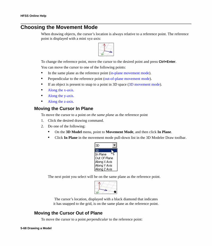


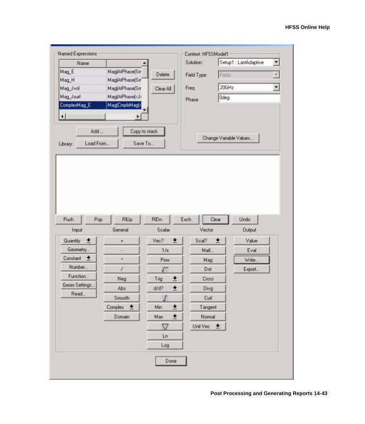


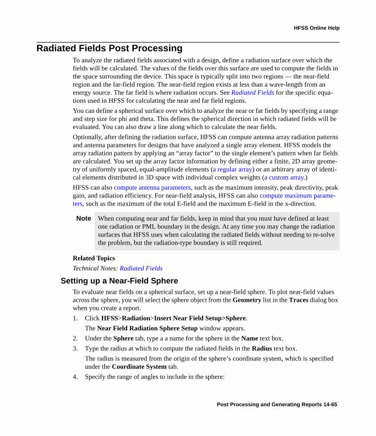


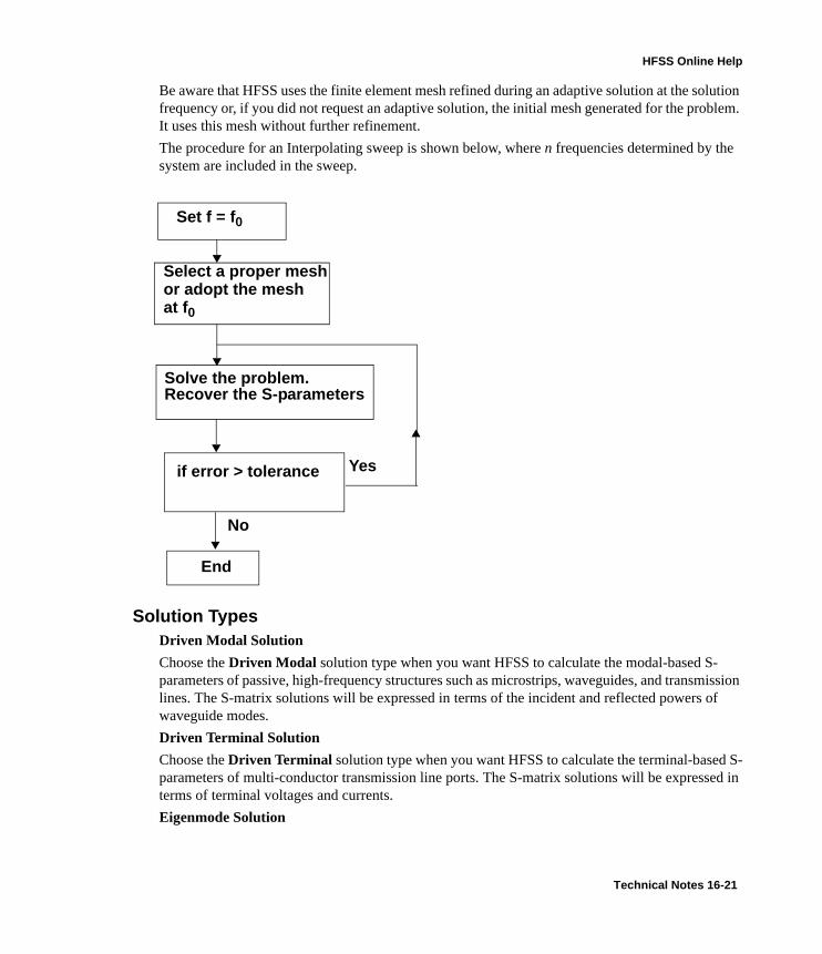


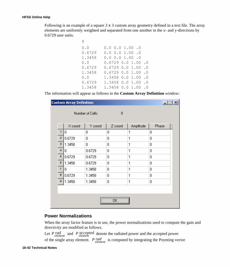


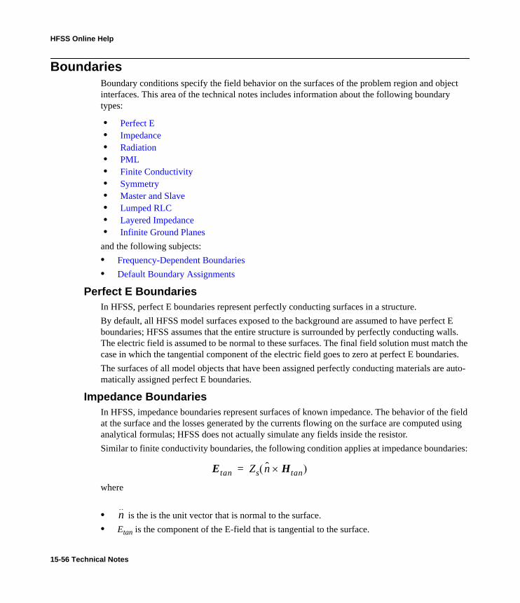


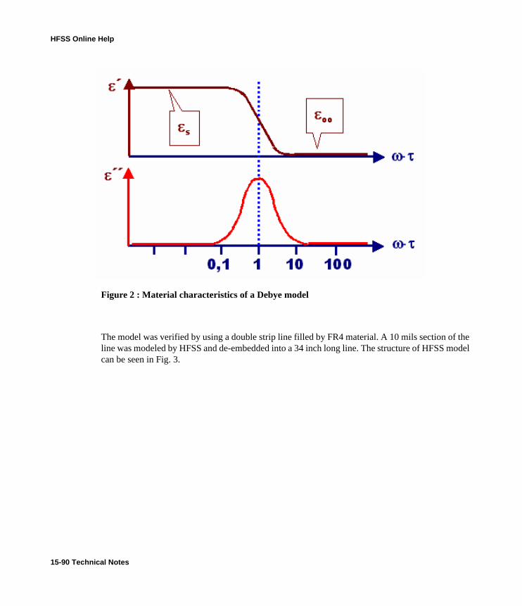


![HFSS tutorial[2nd draft] - emlab.uiuc. ?· ANSYS HFSS is an industry standard tool for simulating 3-D…](https://static.documents.pub/doc/80x56/5d17ed7888c9933b0b8bce20/hfss-tutorial2nd-draft-emlabuiuc-ansys-hfss-is-an-industry-standard-tool.jpg)


