Hidden Markov Models

By Parisa Abedi

Slides courtesy: Eric Xing

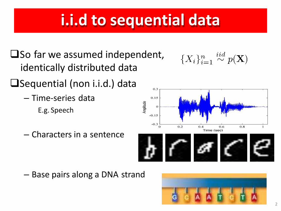
i.i.d to sequential data

So far we assumed independent, identically distributed data

Sequential (non i.i.d.) data

– Time-series data E.g. Speech

– Characters in a sentence

– Base pairs along a DNA strand

2

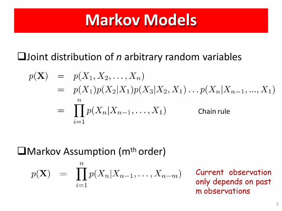
Markov Models

Joint distribution of n arbitrary random variables

Markov Assumption (mth order)

Current observation only depends on past m observations

3

Chain rule

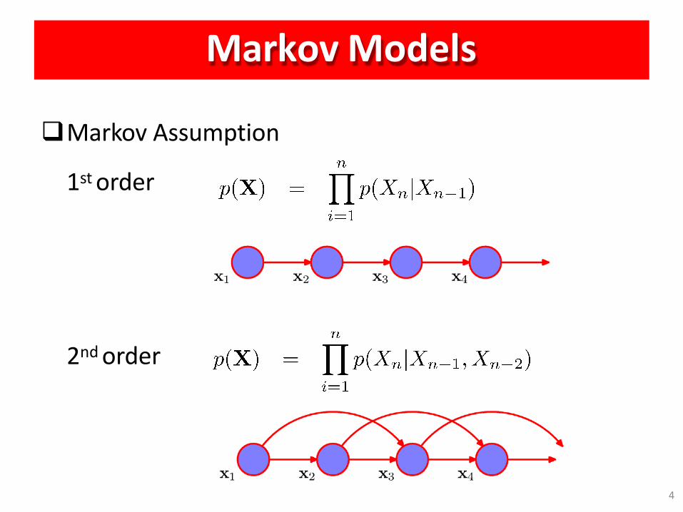
Markov Models

Markov Assumption

1st order

2nd order

4

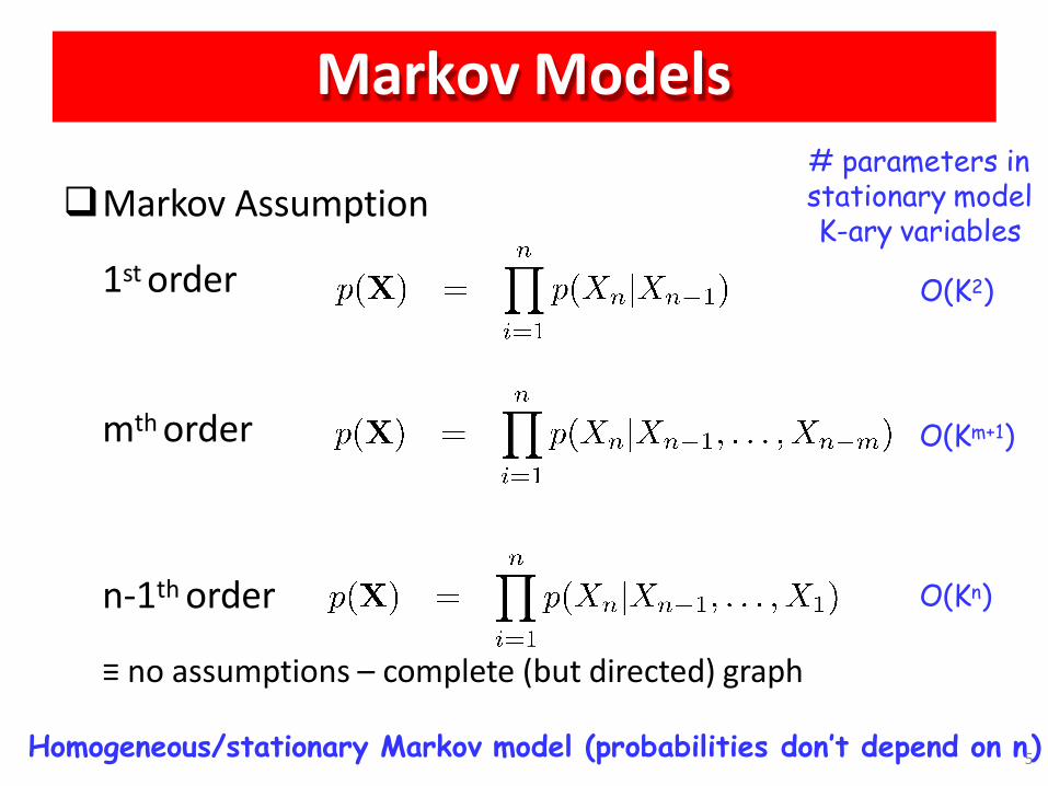
Markov Models

Markov Assumption

1st order

mth order

n-1th order

≡ no assumptions – complete (but directed) graph

# parameters in stationary model K-ary variables

O(K2)

O(Km+1)

O(Kn)

Homogeneous/stationary Markov model (probabilities don’t depend on n5)

Hidden Markov Models

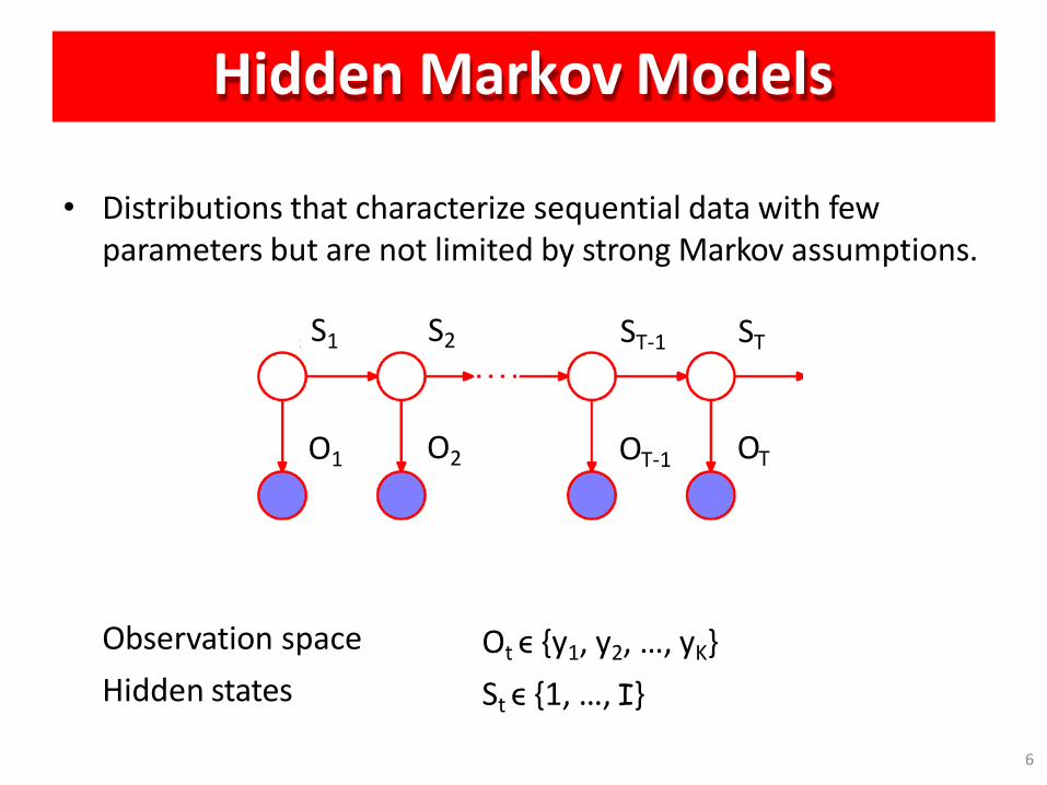
• Distributions that characterize sequential data with few parameters but are not limited by strong Markov assumptions.

Observation space

Hidden states

Ot ϵ {y1, y2, …, yK}

St ϵ {1, …, I}

O1 O2 OT-1 OT

S1 S2 ST-1 ST

6

Hidden Markov Models

O1 O2 OT-1 OT

S1 S2 ST-1 ST

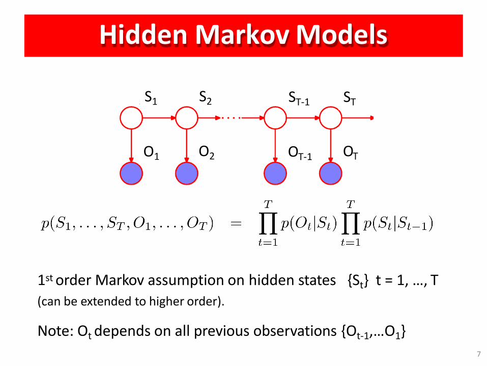
1st order Markov assumption on hidden states {St} t = 1, …, T

(can be extended to higher order).

Note: Ot depends on all previous observations {Ot-1,…O1}

7

Hidden Markov Models

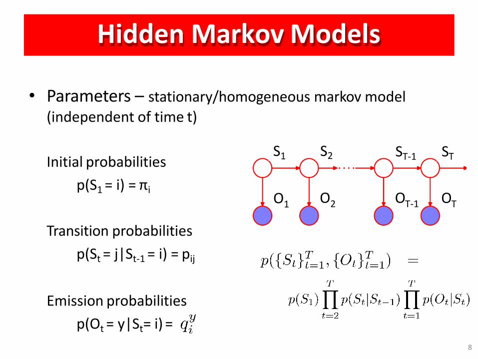
• Parameters – stationary/homogeneous markov model

(independent of time t)

Initial probabilities

p(S1 = i) = πi

Transition probabilities

p(St = j|St-1 = i) = pij

Emission probabilities

p(Ot = y|St= i) =

O 1 O 2 O T-1 O T

S1 S2 ST-1 ST

8

HMM Example

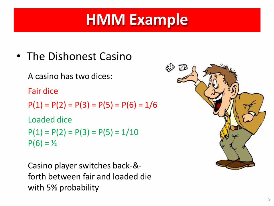
• The Dishonest Casino

A casino has two dices:

Fair dice

P(1) = P(2) = P(3) = P(5) = P(6) = 1/6

Loaded dice

P(1) = P(2) = P(3) = P(5) = 1/10 P(6) = ½

Casino player switches back-&- forth between fair and loaded die with 5% probability

9

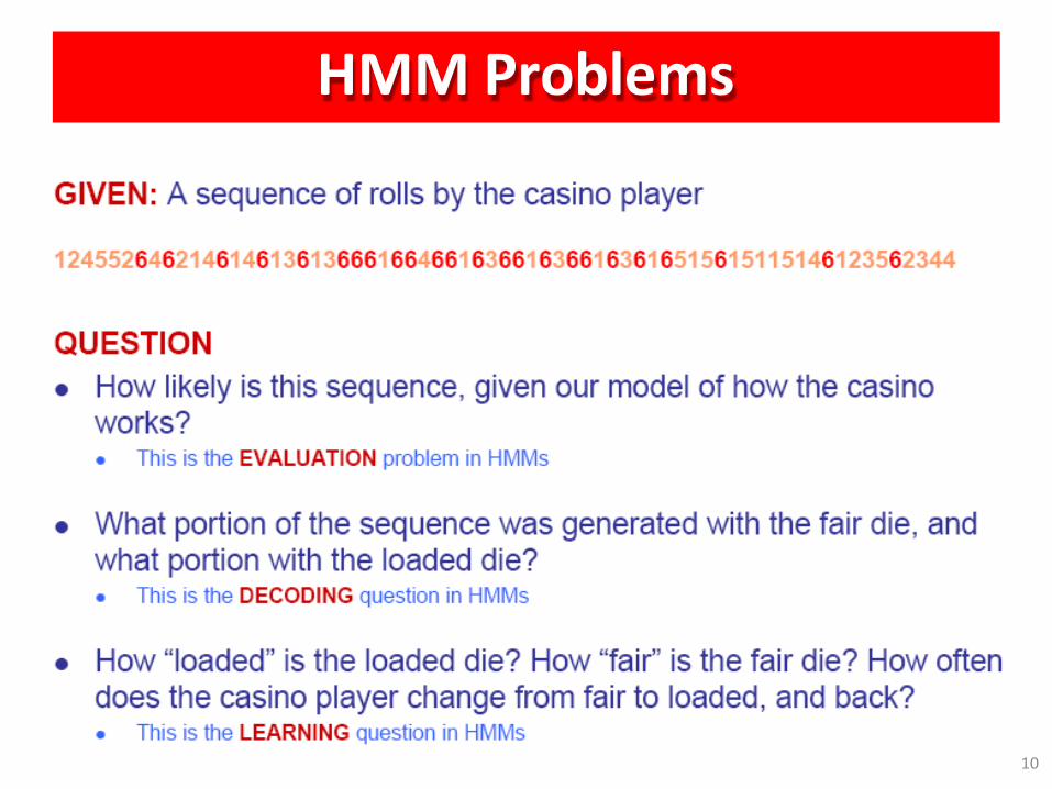
HMM Problems

10

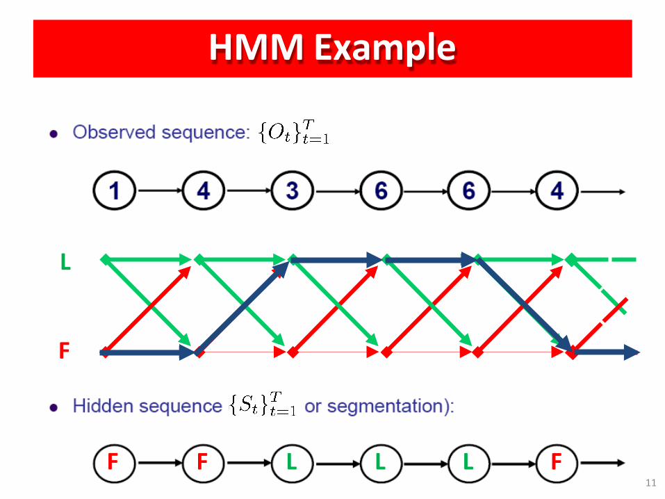
HMM Example

F F F L L L

L

F

11

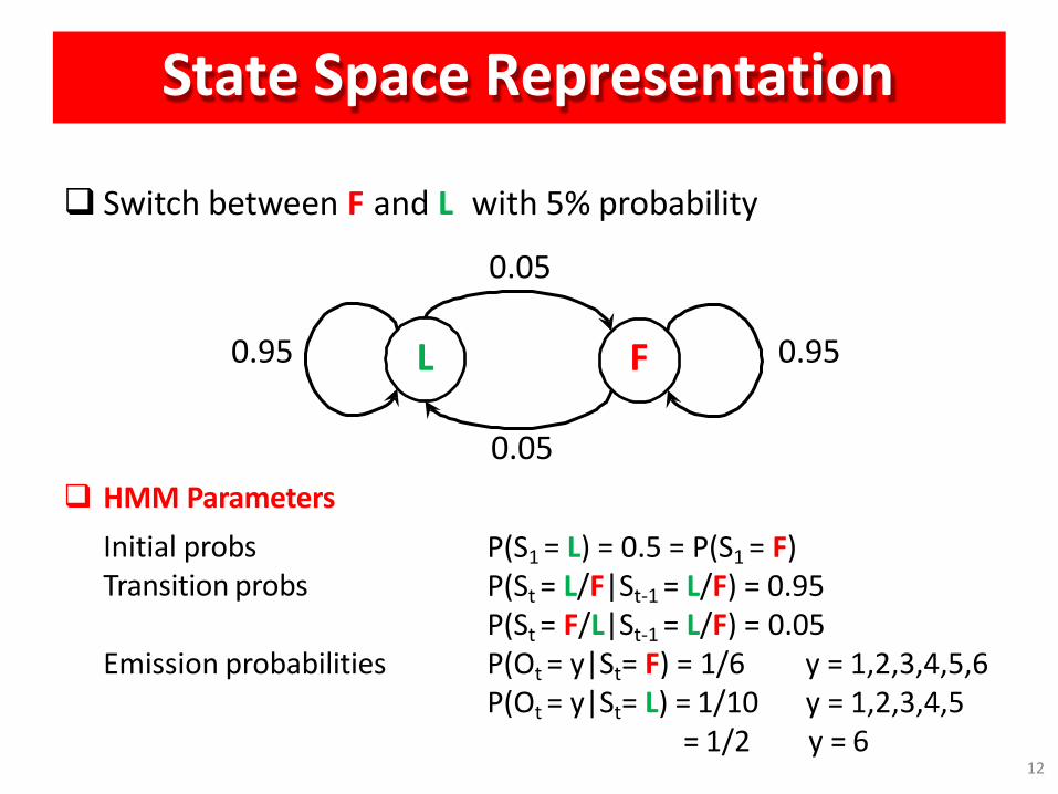
State Space Representation

HMM Parameters

Initial probs Transition probs

P(S1 = L) = 0.5 = P(S1 = F) P(St = L/F|St-1 = L/F) = 0.95 P(St = F/L|St-1 = L/F) = 0.05

Emission probabilities P(Ot = y|St= F) = 1/6 P(Ot = y|St= L) = 1/10

= 1/2

y = 1,2,3,4,5,6 y = 1,2,3,4,5 y = 6

L F

Switch between F and L with 5% probability

0.05

12

0.05

0.95 0.95

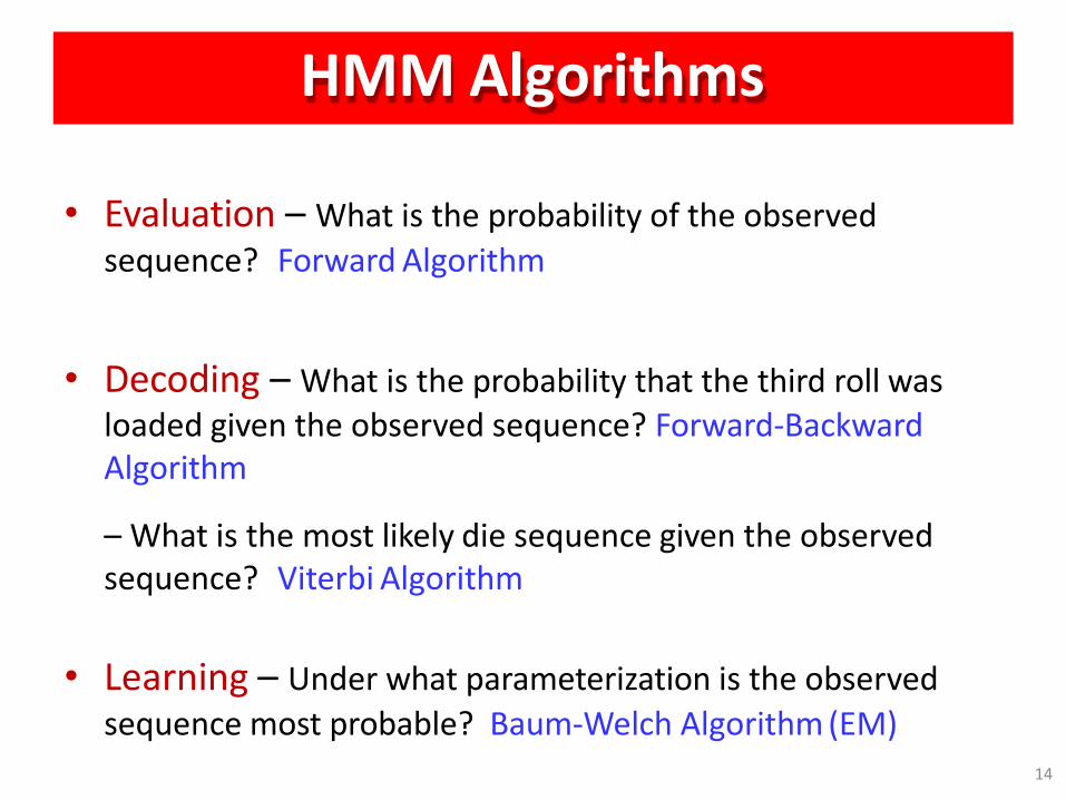
HMM Algorithms

14

• Evaluation – What is the probability of the observed

sequence? Forward Algorithm

• Decoding – What is the probability that the third roll was loaded given the observed sequence? Forward-Backward Algorithm

– What is the most likely die sequence given the observed sequence? Viterbi Algorithm

• Learning – Under what parameterization is the observed

sequence most probable? Baum-Welch Algorithm (EM)

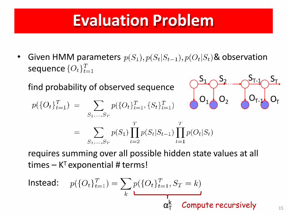
Evaluation Problem

& observation • Given HMM parameters sequence

find probability of observed sequence

requires summing over all possible hidden state values at all times – KT exponential # terms!

Instead:

αT k Compute recursively

O1 O2 OT-1 OT

S1 S2 ST-1 ST

15

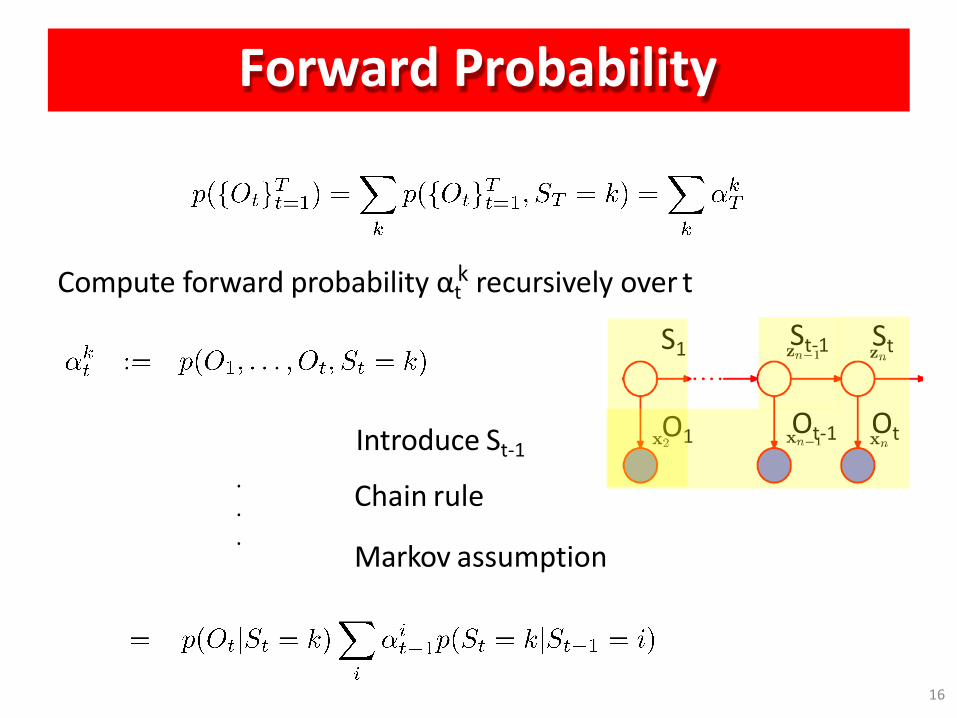
Forward Probability

Compute forward probability αt recursively over t k

.

.

. Markov assumption

Introduce St-1

Chain rule

St-1 St S1

O1 Ot-1 Ot

16

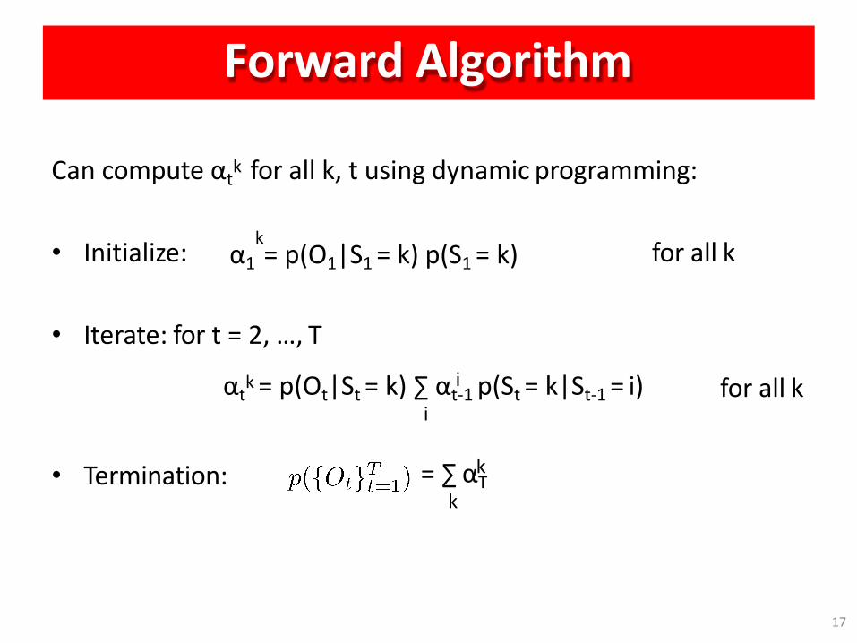
Forward Algorithm

Can compute αtk for all k, t using dynamic programming:

• Initialize: k

α1 = p(O1|S1 = k) p(S1 = k) for all k

• Iterate: for t = 2, …, T

for all k

• Termination:

i αtk = p(Ot|St = k) ∑ αt-1 p(St = k|St-1 = i)

i

= ∑ αT k

17

k

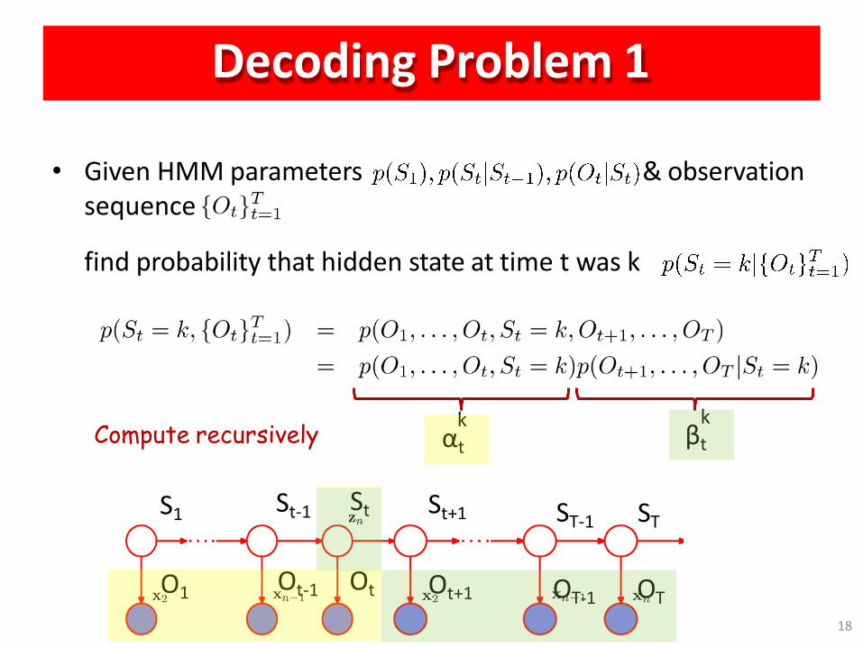
Decoding Problem 1

& observation • Given HMM parameters sequence

find probability that hidden state at time t was k

k αt

Compute recursively k

βt

St-1 St S1

O1 Ot-1 Ot

ST-1 ST St+1

Ot+1 OT-1 OT

18

ST

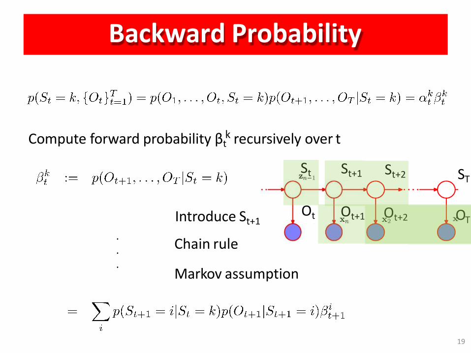
Backward Probability

Compute forward probability βt recursively over t k

.

.

. Markov assumption

Ot

St St+1 St+2

Ot+1 Ot+2 OT Introduce St+1

Chain rule

19

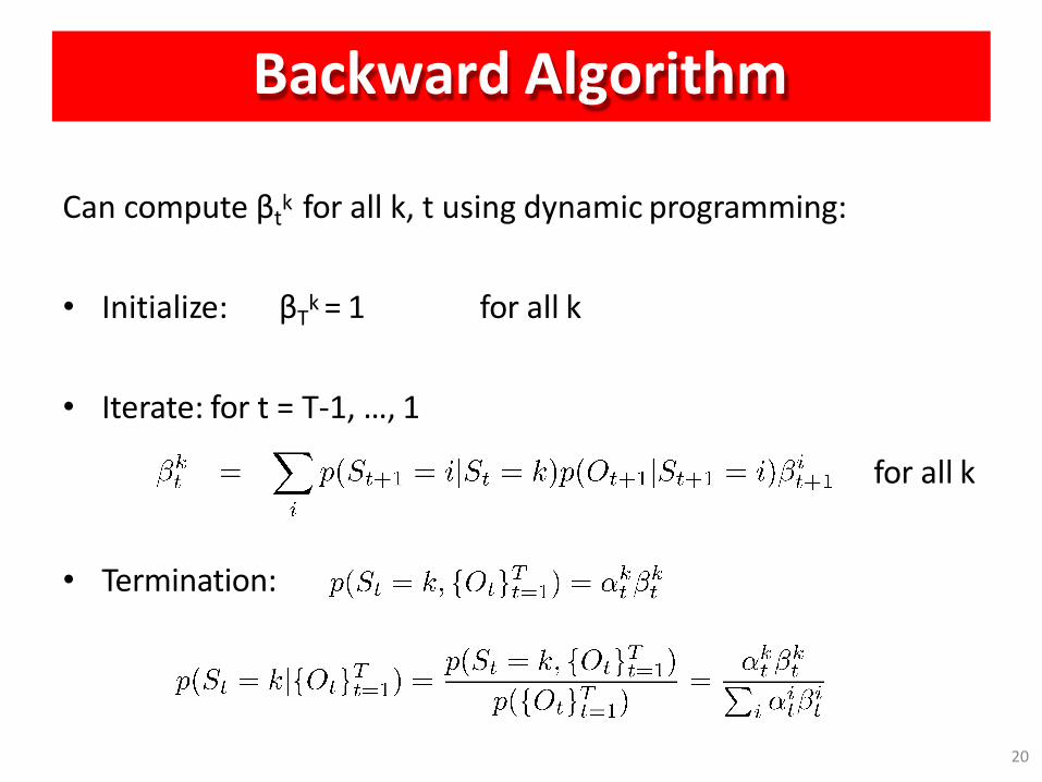
Backward Algorithm

Can compute βtk for all k, t using dynamic programming:

• Initialize: βTk = 1 for all k

• Iterate: for t = T-1, …, 1

for all k

• Termination:

20

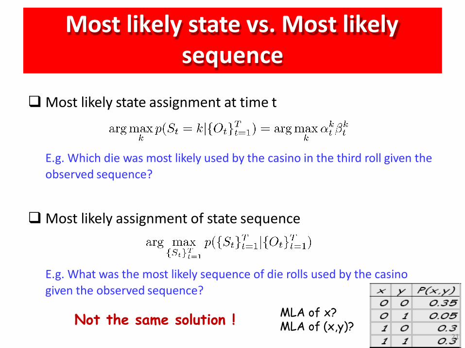
Most likely state vs. Most likely sequence

Most likely state assignment at time t

E.g. Which die was most likely used by the casino in the third roll given the

observed sequence?

Most likely assignment of state sequence

E.g. What was the most likely sequence of die rolls used by the casino

given the observed sequence?

Not the same solution ! MLA of x? MLA of (x,y)?

21

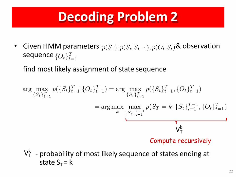
Decoding Problem 2

& observation • Given HMM parameters sequence

find most likely assignment of state sequence

VT

22

k

Compute recursively

- probability of most likely sequence of states ending at state ST = k

VT k

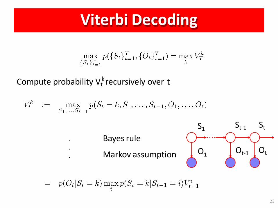
Viterbi Decoding

.

.

.

Bayes rule

Markov assumption

Compute probability Vt recursively over t k

Ot-1 Ot

St-1 St S1

O

23

1

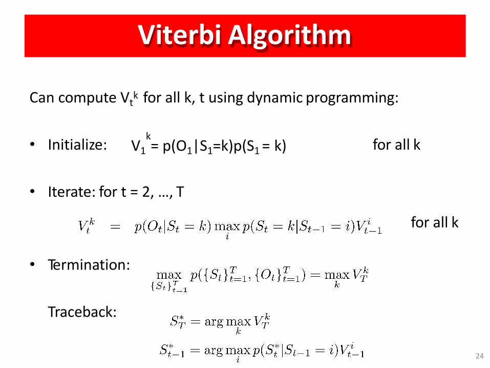
Viterbi Algorithm

Can compute Vtk for all k, t using dynamic programming:

• Initialize: k

V1 = p(O1|S1=k)p(S1 = k) for all k

• Iterate: for t = 2, …, T

for all k

• Termination:

Traceback:

24

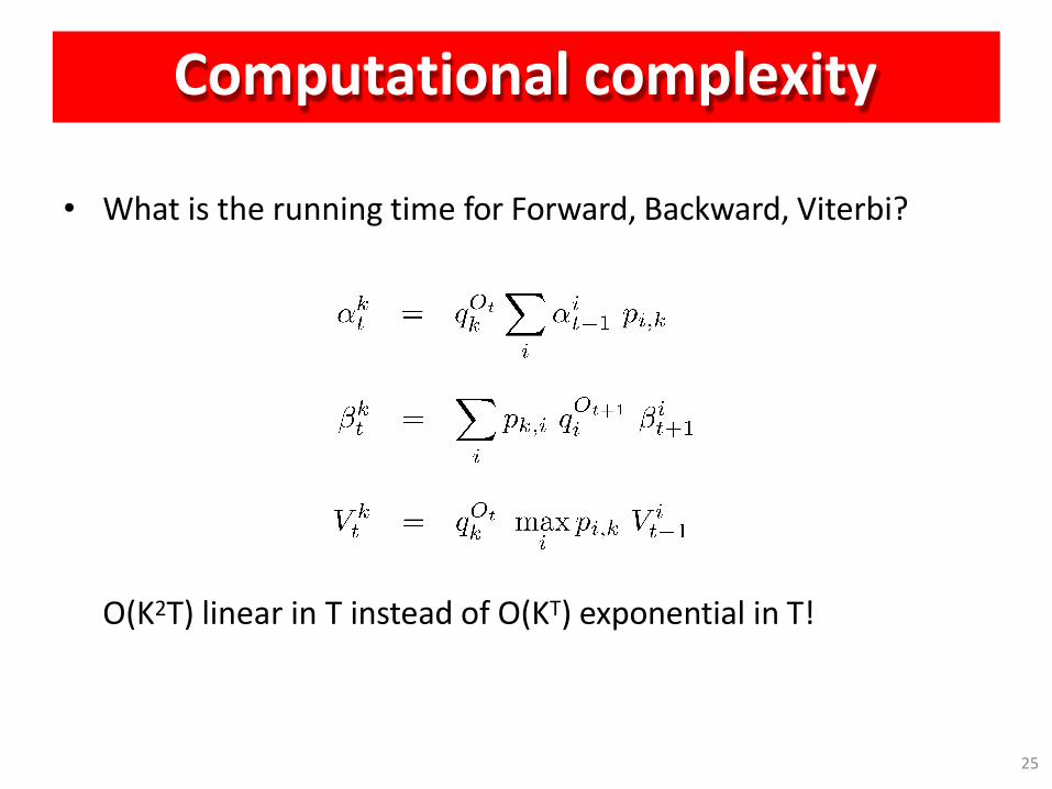
Computational complexity

• What is the running time for Forward, Backward, Viterbi?

O(K2T) linear in T instead of O(KT) exponential in T!

25

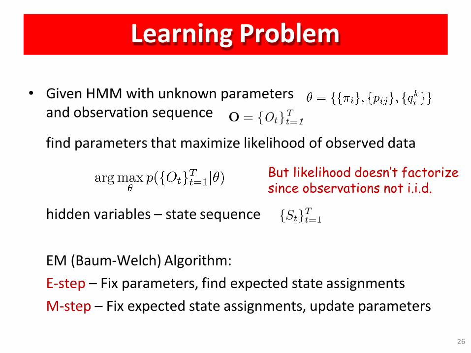
Learning Problem

• Given HMM with unknown parameters and observation sequence

find parameters that maximize likelihood of observed data

But likelihood doesn’t factorize since observations not i.i.d.

hidden variables – state sequence

EM (Baum-Welch) Algorithm:

E-step – Fix parameters, find expected state assignments

M-step – Fix expected state assignments, update parameters

26

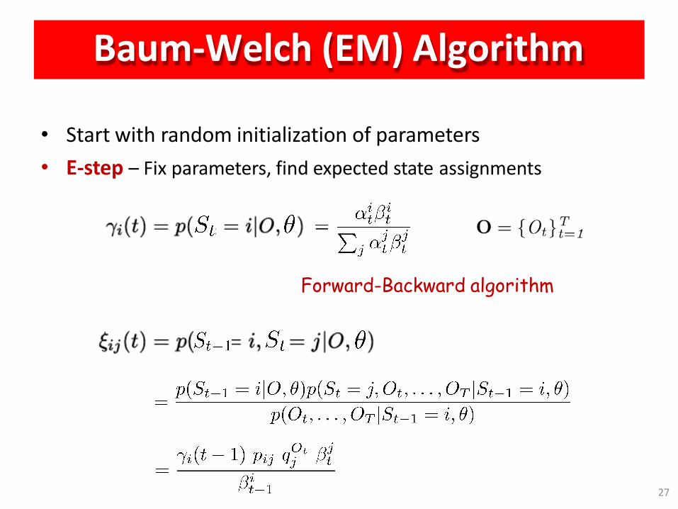
Baum-Welch (EM) Algorithm

• Start with random initialization of parameters

• E-step – Fix parameters, find expected state assignments

Forward-Backward algorithm

27

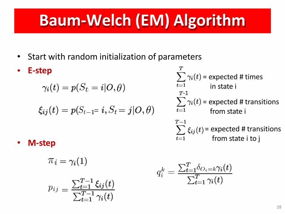
Baum-Welch (EM) Algorithm

• Start with random initialization of parameters

• E-step

• M-step

= expected # transitions from state i to j

= expected # times in state i

= expected # transitions from state i

28

-1

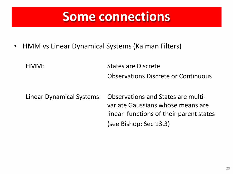
Some connections

29

• HMM vs Linear Dynamical Systems (Kalman Filters)

HMM: States are Discrete

Observations Discrete or Continuous

Linear Dynamical Systems: Observations and States are multi- variate Gaussians whose means are linear functions of their parent states

(see Bishop: Sec 13.3)

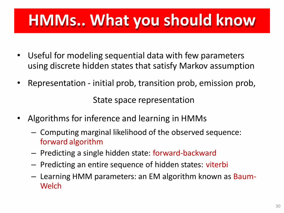
HMMs.. What you should know

30

• Useful for modeling sequential data with few parameters using discrete hidden states that satisfy Markov assumption

• Representation - initial prob, transition prob, emission prob,

State space representation

• Algorithms for inference and learning in HMMs

– Computing marginal likelihood of the observed sequence: forward algorithm

– Predicting a single hidden state: forward-backward

– Predicting an entire sequence of hidden states: viterbi

– Learning HMM parameters: an EM algorithm known as Baum- Welch