Technische Mechanik, Band 24, Heft 3-4, (2004), 242-253 Manuskripteingang: 19. April 2004 High-Order Sub-Harmonic Synchronisation in a Rotor System with a Gear Coupling E. Brommundt Dedicated to the memory of Professor Friedrich Rimrott Gear couplings transmit torque from driving to driven shafts whilst accommodating unavoidable misalignments and axial displacements. The friction forces at the sliding teeth transfer energy from the driving engine to the lateral oscillations of the shaft. Instability of the stationary motion, self-excitation, can result. The self-excited oscillations, in character related to the eigen-oscillations of the linear system, interact with the external excita- tion by unbalance forces. For a two degrees of freedom rotor-bearing system we show how to study systemati- cally cases of higher-order synchronisation (frequency locking) which can help to interpret observed motions; numerical calculations and perturbation techniques are combined. 1 Introduction Gear couplings consist of an externally toothed hub, see Fig.1a, and a mating sleeve with internal teeth which permit relative axial sliding. Crowning (rounding) of the hub teeth and a clearance (backlash) between the mesh- ing gears prevent jamming and allow small angular displacements (angular misalignments) between the axes of sleeve and hub (see the angle α in Fig.1b; | | α < 0.004 rad ≈ 0.25° at high speeds). The incorporation of the gear coupling into a rotor-bearing system has unwel- come side effects: The touching teeth-flanks need some slipping for lubrication, thus a minimum misalignment | | α > 0 is necessary. The Coulomb type friction forces between the sliding tooth flanks introduce strictly non- linear effects into the otherwise linear rotor system. Like a shaft with internal friction (Ku et al., 1993) – rotating with an angular speed – a rotor with a gear coupling will start to oscillate at a frequency as soon as Ω r ω Ω exceeds As a rule, the r . ω r elevant frequency r ω is close to the natural frequency of that (linear) modal oscilla- tion which draws most effectively energy from the power supply. Both, linear and non-linear terms of the equa- tions of motion control the energy flow into the relevant mode and determine the amplitudes of the self- oscillation (of course, this depends on several system parameters). The frequency r ω remains about fixed when increases further, the self-oscillation appears as a sub-harmonic oscillation. (Sub-harmonic in contrast to the harmonic oscillations – at the frequency – forced by the unbalances of the rotor.) In this paper we study the interaction of these two types of oscillation in a simple rotor system. Ω Ω α T TR TL M M M = ≈ Fig. 1: Gear coupling; a) straight, b) displaced by angle with moments applying to the left half, The bulk of literature on rotor systems with gear couplings concentrates on coupling alignment, lubrication and wear; e.g. Piotrowski (1995). Most of these publications contain no details about the vibrations which certainly accompany wear. A few authors report about instability and self-excited oscillations observed in plants; e.g. Shiraki et al. (1970). Common to all cases are the rather sudden onset of vibrations when the rotational speed of the rotor is increased, and the sub-synchronous frequency of the observed (self-excited) oscillations, independent of the speed Ω Not all authors seem to identify the gear coupling as source of their trouble. Little literature exists on systematic investigations of self-excitation by gear couplings. Morton (1982) demonstrates by a four degrees of freedom rotor that a sufficiently large angular displacement of the coupling stabilizes the system; Yamauchi et al. (1981) study the dynamic characteristics of gear couplings analytically and experimentally. . The model of this paper is taken from Brommundt et al. (in preparation), where additional literature is listed. We use that model here to show how intricate oscillations, somewhat hidden in parameter space, can be uncovered by numerical means supported by perturbation techniques. 242
Transcript
Technische Mechanik, Band 24, Heft 3-4, (2004), 242-253 Manuskripteingang: 19. April 2004
High-Order Sub-Harmonic Synchronisation in a Rotor System with a Gear Coupling E. Brommundt Dedicated to the memory of Professor Friedrich Rimrott Gear couplings transmit torque from driving to driven shafts whilst accommodating unavoidable misalignments and axial displacements. The friction forces at the sliding teeth transfer energy from the driving engine to the lateral oscillations of the shaft. Instability of the stationary motion, self-excitation, can result. The self-excited oscillations, in character related to the eigen-oscillations of the linear system, interact with the external excita-tion by unbalance forces. For a two degrees of freedom rotor-bearing system we show how to study systemati-cally cases of higher-order synchronisation (frequency locking) which can help to interpret observed motions; numerical calculations and perturbation techniques are combined. 1 Introduction Gear couplings consist of an externally toothed hub, see Fig.1a, and a mating sleeve with internal teeth which permit relative axial sliding. Crowning (rounding) of the hub teeth and a clearance (backlash) between the mesh-
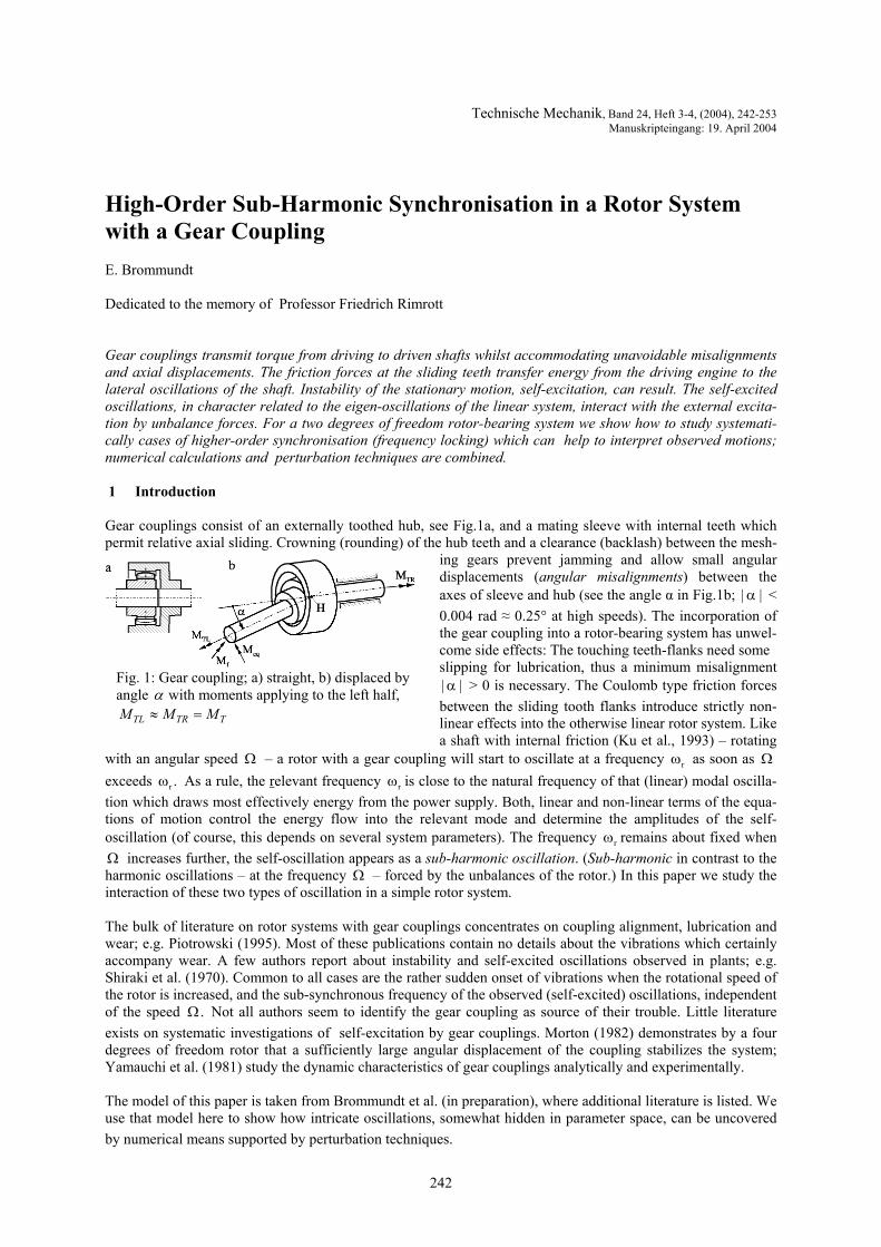
ing gears prevent jamming and allow small angular displacements (angular misalignments) between the axes of sleeve and hub (see the angle α in Fig.1b; | |α < 0.004 rad ≈ 0.25° at high speeds). The incorporation of the gear coupling into a rotor-bearing system has unwel-come side effects: The touching teeth-flanks need some slipping for lubrication, thus a minimum misalignment
|| α > 0 is necessary. The Coulomb type friction forces between the sliding tooth flanks introduce strictly non-linear effects into the otherwise linear rotor system. Like a shaft with internal friction (Ku et al., 1993) – rotating
with an angular speed – a rotor with a gear coupling will start to oscillate at a frequency as soon as Ω rω Ω exceeds As a rule, the r .ω relevant frequency rω is close to the natural frequency of that (linear) modal oscilla-tion which draws most effectively energy from the power supply. Both, linear and non-linear terms of the equa-tions of motion control the energy flow into the relevant mode and determine the amplitudes of the self-oscillation (of course, this depends on several system parameters). The frequency rω remains about fixed when
increases further, the self-oscillation appears as a sub-harmonic oscillation. (Sub-harmonic in contrast to the harmonic oscillations – at the frequency – forced by the unbalances of the rotor.) In this paper we study the interaction of these two types of oscillation in a simple rotor system.
ΩΩ
αTTRTL MMM =≈
Fig. 1: Gear coupling; a) straight, b) displaced byangle with moments applying to the left half,
The bulk of literature on rotor systems with gear couplings concentrates on coupling alignment, lubrication and wear; e.g. Piotrowski (1995). Most of these publications contain no details about the vibrations which certainly accompany wear. A few authors report about instability and self-excited oscillations observed in plants; e.g. Shiraki et al. (1970). Common to all cases are the rather sudden onset of vibrations when the rotational speed of the rotor is increased, and the sub-synchronous frequency of the observed (self-excited) oscillations, independent of the speed Ω Not all authors seem to identify the gear coupling as source of their trouble. Little literature exists on systematic investigations of self-excitation by gear couplings. Morton (1982) demonstrates by a four degrees of freedom rotor that a sufficiently large angular displacement of the coupling stabilizes the system; Yamauchi et al. (1981) study the dynamic characteristics of gear couplings analytically and experimentally.
.
The model of this paper is taken from Brommundt et al. (in preparation), where additional literature is listed. We use that model here to show how intricate oscillations, somewhat hidden in parameter space, can be uncovered by numerical means supported by perturbation techniques.
242
2 The Basics of Our System 2.1 The System
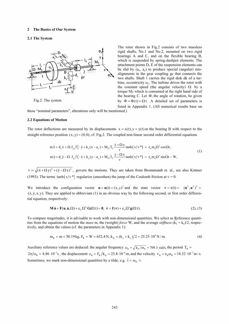
The rotor shown in Fig.2 consists of two massless rigid shafts, No.1 and No.2, mounted on two rigid bearings A and C, and on the flexible bearing B, which is suspended by spring-dashpot elements. The attachment points D, E of the suspension elements can be slid by (ax, ay) to produce special (angular) mis-alignments in the gear coupling gc that connects the two shafts. Shaft 1 carries the rigid disk dk of a tur-bine, eccentricity eU. The turbine drives the rotor with the constant speed (the angular velocity) by a torque M
ΩT which is consumed at the right hand side of
the bearing C. Let ,Φ the angle of rotation, be given by (t) t.Φ = Φ = Ω A detailed set of parameters is listed in Appendix 1. (All numerical results base on
these “nominal parameters”, alterations only will be mentioned.)
Fig.2: The system
2.2 Equations of Motion The rotor deflections are measured by its displacements x x(t), y y(t)= = at the bearing B with respect to the straight reference position (x cf. Fig.2. The coupled non-linear second order differential equations , y) (0,0),=
( )
( )
2 2x p 2 x x F 2 u u
2 2y p 2 y y F 2 u u
x ym x d x J l y k (x a ) M l tanh v v * e m cos t ,v
y xm y d y J l x k (y a ) M l tanh v v * e m sin t W,v
+Ω+ + Ω ⋅ + − + = Ω Ω
−Ω+ −Ω ⋅ + − + = Ω Ω −
&&& & &
&&& & &
(1)
2v : (x y) (y x) ,= +Ω + −Ω& & 2 govern the motions. They are taken from Brommundt et. al., see also Krämer
(1993). The terms ( )tanh v v * regularize (smoothen) the jump of the Coulomb friction at v = 0. We introduce the configuration vector and the state vector T(t) (x, y)= =u u (t)= =v v T T T( , ) =u u&
They are applied to abbreviate (1) in an obvious way by the following second, or first order differen-tial equation, respectively: (x, y,x, y).& &
(2), (3) 2
U( , , ) e t) , ( ) e ( t).+ Ω + Ω Ω = = + Ω ΩM u F u u G( 0 v f v g&& & & 2U
To compare magnitudes, it is advisable to work with non-dimensional quantities. We select as Reference quanti-ties from the equations of motion the mass m, the (weight) force W, and the average stiffness (kx + ky)/2, respec-tively, and obtain the values (cf. the parameters in Appendix 1): 6
R R R x ym m 50.19kg, F W 652.4 N, k (k k ) 2 25.25 10 N / m.= = = = = + = ⋅ (4) Auxiliary reference values are deduced: the angular frequency R R Rk m 709.3 rad/s,= ⋅ω = the period TR =
3R2 8.86 10−π ω = ⋅ s , the displacement 6
R R Re F k 25.8 10 m−= = ⋅ ,
.
and the velocity
Sometimes, we mark non-dimensional quantities by a tilde, e.g.
3R R Rv e 18.32 10 m / s.−= ω = ⋅
Rt t= ω ⋅%
243
2.3 Solutions for the Linear System To become acquainted with our system we ask for its “linear behaviour” without the influence of the gear cou-pling effects, i.e. for MF = 0 in (1): The free vibrations (5) exp( t)= λu u(
are two (couples of complex conjugate) eigen-solutions ( , k)λ u( , k k kj ,λ = σ + ω k = 1, 2, ( j := √ (-1) ). Because
of the gyroscopic effect they depend on the speed .Ω Here are values for R 0.0, 1.0, 2.0, 3.0:ω =/Ω = Ω%
T
R 1 R 1 RT
2 R 2 RT
R 1 R 1 RT
2 R 2 RT
R 1 R 1 R
0.0: 0.039 0.895j, e (1, 0),
0.064 1.093j, e (0, 1);
1.0: 0.040 0.885j, e (1, 0.013 0.208j),
0.064 1.105j, e (0.018 0.254 j, 1);
2.0: 0.040 0.860 j, e
Ω ω = λ ω = − + =
λ ω = − + =
Ω ω = λ ω = − + = +
λ ω = − + = +
Ω ω = λ ω = − + =
u
u
u
u
u
(
(
(
(
(
T2 R 2 R
TR 1 R 1 R
T2 R 2 R
(1, 0.017 0.366 j),
0.064 1.137 j, e (0.026 0.447 j, 1);
3.0: 0.039 0.828j, e (1, 0.017 0.474 j),
0.065 1.181j, e (0.027 0.579 j, 1).
+
λ ω = − + = +
Ω ω = λ ω = − + = +
λ ω = − + = +
u
u
u
(
(
(
(6)
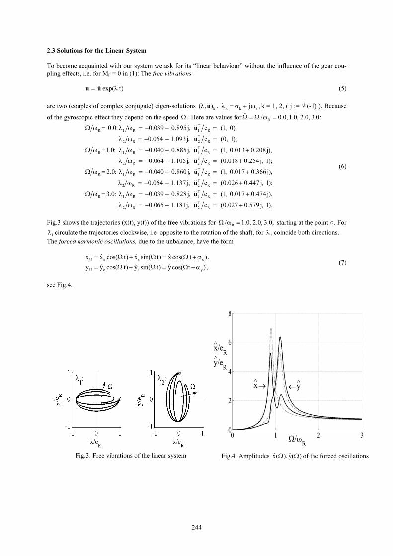
Fig.3 shows the trajectories (x(t), y(t)) of the free vibrations for R/ 1.0, 2.0, 3.0,Ω ω =
2
starting at the point . For circulate the trajectories clockwise, i.e. opposite to the rotation of the shaft, for 1λ λ coincide both directions.
The forced harmonic oscillations, due to the unbalance, have the form
(7) U c s x
U c s y
ˆ ˆ ˆx x cos( t) x sin( t) x cos( t ) ,ˆ ˆ ˆy y cos( t) y sin( t) ycos( t ) ,
= Ω + Ω = Ω +α= Ω + Ω = Ω +α
see Fig.4.
ˆ ˆx( ), y( )Ω ΩFig.4: Amplitudes of the forced oscillationsFig.3: Free vibrations of the linear system
244
3 The Behaviour of the Perfectly Balanced System Perfect balance means eU = 0 in (1). Furthermore, we assume ax = 0 and sum the effects of the weight W and the adjustment ay. Their combined action is captured by the parameter ma (it steers the misalignment): (8) a ym W W a k .= − y
Then, equation (1) gets the form
( )
( )
2x p 2 x F 2
2y p 2 y F 2 a
x ym x d x J l y k x M l tanh v v * 0,v
y xm y d y J l x k y M l tanh v v * m W.v
+Ω+ + Ω ⋅ + + =
−Ω+ −Ω ⋅ + + = −
&&& & &
&&& & &
(9)
3.1 The Stationary Solution and its Stability The autonomous equation (9) has the stationary solution (10) T
0 0 0(x , y ) ( cos , sin ) ,= = ρ γ −ρu γ where ρ and γ follow from
( )( ) ( )
( )
2 22 2 2x y F 2 x F 2 a
x F 2
k k (M / l ) tanh( /v*) k (M / l ) tanh( /v*) m W,
tan k (M / l ) tanh( /v*) .
ρ + Ωρ ρ + Ωρ =
γ = ρ Ωρ (11)
To investigate the stability of u0 it is disturbed by δu, and the behaviour of perturbed solution u = u0 + δu is obtained from the variational equation, cf. (1) and (2), (12) 0 0( , , ) ( , , ) ,δ + Ω δ + Ω δ =u uM u F u 0 u F u 0 u 0&&& &
where and are Jacobi matrices of F with respect to and u at the constant displacement uuF& uF u& 0 (the details
are a bit lengthy). The displacement u0 is stable (with respect to sufficiently small perturbations) when all eigen-solutions
exp( t)δ = λu u) decay, i.e., when .k k: Re 0, for k 1,..., 4σ = λ < =
As an example, Fig.5 demonstrates some results calculated for – nominal speed. Fig.5a shows the stationary displacement (x0, y0) of the bearing B as it changes when ma is increased from 0 to 6: the suspension point E of the (initially
weightless) rotor is shifted from zero to a value equivalent to a rotor displacement caused by a 6-fold weight. (The bullet at (x0, y0) ≈ (0, 0) holds for ma = 1 where the coupling nearly sticks.) Fig.5b sh max ,σ the largest real-part of the eigen-values, as function
N N;Ω
ts u0.)
0.5Ω = ⋅Ω
ows of ma. Except for the small gap between ma1 = 1.05 and ma2 = 1.28,
maxσ is positive up to ma3 = 2.93. Throughout the region 0 < ma < ma3 the stationary displacement is unstable. (A careful study of the stable stationary solution within the gap between ma1 and ma2 reveals that it has a very small domain of attraction only: any not so small disturbance upse
maxσFig.5: Stationary solution; a) displacement, b) real-part
Remark 1: Here, a value ma > 3 stabilises the stationary displacement. An ma = 3 leads to an angle α of less than 0.1º (cf. the Introduction). Thus, an appropriately chosen ma seems to be a remedy against instability, generally applicable. But the magnitude of ma is limited by the heat generation in the coupling (cf. Czerny, 1993)!
245
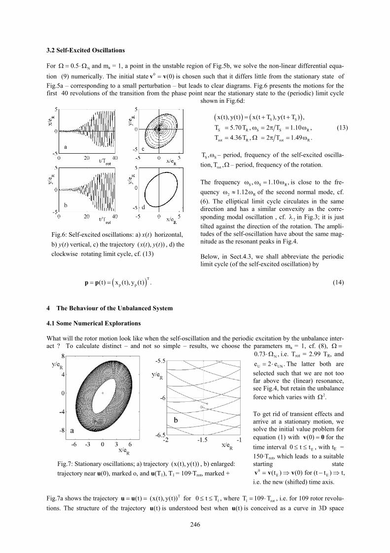
3.2 Self-Excited Oscillations For and mN0.5Ω = ⋅Ω a = 1, a point in the unstable region of Fig.5b, we solve the non-linear differential equa-tion (9) numerically. The initial state is chosen such that it differs little from the stationary state of Fig.5a – corresponding to a small perturbation – but leads to clear diagrams. Fig.6 presents the motions for the first 40 revolutions of the transition from the phase point near the stationary state to the (periodic) limit cycle
shown in Fig.6d:
0 (0)=v v
( )x t( )y t ( ( ), ( ))x t y t
Fig.6: Self-excited oscillations: a) horizontal, b) vertical, c) the trajectory , d) the clockwise rotating limit cycle, cf. (13)
( ) ( )S S
S R S S
rot R rot R
x(t), y(t) x(t T ), y(t T ) ,T 5.70T , 2 T 1.10T 4.36T , 2 T 1.49
= + +
R
.,= ω = π = ω
= Ω = π = ω (13)
ST , Sω – period, frequency of the self-excited oscilla-
tion, rotT ,Ω – period, frequency of the rotation. The frequency S S, 1.10 R,ω ω = ω
2 R1.12is close to the fre-
quency ω ≈ ω of the second normal mode, cf. (6). The elliptical limit cycle circulates in the same direction and has a similar convexity as the corre-sponding modal oscillation , cf. in Fig.3; it is just tilted against the direction of the rotation. The ampli-tudes of the self-oscillation have about the same mag-nitude as the resonant peaks in Fig.4.
2λ
Below, in Sect.4.3, we shall abbreviate the periodic limit cycle (of the self-excited oscillation) by
(14) ( T
p p(t) x (t), y (t) .= =p p ) 4 The Behaviour of the Unbalanced System 4.1 Some Numerical Explorations What will the rotor motion look like when the self-oscillation and the periodic excitation by the unbalance inter-act ? To calculate distinct – and not so simple – results, we choose the parameters ma = 1, cf. (8), Ω =
N0.73 ,⋅Ω
Ue 2 ei.e. Trot = 2.99 TR, and
UN .= ⋅ The latter both are selected such that we are not too far above the (linear) resonance, see Fig.4, but retain the unbalance force which varies with Ω 2.
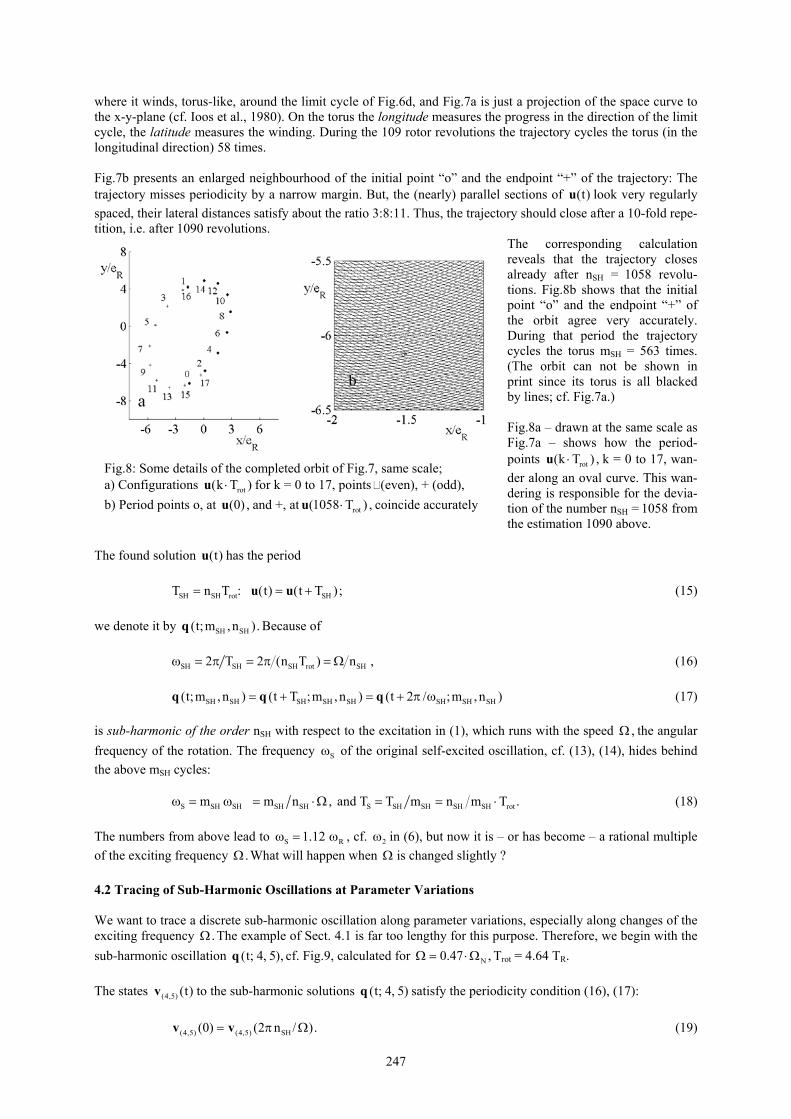
Fig.7: Stationary oscillations; a) trajectory , b) enlarged: trajectory near u(0), marked o, and u(T1), T1 = 109·Trot, marked +
(x(t), y(t))
To get rid of transient effects and arrive at a stationary motion, we solve the initial value problem for equation (1) with for the time interval 0 t , with t
(0) =v
Et≤ ≤
) for (t t
0
E = 150·Trot, which leads to a suitable starting state
i.e. the new (shifted) time axis.
0 (t ) ( ) t,= ⇒ − ⇒v v E E0v
Fig.7a shows the trajectory for (t)= =u u T(x(t), y(t)) 10 t T≤ ≤ , where t1T 109 Tro= ⋅
), i.e. for 109 rotor revolu-
tions. The structure of the trajectory is understood best when is conceived as a curve in 3D space (t)u (tu
246
where it winds, torus-like, around the limit cycle of Fig.6d, and Fig.7a is just a projection of the space curve to the x-y-plane (cf. Ioos et al., 1980). On the torus the longitude measures the progress in the direction of the limit cycle, the latitude measures the winding. During the 109 rotor revolutions the trajectory cycles the torus (in the longitudinal direction) 58 times. Fig.7b presents an enlarged neighbourhood of the initial point “o” and the endpoint “+” of the trajectory: The trajectory misses periodicity by a narrow margin. But, the (nearly) parallel sections of u look very regularly spaced, their lateral distances satisfy about the ratio 3:8:11. Thus, the trajectory should close after a 10-fold repe-tition, i.e. after 1090 revolutions.
(t)
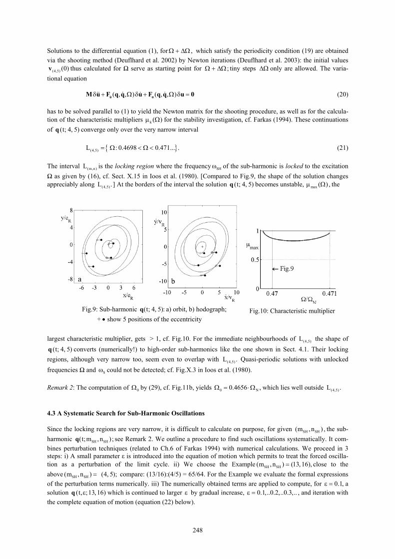
The corresponding calculation reveals that the trajectory closes already after nSH = 1058 revolu-tions. Fig.8b shows that the initial point “o” and the endpoint “+” of the orbit agree very accurately. During that period the trajectory cycles the torus mSH = 563 times. (The orbit can not be shown in print since its torus is all blacked by lines; cf. Fig.7a.) Fig.8a – drawn at the same scale as Fig.7a – shows how the period-points u k = 0 to 17, wan-der along an oval curve. This wan-dering is responsible for the devia-tion of the number n
rot(k T ) ,⋅
SH = 1058 from the estimation 1090 above.
The found solution has the period (t)u (15) SH SH rot SHT n T : (t) (t T )= = +u u ; we denote it by q Because of SH SH(t;m , n ). SH SH SH rot SH2 T 2 (n T ) nω = π = π = Ω , (16) (17) SH SH SH SH SH SH SH SH(t;m , n ) (t T ;m , n ) (t 2 / ;m , n )= + = + π ωq q q is sub-harmonic of the order nSH with respect to the excitation in (1), which runs with the speed Ω the angular frequency of the rotation. The frequency of the original self-excited oscillation, cf. (13), (14), hides behind the above m
,
Sω
SH cycles: S SH SH SH SH S SH SH SH SH rotm m n , and T T m n mω = ω = ⋅Ω = = ⋅T .
R
(18) The numbers from above lead to , cf. S 1.12ω = ω 2ω in (6), but now it is – or has become – a rational multiple of the exciting frequency .Ω What will happen when Ω is changed slightly ? 4.2 Tracing of Sub-Harmonic Oscillations at Parameter Variations We want to trace a discrete sub-harmonic oscillation along parameter variations, especially along changes of the exciting frequency .The example of Sect. 4.1 is far too lengthy for this purpose. Therefore, we begin with the sub-harmonic oscillation cf. Fig.9, calculated for
Ω(t; 4, 5),q N0.47 ,Ω = ⋅Ω Trot = 4.64 TR.
The states to the sub-harmonic solutions q satisfy the periodicity condition (16), (17): (4,5) (t)v (t; 4, 5) . (19) (4,5) (4,5) SH(0) (2 n / )= πv v Ω
Fig.8: Some details of the completed orbit of Fig.7, same scale; a) Configurations for k = 0 to 17, pointsrot(k T )⋅u (even), + (odd), b) Period points o, at u and +, at(0) , rot(1058 T ) ,⋅u coincide accurately
247
Solutions to the differential equation (1), for ,Ω + ∆Ω which satisfy the periodicity condition (19) are obtained via the shooting method (Deuflhard et al. 2002) by Newton iterations (Deuflhard et al. 2003): the initial values
thus calculated for Ω serve as starting point for (4,5) (0)v ;Ω + ∆Ω tiny steps ∆Ω only are allowed. The varia-tional equation (20) ( , , ) ( , , )δ + Ω δ + Ω δ =u uM u F q q u F q q u 0&
& &&& &
has to be solved parallel to (1) to yield the Newton matrix for the shooting procedure, as well as for the calcula-tion of the characteristic multipliers for the stability investigation, cf. Farkas (1994). These continuations of converge only over the very narrow interval
k ( )µ Ω(t; 4, 5)q
(21) (4,5)L : 0.4698 0.471... .= Ω < Ω < The interval L is the locking region where the frequency(m,n) SHω of the sub-harmonic is locked to the excitation Ω as given by (16), cf. Sect. X.15 in Ioos et al. (1980). [Compared to Fig.9, the shape of the solution changes appreciably along L . ] At the borders of the interval the solution q becomes unstable, µ the (4,5) (t; 4, 5) max ( )Ω ,
.
N
(t; 4, 5):q Fig.10: Characteristic multiplierFig.9: Sub-harmonic a) orbit, b) hodograph; + • show 5 positions of the eccentricity
largest characteristic multiplier, gets > 1, cf. Fig.10. For the immediate neighbourhoods of the shape of
converts (numerically!) to high-order sub-harmonics like the one shown in Sect. 4.1. Their locking regions, although very narrow too, seem even to overlap with Quasi-periodic solutions with unlocked frequencies Ω and could not be detected; cf. Fig.X.3 in Ioos et al. (1980).
(4,5)L(t; 4, 5)q
(4,5)L
Sω Remark 2: The computation of by (29), cf. Fig.11b, yields 0Ω 0 0.4656 ,Ω = ⋅Ω which lies well outside (4,5)L .
4.3 A Systematic Search for Sub-Harmonic Oscillations Since the locking regions are very narrow, it is difficult to calculate on purpose, for given the sub-harmonic see Remark 2. We outline a procedure to find such oscillations systematically. It com-bines perturbation techniques (related to Ch.6 of Farkas 1994) with numerical calculations. We proceed in 3 steps: i) A small parameter ε is introduced into the equation of motion which permits to treat the forced oscilla-tion as a perturbation of the limit cycle. ii) We choose the Example close to the above compare: (13/16):(4/5) = 65/64. For the Example we evaluate the formal expressions of the perturbation terms numerically. iii) The numerically obtained terms are applied to compute, for ε = a solution which is continued to larger
SH SH(m , n ) ,
(13, 16),
SH SH(t;m , n );q
SH SH,n ) = (4, 5)
(t, ;13,16)εq
SH SH(m , n ) =(m ;
0.1,ε by gradual increase, 0.1,..0.2,..0.3,..ε = , and iteration with
the complete equation of motion (equation (22) below).
248
Remark 3: In this Section 4.3, the calculation of periodic solutions by Fourier expansions is beneficial (cf. Urabe, 1963); see Appendix 2. First, in equation (2) we multiply the excitation by the small parameter ε and decompose the forcing term: (22) ( )2 T T
U U c s c s( , , ) e m cos( t ) sin( t ) ; : (1,0) , : (0,1)+ Ω + ε Ω Ω +α + Ω +α = = =M u F u u r r 0 r r&& & ;
0ε = leads to the autonomous system of Sect.3, 1ε = leads to the original unbalanced (the forced) system. (The phase angle α will be needed later.) Next, we introduce the non-dimensional time τ such that the period T of
is transformed to SH
SH SH;m ,n )(t,εq 2 :π
SH SH SH SH SHt n , ( , ;m ,n ) ( 2 , ;m ,n ), (.) : d(.) d .′τ = Ω τ ε = τ + π ε = τq q (23) Equation (22), for reads now ( , ) ,τ εu ( ) ( )2 2 2
SH SH U U c SH s SHn , n , e m cos(n ) sin(n′′ ′Ω ⋅ + Ω ⋅ Ω + ε Ω τ+ α + τ +α =M u F u u r r 0) . (24) We assume and expand with respect to ( )Ω = Ω ε ( , ), ( )τ ε Ω εu ε up to the first order: . (25) 1 0( , ) ( ) ( ) ... , ( ) (1 ...)τ ε = τ + ε τ + Ω ε = Ω + ν ε +0u u u 1
Then follow from (24) (0 2 2
0 SH 0 0 0 SH 0 0: n , n ,′′ ′⋅ + Ω ⋅ Ω =M u F u u 0) ,ε Ω (26)
( ) ( )( ) (( )
( )
1 2 20 SH 1 0 0 SH 0 0 0 SH 1 0 0 SH 0 0 1
2 21 0 SH 0 0 0 SH 0 0 0 SH 0 0 0 SH 0 0 0
2U U 0 c SH s SH
: n , n , n , n ,
2 n , n , n , n ,
e m cos(n ) sin(n ) .
′
′ Ω
′′ ′ ′ ′ ′ε Ω ⋅ + Ω ⋅ Ω ⋅Ω ⋅ + Ω ⋅ Ω ⋅ =
′′ ′ ′ ′= −ν ⋅Ω ⋅ + Ω ⋅ Ω ⋅Ω ⋅ + Ω ⋅ Ω ⋅Ω
+ Ω τ+α + τ + α
u u
u
M u F u u u F u u u
M u F u u u F u u
r r
)
t)
(27)
S ( ) ;ω ΩFig.11: Frequency dependences, a) self-excitation b) wedge- like region of entrainment
Equation (26) is equal to equation (9), the self-excited autonomous system of Sect.3, in the disguise of (2) and (23). After the transforma-tion (23)1, the periodic solution 0 (t) (=u p , the limit cycle (14), satisfies S SH(t) (t 2 / ), (t) ( n ) ( ) below.= + π ω = τ⋅ Ω ⇒ τp p p p p (28) The frequency Sω depends on the speed :Ω S S ( ),ω = ω Ω cf. Fig.11a. Now, Sω must meet (18)1, depicted in Fig.11a by the straight line
SH Sω = Ω
0( ,Hnm⋅
0 )through the origin. To compute the intersection
Ω ω from S SH( ) m nSHω Ω = Ω⋅ we fix the phase of by the (tp )condition p 0 0y (0) c ,c constant= −& and solve the set of 5 equations
p p S S SH SH(0) (2 / ) , ( ) m n ,= π ω ω Ω = Ω⋅v v (29) for ( by an appropriately modified shooting method. From the computations result the )
τ
p p p Sx (0), x (0), y (0), ,ω Ω&
frequencies cf. Fig.11a, and the pertinent limit cycle 0 0 R N( , ) (1.072 ,0.458 ),ω Ω = ω Ω SH( ) ( 2 / m )τ = τ + πp precorded by means of its Fourier coefficients (cf. Appendix 2 for the notations), (30) c ( ).= F
pf A p
249
Next, we have to solve equation (27): Its left side, the homogeneous linear periodic variational equation ( ) ( )2 2
0 SH 1 0 SH 0 0 SH 1 0 SH 0 1n ( ), n ( ), n ( ), n ( ), ,′′′ ′ ′ ′ ′Ω ⋅ + τ Ω ⋅ τ Ω ⋅Ω ⋅ + τ Ω ⋅ τ Ω ⋅ =u uM u F p p u F p p u 0 (31) has the four Floquet solutions (cf. Jordan et al. (1987); here are all numerical results expressed by state vectors): F,k k F,k k F,k k k( ) ( ) exp( ), (2 ) (0), exp( 2 ), k 1,..., 4,τ = τ ⋅ λ τ π = µ µ = λ π =kv Φ v v (32)
F,1 1 1( ) ( ), ( ) , 0, 1.′′ ′τ = τ τ λ = µ =T Tv p p (33) The particular solution to the non-homogeneous equation (27) we split into the parts and holding
for and respectively; both computed with the initial conditions
1( )ν τv
Ue ( )τv
1 U( ,e ) ( 1,0)ν = −
1 Ue) , (0) .= =v 0 v1 U U( ,e ) (0,e ),ν =
(0ν 0
Uv
The general solution to equation (27) gets the form (34)
1 1
4k F,k 1 ek 1
( ) c ( ) ( ) ( ).ν=τ = τ − ν τ + τ∑uv v v
To become part of the sub-harmonic solution, cf. (25)1, 1( ),τu thus must be 2π-periodic:
1,uv
(35)
1 1(2 ) (0).π =u uv v
These are 4 conditions for the 5 free constants ck and ν1 of (34). Because of (33), for infinitesimally small c1, the term corresponds to an infinitesimally small phase shift of 1 F,1c (τv ) ( ) ,τp but (relative) phase shifts between
and the forcing terms are taken into account already by the angle α in (22). Therefore, we choose ( )τp 1c 0= and compute the other 4 constants from ( ) ( )
(36) With the known ck follows from (34), (32) the initial vector which leads by numerical integration of (27) to
1
4kk 2
(0) c (0)=
= ∑uv Φ
(37) p1 p1( ) ( 2 ),τ = τ + πu u and its Fourier coefficients (38)
1c p1( ).= Fuf A u
Here are some results for and α = π/4: The 4 multipliers SH SH(m , n ) (13,16)= kµ are (1.00000002, 5.4·10-5, 2.7·10-10, -5.7·10-11). The first multiplier agrees very accurately with condition (33)3: 1 1.µ = The remaining three multipliers are small because of the long period TSH and the comparatively large damping. For ν1 we obtain the small value ν1 = 1.6·10-7. [Additional calculations show | 1 |ν < 2·10-7 for the whole region thus, the acute angle at the tip of the wedge in Fig.11b is very sharp.]
;−π < α ≤ π
250
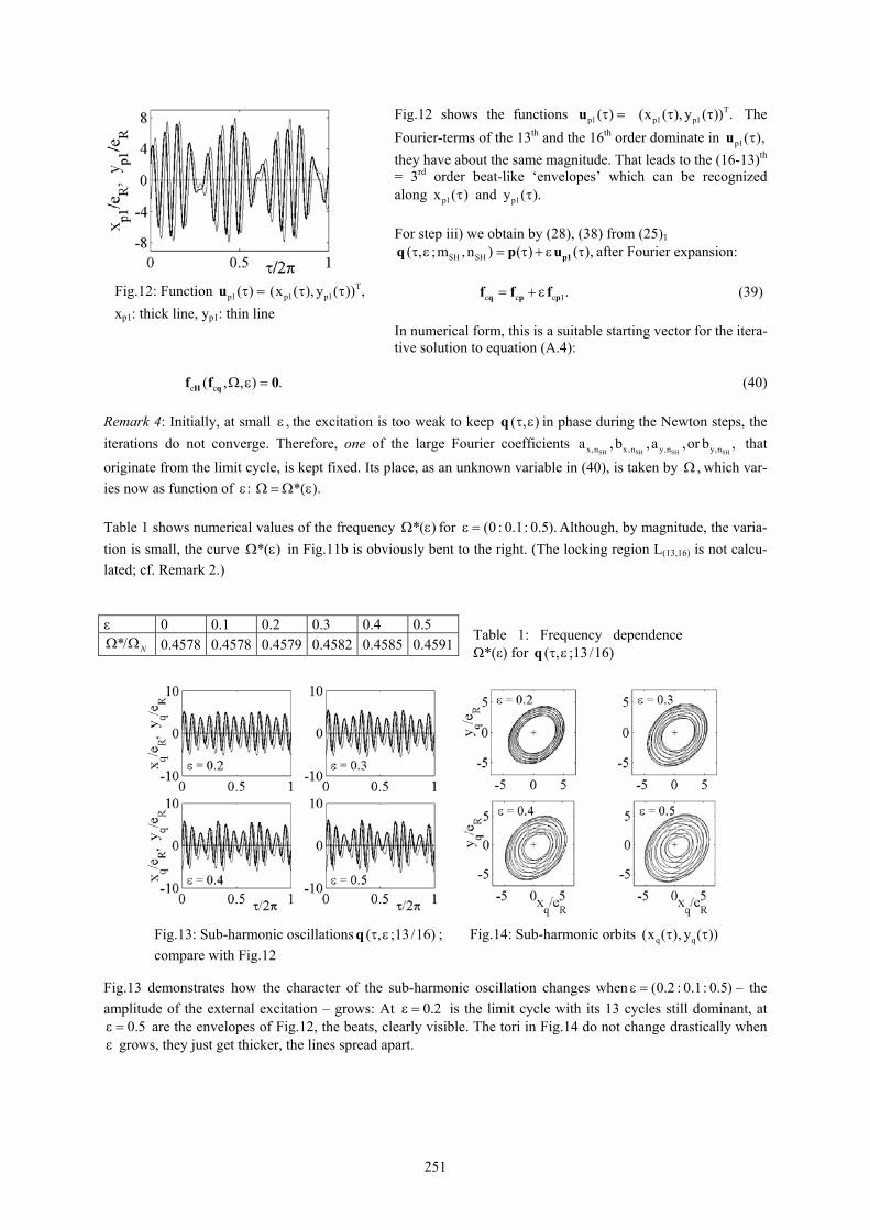
Fig.12 shows the functions p1( )τ = p1 p1(x ( ), y ( )τu The Fourier-terms of the 13
T) .τth and the 16th order dominate in p1( ),τu
they have about the same magnitude. That leads to the (16-13)th = 3rd order beat-like ‘envelopes’ which can be recognized
p1x ( )along τ and p1y ( ).τ For step iii) we obtain by (28), (38) from (25)1
SH SH( , ;m , n ) ( ) ( ),τ ε = τ + ε p1q p τu
1
after Fourier expansion: .c c c= + εq p pf f f (39) In numerical form, this is a suitable starting vector for the itera- tive solution to equation (A.4):
(40) c c( , , )Ω ε =H qf f 0. Remark 4: Initially, at small ε the excitation is too weak to keep , ( , )τ εq in phase during the Newton steps, the iterations do not converge. Therefore, one of the large Fourier coefficients that originate from the limit cycle, is kept fixed. Its place, as an unknown variable in (40), is taken by Ω which var-ies now as function of ε Ω
SH SH SH SHx,n x,n y,n y,na , b ,a ,or b,
,
).: *= Ω (ε Table 1 shows numerical values of the frequency *( )Ω ε for (0 : 0.1: 0.5).ε = Although, by magnitude, the varia-tion is small, the curve in Fig.11b is obviously bent to the right. (The locking region L*( )Ω ε (13,16) is not calcu-lated; cf. Remark 2.)
Table 1: Frequency dependence Ω*(ε) for ( , ;13 /16)τ εq
Fig.12: Function p1( )τ =u Tp1 p1(x ( ), y ( )) ,τ τ
xp1: thick line, yp1: thin line
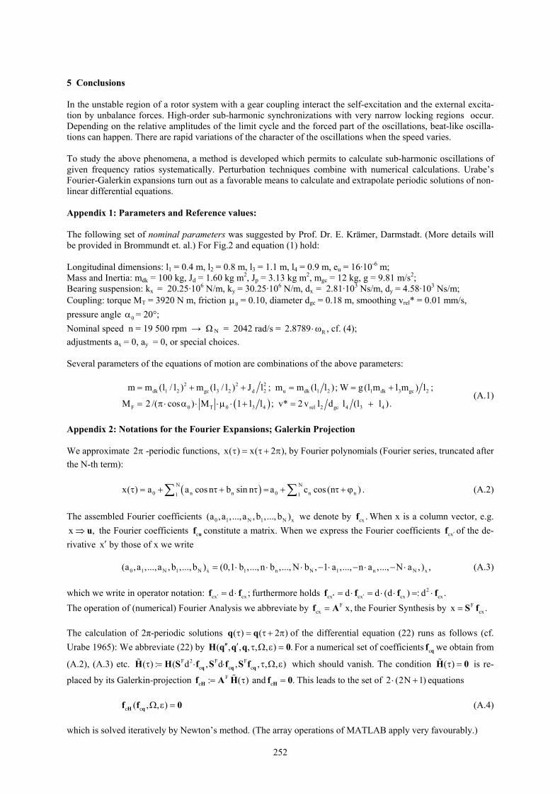
( , ;13 /16)τ εq q q(x ( ), y ( ))τ τ
Fig.14: Sub-harmonic orbits Fig.13: Sub-harmonic oscillations ; compare with Fig.12
Fig.13 demonstrates how the character of the sub-harmonic oscillation changes when ε = – the amplitude of the external excitation – grows: At
(0.2 : 0.1: 0.5)0.2ε = is the limit cycle with its 13 cycles still dominant, at
are the envelopes of Fig.12, the beats, clearly visible. The tori in Fig.14 do not change drastically when grows, they just get thicker, the lines spread apart.
0.5ε =ε
251
5 Conclusions In the unstable region of a rotor system with a gear coupling interact the self-excitation and the external excita-tion by unbalance forces. High-order sub-harmonic synchronizations with very narrow locking regions occur. Depending on the relative amplitudes of the limit cycle and the forced part of the oscillations, beat-like oscilla-tions can happen. There are rapid variations of the character of the oscillations when the speed varies. To study the above phenomena, a method is developed which permits to calculate sub-harmonic oscillations of given frequency ratios systematically. Perturbation techniques combine with numerical calculations. Urabe’s Fourier-Galerkin expansions turn out as a favorable means to calculate and extrapolate periodic solutions of non-linear differential equations. Appendix 1: Parameters and Reference values: The following set of nominal parameters was suggested by Prof. Dr. E. Krämer, Darmstadt. (More details will be provided in Brommundt et. al.) For Fig.2 and equation (1) hold: Longitudinal dimensions: l1 = 0.4 m, l2 = 0.8 m, l3 = 1.1 m, l4 = 0.9 m, eu = 16·10-6 m; Mass and Inertia: mdk = 100 kg, Jd = 1.60 kg m2, Jp = 3.13 kg m2, mgc = 12 kg, g = 9.81 m/s2; Bearing suspension: kx = 20.25·106 N/m, ky = 30.25·106 N/m, dx = 2.81·103 Ns/m, dy = 4.58·103 Ns/m; Coupling: torque MT = 3920 N m, friction 0µ = 0.10, diameter dgc = 0.18 m, smoothing vrel* = 0.01 mm/s, pressure angle α = 20°; 0
Nominal speed n = 19 500 rpm → Ω N = 2042 rad/s = R2.8789 ,⋅ω cf. (4); adjustments ax = 0, ay = 0, or special choices. Several parameters of the equations of motion are combinations of the above parameters:
( )
2 2 2dk 1 2 gc 3 2 d 2 u dk 1 2 1 dk 3 gc 2
F 0 T 0 3 4 rel 2 gc 4 3 4
m m (l / l ) m (l / l ) J l ; m m (l l ); W g(l m l m ) l ;
M 2 /( cos ) M 1 l l ; v* 2 v l d l (l l ).
= + + = = +
= π ⋅ α ⋅ ⋅µ ⋅ + = + (A.1)
Appendix 2: Notations for the Fourier Expansions; Galerkin Projection We approximate -periodic functions, 2π x( ) x( 2 ),τ = τ + π by Fourier polynomials (Fourier series, truncated after the N-th term): (A.2) ( )N N
0 n n 0 n1 1x( ) a a cos n b sin n a c cos (n ) .τ = + τ + τ = + τ + ϕ∑ ∑ n
,
;f .
The assembled Fourier coefficients we denote by f When x is a column vector, e.g.
the Fourier coefficients f constitute a matrix. When we express the Fourier coefficients of the de-rivative x by those of x we write
0 1 N 1 N x(a ,a ,...,a , b ,..., b ) cx .x ⇒ u cu cx′f
′ (A.3) 0 1 N 1 N x 1 n N 1 n N x(a ,a ,...,a , b ,..., b ) (0,1 b ,..., n b ,..., N b , 1 a ,..., n a ,..., N a , ) ,= ⋅ ⋅ ⋅ − ⋅ − ⋅ − ⋅&
which we write in operator notation: furthermore holds cx cxd′ = ⋅f 2
cx cx cx cxd d (d ) : d′′ ′= ⋅ = ⋅ ⋅ = ⋅f f f f The operation of (numerical) Fourier Analysis we abbreviate by f A the Fourier Synthesis by F
cx x,= Fcxx .= S f
The calculation of 2π-periodic solutions ( ) ( 2 )τ = τ + π
( , , , , , )′′ ′q q of the differential equation (22) runs as follows (cf.
Urabe 1965): We abbreviate (22) by .τ Ω ε =q q 0F
c c c, , , , )⋅ τ Ω εq q qf S fF ( )= τH% c
H qF, df S
:f A .
For a numerical set of coefficients f we obtain from
(A.2), (A.3) etc. which should vanish. The condition is re-
placed by its Galerkin-projection and
cq
F 2( ) : ( dτ = ⋅H H S%
cH
( )τ =H% 0
=Hf This leads to the set of 0 2 (2N 1)⋅ + equations (A.4) c c( , , )Ω ε =H qf f 0 which is solved iteratively by Newton’s method. (The array operations of MATLAB apply very favourably.)
252
References Brommundt, E.; Krämer, E.: Instability and self-excitation caused by a gear coupling in a simple rotor system. (2004) in preparation. Czerny, L.: Stabilitäts- und Schwingungsverhalten elastisch gelagerter Motoren mit Bogenzahnkupplung. VDI-
Berichte, Düsseldorf (1993), Vol. 1082, pp. 417 – 435. Deuflhard, P.; Bornemann, F.: Scientific Computing with Ordinary Differential Equations. Springer, New York
etc. (2002), 485 p. Deuflhard, P.; Hohmann, A.: Numerical Analysis in Modern Scientific Computing. 2nd Ed. Springer, New York
etc. (2003), 337 p. Farkas, M.: Periodic Motions. Springer-Verlag, New York etc. (1994), 577 p. Jordan, D. W.; Smith, P.: Nonlinear Ordinary Differential Equations; 2nd edit. Clarendon Press, Oxford (1987),
381 p. Ioos, G.; Joseph, D. D.: Elementary Stability and Bifurcation Theory. Springer-Verlag, New York etc. (1980),
286 p. Krämer, E.: Dynamics of Rotors and Foundations. Springer-Verlag, Berlin etc. (1993), 383 p. Ku, C.-P.R.; Walton Jr., J.F.; Lund, J.W.: A theoretical approach to determine angular stiffness and damping
coefficients of an axial spline coupling in high-speed rotating machinery. 14th Biennial Conference on Me-chanical Vibration and Noise (1993), pp. 249 – 256.
Morton, P.G.: Aspects of Coulomb damping in rotors supported on hydrodynamic bearings. Workshop on Rotor-
dynamic Instability Problems in High-Performance Turbomachinery, A&M University, College Station, Tex. (1982), Proceedings pp. 45 – 56.
Piotrowski, J.: Shaft Alignment Handbook; 2nd Edit., Marcel Dekker Inc, New York etc. (1995). Shiraki, K., Umemura, S.: On the vibrations of two-rotor system connected by gear couplings. Technical Review,
Mitsubishi Heavy Industries Ltd., Tokyo (Jan. 1970), pp. 22 – 33. Urabe, M.: Galerkin’s procedure for nonlinear periodic systems. Arch. Rational Mech. Anal. (1965), pp.120-152. Yamauchi, S.; Someya, T.: Self-excited vibration of gas-turbine rotor with gear coupling. 14th International
Congress on Combustion Engines (CIMAC), Helsinki (1981), pp. GT8-1 to GT8-28. __________________________________________________________________________________________ Address: Prof. em. Dr. Eberhard Brommundt. Institut für Dynamik und Schwingungen, Technische Universität Braunschweig, PF 3329, D-38023 Braunschweig (Germany). e-mail: [email protected]


![Modes shape and harmonic analysis of different structures ... · the fuselage has an influence on the rotor hub [18-19]. The models of the associated rotor-fuselage are required,](https://static.documents.pub/doc/80x56/5e0e83874f7ada76a21866b4/modes-shape-and-harmonic-analysis-of-different-structures-the-fuselage-has-an.jpg)


