High spatial resolution burn severity mapping of the NewJersey Pine Barrens with WorldView-3 near-infrared andshortwave infrared imageryTimothy A. Warner a, Nicholas S. Skowronski b and Michael R. Gallagher c
aDepartment of Geology and Geography, West Virginia University, Morgantown, WV, USA; bUSDA ForestService, Northern Research Station, Morgantown, WV, USA; cUSDA Forest Service, Northern ResearchStation, New Lisbon, NJ, USA
ABSTRACTThe WorldView-3 (WV-3) sensor, launched in 2014, is the first high-spatial resolution scanner to acquire imagery in the shortwave infra-red (SWIR). A spectral ratio of the SWIR combined with the near-infrared (NIR) can potentially provide an effective differentiation ofwildfire burn severity. Previous high spatial resolution sensors werelimited to data from the visible and NIR formapping burn severity, forexample using the normalized difference vegetation index (NDVI).Drawing on a study site in the Pine Barrens of New Jersey, USA, weinvestigate optimal processing methods for analysing WV-3 data,with a focus on the pre-fire minus post-fire differenced normalizedburn ratio (dNBR). Although the imagery, originally acquired with a3.7 m instantaneous field of view, was aggregated to 7.5 m pixels byDigitalGlobe due to current licensing constraints, a slight additionalsmoothingof the datawas nevertheless found tohelp reduce noise inthe multi-temporal dNBR imagery. The highest coefficient of deter-mination (R2) of the regressions of dNBR with the field-based compo-site burn index was obtained with a dNBR ratio produced with theNIR1 and SWIR6 bands. Only a very small increase in R2 was foundwhendNBRwas calculated using the average of NIR1 andNIR2 for theNIR bands, and SWIR5 to SWIR8 for the SWIR bands. dNBR calculatedusing SWIR1 as the NIR band produced notably lower R2 values thanwhen either NIR1 or NIR2 were used. Differenced NDVI data wasfound to produce models with a much lower R2 than dNBR, empha-sizing the importance of the shortwave infrared region formonitoringfire severity. High spatial resolution dNBR data fromWV-3 can poten-tially provide valuable information on finer details regarding burnseverity patterns than can be obtained from Landsat 30 m data.
ARTICLE HISTORYReceived 24 August 2016Accepted 20 November2016
1. Introduction
The launch of DigitalGlobe’s WorldView-3 (WV-3) sensor on 13 August 2014, openednew opportunities in satellite-borne mapping of wildland fire burn severity (Keeley 2009)using short wave infrared (SWIR; 1.4–2.5 µm) data at a finer spatial resolution than hasbeen previously possible. A long history of research suggests that mapping of forest fire
CONTACT Timothy A. Warner [email protected] Department of Geology and Geography, WestVirginia University, P O Box 6300, Morgantown, WV 26506-6300, USA
INTERNATIONAL JOURNAL OF REMOTE SENSING, 2017VOL. 38, NO. 2, 598–616http://dx.doi.org/10.1080/01431161.2016.1268739
burn severity is generally most effective with a spectral ratio that combines near-infrared(NIR; 0.7–1.4 µm) and SWIR (e.g. Garcia and Caselles 1991; Key and Benson 1999; Key2006; Parks, Dillon, and Miller 2014). This ratio is especially successful if applied toimagery acquired immediately before and after the burn (Key and Benson 2006). TheWV-3 sensor acquires eight visible (0.4–0.7 µm) and NIR bands, and unlike any previoushigh-spatial resolution sensor, can in addition acquire a further eight longer wavelengthbands in the NIR and SWIR region (Table 1) (Kruse, Baugh, and Perry 2015; DigitalGlobe2016). The eight visible and NIR WV-3 bands have a 1.2 m instantaneous field of view(IFOV), whereas the eight NIR and SWIR bands have an IFOV of 3.7 m, though currentlythis latter group of bands is degraded for the general public to 7.5 m pixels inaccordance with licensing restrictions. Thus, WV-3 is significant both for its finer spatialresolution and its increased spectral resolution.
The importance of having access to high resolution SWIR data for mapping burn severityis demonstrated by Figure 1, which shows both the WV-3 bands and spectral reflectance
Table 1. WorldView-3 band centre wavelengths.Band name Band number Centre wavelength (nm) Spectral regiona
See also Figure 1.a For the purpose of this article, we define the visible as 0.4–0.7 µm, NIR 0.7–1.4 µm, and SWIR 1.4–2.5 µm.
Figure 1. WorldView-3 band spectral response functions (left axis) by band (see numbers at the topof the graph) (DigitalGlobe 2016) and comparison to field spectral reflectance measurements of keycover types from the Penn State Forest.
INTERNATIONAL JOURNAL OF REMOTE SENSING 599
field measurements of various land cover materials relevant for forest fire mapping.Compared to green pine needles, scorched pine needles show effects across the entirespectrum: increased blue and red, decreased NIR, and increased SWIR reflectance. Burntplant matter, including litter and bark, which is black to the naked eye, has a generally lowand featureless spectrum, although it does show a characteristic rise at longer wavelengths,resulting in characteristically SWIR reflectance that can be higher than that of greenvegetation. The combination of reduced NIR and increased SWIR is, therefore, generallyvery effective for mapping burn severity (Key and Benson 1999, 2006).
Prior burn severity mapping has beenmostly carried out using Landsat Thematic Mapper(TM), Enhanced Thematic Mapper Plus (ETM+), andOperational Line Imager (OLI) sensors, allwith 30 m IFOV in the SWIR region (Garcia and Caselles 1991; Key and Benson 2006). Othersatellite-borne sensors with SWIR bands that have been used for fire mapping include theModerate Resolution Imaging Spectroradiometer (MODIS) with 500 m pixels (Chen, Sheng,and Liu 2015), the Advanced Spaceborne Thermal Emission and Reflection Radiometer(ASTER), with 30 m SWIR pixels (Holden et al. 2010), Satellite Pour l’Observation de laTerre (SPOT) 4 and 5 sensors with 20 m SWIR pixels (Polychronaki and Gitas 2012) and theEuropean Space Agency’s Multispectral Imager (MSI) on the Sentinel-2A satellite, also with20 m pixels (Fernández-Manso, Fernández-Manso, and Quintano 2016). Thus, even with adegraded spatial resolution of 7.5 m, WV-3 data represents a substantial increase inpotential detail over previously available satellite-borne sensors.
High spatial resolution mapping of burn severity from space-borne sensors could beparticularly valuable for improved understanding of fire behaviour and for ecologicalrestoration work, particularly for studying smaller fires in areas regarded as having highecological value. For example, high resolution mapping could be useful for prescribedfires for forests close to inhabited areas, where the fires, though small, may be con-tentious and difficult to implement (Clark, Skowronski, and Gallagher 2015; Skowronskiet al. 2015). Prior high spatial resolution sensors, such Airbus Defense & Space’s Pléiadesand DigitalGlobe’s WorldView-2 (WV-2) sensors were limited to four, or at most eight,spectral bands, but crucially the bands were entirely within the visible to NIR range,typically no further than about 1.0 µm. Prior high spatial resolution sensors were there-fore limited to mapping burn severity using visible and NIR wavelengths, for exampleusing ratios such as the normalized difference vegetation index (NDVI; Rouse et al. 1974).
With its multiple high-spatial resolution SWIR bands, WV-3, therefore, offers sig-nificant opportunities for mapping burn severity. However, this new sensor also raisesmany questions that need to be addressed prior to routine use of the data. Inparticular, the choice of specific bands to use in developing the burn ratio is ofsome importance given that there are seven WV-3 SWIR bands and three NIR bandsto select from. A related question is whether it is better to aggregate the SWIR bands,potentially to increase the signal to noise ratio, an approach that could be useful forwinter acquisitions, when solar illumination is weak (Warner, Nellis, and Foody 2009).Furthermore, the eight visible and NIR bands are not necessarily provided as apackage with the eight longer wavelength bands, raising another important issueas to whether effective burn severity mapping can be achieved using only the lattergroup of bands alone, especially since this group includes a NIR band at 1.2 μm. If aresearcher only needs to purchase the eight longer wavelengths bands, this couldresult in considerable cost savings. In addition to addressing these methodological
600 T. A. WARNER ET AL.
questions, we also ask whether, at least within the context of our study site, burnseverity products generated at 7.5 m provide potentially more useful informationthan what can be discerned at 30 m, for example in a typical Landsat product. Finally,we also compare ratio products that use the SWIR band to NDVI, in order to confirmthat the SWIR data really is useful for studying forest fire burn severity in our studyarea.
2. Background
The normalized burn ratio (NBR) is defined (Key and Benson 2006) as
NBR ¼ ρNIR � ρSWIR
ρNIR þ ρSWIR; (1)
where ρ is reflectance, and the subscripts NIR or SWIR describe the spectral regions.Generally, the 2.0–2.4 µm (e.g. Landsat TM band 7) atmospheric window is regarded as abetter choice for the SWIR band than the 1.5–1.8 µm (e.g. TM band 5) window (VanWagtendonk, Root, and Key 2004; Veraverbeke, Harris, and Hook 2011). There is a longhistory of the use of using a differenced NBR product (dNBR) to map burn severity (Keyand Benson 2006; Escuin, Navarro, and Fernandez 2008):
dNBR ¼ NBRð Þpre�fire � NBRð Þpost�fire; (2)
where the subscripts pre-fire and post-fire refer to the timing of the acquisition of theimagery. In this article, we will apply the term dNBR to any differenced ratio images,employing NIR and SWIR bands, as defined earlier.
The dNBR measure has been found to be highly effective for mapping burn severity,particularly in forested environments (Van Wagtendonk, Root, And Key 2004; Key andBenson 2006). Nevertheless, variations on dNBR have been proposed to address short-comings with the ratio. For example, a relative version of the dNBR can be used if thereare large differences in the pre-fire canopy density (Miller and Thode 2007; Parks, Dillon,and Miller 2014). Another variation is to include spectral emissivity in the ratio(Fernández-Manso and Quintano 2015). For comparisons between multiple fires, anoffset to the dNBR is sometimes applied to normalize the values so that they arecomparable between fires (e.g. Miller et al. 2009). Entirely different approaches, suchas machine-learning, have also been proposed where high spectral resolution data areavailable (Hultquist, Chen, and Zhao 2014).
Despite its success in forested environments, dNBR has been found to be lesseffective in other environments, such as grasslands (Lu, He, and Tong 2016). Similarly,Roy, Boschetti, and Trigg (2006) found that the ratio is not optimal for mapping fire insavannah vegetation.
Prior to the launch of WorldView-3, high spatial resolution sensors were generallylimited to visible and NIR wavelengths. Typically, studies using such data have employedNDVI (Rouse et al. 1974) or similar vegetation indices. NDVI is defined as
NDVI ¼ ρNIR � ρRedρNIR þ ρRed
; (3)
INTERNATIONAL JOURNAL OF REMOTE SENSING 601
where, as before, ρ is reflectance, and the subscripts NIR or Red describe the spectralregions. A differenced NDVI index (dNDVI) can also be generated, as with dNBR, bydifferencing pre-fire and post-fire images. Many variations of NDVI and similar indiceshave been proposed to improve the effectiveness of using NIR and visible bands formapping burn severity (Chuvieco, Martin, and Palacios 2002; Boelman, Rocha, andShaver 2011).
Although NDVI is very reliable for measuring the presence of vegetation, the effect ofburning can be confused with other losses of vegetation, and using NDVI to monitorburn severity is less effective if imagery is acquired when the vegetation has senesced.Many studies that have evaluated the use of high resolution dNDVI products have foundthem less effective than Landsat dNBR products (e.g. Escuin, Navarro, and Fernandez2008). However, Holden et al. (2010) found that a differenced enhanced vegetationindex (a modified version of NDVI) derived from QuickBird data produced a highercoefficient of determination (R2) for regression models of field measures of burn severitythan was achieved with Landsat TM dNBR data for a ponderosa pine study area in NewMexico, USA. Furthermore, Wu et al. (2015), in a study of ponderosa, pinyon, juniper, andoak forests in Arizona, USA, found that Landsat-derived dNDVI resulted in a higher R2
than Landsat dNBR, or indeed than indices from WV-2 high-spatial resolution data, whenregressed against burn severity.
In an important study using a radiative transfer model, Chuvieco et al. (2006) showedthat a spectral ratio of NIR and red is potentially the most effective combination formapping recent fires, where charcoal dominates the spectral signal. In contrast, ratiosusing NIR and SWIR provided the highest potential accuracy for a wider range of fires,both recent and older, and where soil, charcoal, and both green and brown leaves arepresent.
3. Study area
The study area is the Penn State Forest (Figure 2), in the New Jersey Pinelands NationalReserve (PNR). Forests in this study area are primarily: ‘pine–oak forests’, consisting ofpitch pine with mixed oaks in the overstory; ‘pine–scrub oak forests’, dominated bypitch pine with understory scrub oaks (Q. ilicifolia Wang. and Q. marlandica Muench.)in the understory (McCormick and Jones 1973; Lathrop and Kaplan 2004); or ‘pineplains’ which have a similar species assemblage to ‘pine-scrub oak forest’ but arecharacterized by very short statured stems (<2 m). Ericaceous shrubs are the majorunderstory component of all of these forest types, primarily huckleberry (Gaylussaciabacata (Wang.) K. Koch, G. frondosa (L.) Torr. & A. Gray ex Torr.) and blueberry(Vaccinium spp.). The soils are sandy and acidic (La Puma, Lathrop, and Keuler 2013),and the topography is generally flat.
This landscape of the PNR is characterized by a high frequency and intensity ofwildfires relative to other forest ecosystems in the northeastern USA. The study areahas had a history of periodic wildfire events, with the largest occurring in 1948 and 1982(La Puma, Lathrop, and Keuler 2013). These fires both burned a significant portion ofPenn State Forest and there have been several smaller fires as well, most prior to 1982.Prescribed fire has been intermittently introduced to small, peripheral, stands within thestudy area with little effect on canopy fuel loading (H. Somes, New Jersey Forest Fire
602 T. A. WARNER ET AL.
Service Division Fire Warden (retired), personal communication, 18 August 2016). For thisstudy, nearly the entirety of Penn State Forest was burned on several days between 29February and 18 March 2016. These burns were conducted under a wide range ofmeteorological conditions and fuel moistures with ignition patterns varying from back-ing, heading, and plastic sphere aerial ignition (many interior spot fires). An additional150 ha within the study area burned in a wildfire on 10 March 2016.
4. Methods
4.1. Field methods
A total of 156 random samples were selected over the study site (Figure 2(b)).Although prior studies have selected samples using a stratified approach based ondNBR values (Key and Benson 2006) or site conditions (Kasischke et al. 2008), wechose a purely random approach combined with a relatively large number of samplesto provide the simplest, direct, and most reliable estimate of the accuracy of theremotely sensed fire severity map. Our site is characterized by large areas of relativelylow, moderate and intense burn intensities, making a purely random approachfeasible. On the other hand, in an area without much variation in burn severity, astratified approach might be necessary. Furthermore, we did not bias our selection to
Figure 2. WorldView-3 false colour imagery (bands 16, 7, 5 as RGB) of Penn State Forest, New JerseyPine Barrens. (a) Pre-burn image, acquired on 8 December 2015. (b) Post-burn image, acquired on 13April 2016. Locations of field samples and associated Total CBI class are also indicated.
INTERNATIONAL JOURNAL OF REMOTE SENSING 603
areas of relatively homogeneous burn severity, as is recommended by Key andBenson (2006). The disadvantage of our approach is that error in the georeferencingof the image or field sample locations will potentially translate into increased appar-ent spectral burn severity error, and result in an unnecessarily conservative estimateof overall accuracy. Nevertheless, we argue that it is highly possible that burnseverity-estimation error is more common in mixed pixels, and therefore a samplingapproach that systematically avoids areas of potential error would seem to be likelyto generate an overly optimistic estimate of accuracy. For all these reasons, we arguethat the approach we adopted produces the highest possible confidence in theaccuracy estimates, and that, if anything, our approach is conservative.
The field measurements were made between 12 March and 6 April 2016, immediatelyafter areas were burnt. Field procedures for estimating the composite burn index (CBI)employed the Key and Benson (2006) field data sheet. One key difference, however, isthat we modified the diameter of the field plot from the recommended 30 m, to 15 m, inorder to accommodate the finer scale of the WV-3 data compared to Landsat.
The CBI encompasses estimates of burn severity for five main strata of the vegetation:substrate, including litter and duff; herbs, low shrubs, and trees less than 1 m tall; tallshrubs and trees 1–5 m; intermediate trees, including sub-canopy and pole-sized trees;and big trees, including canopy, dominant and co-dominant trees (Key and Benson2006). Within each stratum, burn-severity for each component within that stratum isestimated on a 0.0–3.0 scale. By averaging the burn severity values within each stratum,an index is obtained for that stratum. The values for the strata are then averaged toproduce integrated understory, overstory, and overall burn indices.
Field spectra, shown in Figure 1, were collected on 12 March 2016, using a FieldSpec-2, portable field spectrometer (ASD Inc., Boulder CO, USA). A portable lamp provided byASD was used for illumination, and spectra were normalized to a Labsphere (NorthSutton, NH, USA) Spectralon barium sulphate reflectance standard (Asmaryan et al.2013).
4.2. Image acquisition, pre-processing and analysis
A pre-fire image, including all 16 visible, NIR and SWIR bands, was acquired on 8December 2015. (For convenience, we will refer to the bands by the numbers from1–16, please refer to Table 1 for the associated wavelengths and the names given to thebands by DigitalGlobe.) As a winter scene, the sun elevation was 26.8°, and the mean off-nadir viewing angle was 6.3°. A post-fire image was acquired on 13 April 2016, with anotably higher sun elevation of 57.9° and a mean off-nadir viewing angle of 12.3°. The 4month interval between the pre- and post-fire burn images is less than optimal in thatany phenological changes in that time will likely reduce the accuracy of burn severitymapping. However, the acquisitions were timed to be after leaf senescence in the fall,and prior leaf expansion in the spring, and therefore plants were dormant in bothimages. In any case, given the challenges of acquiring snow-free and cloud-free imagesin the winter and early spring in the eastern United States, this period of time betweenacquisitions was the best we could achieve, and may be representative of what anoperational fire monitoring programme would have to accommodate.
604 T. A. WARNER ET AL.
The images were imported in to ENVI 5.3 (Exelis Visual Information Solutions, Boulder,CO, USA). The images were converted into radiance, and then surface reflectance usingthe Fast Line-of-sight Atmospheric Analysis of Hypercubes (FLAASH) module within ENVI(Cooley et al. 2002). FLAASH is built around the MODTRAN radiative transfer model, andis able to deal with the non-nadir viewing effects.
The reflectance images were then imported into ERDAS Imagine 2015 (HexagonGeospatial Inc., Norcross, GA, USA), and co-registered using the Imagine Autosyncfeature, which matches images using automatically generated tie-points. The imageswere then used to generate a variety of WV-3 dNBR ratio products, using bands 7, 8, or 9as the NIR band, and one of the bands between 10 and 16 as the SWIR band (see Table 1for the band designations, see Table 2 for the ratio combinations developed). In addi-tion, two NDVI products (with band 6 for red and 7 or 8 as NIR) were generated. Broad-band NBIR ratio products were developed by averaging values across multiple NIR andSWIR bands, prior to calculating the ratios.
Table 2. Summary statistics for various dNBR products for describing composite burn index (CBI)values.
a See Table 1 and Figure 1 for key to band numbers.The ‘:’ symbol is used to indicate the average of a range of bands, e.g. ‘7:8’ means bands the average of bands 7 and 8.Minimum and maximum R2 values for single band ratios are shown, respectively, underlined and in bold. Themaximum values R2 for broad band ratios (using averages of multiple bands) are shown in bold italics.
INTERNATIONAL JOURNAL OF REMOTE SENSING 605
Despite the Autosync co-registration, small differences between the December andApril images could still be seen, when the images were overlaid. These appear to be realdifferences, reflecting differences in the shadowing and parallax effects from the differ-ent view angles and the varying tree heights. We, therefore, also developed a smoothedproduct, in addition to the raw dNBR images. The smoothed image was produced usinga low-pass filter, where the values in a 3 × 3 pixel kernel follow a Gaussian curve, with aone-standard deviation (σ) of 0.85 (Brandtberg et al. 2003). We also used pixel aggrega-tion to generate a dNBR product with a 30 m pixel size, to simulate the spatial resolutionof Landsat imagery. We chose this approach of simulating a coarser resolution imagery,rather than using real Landsat data, in order to produce comparison images that onlydiffered in spatial resolution.
For visualization of the images we followed a standardized procedure to develop aconsistent mapping from dNBR to image colour. A linear stretch on a scale of 0–255 wasapplied to the dNBR values between a dNBR of 0 and the 99.95 percentile; valuesoutside that range were saturated at 0 and 255, respectively. A standard ERDASImagine pseudo colour palette was then applied to the scaled values for all valuesabove an empirically chosen threshold of 85; values below that value were shown ingrey scale.
Two procedures were investigated for relating the dNBR values from the WV-3imagery and the field samples. The key issues were that the centre of the field sampleswere not necessarily in the centre of a pixel and the field sampling was done over a15 m diameter area, compared to the 7.5 m size of the pixels. The first method used thespectral values of the single pixel of Gaussian smoothed imagery, as discussed earlier, inwhich the point fell. The second approach used an area-weighted approach applied tothe original, unsmoothed data. In this approach, a 15 m diameter circle was drawnaround the centre of the field sample location. The proportion of the circle in each of theunderlying pixels was then multiplied by the associated pixel reflectance, and the valuessummed. The two approaches produced almost identical results when the spectralvalues were regressed against CBI values. Although the low pass filter approach ismuch easier to implement, we chose the area weighted approach as being conceptuallymore appealing.
The various differenced WV-3 ratio data were regressed against the CBI data. Visualinspection indicated that the variables were non-linearly related, therefore, an exponen-tial model was chosen.
5. Results and discussion
5.1. Quantitative results
Figure 3(a) summarises the average reflectance of the field sites, as measured in the 8December 2015 WV-3 imagery, prior to the burn. The spectra are grouped based on theseverity of burn, as estimated in the field, after the fire. The graph indicates the field siteswere on average mostly similar, at least spectrally. However, the pixels that wereclassified as having the highest burn severity (i.e. CBI values of 2.5–3.0) had noticeablyhigher average SWIR reflectance prior to the burn, possibly indicating drier conditions inthose areas (Van Leeeuwen 2009).
606 T. A. WARNER ET AL.
Figure 3. Average reflectance from WV-3 imagery for different classes of CBI. The numbers refer tothe WV-3 band numbers (see Table 1). (a) Spectral reflectance from WV-3 imagery of 8 December2016 (pre-fire). (b) Spectral reflectance from WV-3 imagery of 13 April 2016 (post-fire). (c) Change inspectral reflectance, from 8 December 2015 (pre-fire) to 13 April 2016 (positive values indicatereflectance increase).
INTERNATIONAL JOURNAL OF REMOTE SENSING 607
Figure 3(b) shows the post-fire WV-3 reflectance spectra for the sample plots, alsogrouped by CBI value. Figure 3(c) shows the difference in reflectance between beforeand after the fire. Ideally, Figure 3(c) should show no change at all for the CBI class of 0.0,but in the SWIR bands in particular a reflectance change of approximately 0.04 is apparent.This could indicate real phenological changes in the 4 months between the two acquisi-tions as well noise, for example, due to uncertainties in the conversion to reflectance.
The results shown in Figure 3 are broadly consistent with the field spectra of Figure 1. Inparticular, the effect of fire is small and inconsistent in the visible, especially the red (band5; 0.66 µm), where, with increasing CBI value, red reflectance first increases, most likely dueto scorching of needles, but then decreases, as charred vegetation dominates. In contrast,in the NIR, particularly bands 7 (0.83 µm) and 8 (0.95 µm), there is a generally large andconsistent decline in reflectance as CBI increases. For the NIR band 9 (1.2 µm) the changein reflectance is smaller than in the other NIR bands, and there is some inconsistency.For example, CBI class 0.5–1.0 is associated with a lower average reflectance than pixelswith a CBI class of 1.0–1.5. The SWIR region also generally is associated with a large andconsistent increase in reflectance as the CBI class increases, with the change greater in thelonger 2.1–2.3 µm region (bands 13–16) than the shorter SWIR wavelengths of 1.6–1.7 µm(bands 10–12), particularly for the higher CBI value classes (i.e. more intensely burnt areas).
In summary, Figure 3 suggests that for the study area, NDVI is unlikely to be a usefulmeasure of burn severity, particularly due to the relatively large and inconsistent changein red wavelengths. Furthermore, the NIR bands, 7 and 8 are likely to provide a moreuseful estimate of burn severity than 9. Of the SWIR bands (bands 10–16), the longerwavelength bands 13–16 appear to be the most useful.
Examples of the exponential regression models are shown in Figure 4; the completeresults are listed in Table 2. Using CBI as the independent variable, and the differencedindividual band dNBR data as the dependent variable, the exponential regressionmodels resulted in coefficient of determination (R2) values that vary from a low of0.696 (using bands 7 and 11 as the NIR and SWIR bands, respectively) to a high of0.841 (using bands 7 and 14). Notably, differencing using NDVI, the only option availablein prior civilian high-resolution sensors, results in a much lower R2 values of 0.647 and0.693. These low R2 values are consistent with the prediction of likely inconsistent NDVIchanges with varying burn severity, as indicated by Figure 3.
Integrating adjacent NIR and/or adjacent SWIR bands was generally beneficial, so thatoverall the highest R2 value of 0.844 was obtained where the NIR bands was band 7 alone orintegrated with 8, and the SWIR bands was the average of bands 13–16. However, thedifference in R2 values between the single band and the broad band ratios is very small,only a matter of 0.004. The combination of bands designed to be similar to the spectralresponse of Landsat 8 OLI (band 7 for the NIR, and the average of bands 13–15 for the SWIR)results in a regression model with an R2 very similar to the values for the data generated withthe other broad-band differenced ratios.
The CBI is a summary measure based on both overstory and understory components.When the regression model is developed using the overstory component only, there is asmall, but consistent increase in the R2 values. The regression models built entirely on the CBIunderstory component have much greater scatter (Figures 4 (e) and (f)), and consequently alower R2, typically around 0.5 (Table 2). These results are not surprising; the understory isgenerally partially or totally obscured from the satellite view by the overstory. The overstory
608 T. A. WARNER ET AL.
clearly dominates in the satellite signal. One potential way of addressing this issue in futureresearch would be to employ the GeoCBI of de Santis and Chuvieco (2009), which adjusts theestimate of CBI by fraction of cover of each layer. Such an approachmight possibly result in animproved correlation between field and image estimates of burn severity.
5.2. Visual analysis
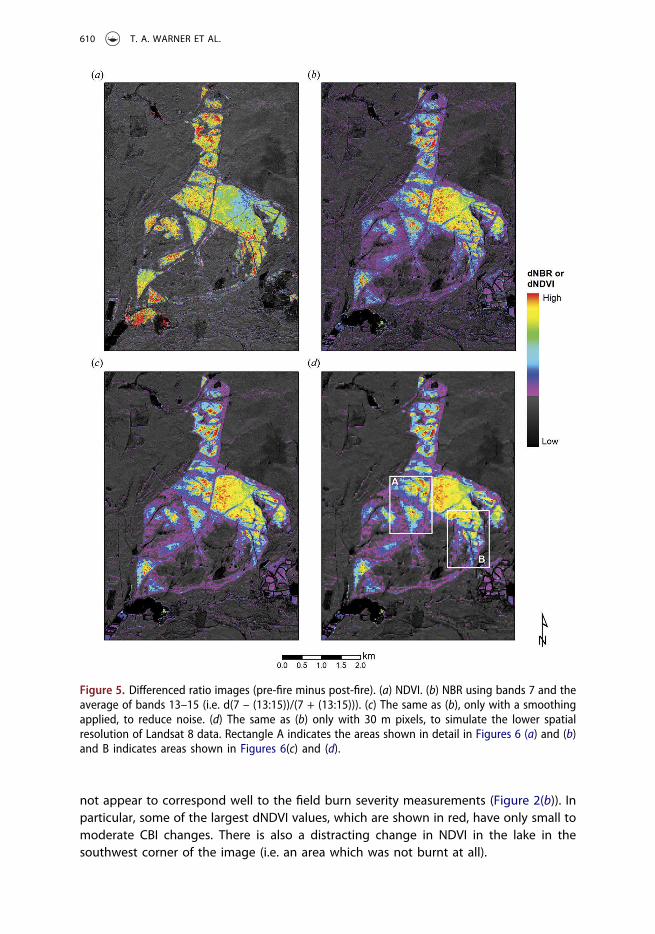
Figure 5(a) shows an example dNDVI image, and Figure 5(b) an example dNBR image.The dNDVI patterns are notably different from that of the nNBR image, and visually do
Figure 4. Scatterplots of CBI value versus example dNBR image ratios. Note that ‘d’ in the ratio isused to imply the before and after fires are differenced. (a), (c), and (e): Single band ratio usingbands 7 and 14. (b), (d), and (f): Ratio using band 7 and integrated values from bands 12 to 14.(RMSE stands for root mean square error.)
INTERNATIONAL JOURNAL OF REMOTE SENSING 609
not appear to correspond well to the field burn severity measurements (Figure 2(b)). Inparticular, some of the largest dNDVI values, which are shown in red, have only small tomoderate CBI changes. There is also a distracting change in NDVI in the lake in thesouthwest corner of the image (i.e. an area which was not burnt at all).
Figure 5. Differenced ratio images (pre-fire minus post-fire). (a) NDVI. (b) NBR using bands 7 and theaverage of bands 13–15 (i.e. d(7 – (13:15))/(7 + (13:15))). (c) The same as (b), only with a smoothingapplied, to reduce noise. (d) The same as (b) only with 30 m pixels, to simulate the lower spatialresolution of Landsat 8 data. Rectangle A indicates the areas shown in detail in Figures 6 (a) and (b)and B indicates areas shown in Figures 6(c) and (d).
610 T. A. WARNER ET AL.
The differenced image at the original resolution (Figure 5(b)) has small, isolated areasof moderate values scattered throughout the unburnt area, which could be confusedwith a low severity burn. The Gaussian low pass filter suppresses much of this noise,whilst preserving the majority of the spatial patterns (Figure 5(c)). The fact that smooth-ing is apparently necessary, even though the WV-3 SWIR data are provided at 7.5 m
Figure 6. Detail of dNBR images. (a) and (c) show the ratio images with 7.5 m pixels. (b) and (d)illustrate the level of detail with 30 m pixels, equivalent to the spatial resolution of Landsat 8. (SeeFigure 5 for location information.)
INTERNATIONAL JOURNAL OF REMOTE SENSING 611
resolution instead of the original 3.7 m IFOV, suggests that, at least for fire applications,the degradation of resolution to conform with the US licensing requirements may notmatter greatly. Indeed, if at a future stage higher spatial resolution SWIR data is released,it is likely that users will need to apply an even greater smoothing prior to calculatingthe dNBR.
Other areas of moderate dNBR values that incorrectly indicate a low severity burn canbe found in the southeast corner of Figure 5(c), where small, generally geometric regionsof dominantly purple colour can be seen. Reference to Figure 2 indicates these areas areassociated with changes in the water status in cranberry bogs, most likely due todrawing down of water levels in preparation for spring bud break.
Finally, we consider whether WV-3, with 7.5 m pixels, provides useful additionalspatial information for monitoring wildland or prescribed fires. This is explored in thezoomed areas in Figure 5, shown in Figure 6. Figures 6(a) and (c) show the 7.5 msmoothed data, and Figures 6(b) and (d) the same areas, except with 30 m pixels. The7.5 m data clearly shows the patterns in both high severity burns as well as the lowerseverity burn areas are much clearer. For example, in Figure 6(a), the fire spread patternsin the centre of the triangular field can be discerned with the 7.5 m pixels, but not 30 mpixels. Similarly, south of diagonal road, the 7.5 m data clearly shows two separate armsof high severity burn areas, which then coalesce. In the 30 m data, only a single highseverity pixel is indicated. The 7.5 m data also shows notably more detail of burnpatterns in low severity areas, sometimes in linear patterns possibly relating to differ-ences in moisture or species composition, for example along drainage lines. This level ofdetail would be beneficial to studies focused on linking fine-scale environmental driversof fire behaviour to the resulting severity.
6. Conclusions
The results of this study broadly indicate the value of WV-3 high spatial resolution(7.5 m) SWIR bands for monitoring burn severity. The high R2 value (up to 0.844) forthe regression of field-measured CBI values and the ratioed WV-3 data incorporating theSWIR bands provides strong empirical support that the fine detail of patterns observedin the imagery, such as in Figure 6, provides meaningful information about fine scalevariations in burn severity. The NDVI-based mapping of burn severity was not a suitablealternative for this site.
The WV-3 SWIR data have an IFOV of 3.7 m, but were degraded to 7.5 m in terms ofthe DigitalGlobe licensing agreement. At some future date, the higher resolution datamay be released. Our experience, in which a light smoothing using a Gaussian filter wasimportant for reducing noise in the differenced ratio product, suggests that resolutionfiner than 7.5 m may open new challenges. At the very least, a more intense smoothingthan that used in our work may be needed.
The eight bands acquired as part of the WV-3 SWIR package include-band 9 in theNIR, at 1.2 µm. It would, therefore, seem attractive to use this band as the NIR band incalculating the burn ratio instead of bands 7 or 8, from the VNIR bands, which poten-tially require a separate purchase. However, the best R2 obtained with band 9 was 0.795,0.049 lower than the 0.844 maximum obtained using band 7, or 7 and 8 combined. Thus,
612 T. A. WARNER ET AL.
at least for this study site, there appears to be a distinct benefit in obtaining all 16 bandsand not just the eight so-called SWIR bands.
Our recommendation is to use band 7 for the NIR band and 14 for the SWIR band, inthe calculating dNBR. These two bands had the highest overall coefficient of determina-tion using single bands, with an R2 of 0.841. This was very close to the best R2 whenband 7, or 7 and 8 combined, were used as the NIR band and bands 13–16 combined asthe SWIR band. In addition, the simulated broad-band Landsat OLI ratio resulted in avery similar R2. Together, these results suggest that for burn severity mapping, thenarrow bands of WV-3 produce potentially similar results to those of sensors withbroader bands, such as Landsat 8 OLI or similar sensors. Thus, from the perspective ofthe user, it is probably simpler to use single bands, rather than to combine them.However, an important caveat is that, in our study, the topography was essentiallyflat. In rugged terrain, we recommend evaluating whether combining WV-3 bands 7and 8 for the NIR band and 13–16 for the SWIR band improves the mapping of burnseverity on poorly illuminated slopes (Veraverbeke et al. 2010).
WV-3 is a commercial satellite, and therefore purchasing the data require consider-able financial outlay, unlike Landsat. This will of course constrain the use of data.Nevertheless, for fires of relatively small spatial extent, but of high value for ecologicalresearch or restoration or even perhaps for monitoring fires that encroach on structuresin urban areas, the high resolution of the WV-3 data could be very valuable. High spatialresolution burn severity could be useful for relating to subsequent regrowth in leaf areaindex (Rachels et al. 2016), or for relating to other sensors, such as lidar (Skowronski et al.2015), in order to study the linkages between fuel structure and loading to fire severityin ways that are not possible at a coarser resolution. This level of detail potentiallyprovides important differentiation of fire spread patterns, and information that could beused for studying fire recovery.
An added benefit of WV-3 data is that the satellite is pointable, with a revisit time ofpotentially less than 1 day at 40° latitude, though this is reduced to 4.5 days if the off-nadir viewing angle is limited to less than 20°. This acquisition flexibility is valuable(Lippitt, Stow, and Riggan 2016), since in humid areas, such as the US East Coast, suitablepre- and post-fire Landsat data may not always be available due to clouds.
Acknowledgements
The authors would like to thank The New Jersey Forest Fire Service, particularly Section WardenShawn Judy and the fire fighters of Section B2 for their help with this research. We are grateful tothree anonymous referees, whose thoughtful comments greatly improved the article. We wouldalso like to thank the USDA Forest Service for financial support through grant number 15-JV-11242306-084. Additional support was provided by grant number G14AP00002 from theDepartment of the Interior, United States Geological Survey to AmericaView and West VirginiaView. The contents of this article are solely the responsibility of the authors and should not beinterpreted as representing the opinions or policies of the US Government. Mention of tradenames or commercial products does not constitute their endorsement by the US Government.
Disclosure statement
No potential conflict of interest was reported by the authors.
INTERNATIONAL JOURNAL OF REMOTE SENSING 613
Funding
This work was supported by the USDA Forest Service [grant number 15-JV-11242306-084] and bythe Department of the Interior, U.S. Geological Survey to AmericaView and West Virginia View[grant number G14AP00002].
ORCID
Timothy A. Warner http://orcid.org/0000-0002-0414-9748Nicholas S. Skowronski http://orcid.org/0000-0002-5801-5614Michael R. Gallagher http://orcid.org/0000-0003-0175-558X
References
Asmaryan, S., T. A. Warner, V. Muradyan, and G. Nersisyan. 2013. “Mapping Tree Stress Associatedwith Urban Pollution Using the Worldview-2 Red Edge Band.” Remote Sensing Letters 4 (2): 200–209. doi:10.1080/2150704X.2012.715771.
Boelman, N. T., A. V. Rocha, and G. R. Shaver. 2011. “Understanding Burn Severity Sensing in ArcticTundra: Exploring Vegetation Indices, Suboptimal Assessment Timing and the Impact ofIncreasing Pixel Size.” International Journal of Remote Sensing 32 (22): 7033–7056. doi:10.1080/01431161.2011.611187.
Brandtberg, T., T. A. Warner, R. E. Landenberger, and J. B. McGraw. 2003. “Detection and Analysis ofIndividual Leaf-Off Tree Crowns in Small Footprint, High Sampling Density Lidar Data from theEastern Deciduous Forest in North America.” Remote Sensing of Environment 85 (3): 290–303.doi:10.1016/S0034-4257(03)00008-7.
Chen, J., S. Sheng, and Z. Liu. 2015. “Detection of Annual Burned Forest Area Using Change MetricsConstructed from MODIS Data in Manitoba, Canada.” International Journal of Remote Sensing 36(15): 3913–3931. doi:10.1080/01431161.2015.1055605.
Chuvieco, E., M. P. Martin, and A. Palacios. 2002. “Assessment of Different Spectral Indices in theRed-Near-Infrared Spectral Domain for Burned Land Discrimination.” International Journal ofRemote Sensing 23 (23): 5103–5110. doi:10.1080/01431160210153129.
Chuvieco, E., D. Riaño, F. M. Danson, and P. Martin. 2006. Use of a Radiative Transfer Model toSimulate the Postfire Spectral Response to Burn Severity. Journal of Geophysical Research:Biogeosciences 111: G04S09. 10.1029/2005JG000143.
Clark, K. L., N. Skowronski, and M. Gallagher. 2015. “Fire Management and Carbon Sequestration inPine Barren Forests.” Journal of Sustainable Forestry 34 (1–2): 125–146. doi:10.1080/10549811.2014.973607.
Cooley, T., G. P. Anderson, G. W. Felde, M. L. Hoke, A. J. Ratkowski, J. H. Chetwynd, J. A. Gardner,et al., 2002. “FLAASH, a MODTRAN4-Based Atmospheric Correction Algorithm, Its Applicationand Validation.” In Geoscience and Remote Sensing Symposium, 2002. IGARSS’02. Vol. 3, pp. 1414–1418. doi:10.1109/IGARSS.2002.1026134
de Santis, A., and E. Chuvieco. 2009. “GeoCBI: A Modified Version of the Composite Burn Index forthe Initial Assessment of the Short-Term Burn Severity from Remotely Sensed Data.” RemoteSensing of Environment 113 (3): 554–562. doi:10.1016/j.rse.2008.10.011.
DigitalGlobe, 2016. “WorldView-3 Relative Radiometric Response Curves.” (Accessed June 212016).https://dg-cms-uploads-production.s3.amazonaws.com/uploads/document/file/208/WV03_technote_raduse_AttachmentA.pdf
Escuin, S., R. Navarro, and P. Fernandez. 2008. “Fire Severity Assessment by Using NBR (NormalizedBurn Ratio) and NDVI (Normalized Difference Vegetation Index) Derived from LANDSAT TM/ETMImages.” International Journal of Remote Sensing 29 (4): 1053–1073. doi:10.1080/01431160701281072.
Fernández-Manso, A., O. Fernández-Manso, and C. Quintano. 2016. “SENTINEL-2A Red-EdgeSpectral Indices Suitability for Discriminating Burn Severity.” International Journal of AppliedEarth Observation and Geoinformation 50: 170–175. doi:10.1016/j.jag.2016.03.005.
Fernández-Manso, A., and C. Quintano. 2015. “Evaluating Landsat ETM+ Emissivity-EnhancedSpectral Indices for Burn Severity Discrimination in Mediterranean Forest Ecosystems.” RemoteSensing Letters 6 (4): 302–310. doi:10.1080/2150704X.2015.1029093.
Garcia, M. L., and V. Caselles. 1991. “Mapping Burns and Natural Reforestation Using ThematicMapper Data.” Geocarto International 6 (1): 31–37. doi:10.1080/10106049109354290.
Holden, Z. A., P. Morgan, A. M. Smith, and L. Vierling. 2010. “Beyond Landsat: A Comparison of FourSatellite Sensors for Detecting Burn Severity in Ponderosa Pine Forests of the Gila Wilderness,NM, USA.” International Journal of Wildland Fire 19 (4): 449–458. doi:10.1071/WF07106.
Hultquist, C., G. Chen, and K. Zhao. 2014. “A Comparison of Gaussian Process Regression, RandomForests and Support Vector Regression for Burn Severity Assessment in Diseased Forests.”Remote Sensing Letters 5 (8): 723–732. doi:10.1080/2150704X.2014.963733.
Kasischke, E. S., M. R. Turetsky, R. D. Ottmar, N. H. French, E. E. Hoy, and E. S. Kane. 2008.“Evaluation of the Composite Burn Index for Assessing Fire Severity in Alaskan Black SpruceForests.” International Journal of Wildland Fire 17 (4): 515–552. doi:10.1071/WF08002.
Keeley, J. E. 2009. “Fire Intensity, Fire Severity and Burn Severity: A Brief Review and SuggestedUsage.” International Journal of Wildland Fire 18 (1): 116–126. doi:10.1071/WF07049.
Key, C. H. 2006. “Ecological and Sampling Constraints on Defining Landscape Fire Severity.” FireEcology 2 (2): 34–59. doi:10.4996/fireecology.0202034.
Key, C. H., and N. C. Benson 1999. “Measuring and Remote Sensing of Burn Severity.” In edited byL. F. Neuenschwander and K. C. Ryan, Proceedings Joint Fire Science Conference and Workshop,Vol. II, Boise, ID, June 15-17 1999. University of Idaho and International Association of WildlandFire. 284 pp.
Key, C. H., and N. C. Benson 2006. “Landscape Assessment (LA). FIREMON: Fire Effects Monitoringand Inventory System.” Gen. Tech. Rep. RMRS-GTR-164-CD, Fort Collins, CO: US Department ofAgriculture, Forest Service, Rocky Mountain Research Station. (Accessed 8 August 2016).Available from: http://www.fs.fed.us/rm/pubs/rmrs_gtr164/rmrs_gtr164_13_land_assess.pdf?
Kruse, F. A., W. M. Baugh, and S. L. Perry. 2015. “Validation of Digitalglobe WorldView-3 EarthImaging Satellite Shortwave Infrared Bands for Mineral Mapping.” Journal of Applied RemoteSensing 9 (1): 096044. doi:10.1117/1.JRS.9.096044.
La Puma, I. P., R. G. Lathrop, and N. S. Keuler. 2013. “A Large-Scale Fire Suppression Edge-Effect onForest Composition in the New Jersey Pinelands.” Landscape Ecology 28: 1815–1827.doi:10.1007/s10980-013-9924-7.
Lathrop, R., and M. B. Kaplan 2004. “New Jersey Land Use/Land Cover Update: 2000-2001”. NewJersey Department of Environmental Protection, 35 pp. (Accessed 19 August 2016). Availablefrom: http://www.nj.gov/dep/dsr/landuse/landuse00-01.pdf
Lippitt, C. D., D. A. Stow, and P. J. Riggan. 2016. “Application of the Remote-SensingCommunication Model to a Time-Sensitive Wildfire Remote-Sensing System.” InternationalJournal of Remote Sensing 37 (14): 3272–3292. doi:10.1080/01431161.2016.1196840.
Lu, B., Y. He, and A. Tong. 2016. “Evaluation of Spectral Indices for Estimating Burn Severity inSemiarid Grasslands.” International Journal of Wildland Fire 25 (2): 147–157. doi:10.1071/WF15098.
McCormick, J., and L. Jones 1973. “The Pine Barrens: Vegetation Geography.” Research Report Vol. 3:New Jersey State Museum. 76 pp.
Miller, J. D., H. D. Safford, M. Crimmins, and A. E. Thode. 2009. “Quantitative Evidence for IncreasingForest Fire Severity in the Sierra Nevada and Southern Cascade Mountains, California andNevada, USA.” Ecosystems 12 (1): 16–32. doi:10.1007/s10021-008-9201-9.
Miller, J. D., and A. E. Thode. 2007. “Quantifying Burn Severity in a Heterogeneous Landscape witha Relative Version of the Delta Normalized Burn Ratio (dNBR).” Remote Sensing of Environment109 (1): 66–80. doi:10.1016/j.rse.2006.12.006.
Parks, S. A., G. K. Dillon, and C. Miller. 2014. “A New Metric for Quantifying Burn Severity: TheRelativized Burn Ratio.” Remote Sensing 6 (3): 1827–1844. doi:10.3390/rs6031827.
Polychronaki, A., and I. Z. Gitas. 2012. “Burned Area Mapping in Greece Using SPOT-4 HRVIRImages and Object-Based Image Analysis.” Remote Sensing 4 (2): 424–438. doi:10.3390/rs4020424.
Rachels, D. H., D. A. Stow, J. F. O’Leary, H. D. Johnson, and P. J. Riggan. 2016. “Chaparral Recoveryfollowing a Major Fire with Variable Burn Conditions.” International Journal of Remote Sensing 37(16): 3836–3857. doi:10.1080/01431161.2016.1204029.
Rouse, J. Jr, R. H. Haas, J. A. Schell, and D. W. Deering 1974. “Monitoring Vegetation Systems in theGreat Plains with ERTS.” NASA Special Publication 351, Third Earth Resources Technology Satellite-1Symposium. Volume 1: 309–317. (Accessed 6 August 2016). Available from: http://ntrs.nasa.gov/search.jsp?R=19740022592
Roy, D. P., L. Boschetti, and S. N. Trigg. 2006. “Remote Sensing of Fire Severity: Assessing thePerformance of the Normalized Burn Ratio.” IEEE Geoscience and Remote Sensing Letters 3 (1):112–116. doi:10.1109/LGRS.2005.858485.
Skowronski, N. S., S. Haag, J. Trimble, K. L. Clark, M. R. Gallagher, and R. G. Lathrop. 2015.“Structure-Level Fuel Load Assessment in the Wildland-Urban Interface: A Fusion of AirborneLaser Scanning and Spectral Remote-Sensing Methodologies.” International Journal of WildlandFire 25 (5): 547–557. doi:10.1071/WF14078.
Van Leeeuwen, W. J. D. 2009. “Chapter 3: Visible, Near-IR & Shortwave IR Spectral Characteristics ofTerrestrial Surfaces.” In The SAGE Handbook of Remote Sensing, edited by T. A. Warner, M. D.Nellis, and G. M. Foody, 33–50. London, UK: SAGE.
Van Wagtendonk, J. W., R. R. Root, and C. H. Key. 2004. “Comparison of AVIRIS and Landsat ETM+Detection Capabilities for Burn Severity.” Remote Sensing of Environment 92 (3): 397–408.doi:10.1016/j.rse.2003.12.015.
Veraverbeke, S., S. Harris, and S. Hook. 2011. “Evaluating Spectral Indices for Burned AreaDiscrimination Using MODIS/ASTER (MASTER) Airborne Simulator Data.” Remote Sensing ofEnvironment 115 (10): 2702–2709. doi:10.1016/j.rse.2011.06.010.
Veraverbeke, S., W. W. Verstraeten, S. Lhermitte, and R. Goossens. 2010. “Illumination Effects on theDifferenced Normalized Burn Ratio’s Optimality for Assessing Fire Severity.” International Journalof Applied Earth Observation and Geoinformation 12 (1): 60–70. doi:10.1016/j.jag.2009.10.004.
Warner, T., M. D. Nellis, and G. M. Foody. 2009. “Chapter 1: Remote Sensing Data Selection Issues.”In The SAGE Handbook of Remote Sensing, edited by T. A. Warner, M. D. Nellis, and G. M. Foody,4–17. London, UK: SAGE.
Wu, Z., B. Middleton, R. Hetzler, J. Vogel, and D. Dye. 2015. “Vegetation Burn Severity MappingUsing Landsat-8 and Worldview-2.” Photogrammetric Engineering & Remote Sensing 81 (2): 143–154. doi:10.14358/PERS.81.2.143.