JOURNAL OF THE AMERICAN MATHEMATICAL SOCIETY Volume 00, Number 0, Pages 000–000 S 0894-0347(XX)0000-0 HILBERT SCHEMES, POLYGRAPHS, AND THE MACDONALD POSITIVITY CONJECTURE MARK HAIMAN 1. Introduction The Hilbert scheme of points in the plane H n = Hilb n (C 2 ) is an algebraic variety which parametrizes finite subschemes S of length n in C 2 . To each such subscheme S corresponds an n-element multiset, or unordered n-tuple with possible repetitions, σ(S) =[[P 1 ,...,P n ]] of points in C 2 , where the P i are the points of S, repeated with appropriate multiplicities. There is a variety X n , finite over H n , whose fiber over the point of H n corresponding to S consists of all ordered n-tuples (P 1 ,...,P n ) ∈ (C 2 ) n whose underlying multiset is σ(S). We call X n the isospectral Hilbert scheme. By a theorem of Fogarty [14], the Hilbert scheme H n is irreducible and non- singular. The geometry of X n is more complicated, but also very special. Our main geometric result, Theorem 3.1, is that X n is normal, Cohen-Macaulay and Gorenstein. Earlier investigations by the author [24] unearthed indications of a far-reaching correspondence between the geometry and sheaf cohomology of H n and X n on the one hand, and the theory of Macdonald polynomials on the other. The Macdonald polynomials (1) P μ (x; q, t) are a basis of the algebra of symmetric functions in variables x = x 1 ,x 2 ,... , with coefficients in the field Q(q, t) of rational functions in two parameters q and t. They were introduced in 1988 by Macdonald [39] to unify the two well-known one- parameter bases of the algebra of symmetric functions, namely, the Hall-Littlewood polynomials and the Jack polynomials (for a thorough treatment see [40]). It promptly became clear that the discovery of Macdonald polynomials was funda- mental and sure to have many ramifications. Developments in the years since have borne this out, notably, Cherednik’s proof of the Macdonald constant-term iden- tities [9] and other discoveries relating Macdonald polynomials to representation theory of quantum groups [13] and affine Hecke algebras [32, 33, 41], the Calogero– Sutherland model in particle physics [35], and combinatorial conjectures on diagonal harmonics [3, 16, 22]. Received by the editors January 29, 2001. 2000 Mathematics Subject Classification. Primary 14C05; Secondary 05E05, 14M05. Key words and phrases. Macdonald polynomials, Hilbert schemes, Cohen-Macaulay, Goren- stein, sheaf cohomology. Research supported in part by N.S.F. Mathematical Sciences grants DMS-9701218 and DMS- 0070772. c 2001 American Mathematical Society 1
Transcript
JOURNAL OF THEAMERICAN MATHEMATICAL SOCIETYVolume 00, Number 0, Pages 000–000S 0894-0347(XX)0000-0
HILBERT SCHEMES, POLYGRAPHS, AND THE MACDONALDPOSITIVITY CONJECTURE
MARK HAIMAN
1. Introduction
The Hilbert scheme of points in the plane Hn = Hilbn(C2) is an algebraic varietywhich parametrizes finite subschemes S of length n inC2. To each such subscheme Scorresponds an n-element multiset, or unordered n-tuple with possible repetitions,σ(S) = [[P1, . . . , Pn]] of points in C2, where the Pi are the points of S, repeated withappropriate multiplicities. There is a varietyXn, finite overHn, whose fiber over thepoint of Hn corresponding to S consists of all ordered n-tuples (P1, . . . , Pn) ∈ (C2)n
whose underlying multiset is σ(S). We call Xn the isospectral Hilbert scheme.By a theorem of Fogarty [14], the Hilbert scheme Hn is irreducible and non-
singular. The geometry of Xn is more complicated, but also very special. Ourmain geometric result, Theorem 3.1, is that Xn is normal, Cohen-Macaulay andGorenstein.
Earlier investigations by the author [24] unearthed indications of a far-reachingcorrespondence between the geometry and sheaf cohomology of Hn and Xn on theone hand, and the theory of Macdonald polynomials on the other. The Macdonaldpolynomials
(1) Pµ(x; q, t)
are a basis of the algebra of symmetric functions in variables x = x1, x2, . . . , withcoefficients in the field Q(q, t) of rational functions in two parameters q and t.They were introduced in 1988 by Macdonald [39] to unify the two well-known one-parameter bases of the algebra of symmetric functions, namely, the Hall-Littlewoodpolynomials and the Jack polynomials (for a thorough treatment see [40]). Itpromptly became clear that the discovery of Macdonald polynomials was funda-mental and sure to have many ramifications. Developments in the years since haveborne this out, notably, Cherednik’s proof of the Macdonald constant-term iden-tities [9] and other discoveries relating Macdonald polynomials to representationtheory of quantum groups [13] and affine Hecke algebras [32, 33, 41], the Calogero–Sutherland model in particle physics [35], and combinatorial conjectures on diagonalharmonics [3, 16, 22].
Received by the editors January 29, 2001.
2000 Mathematics Subject Classification. Primary 14C05; Secondary 05E05, 14M05.Key words and phrases. Macdonald polynomials, Hilbert schemes, Cohen-Macaulay, Goren-
stein, sheaf cohomology.Research supported in part by N.S.F. Mathematical Sciences grants DMS-9701218 and DMS-
The link between Macdonald polynomials and Hilbert schemes comes from workby Garsia and the author on the Macdonald positivity conjecture. The Schur func-tion expansions of Macdonald polynomials lead to transition coefficients Kλµ(q, t),known as Kostka-Macdonald coefficients. As defined, they are rational functions ofq and t, but conjecturally they are polynomials in q and t with nonnegative integercoefficients:
(2) Kλµ(q, t) ∈ N[q, t].
The positivity conjecture has remained open since Macdonald formulated it at thetime of his original discovery. For q = 0 it reduces to the positivity theoremfor t-Kostka coefficients, which has important algebraic, geometric and combina-torial interpretations [7, 10, 17, 27, 31, 34, 36, 37, 38, 45]. Only recently haveseveral authors independently shown that the Kostka-Macdonald coefficients arepolynomials, Kλµ(q, t) ∈ Z[q, t], but these results do not establish the positivity[18, 19, 32, 33, 44].
In [15], Garsia and the author conjectured an interpretation of the Kostka-Macdonald coefficients Kλµ(q, t) as graded character multiplicities for certain dou-bly graded Sn-modules Dµ. The module Dµ is the space of polynomials in 2n vari-ables spanned by all derivatives of a certain simple determinant (see §2.2 for theprecise definition). The conjectured interpretation implies the Macdonald positiv-ity conjecture. It also implies, in consequence of known properties of the Kλµ(q, t),that for each partition µ of n, the dimension of Dµ is equal to n!. This seeminglyelementary assertion has come to be known as the n! conjecture.
It develops that these conjectures are closely tied to the geometry of the isospec-tral Hilbert scheme. Specifically, in [24] we were able show that the Cohen-Macaulay property of Xn is equivalent to the n! conjecture. We further showedthat the Cohen-Macaulay property of Xn implies the stronger conjecture interpret-ing Kλµ(q, t) as a graded character multiplicity for Dµ. Thus the geometric resultsin the present article complete the proof of the Macdonald positivity conjecture.
Another consequence of our results, equivalent in fact to our main theorem,is that the Hilbert scheme Hn is equal to the G-Hilbert scheme V //G of Ito andNakamura [28], for the case V = (C2)n, G = Sn. The G-Hilbert scheme is ofinterest in connection with the generalized McKay correspondence, which says thatif V is a complex vector space, G is a finite subgroup of SL(V ) and Y → V/G is aso-called crepant resolution of singularities, then the sum of the Betti numbers ofY equals the number of conjugacy classes of G. In many interesting cases [6, 42],the G-Hilbert scheme turns out to be a crepant resolution and an instance of theMcKay correspondence. By our main theorem, this holds for G = Sn, V = (C2)n.
We wish to say a little at this point about how the discoveries presented herecame about. It has long been known [27, 45] that the t-Kostka coefficients Kλµ(t) =Kλµ(0, t) are graded character multiplicities for the cohomology rings of Springerfibers. Garsia and Procesi [17] found a new proof of this result, deriving it directlyfrom an elementary description of the rings in question. In doing so, they hopedto reformulate the result for Kλµ(t) in a way that might generalize to the two-parameter case. Shortly after that, Garsia and the author began their collaborationand soon found the desired generalization, in the form of the n! conjecture. Basedon Garsia and Procesi’s experience, we initially expected that the n! conjectureitself would be easy to prove and that the difficulties would lie in the identification
HILBERT SCHEMES, POLYGRAPHS AND MACDONALD POSITIVITY 3
of Kλµ(q, t) as the graded character multiplicity. To our surprise, however, the n!conjecture stubbornly resisted elementary attack.
In the spring of 1992, we discussed our efforts on the n! conjecture with Procesi,along with another related conjecture we had stumbled upon in the course of ourwork. The modules involved in the n! conjecture are quotients of the ring Rn ofcoinvariants for the action of Sn on the polynomial ring in 2n variables. This ringRnis isomorphic to the space of diagonal harmonics. Computations suggested that itsdimension should be (n + 1)n−1 and that its graded character should be related tocertain well-known combinatorial enumerations (this conjecture is discussed brieflyin §5.3 and at length in [16, 22]). Procesi suggested that the Hilbert scheme Hn
and what we now call the isospectral Hilbert scheme Xn should be relevant to thedetermination of the dimension and character of Rn. Specifically, he observed thatthere is a natural map from Rn to the ring of global functions on the scheme-theoretic fiber in Xn over the origin in SnC2. With luck, this map might be anisomorphism, and—as we are now able to confirm—Xn might be flat over Hn, sothat its structure sheaf would push down to a vector bundle on Hn. Then Rn wouldcoincide with the space of global sections of this vector bundle over the zero-fiberin Hn, and it might be possible to compute its character using the Atiyah–BottLefschetz formula.
The connection between Xn and the n! conjecture became clear when the authorsought to carry out the computation Procesi had suggested, assuming the validityof some needed but unproven geometric hypotheses. More precisely, it becameclear that the spaces in the n! conjecture should be the fibers of Procesi’s vectorbundle at distinguished torus-fixed points in Hn, a fact which we prove in §3.7.These considerations ultimately led to a conjectured formula for the character ofRn in terms of Macdonald polynomials. This formula turned out to be correct upto the limit of practical computation (n ≤ 7). Furthermore, Garsia and the authorwere able to show in [16] that the series of combinatorial conjectures in [22] wouldall follow from the conjectured master formula. Thus we had strong indicationsthat Procesi’s proposed picture was indeed valid, and that a geometric study of Xnshould ultimately lead to a proof of the n! and Macdonald positivity conjectures, asis borne out here. By now the reader should expect the geometric study of Xn alsoto yield a proof of the character formula for diagonal harmonics and the (n + 1)n−1
conjecture. This subject will be taken up in a separate article.The remainder of the paper is organized as follows. In Section 2 we give the
relevant definitions concerning Macdonald polynomials and state the positivity, n!and graded character conjectures. Hilbert scheme definitions and the statementand proof of the main theorem are in Section 3, along with the equivalence of themain theorem to the n! conjecture. In §3.9 we review the proof from [24] that themain theorem implies the conjecture of Garsia and the author on the character ofthe space Dµ, and hence implies the Macdonald positivity conjecture.
The proof of the main theorem uses a technical result, Theorem 4.1, that thecoordinate ring of a certain type of subspace arrangement we call a polygraph is afree module over the polynomial ring generated by some of the coordinates. Section4 contains the definition and study of polygraphs, culminating in the proof ofTheorem 4.1. At the end, in Section 5, we discuss other implications of our results,including the connection with G-Hilbert schemes, along with related conjecturesand open problems.
4 MARK HAIMAN
2. The n! and Macdonald positivity conjectures
2.1. Macdonald polynomials. We work with the transformed integral formsHµ(x; q, t) of the Macdonald polynomials, indexed by integer partitions µ, andhomogeneous of degree n = |µ|. These are defined as in [24], eq. (2.18) to be
(3) Hµ(x; q, t) = tn(µ)Jµ[X/(1− t−1); q, t−1],
where Jµ denotes Macdonald’s integral form as in [40], VI, eq. (8.3), and n(µ) isthe partition statistic
(4) n(µ) =∑i
(i− 1)µi
(not to be confused with n = |µ|).The square brackets in (3) stand for plethystic substitution. We pause briefly to
review the definition of this operation (see [24] for a fuller discussion). Let F[[x]]be the algebra of formal series over the coefficient field F = Q(q, t), in variablesx = x1, x2, . . . . For any A ∈ F[[x]], we denote by pk[A] the result of replacing eachindeterminate in A by its k-th power. This includes the indeterminates q and t aswell as the variables xi. The algebra of symmetric functions ΛF is freely generatedas an F-algebra by the power-sums
(5) pk(x) = xk1 + xk2 + · · · .Hence there is a unique F-algebra homomorphism
(6) evA : ΛF → F[[x]] defined by pk(x) 7→ pk[A].
In general we write f [A] for evA(f), for any f ∈ ΛF. With this notation goes theconvention that X stands for the sum X = x1 +x2 + · · · of the variables, so we havepk[X] = pk(x) and hence f [X] = f(x) for all f . Note that a plethystic substitutionlike f 7→ f [X/(1− t−1)], such as we have on the right-hand side in (3), yields againa symmetric function.
There is a simple direct characterization of the transformed Macdonald polyno-mials Hµ.
Proposition 2.1.1 ([24], Proposition 2.6). The Hµ(x; q, t) satisfy(1) Hµ(x; q, t) ∈ Q(q, t)sλ[X/(1− q)] : λ ≥ µ,(2) Hµ(x; q, t) ∈ Q(q, t)sλ[X/(1− t)] : λ ≥ µ′, and(3) Hµ[1; q, t] = 1,
where sλ(x) denotes a Schur function, µ′ is the partition conjugate to µ, and theordering is the dominance partial order on partitions of n = |µ|. These conditionscharacterize Hµ(x; q, t) uniquely.
We set Kλµ(q, t) = tn(µ)Kλµ(q, t−1), where Kλµ(q, t) is the Kostka-Macdonaldcoefficient defined in [40], VI, eq. (8.11). This is then related to the transformedMacdonald polynomials by
(7) Hµ(x; q, t) =∑λ
Kλµ(q, t)sλ(x).
It is known that Kλµ(q, t) has degree at most n(µ) in t, so the positivity conjecture(2) from the introduction can be equivalently formulated in terms of Kλµ.
Conjecture 2.1.2 (Macdonald positivity conjecture). We have Kλµ(q, t) ∈ N[q, t].
HILBERT SCHEMES, POLYGRAPHS AND MACDONALD POSITIVITY 5
2.2. The n! and graded character conjectures. Let C[x,y] = C[x1, y1, . . . ,xn, yn] be the polynomial ring in 2n variables. To each n-element subset D ⊆ N×N,we associate a polynomial ∆D ∈ C[x,y] as follows. Let (p1, q1), . . . , (pn, qn) be theelements of D listed in some fixed order. Then we define
(8) ∆D = det(xpji y
qji
)1≤i,j≤n .
If µ is a partition of n, its diagram is the set
(9) D(µ) = (i, j) : j < µi+1 ⊆ N ×N.(Note that in our definition the rows and columns of the diagram D(µ) are indexedstarting with zero.) In the case where D = D(µ) is the diagram of a partition, weabbreviate
(10) ∆µ = ∆D(µ).
The polynomial ∆µ(x,y) is a kind of bivariate analog of the Vandermonde deter-minant ∆(x), which occurs as the special case µ = (1n).
Given a partition µ of n, we denote by
(11) Dµ = C[∂x, ∂y]∆µ
the space spanned by all the iterated partial derivatives of ∆µ. In [15], Garsia andthe author proposed the following conjecture, which we will prove as a consequenceof Proposition 3.7.3 and Theorem 3.1.
Conjecture 2.2.1 (n! conjecture). The dimension of Dµ is equal to n!.
The n! conjecture arose as part of a stronger conjecture relating the Kostka-Macdonald coefficients to the character of Dµ as a doubly graded Sn-module. Thesymmetric group Sn acts by C-algebra automorphisms of C[x,y] permuting thevariables:
(12) wxi = xw(i), wyi = yw(i) for w ∈ Sn.The ring C[x,y] =
⊕r,s C[x,y]r,s is doubly graded, by degree in the x and y
variables respectively, and the Sn action respects the grading. Clearly ∆µ is Sn-alternating, i.e., we have w∆µ = ε(w)∆µ for all w ∈ Sn, where ε is the signcharacter. Note that ∆µ is also doubly homogeneous, of x-degree n(µ) and y-degreen(µ′). It follows that the space Dµ is Sn-invariant and has a double grading
(13) Dµ =⊕r,s
(Dµ)r,s
by Sn-invariant subspaces (Dµ)r,s = Dµ ∩ C[x,y]r,s.We write ch V for the character of an Sn-module V , and denote the irreducible
Sn characters by χλ, with the usual indexing by partitions λ of n. The followingconjecture implies the Macdonald positivity conjecture.
Conjecture 2.2.2 ([15]). We have
(14) Kλµ(q, t) =∑r,s
trqs〈χλ, ch(Dµ)r,s〉.
Macdonald had shown that Kλµ(1, 1) is equal to χλ(1), the degree of the irre-ducible Sn character χλ, or the number of standard Young tableaux of shape λ.Conjecture 2.2.2 therefore implies that Dµ affords the regular representation of Sn.In particular, it implies the n! conjecture.
6 MARK HAIMAN
In [24] the author showed that Conjecture 2.2.2 would follow from the Cohen-Macaulay property of Xn. We summarize the argument proving Conjecture 2.2.2in §3.9, after the relevant geometric results have been established.
3. The isospectral Hilbert scheme
3.1. Preliminaries. In this section we define the isospectral Hilbert scheme Xn,and deduce our main theorem, Theorem 3.1 (§3.8). We also define the the HilbertschemeHn and the nested Hilbert scheme Hn−1,n, and develop some basic propertiesof these various schemes in preparation for the proof of the main theorem.
The main technical device used in the proof of Theorem 3.1 is a theorem oncertain subspace arrangements called polygraphs, Theorem 4.1. The proof of thelatter theorem is lengthy and logically distinct from the geometric reasoning leadingfrom there to Theorem 3.1. For these reasons we have deferred Theorem 4.1 andits proof to the separate Section 4.
Throughout this section we work in the category of schemes of finite type overthe field of complex numbers, C. All the specific schemes we consider are quasipro-jective over C. We use classical geometric language, describing open and closedsubsets of schemes, and morphisms between reduced schemes, in terms of closedpoints. A variety is a reduced and irreducible scheme.
Every locally free coherent sheaf B of rank n on a scheme X of finite type overC is isomorphic to the sheaf of sections of an algebraic vector bundle of rank n overX. For notational purposes, we identify the vector bundle with the sheaf B andwrite B(x) for the fiber of B at a closed point x ∈ X. In sheaf-theoretic terms, thefiber is given by B(x) = B ⊗OX (OX,x/x).
A scheme X is Cohen-Macaulay or Gorenstein, respectively, if its local ring OX,xat every point is a Cohen-Macaulay or Gorenstein local ring. For either conditionit suffices that it hold at closed points x. At the end of the section, in §3.10, weprovide a brief summary of the facts we need from duality theory and the theoryof Cohen-Macaulay and Gorenstein schemes.
3.2. The schemesHn and Xn. Let R = C[x, y] be the coordinate ring of the affineplaneC2. By definition, closed subschemes S ⊆ C2 are in one-to-one correspondencewith ideals I ⊆ R. The subscheme S = V (I) is finite if and only if R/I has Krulldimension zero, or finite dimension as a vector space over C. In this case, the lengthof S is defined to be dimCR/I.
The Hilbert scheme Hn = Hilbn(C2) parametrizes finite closed subschemesS ⊆ C2 of length n. The scheme structure of Hn and the precise sense in which itparametrizes the subschemes S are defined by a universal property, which charac-terizes Hn up to unique isomorphism. The universal property is actually a propertyof Hn together with a closed subscheme F ⊆ Hn ×C2, called the universal family.
Proposition 3.2.1. There exist schemes Hn = Hilbn(C2) and F ⊆ Hn × C2 en-joying the following properties, which characterize them up to unique isomorphism:
(1) F is flat and finite of degree n over Hn, and(2) if Y ⊆ T×C2 is a closed subscheme, flat and finite of degree n over a scheme
T , then there is a unique morphism φ : T → Hn giving a commutative fiber
HILBERT SCHEMES, POLYGRAPHS AND MACDONALD POSITIVITY 7
product diagram
Y −−−−→ T ×C2 −−−−→ Ty y φ
yF −−−−→ Hn × C2 −−−−→ Hn,
that is, the flat family Y over T is the pullback through φ of the universalfamily F .
Proof. The Hilbert scheme H = Hilbn(P2) of points in the projective plane existsas a special case of Grothendieck’s construction in [21], with a universal family Fhaving the analogous universal property. We identify C2 as usual with an opensubset of P2, the complement of the projective line Z “at infinity.”
The projection of F ∩ (H × Z) onto H is a closed subset of H. Its complementHn ⊆ H is clearly the largest subset such that the restriction F of F to Hn iscontained in Hn × C2. The required universal property of Hn and F now followsimmediately from that of H and F .
To see how Hn parametrizes finite closed subschemes S ⊆ C2 of length n, notethat the latter are exactly the families Y in Proposition 3.2.1 for T = SpecC. Bythe universal property they correspond one-to-one with the closed points of Hn, insuch a way that the fiber of the universal family F over the point correspondingto S is S itself. For notational purposes we will identify the closed points of Hn
with ideals I ⊆ R satisfying dimCR/I = n, rather than with the correspondingsubschemes S = V (I).
We have the following fundamental theorem of Fogarty [14].
Proposition 3.2.2. The Hilbert scheme Hn is a nonsingular, irreducible varietyover C of dimension 2n.
The generic examples of finite closed subschemes S ⊆ C2 of length n are thereduced subschemes consisting of n distinct points. They form an open subset ofHn, and the irreducibility aspect of Fogarty’s theorem means that this open set isdense.
The most special closed subschemes in a certain sense are those defined by mono-mial ideals. If I ⊆ R is a monomial ideal then the standard monomials xpyq 6∈ Iform a basis of R/I. If dimCR/I = n, the exponents (p, q) of the standard mono-mials form the diagram D(µ) of a partition µ of n, and conversely. We use thepartition µ to index the corresponding monomial ideal, denoting it by Iµ. Notethat
√Iµ = (x, y) for all µ, so the subscheme V (Iµ) is concentrated at the origin
(0, 0) ∈ C2, and owes its length entirely to its non-reduced scheme structure.The algebraic torus
(15) T2 = (C∗)2
acts on C2 as the group of invertible diagonal 2× 2 matrices. The monomial idealsIµ are the torus invariant ideals, and thus they are the fixed points of the inducedaction of T2 on the Hilbert scheme. Every ideal I ∈ Hn has a monomial ideal inthe closure of its T2-orbit ([23], Lemma 2.3).
We write xi, yi for the coordinates on the i-th factor in the Cartesian prod-uct (C2)n, so we have (C2)n = SpecC[x,y], where C[x,y] = C[x1, y1, . . . , xn, yn].The symmetric group Sn acts on (C2)n by permuting the factors. In coordinates,
8 MARK HAIMAN
this corresponds to the action of Sn on C[x,y] given in (12). We can identifySpecC[x,y]Sn with the variety
(16) SnC2 = (C2)n/Sn
of unordered n-tuples, or n-element multisets, of points in C2.
Proposition 3.2.3 ([23], Proposition 2.2). For I ∈ Hn, let σ(I) be the multisetof points of V (I), counting each point P with multiplicity equal to the length of thelocal ring (R/I)P . Then the map σ : Hn → SnC2 is a projective morphism (calledthe Chow morphism).
Definition 3.2.4. The isospectral Hilbert scheme Xn is the reduced fiber product
(17)
Xnf−−−−→ (C2)n
ρ
y yHn
σ−−−−→ SnC2,
that is, the reduced closed subscheme of Hn × (C2)n whose closed points are thetuples (I, P1, . . . , Pn) satisfying σ(I) = [[P1, . . . , Pn]].
We will continue to refer to the morphisms ρ, σ and f in diagram (17) by thosenames in what follows.
For each I ∈ Hn, the operators x, y of multiplication by x, y are commut-ing endomorphisms of the n-dimensional vector space R/I. As such, they have awell-defined joint spectrum, a multiset of pairs of eigenvalues (x1, y1), . . . , (xn, yn)determined by the identity
(18) detR/I (1 + αx+ βy) =n∏i=1
(1 + αxi + βyi).
On the local ring (R/I)P at a point P = (x0, y0), the operators x, y have the solejoint eigenvalue (x0, y0), with multiplicity equal to the length of (R/I)P . Henceσ(I) is equal as a multiset to the joint spectrum of x and y. This is the motivationfor the term isospectral.
The action of Sn on (C2)n induces a compatible action of Sn on Xn by au-tomorphisms of Xn as a scheme over Hn. Explicitly, for w ∈ Sn we havew(I, P1, . . . , Pn) = (I, Pw−1(1), . . . , Pw−1(n)).
We caution the reader that the scheme-theoretic fiber product in (17) is notreduced, even for n = 2. For every invariant polynomial g ∈ C[x,y]Sn, the globalregular function
(19) g(x1, y1, . . . , xn, yn) − σ∗g
on Hn × (C2)n vanishes on Xn. By definition these equations generate the idealsheaf of the scheme-theoretic fiber product. They cut out Xn set-theoretically, butnot as a reduced subscheme. The full ideal sheaf defining Xn as a reduced schememust necessarily have a complicated local description, since it is a consequence ofTheorem 3.1 and Proposition 3.7.3, below, that generators for all the ideals Jµ in§3.7, eq. (35) are implicit in the local ideals of Xn at the distinguished points Qµlying over the torus-fixed points Iµ ∈ Hn.
HILBERT SCHEMES, POLYGRAPHS AND MACDONALD POSITIVITY 9
3.3. Elementary properties of Xn. We now develop some elementary factsabout the isospectral Hilbert scheme Xn. The first of these is its product structure,which allows us to reduce local questions on Xn to questions about Xk for k < n,in a neighborhood of any point whose corresponding multiset [[P1, . . . , Pn]] is not ofthe form [[n · P ]].
Lemma 3.3.1. Let k and l be positive integers with k+ l = n. Suppose U ⊆ (C2)n
is an open set consisting of points (P1, . . . , Pk, Q1, . . . , Ql) where no Pi coincideswith any Qj . Then, identifying (C2)n with (C2)k × (C2)l, the preimage f−1(U) ofU in Xn is isomorphic as a scheme over (C2)n to the preimage (fk × fl)−1(U) ofU in Xk ×Xl.
Proof. Let Y = (ρ×1C2)−1(F ) ⊆ Xn×C2 be the universal family overXn. The fiberV (I) of Y over a point (I, P1, . . . , Pk, Q1, . . . , Ql) ∈ f−1(U) is the disjoint unionof closed subschemes V (Ik) and V (Il) in C2 of lengths k and l, respectively, withσ(Ik) = [[P1, . . . , Pk]] and σ(Il) = [[Q1, . . . , Ql]]. Hence over f−1(U), Y is the disjointunion of flat families Yk, Yl of degrees k and l. By the universal property, we getinduced morphisms φk : f−1(U) → Hk, φl : f−1(U) → Hl and φk × φl : f−1(U) →Hk × Hl. The equations σ(Ik) = [[P1, . . . , Pk]], σ(Il) = [[Q1, . . . , Ql]] imply thatφk × φl factors through a morphism α : f−1(U)→ Xk ×Xl of schemes over (C2)n.
Conversely, on (fk × fl)−1(U) ⊆ Xk ×Xl, the pullbacks of the universal familiesfrom Xk and Xl are disjoint and their union is a flat family of degree n. By theuniversal property there is an induced morphism ψ : (fk × fl)−1(U) → Hn, whichfactors through a morphism β : (fk × fl)−1(U)→ Xn of schemes over (C2)n.
By construction, the universal families on f−1(U) and (fk×fl)−1(U) pull back tothemselves via β α and αβ, respectively. This implies that β α is a morphism ofschemes overHn and αβ is a morphism of schemes overHk×Hl. Since they are alsomorphisms of schemes over (C2)n, we have βα = 1f−1(U) and αβ = 1(fk×fl)−1(U).Hence α and β induce mutually inverse isomorphisms f−1(U) ∼= (fk×fl)−1(U).
Proposition 3.3.2. The isospectral Hilbert scheme Xn is irreducible, of dimension2n.
Proof. Let U be the preimage in Xn of the open set W ⊆ (C2)n consisting ofpoints (P1, . . . , Pn) where the Pi are all distinct. It follows from Lemma 3.3.1 thatf restricts to an isomorphism f : U →W , so U is irreducible. We are to show thatU is dense in Xn.
Let Q be a closed point of Xn, which we want to show belongs to the closureU of U . If f(Q) = (P1, . . . , Pn) with the Pi not all equal, then by Lemma 3.3.1there is a neighborhood of Q in Xn isomorphic to an open set in Xk ×Xl for somek, l < n. The result then follows by induction, since we may assume Xk and Xlirreducible. If all the Pi are equal, then Q is the unique point of Xn lying overI = ρ(Q) ∈ Hn. Since ρ is finite, ρ(U ) ⊆ Hn is closed. But ρ(U) is dense in Hn, soρ(U) = Hn. Therefore U contains a point lying over I, which must be Q.
Proposition 3.3.3. The closed subset V (y1, . . . , yn) in Xn has dimension n.
Proof. It follows from the cell decomposition of Ellingsrud and Strømme [11] thatthe closed locus Z in Hn consisting of points I with V (I) supported on the x-axisV (y) in C2 is the union of locally closed affine cells of dimension n. The subsetV (y) ⊆ Xn is equal to ρ−1(Z) and ρ is finite.
10 MARK HAIMAN
The product structure of Xn is inherited in a certain sense by Hn, but its de-scription in terms of Xn is more transparent. As a consequence, passage to Xnis sometimes handy for proving results purely about Hn. The following lemma isan example of this. We remark that one can show by a more careful analysis thatlocus Gr in the lemma is in fact irreducible.
Lemma 3.3.4. Let Gr be the closed subset of Hn consisting of ideals I for whichσ(I) contains some point with multiplicity at least r. Then Gr has codimensionr − 1, and has a unique irreducible component of maximal dimension.
Proof. By symmetry among the points Pi of σ(I) we see that Gr = ρ(Vr), where Vris the locus in Xn defined by the equations P1 = · · · = Pr. It follows from Lemma3.3.1 that Vr \ ρ−1(Gr+1) is isomorphic to an open set in Wr ×Xn−r , where Wr isthe closed subset P1 = · · · = Pr in Xr . As a reduced subscheme of Xr , the latteris isomorphic to C2 × Zr , where Zr = σ−1(0) is the zero fiber in Hr, the factor C2
accounting for the choice of P = P1 = · · · = Pr.By a theorem of Briancon [5], Zr is irreducible of dimension r − 1, so Vr \
ρ−1(Gr+1) is irreducible of dimension 2(n − r) + r + 1 = 2n − (r − 1). SinceGr \ Gr+1 = ρ(Vr \ ρ−1(Gr+1)) and ρ is finite, the result follows by descendinginduction on r, starting with Gn+1 = ∅.
3.4. Blowup construction of Hn and Xn. Let A = C[x,y]ε be the space of Sn-alternating elements, that is, polynomials g such that wg = ε(w)g for all w ∈ Sn,where ε is the sign character. To describe A more precisely, we note that A is theimage of the alternation operator
(20) Θεg =∑w∈Sn
ε(w)wg.
If D = (p1, q1), . . . , (pn, qn) is an n-element subset of N×N, then the determinant∆D defined in (8) can also be written
(21) ∆D = Θε(xpyq),
where xpyq = xp11 y
q11 · · ·xpnn yqnn . For a monomial xpyq whose exponent pairs (pi, qi)
are not all distinct, we have Θε(xpyq) = 0. From this it is easy to see that the setof all elements ∆D is a basis of A. Another way to see this is to identify A with then-th exterior power ∧nC[x, y] of the polynomial ring in two variables x, y. Then thebasis elements ∆D are identified with the wedge products of monomials in C[x, y].
For d > 0, let Ad be the space spanned by all products of d elements of A. Weset A0 = C[x,y]Sn . Note that A and hence every Ad is a C[x,y]Sn-submodule ofC[x,y], so we have AiAj = Ai+j for all i, j, including i = 0 or j = 0.
Proposition 3.4.1 ([23], Proposition 2.6). The Hilbert scheme Hn is isomorphicas a scheme projective over SnC2 to ProjT , where T is the graded C[x,y]Sn-algebraT =
⊕d≥0 A
d.
Proposition 3.4.2. The isospectral Hilbert scheme Xn is isomorphic as a schemeover (C2)n to the blowup of (C2)n at the ideal J = C[x,y]A generated by thealternating polynomials.
Proof. Set S = C[x,y]. By definition the blowup of (C2)n at J is Z = ProjS[tJ ],where S[tJ ] ∼=
⊕d≥0 J
d is the Rees algebra. The ring T is a homogeneous subringof S[tJ ] in an obvious way, and since Ad generates Jd as a C[x,y]-module, we
HILBERT SCHEMES, POLYGRAPHS AND MACDONALD POSITIVITY 11
have S · T = S[tJ ], that is, S[tJ ] ∼= (C[x,y] ⊗A0 T )/I for some homogeneousideal I. In geometric terms, using Proposition 3.4.1 and the fact that SnC2 =SpecA0, this says that Z is a closed subscheme of the scheme-theoretic fiber productHn×SnC2 (C2)n. Since Z is reduced, it follows that Z is a closed subscheme of Xn.By Proposition 3.3.2, Xn is irreducible, and since both Z and Xn have dimension2n, it follows that Z = Xn.
In the context of either Hn or Xn we will always write O(k) for the k-th tensorpower of the ample line bundle O(1) induced by the representation of Hn as ProjTor Xn as ProjS[tJ ]. It is immediate from the proof of Proposition 3.4.2 thatOXn(k) = ρ∗OHn(k).
In full analogy to the situation for the Plucker embedding of a Grassmann va-riety, there is an intrinsic description of O(1) as the highest exterior power of thetautological vector bundle whose fiber at a point I ∈ Hn is R/I. Let
(22) π : F → Hn
be the projection of the universal family on the Hilbert scheme. Since π is an affinemorphism, we have F = SpecB, where B is the sheaf of OHn -algebras
(23) B = π∗OF .The fact that F is flat and finite of degree n over Hn means that B is a locally freesheaf of OHn -modules of rank n. Its associated vector bundle is the tautologicalbundle.
Proposition 3.4.3 ([23], Proposition 2.12). We have an isomorphism ∧nB ∼= O(1)of line bundles on Hn.
3.5. Nested Hilbert schemes. The proof of our main theorem will be by induc-tion on n. For the inductive step we interpolate between Hn−1 and Hn using thenested Hilbert scheme.
Definition 3.5.1. The nested Hilbert scheme Hn−1,n is the reduced closed sub-scheme
(24) Hn−1,n = (In−1, In) : In ⊆ In−1 ⊆ Hn−1 ×Hn.
The analog of Fogarty’s theorem (Proposition 3.2.2) for the nested Hilbertscheme is the following result of Tikhomirov, whose proof can be found in [8].
Proposition 3.5.2. The nested Hilbert scheme Hn−1,n is nonsingular and irre-ducible, of dimension 2n.
As with Hn, the nested Hilbert scheme is an open set in a projective nestedHilbert scheme Hilbn−1,n(P2). Clearly, Hn−1,n is the preimage of Hn under theprojection Hilbn−1,n(P2) → Hilbn(P2). Hence the projection Hn−1,n → Hn is aprojective morphism.
If (In−1, In) is a point of Hn−1,n then σ(In−1) is an n− 1 element sub-multisetof σ(In). In symbols, if σ(In−1) = [[P1, . . . , Pn−1]], then σ(In) = [[P1, . . . , Pn−1, Pn]]for a distinguished last point Pn. The Sn−1-invariant polynomials in the coordi-nates x1, y1, . . . , xn−1, yn−1 of the points P1, . . . , Pn−1 are global regular functionson Hn−1,n, pulled back via the projection on Hn−1. Similarly, the Sn-invariantpolynomials in x1, y1, . . . , xn, yn are regular functions pulled back from Hn. It fol-lows that the coordinates of the distinguished point Pn are regular functions, since
12 MARK HAIMAN
xn = (x1 + · · · + xn) − (x1 + · · · + xn−1), and similarly for yn. Thus we have amorphism
(25) σ : Hn−1,n→ Sn−1C2 × C2 = (C2)n/Sn−1,
such that both the maps Hn−1,n → Sn−1C2 and Hn−1,n → SnC2 induced by theChow morphisms composed with the projections on Hn−1 and Hn factor throughσ.
The distinguished point Pn belongs to V (In), and given In, every point of V (In)occurs as Pn for some choice of In−1. Therefore the image of the morphism
(26) α : Hn−1,n→ Hn ×C2
sending (In−1, In) to (In, Pn) is precisely the universal familyF overHn. For clarity,let us point out that by the definition of F , we have F = (I, P ) ∈ Hn × C2 : P ∈V (I), at least set-theoretically. In fact, F is reduced and hence coincides as areduced closed subscheme with this subset of Hn × C2. This is true because F isflat over the variety Hn and generically reduced (see also the proof of Proposition3.7.2 below).
The following proposition, in conjunction with Lemma 3.3.4, provides dimensionestimates needed for the calculation of the canonical line bundle on Hn−1,n in §3.6and the proof of the main theorem in §3.8.
Proposition 3.5.3. Let d be the dimension of the fiber of the morphism α in (26)over a point (I, P ) ∈ F , and let r be the multiplicity of P in σ(I). Then d and rsatisfy the inequality
(27) r ≥(d+ 2
2
).
Proof. Recall that the socle of an Artin local ring A is the ideal consisting ofelements annihilated by the maximal ideal m. If A is an algebra over a field k,with A/m ∼= k, then every linear subspace of the socle is an ideal, and converselyevery ideal in A of length 1 is a one-dimensional subspace of the socle. The possibleideals In−1 for the given (In, Pn) = (I, P ) are the length 1 ideals in the Artin localC-algebra (R/I)P , where R = C[x, y]. The fiber of α is therefore the projectivespace P(soc(R/I)P ), and we have d+ 1 = dim soc(R/I)P .
First consider the maximum possible dimension of any fiber of α. Since bothHn−1,n and F are projective over Hn, the morphism α is projective and its fiberdimension is upper semicontinuous. Since every point of Hn has a monomial idealIµ in the closure of its T2-orbit, and since F is finite over Hn, every point of Fmust have a pair (Iµ, 0) ∈ F in the closure of its orbit. The fiber dimension istherefore maximized at some such point. The socle of R/Iµ has dimension equalto the number of corners of the diagram of µ. If this number is s, we clearly haven ≥
(s+1
2
). This implies that for every Artin local C-algebra R/I generated by two
elements, the socle dimension s and the length n of R/I satisfy n ≥(s+1
2
).
Returning to the original problem, (R/I)P is an Artin local C-algebra of lengthr generated by two elements, with socle dimension d+ 1, so (27) follows.
We now introduce the nested version of the isospectral Hilbert scheme. It literallyplays a pivotal role in the proof of the main theorem by induction on n: we transferthe Gorenstein property from Xn−1 to the nested scheme Xn−1,n by pulling back,and from there to Xn by pushing forward.
HILBERT SCHEMES, POLYGRAPHS AND MACDONALD POSITIVITY 13
Definition 3.5.4. The nested isospectral Hilbert scheme Xn−1,n is the reducedfiber product Hn−1,n ×Hn−1 Xn−1.
There is an alternative formulation of the definition, which is useful to keep inmind for the next two results. Namely, Xn−1,n can be identified with the reducedfiber product in the diagram
(28)
Xn−1,n −−−−→ (C2)ny yHn−1,n
σ−−−−→ Sn−1C2 ×C2,
that is, the reduced closed subscheme of Hn−1,n × (C2)n consisting of tuples(In−1, In, P1, . . . , Pn) such that σ(In) = [[P1, . . . , Pn]] and Pn is the distinguishedpoint. To see that this agrees with the definition, note that a point of Hn−1,n×Hn−1
Xn−1 is given by the data (In−1, In, P1, . . . , Pn−1), and that these data determinethe distinguished point Pn. We obtain the alternative description by identifyingXn−1,n with the graph in Xn−1,n × C2 of the morphism Xn−1,n → C2 sending(In−1, In, P1, . . . , Pn−1) to Pn.
We have the following nested analogs of Lemma 3.3.1 and Proposition 3.3.3.The analog of Proposition 3.3.2 also holds, i.e., Xn−1,n is irreducible. We do notprove this here, as it will follow automatically as part of our induction: see theobservations following diagram (51) in §3.8.
Lemma 3.5.5. Let k + l = n and U ⊆ (C2)n be as in Lemma 3.3.1. Then thepreimage of U in Xn−1,n is isomorphic as a scheme over (C2)n to the preimage ofU in Xk ×Xl−1,l.
Proof. Lemma 3.3.1 gives us isomorphisms on the preimage of U between Xn andXk ×Xl, and between Xn−1 and Xk ×Xl−1.
We can identify Xn−1,n with the closed subset of Xn−1×Xn consisting of pointswhere P1, . . . , Pn−1 are the same in both factors, and In−1 contains In. On thepreimage of U , under the isomorphisms above, this corresponds to the closed subsetof (Xk ×Xl−1)× (Xk ×Xl) where P1, . . . , Pk, Q1, . . . , Ql−1 and Ik are the same inboth factors and Il−1 contains Il. The latter can be identified with Xk×Xl−1,l. Proposition 3.5.6. The closed subset V (y1, . . . , yn) in Xn−1,n has dimension n.
Proof. We have the corresponding result for Xn in Proposition 3.3.3. We canassume by induction that the result for the nested scheme holds for smaller valuesof n (for the base case note that X0,1
∼= X1∼= C2). Locally on a neighborhood of
any point where P1, . . . , Pn are not all equal, the result then follows from Lemma3.5.5.
The locus where all the Pi are equal is isomorphic to C1×Z where Z = σ−1(0) ⊆Hn−1,n is the zero fiber in the nested Hilbert scheme, the factor C1 accounting forthe choice of the common point P = P1 = · · · = Pn on the x-axis V (y) ⊆ C2. By atheorem of Cheah ([8], Theorem 3.3.3, part (5)) we have dimZ = n− 1. 3.6. Calculation of canonical line bundles. We will need to know the canonicalsheaves ω on the smooth schemes Hn and Hn−1,n. To compute them we make useof the fact that invertible sheaves on a normal variety are isomorphic if they haveisomorphic restrictions to an open set whose complement has codimension at least2.
14 MARK HAIMAN
Definition 3.6.1. Let z = ax+by be a linear form in the variables x, y. We denoteby Uz the open subset of Hn consisting of ideals I for which z generates R/I asan algebra over C. We also denote by Uz the preimage of Uz under the projectionHn−1,n→ Hn.
Note that z generates R/I if and only if the set 1, z, . . . , zn−1 is linearly inde-pendent, and thus a basis, in R/I. That given sections of a vector bundle determinelinearly independent elements in its fiber at a point I is an open condition on I,so Uz is indeed an open subset of Hn. The ring R/I can be generated by a singlelinear form z if and only if the scheme V (I) is a subscheme of a smooth curve inC2. For this reason the union of all the open sets Uz is called the curvilinear locus.
Lemma 3.6.2. The complement of Ux ∪Uy in has codimension 2, both in Hn andin Hn−1,n.
Proof. Let Z = Hn \ (Ux∪Uy). Let W be the generic locus, that is, the open set ofideals I ∈ Hn for which σ(I) = P1, . . . , Pn is a set of n distinct points. The Chowmorphism σ induces an isomorphism of W onto its image in SnC2, and Z ∩W isthe locus where some two of the Pi have the same x-coordinate, and another twohave the same y-coordinate. This locus has codimension 2. The complement of Wis the closed subset G2 in Lemma 3.3.4, which has one irreducible component ofdimension 2n−1. An open set in this component consists of those I for which σ(I)has one point Pi of multiplicity 2 and the rest are distinct. This open set is notcontained in Z, so Z ∩G2 has codimension at least 2. This takes care of Hn.
If I is curvilinear, then the socle of (R/I)P has length 1 for all P ∈ V (I). Hencethe morphism α : Hn−1,n → F in (26) restricts to a bijection on the curvilinearlocus. If the complement of Ux ∪ Uy in Hn−1,n had a codimension 1 component,it would therefore have to be contained in the complement of the curvilinear locus,by the result for Hn.
By Proposition 3.5.3, α has fibers of dimension d only over Gr for r ≥(d+2
2
),
and it follows from Lemma 3.3.4 that the union of these fibers has codimension atleast
(d+2
2
)− 1 − d =
(d+1
2
). For d > 1 this exceeds 2. The fibers of dimension 1
over G3 occur only over non-curvilinear points. However, by Lemma 3.3.4, thereis a unique codimension 2 component of G3. This component contains all I suchthat σ(I) has one point of multiplicity 3 and the rest distinct, and such an I canbe curvilinear. Hence the non-curvilinear locus in G3 has codimension at least 3and its preimage in Hn−1,n has codimension at least 2.
The following proposition is well-known; it holds for the Hilbert scheme of pointson any smooth surface with trivial canonical sheaf. We give an elementary prooffor Hn, since we need it as a starting point for the proof of the corresponding resultfor Hn−1,n.
Proposition 3.6.3. The canonical sheaf ωHn on the Hilbert scheme is trivial, i.e.,ωHn
∼= OHn.
Proof. The 2n-form dx dy = dx1∧· · ·∧dxn∧dy1∧· · ·∧dyn is Sn-invariant and thusdefines a 2n-form on the smooth locus in SnC2 and therefore a rational 2n-form onHn.
If I is a point of Ux, then I is generated as an ideal in R by two polynomials,
(29) xn − e1xn−1 + e2x
n−2 − · · ·+ (−1)nen
HILBERT SCHEMES, POLYGRAPHS AND MACDONALD POSITIVITY 15
and
(30) y − (an−1xn−1 + an−2x
n−2 + · · ·+ a0),
where the complex numbers e1, . . . , en, a0, . . . , an−1 are regular functions of I. Thisis so because the tautological sheaf B is free with basis 1, x, . . . , xn−1 on Ux, andthe sections xn and y must be unique linear combinations of the basis sectionswith regular coefficients. Conversely, for any choice of the parameters e, a, thepolynomials in (29) and (30) generate an ideal I ∈ Ux. Hence Ux is an affine2n-cell with coordinates e, a.
On the open set where σ(I) consists of points Pi with distinct x coordinates,the polynomial in (29) is
∏ni=1(x−xi). This implies that ek coincides as a rational
function (and as a global regular function) with the k-th elementary symmetricfunction ek(x). Likewise, ak is given as a rational function of x and y by the coef-ficient of xk in the unique interpolating polynomial φa(x) of degree n−1 satisfyingφa(xi) = yi for i = 1, . . . , n.
The equations φa(xi) = yi can be expressed as a matrix identity (y1, . . . , yn) =(a0, . . . , an−1)M , where M is the Vandermonde matrix in the x variables. Moduloterms involving the dxi, this yields the identity of rational n-forms on Hn,
(31) da = ∆(x)−1 dy,
where ∆(x) is the Vandermonde determinant. For the elementary symmetric func-tions ek = ek(x) we have the well-known identity
(32) de = ∆(x) dx.
Together these show that dx dy = da de is a nowhere vanishing regular section ofω on Ux. By symmetry, the same holds on Uy . This shows that we have ω ∼= O onUx ∪ Uy and hence everywhere, by Lemma 3.6.2.
On Hn−1,n we have two groups of twisting sheaves, On−1(k) and On(l), pulledback from Hn−1 and Hn respectively. We abbreviate O(k, l) = On−1(k) ⊗On(l).
Proposition 3.6.4. The canonical sheaf ωHn−1,n on the nested Hilbert schemeHn−1,n is given by O(1,−1) in the above notation.
Proof. We have tautological sheaves Bn−1 and Bn pulled back from Hn−1 and Hn.The kernel L of the canonical surjection Bn → Bn−1 is the line bundle with fiberIn−1/In at the point (In−1, In). From Proposition 3.4.3 we have L = O(−1, 1).On the generic locus, the fiber In−1/In can be identified with the one-dimensionalspace of functions on V (In) that vanish except at Pn. Thus the ratio of two sectionsof L is determined by evaluation at x = xn, y = yn.
Regarding the polynomials in (29) and (30) as regular functions on Ux×C2, theyare the defining equations of the universal family Fx = π−1(Ux) over Ux ⊆ Hn,as a closed subscheme of the affine scheme Ux × C2. We can use these definingequations to eliminate en and y, showing that Fx is an affine cell with coordinatesx, e1, . . . , en−1, a0, . . . , an−1.
Over the curvilinear locus, the morphism α : Hn−1,n → F in (26) restrictsto a bijective morphism of smooth schemes, hence an isomorphism. Under thisisomorphism x corresponds to the x-coordinate xn of the distinguished point,and modulo xn we can replace the elementary symmetric functions ek(x) withe′k = ek(x1, . . . , xn−1), for k = 1, . . . , n − 1. As in the proof of Proposition 3.6.3,
16 MARK HAIMAN
we now calculate that a nowhere vanishing regular section of ω on Ux ⊆ Hn−1,n isgiven by
(33) tx = dxn de′ da =1∏n−1
i=1 (xn − xi)dx dy.
By symmetry, ty =(
1/∏n−1i=1 (yn − yi)
)dx dy is a nowhere vanishing regular section
of ω on Uy.Now, at every point of Ux, the ideal In−1 is generated modulo In by
so this expression represents a nowhere vanishing section sx of L on Ux. Sim-ilarly,
∏n−1i=1 (y − yi) represents a nowhere vanishing section sy of L on Uy. By
the observations in the first paragraph of the proof, the ratio sx/sy is the rationalfunction
∏n−1i=1 (xn−xi)/
∏n−1i=1 (yn− yi) on Hn−1,n. Since we have nowhere vanish-
ing sections tx, ty of ω on Ux and Uy with ty/tx = sx/sy it follows that we haveω ∼= L−1 = O(1,−1) on Ux ∩ Uy and hence everywhere, by Lemma 3.6.2.
3.7. Geometry of Xn and the n! conjecture. Recall that the n! conjecture,Conjecture 2.2.1, concerns the space Dµ spanned by all derivatives of the polynomial∆µ in §2.2, eq. (10). Let
(35) Jµ = p ∈ C[x,y] : p(∂x, ∂y)∆µ = 0be the ideal of polynomials whose associated partial differential operators annihilate∆µ, and set
(36) Rµ = C[x,y]/Jµ.
ClearlyDµ andRµ have the same dimension as vector spaces. The ideal Jµ is doublyhomogeneous and Sn-invariant, so Rµ is a doubly graded ring with an action of Snwhich respects the grading.
We have the following useful characterization of the ideal Jµ.
Proposition 3.7.1 ([24], Proposition 3.3). The ideal Jµ in (35) is equal to the setof polynomials p ∈ C[x,y] such that the coefficient of ∆µ in Θε(gp) is zero for allg ∈ C[x,y].
Note that it makes sense to speak of the coefficient of ∆µ in an alternatingpolynomial, since the polynomials ∆D form a basis of C[x,y]ε.
It seems infeasible to describe explicitly the ideal sheaf of Xn as a closed sub-scheme of Hn× (C2)n, but we can give an implicit description of this ideal sheaf byregarding Xn as a closed subscheme of F n. Here F n denotes the relative productof n copies of the universal family F , as a scheme over Hn. Like Xn, F n is a closedsubscheme of Hn×(C2)n. Its fiber over a point I = I(S) is Sn, so the closed pointsof F n are the tuples (I, P1, . . . , Pn) satisfying Pi ∈ V (I) for all i. In particular F n
contains Xn. Being a closed subscheme of F n, Xn can be defined as a scheme overHn by
(37) Xn = SpecB⊗n/Jfor some sheaf of ideals J in the sheaf of OHn -algebras B⊗n.
HILBERT SCHEMES, POLYGRAPHS AND MACDONALD POSITIVITY 17
Proposition 3.7.2. Let
(38) B⊗n ⊗ B⊗n → B⊗n → ∧nB
be the map of OHn -module sheaves given by multiplication, followed by the alterna-tion operator Θε. Then the ideal sheaf J of Xn as a subscheme of F n is the kernelof the map
(39) φ : B⊗n → (B⊗n)∗ ⊗ ∧nB
induced by (38).
Proof. Let U ⊆ Hn be the generic locus, the open set consisting of ideals I ∈Hn for which S = V (I) consists of n distinct, reduced points. Note that F n isclearly reduced over U , and since F n is flat over Hn and U is dense, F n is reducedeverywhere. (For this argument we do not have to assume that F n is irreducible,and indeed for n > 1 it is not: Xn is one of its irreducible components.) Sectionsof B⊗n can be identified with regular functions on suitable open subsets of F n.Since Xn is reduced and irreducible (Proposition 3.3.2), the open set W = ρ−1(U)is dense in Xn, and J consists of those sections of B⊗n whose restrictions to Udefine regular functions vanishing on W .
Let s be a section of J . For any section g of B⊗n, the section Θε(gs) also belongsto J . Since it is alternating, Θε(gs) vanishes at every point (I, P1, . . . , Pn) ∈ F nfor which two of the Pi coincide. In particular Θε(gs) vanishes on F n \ Xn andhence on F n, that is, Θε(gs) = 0. This is precisely the condition for s to belong tothe kernel of φ.
Conversely, if s does not vanish on W there is a point Q = (I, P1, . . . , Pn), withall Pi distinct, where the regular function represented by s is non-zero. Multiplyings by a suitable g, we can arrange that gs vanishes at every point in the Sn orbit ofQ, except for Q. Then Θε(gs) 6= 0, so s is not in the kernel of φ.
Proposition 3.7.3. Let Qµ be the unique point of Xn lying over Iµ ∈ Hn. Thefollowing are equivalent:
(1) Xn is locally Cohen-Macaulay and Gorenstein at Qµ;(2) the n! conjecture holds for the partition µ.
When these conditions hold, moreover, the ideal of the scheme-theoretic fiberρ−1(Iµ) ⊆ Xµ as a closed subscheme of (C2)n coincides with the ideal Jµ in (35).
Proof. Since B⊗n and (B⊗n)∗ ⊗∧nB are locally free sheaves, the sheaf homomor-phism φ in (39) can be identified with a linear homomorphism of vector bundlesover Hn. Let
(40) φ(I) : B⊗n(I) → B⊗n(I)∗ ⊗ ∧nB(I)
denote the induced map on the fiber at I. The rank rkφ(I) of the fiber map is alower semicontinuous function, that is, the set I : rkφ(I) ≥ r is open for all r. Ifrkφ(I) is constant on an open set U , then the cokernel of φ is locally free on U , andconversely. When this holds, imφ is also locally free, of rank equal to the constantvalue of rkφ(I). By Proposition 3.7.2, we have imφ = ρ∗OXn . The fiber of Xnover a point I in the generic locus consists of n! reduced points, so the generic rankof φ is n!.
18 MARK HAIMAN
The fiber B(I) of the tautological bundle at I is R/I. Identifying R⊗n withC[x,y], we have a linear map
(41) η : C[x,y]→ B⊗n(I)∗ ⊗ ∧nB(I)
given by composing φ(I) with the canonical map C[x,y] → (R/I)⊗n. It followsfrom the definition of φ that η(p) = 0 if and only if λΘε(gp) = 0 for all g ∈ C[x,y],where
(42) λ : A→ ∧n(R/I) ∼= C
is the restriction of the canonical map C[x,y] → (R/I)⊗n to Sn-alternating ele-ments. In particular, for I = Iµ, we have λ(∆D) = 0 for all D 6= D(µ), and λ(∆µ)spans ∧n(R/I). Hence, by Proposition 3.7.1, the kernel of η is exactly the ideal Jµin this case.
Suppose the n! conjecture holds for µ. Then since η and φ(I) have the sameimage, we have rk φ(Iµ) = n!. By lower semicontinuity, since n! is also the genericrank of φ, rkφ(I) is locally constant and equal to n! on a neighborhood of Iµ. Hencecokerφ and imφ = ρ∗OXn are locally free there. The local freeness of ρ∗OXn showsthat Xn is locally Cohen-Macaulay at Qµ.
Let M be the the maximal ideal of the regular local ring OHn,Iµ. Since Xnis finite over Hn, the ideal N = MOXn,Qµ is a parameter ideal. Assuming then! conjecture holds for µ, the Cohen-Macaulay ring OXn,Qµ is Gorenstein if andonly if OXn,Qµ/N is Gorenstein. We have OXn,Qµ/N ∼= (imφ) ⊗OHn OHn,Iµ/M .Factoring φ : B⊗n → (B⊗n)∗ ⊗∧nB through imφ, then tensoring with OHn,Iµ/M ,we see that the fiber map φ(Iµ) factors as
The first homomorphism above is surjective, and, since coker φ is locally free, thesecond homomorphism is injective. Hence OXn,Qµ/N is isomorphic to the imageimφ(Iµ) = im η ∼= C[x,y]/Jµ. This last ring is Gorenstein by [12], Proposition 4.
Conversely, suppose Xn is locally Gorenstein at Qµ. Then OXn,Qµ/N is aGorenstein Artin local ring isomorphic to C[x,y]/J for some ideal J . Sinceρ∗OXn is locally free on a neighborhood of Iµ, necessarily of rank n!, we havedimCC[x,y]/J = n!. The locally free sheaf ρ∗OXn is the sheaf of sections of avector bundle, which is actually a bundle of Sn modules, since Sn acts on Xn as ascheme over Hn. The isotypic components of such a bundle are direct summands ofit and hence locally free themselves, so the character of Sn on the fibers in constant.In our case, the generic fibers are the coordinate rings of the Sn orbits of points(P1, . . . , Pn) ∈ (C2)n with all Pi distinct. Therefore every fiber affords the regularrepresentation of Sn.
The socle of C[x,y]/J is one-dimensional, by the Gorenstein property, andSn-invariant. Since C[x,y]/J affords the regular representation, its only one-dimensional invariant subspaces are (C[x,y]/J)Sn, which consists of the constants,and (C[x,y]/J)ε. The socle must therefore be the latter space. The factorizationof φ(Iµ) in (43) implies that J ⊆ Jµ = ker η. If Jµ/J 6= 0 then we must havesoc(C[x,y]/J) ⊆ Jµ/J , as the socle is contained in every non-zero ideal. But thiswould imply (C[x,y]/Jµ)ε = 0 and hence ∆µ ∈ Jµ, which is absurd.
Proposition 3.7.4. If the n! conjecture holds for all partitions µ of a given n, thenXn is Gorenstein with canonical line bundle ωXn = O(−1).
HILBERT SCHEMES, POLYGRAPHS AND MACDONALD POSITIVITY 19
Proof. The set U of points I ∈ Hn such that rkφ(I) = n! is open and T2-invariant.From the proof of Proposition 3.7.3 we see that the n! conjecture implies that Ucontains all the monomial ideals Iµ. Since every I ∈ Hn has a monomial ideal inthe closure of its orbit, this implies U = Hn, so ρ : Xn → Hn is flat, Xn is Cohen-Macaulay, and P = ρ∗OXn is a locally free sheaf of rank n!. By Proposition 3.7.2,the map in (38) induces a pairing
(44) P ⊗ P → ∧nB = O(1)
and φ factors through the induced homomorphism
(45) φ : P → P ∗ ⊗O(1) ∼= Hom(P,O(1)).
Note that Hom(P,O(1)) is a sheaf of P -modules, with multiplication by a sections of P given by (sλ)(h) = λ(sh). By the definition of φ we have φ(sg)(h) =Θε(sgh) = φ(g)(sh), so φ is a homomorphism of sheaves of P -modules. Sincerkφ(I) is constant and equal to n!, which is the rank of both P and P ∗ ⊗O(1), φis an isomorphism.
Now, Xn = SpecP , so by the duality theorem, ωXn is the sheaf of OXn-modulesassociated to the sheaf of P -modules ωHn ⊗ P ∗. By Proposition 3.6.3 we haveωHn
∼= OHn , and we have just shown P ∗ ∼= P ⊗ O(−1). Together these implyωXn = OXn(−1). 3.8. Main theorem.
Theorem 3.1. The isospectral Hilbert scheme Xn is normal, Cohen-Macaulay, andGorenstein, with canonical sheaf ωXn ∼= O(−1).
The proof of this theorem will occupy us for the rest of this subsection. Inprinciple, to show that Xn is Cohen-Macaulay (at a point Q, say), we would liketo exhibit a local regular sequence of length 2n = dimXn. In practice, we areunable to do this, but we can show that the y coordinates form a regular sequenceof length n wherever they vanish. As it turns out, showing this much is half of thebattle. A geometric induction argument takes care of the other half.
The key geometric property of Xn, which implies that the y coordinates forma regular sequence, is given by the following pair of results, the first of which isproven in §4.11.
Proposition 3.8.1. Let J = C[x,y]A be the ideal generated by the space of alter-nating polynomials A = C[x,y]ε. Then Jd is a free C[y]-module for all d.
Corollary 3.8.2. The projection Xn → Cn = SpecC[y] of Xn on the y coordinatesis flat.
Proof. Let S = C[x,y]. By Proposition 3.4.2, we have Xn = ProjS[tJ ], andProposition 3.8.1 implies that S[tJ ] is a free C[y]-module.
An alternating polynomial g ∈ Amust vanish at every point (P1, . . . , Pn) ∈ (C2)n
where two of the Pi coincide. Hence we have
(46) J ⊆⋂i<j
(xi − xj, yi − yj),
and it is natural to conjecture by analogy to the univariate case that equality holdshere. In [24], Proposition 6.2 we proved that the following more general identityholds once we know that Jd is a free C[y]-module for all n and d.
20 MARK HAIMAN
Corollary 3.8.3. We have
(47) Jd =⋂i<j
(xi − xj, yi − yj)d
for all n and d.
Remarkably, even though this seems like it should be an elementary result, weknow of no proof not using Proposition 3.8.1, even for d = 1. Using Corollary 3.8.3,we can deal with the normality question.
Proposition 3.8.4. The isospectral Hilbert scheme Xn is arithmetically normalin its projective embedding over (C2)n as the blowup Xn = Proj S[tJ ], where S =C[x,y]. In particular Xn is normal.
Proof. By definition arithmetically normal means that S[tJ ] is a normal domain.Since S itself is a normal domain, this is equivalent to the ideals Jd ⊆ S beingintegrally closed ideals for all d. The powers of an ideal generated by a regularsequence are integrally closed, as is an intersection of integrally closed ideals, so Jd
is integrally closed by Corollary 3.8.3.
For the Cohen-Macaulay and Gorenstein properties of Xn we use an inductiveargument involving the nested Hilbert scheme, duality, and the following lemma.
Lemma 3.8.5. Let g : Y → X be a proper morphism. Let z1, . . . , zm ∈ OX(X) beglobal regular functions on X (and, via g, on Y ). Let Z ⊆ X be the closed subsetZ = V (z1, . . . , zm) and let U = X \ Z be its complement. Suppose the followingconditions hold.
(1) The zi form a regular sequence in the local ring OX,x for all x ∈ Z.(2) The zi form a regular sequence in the local ring OY,y for all y ∈ g−1(Z).(3) Every fiber of g has dimension less than m− 1.(4) The canonical homomorphism OX → Rg∗OY restricts to an isomorphism
on U .Then Rg∗OY = OX, i.e., the canonical homomorphism is an isomorphism.
Proof. The question is local on X, so without loss of generality we can assumeX = Spec S is affine. Then we are to show that Hi(Y,OY ) = 0 for i > 0 and thatS → H0(Y,OY ) is an isomorphism.
Condition (3) implies that Hi(Y,OY ) = 0 for i ≥ m − 1. Let Z′ = g−1(Z)and U ′ = g−1(U). Conditions (1) and (2) imply that depthZ OX and depthZ′OYare both at least m. Hence the local cohomology modules Hi
Z(OX) and HiZ′(OY )
vanish for i ≤ m− 1. By the exact sequence of local cohomology [26], we thereforehave
(48) Hi(Y,OY ) ∼= Hi(U ′,OY )
and
(49) Hi(X,OX) ∼= Hi(U,OX)
for all i < m − 1. Condition (4) yields Hi(U ′,OY ) ∼= Hi(U,OX). Thus we haveHi(Y,OY ) ∼= Hi(X,OX) for all i < m− 1.
Since X is affine, this shows Hi(Y,OY ) = 0 for all i > 0, and S ∼= H0(Y,OY ).The isomorphism S ∼= H0(Y,OY ) is the canonical homomorphism, since it is de-termined by its restriction to U .
HILBERT SCHEMES, POLYGRAPHS AND MACDONALD POSITIVITY 21
We now prove Theorem 3.1 by induction on n. In the proof of the inductivestep we will assume that n > 3, so we must first dispose of the cases n = 1, 2, 3.By Proposition 3.7.4, the theorem is equivalent to the n! conjecture, which can beverified for n ≤ 3 by a simple calculation. Our induction hypothesis will be thestatement of the theorem, plus the assertion that the projection g : Xn−1,n → Xnsatisfies Rg∗OXn−1,n = OXn . Therefore we also need to verify the latter fact forn ≤ 3.
For n = 1, we have X0,1 = X1 = C2 trivially, and for n = 2, X1,2 = X2
is the blowup of (C2)2 along the diagonal. In these cases g is an isomorphism.Note that X1 and X2 are actually nonsingular. Up to automorphisms induced bytranslations in C2, the scheme X3 has an essentially isolated singularity at the pointQ(2,1) lying over I(2,1) ∈ Hn. We can fix a representative point in each translationclass by restricting attention to the loci X2,3 ⊆ X2,3 and X3 ⊆ X3 defined by thevanishing of x3 and y3. Then X2,3
∼= X2,3 × C2 and X3∼= X3 × C2, so we only
need to consider the morphism g : X2,3 → X3. We have dim X2,3 = dim X3 = 4.The fiber of g over the unique singular point Q(2,1) ∈ X3 is a projective line, andg is one-to-one on the complement of this fiber. Let z1, z2, z3 be part of a systemof local parameters on X3 at Q(2,1), so the locus Z = V (z) ⊆ X3 has dimension1. The locus g−1(Z) ⊆ X2,3 is the union of the fiber over Q(2,1) and the preimageof Z \ Q(2,1). Hence it also has dimension 1. Now X3 is Cohen-Macaulay byTheorem 3.1 for n = 3, and X2,3 is Cohen-Macaulay by the theorem for n = 2and the argument which will be given below for general n. The hypotheses ofLemma 3.8.5 are satisfied, so we have Rg∗OX2,3
= OX3.
Assume now by induction that Xn−1 is Cohen-Macaulay and Gorenstein withωXn−1 = OXn−1 (−1). Then ρn−1 : Xn−1 → Hn−1 is flat and finite with Gorensteinfibers. In the scheme-theoretic fiber square
(50)
Yρ′−−−−→ Hn−1,ny y
Xn−1ρ−−−−→ Hn−1,
the morphism ρ′ is therefore also flat and finite with Gorenstein fibers. SinceHn−1,n
is nonsingular, Y is Cohen-Macaulay and Gorenstein. On the generic locus, whereP1, . . . , Pn are all distinct, the above diagram coincides locally with the fiber square
(51)
Yρ′−−−−→ Sn−1C2 × C2y y
(C2)n−1 ρ−−−−→ Sn−1C2.
This shows that Y is generically reduced, hence reduced, as well as irreducible andbirational to (C2)n. The reduced fiber product in (50) is Xn−1,n by definition, sowe have Y = Xn−1,n. Thus Xn−1,n is Cohen-Macaulay and Gorenstein. Further-more, the relative canonical sheaf of Xn−1,n over Hn−1,n is the pullback of that ofXn−1 over Hn−1. By Proposition 3.6.3 and the induction hypothesis, the latter isOXn−1(−1) and its pullback to Xn−1,n is O(−1, 0). By Proposition 3.6.4 it followsthat the canonical sheaf on Xn−1,n is ωXn−1,n = O(−1, 0)⊗O(1,−1) = O(0,−1).
22 MARK HAIMAN
Now consider the projection
(52) g : Y = Xn−1,n → Xn.
We claim that Rg∗OY = OXn . By the projection formula, since O(0,−1) =g∗OXn(−1) is pulled back from Xn, this implies also Rg∗O(0,−1) = OXn(−1).Now O(0,−1)[2n] = ωXn−1,n [2n] is the dualizing complex on Xn−1,n, so by theduality theorem it follows that O(−1)[2n] is the dualizing complex on Xn. In otherwords, Xn is Gorenstein, with canonical sheaf ωXn = O(−1), which is what wewanted to prove.
For the claim, we verify the conditions of Lemma 3.8.5 with Y = Xn−1,n, X =Xn, and z1, . . . , zn−1 equal to y1 − y2, . . . , yn−1 − yn. For the zi to form a regularsequence it suffices that y1, . . . , yn is a regular sequence. Strictly speaking, thisonly shows that the zi form a regular sequence where the yi are all equal to zero.However, since all automorphisms of C2, and translations in the y direction inparticular, act on all schemes under consideration, it follows that the zi form aregular sequence wherever the yi are all equal to each other, that is, on V (z).
On Y = Xn−1,n the fact that the yi form a regular sequence follows from theCohen-Macaulay property of Xn−1,n, together with Proposition 3.5.6, which saysthat V (y) is a complete intersection in Y . On X = Xn (this is the crucial step!),the regular sequence condition follows from Corollary 3.8.2.
On the open set U = Xn \ V (z), the coordinates yi are nowhere all equal. Itfollows from Lemmas 3.3.1 and 3.5.5 that U can be covered by open sets on whichthe projection g : Xn−1,n → Xn is locally isomorphic to 1 × gl : Xk × Xl−1,l →Xk × Xl for some k + l = n with l < n. We can assume as part of the inductionthat R(gl)∗OXl−1,l = OXl . Hence we have Rg∗OXn−1,n |g−1(U) = OXn |U .
For the fiber dimension condition, note that the fiber of g over a point(I, P1, . . . , Pn) of Xn is the same as the fiber of the morphism α in (26) over (I, Pn).By Proposition 3.5.3, its dimension d satisfies the inequality
(d+2
2
)≤ n. Since we
are assuming n > 3, this inequality easily implies d < n−2, as required for Lemma3.8.5 to hold.
3.9. Proof of the graded character conjecture. We now review in outlinethe proof from [24] that the n! conjecture and the Cohen-Macaulay property ofXn imply Conjecture 2.2.2. The proof involves some technical manipulations withFrobenius series and Macdonald polynomials which it would take us too far afieldto repeat in full here. Conceptually, however, the argument is straightforward. Themain point is the connection between Sn characters and symmetric functions givenby the Frobenius characteristic
(53) Ψ(χ) =1n!
∑w∈Sn
χ(w)pτ(w)(x).
Here pτ (x) denotes a power-sum symmetric function and τ(w) is the partition of ngiven by the cycle lengths in the expression for w as a product of disjoint cycles.The Frobenius characteristics of the irreducible characters are the Schur functions([40], I, eq. (7.5))
(54) Ψ(χλ) = sλ(x).
Let Jµ be be the ideal of operators annihilating ∆µ, and set Rµ = C[x,y]/Jµ,as in (35)–(36). It follows from [24], Proposition 3.4, that ch(Rµ)r,s = ch(Dµ)r,s
HILBERT SCHEMES, POLYGRAPHS AND MACDONALD POSITIVITY 23
for all degrees r, s, so we may replace Dµ with Rµ in the statement of Conjecture2.2.2.
We define the Frobenius series of Rµ to be
(55) FRµ(x; q, t) =∑r,s
trqsΨ(ch(Rµ)r,s).
The Frobenius series is a kind of doubly graded Hilbert series that keeps track ofcharacters instead of just dimensions. In this notation Conjecture 2.2.2 takes theform of an identity
(56) FRµ(x; q, t) = Hµ(x; q, t).
There is a well-defined formal extension of the notion of Frobenius series tocertain local rings with Sn and T2 actions, as explained in [24], Section 5. Inparticular, we can define FSµ(x; q, t), where Sµ = OXn,Qµ is the local ring of Xn atthe distinguished point Qµ lying over Iµ.
By Theorem 3.1 and Proposition 3.7.3, the ring Rµ is the coordinate ring ofthe scheme-theoretic fiber ρ−1(Iµ) ⊆ Xn. This and the flatness of ρ imply ([24],eq. (5.3)) that the Frobenius series of Sµ and Rµ are related by a scalar factor,
(57) FSµ(x; q, t) = H(q, t)FRµ(x; q, t),
where H(q, t) is the formal Hilbert series of the local ring OHn,Iµ, as defined in [24],a rational function of q and t. In fact, it follows from the determination in [23] ofexplicit regular local parameters on Hn at Iµ that H(q, t) is the reciprocal of thepolynomial
(58)∏
x∈D(µ)
(1− q−a(x)t1+l(x)) ·∏
x∈D(µ)
(1− q1+a(x)t−l(x)),
where a(x), l(x) denote the lengths of the arm and leg of the cell x in the diagramof µ. It is interesting to note that the two products above are essentially thenormalizing factors introduced in [40], VI, eqs. (8.1–8.1′) to define the integralform Macdonald polynomials Jµ. This coincidence is typical of the numerologicalparallels that already pointed to a link between Macdonald polynomials and theHilbert scheme, before the theory presented here was fully developed.
Now, the global regular functions y1, . . . , yn form a regular sequence in the localring Sµ, as follows from the proof of Theorem 3.1. By [24], Proposition 5.3, part(3), this implies that
(59) FSµ/(y)(x; q, t) = FSµ [X(1 − q); q, t].Furthermore, [24], Proposition 5.3, part (1) implies that if the irreducible characterχλ has multiplicity zero in chRµ/(y), then the coefficient of the Schur function sλin FSµ/(y)(x; q, t) is equal to zero.
The ring Rµ/(y), which is simply the y-degree zero part of Rµ, is a well-understood algebraic entity. By the results of [4, 17], it is isomorphic to the coho-mology ring of the Springer fiber over a unipotent element of GL(n), as defined in[45]. Its Frobenius series, which is the q = 0 specialization FRµ(x; 0, t), is given bythe transformed Hall-Littlewood polynomial
(60) FRµ(x; 0, t) = tn(µ)Qµ[X/(1− t−1); t−1],
where Qµ(x; t) is defined as in [40], III, eq. (2.11). We remark that (60) is just theq = 0 specialization of (56). Equation (60) implies that the only characters χλ that
24 MARK HAIMAN
occur with non-zero multiplicity in chRµ/(y) are those with λ ≥ µ. Hence by (57)and (59) we have
(61) FRµ[X(1 − q); q, t] ∈ Q(q, t)sλ(x) : λ ≥ µ.This shows that FRµ(x; q, t) satisfies condition (1) of the characterization ofHµ(x; q, t) in Proposition 2.1.1. By the symmetry between x and y, FRµ alsosatisfies condition (2). Finally, condition (3) for FRµ says that the trivial characteroccurs only in degree zero, with multiplicity one. This is obvious, since the onlySn-invariants in Rµ are the constants. Hence (56) holds.
To summarize, we have the following consequence of Theorem 3.1 and Proposi-tion 3.7.3.
Theorem 3.2. Conjectures 2.1.2, 2.2.1, and 2.2.2, that is, the Macdonald positivityconjecture, the n! conjecture, and the graded character interpretation of Kλµ(q, t),are all true.
3.10. Appendix: Cohen-Macaulay and Gorenstein schemes and dualitytheory. Here we give a synopsis of duality theory as used in this paper. Since weare chiefly interested in the connection between duality and the theory of Cohen-Macaulay and Gorenstein singularities, we formulate the theory in terms of dualiz-ing complexes. The formulation below is valid for schemes X of finite type over afield k, which is general enough for our purposes.
Let D(X) denote the derived category of complexes of sheaves of OX-moduleswith bounded, coherent cohomology. If A is a coherent sheaf, we denote by A[d]the complex which is A in degree −d and zero in every other degree. If A• is anycomplex in D(X) whose only non-zero cohomology sheaf is H−d(A•) ∼= A, then wehave A• ∼= A[d]. We say that such a complex A• reduces to a sheaf.
If a complex ω• ∈ D(X) has finite injective dimension, then the functor Dω• =RHom(−, ω•) carries D(X) into itself. A dualizing complex on X is a complexω• of finite injective dimension such that the canonical natural transformation1D(X) → Dω• Dω• is an isomorphism (see [25], V, §2).
There is a preferred choice of dualizing complex ω•X on each scheme X of finitetype over k, defined by ω•X = f !O, where f : X → Spec k is the defining morphism ofX as a scheme over k. The functor f ! here is the one given by [25], VII, Corollary 3.4.That ω•X is a dualizing complex follows from the definition of f ! given there, togetherwith the fact that O is a dualizing complex on X = Spec k. With this choice, thecorresponding dualizing functors DX = Dω•X have the following properties.
(1) Duality theorem ([25], VII, Theorem 3.3): if f : Y → X is a proper morphism,then there is a canonical natural isomorphism DX Rf∗ ∼= Rf∗ DY .
(2) If f : Y → X is smooth of relative dimension d then ω•Y = ωY/X [d]⊗ f∗ω•X ,where ωY/X is the relative canonical line bundle, that is, the sheaf of relative exteriord-forms ΩdY/X . This follows from the definition of f] in [25], III, §2 and the factthat f ! = f] for a smooth morphism f .
A scheme X is Cohen-Macaulay (respectively, Gorenstein) if its local ring OX,xat every point is a Cohen-Macaulay (or Gorenstein) local ring. Since a localizationof a Cohen-Macaulay or a Gorenstein ring is again Cohen-Macaulay or Gorenstein,it suffices that the condition hold for closed points x. If ρ : X → H is a finitemorphism of equidimensional schemes of the same dimension, with H nonsingular,then X is Cohen-Macaulay if and only if ρ is flat. When those conditions hold, Xis also Gorenstein if and only if the scheme-theoretic fibers of ρ are Gorenstein.
HILBERT SCHEMES, POLYGRAPHS AND MACDONALD POSITIVITY 25
The Cohen-Macaulay property has a simple characterization in terms of thedualizing complex. Recall that if A is a Noetherian local ring of dimension d andx ∈ SpecA is the closed point (the maximal ideal of A), then A is Cohen-Macaulayif and only if the local cohomology modules Hi
x(A) are zero except for i = d. Let xbe a closed point of a scheme X of finite type over k and let A = OX,x be the localring at x. By [25], V, Corollary 2.3, Ω• = ω•X,x is a dualizing complex on SpecA.The duality theorem for the closed embedding of the point x in X implies that Ω•
is a normalized dualizing complex in the sense of [25], V, §6. It now follows from[25], V, Corollary 6.3 that X is Cohen-Macaulay if and only if ω•X reduces to asheaf, concentrated in degree −d on all connected components of X with dimensiond. Note that if ω•X reduces to a sheaf on each connected component of X, then itmust be concentrated in the correct degree, since any scheme X of finite type overk is generically Cohen-Macaulay.
Recall that if A is a Cohen-Macaulay local ring of dimension d, then its canonicalmodule Ω is the Matlis dual Ω ∼= Hom(Hd
x(A), I) of the d-th local cohomologymodule, where I is an injective hull of the residue field A/x. Therefore it furtherfollows from [25], V, Corollary 6.3 that if X is Cohen-Macaulay, then the stalk ω•X,xof the dualizing complex is isomorphic to Ω[d], where Ω is the canonical moduleof A = OX,x. In particular, X is Gorenstein if and only if ω•X reduces to a linebundle, i.e., a locally free sheaf of rank 1, on each connected component of X. Moreprecisely, when X is Gorenstein, ω•X reduces to ωX [d] on components of dimensiond, where ωX is the canonical line bundle.
4. Polygraphs
4.1. First definitions. Let E = A2(k) be the affine plane over a field k of charac-teristic zero (the restriction on k is not really necessary—see §4.12). We are goingto study certain unions of linear subspaces, or subspace arrangements, in En ×El.We call these arrangements polygraphs because their constituent subspaces are thegraphs of linear maps from En to El.
Let [n] denote the set of integers 1, . . . , n. Given a function f : [l]→ [n], thereis a linear morphism
where xj, yj are the coordinates on the j-th factor in En and ai, bi are the coordi-nates on the i-th factor in El. In coordinates, Wf is then defined by the equations
(66) Wf = V (If ), where If =∑i∈[l]
(ai − xf(i), bi − yf(i)).
26 MARK HAIMAN
Definition 4.1.1. The polygraph Z(n, l) ⊆ En ×El is the subspace arrangement
(67) Z(n, l) =⋃Wf , over all f : [l]→ [n].
The geometric points of Z(n, l) are the points (x,y, a,b) = (P1, . . . , Pn,Q1, . . . , Ql) satisfying the following condition: for all i ∈ [l] there is a j ∈ [n]such that Qi = (ai, bi) is equal to Pj = (xj , yj). Note that for l = 0, the polygraphZ(n, 0) makes sense and is equal to En. The index set [l] = [0] is empty in thiscase, and the unique function f : [0]→ [n] is the empty function f = ∅, with I∅ = 0and W∅ = En.
A word on terminology is in order here. For clarity it is is often useful to describea scheme or a morphism in terms of geometric points, that is, points defined byvalues of the coordinates in some algebraically closed extension K of k. In thepreceding paragraph and in (63), we have given geometric descriptions. In all othercontexts, however, we will use the term point in the scheme-theoretic sense. Whendiscussing the local geometry of Z(n, l) at a point P , for instance, we mean thatP ∈ SpecR(n, l) is a prime ideal in the coordinate ring R(n, l) of Z(n, l). Sinceall schemes under consideration are closed subschemes of En × El, we can alsoidentify P with a prime ideal of k[x,y, a,b]. Ultimately, everything we do reducesto commutative algebra and ideal theory in the polynomial ring k[x,y, a,b]. Anygeometric descriptions we give are best understood merely as guides to formaldefinitions in terms of ideals and ring homomorphisms. Thus the polygraph Z(n, l)is correctly defined as the subscheme of En × El whose ideal is the intersection ofthe ideals If defined in (66).
Our purpose in this section is to prove the following theorem.
Theorem 4.1. The coordinate ring R(n, l) = O(Z(n, l)) of the polygraph Z(n, l)is a free k[y]-module.
4.2. Examples. As motivation for Theorem 4.1, it may be helpful to consider thecase of polygraphs in one set of variables, that is, the subspace arrangements definedas in 4.1.1, but with E = A1.
Polygraphs as we have defined them are in two sets of variables, namely thex, a and the y,b. Had we begun with E = Ad instead of E = A2, we would haved sets of variables (and notational headaches galore). In one set of variables thecoordinates are just x, a, and the ideal of Z(n, l) is simply
(68) I =∑i∈[l]
( ∏j∈[n]
(ai − xj)).
Indeed, I clearly defines Z(n, l) set-theoretically, and it is a complete intersectionideal, since Z(n, l) has codimension l, while I has l generators. It is easy to see thatV (I) is generically reduced: if P is a point where the xj are all distinct, then onlyone Wf passes through P , and each factor (ai − xj) in (68) with j 6= f(i) is a unitin the local ring k[x, a]P , so IP coincides with the local ideal (If )P . A genericallyreduced complete intersection is reduced, so I = I(Z(n, l)).
Now R(n, l) = O(Z(n, l)) is a complete intersection ring, hence Cohen-Macaulay,and since Z(n, l) is finite over En, the variables x form a homogeneous system ofparameters. This implies that R(n, l) is a free k[x]-module. In fact, it is free withbasis consisting of monomials ae = ae11 · · ·a
ell , 0 ≤ ei < n, since these monomials
span modulo I and their number is equal to nl, which is the number of Wf ’s andthus the degree of the finite flat morphism Z(n, l)→ En.
HILBERT SCHEMES, POLYGRAPHS AND MACDONALD POSITIVITY 27
Returning to polygraphs in two sets of variables, the analog of (68), namely
(69) I =∑i∈[l]
∏j∈[n]
(ai − xj, bi − yj),
clearly defines Z(n, l) set-theoretically, but now it is not a complete intersectionideal, and does not define Z(n, l) as a reduced scheme, that is, I 6=
√I. At present,
we do not have a good conjecture as to a set of generators for the full ideal I(Z(n, l))in general. To get a feeling for the possibilities, the reader might look ahead to §4.6,eq. (95), where generators for the ideal are given in the case n = 2.
In the bivariate situation, Z(n, l) is not Cohen-Macaulay. In fact, Z(2, 1) isisomorphic to E × Y , where Y is the union of two linear 2-spaces in A4 that meetonly at the origin. This Y is the classic simplest example of an equidimensionalaffine algebraic set whose coordinate ring is not Cohen-Macaulay (and also not acomplete intersection, even set-theoretically).
The property that does extend from the univariate case, according to Theo-rem 4.1, is that R(n, l) is free over the ring of polynomials in one set of the x,yvariables, which by symmetry, we have taken without loss of generality to be y.We expect the analog of Theorem 4.1 to hold in d sets of variables, with freenessover one set of the variables (Conjecture 5.2.2). The proof given here, however, isspecific to the bivariate case.
As a further example, let us consider the case l = 1. We will give a simpleproof of Theorem 4.1 for Z(n, 1), which also works in d sets of variables after someobvious modifications.
For l = 1, we write Wj instead of Wf , where j = f(1). The subspaces Wj =V (a1 − xj, b1 − yj) meet transversely, since a change of variables to x′j = xj − a1,y′j = yj − b1 makes them into coordinate subspaces. It follows that the idealI(Z(n, 1)) of their union is the product of the ideals Ij. In other words, for l = 1,the ideal I(Z(n, 1)) is equal to the ideal in (69).
NowWn projects isomorphically on En, the projection being given in coordinatesby the substitutions a1 7→ xn, b1 7→ yn. These substitutions carry the ideal ofW1 ∪ · · · ∪Wn−1 to
(70)n−1∏j=1
(xn − xj, yn − yj).
This shows that the scheme-theoretic intersection of Wn with W1 ∪ · · · ∪ Wn−1
is isomorphic to Z(n − 1, 1), the coordinates a1, b1 on Z(n − 1, 1) being identifiedwith xn, yn. Since W1 ∪ · · · ∪Wn−1 = Z(n− 1, 1)× E, we have an exact sequenceof k[x,y, a1, b1]-modules
The middle term here is the direct sum of the coordinate rings of Wn and W1∪· · ·∪Wn−1; the outer terms are the coordinate rings of their union and their scheme-theoretic intersection. By induction on n (the case n = 1 is trivial), the middleterm is a free k[y]-module and the last term is a free k[y1, . . . , yn−1]-module. Allterms are graded k[y]-modules, finitely generated in each x-degree (see §4.5 formore explanation). It follows that the first term is a free k[y]-module.
28 MARK HAIMAN
4.3. Overview. Before embarking on the proof of Theorem 4.1, let us outline ourmethod. We will actually prove a stronger result, by induction on n and l, namely,that R = R(n, l) is free with a basis B which is a common basis for a certainfamily of ideals in R. By this we mean that each ideal in the family is itself a freemodule, spanned by a subset of the overall basis B. We remark that this is onlypossible because the family of ideals we consider is rather special: inside the latticeof all ideals of R(n, l), with intersection and sum as lattice operations, our familygenerates a distributive sublattice L, all of whose members are radical ideals, andsuch that R(n, l)/I is a free k[y]-module for all I ∈ L.
The ideals I in our family will be the ideals of certain subspace arrangementscontained as closed subsets within the polygraph Z(n, l). Before proceeding further,we define these new subspace arrangements, and state the theorem to be proven inits full strength.
Definition 4.3.1. Let Z(n, l) be a polygraph. Given integers r ∈ [n] ∪ 0, k ∈[l] ∪ 0, and m, we denote by Y (m, r, k) the subspace arrangement
(72) Y (m, r, k) =⋃f,T
V (xj : j ∈ T ) ∩Wf ,
where f ranges over functions f : [l]→ [n], as in Definition 4.1.1, and T ranges oversubsets of [n] such that
(73) |T ∩ [r] \ f([k])| ≥ m.
We denote by I(m, r, k) the ideal of Y (m, r, k) as a reduced closed subscheme ofZ(n, l).
Note that in some cases Y (m, r, k) is trivial—either empty or equal to Z(n, l).Specifically, if m ≤ 0 then Y (m, r, k) is the whole of Z(n, l), and I(m, r, k) = 0. Ifm > r, or if m = r = n and k > 0, then Y (m, r, k) is empty, and I(m, r, k) = (1).Of course we could have simply ruled out the trivial cases by definition, but it willsimplify notation later on to admit them.
Roughly speaking, Y (m, r, k) consists of points at which xj vanishes for at leastm indices j ∈ [r] such that j 6= f(i) for i ≤ k. Stated this way, the criterion formembership in Y (m, r, k) is ambiguous for points lying on more than one Wf . Aprecise formulation will be given in §4.7.
Now we state the full theorem to be proven by induction.
Theorem 4.2. The coordinate ring R(n, l) of the polygraph Z(n, l) is a free k[y]-module with a basis B such that every ideal I(m, r, k) is spanned as a k[y]-moduleby a subset of B.
The proof of Theorem 4.2 will occupy us for most of the rest of this section.Our strategy is to construct the common ideal basis B by induction, using basesthat we may assume are already given in R(n − 1, l) and R(n, l− 1). The inductionproceeds in three stages. First we construct a basis of R(n, l)/I(1, 1, l) from a basisof R(n − 1, l), then we construct a basis of R(n, l)/I(1, 1, t− 1) from a basis ofR(n, l)/I(1, 1, t), for t descending from l to 1, and finally we construct a basis ofR(n, l) from a basis of R(n, l)/I(1, 1, 0).
In order to show that the sets we construct are bases, we rely on a simplebut crucial algebraic device. Because we only consider arrangements of subspaces
HILBERT SCHEMES, POLYGRAPHS AND MACDONALD POSITIVITY 29
on which the y coordinates are independent, their coordinate rings are torsion-free k[y]-modules. To prove that a subset of a torsion-free k[y]-module is a freemodule basis, it suffices to verify it locally on an open locus U2 ⊆ Spec k[y] whosecomplement has codimension two. In our situation there is a natural choice of theopen set U2, namely, the set of points where at most two of the y coordinatescoincide. We shall see that the local geometry of Z(n, l) over U2 essentially reducesto the case n = 2. In this case we are able to verify everything explicitly.
Several sources of difficulty make the proof more complicated than the programjust outlined would suggest. The first difficulty is that we sometimes have to usefacts we can only verify over U2 not just to prove that our elements form a ba-sis, but to construct them in the first place. This forces us to employ a delicatemethod in the second and third stages of the basis construction process. From aninductively constructed common ideal basis, we first produce a less restrictive kindof basis. We then define elements of our new common ideal basis in terms of theless restrictive basis, allowing the coefficients to be rational functions of y. Finallywe use information from the case n = 2 to show that the coefficients are regular onU2, and hence they are polynomials.
Even in the construction of the less restrictive basis, the role of the inductivelyconstructed common ideal basis is quite subtle. Our ability to make use of itdepends on fortunate scheme-theoretic relationships between the subspace arrange-ments Y (m, r, k) and certain other special arrangements. Most of the work in §§4.9and 4.10 goes into establishing and carefully exploiting these relationships.
The easier, preliminary portions of the proof are in §§4.4–4.8. Some of thispreliminary material is conceptually fundamental, especially the local reduction in§4.4, the description of the basis and the ideals I(m, r, k) in the case n = 2 in§4.6, and the general basis lifting method in §4.8. The preliminary material alsoincludes various lemmas giving assorted details about the n = 2 picture and thecorresponding local picture over U2. The reader might do well to skip the proofs ofthese lemmas at first, returning to them after seeing how they are used later on. Asa guide to the reader we now summarize the contents of the remaining subsections.
§4.4 Definition of the open sets U1 and U2 and reduction of the local geometryof Z(n, l) to the case n = 2.
§4.5 Double grading of R(n, l) and computation of x-degree Hilbert series forgeneric y.
§4.6 Full working out of the case n = 2 and some of its consequences.§4.7 Further information about the arrangements Y (m, r, k).§4.8 General lifting principle for extending common ideal bases to schemes with
an extra coordinate.§4.9 Application of the lifting principle in the case of special arrangements.§4.10 The three stages of the basis construction procedure.§4.11 Proofs of Theorems 4.1 and 4.2 and Proposition 3.8.1.§4.12 Extension of Theorem 4.1 to arbitrary ground rings.
The geometric results in Section 3 only depend on the contents of §4.1 and §§4.3–4.11. The material in §4.2 and §4.12 has been included for the sake of illustrationand completeness.
We close this subsection with a brief discussion of the base cases for the induction.Theorem 4.2 is essentially trivial for n = 1. This case can therefore serve as thebase of induction on n, although we still need to work out the case n = 2 in full
30 MARK HAIMAN
detail since it is used in the induction step for n > 1. The base of induction onl will be the case l = 0. This case is not altogether trivial, and already usefullyillustrates both Theorem 4.2 and the definition of the arrangements Y (m, r, k). Forthis reason we give it here rather than later.
Lemma 4.3.2. Theorem 4.2 holds for Z(n, 0). More precisely, we have R(n, 0) =k[x,y], and the set of all monomials in the variables x is a basis of the requiredtype.
Proof. We have Z(n, 0) = En and hence R(n, 0) = k[x,y]. Obviously R(n, 0) is afree k[y]-module, but there are also the ideals I(m, r, k) to consider. Necessarilywe must have k = 0. Then Y (m, r, 0) is the union of subspaces in En definedby the vanishing of at least m of the coordinates x1, . . . , xr. Its ideal I(m, r, 0) isgenerated by all square-free monomials
∏j∈T xj, where T is a subset of [r] of size
|T | = r −m + 1. The set B of all monomials in the x coordinates is a free k[y]-module basis of R(n, 0), with subsets spanning every ideal generated by monomialsin x. In particular, each ideal I(m, r, 0) is spanned by a subset of B.
4.4. Local geometry of Z(n, l). Nearly everything in our proof of Theorem 4.2ultimately depends on a process of local geometric reduction over certain open setsU1 and U2 to the cases n = 1 (which is trivial) and n = 2 (which we will examinein detail). Here we define the relevant open sets, and set up the required algebraic,geometric, and notational machinery.
Definition 4.4.1. The set Uk is the open locus in Spec k[y] where the coordinatesy1, . . . , yn assume at least n + 1 − k distinct values. In other words, Uk is thecomplement of the union of all linear subspaces V = V (yi1 − yj1 , . . . , yik − yjk)defined by k independent forms (yi−yj). In particular, U1 is the locus where the yiare all distinct, and U2 is the locus where there is at most one coincidence yp = yq .For any scheme π : Z → Spec k[y] over Spec k[y], we define Uk ⊆ Z to be the openset π−1(Uk).
The definition of Uk involves an abuse of notation, since we might, for instance,have Uk defined as a subset of En × El in one place and as a subset of Z(n, l) inanother. In practice it will be clear from the context what is meant. Note that thedefinitions are consistent in the sense that the subset Uk ⊆ Z(n, l) is the intersectionof Z(n, l) with the subset Uk ⊆ En × El.
To study R(n, l) as a k[y]-module, we will want to localize with respect to primeideals in k[y], that is, at points Q ∈ Uk ⊆ Spec k[y]. To extract local geometricinformation about Z(n, l) as a subscheme of En × El, by contrast, we want tolocalize at points P ∈ Uk ⊆ En ×El. The following lemma relates these two typesof localization.
Lemma 4.4.2. Let R be a k[y]-algebra, let π : SpecR→ Spec k[y] be the projectionon the y coordinates, let U be an open subset of Spec k[y], and let U = π−1(U), asin Definition 4.4.1. If I, J ⊆ R are ideals such that IP = JP locally for all P ∈ U(localized as R-modules), then IQ = JQ for all Q ∈ U (localized as k[y]-modules).
Proof. The points of SpecRQ are exactly the ideals PQ, where P ∈ SpecR is suchthat π(P ) ⊆ Q. In particular, every such P belongs to U , for Q ∈ U . Since(IQ)PQ = IP = JP = (JQ)PQ for all such P , we have IQ = JQ.
HILBERT SCHEMES, POLYGRAPHS AND MACDONALD POSITIVITY 31
We will really only be interested in the open sets U1 and U2, where we can fullyunderstand the local geometry of Z(n, l). Since Z(n, l) and every other subspacearrangement we consider consists of subspaces on which the y coordinates are in-dependent, U1 and U2 are dense, and have complements of codimension 1 and 2respectively. As we shall see, it is possible to extract significant global geometricinformation from the careful use of local information on U1 or U2. The followinglemma shows that the local geometry of Z(n, l) on U1 is essentially trivial.
Lemma 4.4.3. The components Wf of Z(n, l) have disjoint intersections with U1.Thus for P ∈ U1∩Z(n, l), there is a unique Wf containing P , and Z(n, l) coincideslocally with Wf , that is, I(Z(n, l))P = (If )P .
Proof. Let P be a point of Wf ∩Wg , where f(i) 6= g(i) for some i. On Wf wehave bi = yf(i), while on Wg we have bi = yg(i). Hence P ∈ V (yf(i) − yg(i)), soP 6∈ U1.
Here is one easy but useful consequence of the local picture on U1. Recall thatthe lattice of ideals in a ring R is the set of all ideals in R, with meet and joinoperations given by intersection and sum.
Lemma 4.4.4. Let L be the sublattice of the lattice of ideals in R(n, l) generatedby the ideals of all subspaces of the form
(74) V (xj : j ∈ T ) ∩Wf .
Then for every I ∈ L, V (I) ∩ U1 is reduced, that is, IP =√IP for all P ∈ U1.
Proof. At a point P ∈ U1, Z(n, l) coincides locally with Wg∼= En for a unique g.
Identifying O(Wg) with O(En) = k[x,y], the ideal of the subspace in (74) is locallyeither (xj : j ∈ T ), if g = f , or (1), otherwise. It follows that every I ∈ L coincideslocally with an ideal in k[x,y] generated by square-free monomials in the variablesx, and for such an ideal we have I =
√I.
Corollary 4.4.5. If I belongs to the lattice generated by the ideals I(m, r, k) inR(n, l), then V (I) ∩ U1 is reduced.
Next we want to give the analog of Lemma 4.4.3 for U2, showing that the localgeometry of Z(n, l) at a point of U2 essentially reduces to the case n = 2. To stateour next lemma precisely, we will need to consider the following type of situation.Let Z ⊆ Z(n, l) be the union of those components Wf of Z(n, l) for which f(i)takes some preassigned value h(i), for all i in a subset I of the index set [l]. OnZ we have identically ai = xh(i), bi = yh(i) for i ∈ I. Using these equations toeliminate the coordinates ai, bi for i ∈ I we see that Z is isomorphic to a polygraphZ(n, l− j) ⊆ En × El−j , where j = |I|.
This situation creates a problem of notation, as the natural index set for thecoordinates on El−j here is not [l − j] but L = [l] \ I. Similar problems ariseinvolving the index set [n], for example if Z is the union of those components Wf
for which f takes values in a subset N ⊆ [n]. As such situations will arise repeatedlyin what follows, we adopt the following notational convention to deal with them.
Convention 4.4.6. Let N and L be finite sets of positive integers of sizes |N | = n,|L| = l. To every construct that we will define in terms of n and l, there is acorresponding construct in which the roles of [n] and [l] are played by N and L,respectively. We will refer to the N , L version as the construct in indices N , L.
32 MARK HAIMAN
A few examples should suffice to make the meaning of this convention clear. Inindices N , L, the ambient space En × El is replaced by the space EN × EL withcoordinates
where N = j1, . . . , jn and L = i1, . . . , il. Functions f : [l] → [n] becomefunctions f : L→ N , the subspaces Wf in indices N , L have the obvious meaning,and their union is the polygraph Z(N,L) in indices N , L. Its coordinate ring isR(N,L). The arrangements YN,L(m, r, k) and their ideals IN,L(m, r, k) are definedas in 4.3.1 but with [r] and [k] referring to the smallest r elements of N and thesmallest k elements of L, respectively.
Using the above convention we can readily describe the local geometry of Z(n, l)at points of U2.
Lemma 4.4.7. Let P be a point of U2 \ U1 and let p, q be the unique pair ofindices such that P ∈ V (yp − yq). Let ∼ be the equivalence relation on functionsf : [l] → [n] defined by f ∼ g if and only if for all i ∈ [l], yf(i) − yg(i) vanishes atP , that is, f(i) = g(i) or f(i), g(i) = p, q.
(i) We have P ∈ Wf only for f in a unique ∼-equivalence class F , so Z(n, l)coincides locally at P with
Z =⋃f∈F
Wf .
(ii) Let h be a member of F , let N = p, q and let L = h−1(N) (note that Ldepends only on F ). The projection of Z on the coordinates x, y, aL, bLis an isomorphism
Z ∼= E[n]\N × Z(N,L),
where Z(N,L) is the polygraph in indices N and L.
Proof. If P ∈Wf∩Wg then for all i we have P ∈ V (yf(i)−yg(i)), just as in the proofof Lemma 4.4.3. This implies (i). On Z we have identically ai = xh(i), bi = yh(i)
for i 6∈ L, so the coordinate ring of Z is generated by the remaining variables,namely x, y, aL, bL. This implies that the projection on these coordinates is anisomorphism of Z onto its image, which is clearly E[n]\N × Z(N,L).
Reasoning as in the proof of part (ii) of the preceding lemma, we also obtain thefollowing ideal-theoretic result, which we record for future reference.
Lemma 4.4.8. Let I ⊆ [l] and h : I → [n] be given, and set
(76) Z =⋃Wf , over f : [l]→ [n] such that f |I = h,
a subarrangement of Z(n, l). Setting L = [l] \ I, the projection of Z on the coordi-nates x, y, aL, bL is an isomorphism Z ∼= Z([n], L), and the ideal of Z as a closedsubscheme of Z(n, l) is given by
(77) I(Z) =∑i∈I
(ai − xh(i), bi − yh(i)).
Proof. Let π be the projection on the coordinates x,y, aL,bL. On Z we haveidentically ai = xh(i), bi = yh(i) for i 6∈ L. As in the proof of the preceding lemma,
HILBERT SCHEMES, POLYGRAPHS AND MACDONALD POSITIVITY 33
this implies that π induces an isomorphism of Z onto its image, which in this caseis Z([n], L). Note that Z([n], L) is also the image under π of the whole of Z(n, l).
Let J be the ideal on the right-hand side in (77), and let Z = V (J). ThenZ is a closed subscheme of Z(n, l), conceivably non-reduced. Modulo J we againhave ai = xh(i), bi = yh(i) for i 6∈ L, so π induces an isomorphism of Z ontoits (scheme-theoretic) image. But we have Z ⊆ Z ⊆ Z(n, l), and Z([n], L) isthe image of both Z and Z(n, l). Since Z and Z(n, l) are reduced, this holdsscheme-theoretically as well as set-theoretically. It follows that Z([n], L) is also thescheme-theoretic image π(Z). The isomorphism π : Z ∼= Z([n], L) factors as theisomorphism π : Z ∼= Z([n], L) composed with the closed embedding Z → Z, sothis implies Z = Z or equivalently I(Z) = J .
We come now to a technical lemma which despite its simplicity is really the motorof the whole machine. It allows us to verify that a purported free k[y]-module basis(of R(n, l), for instance) really is one by restricting our attention to U2, where wehave good control of the local geometry.
Lemma 4.4.9. Let M be a torsion-free k[y]-module, and let B be a subset of M .Suppose that for every Q ∈ U2, the localization MQ is a free k[y]Q-module withbasis B. Then M is a free k[y]-module with basis B.
Proof. We are to show that every x ∈M can be uniquely expressed as
(78) x =∑α
pαbα
with pα ∈ k[y] and bα ∈ B. By hypothesis, this is true for the image of x in MQ,with pα ∈ k[y]Q, for all Q ∈ U2. The local ring k[y]Q is a subring of k[y](0) = k(y),and the unique coefficients pα ∈ k[y]Q ⊆ k(y) satisfying (78) for any Q also satisfy(78) for Q = 0. Hence they do not depend on Q. Since the complement of U2 hascodimension 2, every rational function regular on U2 is regular everywhere. Thusthe pα belong to k[y]. Since M is torsion-free and (78) holds locally on the denseopen set U2, (78) holds identically.
Corollary 4.4.10. Let I and J be free submodules of a torsion-free k[y]-moduleM and suppose that IQ = JQ for all Q ∈ U2. Then I = J .
Proof. Lemma 4.4.9 implies that any free k[y]-module basis of I is also a basis ofI + J , so I = I + J . Similarly J = I + J .
We should stress that the role of the explicit basis B in Lemma 4.4.9 is crucial.In general, a torsion-free k[y]-module M which is locally free on U2 certainly neednot be free. As an example, take M to be an ideal in k[y] with V (M) non-emptyand disjoint from U2. Then MQ = (1)Q for all Q ∈ U2, so M is locally free withbasis 1 on U2. But no element contained in M generates M locally on U2, so wecannot conclude that M is free. Indeed if M were free, Corollary 4.4.10 would thenimply M = (1).
The following companion to Lemma 4.4.9 is useful to establish that a known basisof a free k[y]-module (of R(n, l), for instance) is a common basis for a submoduleor submodules (such as the ideals I(m, r, k)).
34 MARK HAIMAN
Lemma 4.4.11. Let B be a basis of a free k[y]-module M . Let J be a submoduleof M , and suppose that B1 = B ∩ J spans k(y)⊗ J . Then J = k[y]B1.
Proof. Let x be an element of J . Since M is free with basis B we can write
(79) x =∑α
pαbα,
with pα ∈ k[y] and bα ∈ B. Of course this is also the unique expression for x interms of the basis B of the k(y)-vector space k(y)⊗M . Hence pα = 0 for bα 6∈ B1,so we have x ∈ k[y]B1.
Note that the condition that B1 spans k(y) ⊗ J can be checked locally on U1,since tensoring with k(y) is the same as localizing at Q = 0, and the zero idealbelongs to every non-empty open subset of Speck[y]. The philosophy governingthe application of Lemmas 4.4.9 and 4.4.11 is therefore as follows. To show thata candidate B is a free module basis, we can check it locally on U2; then to showthat B is a common ideal basis, we can check it locally on U1.
4.5. Generic Hilbert series. Our next task is to work our the case n = 2 indetail. This will be done in §4.6, using what amounts to a Grobner basis argumentin disguise. To make this argument work, we need some enumerative information inadvance about the Hilbert series ofR(n, l). Here we gather the required information.We also note the general fact that R(n, l) is doubly graded and finite over k[x,y],a fact that will later be used implicitly in several places.
The coordinate ring
(80) O(En × El) = k[x,y, a,b]
of En×El is doubly graded, by degree in the x, a variables (or x-degree) and the y,bvariables (y-degree) respectively. The ideals If are obviously doubly homogeneous,and since the defining ideal of Z(n, l) is their intersection, the coordinate ring
(81) R(n, l) = k[x,y, a,b]/I(Z(n, l))
is doubly graded. All ideals considered throughout will be doubly homogeneous,and all coordinate rings doubly graded.
By construction Z(n, l) is finite over En, so R(n, l) is a finitely generated k[x,y]-module. Hence if
(82) R(n, l) =⊕d
R(n, l)d
is the grading of R(n, l) by x-degree, then each homogeneous component R(n, l)d isa finitely generated graded k[y]-module (graded by y-degree). We have the followingwell-known graded version of Nakayama’s lemma.
Lemma 4.5.1. Let M be a finitely generated graded k[y]-module. If B is a setof homogeneous elements of M that spans M/yM as a k-vector space, then Bgenerates M . If B further satisfies |B| = dimk(y)(k(y) ⊗M), then M is a freek[y]-module with basis B.
For the coordinate ring R of any union of subspaces of the form V (xj : j ∈T ) ∩Wf , including Z(n, l) and Y (m, r, k), we can readily determine the Hilbertseries of k(y) ⊗R as a graded k(y)-algebra (graded by x-degree).
HILBERT SCHEMES, POLYGRAPHS AND MACDONALD POSITIVITY 35
Lemma 4.5.2. Let R be the coordinate ring of a union of subspaces
(83)⋃C
V (xj : j ∈ T ) ∩Wf ,
over some collection C of pairs T ⊆ [n], f : [l] → [n]. Then R is torsion-free as ak[y]-module, and the dimension of the x-degree homogeneous component k(y)⊗Rdis equal to the number of pairs
(84) e ∈ Nn, f : [l]→ [n]
such that e1 + · · ·+ en = d and there is some (T, f) ∈ C for this f with ej = 0 forall j ∈ T .
Proof. Let WT,f denote the subspace V (xj : j ∈ T )∩Wf , and let IT,f = If + (xj :j ∈ T ) be its ideal and RT,f = k[x,y, a,b]/IT,f its coordinate ring. By definition,R = k[x,y, a,b]/I, where I is the intersection of the ideals IT,f for all (T, f) ∈ C.Since the y coordinates are independent on each WT,f , the coordinate rings RT,fare free, and hence torsion-free, k[y]-modules. The ring R is isomorphic to a subringof the direct sum
⊕C RT,f , so R is also a torsion-free k[y]-module.
Let Cf be the set of pairs (T, f) ∈ C with a given f , and let Rf be the coordinatering of the partial union Zf =
⋃CfWT,f . We have an injective ring homomorphism
(85) R →⊕f
Rf .
By Lemma 4.4.3, the partial unions Zf have disjoint restrictions to U1. By Lemma4.4.2, this implies that (85) localizes to an isomorphism at each point of U1, and inparticular, upon tensoring with k(y).
Now the projection ofWf onEn is an isomorphism, so Zf projects isomorphicallyon V × Spec k[y], where V is the union of coordinate subspaces
⋃CfV (xj : j ∈ T )
in Spec k[x]. The coordinate ring of V , say k[x]/J , is the face ring of a simplicialcomplex. It has a homogeneous vector space basis consisting of all monomials xe
such that there is some (T, f) ∈ Cf with ej = 0 for all j ∈ T . The ring Rf in turnis a free k[y] module with this same basis. Since k(y) ⊗ R ∼=
⊕f k(y) ⊗ Rf , the
result follows. Corollary 4.5.3. The Hilbert series of k(y)⊗ R(n, l) as a k(y)-algebra graded byx-degree is given by
(86)∑d
td dimk(y)(k(y)⊗ R(n, l)d) =nl
(1− t)n .
In §4.6 we will make use of Lemma 4.5.1 and Corollary 4.5.3 in the followingguise.
Corollary 4.5.4. Let B be a set of doubly homogeneous polynomials whose imagesin R(n, l) span R(n, l)/(y) as a k-vector space. Denoting the x-degree of p ∈ B byd(p), suppose the degree enumerator of B satisfies
(87)∑p∈B
td(p) =nl
(1− t)n .
Then R(n, l) is a free k[y]-module with basis B.
We also have a version of Corollary 4.5.3 for the arrangements Y (m, r, k).
36 MARK HAIMAN
Corollary 4.5.5. The Hilbert series
(88)∑d
td dimk(y) (k(y)⊗O(Y (m, r, k))d)
of k(y)⊗O(Y (m, r, k)) as a graded k(y)-algebra is equal to the enumerator
(89)∑e,f
t|e|, over e ∈ Nn, f : [l]→ [n] satisfying |[r] \ Sk(e, f)| ≥ m,
where |e| = e1 + · · ·+ en and Sk(e, f) = j : ej > 0 ∪ f([k]).
Proof. The requirement that ej = 0 for all j ∈ T , for a given f and some Tsatisfying (73), is equivalent to |[r] \ Sk(e, f)| ≥m.
4.6. The case n = 2. At this point we are ready to analyze the case n = 2 infull detail. Apart from our later need for the results, we hope the reader may findthat working out the case n = 2 usefully illustrates the concepts introduced so far.We begin by writing down explicit polynomials that will form the common idealbasis required by the conclusion of Theorem 4.2. For this discussion we fix l, andof course we fix n = 2.
To each pair (e, f), for e ∈ N2 and f : [l]→ [2], we will associate a basis elementp[e, f ], homogeneous of x-degree |e| = e1 + e2.
For e = (0, 0) we set
(90) p[e, f ] =∏j>1
f(j)6=f(1)
(bj − b1) ·
(b1 − y2) if f(1) = 11 otherwise.
For e = (0, h) with h > 0, let f−1(1) = S ∪T , where S and T are disjoint andS consists of the smallest h elements of f−1(1), or the whole set if h ≥ |f−1(1)|.Then we set
(91) p[e, f ] = xh−|S|2
∏i∈S
(ai − x1 − x2)∏j∈T
(bj − y2).
For e = (h, 0) with h > 0 we set
(92) p[e, f ] = x1θp[(0, h− 1), θf ],
where θ denotes the transposition (1 2), acting on f in the obvious way, and on thepolynomial ring k[x,y, a,b] by exchanging x1 with x2 and y1 with y2, while fixingthe coordinates a, b.
Finally, for e = (h1, h2) with both h1, h2 > 0 we set h = min(h1, h2) and
(93) p[e, f ] = (x1x2)hp[e− (h, h), f ].
The complicated definition of the elements p[e, f ] is forced on us by the require-ment that they should form a common basis for the ideals I(m, r, k), with the rulefor membership in I(m, r, k) being given by Lemma 4.6.2, below. To help orientthe reader let us consider the simplest example. For e = (0, 0) and f equal to theconstant function f(i) = 2, we have p[e, f ] = 1. For these e, f , the rule in Lemma4.6.2 places p[e, f ] only in the ideals I(m, r, k) with m > r and I(2, 2, k) with k > 0,which are trivially equal to (1).
Lemma 4.6.1. For n = 2, the coordinate ring R(2, l) of Z(2, l) is a free k[y]module with basis B the set of elements p[e, f ] defined in (90)–(93).
HILBERT SCHEMES, POLYGRAPHS AND MACDONALD POSITIVITY 37
Proof. We will show that B spans R(2, l)/(y) as a k-vector space. Since the x-degree enumerator of B is clearly 2l/(1 − t)2, this implies the result by Corollary4.5.4.
Let B0 = p[(0, h), f ] be the subset of B containing only the elements definedin (90) and (91). By (92) and (93) we have
(94) B = (B0 ∪ x1θB0) · 1, x1x2, (x1x2)2, . . ..
It suffices to show that B0 ∪ x1θB0 spans S = R(2, l)/((x1x2) + (y)). For thisit suffices in turn to show that B0 spans S/(x1) and x1θB0 spans x1S. Sincex1x2 = 0 in S, multiplication by x1 gives a well-defined surjective homomorphismS/(x2) → x1S. If B0 spans S/(x1), then θB0 spans S/(x2), and therefore x1θB0
spans x1S. Hence we need only show that B0 spans S/(x1).The ideal of Z(2, l) contains the ideal
(95)∑i∈[l]
(ai − x1, bi − y1)(ai − x2, bi − y2) +∑i,j∈[l]
(det
ai bi 1aj bj 1x1 y1 1
).It is a consequence of the argument below that I(Z(2, l)) is actually equal to theideal in (95), but we do not need this result. We only verify that the generatorsdisplayed in (95) do indeed vanish on Z(2, l). This is clear for the generators inthe first term, which is the special case of (69) for n = 2. The determinants in thesecond term vanish because on every Wf , either f(i) = f(j), making the first tworows equal, or f(i) 6= f(j), making one of the first two rows equal to the last. From(95) it is easy to see that the ideal
(96) I = I(Z(2, l)) + (x1) + (y)
contains a2i − aix2, aibi, b2i , and x2bi for all i, and ajbi − aibj for all i < j.
With respect to a suitable term ordering, the initial ideal of I contains a2i , aibi,
b2i , and x2bi for all i, and ajbi for all i < j. Hence S/(x1) = k[x,y, a,b]/I isspanned by monomials in k[x2, a,b] not divisible by any of these. In other words,S/(x1) is spanned by monomials
(97) xk2∏i∈S
ai∏j∈T
bj ,
where every element of S is less than every element of T , and k = 0 if T 6= ∅. Letus order the monomials in (97) so that those with smaller values of k precede thosewith larger values, and for k = 0, those that don’t contain b1 as a factor precedethose that do. Then it is easy to see that each monomial in (97) occurs as theleading term in the reduction of an element of B0 modulo I. This implies that B0
spans S/(x1), as desired.
We now obtain the special case of Theorem 4.2 for n = 2.
Lemma 4.6.2. For n = 2, each ideal I(m, r, k) ⊆ R(2, l) is spanned as a k[y]-module by the set of elements p[e, f ] ∈ B indexed by e, f satisfying
(98) |[r] \ Sk(e, f)| < m,
where Sk(e, f) = j : ej > 0 ∪ f([k]).
38 MARK HAIMAN
Proof. First we verify that the specified elements do belong to I(m, r, k). Observe(glancing ahead) that for each m, r, k, the ideal I displayed on the right-handside in (99) is generated by polynomials which vanish on Y (m, r, k), so we haveI ⊆ I(m, r, k). It is mostly routine now to check case-by-case that the relevantelements p[e, f ] belong to I. The only tricky case is to show that p[e, f ] belongs toI(1, 2, k) for e = (1, 0), f(1) = 2, and k > 0. In this case p[e, f ] = x1θp[(0, 0), θf ]contains a factor x1(b1 − y1), which is not so obviously in I. However, in thiscase I contains a1 − x1 − x2, and in R(2, l) we have (a1 − x2)(b1 − y1) = 0, sox1(b1 − y1) = −(a1 − x1 − x2)(b1 − y1).
Using Lemma 4.4.11, to complete the proof it is enough to show that the spec-ified elements p[e, f ] span k(y) ⊗ I(m, r, k). Since B is a homogeneous basis ofk(y) ⊗ R(2, l), it is equivalent to show that pairs e, f not satisfying (98), countedaccording to the x-degree |e| of p[e, f ], are enumerated by the Hilbert series ofk(y)⊗O(Y (m, r, k)). This is true by Corollary 4.5.5. Corollary 4.6.3. In the case n = 2, the (non-trivial) ideals I(m, r, k) are generatedas ideals in R(2, l) as follows:
(99)
I(2, 2, 0) = (x, a)
I(1, 2, k) = (x1x2) +∑i∈[k]
(ai − x1 − x2, bi − b1)
I(1, 1, k) = (x1) +∑i∈[k]
(ai − x2, bi − y2)
Proof. In each case the ideal listed on the right-hand side is clearly contained inI(m, r, k). Conversely, in the proof of Lemma 4.6.2 we showed that I(m, r, k) isgenerated (and even spanned as a k[y]-module) by elements belonging to the idealon the right-hand side.
Knowing the ideals I(m, r, k) for n = 2, we now want to draw conclusions forgeneral n. The lemmas expressing our conclusions will come in pairs. In eachpair we first establish a fact about the case n = 2, then deduce its analog on U2 forgeneral n by local reduction. Our first pair of lemmas extends the local reducednessresult in Corollary 4.4.5 from U1 to U2. In this instance we will need the first lemmain the pair again later, for the proof of Lemma 4.9.5 (looking ahead, the reader maynotice that Lemmas 4.9.4 and 4.9.5 form another pair of the same type).
Lemma 4.6.4. Fix a two-element subset N ⊆ [n]. Let R1 be the coordinate ring ofE[n]\N , so R = R1 ⊗k R(N, l) is the coordinate ring of E[n]\N × Z(N, l). Let L bethe lattice of ideals in R generated by the ideals (xj) for j 6∈ N and R1⊗IN,l(m, r, k)for all m, r, k. Then I =
√I for all I ∈ L.
Proof. Let x′,y′ be the coordinates in indices [n] \N , so R1 = k[x′,y′]. ObviouslyR1 is a free k[y′]-module with basis B1 the set of all monomials in the variablesx′, and each ideal (xj) ∩ R1 is spanned by a subset of B1. By Lemma 4.6.2,R2 = R(N, l) is a free k[yN ]-module with a basis B2 which is a common basis forthe ideals IN,l(m, r, k). It follows that R is a free k[y]-module with basis B1 ⊗ B2
and that every ideal in L is spanned by a subset of B1⊗B2. This implies that L isa distributive lattice, and hence every ideal in L is an intersection of ideals of theform J = (xj : j ∈ T ) ⊗R2 + R1 ⊗ I, where I is a sum of ideals IN,l(m, r, k). NowV (J) = V (xj : j ∈ T ) × V (I), so we only have to show that V (I) is reduced.
HILBERT SCHEMES, POLYGRAPHS AND MACDONALD POSITIVITY 39
Lemma 4.6.2 implies that R2/I is a free k[yN ] module, and hence a subring ofits localization (R2/I)Q at any point Q ∈ Spec k[yN ]. By Corollary 4.4.5 the latterring is reduced for Q ∈ U1 (in particular, Q = 0 suffices). Lemma 4.6.5. If I belongs to the lattice generated by the ideals I(m, r, k) in R(n, l),then V (I) ∩U2 is reduced.
Proof. We already have the result on U1 by Corollary 4.4.5. Let P be a point ofU2 \ U1. By Lemma 4.4.7, Z(n, l) coincides locally at P with a subspace arrange-ment isomorphic to E[n]\N × Z(N,L), for a set N with two elements. Unravelingthe definitions of Y (m, r, k) and the local isomorphism, we find that Y (m, r, k) co-incides locally, as a reduced closed subscheme of E[n]\N ×Z(N,L), with a subspacearrangement
(100)⋃T1,m′
V (xj : j ∈ T1)× YN,L(m′, r′, k′).
Here we set r′ = |[r]∩N | and k′ = |[k]∩L|. The union ranges over T1 ⊆ [n] \Nand m′ satisfying m′ + |T1 ∩ ([r] \ N) \ h([k])| ≥ m, where h is chosen so thatP ∈Wh. Note that the set ([r] \N) \ h([k]) does not depend on the choice of h. Itfollows from Lemma 4.6.4 that the ideals of the subspace arrangements in (100), forN , L fixed and m, r, k arbitrary, belong to a lattice consisting entirely of radicalideals.
We remark that once Theorem 4.2 is established, we can conclude a posteriorithat the lattice L generated by the ideals I(m, r, k) is distributive, and that the ringR(n, l)/I is a free k[y]-module for every I ∈ L. In fact, it can be shown that theexistence of a common free module basis is equivalent to these conditions, plus thefreeness of R(n, l) itself. Combined with Corollary 4.4.5, the freeness of R(n, l)/Ifor I ∈ L implies that V (I) is reduced everywhere, not just on U2, or in otherwords, I =
√I. However, we do not see a way to obtain these stronger results
without appealing to Theorem 4.2. We must therefore content ourselves for nowwith the local result on U2, and we will ultimately prove Theorem 4.2 for generaln by means that require only this local information.
We conclude our study of the case n = 2 with another pair of lemmas giving areducedness property for n = 2 and the corresponding local property on U2 for alln. For this (and again later) we need a preliminary lemma. By construction, thesubspaces Wf are invariant with respect to simultaneous translation of the x anda coordinates by a common quantity. This fact has the following consequence.
Lemma 4.6.6. Let R be the coordinate ring of any union of the subspaces Wf ⊆En ×El. If x is one of the coordinate variables x, a, we have (x) =
√(x) in R.
Proof. A manifestation of translation invariance is that the endomorphism τx ofk[x,y, a,b] defined by the substitutions
(101) xj 7→ xj − x, ai 7→ ai − x, for all j ∈ [n], i ∈ [l]
carries the ideals If into themselves, as is clear from their definition in (66). Wetherefore have τxI ⊆ I, where I is the defining ideal of R = k[x,y, a,b]/I. Sinceτx(x) = 0, we have an induced ring homomorphism τx : R/(x) → R. We seeimmediately that if φ : R → R/(x) is the canonical projection, then φ τx is theidentity map on R/(x). Hence R/(x) is isomorphic to a subring of R. Since R isreduced, so is R/(x), so we have (x) =
√(x).
40 MARK HAIMAN
We will need the second lemma of the following pair for the proof of Lemma4.10.7.
Lemma 4.6.7. For n = 2 and t ∈ [l] the ideal I = I(1, 1, t− 1) + (at) in R(2, l) isequal to its radical.
Proof. By Corollary 4.6.3, we have I = J+(x1, at), where J =∑i<t(ai−x2, bi−y2).
By Lemma 4.4.8, we have R(2, l)/J ∼= R(2, L) where L = [l] \ [t− 1]. Replacing [l]with L, this reduces the problem to showing that I =
√I in R(2, l) for I = (x1, a1).
For this I we have set-theoretically
(102) V (I) =
⋃f(1)=1
V (x1) ∩Wf
∪ ⋃f(1)=2
V (x1, x2) ∩Wf
.
By Lemma 4.4.8, the ideal (a1 − x1, b1 − y1) is equal to its radical, and its zeroset is
⋃f(1)=1 Wf . Applying Lemma 4.6.6 with x = x1 to the union of subspaces⋃
f(1)=1 Wf , we see that the ideal (x1) + (a1 − x1, b1 − y1) = I + (b1 − y1) isequal to its radical, and hence to (
√I) + (b1 − y1). The zero set of this ideal is
V (x1) ∩⋃f(1)=1 Wf , which is the first big union in (102).
Again by Lemma 4.4.8, the ideal (a1−x2, b1−y2) is equal to its radical, with zeroset⋃f(1)=2 Wf
∼= Z(2, l− 1). Observing that V (x1, x2) = Y (2, 2, 0) in Z(2, l− 1),it follows from Corollary 4.6.3 that the ideal of V (x1, x2)∩
⋃f(1)=2 Wf , that is, of the
second big union in (102), is (x, a)+(a1−x2, b1−y2) = (x, a)+(b1−y2). Since b1−y1
does not vanish identically on any component of the second big union, the ideal(√I) : (b1− y1) is equal to the ideal of the latter. Hence we have (
√I) : (b1− y1) =
(x, a) + (b1 − y2).We now claim that I : (b1−y1) contains (x, a)+(b1−y2), and hence I : (b1−y1) =
(√I) : (b1− y1). For the claim, observe that (b1− y1)(b1− y2) = 0 in R(2, l), which
shows that b1−y2 ∈ I : (b1−y1). Observe also that (b1−y1)(a1−x2) = 0 in R(2, l),which shows that x2 ∈ I : (b1 − y1). Finally observe that the determinant
(103) det
ai bi 1a1 b1 1x1 y1 1
from (95) reduces modulo (x1, a1) to ai(b1−y1), which shows that ai ∈ I : (b1−y1)for all i.
Multiplying the identity of ideals I : (b1− y1) = (√I) : (b1− y1) by b1− y1 yields
I ∩ (b1 − y1) = (√I) ∩ (b1 − y1), and we showed above that I + (b1 − y1) =
(√I) + (b1 − y1). By the modular law for ideals, since I ⊆
√I, these imply
I =√I.
Lemma 4.6.8. For all n and for t ∈ [l], if I is the ideal I(1, 1, t− 1) + (at) inR(n, l), then V (I) ∩ U2 is reduced.
Proof. Note that by Lemma 4.6.6, V (at) is reduced and equal to the union over allf of V (xf(t)) ∩Wf . Thus (at) belongs to the lattice of ideals in Lemma 4.4.4, asdoes I(1, 1, t− 1). Therefore V (I) ∩ U1 is reduced.
For P ∈ U2 \ U1, Z(n, l) coincides locally with the arrangement Z = E[n]\N ×Z(N,L) from Lemma 4.4.7, and we may as well replace Z(n, l) with Z.
HILBERT SCHEMES, POLYGRAPHS AND MACDONALD POSITIVITY 41
First suppose 1 6∈ N . Fixing some h such that P ∈ Wh as in Lemma 4.4.7,either Y (1, 1, t− 1) is locally empty, if 1 ∈ h([t− 1]), or else Y (1, 1, t− 1) coincideslocally with V (x1). If t 6∈ L then V (at) = V (xj) for j = h(t) 6∈ N . OtherwiseV (at) = E[n]\N × Y , where Y = V (at) ∩ Z(N,L), which is reduced by Lemma4.6.6. In every case, the scheme-theoretic intersection of Y (1, 1, t− 1) and V (at)either is empty or coincides locally with a product of reduced schemes, so V (I) islocally reduced when 1 6∈ N .
Suppose instead that 1 ∈ N . Then Y (1, 1, t− 1) coincides locally with E[n]\N ×Y (1, 1, t′ − 1), where t′ − 1 = |[t− 1] ∩ L|. If t 6∈ L we have V (at) = V (xh(t)) andthe result is immediate, as before. Otherwise it reduces to Lemma 4.6.7. 4.7. Further description of Y (m, r, k). In §§4.9 and 4.10 we will prove a seriesof lemmas enabling us to extend bases of the type specified in Theorem 4.2 fromthe coordinate rings of smaller arrangements to those of larger ones. Since thecharacteristic property of our bases is their compatibility with the ideals I(m, r, k),we will of course have to use some geometric facts about the corresponding subspacearrangements Y (m, r, k). Our purpose in this subsection is to take note of somesuch facts for later use. We begin by refining our description of the arrangementsY (m, r, k).
Lemma 4.7.1. Let P be a point of Z(n, l) and let f be the pointwise maximumof all functions h such that P lies on Wh. Then P lies on Wf , and P belongs toY (m, r, k) if and only if the set T = j : P ∈ V (xj) satisfies |T ∩ [r] \ f([k])| ≥ m.
Proof. Define an equivalence relation ∼′P on [n] by the rule i ∼′P j if and onlyif P ∈ V (xi − xj , yi − yj). It induces an equivalence relation ∼P on functionsh : [l] → [n] by the rule g ∼P h if and only if g(i) ∼′P h(i) for all i ∈ [l] (thisdiffers from the equivalence relation in Lemma 4.4.7 in that it depends on both thex and the y coordinates). It is easy to see that the functions h such that P lies onWh form an equivalence class, and that the pointwise maximum of two equivalentfunctions is equivalent to each of them. This shows that P lies on Wf .
The function f takes at most one value in each ∼′P -equivalence class, namely,the maximum element in that class. Furthermore, that value is only in [r] if thewhole equivalence class is contained in [r]. Hence, among all functions in its ∼P -equivalence class, f maximizes the size of the intersection of [r] \ f([k]) with every∼′P -equivalence class. The set T is a union of ∼′P -equivalence classes, so it followsthat f maximizes |T ∩ [r] \ f([k])|. But P belongs to Y (m, r, k) if and only if themaximum of this quantity over all h such that P ∈Wh is at least m.
At certain points later on we will need to know that intersections of the arrange-ments Y (m, r, k) consist of spaces on which the y coordinates are independent.Note that this is not obvious from the definition, although it has to be true if The-orem 4.2 is to hold. Using the preceding lemma, we can prove a precise version ofthe fact we require.
Lemma 4.7.2. Set-theoretically, Y (m, r, k)∩Y (m′, r′, k′) is the union of subspaces
(104)⋃f,T
V (xj : j ∈ T ) ∩Wf ,
over all f : [l]→ [n] and T ⊆ [n] satisfying
(105) |T ∩ [r] \ f([k])| ≥ m and |T ∩ [r′] \ f([k′])| ≥ m′.
42 MARK HAIMAN
Proof. It is clear that Y (m, r, k)∩Y (m′, r′, k′) contains the union in (104). Given apoint P of Y (m, r, k)∩ Y (m′, r′, k′), let T = j : P ∈ V (xj). By the definitions ofY (m, r, k) and Y (m′, r′, k′), we have P ∈Wf for some f such that |T ∩[r]\f([k])| ≥m, and P ∈ Wf′ for some f ′ such that |T ∩ [r′] \ f ′([k′])| ≥ m′. A priori, f andf ′ might be different, but Lemma 4.7.1 allows us to take them both to be themaximum f for which Wf contains P . Hence Y (m, r, k)∩Y (m′, r′, k′) is containedin the union in (104).
In the proof of Lemma 4.10.7, we will need one more result. To state it we needto introduce the circular shift permutation θ = (1 2 . . . n), acting on En × El asthe automorphism which shifts the En coordinates and fixes the El coordinates,that is,
Since the definition of the polygraph is symmetric in the Pi’s, θ maps Z(n, l) ontoitself.
Lemma 4.7.3. Given n, l and t ∈ [l], set L = [l]\t and let π : Z(n, l)→ Z(n, L)be the projection on the coordinates other than at, bt. Let θ be as above. Then forr > 0 and k < t we have
(107) Y (1, 1, t)∪ (Y (m, r, k) ∩ Y (1, 1, t− 1))
= Y (1, 1, t)∪ (π−1θYn,L(m− 1, r − 1, k) ∩ Y (1, 1, t− 1)),
while for r > 0 and k ≥ t we have
(108) Y (1, 1, t)∪ (Y (m, r, k) ∩ Y (1, 1, t− 1))
= Y (1, 1, t)∪ (π−1θYn,L(m, r − 1, k− 1) ∩ Y (1, 1, t− 1)).
Proof. For each identity, we are to show that a point P belongs to the set on theleft-hand side if and only if it belongs to the set on the right-hand side. Supposefirst that we have P ∈ V (x1 − xj, y1 − yj) for some j > 1. In the notation of theproof of Lemma 4.7.1, this means that 1 ∼′P j. In this case, we have 1 6∈ f([l]),where f is the pointwise maximum function for which P ∈Wf . From the criterionin Lemma 4.7.1 we see that P ∈ Y (1, 1, t− 1) if and only if P ∈ Y (1, 1, t). Henceboth identities (107) and (108) hold trivially for such a point P . We may thereforeassume that P 6∈ V (x1 − xj , y1 − yj) for all j > 1. Then the set S = h−1(1) isthe same for every function h such that P ∈Wh. If we have P ∈ Y (1, 1, t− 1) andP 6∈ Y (1, 1, t) then t must be the least element of S, and we must have P ∈ V (x1).Thus we may assume that these conditions hold.
For k < t, we are to show that P ∈ Y (m, r, k) if and only if π(P ) ∈θYn,L(m− 1, r− 1, k), assuming the above conditions. Let f be the pointwise max-imum function for which P ∈Wf . Note that a component Wh ⊆ Z(n, L) containsπ(P ) if and only if h = g|L for some Wg containing P . Hence h = f |L is the point-wise maximum h such that Wh contains π(P ). We claim that h is also pointwisemaximum for the circularly shifted ordering 2 < 3 < · · · < n < 1 of [n]. To see this,suppose h′ is the maximum for this ordering. Clearly h′(i) can only differ fromh(i) if h′(i) = 1. But that would force 1 ∼′P h(i), contrary to our assumptions. Itfollows that we can test π(P ) for membership in θYn,L(m− 1, r− 1, k) by applyingthe criterion in Lemma 4.7.1 using the function h.
HILBERT SCHEMES, POLYGRAPHS AND MACDONALD POSITIVITY 43
Let T = j : P ∈ V (xj). By Lemma 4.7.1, we have P ∈ Y (m, r, k) if and only if|T∩[r]\f([k])| ≥m. By assumption, we have 1 ∈ T and 1 6∈ f([t− 1]). Hence, sincek < t, we have 1 ∈ T ∩ [r] \ f([k]) and |T ∩ [r] \ f([k])|= 1 + |T ∩ ([r] \ 1) \ f([k])|.Abusing notation, we write θ for the circular shift (1 2 . . . n) permuting the indexset [n] as well as for the corresponding automorphism of Z(n, L). Then we have[r] \ 1 = θ[r − 1]. Since k < t, we also have f([k]) = h([k]). Thus we haveP ∈ Y (m, r, k) if and only if |T ∩ θ[r − 1] \ h([k])| ≥ m− 1. By Lemma 4.7.1, thisis precisely the criterion for π(P ) ∈ θYn,L(m− 1, r − 1, k), which establishes (107).
For k ≥ t, we are to show that P ∈ Y (m, r, k) if and only if π(P ) ∈θYn,L(m, r − 1, k − 1). As before, we can test the latter condition using the cri-terion in Lemma 4.7.1 with the function h. By assumption we have f(t) = 1.Hence we have 1 6∈ T ∩ [r] \ f([k]) and |T ∩ [r] \ f([k])| = |T ∩ ([r] \ 1) \ f([k])| =|T ∩ θ[r − 1] \h([k] \t)|. Now we conclude as before that P belongs to Y (m, r, k)if and only if π(P ) belongs to θYn,L(m, r − 1, k− 1).
4.8. Lifting common ideal bases. We now develop a technique for lifting acommon free k[y]-module basis for certain ideals in a k[y]-algebra R to a basis ofa finite R-algebra S generated by one extra coordinate variable b. We give thegeneral method here. In §4.9 we apply it with R = R(n, l− 1) to obtain bases forthe coordinate rings of certain special arrangements Z′ contained in Z(n, l). Thisbasis lifting from Z(n, l− 1) to Z′ ⊆ Z(n, l) will be crucial for one of the threestages of our basis construction procedure in §4.10.
Definition 4.8.1. Let Z = SpecR be a Noetherian affine scheme. Let S = R[b]/Jbe a finite R-algebra generated by one variable b, i.e., Z′ = SpecS is a closedsubscheme of A1(Z) finite over Z. We denote by Im(Z′) the ideal in R consistingof all elements am−1 for some
(109) am−1bm−1 + · · ·+ a1b+ a0 ∈ J (ai ∈ R).
We denote by Vm(Z′) the corresponding closed subscheme V (Im(Z′)) ⊆ Z.
Note that the elements in (109) for a given m constitute an R-submodule of J ,so Im(Z′) is in fact an ideal. If Fm denotes the the R-submodule of S generatedby the elements 1, b, . . ., bm−1, then Fm/Fm−1 is a cyclic R-module generatedby bm−1 and isomorphic to R/Im(Z′). In other words, we have Rbm−1 ∩ Fm−1 =bm−1Im(Z′). Since S is assumed to be finitely generated as an R-module, we haveFr = S for some r and hence Im(Z′) = (1) for all m > r.
Multiplying (109) by b, we see that Im(Z′) ⊆ Im+1(Z′) for all m. If we agree toset I0(Z′) = 0, then we have
The ideals Im(Z′) are called partial elimination ideals by Green [20], who studiedthem in connection with the theory of lexicographic generic initial ideals. Greenobserved that the geometric interpretation of the the loci Vm(Z′) has to do withthe lengths of the fibers of the morphism Z′ → Z, as we now explain.
Definition 4.8.2. Let S be a finitely generated module over a Noetherian com-mutative ring R. For P ∈ SpecR we set
(111) µP (S) = dimKP (KP ⊗R S),
where KP = RP/PRP is the residue field of the local ring at P .
44 MARK HAIMAN
By Nakayama’s lemma, µP (S) is the number of elements of any minimal set ofgenerators of SP as an RP -module. Also, if S is an R-algebra, then µP (S) is thelength of the fiber of SpecS over the KP -valued point SpecKP → SpecR withimage P .
Lemma 4.8.3 ([20]). Let Z and Z′ be as in Definition 4.8.1. As sets, we have
(112) Vm(Z′) = P ∈ Z : µP (S) ≥ m.
Proof. Let P be a point of Z = SpecR. The Artin KP -algebraKP⊗RS is a quotientof the polynomial ring KP [b], and therefore has a KP -basis 1, b, . . ., bm0−1, wherem0 = µP (S). Equivalently, 1, b, . . ., bm0−1 minimally generates SP as an RP -module, so with Fm as in the remarks following Definition 4.8.1, we have (Fm0)P =SP , (Fm0−1)P 6= SP . This implies Im0(Z′)P 6= (1), Im0+1(Z′)P = (1), that is,P ∈ Vm0(Z′), P 6∈ Vm0+1(Z′). By (110) it follows that P ∈ Vm(Z′) if and only ifm ≤ µP (S).
The next two lemmas give some further elementary facts about partial elimina-tion ideals.
Lemma 4.8.4. Let Z and Z′ be as in Definition 4.8.1. Assume they are schemesover k, and let X be an affine scheme flat over k. Then we have
(113) Vm(Z′ ×X) = Vm(Z′)×Xas closed subschemes of Z ×X.
Proof. Let Z = SpecR, Z′ = Spec S, and X = Spec T , where S = R[b]/J . ThenS ⊗ T = (R ⊗ T )[b]/(J ⊗ T ), so the defining ideal of Z′ ×X is J ⊗ T . Since T isflat, we have (J⊗T )∩ (R⊗T )1, b, . . . , bm−1 = (J ∩R1, b, . . ., bm−1)⊗T . Fromthe definition it then follows that Im(Z′×X) = Im(Z′)⊗ T , which is the algebraicequivalent of (113).
Note that the lemma as stated holds over an arbitrary ground ring k. When kis a field the hypothesis that X is flat over k is satisfied automatically.
Lemma 4.8.5. With Z and Z′ as in Definition 4.8.1, suppose that Z′ is thescheme-theoretic union of closed subschemes Z′1 and Z′2, that is, the defining idealof Z′ is an intersection J = J1 ∩ J2. Then we have
(114) Is(Z′1)It(Z′2) ⊆ Is+t−1(Z′)
for all s, t.
Proof. Let p ∈ Is(Z′1) be the leading coefficient of an element f ∈ J1 with leadingform pbs−1, as in (109). Similarly let q ∈ It(Z′2) be the leading coefficient of g ∈ J2
with leading form qbt−1. Then we have fg ∈ J1J2 ⊆ J , and the leading form of fgis pqbm−1 where m = s+ t− 1.
For us, the main significance of the partial elimination ideals Im(Z′) is their use-fulness in lifting a free k[y]-module basis from R to S. Supposing that R has a basiswhich is a common basis for all the partial elimination ideals, it is straightforwardto construct from it a free k[y]-module basis of S. In keeping with our program ofreducing everything to the case n = 2, we require a stronger form of the construc-tion, in which the hypotheses are limited to things we can check locally on U2 orU1. We remark, however, that when the hypotheses in the following lemma hold
HILBERT SCHEMES, POLYGRAPHS AND MACDONALD POSITIVITY 45
locally, it actually follows that they hold everywhere—in other words, the ideals Imin (115) below are equal to the partial elimination ideals.
Lemma 4.8.6. Let R be a k[y]-algebra and let Z = SpecR, Z′ = SpecS be asin Definition 4.8.1. Assume that R is free and S is torsion-free as k[y]-modules.Suppose that R has a basis B which is a union of disjoint subsets B =
⋃rj=0Bj
such that for each m, the submodule Im = k[y]⋃j<mBj is an ideal in R satisfying
(115) Im(Z′)P = (Im)Pfor all P ∈ U2 ∩ Z. Then S is a free k[y]-module with basis
(116) B′ =r⋃
m=1
Bm · 1, b, . . ., bm−1.
Furthermore, let I ⊆ R be an ideal spanned as a (free) k[y]-module by a subsetA ⊆ B, and let Y ′ = SpecS/IS. Suppose that
(117) Im(Y ′)P = IP + Im(Z′)Pfor all m > 0 and all P ∈ U1 ∩ Z. Then the ideal IS is spanned by the subsetA′ = (A · 1, b, b2, . . .) ∩B′ of B′.
Proof. Consider the filtration 0 = F0 ⊆ F1 ⊆ · · · of S, where Fm = R · 1, b, . . . ,bm−1. Without loss of generality we can assume that Fr = S, since the hypothesesand conclusion of the Lemma are unaltered if we replace r by a larger integer r1
and define the extra subsets Bj for r < j ≤ r1 to be empty. We have Fm/Fm−1∼=
R/Im(Z′) and therefore, by (115) and Lemma 4.4.2, (Fm/Fm−1)Q ∼= (R/Im)Qfor all Q ∈ U2. It follows that (Fm/Fm−1)Q is a free k[y]Q-module with basisbm−1
⋃j≥mBj , and since B′ is the union of these, SQ is a free k[y]Q-module with
basis B′. By Lemma 4.4.9 this implies that S is a free k[y]-module with basis B′.By (117) and Lemma 4.4.2, we have Im(Y ′)Q = IQ + Im(Z′)Q for Q ∈ U1. By
the definition of Y ′, multiplication by bm−1 is an isomorphism R/Im(Y ′)→ (Fm +IS)/(Fm−1 + IS) ∼= Fm/(Fm−1 + IS ∩Fm). The R-module Fm/(Fm−1 + bm−1I) isgenerated by bm−1 and is therefore equal to Rbm−1/(Rbm−1∩(Fm−1 +bm−1I)). Bythe modular law and the identity Rbm−1∩Fm−1 = bm−1Im(Z′), this is in turn equalto Rbm−1/(bm−1Im(Z′) + bm−1I). Multiplication by bm−1 is thus an isomorphismR/(Im(Z′) + I)→ Fm/(Fm−1 + bm−1I). Hence for Q ∈ U1 we have (Fm−1 + IS ∩Fm)Q = (Fm−1 + bm−1I)Q and therefore (IS ∩ Fm)Q ⊆ (bm−1I + Fm−1 ∩ IS)Q .It follows that the map IQ/(Im(Z′) ∩ I)Q → (IS ∩ Fm)Q/(IS ∩ Fm−1)Q given bymultiplication by bm−1 is surjective. It is injective by the definition of Im(Z′), soit is an isomorphism.
Setting Aj = A ∩ Bj , this implies that bm−1⋃j≥mAj is a basis of (IS ∩
Fm)Q/(IS ∩ Fm−1)Q. Since A′ is the union of these, A′ is a basis of ISQ. Inparticular this holds for Q = 0, which by Lemma 4.4.11 suffices to show that A′
spans IS.
4.9. Lifting for special arrangements. The most intricate stage in the basisconstruction procedure to be presented in §4.10 involves the construction of a freek[y]-module basis in the ring R(n, l)/I(1, 1, t− 1), given a suitable basis in thering R(n, l)/I(1, 1, t). To pass from one ring to the other we will need a basis ofI(1, 1, t)/I(1, 1, t− 1). We will get this basis from a basis of R(n, l− 1) by applyingthe lifting theory from §4.8 to certain special arrangements, which we now define.
46 MARK HAIMAN
Definition 4.9.1. Given n, l, r and k, with r ∈ [n] ∪ 0 and k ∈ [l], the specialarrangement Z′ = Z′(r, k) is the subspace arrangement
(118) Z′ =⋃V (ak) ∩Wf , over f : [l]→ [n] such that f(k) ∈ [r] \ f([k − 1]),
a reduced closed subscheme of Z(n, l). We denote by π : Z′ → Z(n, L) the projec-tion on the coordinates other than ak, bk, mapping Z′ into the polygraph Z(n, L)in indices [n] and L = [l] \ k.
The significance of the special arrangements Z′(r, k) is twofold. On the one hand,they are related to the arrangements Yn,L(m, r, k− 1) in the ground scheme Z(n, L)via our basis lifting theory. On the other hand, in Z(n, l) there is a geometric rela-tionship between the closed subsets Z′(n, t), Z′(n − 1, t), Y (1, 1, t) and Y (1, 1, t− 1)that makes possible the step from from R(n, l)/I(1, 1, t− 1) to R(n, l)/I(1, 1, t).The latter aspect will be explained in detail in §4.10. Here we treat the basis liftingaspect. To start with, we need the following purely set-theoretic fact, which alreadygives an idea of the relationship between Z′(r, k) and Yn,L(m, r, k− 1).
Lemma 4.9.2. Let Z′ = Z′(r, k) be a special arrangement over Z = Z(n, L),where L = [l] \ k, and let π : Z′ → Z(n, L) be the coordinate projection. ThenYn,L(m, r, k− 1) ⊆ Z(n, L) is the closure of the locus consisting of points P ∈U1 ∩ Z(n, L) for which the fiber π−1(P ) has size |π−1(P )| ≥ m.
Proof. Let P be a point of U1 ∩ Z(n, L), and let Q ∈ π−1(P ) be a point of thefiber. Note that this implies Q ∈ U1 ∩ Z(n, l). By Lemma 4.4.3 there is a uniqueWf containing Q and a unique Wh containing P . Clearly we must have h = f |L.By the definition of Z′, we have f(k) ∈ [r] \h([k− 1]), and xf(k) vanishes at Q andhence at P . Conversely, for every j ∈ [r] \ h([k − 1]) such that xj vanishes at P ,there is a point Q ∈ π−1(P ) lying on Wf , where f(k) = j and f |L = h. Note that fdetermines Q, since the subspaces Wf ⊆ En×El and Wh ⊆ En×EL both projectisomorphically onto En, and the two projections map Q and P to the same point.
This shows that the number of points in the fiber π−1(P ) is equal to the sizeof the set T ∩ [r] \ h([k − 1]), where T = j : P ∈ V (xj). By Lemma 4.7.1,Yn,L(m, r, k− 1)∩U1 consists of those points P for which |T ∩ [r] \h([k− 1])| ≥ m.Since Yn,L(m, r, k− 1) ∩ U1 is dense in Yn,L(m, r, k− 1), the result follows.
We will now apply the theory developed in §4.8 to the case where Z′ = SpecSis the special arrangement Z′(r, k) over Z = Z(n, L), with L = [l] \ k. Thecoordinate ring of the ground scheme is thus R = R(n, L). The map π : Z′ → Zis the projection on the coordinates other than ak, bk. Note that ak vanishes onZ′ by definition, so Z′ is a closed subscheme of A1 × Z(n, L), where the extracoordinate b on A1 is bk. Note also that the product
∏j∈[n](bk − yj) ∈ R[bk] is a
monic polynomial in bk which vanishes identically on Z(n, l) and therefore also onZ′, so Z′ is finite over Z(n, L). Thus Z′ and Z = Z(n, L) are as in Definition 4.8.1.
Lemma 4.9.3. Let Z′ = Z′(r, k) be a special arrangement over Z = Z(n, L), whereL = [l] \ k. Then we have
(119) Im(Z′) ⊆ In,L(m, r, k − 1),
where In,L(m, r, k − 1) ⊆ R(n, L) is the ideal of Yn,L(m, r, k− 1).
HILBERT SCHEMES, POLYGRAPHS AND MACDONALD POSITIVITY 47
Proof. Let π : Z′ → Z(n, L) be the projection. If P is a point of Z(n, L) such thatthe fiber π−1(P ) has at least m points then, in the notation of Definitions 4.8.1 and4.8.2, we have µP (S) ≥m.
By Lemmas 4.8.3 and 4.9.2 it follows that Yn,L(m, r, k− 1) ⊆ Vm(Z′). SinceYn,L(m, r, k− 1) is reduced, this implies Im(Z′) ⊆ In,L(m, r, k− 1).
Lemma 4.9.4. For n = 2, with the notation of Lemma 4.9.3, we have equality in(119).
Proof. By Lemma 4.9.3 we have Im(Z′) ⊆ I(m, r, k− 1) in R(2, L). This contain-ment implies equality trivially if Im(Z′) = (1) or I(m, r, k− 1) = 0. For m = 0 wehave I(m, r, k − 1) = 0. For r = 0, Z′ is empty, so Im(Z′) = (1) for m > 0. Hencewe may assume m, r > 0.
For m = 1, the definition yields that I1(Z′) is the kernel of the ring homomor-phism R→ S corresponding to the projection π : Z′ → Z, that is, the ideal of theimage of Z′ in Z. The latter coincides with Y (1, r, k− 1) by construction.
Since (bk − y1)(bk − y2) vanishes on Z′, we have Im(Z′) = (1) for m > 2. Ifr = 1, then bk − y1 vanishes on Z′, and if k > 1, then bk + b1 − y1 − y2 vanishes onZ′. Hence we have Im(Z′) = (1) for r = 1 or k > 1, and m > 1. This leaves onlythe case m = r = 2, k = 1, in which we are to show
(120) I(2, 2, 0) ⊆ I2(Z′).
We have already seen (Corollary 4.6.3) that I(2, 2, 0) = (x, a). Thus we haveonly to show that x1, x2, and the ai for i ∈ L = [l] \ 1 belong to I2(Z′). Forthis we need only observe that x1, x2, and ai are the b1 coefficients of the followingpolynomials, which vanish on Z′:
(121)
(b1 − y2)x1
(b1 − y1)x2
(b1 − y1)ai + (bi − y2)x1.
For the vanishing of the last of these, note that it is congruent modulo ((b1 − y2)x1,a1) to the determinant
(122) det
ai bi 1a1 b1 1x1 y1 1
from (95), which vanishes on Z(2, l).
Lemma 4.9.5. For all n, with the notation of Lemma 4.9.3, we have equality in(119) locally on U2, that is,
(123) Im(Z′)P = In,L(m, r, k− 1)P
for all P ∈ U2 ∩ Z(n, L).
Proof. First consider a point P ∈ U1 ∩ Z(n, L). By Lemma 4.4.3, P lies on aunique component Wf , for some f : L → [n], and Z(n, L) coincides locally withZ1 = Wf
∼= En. Since π : Z′ → Z(n, L) maps Wg into Wg|L , every point ofZ′ lying over P belongs to a component V (ak) ∩ Wg with g|L = f and henceg(k) ∈ T = [r] \ f([k − 1]). We can replace Z′ with the union Z′1 of only thesecomponents, without changing SP and therefore without changing the local idealsIm(Z′)P .
48 MARK HAIMAN
Identifying Z1 with En = Spec k[x,y], Z′1 is the union of subspaces V (xj, bk −yj) ⊆ Spec k[x,y, bk] over all j ∈ T . Thus the defining ideal J1 of Z′1 contains
(124) J =∏j∈T
(xj, bk − yj).
From this we see that Im(Z′1) contains all square-free monomials of degree |T |+1−min the variables xj : j ∈ T. These monomials generate the ideal of the union ofcoordinate subspaces
(125)⋃V (xj : j ∈ T1) ∩ Z1, over subsets T1 ⊆ T of size |T1| ≥ m.
This union coincides locally with Yn,L(m, r, k− 1) at P , so we have shown thatIn,L(m, r, k− 1)P ⊆ Im(Z′)P . We already have the reverse containment by Lemma4.9.3.
For P ∈ U2 \U1, the local picture of Z(n, L) is given by Lemma 4.4.7 as E[n]\N×Z(N,L′) for some N = p, q ⊆ [n], and L′ ⊆ L. Let F be the equivalence class offunctions f : L → [n] defined in Lemma 4.4.7, containing all f such that P ∈ Wf .We put Z1 = E[n]\N and Z2 = Z(N,L′).
As before, Z′ coincides locally over P with the union of its components V (ak)∩Wg, where g|L = f for some f ∈ F . We divide these into two classes. The firstconsists of components with g(k) 6∈ N . These have a point lying over P only if g(k)belongs to
(126) T = ([r] \N) \ f([k − 1]).
Note that T is well-defined, since f([k − 1]) ∪N depends only on F . The union ofthese components is Z′1 × Z2, where Z′1 ⊆ A1 × Z1 is the union of the subspacesV (xj , bk − yj) over all j ∈ T . Let R1 = Spec k[x[n]\N ,y[n]\N ] be the coordinatering of Z1. Repeating our analysis of the case P ∈ U1, we see that for each s,Is(Z′1) contains the ideal I′s ⊆ R1 generated by all square-free monomials of degree|T |+ 1− s in the variables xj : j ∈ T.
The second class consists of components V (ak) ∩Wg of Z′ with g|L ∈ F andg(k) ∈ N . The union of these components is Z1 × Z′2, where Z′2 is the specialarrangement Z′(r′, k′) over Z2, with extra coordinate bk, and r′ = |N ∩ [r]|, k′−1 =|L′ ∩ [k − 1]|. By Lemma 4.9.4 we have IN,L′(t, r′, k′ − 1) = It(Z′2) for all t. Notethat this is still correct when r′ = 0 and Z′2 is empty.
Using Lemmas 4.8.4 and 4.8.5, we see that for s + t = m + 1 we have I′s ⊗IN,L′(t, r′, k′ − 1) ⊆ Im(Z′). By Lemma 4.6.4, the ideal
(127) I =∑
s+t=m+1
I′s ⊗ IN,L′(t, r′, k′ − 1) ⊆ Im(Z′)
is equal to its radical. Here we implicitly used the identity I′s⊗ IN,L′(t, r′, k′ − 1) =(I′s ⊗ R(N,L′)) ∩ (R1 ⊗ IN,L′(t, r′, k′ − 1)), which holds because R1/I
′s and
R(N,L′)/IN,L′(t, r′, k′ − 1) are flat over the field k. We have
(128)
V (I) =⋂
s+t=m+1
(V (I′s) × Z2) ∪ (Z1 × YN,L′(t, r′, k′ − 1))
=⋃
s+t=m
V (I′s)× YN,L′(t, r′, k′ − 1).
HILBERT SCHEMES, POLYGRAPHS AND MACDONALD POSITIVITY 49
The second equality here follows because the closed subsets V (I′s) ⊆ Z1 andYN,L′(t, r′, k′ − 1) ⊆ Z2 decrease as s and t increase. Unraveling the local iso-morphism of Z(n, L) with Z1 × Z2 we see that the union in (128) coincides locallyat P with Yn,L(m, r, k− 1). This shows that In,L(m, r, k − 1)P ⊆ Im(Z′)P , and wealready have the reverse containment by Lemma 4.9.3, as before.
The next three lemmas contain specific consequences of the preceding results thatwe will use in §4.10. Throughout, the special arrangements are over Z = Z(n, L),where L = [l] \ k, and all ideals I(m′, r′, k′) considered are in the ring R(n, L).For readability, we suppress the subscripts, writing I(m′, r′, k′) for In,L(m′, r′, k′)and Y (m′, r′, k′) for Yn,L(m′, r′, k′).
Lemma 4.9.6. Let Z′ = Z′(r, k) be a special arrangement over Z = Z(n, L), whereL = [l] \ k. Assume that the coordinate ring R(n, L) is a free k[y]-module withbasis B such that each ideal I(m′, r′, k′) ⊆ R(n, L) is spanned by a subset of B.In particular, for r′ = r, k′ = k − 1, we have B =
⋃rj=0Bj , where the Bj are
disjoint, such that I(m, r, k − 1) = k[y] ·⋃j<mBj for all m. Then the coordinate
ring S = O(Z′) is a free k[y]-module with basis
(129) B′ =r⋃
m=1
Bm · 1, bk, . . . , bm−1k .
Moreover, for all m′, r′, k′, if A ⊆ B spans I(m′, r′, k′), then A′ = (A ·1, bk, b2k, . . .) ∩B′ spans I(m′, r′, k′)S.
Proof. By Lemma 4.5.2, the coordinate ring S of Z′ is a torsion-free k[y]-module.By Lemma 4.9.5 we have Im(Z′)P = I(m, r, k − 1)P for all m and all P ∈ U2.Thus the hypotheses of Lemma 4.8.6 are satisfied and we have (129) immedi-ately. For Lemma 4.8.6 also to yield us the last conclusion we need to haveIm(Y ′)P = I(m′, r′, k′)P + I(m, r, k − 1)P for P ∈ U1 and m > 0, where Y ′ isthe scheme-theoretic preimage π−1Y (m′, r′, k′) in Z′, that is, Y ′ = V (J ′) whereJ ′ = I(m′, r′, k′)S.
As in the proof of Lemma 4.9.2, if P is a point of U1 ∩ Z(n, L) belonging to theunique component Wf , then Z′ contains |T∩[r]\f([k− 1])| distinct points lying overP , where T = j : P ∈ V (xj). If P belongs to U1∩Y (m, r, k− 1), then (since Wf isunique) we have |T ∩ [r]\f([k − 1])| ≥ m. If P also belongs to Y (m′, r′, k′) then thepoints lying over P belong to Y ′, which shows that Vm(Y ′red)∩U1 ⊇ Y (m′, r′, k′)∩Y (m, r, k− 1) ∩ U1 as sets. By Corollary 4.4.5, the last intersection is scheme-theoretically reduced, so we have Im(Y ′red)P ⊆ I(m′, r′, k′)P + I(m, r, k − 1)P forall P ∈ U1.
Let J ⊆ R(n, L)[bk] be the defining ideal of Z′, so S = R(n, L)[bk]/J . Wedefined J ′ as an ideal in S, but we can also regard it as an ideal in R(n, L)[bk] whichcontains J . Obviously J ′ is contained in the defining ideal
√J ′ of Y ′red. This implies
Im(Y ′) ⊆ Im(Y ′red) and hence Im(Y ′)P ⊆ I(m′, r′, k′)P + I(m, r, k − 1)P . For thereverse containment, we clearly have Im(Y ′) ⊇ I1(Y ′) = J ′∩R(n, L) ⊇ I(m′, r′, k′)for m > 0, and we have Im(Y ′)P ⊇ I(m, r, k− 1)P because I(m, r, k − 1)P =Im(Z′)P and J ′ contains J .
Lemma 4.9.7. Under the hypotheses of Lemma 4.9.6, each ideal I(m′, r′, k′)S isequal to its radical, so S/I(m′, r′, k′)S is the coordinate ring of the reduced preimageπ−1Y (m′, r′, k′) in Z′, and this coordinate ring is a free k[y]-module.
50 MARK HAIMAN
Proof. Lemma 4.9.6 implies that S/I(m′, r′, k′)S is a free k[y]-module and thereforea subring of k(y) ⊗ S/I(m′, r′, k′)S. Let J be the ideal of Z′ as a subscheme ofZ(n, l), so S ∼= R(n, l)/J . Both J and
√I(m′, r′, k′)R(n, l) belong to the lattice
in Lemma 4.4.4. Moreover I(m′, r′, k′)R(n, l)P =√I(m′, r′, k′)R(n, l)P for all
P ∈ U1, as follows easily from Lemma 4.4.3. Hence Lemma 4.4.4 implies thatI(m′, r′, k′)R(n, l)P +JP is equal to its radical for all P ∈ U1, and by Lemma 4.4.2this implies that (S/I(m′, r′, k′)S)Q is a reduced ring for all Q ∈ U1. In particular,taking Q = 0, k(y)⊗ S/I(m′, r′, k′)S is a reduced ring. Lemma 4.9.8. Let Z′ = Z′(r, k) and Z′′ = Z′(r − 1, k) be special arrangementsover Z = Z(n, L), where L = [l] \k. Let Z′ = SpecS, and let J ′ ⊆ S be the ideal ofZ′′ as a closed subscheme of Z′. Assume that R(n, L) is a free k[y]-module with abasis B such that each ideal I(m′, r′, k′) is spanned by a subset of B. Then J ′ is afree k[y]-module with a basis B′ such that every ideal I(m′, r′, k′)S ∩ J ′ is spannedby a subset of B′.
Proof. For each basis element p ∈ B, let m(p) be the unique non-negative integerm such that p belongs to I(m+ 1, r, k− 1) but not to I(m, r, k − 1). Similarly, letm′(p) be the unique m′ such that p belongs to I(m′ + 1, r− 1, k − 1) but not toI(m′, r− 1, k − 1). Thus by Lemma 4.9.6, the set of elements
(130) B1 = pbjk : p ∈ B, j < m(p)is a free k[y]-module basis of S and the set
(131) B′1 = pbjk : p ∈ B, j < m′(p)is a free k[y]-module basis of S/J ′. From the definition we have Y (m+ 1, r− 1,k − 1) ⊆ Y (m+ 1, r, k− 1) ⊆ Y (m, r − 1, k − 1), hence I(m, r − 1, k − 1) ⊆I(m+ 1, r, k− 1) ⊆ I(m+ 1, r− 1, k− 1). Therefore we have m′(p) ≤ m(p) ≤m′(p) + 1 for all p ∈ B.
For each p ∈ B such that m(p) = m′(p) + 1, the element p0 = pbm(p)−1k belongs
to B1 but not to B′1. There is, however, a unique k[y]-linear combination p1 of theelements in B′1 such that p0 ≡ p1 (mod J ′). Set q = p0 − p1, so we have q ∈ J ′,and q is congruent to p0 modulo k[y]B′1. Let B′ be the set of all such elements q.
The union B′ ∪ B′1 is again a basis of S, while B′1 is a basis of S/J ′ and B′ iscontained in J ′. This implies that B′ spans J ′, that is, J ′ is a free k[y]-modulewith basis B′.
By Lemma 4.9.6, I(m′, r′, k′)S is spanned by the subset A1 = pbjk ∈ B1 : p ∈I(m′, r′, k′). Consider an element p ∈ I(m′, r′, k′) ∩ B with p0 = pb
m(p)−1k ∈
B1 \ B′1, and the corresponding element q constructed as above. By Lemma4.9.6 applied to Z′′, the set A′1 = p′bjk ∈ B′1 : p′ ∈ I(m′, r′, k′) spansI(m′, r′, k′)S/(I(m′, r′, k′)S ∩ J ′). Hence there is a k[y]-linear combination of theelements of A′1 congruent to p0 modulo I(m′, r′, k′)S∩J ′. By uniqueness this linearcombination must be p1, so q belongs to I(m′, r′, k′)S ∩ J ′. Let A′ ⊆ B′ be theset of these elements q. As before, A′ ∪A′1 spans I(m′, r′, k′)S, while A′1 is a basisof I(m′, r′, k′)S/(I(m′, r′, k′)S ∩ J ′) and A′ is contained in I(m′, r′, k′)S ∩ J ′. Thisimplies that A′ spans I(m′, r′, k′)S ∩ J ′. 4.10. Basis construction. We are finally ready to establish the lemmas that willallow us to construct the basis required by Theorem 4.2. As explained in §4.3, theconstruction proceeds by induction, in three stages. In the first stage we construct a
HILBERT SCHEMES, POLYGRAPHS AND MACDONALD POSITIVITY 51
basis of R(n, l)/I(1, 1, l) from a basis of R(n−1, l). In the second stage we constructa basis of R(n, l)/I(1, 1, t− 1) from a basis of R(n, l)/I(1, 1, t) for 1 ≤ t ≤ l. In thethird and final stage we construct a basis of R(n, l) from a basis of R(n, l)/I(1, 1, 0).The three stages are given by corresponding lemmas below: the first stage byLemma 4.10.2, the third stage by Lemma 4.10.5, and the second stage by Lemma4.10.7. In the order we present them, each lemma requires progressively morealgebraic and geometric machinery to prove; this is why we consider the third stagebefore the second. All stages of the construction involve the rings R(n, l)/I(1, 1, t).Before we give any of the basis construction lemmas, we first need to define thetype of basis we want in the rings R(n, l)/I(1, 1, t) as well as R(n, l).
Definition 4.10.1. A common ideal basis of R(n, l) is a set B for which the con-clusion of Theorem 4.2 holds: namely, R(n, l) is a free k[y]-module with basis Band every ideal I(m, r, k) is spanned by a subset of B. Given t ∈ 0 ∪ [l], letJ = I(1, 1, t). A common ideal basis of R(n, l)/J is a set B such that R(n, l)/J isa free k[y]-module with basis B and every ideal
(132)√
(I(m, r, k) + J)/J
is spanned as a k[y]-module by a subset of B.
For the sake of clarity let us point out that if a common ideal basis of R(n, l)exists, then R(n, l)/(I(m, r, k) + J) is a free k[y]-module and hence a subring ofk(y) ⊗ R(n, l)/(I(m, r, k) + J). By Corollary 4.4.5, the latter ring is reduced, soI(m, r, k) + J =
√(I(m, r, k) + J). In light of Theorem 4.2, the radical sign in
(132) is therefore superfluous. However, in the construction of our basis in stages,we will have to construct common ideal bases for the rings R(n, l)/J first, beforewe reach R(n, l) itself. For this reason we have taken care to define a commonideal basis of R(n, l)/J = O(Y (1, 1, t)) to be a common basis of the ideals of thereduced arrangements Y (m, r, k)∩Y (1, 1, t), without assuming in advance that theseintersections are scheme-theoretically reduced.
Each stage of our basis construction procedure involves the action of the circularshift permutation θ = (1 2 . . . n) which appeared earlier in Lemma 4.7.3. Let usbriefly note what its action means in various contexts. Geometrically, θ acts on En
as the right circular shift
(133) θ(P1, . . . , Pn) = (Pn, P1, . . . , Pn−1),
and on El as the identity. In coordinates, θ acts by
and fixes the coordinates a,b. The shift θ also acts on various indexing data, e.g.,for subsets S ⊆ [n] we have θS = θ(S), and for functions f : [l] → [n] we haveθf = θ f . The various actions are mutually consistent: we have θWf = Wθf , forexample, and the ideal of θY (m, r, k) is θI(m, r, k). The ring homomorphism definedby (134) corresponds to the inverse of the morphism θ given in (133). However,it is this definition that makes the notation consistent, as the reader can verify.In general, whenever a group G acts on a scheme X = SpecR, we must defineg ∈ G to act on R by the ring homomorphism corresponding to the morphismg−1—otherwise the left action of G on X would become a right action on R. In oursituation, θ is merely a specially chosen element of the symmetric group Sn, whichacts on En by permuting the factors.
52 MARK HAIMAN
We turn now to the basis construction lemmas, beginning with the easiest.Throughout we will maintain the hypothesis that the bases we construct consist ofhomogeneous polynomials. Strictly speaking, we only need to maintain homogene-ity with respect to the x-degree, although it is not hard to see on closer examinationthat everything in the construction also maintains homogeneity with respect to they-degree.
Lemma 4.10.2. Suppose that R(n− 1, l) has a homogeneous common ideal basis.Then so does R(n, l)/I(1, 1, l).
Proof. We can assume we are given a common ideal basis of R(n − 1, l), representedby a set of homogeneous polynomials B′ ⊆ k[x,y, a,b] not involving the variablesxn, yn. We will show that B = θB′ is the required basis of R(n, l)/I(1, 1, l).
Let J = I(1, 1, l). From the definition it is immediate that Y (1, 1, l) ∼= Z(N, l)×Spec k[y1], where N = [n] \ 1 = θ[n − 1]. This implies that R(n, l)/J is a freek[y]-module with basis B. It follows from Lemma 4.7.2 that for r > 0, the image ofY (m, r, k)∩Y (1, 1, l) under the isomorphism is YN,l(m− 1, r − 1, k)×Spec k[y1], so√
(I(m, r, k)+J)/J = IN,l(m− 1, r − 1, k)⊗k[y1]. This shows that B is a commonideal basis as far as the ideals
√(I(m, r, k) + J)/J with r > 0 are concerned, and
those with r = 0 are trivial.
The remaining stages in the basis construction procedure make use of the fol-lowing technical lemma.
Lemma 4.10.3. Let R be a k[y]-algebra and let J , I1, . . . , Im be ideals of R suchthat R/Ii is a torsion-free k[y]-module for all i, and for every intersection I ofsome of the ideals Ii, we have (I + J)P =
√(I + J)P for all P ∈ U2. Assume that
J is a free k[y]-module with basis B′′ such that each ideal Ii ∩ J is spanned by asubset of B′′, and that R/J is a free k[y]-module with basis B′ such that each ideal√
(Ii + J)/J is spanned by a subset of B′. Then R is a free k[y]-module with abasis B such that J and all the ideals Ii are spanned by subsets of B.
Proof. Choosing an arbitrary representative q ∈ R of each J-coset belonging to B′,we can assume that B′ is given as a subset of R. Then R is a free k[y]-module withbasis B′ ∪B′′. This basis need not be a common basis of the ideals Ii; to constructB we have to modify it.
Given q ∈ B′, let α be the set of indices i for which√
(Ii + J) contains q, andlet I =
⋂i∈α Ii. Then
√(I + J) =
⋂i∈α√
(Ii + J) contains q. For Q ∈ U2 we have(I + J)Q =
√(I + J)Q by Lemma 4.4.2, hence q ∈ (I + J)Q. Thus there exists an
element q1 ∈ RQ satisfying
(135) q1 ∈ IQ, q1 − q ∈ JQ.
These conditions determine q1 and q1 − q uniquely modulo (I ∩ J)Q. Now, itfollows from the hypotheses of the Lemma that if C ⊆ B′′ is the subset consistingof elements not belonging to I ∩ J , then J/I ∩ J is a free k[y]-module with basisC. Expanding the unique element q1 − q ∈ JQ/(I ∩ J)Q satisfying (135) in termsof the basis C, we have
(136) q1 = q +∑γ
pγbγ ,
HILBERT SCHEMES, POLYGRAPHS AND MACDONALD POSITIVITY 53
with pγ ∈ k[y]Q and bγ ∈ C. The coefficients pγ are uniquely determined by (135)and (136), and the solution for any Q is also the solution for Q = 0. As in the proofof Lemma 4.4.9, it follows that as elements of k(y), the coefficients pγ ∈ k[y]Q donot depend on Q and hence belong to k[y]. In particular, the polynomial q1 definedin (136) is an element ofR satisfying (135) for allQ ∈ U2. The hypothesis that R/Iiis a torsion-free k[y]-module means that the canonical map R/Ii → k(y)⊗(R/Ii) isinjective. Since k(y)⊗ (R/Ii) = (R/Ii)Q for Q = 0, and we have q1 ∈ I(0) ⊆ (Ii)(0),this implies q1 ∈ Ii for all i ∈ α.
We now define B to be the union of B′′ and the set of elements q1 constructedas above, for all q ∈ B′. By (136) we have q1 ≡ q (mod J). This implies that theelements q1 form a basis of R/J , so B is a basis of R.
For each i, the elements q ∈ B′ ∩√
(Ii + J) span the k[y]-module√
(Ii + J)/Jby hypothesis, and therefore span the vector space k(y) ⊗
√(Ii + J)/J = k(y) ⊗
((Ii + J)/J). Since the corresponding elements q1 belong to Ii and satisfy q1 ≡ q(mod J), it follows from the canonical isomorphism Ii/(Ii ∩ J) → (Ii + J)/J thatthey span k(y) ⊗ (Ii/(Ii ∩ J)). By hypothesis the elements of B′′ ∩ Ii span Ii ∩ J ,so the elements of B∩ Ii all together span k(y)⊗ Ii. By Lemma 4.4.11, this impliesthey span Ii as a k[y]-module.
To maintain homogeneity, we need a graded version of the preceding lemma. Forthe stage going from R(n, l)/I(1, 1, 0) to R(n, l) in our basis construction procedurewe will want a bit more: the graded version should hold in each degree separately.To avoid cluttering the notation, we did not mention the grading in the proofof Lemma 4.10.3, but everything we need is already implicit there. To see this,consider the situation in which R =
⊕dRd is a graded k[y]-algebra with k[y] ⊆ R0,
the ideals Ii and J are homogeneous, and the elements of B′ and B′′ are alsohomogeneous. Then the construction of the basis B in the proof of the lemmacan be carried out in each degree separately. More precisely, the proof yields acommon basis for the homogeneous components of the ideals J and Ii in a givendegree d, assuming only that we have bases B′′d of Jd and B′d of (R/J)d satisfyingthe hypotheses of the lemma in degree d. Thus we have the following corollary tothe proof of Lemma 4.10.3.
Corollary 4.10.4. Let R, J and I1, . . . , Im be as in Lemma 4.10.3, but assumefurther that R =
⊕dRd is graded, with k[y] ⊆ R0, and the ideals J , I1, . . . , Im are
homogeneous. For a given degree d, suppose that Jd is a free k[y]-module with basisB′′d such that each (Ii ∩ J)d is spanned by a subset of B′′d , and that (R/J)d is a freek[y]-module with basis B′d such that each (
√(Ii + J)/J)d is spanned by a subset of
B′d. Then Rd is a free k[y]-module with a basis Bd such that Jd and all (Ii)d arespanned by subsets of Bd.
We remark that the torsion-freeness hypothesis and the local reducedness condi-tion (I+J)P =
√(I+J)P in Lemma 4.10.3 and Corollary 4.10.4 are automatically
satisfied in the situations where we will apply them. The ideals Ii will always beideals of (reduced) subspace arrangements Y (m, r, k) or Y (m, r, k) ∩ Y (1, 1, t). ByLemmas 4.5.2 and 4.7.2 their coordinate rings R/Ii are torsion-free k[y]-modules.The ideal J will always be I(1, 1, t) for some t, so it follows from Lemma 4.6.5 thatV (I + J) is locally reduced on U2.
It follows a posteriori from the conclusion of Lemma 4.10.3 that if the reducednesshypotheses (I+J)P =
√(I+J)P hold locally on U2, we must actually have (I+J) =
54 MARK HAIMAN√(I+J). This is similar to the situation we encountered earlier with Lemma 4.8.6.
As in that case, we proved the lemma with the weaker local hypotheses so that wecan verify them by reduction to the case n = 2.
We come now to our second basis construction lemma, giving what is actuallythe third stage in the inductive process.
Lemma 4.10.5. Suppose that R(n, l)/I(1, 1, 0) has a homogeneous common idealbasis. Then so does R(n, l).
Proof. Let J = I(1, 1, 0). By definition, Y (1, 1, 0) = V (x1), so J =√
(x1). ByLemma 4.6.6,
√(x1) = (x1). Since x1 does not vanish identically on any Wf , it
is a non-zero-divisor in R(n, l). Hence multiplication by x1 is an isomorphism ofR(n, l) onto J = (x1).
We may assume we are given a homogeneous common ideal basis B′ of R(n, l)/J .Suppose that in a given x-degree d, we can find a free k[y]-module basis Bd ofR(n, l)d such that every I(m, r, k)d is spanned by a subset of Bd. We claim thatx1θBd is then a basis of Jd+1 with subsets spanning each (I(m, r, k)∩J)d+1. Grant-ing this claim for the moment, we can apply Corollary 4.10.4 with B′′d+1 = x1θBdand B′d+1 the degree d+ 1 part of the given basis B′ to obtain a free k[y]-modulebasis Bd+1 of R(n, l)d+1 which is a common basis for every I(m, r, k)d+1. In degreezero, we can take B0 = B′0, since R(n, l)0 = (R(n, l)/J)0. We can then constructBd by induction for all degrees d, obtaining a common ideal basis B =
⋃d Bd of
R(n, l).It remains to prove the claim. If Bd is a free module basis of R(n, l)d then so
is θBd , and therefore x1θBd is a basis of Jd+1, since multiplication by x1 is anisomorphism of R(n, l)d onto Jd+1. To complete the proof, observe that for anyideal I ⊆ R(n, l) we have I ∩ J = I ∩ (x1) = x1(I : (x1)). If I is radical, thenso is I : (x1), and V (I : (x1)) is the union of those components of V (I) on whichx1 does not vanish identically. Applying this to I = I(m, r, k) for r > 0, we getI(m, r, k) : (x1) = θI(m, r − 1, k), and hence I(m, r, k)∩ J = x1θI(m, r − 1, k). Forr > 0, this shows that if Bd has a subset spanning I(m, r − 1, k)d, then x1θBd hasa subset spanning (I(m, r, k)∩J)d+1. This suffices, since I(m, r, k) is trivially equalto 0 or (1) for r = 0.
The remaining and most subtle stage of the basis construction procedure is theone going from R(n, l)/I(1, 1, t) to R(n, l)/I(1, 1, t− 1), for t ∈ [l]. For this stage wewill also assume we have a common ideal basis of R(n, l− 1), and apply the basislifting technique developed in §§4.8 and 4.9. Recall that the basis lifting involvesthe special arrangements Z′(r, k). In order to make use of them we need a lemmarelating the ideal of Y (1, 1, t) as a closed subscheme of Y (1, 1, t− 1) to the ideal ofZ′′ as a closed subscheme of Z′, for a suitable pair of special arrangements Z′′ ⊆ Z′.Before stating the lemma we fix some notation. Let n > 1, l > 0 and t ∈ [l] begiven. Let Z′ = Z′(n, t) be the special arrangement with r = n and k = t, and letZ′′ = Z′(n− 1, t).
Note that Z′′ is a subarrangement of Z′. The components of Z′ that do notbelong to Z′′ are the subspaces
(137) V (at) ∩Wf = V (xn) ∩Wf
HILBERT SCHEMES, POLYGRAPHS AND MACDONALD POSITIVITY 55
for f : [l]→ [n] such that f(t) = n, f(i) 6= n for i ∈ [t− 1]. Let Z1 be the union ofthese components. Then we have
(138) Z′ = Z′′ ∪ Z1,
with Z′′ and Z1 having no component in common.Similarly, Y (1, 1, t) is a subarrangement of Y (1, 1, t− 1), and the components of
Y (1, 1, t− 1) not belonging to Y (1, 1, t) are the subspaces
(139) V (x1) ∩Wf
for f : [l] → [n] such that f(t) = 1, f(i) 6= 1 for i ∈ [t− 1]. Letting Z0 be theirunion, we have as above
(140) Y (1, 1, t− 1) = Y (1, 1, t)∪ Z0,
with Y (1, 1, t) and Z0 having no component in common. Observe that Z0 = θZ1.The key fact about this set-up is as follows.
Lemma 4.10.6. With n, l, t, Z′, Z′′ and Z0 as above, we have
(141) θZ′′ ∩ Z0 = Y (1, 1, t)∩ Z0,
scheme-theoretically on U2. In other words, for all P ∈ U2 we have equality ofideals θI(Z′′)P + I(Z0)P = I(1, 1, t)P + I(Z0)P .
Proof. We caution the reader immediately that in general the intersections in (141)are not scheme-theoretically reduced, so it is not enough to check the result set-theoretically. Instead, we must use our knowledge of the local picture on U2 towrite down equations. If P is a point of the intersection on either side of (141),then we have P ∈ Wf ∩Wg for some f , g with f(t) 6= 1, g(t) = 1, so P is not inU1. Thus we need only consider points P ∈ U2 \ U1.
The schemes in question are subschemes of Z(n, l). Fix a point P ∈ U2 \ U1,and let N , L, ∼, F , and h ∈ F be as in Lemma 4.4.7. We may replace Z(n, l) withE[n]\N × Z(N,L) without changing any of the local ideals at P .
First consider the case 1 6∈ N . If P ∈ Z0 we must have h(t) = 1. But if P ∈ θZ′′or P ∈ Y (1, 1, t), we must have h(t) 6= 1. Hence both intersections in (141) arelocally empty at P .
For the case 1 ∈ N we may assume h(t) ∈ N , and hence t ∈ L, as otherwiseP 6∈ Z0 and the result is trivial. Under the local isomorphism of Z(n, l) withE[n]\N × Z(N,L), Z0 coincides locally with E[n]\N × Z0, where Z0 ⊆ Z(N,L) isthe subspace arrangement
(142) Z0 =⋃f
V (x1) ∩Wf ,
over f : L→ N such that f(t) = 1, f(i) 6= 1 for i ∈ [t− 1] ∩ L.Similarly, Y (1, 1, t) coincides locally with E[n]\N × YN,L(1, 1, s), where s = |[t]∩
L|, and θZ′′ coincides with E[n]\N × Z , where
(143) Z =⋃f
V (at) ∩Wf ,
over f : L→ N such that f(t) 6= 1, f(i) = 1 for i ∈ [t− 1] ∩ L.
56 MARK HAIMAN
We are to show that Z ∩ Z0 = YN,L(1, 1, s) ∩ Z0 as subschemes of Z(N,L).Renaming the indices so that N becomes [2], L becomes [l ], and (hence) t becomess, our subschemes become subschemes of Z(2, l ):
(144)
Z0 =⋃V (x1) ∩Wf : f(s) = 1, f(i) = 2 for i < s,
Z =⋃V (x2) ∩Wf : f(s) = 2, f(i) = 1 for i < s,
Y (1, 1, s) =⋃V (x1) ∩Wf : f(s) = 2, f(i) = 2 for i < s.
Let I ⊆ R(2, l ) be given by
(145) I = (as − x1, bs − y1) +∑i<s
(ai − x2, bi − y2).
By Lemma 4.4.8, I =√I and V (I) ∼= Z(2, L), where L = [l] \ [s]. By Corollary
4.6.3 or Lemma 4.6.6, we have I(1, 1, 0) = (x1) in Z(2, L), which shows that (x1)+Iis a radical ideal. Since we clearly have V ((x1)+I) = Z0 set-theoretically, it followsthat
Now we see immediately that both I(Z) + I(Z0) and I(1, 1, s) + I(Z0) contain(x1 − x2, y1 − y2) and hence they both reduce to
(149) (x1, x2, y1 − y2) +∑i≤s
(ai, bi − y1).
As was the case with Lemma 4.6.5, one can show using Theorem 4.2 that the
conclusion of Lemma 4.10.6 actually holds everywhere, and not just on U2. Asbefore, the result on U2 suffices for our purposes, and the restriction to U2 enablesus to prove it by reduction to the case n = 2.
Lemma 4.10.7. Given n > 1, l > 0 and t ∈ [l], suppose that R(n, l− 1) andR(n, l)/I(1, 1, t) each have a homogeneous common ideal basis. Then so doesR(n, l)/I(1, 1, t− 1).
Proof. To simplify notation let R = R(n, l)/I(1, 1, t− 1) and let J be the idealI(1, 1, t)/I(1, 1, t− 1) in R.
We first prove that R is a free k[y]-module. The ideal (at) ⊆ R is isomorphic toR/(0 : (at)). Since I(1, 1, t− 1) : (at) = I(1, 1, t) in R(n, l), we have R/(0 : (at)) ∼=R(n, l)/I(1, 1, t), and the latter is a free k[y]-module by hypothesis. The locusV (at)∩Y (1, 1, t− 1) is isomorphic to the preimage π−1Yn,L(1, 1, t− 1) in the specialarrangement Z′(n, 1) over Z(n, L), where L = [l] \ 1. The isomorphism is givenby transposing the indices 1 and t in [l]. Lemma 4.9.7 then implies that R/
√(at)
HILBERT SCHEMES, POLYGRAPHS AND MACDONALD POSITIVITY 57
is a free k[y]-module. Let B1 be a free k[y]-module basis of (at) and let B2 be abasis of R/
√(at). By Lemmas 4.4.2 and 4.6.8 we have
√(at)Q = (at)Q for Q ∈ U2,
so B1 ∪B2 is a basis of RQ. Then R is a free k[y]-module by Lemma 4.4.9.Now take Z′ , Z′′, and Z0 as in the preamble to Lemma 4.10.6, so Z′ and
Z′′ are special arrangements over Z(n, L), where L = [l] \ t. Set R0 = O(Z0),R′ = O(Z′), and let J ′′ = θI(Z′′)/I(Z′) be the ideal of θZ′′ as a closed subschemeof Z′ = θZ′.
By (140) we have I(Z0) ∩ J = 0 in R so the canonical map J → JR0 is anisomorphism. Similarly, applying θ to (138), we have I(Z0) ∩ θI(Z′′) = 0 in R′,hence J ′′ → J ′′R0 is an isomorphism as well.
Since R and R/J are both free k[y]-modules, finitely generated and y-graded ineach x-degree, it follows that J is a free k[y]-module. Hence JR0 is a free k[y]-module. By Lemma 4.9.8, I(Z′′)/I(Z′) is a free k[y]-module with a common basisB for the ideals I ∩ I(Z′′)/I(Z′), where I = In,L(m, r, k)R′. In particular, thisimplies that J ′′ and J ′′R0 are free k[y]-modules. By Lemma 4.5.2, R0 is a torsion-free k[y]-module. By Lemmas 4.4.2 and 4.10.6, the free submodules JR0 and J ′′R0
of R0 coincide when localized at Q ∈ U2, so by Corollary 4.4.10 they are equal. LetJ0 = JR0 = J ′′R0.
With B as in the previous paragraph, θB is a free k[y]-module basis of the idealJ ′′ in R′, with subsets spanning the ideals J ′′∩θIn,L(m, r, k)R′. We have canonicalisomorphisms J ′′ ∼= J0
∼= J . Let B′′ ⊆ J be the image of θB under the compositeisomorphism J ′′ ∼= J .
The canonical isomorphism J ′′ → J0 is given by restriction to Z0 of functionson Z′ vanishing on θZ′′. Lemma 4.9.7 implies that each ideal θIn,L(m, r, k)R′ isequal to its radical, namely the ideal I(π−1θYn,L(m, r, k)) of the reduced preim-age of θYn,L(m, r, k) in Z′. Therefore, since every function p ∈ J ′′ vanisheson θZ′′, p belongs to θIn,L(m, r, k)R′ if and only if its restriction to Z0 van-ishes on Z0 ∩ π−1θYn,L(m, r, k). Similarly, writing π1 for the coordinate projec-tion Y (1, 1, t− 1) ⊆ Z(n, l) → Z(n, L), a function p ∈ J belongs to the idealJ ∩ I(π−1
1 θYn,L(m, r, k)) in R if and only if the same criterion holds (note that πand π1 have the same restriction to Z0). This shows that the isomorphism J ′′ ∼= Jcarries J ′′ ∩ θIn,L(m, r, k)R′ onto J ∩ I(π−1
1 θYn,L(m, r, k)). Hence the latter idealsare spanned by subsets of B′′.
Given r > 0, m and k, set m′ = m− 1, k′ = k if k < t, or else m′ = m,k′ = k − 1 if k ≥ t. By Lemma 4.7.3, we have Y (1, 1, t) ∪ (Y (m, r, k) ∩Y (1, 1, t− 1)) = Y (1, 1, t) ∪ π−1
1 θYn,L(m′, r− 1, k′). The ideal in R of Y (1, 1, t) ∪π−1
1 θYn,L(m′, r− 1, k′) is J ∩ I(π−11 θYn,L(m′, r − 1, k′)), and we have shown above
that it is spanned by a subset of B′′. But this ideal is equal to the ideal ofY (1, 1, t)∪ (Y (m, r, k)∩Y (1, 1, t− 1)), namely, J ∩
√I(m, r, k)R. This shows that
all the ideals J ∩√I(m, r, k)R are spanned by subsets of B′′, the cases with r = 0
being trivial. Since R/J has a common ideal basis by hypothesis, the conclusionnow follows from Corollary 4.10.4.
4.11. Proof and consequences of Theorem 4.2. We have established all thestages in our basis construction procedure in §4.10. To complete the proof ofTheorem 4.2 and its corollary Theorem 4.1, we have only to assemble the pieces.
Proof of Theorem 4.2. We prove the theorem by induction on n and l, maintainingas part of the induction hypothesis that the common ideal basis specified in the
58 MARK HAIMAN
theorem is homogeneous. The base case l = 0 is given by Lemma 4.3.2. The basecase for n is n = 1. Note that for n = 1 we have Z(1, l) ∼= Z(1, 0) = E, for all l, andthat the only non-trivial Y (m, r, k) is Y (1, 1, 0), which already appears in Z(1, 0).Thus the case n = 1 is included in the case l = 0.
For n > 1 and l > 0 we can assume by induction that R(n− 1, l) has a homo-geneous common ideal basis. Then by Lemma 4.10.2, so does R(n, l)/I(1, 1, l). Wecan also assume by induction that R(n, l− 1) has a homogeneous common ideal ba-sis. Applying Lemma 4.10.7 repeatedly, with t descending from l to 1, we concludethat R(n, l)/I(1, 1, 0) has a homogeneous common ideal basis. Then by Lemma4.10.5, so does R(n, l).
The bridge from Theorem 4.1 to Hilbert schemes is supplied by Proposition 3.8.1,which we restate and prove below. We remark that the bridge is not quite as narrowas it might appear. The polygraph rings R(n, l) carry geometric information aboutthe tensor powers ρ∗B⊗l of the tautological bundle over the isospectral Hilbertscheme Xn. Theorem 4.1 can be further exploited to obtain vanishing theoremsfor these vector bundles. This subject will be taken up elsewhere, along with itsapplication to the determination of the character formula for diagonal harmonics,which was discussed briefly in the introduction.
Proposition 3.8.1. Let J = C[x,y]A be the ideal generated by the space of alter-nating polynomials A = C[x,y]ε. Then Jd is a free C[y]-module for all d.
Proof. Set l = nd, and let Z(n, l) be the polygraph over C, a subspace arrangementin (C2)n×(C2)l. Let G = Sdn be the Cartesian product of d copies of the symmetricgroup Sn, acting on (C2)n×(C2)l by permuting the factors in (C2)l in d consecutiveblocks of length n. In other words each w ∈ G fixes the coordinates x,y on (C2)n,and for each k = 0, . . . , d− 1 permutes the coordinate pairs akn+1, bkn+1 throughakn+n, bkn+n among themselves.
Let R(n, l) = C[x,y, a,b]/I(n, l) be the coordinate ring of Z(n, l). By Theo-rem 4.1, R(n, l) is a free C[y]-module. By the symmetry of its definition, I(n, l)is a G-invariant ideal, so G acts on R(n, l). We claim that Jd is isomorphic asa C[x,y]-module to the space R(n, l)ε of G-alternating elements of R(n, l). Eachx-degree homogeneous component of R(n, l) is a finitely generated y-graded freeC[y]-module. Since R(n, l)ε is a graded direct summand of R(n, l), it is a freeC[y]-module, so the claim proves the Proposition.
Let f0 : [l] → [n] be defined by f0(kn + i) = i for all 0 ≤ k < d, 1 ≤ i ≤ n.Restriction of regular functions from Z(n, l) to its component subspace Wf0 is givenby the C[x,y]-algebra homomorphism ψ : R(n, l) → C[x,y] mapping akn+i, bkn+i
to xi, yi. Observe that ψ maps R(n, l)ε surjectively onto C[x,y]Ad = Jd.Let p be an arbitrary element of R(n, l)ε. Since p is G-alternating, p vanishes
on Wf if f(kn + i) = f(kn + j) for some 0 ≤ k < d and some 1 ≤ i < j ≤ n.Thus the regular function defined by p on Z(n, l) is determined by its restriction tothose components Wf such that for each k, the sequence f(kn + 1), . . . , f(kn + n)is a permutation of 1, . . . , n. Moreover, for every such f there is an elementw ∈ G carrying Wf onto Wf0 . Hence p is determined by its restriction to Wf0 .This shows that p vanishes on Z(n, l) if ψ(p) = 0, that is, the kernel of the mapψ : R(n, l)ε → Jd is zero. 4.12. Arbitrary ground rings. For convenience of exposition we have assumedthat k is a field of characteristic zero. For completeness we now show that the
HILBERT SCHEMES, POLYGRAPHS AND MACDONALD POSITIVITY 59
results on polygraphs hold over any ground ring. This generalization is not neededelsewhere in the paper, where we always have k = C.
To begin with, observe that the proof of Theorems 4.1 and 4.2 goes throughwith minor modifications for k = Z. As a matter of notation, we must replace k(y)throughout with Q(y). In Lemma 4.5.1 and elsewhere, we must read “generates asa Z-module” for “spans as a k-vector space.”
In the proofs of Lemmas 4.6.4, 4.6.8 and 4.9.5 we implicitly used the facts thatevery scheme over a field k is flat over k, and that the product of reduced schemesover a field of characteristic zero is reduced. In our case, the schemes in questionare (reduced) subspace arrangements in En × El. If Y =
⋃Yα is a subspace
arrangement defined over Z, then its coordinate ring R = O(Y ) is a subring ofa direct sum
⊕O(Yα) of polynomial rings over Z. Therefore R is a torsion-free
Abelian group, that is, a flat Z-module. Every subspace arrangement over Z is thusflat, and a product of reduced schemes flat over Z is reduced.
In the proofs of Lemmas 4.4.9 and 4.10.3 we also used the fact that a rationalfunction regular outside a subset of codimension two in Spec k[y] is regular. Thisholds with any normal integral domain in place of k[y], and in particular for Z[y].
The theorem for k = Z implies the following fully general result.
Theorem 4.3. Let E = A2(k), where k is any commutative ring with unit. LetZ(n, l) ⊆ En × El be a polygraph over k (defined as the union of the closed sub-schemes Wf , just as in 4.1.1). Then the coordinate ring R(n, l) = O(Z(n, l)) is afree k[y]-module.
Proof. By the preceding remarks, the Theorem holds for k = Z. Tensoring theexact sequence
(150) 0→ IZ(n, l)→ Z[x,y, a,b]→ RZ(n, l)→ 0,
over Z[y] with k[y], we get an exact sequence
(151) 0→ I = k[y]IZ(n, l)→ k[x,y, a,b]→ R→ 0
with R a free k[y]-module. Since IZ(n, l) ⊆ IZ(Wf ) for all f , and If = k[y]IZ(Wf )by (66), we have I ⊆ I(n, l).
Let δ =∏i<j(yi − yj). Note that U1 is the affine open set Uδ , so inverting δ is
the same thing as localizing to U1. By Lemma 4.4.3, therefore, we have RZ(n, l)δ =⊕f OZ(Wf )δ, and hence Rδ =
⊕f O(Wf )δ. By definition I(n, l) is the kernel of
the canonical homomorphism
(152) k[x,y, a,b]→⊕f
O(Wf ).
Hence inverting δ in (151) gives Iδ = I(n, l)δ.Now δ is a non-zero-divisor in k[y], so it is also a non-zero-divisor on the free k[y]-
module R and its submodule I(n, l)/I. But since (I(n, l)/I)δ = 0, every elementof I(n, l)/I is annihilated by a power of δ. Therefore we have I(n, l)/I = 0 andR = R(n, l).
5. Applications, conjectures, and problems
5.1. The G-Hilbert scheme. Let G ⊆ GL(V ) be a finite group acting faithfullyon a complex vector space V = Cm. For all vectors v in a non-empty open subset ofV , the orbit Gv consists of N = |G| distinct points and thus represents an element
60 MARK HAIMAN
of HilbN (V ). The closure in HilbN (V ) of the set of such orbits is a component ofthe G-fixed locus of HilbN (V ), called the Hilbert scheme of G-orbits or G-Hilbertscheme and denoted V //G. These schemes were first defined and studied by Ito andNakamura [28, 29].
The universal family over V //G has a G action, in which the coordinate ringof each fiber affords the regular representation of G. There is a canonical Chowmorphism
(153) V //G→ V/G
making the G-Hilbert scheme V //G projective and birational over V/G. In the caseV = (C2)n, G = Sn, as shown in [24], Section 4, the morphism in (153) factorsthrough a morphism
(154) φ : (C2)n//Sn → Hn
of schemes over SnC2. In fact, if Y denotes the universal family over (C2)n//Sn,then Y/Sn−1 is a flat family of degree n, and it can be naturally identified with afamily of subschemes of C2. The universal property of Hn then gives rise to φ.
By Theorem 3.1, the isospectral Hilbert scheme is a flat family Xn ⊆ Hn ×(C2)n of degree n!. Hence the universal property gives rise to a morphismHn→ Hilbn!((C2)n) whose image is clearly contained in (C2)n//Sn. This mor-phism is inverse to φ, since it is so on the generic locus. By construction, Xn ispulled back via this φ−1 from the universal family Y over (C2)n//Sn. Hence wehave the following result, which is in fact equivalent to the flatness of ρ and thusto the Cohen-Macaulay property of Xn.
Theorem 5.1. The morphism φ in (154) is an isomorphism of (C2)n//Sn ontoHn, and it identifies the universal family over (C2)n//Sn with the isospectral Hilbertscheme Xn.
In light of Theorem 5.1, the vector bundle P = ρ∗OXn considered in the proofof Proposition 3.7.4 may be identified with the tautological bundle on (C2)n//Sn,a vector bundle whose fibers afford the regular representation of Sn. To each irre-ducible representation V λ of Sn is associated a vector bundle Cλ = HomSn(V λ, P )on (C2)n//Sn known as a character sheaf. We have P =
⊕λ Cλ ⊗ V λ, and since
P affords the regular representation, Cλ has rank dim(V λ) = χλ(1). It followsfrom Theorem 3.1, Proposition 3.7.3, and Theorem 3.2 that the Kostka-Macdonaldcoefficient Kλµ(q, t) may be interpreted as the doubly graded Hilbert series of thefiber of Cλ at the T2-fixed point Iµ. Equivalently, Kλµ(q, t) is the character of theT2 action on this fiber.
We remark that the geometric picture described by Theorems 3.1 and 5.1 appliesmore generally with any smooth complex quasiprojective surface E replacing C2.Specifically, we have that En//Sn is isomorphic to the Hilbert scheme Hilbn(E),and the universal family over En//Sn may be identified with the isospectral Hilbertscheme Xn(E), which is also the blowup of En with center the union of the pairwisediagonals. To see this, note that Lemma 3.3.1 holds in this situation and reducesthe question to a local one over points of the form (P, P, . . . , P ) ∈ En, for P ∈ E.Passing to the completion with respect to the ideal of such a point, we see thatthe Cohen-Macaulay property of Xn(E) and its identification with the blowup areequivalent to the corresponding facts for Xn(C2).
HILBERT SCHEMES, POLYGRAPHS AND MACDONALD POSITIVITY 61
Returning to the general situation, assume that G is a subgroup of SL(V ). ThenV/G is Gorenstein and has rational singularities. A desingularization
(155) σ : H → V/G
is said to be crepant if ωH = OH . The generalized McKay correspondence, con-jectured by Reid [43] and proved by Batyrev [1], asserts that if H is a crepantresolution, then the sum of the Betti numbers of H is equal to the number ofconjugacy classes, or the number of irreducible characters, of G. For V = (C2)n,G = Sn, the Hilbert scheme Hn is a crepant resolution of SnC2, by Proposition3.6.3. The computation of the homology of Hn by Ellingsrud and Strømme [11]verifies the McKay correspondence in this case.
In dimension 2, it develops that V //G is a crepant resolution of V/G for everyG. Nakamura conjectured that this should hold in dimension 3 as well, and provedit for G abelian [42]. Recently, Bridgeland, King and Reid [6] established Naka-mura’s conjecture by proving that a certain fiber dimension condition on the mapV //G→ V/G is sufficient to imply that V //G is a crepant resolution of V/G. In thissituation, moreover, the McKay correspondence holds in a strong form, expressedas an equivalence of derived categories. By Theorem 5.1, we know that V //G is acrepant resolution of V/G in the case G = Sn, V = (C2)n. As things stand, thisis the only known higher-dimensional family of groups for which V //G is a crepantresolution, apart from examples built up as products of lower-dimensional cases. Itis natural to ask whether Theorem 5.1 might generalize to yield other such families.
Problem 5.1.1. Let G be a complex reflection group with defining representationW , and let V = W ⊕W ∗. For which G is V //G a crepant resolution of V/G?
The related problem of whether (W ⊕W ∗)/G admits a crepant resolution at allhas been considered by Kaledin [30] and Verbitsky [47], who prove that this canhappen only for complex reflection groups.
We have limited information about the solution to Problem 5.1.1. By our resultshere, the symmetric groups, or Weyl groups of type A, are examples for whichV //G is a crepant resolution. By the classical McKay correspondence for subgroupsof SL(2), the cyclic groups Zn, regarded as one-dimensional complex reflectiongroups, are also examples. The hyperoctahedral groups, or Weyl groups of type B,are counterexamples. This can be seen by explicit computation for B2. Since B2
occurs as the stabilizer of a vector in the reflection representation of Bn, it followsthat Bn is a counterexample for all n ≥ 2.
For the hyperoctahedral groups G = Bn, and more generally for G the wreathproduct of the symmetric group Sn with the cyclic group Zm, crepant resolutionsof (W ⊕W ∗)/G do exist. In these cases, the action of G on V = W ⊕W ∗ is thewreath product action on (C2)n, where the cyclic group Zm acts on C2 = C ⊕ C∗as the direct sum of a one-dimensional representation and its dual. As observed byWang [48], whenever G acts on V = (C2)n as the wreath product of Sn with a finitesubgroup Γ ⊆ SL(2), there are two natural crepant resolutions. One is a componentof the Γ-fixed locus in the Hilbert scheme Hn|Γ|. The other is the Hilbert schemeHilbn(XΓ) of the minimal resolution XΓ = C2//Γ of C2/Γ. In general (and forG = B2 in particular) these two resolutions can be different, and neither of themneed coincide with V //G.
62 MARK HAIMAN
5.2. Higher dimensions. For d > 2 the Hilbert scheme Hilbn(Cd) has in generalmultiple irreducible components, frequently of dimension exceeding dn, and badsingularities. Nevertheless there is a distinguished principal component Hn(Cd),the closure of the open subset parametrizing reduced subschemes S ⊆ Cd with ndistinct points. The isospectral Hilbert scheme Xn(Cd) over Hn(Cd) can be definedas in 3.2.4, and the analogs of Propositions 3.4.1 and 3.4.2 hold also for d > 2.
Conjecture 5.2.1. For all d and n, the isospectral Hilbert scheme Xn(Cd) overthe principal component Hn(Cd) of Hilbn(Cd) is normal and Cohen-Macaulay.
Since Hn(Cd) = Xn(Cd)/Sn the conjecture implies that the principal componentHn(Cd) is itself normal and Cohen-Macaulay. Note that it does not imply the analogof the n! conjecture in d sets of variables, since in general Hn(Cd) is singular andthus the projection ρ need not be flat. In other words, Theorem 5.1 can fail, andHn(Cd) need no longer coincide with the G-Hilbert scheme (Cd)n//Sn for d > 2.
An example exhibiting the failure of the higher-dimensional analogs of the n!conjecture and Theorem 5.1 occurs in dimension d = 3, with n = 4. The analog ofthe n! conjecture would require the determinant
(156) ∆(x,y, z) = det
1 x1 y1 z1
1 x2 y2 z2
1 x3 y3 z3
1 x4 y4 z4
to have 4! = 24 linearly independent partial derivatives, but in fact it has only 20.More generally, Tesler [46] has shown that the analogous determinant in dimensiond has
(2dd
)independent derivatives.
Nevertheless, Conjecture 5.2.1 does hold for the case d = 3, n = 4, as we haveverified using the computer algebra system Macaulay [2]. Both X4(C3) and H4(C3)turn out to be normal and Gorenstein. (Strictly speaking, we have verified thisover a field of characteristic 31991, Macaulay’s default, and of course modulo thecorrectness of the program.)
Conjecture 5.2.1 is rather speculative, and the author would not be greatly sur-prised if it turned out to be wrong. A more definite conjecture, whose failure hewould indeed consider a surprise, is the following higher-dimensional version of thepolygraph theorem.
Conjecture 5.2.2. The coordinate ring of the polygraph Z(n, l) over E = Ad isa free k[z]-module, where x,y, . . . , z = x1, y1, . . . , z1, . . . , xn, yn, . . . , zn are thecoordinates on En.
This conjecture implies the analogs of Proposition 3.8.1 and Corollary 3.8.3 inmore than two sets of variables, with essentially the same proof. Hence it impliesthat Xn(Cd) is the blowup of (Cd)n with center the reduced union of the pairwisediagonals, that it is arithmetically normal in its embedding as a blowup, and thatit is flat over the coordinate space Cn = SpecC[z] in any one set of the variables.
5.3. Bases. The proof of the n! conjecture via Proposition 3.7.3 and Theorem 3.1does not yield an explicit basis of the space Dµ or the ring Rµ. We still have animportant combinatorial open problem.
Problem 5.3.1. Find a doubly homogeneous basis of Rµ, compatible with (or trian-gular with respect to) the decomposition into isotypic components as an Sn-module,
HILBERT SCHEMES, POLYGRAPHS AND MACDONALD POSITIVITY 63
and indexed combinatorially so as to yield a purely combinatorial interpretation ofthe Kostka-Macdonald coefficients Kλµ(q, t).
A related doubly graded Sn-module is the the ring Rn = C[x,y]/In, where Inis the ideal generated by all Sn-invariant polynomials without constant term. Thisring has the same graded character as the space of diagonal harmonics, and is thesubject of a series of conjectures relating its character to various combinatorialobjects and to Macdonald polynomials [16, 22]. In particular it is conjectured thatdimCRn = (n + 1)n−1.
Each ring Rµ for µ a partition of n is a quotient ring of Rn, so bases of Rµ maybe realized as subsets of a basis of Rn.
Problem 5.3.2. Find a doubly homogeneous basis of Rn compatible with the Sn-module structure, and for each partition µ of n, a distinguished subset which is abasis of Rµ.
Algebraically, the relationship between Rn and R(n, l) can be described as fol-lows. Let l = n. In the polygraph Z(n, n) we have a subarrangement
(157) Z =⋃Wf , over permutations f : [n]→ [n].
Let J ⊆ R(n, n) be the ideal of Z. For any Sn-invariant polynomial p(x,y) weclearly have p(a,b) − p(x,y) ∈ J . Hence if p ∈ In is an Sn-invariant polyno-mial without constant term, then we have p(a,b) ∈ J + (x,y). This yields aring homomorphism ψ : Rn → R(n, n)/(J + (x,y)), sending x,y in Rn to a,b inR(n, n)/(J + (x,y)). We conjecture that ψ is an isomorphism. Postulating thisfor the moment, we have a surjection of R(n, n)/(x,y) onto a copy of Rn in thevariables a,b.
From the proof of Theorem 4.2, we have an at least somewhat explicit free k[y]-module basis of R(n, n), and therefore a vector space basis of R(n, n)/(y). Thisbasis is not compatible with the Sn-action, nor does a subset of it span the ideal(x). Nevertheless, some subset of it must be a basis of R(n, n)/(x,y), and somefurther subset must be a basis of R(n, n)/(J + (x,y)).
Problem 5.3.3. (1) Find a distinguished subset of the free k[y]-module basis ofR(n, l) constructed in the proof of Theorem 4.2 which is a vector space basis ofR(n, l)/(x,y).
(2) For l = n, find a further distinguished subset of the above basis, with(n+ 1)n−1 elements, such that setting x = y = 0 and then replacing a1, b1, . . . ,an, bn with x1, y1, . . . , xn, yn, we get a basis of Rn. To agree with the conjectureson Rn discussed in [22], this basis should be indexed by parking functions in such away that the x-degree of the basis element is the weight of the parking function.
(3) For each µ, find a still further distinguished subset of the above basis of Rn,with n! elements, whose image in Rµ is a basis. For each λ, distinguish yet anothersubset whose projection on the isotypic component of Rµ affording the Sn characterχλ is a basis of that isotypic component, so that the enumerator of its elements byx- and y-degrees is equal to χλ(1)Kλµ(q, t).
References
[1] Victor V. Batyrev, Non-Archimedean integrals and stringy Euler numbers of log-terminal
[2] David Bayer and Michael Stillman, Macaulay: A computer algebra system for algebraic ge-
ometry, Version 3.0, Software distributed via ftp: math.columbia.edu/pub/bayer/Macaulay,1994.
[3] F. Bergeron, A. M. Garsia, M. Haiman, and G. Tesler, Identities and positivity conjecturesfor some remarkable operators in the theory of symmetric functions, Methods Appl. Anal. 6
(1999), no. 3, 363–420.[4] N. Bergeron and A. M. Garsia, On certain spaces of harmonic polynomials, Hypergeometric
functions on domains of positivity, Jack polynomials, and applications (Tampa, FL, 1991),Amer. Math. Soc., Providence, RI, 1992, pp. 51–86.
[5] Joel Briancon, Description de HilbnCx, y, Invent. Math. 41 (1977), no. 1, 45–89.[6] Tom Bridgeland, Alastair King, and Miles Reid, The McKay correspondence as an equiva-
lence of derived categories, J. Amer. Math. Soc., to appear.[7] William Brockman and Mark Haiman, Nilpotent orbit varieties and the atomic decomposition
of the q-Kostka polynomials, Canad. J. Math. 50 (1998), no. 3, 525–537.[8] Jan Cheah, Cellular decompositions for nested Hilbert schemes of points, Pacific J. Math.
183 (1998), no. 1, 39–90.[9] Ivan Cherednik, Double affine Hecke algebras and Macdonald’s conjectures, Ann. of Math.
(2) 141 (1995), no. 1, 191–216.[10] Corrado De Concini and Claudio Procesi, Symmetric functions, conjugacy classes and the
flag variety, Invent. Math. 64 (1981), no. 2, 203–219.[11] Geir Ellingsrud and Stein Arild Strømme, On the homology of the Hilbert scheme of points
in the plane, Invent. Math. 87 (1987), no. 2, 343–352.[12] Jacques Emsalem, Geometrie des points epais, Bull. Soc. Math. France 106 (1978), no. 4,
399–416.[13] Pavel I. Etingof and Alexander A. Kirillov, Jr., Macdonald’s polynomials and representations
of quantum groups, Math. Res. Lett. 1 (1994), no. 3, 279–296, hep-th/9312103.[14] John Fogarty, Algebraic families on an algebraic surface, Amer. J. Math 90 (1968), 511–521.
[15] A. M. Garsia and M. Haiman, A graded representation model for Macdonald’s polynomials,Proc. Nat. Acad. Sci. U.S.A. 90 (1993), no. 8, 3607–3610.
[16] , A remarkable q, t-Catalan sequence and q-Lagrange inversion, J. Algebraic Combin.5 (1996), no. 3, 191–244.
[17] A. M. Garsia and C. Procesi, On certain graded Sn-modules and the q-Kostka polynomials,Adv. Math. 94 (1992), no. 1, 82–138.
[18] A. M. Garsia and J. Remmel, Plethystic formulas and positivity for q, t-Kostka coeffi-
cients, Mathematical essays in honor of Gian-Carlo Rota (Cambridge, MA, 1996), BirkhauserBoston, Boston, MA, 1998, pp. 245–262.
[19] A. M. Garsia and G. Tesler, Plethystic formulas for Macdonald q, t-Kostka coefficients, Adv.Math. 123 (1996), no. 2, 144–222.
[20] Mark L. Green, Generic initial ideals, Six lectures on commutative algebra (Bellaterra, 1996),Birkhauser, Basel, 1998, pp. 119–186.
[21] Alexander Grothendieck, Techniques de construction et theoremes d’existence en geometriealgebrique. IV. Les schemas de Hilbert (Exp. no. 221), Seminaire Bourbaki, Vol. 6, Annee
1960/61, Soc. Math. France, Paris, 1995, pp. 249–276.[22] Mark Haiman, Conjectures on the quotient ring by diagonal invariants, J. Algebraic Combin.
3 (1994), no. 1, 17–76.[23] , t, q-Catalan numbers and the Hilbert scheme, Discrete Math. 193 (1998), no. 1-3,
201–224, Selected papers in honor of Adriano Garsia (Taormina, 1994).[24] , Macdonald polynomials and geometry, New perspectives in geometric combinatorics
(Billera, Bjorner, Greene, Simion, and Stanley, eds.), MSRI Publications, vol. 38, CambridgeUniversity Press, 1999, pp. 207–254.
[25] Robin Hartshorne, Residues and duality, Springer-Verlag, Berlin, 1966, Lecture notes of aseminar on the work of A. Grothendieck, given at Harvard 1963/64. With an appendix by
P. Deligne. Lecture Notes in Mathematics, Vol. 20.[26] , Local cohomology, Springer-Verlag, Berlin, 1967, A seminar given by A. Grothen-
dieck, Harvard University, Fall, 1961. Lecture Notes in Mathematics, Vol. 41.[27] R. Hotta and T. A. Springer, A specialization theorem for certain Weyl group representations
and an application to the Green polynomials of unitary groups, Invent. Math. 41 (1977), no. 2,113–127.
HILBERT SCHEMES, POLYGRAPHS AND MACDONALD POSITIVITY 65
[28] Y. Ito and I. Nakamura, McKay correspondence and Hilbert schemes, Proc. Japan Acad. Ser.
A Math. Sci. 72 (1996), no. 7, 135–138.[29] , Hilbert schemes and simple singularities, New trends in algebraic geometry (War-
wick, 1996), Cambridge Univ. Press, Cambridge, 1999, pp. 151–233.[30] D. Kaledin, McKay correspondence for symplectic quotient singularities, Electronic preprint,
arXiv:math.AG/9907087, 1999.[31] Shin-ichi Kato, Spherical functions and a q-analogue of Kostant’s weight multiplicity formula,
Invent. Math. 66 (1982), no. 3, 461–468.[32] Anatol N. Kirillov and Masatoshi Noumi, Affine Hecke algebras and raising operators for
Macdonald polynomials, Duke Math. J. 93 (1998), no. 1, 1–39, arXiv:q-alg/9605004.[33] Friedrich Knop, Integrality of two variable Kostka functions, J. Reine Angew. Math. 482
(1997), 177–189, arXiv:q-alg/9603027.[34] Hanspeter Kraft, Conjugacy classes and Weyl group representations, Young tableaux and
Schur functions in algebra and geometry (Torun, 1980), Soc. Math. France, Paris, 1981,pp. 191–205.
[35] Luc Lapointe and Luc Vinet, Operator construction of the Jack and Macdonald symmetricpolynomials, Special functions and differential equations (Madras, 1997), Allied Publ., New
Delhi, 1998, pp. 271–279.[36] Alain Lascoux and Marcel-Paul Schutzenberger, Sur une conjecture de H. O. Foulkes, C. R.
Acad. Sci. Paris Ser. A-B 286 (1978), no. 7, A323–A324.[37] G. Lusztig, Green polynomials and singularities of unipotent classes, Adv. in Math. 42 (1981),
no. 2, 169–178.[38] , Singularities, character formulas, and a q-analog of weight multiplicities, Analysis
and topology on singular spaces, II, III (Luminy, 1981), Soc. Math. France, Paris, 1983,pp. 208–229.
[39] I. G. Macdonald, A new class of symmetric functions, Actes du 20e Seminaire Lotharingien,vol. 372/S-20, Publications I.R.M.A., Strasbourg, 1988, pp. 131–171.
[40] , Symmetric functions and Hall polynomials, second ed., The Clarendon Press, OxfordUniversity Press, New York, 1995, With contributions by A. Zelevinsky, Oxford Science
Seminaire Bourbaki 1994/95, Exp. no. 797.[42] I. Nakamura, Hilbert schemes of abelian group orbits, Journal of Algebraic Geometry, to
appear.
[43] M. Reid, McKay correspondence, Electronic preprint, arXiv:alg-geom/9702016, 1997.[44] Siddhartha Sahi, Interpolation, integrality, and a generalization of Macdonald’s polynomials,
Internat. Math. Res. Notices 10 (1996), 457–471.[45] T. A. Springer, A construction of representations of Weyl groups, Invent. Math. 44 (1978),
no. 3, 279–293.[46] Glenn Tesler, Isotypic decompositions of lattice determinants, J. Combin. Theory Ser. A 85
(1999), no. 2, 208–227.[47] Misha Verbitsky, Holomorphic symplectic geometry and orbifold singularities, Asian J. Math.
4 (2000), no. 3, 553–564, arXiv:math.AG/9903175.[48] Weiqiang Wang, Hilbert schemes, wreath products, and the McKay correspondence, Electronic
preprint, arXiv:math.AG/9912104, 1999.
66 MARK HAIMAN
Abstract. We study the isospectral Hilbert scheme Xn, defined as the re-
duced fiber product of (C2 )n with the Hilbert scheme Hn of points in theplane C2 , over the symmetric power SnC2 = (C2 )n/Sn. By a theorem of
Fogarty, Hn is smooth. We prove that Xn is normal, Cohen-Macaulay, and
Gorenstein, and hence flat over Hn. We derive two important consequences.(1) We prove the strong form of the n! conjecture of Garsia and the author,
giving a representation-theoretic interpretation of the Kostka-Macdonald coef-ficientsKλµ(q, t). This establishes the Macdonald positivity conjecture, namely
that Kλµ(q, t) ∈ N[q,t].(2) We show that the Hilbert scheme Hn is isomorphic to the G-Hilbert
scheme (C2 )n//Sn of Nakamura, in such a way that Xn is identified with theuniversal family over (C2 )n//Sn. From this point of view, Kλµ(q, t) describes
the fiber of a character sheaf Cλ at a torus-fixed point of (C2 )n//Sn corre-sponding to µ.
The proofs rely on a study of certain subspace arrangements Z(n, l) ⊆(C2 )n+l , called polygraphs, whose coordinate rings R(n, l) carry geometric in-
formation about Xn. The key result is that R(n, l) is a free module over thepolynomial ring in one set of coordinates on (C2 )n. This is proven by an
intricate inductive argument based on elementary commutative algebra.
Dept. of Mathematics, U.C. San Diego, La Jolla, CA, 92093-0112


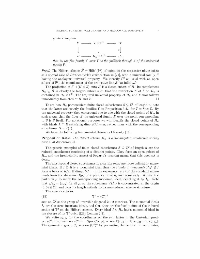
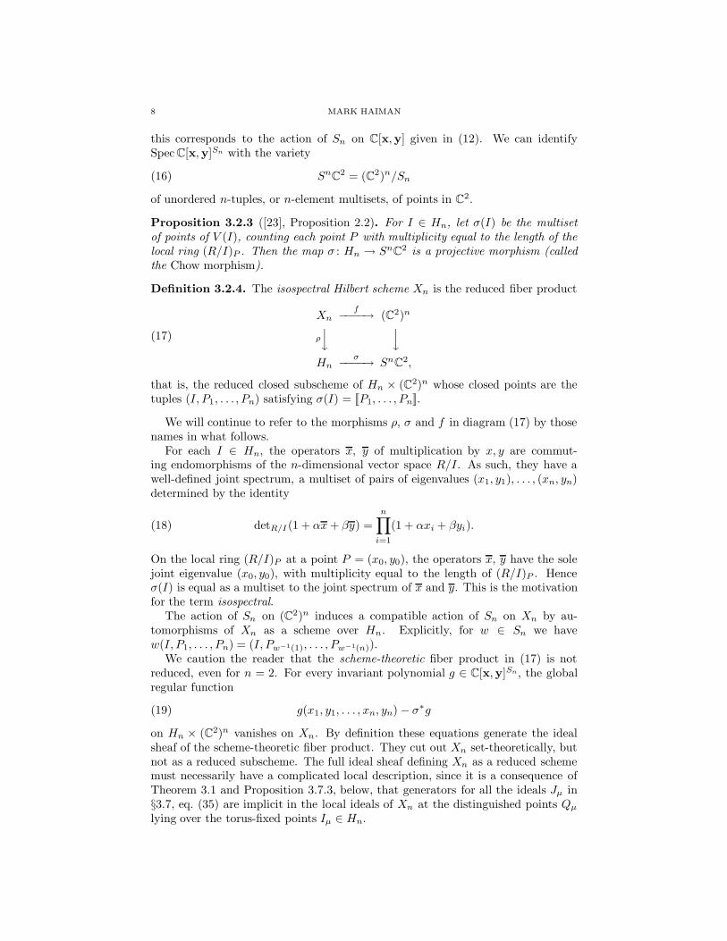


![arXiv:1610.03920v6 [math.RT] 7 Apr 2020Rational Cherednik algebras, Hilbert schemes, Nakajima quiver varieties, Calogero-Moser space, q-hook formula, wreath Macdonald polynomials,](https://static.documents.pub/doc/80x56/609a471d7515af559b217165/arxiv161003920v6-mathrt-7-apr-2020-rational-cherednik-algebras-hilbert-schemes.jpg)


