79
Hilbert transform: Mathematical theory and applications to signal processing M˚ ans Klingspor November 19, 2015 LiTH - MAT - EX - - 2015/09 - - SE

Hilbert transform: Mathematical theory and
applications to signal processing
Mans Klingspor
November 19, 2015
LiTH - MAT - EX - - 2015/09 - - SE

Hilbert transform: Mathematical theory andapplications to signal processing
Mans KlingsporLiTH - MAT - EX - - 2015/09 - - SE
Examensarbete: 30 hp
Level: A
Supervisor: Natan KruglyakMatematiska institutionen, Linkopings universitet
Examiner: Irina AsekritovaMatematiska institutionen, Linkopings universitet
Linkoping: November 2015

Contents
Acknowledgements 2
Abstract 3
Introduction 4
1 The Hilbert transform 101.1 Hilbert transform on the real line . . . . . . . . . . . . . . . . . . 101.2 Basic properties of the Hilbert transform . . . . . . . . . . . . . . 131.3 Hilbert transform and the Fourier transform . . . . . . . . . . . . 151.4 Hilbert transform of periodic functions . . . . . . . . . . . . . . . 221.5 Analytic representation of a signal . . . . . . . . . . . . . . . . . 231.6 Boundedness of the Hilbert transform . . . . . . . . . . . . . . . 271.7 Harmonic analysis . . . . . . . . . . . . . . . . . . . . . . . . . . 29
2 Hilbert transform and electrocardiogram 322.1 Basics of electrocardiography . . . . . . . . . . . . . . . . . . . . 322.2 Hilbert transform of the QRS complex . . . . . . . . . . . . . . . 322.3 Analysis of real ECG-signals . . . . . . . . . . . . . . . . . . . . . 362.4 Limitation of the method . . . . . . . . . . . . . . . . . . . . . . 43
3 The Hilbert-Huang transform 453.1 An algorithm for decomposition . . . . . . . . . . . . . . . . . . . 453.2 Interpretation of the decomposition . . . . . . . . . . . . . . . . . 493.3 Trigonometric polynomials and the HHT . . . . . . . . . . . . . . 533.4 Nonstationary processes and the HHT . . . . . . . . . . . . . . . 573.5 Limitations of HHT . . . . . . . . . . . . . . . . . . . . . . . . . 60
3.5.1 End effects . . . . . . . . . . . . . . . . . . . . . . . . . . 603.5.2 Adjacent frequencies . . . . . . . . . . . . . . . . . . . . . 61
4 Hilbert transform and modulation 664.1 Introduction to Amplitude modulation . . . . . . . . . . . . . . . 664.2 Single-sideband modulation . . . . . . . . . . . . . . . . . . . . . 67
5 Discussion 725.1 Electrocardiogram . . . . . . . . . . . . . . . . . . . . . . . . . . 725.2 Hilbert-Huang transform . . . . . . . . . . . . . . . . . . . . . . . 72
References 74
1

Acknowledgements
I would like to thank my supervisor, professor Natan Kruglyak, for his invalu-able assistance and guidance. Also, I would like to thank my partner AmandaKarunayake for her support and patience. Last but not least, I would also liketo thank my family and friends.
2
Abstract
The Hilbert transform is a widely used transform in signal processing. In thisthesis we explore its use for three different applications: electrocardiography, theHilbert-Huang transform and modulation. For electrocardiography, we examinehow and why the Hilbert transform can be used for QRS complex detection.Also, what are the advantages and limitations of this method? The Hilbert-Huang transform is a very popular method for spectral analysis for nonlinearand/or nonstationary processes. We examine its connection with the Hilberttransform and show limitations of the method. Lastly, the connection betweenthe Hilbert transform and single-sideband modulation is investigated.
URL for electronic version:http://liu.diva-portal.org/smash/record.jsf?pid=diva2:872439
3

Introduction
The Hilbert transform is one of the most important operators in the field ofsignal theory. Given some function u(t), its Hilbert transform, denoted byH(u(t)), is calculated through the integral
H(u(t)) = limε→0
1
π
∫|s−t|>ε
u(s)
t− sds.
The Hilbert transform is named after David Hilbert (1862-1943). Its first usedates back to 1905 in Hilbert’s work concerning analytical functions in connec-tion to the Riemann problem. In 1928 it was proved by Marcel Riesz (1886-1969)that the Hilbert transform is a bounded linear operator on Lp(R) for 1 < p <∞.This result was generalized for the Hilbert transform in several dimensions (andsingular integral operators in general) by Antoni Zygmund (1900-1992) and Al-berto Calderon (1920-1998).
Mainly, the importance of the transform is due to its property to extend realfunctions into analytic functions. This property certainly induces a vast numberof applications, especially in signal theory, and obviously the Hilbert transformis not merely of interest for mathematicians.
This thesis revolves around an aim that is twofold:
(i) To acquire more knowledge about the Hilbert transform and some of itsapplications to signal processing.
(ii) To better understand why some important applications related to theHilbert transform, to this day, lack mathematical theory.
The thesis consists of two major parts. In the first part mathematical theoryof the Hilbert transform is included. These results are well-known but includedto provide a steady ground. In the second part, we consider three different ap-plications of the Hilbert transform. The applications that has been consideredare: a) Electrocardiography, b) Hilbert-Huang transform and c) modulation.The first two applications nowadays lacks mathematical theory despite numer-ous efforts. Thus, in this thesis, computer experiments have been carried out inorder to deduce limitations of these methods and also pave the way for futureresarch in these areas.
(a) Electrocardiography: The Hilbert transform is a widely used tool in inter-preting electrocardiograms (ECGs). In Figure 1 we can see a part of anECG-signal, ECG(t). A common task when dealing with ECG-signals is toextract the so called QRS complex which is the high peak seen in the graphof ECG(t) (see Figure 1). In this thesis we thoroughly explore a methodof detecting the QRS complex in a ECG signal, as suggested by [2]. Thismethod is very attractive since we are only required to calculate the Hilberttransform and no numerical derivation is involved.
4

With the Hilbert transform it is possible to expand a real valued signalinto a so called analytic signal.
Figure 1: A plot of ECG(t), representing a part of an ECG-signal.
z(t) = ECG(t) + i · H(ECG(t))
A parametric plot of z(t), that is, a plot of ECG(t) against H(ECG(t))reveals interesting things about the ECG(t). Looking at Figure 2, we seethat a main loop enclosing the origin is generated. In the thesis, we haveshown that if the QRS complex is high enough, it will always produce aclosed loop around the origin in the complex plane, distinguishable fromthe rest of the graph. Also, we have justified this using the fact that theQRS complex resembles a deformed sine wave. By looking at analytic sinewaves and deformed sine waves we have established that all type of sinewaves, if expanded to analytic signals, form loops enclosing the origin inthe complex plane. Thus, the QRS complex, which is a deformed sine wave,also produces enclosed loops in the complex plane.
In our experiments, a limitation was encountered that should be adressed.If the QRS complex to be detected is not high enough, the method doesnot work. When the QRS complex is too low, the analytic expansion of theQRS complex will not produce a single distinguishable main loop enclosingthe origin. It may either not be detected or other peaks in the ECG falselyinterpreted as an QRS complex we have found.
(b) The Hilbert-Huang transform: In time series analysis the Fourier transformis the dominating tool. However, this method is not good enough for non-stationary or nonlinear data. For this purpose, the Hilbert-Huang transform(HHT) was proposed in 1996 [10]. This method has gained popularity andis widely used in spectral analysis since it, in contrast to common ”Fourier
5

Figure 2: A plot of ECG(t) against H(ECG(t)).
methods”, suppose that frequency and amplitude of the harmonics are de-pendent on time. This is achieved by decomposing the time series into socalled intrinsic mode functions (IMFs). However, in spite of considerableefforts, the HHT to this day lacks mathematical framework and the methodis entirely empirical. Thus, the investigation of this method is carried outnumerically in this thesis to try to understand how the method works andwhat limitations are inherit.
In the thesis, we state and investigate the following conjecture
Conjecture. Suppose X(t) is a time series and its Hilbert-Huangtransform is a decomposition given by
X(t) =
n∑i=1
ci(t) + rn(t).
Then the IMFs, ck(t), are decreasing in complexity as k increases. Thatis, given ck(t) and ck+1(t), then ck(t) has more zero crossings comparedto ck+1(t) for 1 ≤ k ≤ n− 1.
Note that more zero crossing means that ck(t) has higher frequency contentcompared to ck+1(t). To check the validity of this conjecture, consider forexample a process given by
X(t) =
sin (t), 0 ≤ t ≤ 10π
sin (t) + sin (10t), 10π ≤ t ≤ 100
which also can be seen in Figure 3). In this case we have some background
6

process given by sin (t). While the ”new” process, given by sin (10t), isdominating the background process is still active. Obviously, this is a non-stationary situation and therefore the HHT could be very useful in acquiringthe harmonics.
Figure 3: Plot of X(t).
According to the conjecture, we should for X(t) expect the following IMFs.
c1(t) =
sin (t), 0 ≤ t ≤ 10π
sin (10t), 10π ≤ t ≤ 100
c2(t) =
0, 0 ≤ t ≤ 10π
sin (t), 10π ≤ t ≤ 100
where the component with the highest frequency in each interval. Theactual IMFs, acquired by calculation and denoted by c1(t) and c2(t) can beseen in Figure 4.
7
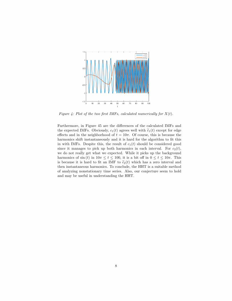
Figure 4: Plot of the two first IMFs, calculated numerically for X(t).
Furthermore, in Figure 45 are the differences of the calculated IMFs andthe expected IMFs. Obviously, c1(t) agrees well with c1(t) except for edgeeffects and in the neighborhood of t = 10π. Of course, this is because theharmonics shift instantaneously and it is hard for the algorithm to fit thisin with IMFs. Despite this, the result of c1(t) should be considered goodsince it manages to pick up both harmonics in each interval. For c2(t),we do not really get what we expected. While it picks up the backgroundharmonics of sin (t) in 10π ≤ t ≤ 100, it is a bit off in 0 ≤ t ≤ 10π. Thisis because it is hard to fit an IMF to c2(t) which has a zero interval andthen instantaneous harmonics. To conclude, the HHT is a suitable methodof analyzing nonstationary time series. Also, our conjecture seem to holdand may be useful in understanding the HHT.
8

Figure 5: Plot of the difference between the calculated IMFs and the expectedIMFs for X(t). That is, c1(t)− c1(t) and c2(t)− c2(t)
.
As was seen through the numerical investigations, the method works wellas conjectured in analyzing nonstationary and nonlinear data. However,one should be aware of these shortcomings in order to interpret the resultcorrectly. This is especially the case if in a time series there are frequencycomponents that are close to each other (adjacent frequencies). The resultis that the algorithm fails to distinguish between these distinct frequenciesand this we have investigated thoroughly; both by an example and a morequantative approach. Also, since the method is carried out numerically,finite signals are being considered. The result of this are so called endeffects in the IMFs.
(c) Modulation: Transmitting a bandlimited signal, m(t), is usually done ina frequency band centered around some frequency fc. This is fairly easyaccomplished by using modulation
mAM (t) = m(t) · cos (2πfct).
Inherently, this method has a weakness, namely, the frequency content ofMAM (f) = F(mAM (t)) is symmetrically doubled around fc. One way ofrefining the method is by using the Hilbert transform and properties ofanalytic signals. This refined modulation is given by
mSSB(t) = m(t) · cos (2πfct) +H(m(t)) · sin (2πfct).
In this section, this refined modulation will be derived in a clear manner.
For the numerical experiments MATLAB R2015a has been used. This version ofMATLAB has an inbuilt algorithm hilbert that performs the Hilbert transformnumerically. An algorithm for the Hilbert-Huang transform, created by Tan, A.in 2008, was downloaded from MATLAB Central [18].
9

1 The Hilbert transform
1.1 Hilbert transform on the real line
Definition 1.1. (Hilbert transform on R). Let x(t) ∈ Lp(R) be afunction for 1 ≤ p < ∞. Then H(x(t)) is the Hilbert transform of x(t)given by
H(x(t)) =1
πPV
∫ ∞−∞
x(s)
t− sds
Where ”PV ” is the Cauchy Principal Value of the integral.
For the Hilbert transform the Cauchy Principal Value is necessary in order tohandle the singularity at s = t. The Cauchy Principal Value is, in this context,utilized in the manner as follows [4].
1
πPV
∫ ∞−∞
x(s)
t− sds = lim
ε→0+
1
π
∫|t−s|≥ε
x(s)
t− sds
It is not obvious that this integral converges and consequently the Hilbert trans-form is well-defined. This issue will be revisited and adressed in a later section.
Example 1.2. The Hilbert transform for a constant function x(t) = c is easyto calculate using the definition
H(c) =1
πPV
∫ ∞−∞
c
t− sds =
c
πPV
∫ ∞−∞
1
t− sds = 0
The last equality is due to the integrand 1/(t− s) being an odd function over asymmetric interval around s = t. Hence, H(c) = 0 for any constant c.
Of course, it is not always this easy and straight forward to calculate the Hilberttransform. For more advanced functions we need to resort to techniques fromcomplex analysis in order to handle the integral. These techniques includecontour integrals in the complex plane and the residue theorem. Obviously, itis the singularity in x = t on the real line we need to take care of. For this andother purposes, the following lemmas are very useful.
Lemma 1.3. Let f(z) be analytic in some neighborhood of z0 where it hasa simple pole and Cε is a circular arc defined by Cε : z = z0 + ε · eiϕ withϕ : ϕ1 → ϕ2, then
limε→0+
∫Cε
f(z)dz = i(ϕ2 − ϕ1) · Resz=z0
f(z)
10

Proof. Since f(z) has a simple pole at z = z0 we can express its Laurentexpansion in some punctured neighborhood around z0.
f(z) =a−1z − z0
+
∞∑n=0
an(z − z0)n
Let g(z) =∑∞n=0 an(z − z0)n. Breaking up the integral into parts we get∫
Cε
f(z)dz = a−1
∫Cε
1
z − z0dz +
∫Cε
g(z)dz (1)
In said neighborhood around z0 the function g(z) is analytical and bounded so|g(z)| ≤M for some constant M . Using estimations we get∣∣∣∣∫
Cε
g(z)dz
∣∣∣∣ ≤M · (ϕ2 − ϕ1)ε→ 0 as ε→ 0+
For the other integral we get, using the paremetrization stated in the theorem∫Cε
1
z − z0dz =
∫ ϕ2
ϕ1
1
εeiϕεieiϕdϕ = i
∫ ϕ2
ϕ1
dϕ = i(ϕ2 − ϕ1)
From this and the fact that a−1 = Resz=z0
f(z) we get in (1) by evaluating limits
limε→0+
∫Cε
f(z)dz = a−1 · i(ϕ2 − ϕ1) + 0 = i(ϕ2 − ϕ1) · Resz=z0
f(z)
And the proof is thus complete.
Remark 1.4. In the case of the Hilbert transform, this simple pole will alwaysbe on the real line at the point z = t for a fixed t. To avoid this pole, a smallsemi-circle in either half-plane with ϕ1 = π and ϕ2 = 0 will suffice.
Lemma 1.5. (Jordan’s lemma). If C+R is the semicircle z = Reiϕ,
ϕ : 0→ π in the upper halfplane, a > 0 and R > 0, then∫C+R
|eiaz||dz| ≤ π
a
Proof. With the parameterization z = Reiϕ = R cosϕ+iR sinϕ we get |eiaz| =|eia(x+iy)| = |eiax−ay| = e−ay = e−aRsinϕ and |dz| = |iReiϕdϕ| = Rdϕ.∫
C+R
|eiaz||dz| =∫ π
0
e−aR sinϕRdϕ(1)= 2
∫ π/2
0
e−aR sinϕRdϕ
(2)
≤∫ π/2
0
e−aR·2ϕ/πRdϕ = −πa
[e−aR·2ϕ/π
]ϕ=π/2ϕ=0
=π
a(1− e−aR)
(3)
≤ π
a
11

The equality (1) is because sinϕ is symmetric around ϕ = π/2. Furthermore,since sinϕ is concave in the interval 0 ≤ ϕ ≤ π/2 its graph lies totally abovea straight line connecting its endpoints. Therefore, we have that sinϕ ≥ 2ϕ/πwhen 0 ≤ ϕ ≤ π/2 and hence inequality (2) holds. Of course, in order for (3)to hold we must have that a > 0 [9].
Example 1.6. Let x(t) = eiωt where ω is some real parameter. This is an com-plex exponential function and we would like to calculate its Hilbert transformwhich is defined by the integral
H(eiωt)(t) =1
πPV
∫ ∞−∞
eiωs
t− sds (2)
Start by looking at the case ω > 0. In order to calculate the integral we will haveto use techniques from complex analysis with contour integrals in the complexplane.
Define f(z) = 1/π · eiωz/(t − z) and the contour C = C+R + L2
ε,R + Cε + L1ε,R
which is closed and positively oriented. C+R is a semicircle with radius R in
the upper half-plane with the parameterization z = Reiϕ, ϕ : 0 → π. L1ε,R is a
straight line from z = −R to z = t− ε on the real line. Cε is a semicircle withradius ε in the upper half-plane with the parameterization z = ε · eiϕ, ϕ : π → 0.L2ε,R is the straight line from z = t + ε to z = R on the real line. A sketch of
the contour C is provided in Figure 6.
Figure 6: Sketch of the contour C. The contour is positively oriented.
Since f(z) is analytical both on and inside the contour C we have∫C
f(z)dz = 0
because of Cauchy’s integral theorem. Breaking up the integral thus yields∫L1ε,R+L2
ε,R
f(z)dz = −∫C+R
f(z)dz −∫Cε
f(z)dz (3)
12

Because ω > 0 and C+R is in the upper half-plane Jordan’s lemma gives us∣∣∣∣∣
∫C+R
f(z)dz
∣∣∣∣∣ ≤∫C+R
|f(z)||dz| =∫C+R
|eiωz||π(t− z)|
|dz| ≤ 1
π· 1
|R− t|
∫C+R
|eiωz||dz|
≤ 1
π· 1
|R− t|· π
2=
1
2· 1
|R− t|Furthermore, for the integral over the contour Cε we get by Lemma 1.3∫
Cε
f(z)dz = i(0− π) · Resz=t
f(z) = −iπ ·(eiωt
−π
)= ieiωt
Of course, the integral over the contour L1ε,R + L2
ε,R in (2) coincide with the
integral in (1) when R→∞ and ε→ 0+. For a fixed t, applying said limits andfor ω > 0 in (2) yield
1
πPV
∫ ∞−∞
eiωt
t− sds = −0− ieiωt = −ieiωt, ω > 0
For the case ω < 0 one may use the same technique as above with the execeptionthat the contours C+
R and Cε are instead semicircles in the lower half-plane. Thiswould for ω < 0 simply give us
1
πPV
∫ ∞−∞
eiωt
t− sds = ieiωt, ω < 0
For ω = 0 the complex exponential function is simply a constant and thus itsHilbert transform becomes 0 (as shown in Example 5.1) . Consequently, we mayconclude that for all ω ∈ R
H(eiωt) = −i sgn (ω)eiωt
This important result concludes this example.
1.2 Basic properties of the Hilbert transform
Theorem 1.7. Let y(t) = H(x(t)), y1(t) = H(x1(t)), y2(t) = H(x2(t))and let a, a1, a2 be some arbitrary constants. Then the Hilbert transformsatisifies the following basic properties:
(i) Linearity: H(a1x1(t) + a2x2(t)) = a1H(x1(t)) + a2H(x2(t))
(ii) Time shift: H(x(t− a)) = y(t− a)
(iii) Scaling: H(x(at)) = y(at), a > 0
(iv) Time reversal: H(x(−at)) = −y(−at), a > 0
(v) Derivative: H(x′(t)) = y′(t)
13

Proof: Property (i) follows directly from the fact that the integral itself is anlinear operation. Properties (ii)-(iv) can all be shown by a trivial change ofvariables. Property (v), which requires differentiability, will be shown later.
Example 1.8. With the properties above we may calculate the Hilbert trans-forms of the basic trigonometric functions. Suppose ω > 0.
H(cos(ωt)) = H(eiωt + e−iωt
2
)=H(eiωt) +H(ei(−ω)t)
2
=−i sgn (ω)eiωt − i sgn (−ω)ei(−ω)t
2
=−ieiωt − ie−iωt
2=eiωt − e−iωt
2i= sin (ωt)
H(sin(ωt)) = H(
cos(ωt− π
2
))= sin
(ωt− π
2
)= − cos(ωt)
In conclusion, if ω > 0 (which usually is the case) then H(cos(ωt)) = sin (ωt)and H(sin(ωt)) = − cos(ωt). By the time reversal property, if ω < 0 thenH(cos(ωt)) = − sin (ωt) and H(sin(ωt)) = −(− cos(ωt)) = cos(ωt). Written ina more compact form, for all ω ∈ R we have
H(cos(ωt)) = sgn (ω) sin (ωt)
H(sin(ωt)) = − sgn (ω) cos (ωt)
which are the Hilbert transforms for the basic cosine and sine-functions.
What properties does the Hilbert transform exhibit for even and odd functions?The following theorem gives us the answer.
Theorem 1.9. (Even and odd functions). Suppose f(t) has a well-defined Hilbert transform and that f(t) is either even or odd. Then, thefollowing holds
(i) If f(t) is even, its Hilbert transform is an odd function
(ii) If f(t) is odd, its Hilbert transform is an even function
Proof. From the definition of the Hilbert transform it follows that
H(f(t)) =1
πPV
∫ ∞−∞
f(s)
t− sds =
1
πPV
∫ ∞0
(f(s)
t− s+f(−s)t+ s
)ds
14

If f(t) is an even function, that is, f(−t) = f(t) we get
H(f(t)) =1
πPV
∫ ∞0
(f(s)
t− s+f(s)
t+ s
)ds
=1
πPV
∫ ∞0
((t+ s)f(s) + (t− s)f(s)
t2 − s2
)ds
=2t
πPV
∫ ∞0
f(s)
t2 − s2ds
and if f(t) is an odd function, that is, f(−t) = −f(t) we get
H(f(t)) =1
πPV
∫ ∞0
(f(s)
t− s− f(s)
t+ s
)ds
=1
πPV
∫ ∞0
((t+ s)f(s)− (t− s)f(s)
t2 − s2
)ds
=2
πPV
∫ ∞0
sf(s)
t2 − s2ds.
From these two expressions the theorem follows and the proof is complete.
1.3 Hilbert transform and the Fourier transform
It is easy to see that the Hilbert transform y(t) = H(x(t)) actually can beinterpreted as an convolution between x(t) and 1/(πt). This requires, however,a rigorous proof. For this purpose, we need a couple of important theoremsfrom functional analysis [11].
Theorem 1.10. (Holder’s inequality). Suppose f(t) ∈ Lp(R), g(t) ∈Lq(R) where 1/p+ 1/q = 1 for 1 ≤ p, q ≤ ∞. Then,
||fg|| ≤ ||f ||p||g||q
Theorem 1.11. If f(t) ∈ Lp(R), 1 ≤ p ≤ ∞ and g(t) ∈ L1(R), then theconvolution (f ∗ g)(t) is in Lp(R) and
‖f ∗ g‖p ≤ ‖f‖p‖g‖1
Proof. For the proof we will consider three different cases, namely p = 1,p =∞ and 1 < p <∞.
15

(i) p = 1: This case is trivial since
‖f ∗ g‖1 =
∥∥∥∥∫Rf(s)g(t− s)ds
∥∥∥∥ =
∫R
∣∣∣∣∫Rf(s)g(t− s)ds
∣∣∣∣dt≤∫R
∫R|f(s)||g(t− s)|dsdt =
∫R|f(s)|
∫R|g(t− s)|dtds
=
∫R|f(s)| · ‖g‖1ds = ‖g‖1
∫R|f(s)|ds = ‖g‖1‖f‖1 = ‖f‖1‖g‖1
(ii) p =∞: As a reminder, ‖f‖∞ = supt|f(t)| <∞ if f(t) ∈ L∞(R).
||f ∗ g||∞ = supt
∣∣∣∣∫Rf(s)g(t− s)ds
∣∣∣∣ = supt
∣∣∣∣∫Rf(t− s)g(s)ds
∣∣∣∣≤ sup
t
∫R|f(t− s)||g(s)|ds =
∫R
supt|f(t− s)||g(s)|ds
=
∫R‖f‖∞|g(s)|ds = ‖f‖∞
∫R|g(s)|ds = ‖f‖∞‖g‖1
(iii) 1 < p <∞: Let q satisfy 1p + 1
q = 1.
|(f ∗ g)(t)| =∣∣∣∣∫
Rf(s)g(t− s)ds
∣∣∣∣ ≤ ∫R|f(s)||g(t− s)|ds
=
∫R|f(s)||g(t− s)|1/p|g(t− s)|1/qds
(∗)≤(∫
R|f(s)|p|g(t− s)|ds
)1/p(∫R|g(t− s)|ds
)1/q
= ‖g‖1/q1
(∫R|f(s)|p|g(t− s)|ds
)1/p
Where (∗) is because of Holder’s inequality. Taking the Lp(R)-norm ofboth sides yields
‖f ∗ g‖p ≤ ‖g‖1/q1
(∫R
∫R|f(s)|p|g(t− s)|dsdt
)1/p
= ‖g‖1/q1
(∫R|f(s)|p
∫R|g(t− s)|dtds
)1/p
= ‖g‖1/q1
(∫R|f(s)|p‖g‖1ds
)1/p
= ‖g‖1/q1 ‖g‖1/p1
(∫R|f(s)|pds
)1/p
= ‖g‖1/p+1/q1 ‖f‖p = ‖f‖p‖g‖1
With cases (i), (ii) and (iii) proved the proof is thus complete.
16

Theorem 1.12. Suppose x(t) ∈ Lp(R), 1 < p ≤ 2 and F(x(t)) is theFourier transform of x(t). Then the Fourier transform of H(x(t)) is givenby F(H(x(t))) = (−i sgn (f)) · F(x(t)).
Proof. Define the function
uε,R(t) =
1πt , 0 < ε < |t| < R <∞0 otherwise
and let Hε,R be a truncated Hilbert transform. Clearly
Hε,R(x(t)) =1
π
∫ε<|t|<R
x(s)
t− sds =
∫ ∞−∞
x(s)uε,R(t− s)ds = (x ∗ uε,R)(t)
is a convolution that makes sense since uε,R ∈ L1(R) and x(t) ∈ Lp(R), 1 <p ≤ 2. Then, according to Theorem 5.10, ‖x ∗ uε,R‖1 ≤ ‖x‖p‖uε,R‖1. This alsomeans that Hε,R(x(t)) ∈ Lp(R), 1 < p ≤ 2. The Fourier transform of Hε,R(x(t))is given by
F(Hε,R(x(t))) = F ((x ∗ uε,R)(t)) = F(x(t)) · F(uε,R(t))
and we need to calculate F(uε,R(t)).
F(uε,R(t)) =
∫ε<|t|<R
e−2πift
πtdt =
∫ −ε−R
e−2πift
πtdt+
∫ R
ε
e−2πift
πtdt
= −∫ R
ε
e2πift
πtdt+
∫ R
ε
e−2πift
πtdt = − 1
π
∫ R
ε
e2πift − e−2πift
tdt
= −2i
π
∫ R
ε
sin 2πft
tdt = −2i sgn (2πf)
π
∫ 2π|f |R
2π|f |ε
sin t
tdt
= −2i sgn (f)
π
∫ 2π|f |R
2π|f |ε
sin t
td
The integral at the end has the limit π/2 as ε→ 0+, R→∞. This can be shownquite easily just using earlier employed techniques with contour integrals in thecomplex plane. Obviosuly, we have that F(uε,R(t)) → −i sgn (f) as ε → 0+,R→∞ for every real value of f .
Since F(uε,R(t))→ −i sgn (f) as ε→ 0+, R→∞ we have that |F(uε,R(t))| ≤ Cfor some C depending on the values of ε and R. We can now show that
H(x(t)) = limε→0+
limR→∞
Hε,R(x(t)) = F−1 (−i sgn (f) · F(x(t)))
17

by making use of Lebesgue’s theorem of dominated convergence. For 1 < p ≤ 2
limε→0+
limR→∞
‖Hε,R(x(t))−F−1 (−i sgn (f) · F(x(t))) ‖p(∗)= lim
ε→0+limR→∞
‖F(Hε,R(x(t)))− (−i sgn (f) · F(x(t)))‖p
= limε→0+
limR→∞
‖F(x(t)) · F(uε,R(t))− (−i sgn (f) · F(x(t)))‖p
= limε→0+
limR→∞
‖(F(uε,R(t))− (−i sgn (f))) · F(x(t))‖p = 0
where (∗) is because of Parseval’s identity. Thus we have established the limitabove (in the sense of the Lp norm). Now, by just taking the Fourier transformof both sides we get because of the Fourier inversion theorem that
F(H(x(t))) = (−i sgn (f)) · F(x(t))
and the proof is complete.
Remark 1.13. Why does the theorem not hold for the case p = 1? Becausex(t) ∈ L1(R) does not necessarily imply that H(x(t)) ∈ L1(R). For example,let x(t) = χ[0,1](t) ∈ L1(R). Then its Hilbert transform is given by
H(x(t)) =1
πPV
∫ 1
0
1
t− sds =
1
πln
∣∣∣∣ t
t− 1
∣∣∣∣and clearly H(x(t)) /∈ L1(R. Therefore, the Fourier transform of H(x(t)) doesnot exist in the usual sense and the theorem does not hold. However, if bothx(t), H(x(t)) ∈ L1(R) then all steps in the proof are valid and the theoremholds even for p = 1.
With this relationship between the Hilbert transform and the Fourier transformwe may show various different properties of the Hilbert transform. We beginwith the differentiation property.
Theorem 1.14. (Differentiation). If x(t) ∈ Lp(R), 1 < p ≤ 2 is differ-entiable, then it holds that H(x′(t)) = d
dtH(x(t)).
Proof. By the differentation property of the Fourier transform and Theorem1.11 we get by some simple algebra
F(H(x′(t))) = (−i sgn (f)) · F(x′(t)) = (−i sgn (f)) · (2πif · F(x(t))
= 2πif · (−i sgn (f)) · F(x(t)) = 2πif · F(H(x(t)))
= F(d
dtH(x(t))
)
18

Through this, since they share the same Fourier transform, it is established thatH(x′(t)) = d
dtH(x(t)), thus the differentiation property of the Hilbert transform.
Another interesting property we can show is the inversion property.
Theorem 1.15. (Inversion). Suppose x(t) ∈ Lp(R), 1 < p ≤ 2. Then itholds that H(H(x(t)) = −x(t).
Proof. By using Theorem 1.11 twice we get
F(H(H(x(t)))) = (−i sgn (f)) · F(H(x(t)))
= (−i sgn (f)) · (−i sgn (f)) · F(x(t))
= i2 · (sgn (f))2 · F(x(t)) = −F(x(t)) = F(−x(t))
SinceH(H(x(t))) and −x(t) have the same Fourier transform almost everywherewe can conclude that H(H(x(t))) = −x(t) and the proof is complete.
In words, applying the Hilbert transform twice on a function x(t) it simplyyields −x(t) - the very same function except for a minus sign. Thus, if H is anHilbert operator the inverse is H−1 = −H.
Theorem 1.16. (Orthogonality). Suppose x(t) ∈ L2(R) is a purelyreal function with the Fourier transform, X(f) = F(x(t)). Then x(t) andH(x(t)) are orthogonal functions, that is∫ ∞
−∞x(t) · H(x(t))dt = 0
Proof. With Parseval’s identity and Theorem 1.11 we get∫ ∞−∞
x(t) · H(x(t))dt =
∫ ∞−∞
X(f) · (−i sgn (f) ·X(f))df
=
∫ ∞−∞
X(f) · i sgn (f) ·X(f)df
= i
∫ ∞−∞
sgn (f)|X(f)|2df.
Since x(t) is real it means that |X(f)| = |X(−f)| (more about this in section1.5). Therefore, sgn (f)|X(f)|2 is an odd function since sgn (f) is odd and
19

|X(f)|2 even. With the symmetric interval of integration, the integral is zeroand we have the desired result,∫ ∞
−∞x(t) · H(x(t))dt = 0
which means that x(t) and H(x(t)) are orthogonal functions. Proof is complete.
Remark 1.17. The differentiation, inversion and orthogonality properties ofthe Hilbert transform can be generalized for a broader class of functions.
For the general case, the Hilbert transform offer no shortcuts for calculatingthe Hilbert transform of products of functions. There is however a special casecovered by the so called Bedrosian’s theorem [4].
Theorem 1.18. (Bedrosian’s theorem). Suppose f(t) and g(t) haveFourier transforms F (f) and G(f), respectively, where F (f) = 0 for |f | > awith a > 0 and G(f) = 0 for |f | < a. Then
H(f(t)g(t)) = f(t)H(g(t))
Proof. Using the fact that H(eist) = −i sgn (s)eist for s ∈ R we have
H(f(t)g(t)) =H(∫ ∞−∞
F (u)e2πiutdu
∫ ∞−∞
G(v)e2πivtdv
)=H
(∫ ∞−∞
F (u)
∫ ∞−∞
G(v)e2πi(u+v)tdvdu
)=
∫ ∞−∞
F (u)du
∫ ∞−∞
G(v)H(e2πi(u+v)t)dv
=
∫ ∞−∞
F (u)du
∫ ∞−∞
G(v)(−i sgn (u+ v)e2πi(u+v)t)dv
=− i∫ ∞−∞
F (u)e2πiutdu
(∫ −a−∞
G(v)e2πivt sgn (u+ v)dv
+
∫ ∞a
G(v)e2πivt sgn (u+ v)dv
)
20

Make a change of variables in the inner integral, w = u+ v
H(f(t)g(t)) =− i∫ a
−aF (u)e2πiutdu
(∫ −a+u−∞
G(w − u)e2πi(w−u)t sgn (w)dw
+
∫ ∞a+u
G(w − u)e2πi(w−u)t sgn (w)dw
)=− i
∫ a
−aF (u)du
(∫ −a+u−∞
G(w − u)e2πiwt sgn (w)dw
+
∫ ∞a+u
G(w − u)e2πiwt sgn (w)dw
)For the first integral the integrand is non-zero when w − u < −a ⇐⇒ w <−a + u and for the second integral the integrand is non-zero when w − u >a ⇐⇒ w > a + u. Since −a < u < a the sign-function in each integral takesonly one value and we may simplify
H(f(t)g(t)) =− i∫ a
−aF (u)du
(−∫ −a+u−∞
G(w − u)e2πiwtdw
+
∫ ∞a+u
G(w − u)e2πiwtdw
)Make another change of variables, let y = w − u which gives
H(f(t)g(t)) =− i∫ a
−aF (u)du
(−∫ −a−∞
G(y)e2πi(y+u)tdy
+
∫ ∞a
G(y)e2πi(y+u)tdy
)=− i
∫ a
−aF (u)e2πiutdu
(−∫ −a−∞
G(y)e2πiytdy
+
∫ ∞a
G(y)e2πiytdy
)=
∫ a
−aF (u)e2πiutdu
(∫ −a−∞
(−i sgn (y))G(y)e2πiytdy
+
∫ ∞a
G(y)(−i sgn (y))e2πiytdy
)=f(t)
(∫ −a−∞
G(y)H(e2πiyt)dy +
∫ ∞a
G(y)H(e2πiyt)dy
)=f(t)H
(∫ −a−∞
G(y)H(e2πiyt)dy +
∫ ∞a
G(y)H(e2πiyt)dy
)=f(t)H(g(t))
And the proof is thus complete.
21

1.4 Hilbert transform of periodic functions
One can also define the Hilbert transform for periodic functions. Suppose u(t)is a function with period 2T - then it can be expressed as a Fourier series
u(t) =
∞∑n=−∞
cneπint/T
where each coeffiecent cn for a fixed n is given by
cn =1
2T
∫ T
−Tu(s)e−πins/T ds
With the facts that H(c) = 0 for any constant c and H(eist) = −i sgn (s)eist forany real number s we get
H(u(t)) = H (c0) +H
( ∞∑n=1
cneπint/T
)+H
(1∑
n=−∞cne
πint/T
)
= 0 +H
( ∞∑n=1
cneπint/T
)+H
( ∞∑n=1
cne−πint/T
)
=
∞∑n=1
cnH(eπint/T ) +
∞∑n=1
cnH(e−πint/T )
= −i∞∑n=1
cn
(eπint/T − e−πint/T
)= − i
2T
∞∑n=1
(∫ T
0
u(s)e−πins/T ds
)(eπint/T − e−2πint/T
)=−i2T
∫ T
−Tu(s)
( ∞∑n=1
eπin(t−s)/T − e−πin(t−s)/T)ds
=1
2T
∫ T
−Tu(s)
∞∑n=1
2 sin
(πn(t− s)
T
)ds
=1
2TPV
∫ T
−Tu(s) cot
(πt− s2T
)ds
The last equality is because of the identity
2
∞∑k=1
sin kx = cot(x
2
)which is valid in the sense of distributions [7]. Now, the following definition ofa periodic Hilbert transform makes sense.
22
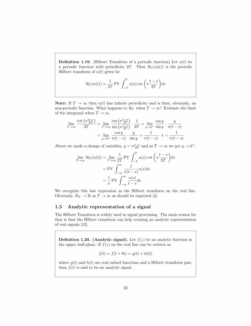
Definition 1.19. (Hilbert Transform of a periodic function) Let u(t) bea periodic function with periodicity 2T . Then HT (u(t)) is the periodicHilbert transform of u(t) given by
HT (u(t)) =1
2TPV
∫ T
−Tu(s) cot
(πt− s2T
)ds
Note: If T → ∞ then u(t) has infinite periodicity and is then, obviously, annon-periodic function. What happens to HT when T →∞? Evaluate the limitof the integrand when T →∞.
limT→∞
cot(π t−s2T
)2T
= limT→∞
cos(π t−s2T
)sin(π t−s2T
) · 1
2T= limy→0+
cos y
sin y· y
π(t− s)
= limy→0+
cos y
π(t− s)· y
sin y=
1
π(t− s)· 1 =
1
π(t− s)
Above we made a change of variables, y = π t−s2T and as T →∞ we get y → 0+.
limT→∞
HT (u(t)) = limT→∞
1
2TPV
∫ T
−Tu(s) cot
(πt− s2T
)ds
= PV
∫ ∞−∞
1
π(t− s)u(s)ds
=1
πPV
∫ ∞−∞
u(s)
t− sds
We recognize this last expression as the Hilbert transform on the real line.Obviously, HT → H as T →∞ as should be expected [4].
1.5 Analytic representation of a signal
The Hilbert Transform is widely used in signal processing. The main reason forthat is that the Hilbert transform can help creating an analytic representationof real signals [12].
Definition 1.20. (Analytic signal). Let f(z) be an analytic function inthe upper half-plane. If f(z) on the real line can be written as
f(t) = f(t+ 0i) = g(t) + ih(t)
where g(t) and h(t) are real-valued functions and a Hilbert transform pair,then f(t) is said to be an analytic signal.
23

Note that this is one of various ways to define an analytic signal. Not all analyticfunctions are analytic signals on the real line. One sufficient condition is that|f(z)| → 0 as |z| → ∞, Im z > 0 which is explored in the next theorem.
Theorem 1.21. Let f(z) be an analytic function for Im z ≥ 0 that vanishesin the upper half-plane (|f(z)| → 0 as |z| → ∞). Then, on the real linef(z) is an analytic signal and can be written as
f(t) = g(t) + iH(g(t))
where g(t) = Re f(t+ 0i) = u(t, 0) and H(g(t)) = Im f(t+ 0i) = v(t, 0) arereal valued functions.
Proof. Define the contour C like in Example 1.6. Then, since f(z) is analyticin the upper half-plane we have according to Cauchy’s integral theorem∫
C
f(z)
t− zdz = 0
since the integrand f(z)/(t − z) is analytical inside the contour. Breaking upthe integral in parts we get∫
L1ε,R+L2
ε,R
f(z)
t− zdz = −
∫C+R
f(z)
t− zdz −
∫Cε
f(z)
t− zdz
For the integral over the contour C+R we have that∣∣∣∣∣
∫C+R
f(z)
t− zdz
∣∣∣∣∣ ≤maxz∈C+
R
|f(z)|
|t−R|· πR =
π
|t/R− 1|· max0<ϕ<π
|f(Reiϕ)|
and since |f(z)| → 0 as |z| → ∞, Im z > 0 by assumption it therefore holds that|f(Reiϕ)| → 0 as R→∞ for 0 < ϕ < π. Thus, as R→∞∣∣∣∣∣
∫C+R
f(z)
t− zdz
∣∣∣∣∣→ π · 0 = 0
Looking on the integral over the the contour Cε, from Lemma 1.3, we have that∫Cε
f(z)
t− zdz = i(0− π) · Res
z=t
f(z)
t− z= −iπ · (−f(t)) = iπf(t)
Letting ε→ 0+, R→∞, dividing by π and parameterizing we get
1
πPV
∫ ∞−∞
f(s)
t− sds = −0− if(t) = −if(t)
24

We have that H(f(t)) = −if(t). Since f(z) is a complex and analytic functionwe can write f(z) = f(x+ iy) = u(x, y) + iv(x, y) where u(x, y) and v(x, y) arereal valued functions. On the real line (x = t, y = 0) we therefore get
H(f(t)) = H(u(t, 0) + iv(t, 0)) = H(u(t, 0)) + iH(v(t, 0)) = −if(t)
= −i(u(t, 0) + iv(t, 0)) = v(t, 0)− iu(t, 0)
Identifying real and imaginary parts we have that H(u(t, 0)) = v(t, 0) andH(v(t, 0)) = −u(t, 0). Thus, if we let g(t) = u(t, 0) we simply have f(t) =g(t) + iH(g(t)) and f(t) is an analytic signal.
Example 1.22. Let f(z) = eiωz for ω > 0. Clearly f(z) is analytic for Im z ≥ 0and since |f(z)| = |eiωz| = |eiω(x+iy)| = |e−ωy+iωx| = e−ωy → 0 as |z| → ∞,Im z > 0 we have that f(z) vanishes in the upper half-plane. Hence, on the realline f(z) is an analytic signal.
f(t) = f(t+ i0) = eiω(t+0i) = eiωt = cosωt+ i sinωt
In this case we have g(t) = cosωt and as should be expected H(g(t)) = sinωt.
Example 1.23. Let f(z) = 1a−iz for a > 0. The function is singular in the
point z = −ia and analytic everywhere else. Thus, in the upper half-plane f(z)is analytic and obviously decreases with the same rate as 1/|z|. Therefore, f(z)represents an analytic signal on the real line and we have that
f(t) = f(t+ 0i) =1
a− it=
a+ it
a2 + t2=
a
a2 + t2+ i
t
a2 + t2
and we have shown that H(
aa2+t2
)= t
a2+t2 and H(
ta2+t2
)= − a
a2+t2 for a > 0.
The following theorem we have esentially shown already but because of its use-fulness it is worthful to state in a clear manner.
Theorem 1.24. Suppose f(t) is an analytic signal. Then its Hilbert trans-form is given by H(f(t)) = −if(t).
Proof. See the proof of Theorem 1.21.
Theorem 1.25. Suppose f1(t) and f2(t) are analytic signals. Then it holdsthat H(f1(t)) · f2(t) = f1(t) · H(f2(t)).
Proof. The proof is just a matter of rearranging and using Theorem 1.13.
H(f1(t)) · f2(t) = −if1(t) · f2(t) = f1(t) · (−if2(t)) = f1(t) · H(f2(t))
25

Theorem 1.26. Let f(t) = g(t) + iH(g(t)) be an analytic signal. Then itsFourier transform, F (f), is given by
F (f) = (1 + sgn (f)) ·G(f) =
2G(f), f > 0
G(0), f = 0
0, f < 0
Proof. By using Theorem 1.8 we readily get
F (f) = F(f(t)) = F(g(t) + iH(g(t))) = F(g(t)) + i · F(H(g(t)))
= G(f) + i · (−i sgn (f)) ·G(f)) = (1 + sgn (f)) ·G(f)
and the proof is complete. Note that for the sign function we have sgn (0) = 0.
This theorem is very interesting since the function g(t) is real. Because g(t)is purely real and that conjugation is a linear operation we have that
G(f) =
∫ ∞−∞
g(t)e−2πiftdt =
∫ ∞−∞
g(t)e−2πiftdt =
∫ ∞−∞
g(t)e−2πiftdt
=
∫ ∞−∞
g(t)e2πiftdt =
∫ ∞−∞
g(t)e−2πi(−f)tdt = G(−f)
and thus G(f) has Hermitian symmetry since G(−f) = G(f). In particularit holds that |G(f)| = |G(−f)| since |G(f)| = |G(f)|. Consequently, when weconsider the amplitude spectrum |G(f)|, it is an even function with symmetryaround f = 0. Because of these symmetries, it is clearly sufficient to considerG(f) for f ≥ 0. This is one of many advantages with analytic signals - theycarry only positive frequency components and discard the negative frequenciessince they are superfluous for real signals [12].
Example 1.27. Consider g(t) = cosωt for ω > 0. As has been seen already wecan expand g(t) into an analytic signal.
f(t) = cosωt+ iH(cosωt) = cosωt+ i sinωt = eiωt
As is known, G(f) = F(cos (ωt)) = 12
(δ(f − ω
2π
)+ δ
(f + ω
2π
)). As expected,
because g(t) is purely real G(f) has Hermitian symmetry. Also, because G(f)is purely real as well, G(f) = G(f) and so G(−f) = G(f). For the analyticsignal we consequently get the Fourier transform
F (f) =
2G(f), f > 0
G(0), f = 0
0, f < 0
=
δ(f − ω
2π
)+ δ
(f + ω
2π
), f > 0
0, f = 0
0, f < 0
26
Of course, δ(f − ω
2π
)+ δ
(f + ω
2π
)= δ
(f − ω
2π
)for f > 0. To conclude, we
have that F (f) = δ(f − ω
2π
)and as expected F (f) = 0 for f < 0. The term
δ(f + ω
2π
)is discarded but no information is lost since the same information is
carried in the term δ(f − ω
2π
).
To transmit the signal g(t) completely one needs to consider the frequencycomponents in − ω
2π ≤ f ≤ ω2π , resulting in ω
2π −(− ω
2π
)= ω
π as the smallestpossible bandwidth. In contrast, for f(t) is is enough to consider frequencycomponents for 0 ≤ f ≤ ω
2π and because ω2π − 0 = ω
2π = 12 ·
ωπ the bandwidth
required for complete transmission is halved.
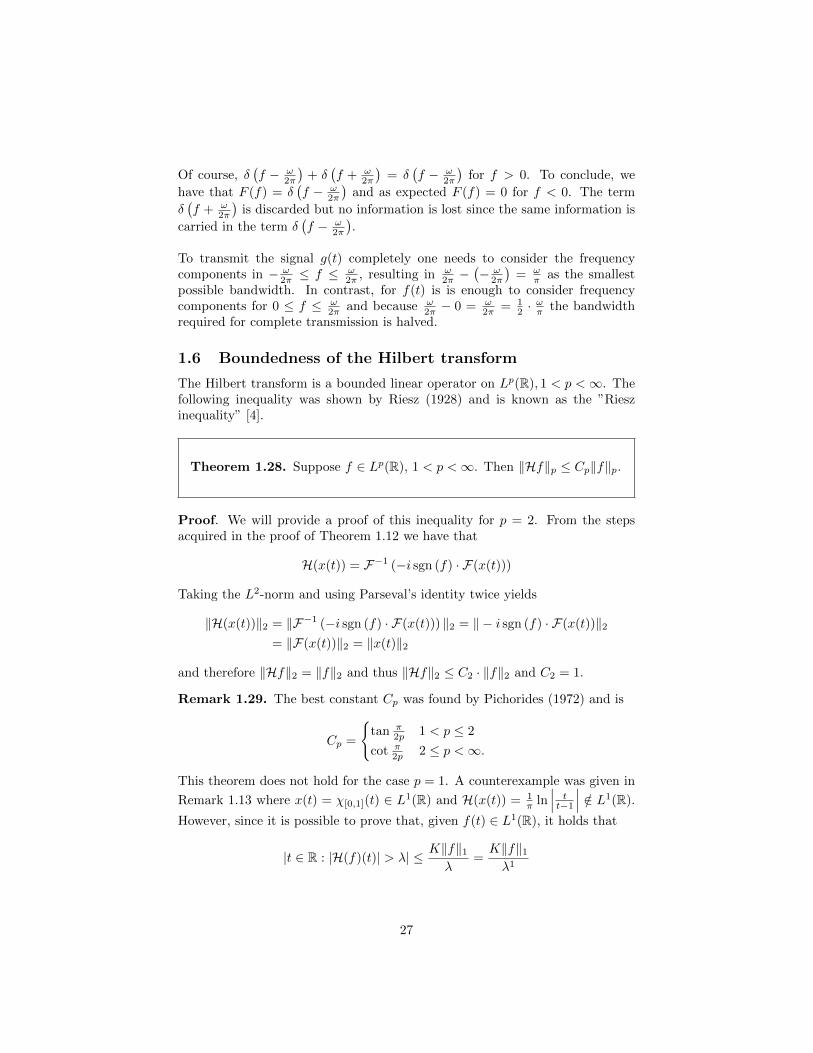
1.6 Boundedness of the Hilbert transform
The Hilbert transform is a bounded linear operator on Lp(R), 1 < p <∞. Thefollowing inequality was shown by Riesz (1928) and is known as the ”Rieszinequality” [4].
Theorem 1.28. Suppose f ∈ Lp(R), 1 < p <∞. Then ‖Hf‖p ≤ Cp‖f‖p.
Proof. We will provide a proof of this inequality for p = 2. From the stepsacquired in the proof of Theorem 1.12 we have that
H(x(t)) = F−1 (−i sgn (f) · F(x(t)))
Taking the L2-norm and using Parseval’s identity twice yields
‖H(x(t))‖2 = ‖F−1 (−i sgn (f) · F(x(t))) ‖2 = ‖ − i sgn (f) · F(x(t))‖2= ‖F(x(t))‖2 = ‖x(t)‖2
and therefore ‖Hf‖2 = ‖f‖2 and thus ‖Hf‖2 ≤ C2 · ‖f‖2 and C2 = 1.
Remark 1.29. The best constant Cp was found by Pichorides (1972) and is
Cp =
tan π
2p 1 < p ≤ 2
cot π2p 2 ≤ p <∞.
This theorem does not hold for the case p = 1. A counterexample was given in
Remark 1.13 where x(t) = χ[0,1](t) ∈ L1(R) and H(x(t)) = 1π ln
∣∣∣ tt−1
∣∣∣ /∈ L1(R).
However, since it is possible to prove that, given f(t) ∈ L1(R), it holds that
|t ∈ R : |H(f)(t)| > λ| ≤ K‖f‖1λ
=K‖f‖1λ1
27
for some K > 0, the Hilbert operator H is said to be of weak type of (1, 1) Thisspace is sometimes written as L1,w(R) equipped with the following norm
‖f‖L1,w = supλ>0
λ · |t ∈ R : |f(t)| > λ|.
The following theorem summarizes the result [4].
Theorem 1.30. Suppose f(t) ∈ L1(R). Then H(f(t)) ∈ L1,w(R).
For completeness, let us take a look at the multidimensional Hilbert transformand an inequality due to Alberto Calderon and Antoni Zygmund that impliesboundedness. However, first a definition of the n-dimensional Hilbert transformis needed. It is very straightforward [5].
Definition 1.31. The n-dimensional Hilbert transform of f(t) =f(t1, ..., tn) is given by
Hn(f(t)) = limε1→0+
... limεn→0+
∫D1
...
∫Dn
f(s1, ..., sn)
n∏j=1
1
(xj − sj)ds1...dsn
where Dk is given by |xk − sk| > εk.
Remark 1.32. Note that the Cauchy Principal Value is applied on each andeveryone of the integrals. For the case n = 1, we acquire the ”normal”, one-dimensional Hilbert transform.
For the n-dimensional Hilbert transform a result like Riesz inequality is valid.This inequality is known as the Calderon-Zygmund inequality.
Theorem 1.33. (Calderon-Zygmund inequality). Let f(t) ∈ Lp(En)with 1 < p <∞. Then
‖Hnf‖p ≤ Cp,n‖f‖p
where the constant Cp,n is only dependent on n and p.
By this theorem it follows that Hn is a bounded linear operator on Lp(Rn) for1 < p <∞.
28

1.7 Harmonic analysis
The Hilbert transform is a particular case of the so called singular integraloperators studied by Calderon and Zygmund. This is closely related to theDirichlet problem. This problem will be briefly discussed in this section.
Definition 1.34. (Dirichlet problem). Suppose we are looking for aharmonic function φ that is continuous and harmonic on a domain Ω and φ= f on ∂Ω where f is continuous. This problem is called Dirichlet problem.
Figure 7: A sketch of the Dirichlet problem for some region Ω.
If Ω is the upper half-plane and f(t) is the function on the real line, we haveseen that the Hilbert transform is a helpful tool to expand f(t) to an analyticfunction F (t) given by
F (t) = f(t) + iH(f(t))
where F (t) is an analytic function on the real line, that is, F (z) is an analyticfunction and F (t) = F (t+ 0i). Since F (z) is analytic, it can be written as
F (z) = F (t+ iy) = φ(t, y) + iψ(t, y)
where φ, ψ are harmonic functions. If f(t) ∈ L2(R) as y → 0, φ(t, y) → f(t)almost everywhere. The question is now, how can an harmonic function φ(x, y)be derived from f(t) if Ω is the upper half-plane?
Suppose Ω is the upper half-plane and f = φ + iψ is analytic in Ω. Also,suppose C = C+
R + LR is a positively contour in the upper half-plane (given inFigure 8). Then, if z is a point in the upper half-plane, we have according toCauchy’s integral formula
f(z) =1
2πi
∫C
f(ζ)
ζ − zdζ.
29

Furthermore, because z is outside the contour, it holds that
1
2πi
∫C
f(ζ)
ζ − zdζ = 0
thus yielding
f(z) =1
2πi
∫C
f(ζ)
ζ − zdζ − 1
2πi
∫C
f(ζ)
ζ − zdζ =
1
2πi
∫C
f(ζ)(z − z)(ζ − z)(ζ − z)
dζ.
Note that z − z = 2i Im z. Now, suppose |f(z)| ≤M , then on C+R we have∣∣∣∣∣ 1
2πi
∫C+R
f(ζ)(z − z)(ζ − z)(ζ − z)
dζ
∣∣∣∣∣ =Im z
π·
∣∣∣∣∣∫C+R
f(ζ)
(ζ − z)(ζ − z)dζ
∣∣∣∣∣≤ Im z
π
M
(R− |z|)2· πR
Thus, letting R→∞ and z = x+ iy yields
f(z) = f(x+ iy) =1
2πi
∫ ∞−∞
f(t) · 2i Im z
(t− z)(t− z)dt =
y
π
∫ ∞−∞
f(t)
(t− x)2 + y2dt
since the integral vanishes over C+R . Furthermore
f(x+ iy) = φ(x, y) + iψ(x, y) =y
π
∫ ∞−∞
φ(t, 0) + iψ(t, 0)
(t− x)2 + y2dt.
By taking real parts of both sides we have that
φ(x, y) =y
π
∫ ∞−∞
φ(t, 0)
(t− x)2 + y2dt
and in the integral the so called Poisson kernel is present. This expression isknown as the Poisson integral formula and it may be further generalized. Thisgeneralization is found in Theorem 1.35 and is the solution of the Dirichletproblem in the upper half-plane.
Figure 8: The contour C = C+R + LR.
30
Theorem 1.35. The solution of a Dirichlet problem in the upper half-planewhere φ(x, y) attains the values f(x) on the real line is given by
φ(x, y) =y
π
∫ ∞−∞
f(s)
(t− s)2 + y2ds
31
2 Hilbert transform and electrocardiogram
In the field of medicine, one of the most important tool is a so called electro-cardiaogram, abbreviated ECG (and sometimes EKG which is an abbreviationof the German word Elektrokardiogramm, so ECG is a loanword). An ECGis simply a recording over the electrical activity in a person’s heart over time.Naturally, because the heart beats in a periodic manner, this recording will havea clear waveform. The ECG is a very helpful tool in diagnosing of heart diseasesand irregularites like arrhythmia. While a skillful physician is able to single-handedly interpret an ECG and find various possible heart defects, computersare an invaluable resource in helping to interpret ECG:s [1]. This is especiallythe case when the electrocardiography is carried out in real time and seriousdefects and irregularities must be detected and dealt with swiftly. Of course,algorithms are needed to process and interpret the ECG. For this purpose, theHilbert transform and its close relationship with analytic signals is a very usefultool. In this section we will examine how the Hilbert transform may be used inthis very respect.
2.1 Basics of electrocardiography
This section will focus on providing a basic understanding of electrocardiogra-phy. That is, what an ECG actually looks like and how it should be interpreted.Note that this is merely an overview of the medical aspects.
The general ECG-signal, recorded from a heart with normal functionality, willexhibit periodicity. Each cycle (representing a heartbeat) can be divided intounique and distinguishable segments. In Figure 9 we can see a simplified sketchof these segments that together represent a single heartbeat.
This part we will mainly focus on is the so called ”QRS complex”-part of thewave. It is corresponding to the depolarization of the right and left ventriclesof the heart. Various different heart defects can be detected by looking at theQRS complex. For example, if the QRS complex is too wide (duration is toolong) it can suggest problems with the heart’s conduction system. Also, too lowamplitude of the QRS complex may suggest pericardial effusion or infiltrativemyocardial disease while too high amplitude could mean left ventricular hyper-trophy. Thus, locating and extractring all QRS complex-parts of an ECG-waveis an essential problem in electrocardiography [2], [15], [13].
2.2 Hilbert transform of the QRS complex
Consider the main part of the QRS complex as clearly illustrated in Figure 9.Looking at its two turning points points, it actually resembles a ”slightly” de-formed sine wave [2]. This can be very well used in our analysis of the QRScomplex along with the Hilbert transform and analytic signals.
32

Figure 9: Segments of a single heartbeat cycle from a sketch of an ECG-waverecorded of a normally functioning heart. The QRS complex is the most distin-guishable segment and will be our main focus in this section.
Start by making the definition x(t) = sin (t). As has been seen earlier weknow that H(sin (t)) = − cos (t). By this, we may construct an analytic signal.
z(t) = x(t) + iH(x(t)) = sin (t) + iH(sin (t)) = sin (t)− i cos (t) = −ieit
Clearly, z(t) is an analytic signal and it is also a parameterization of the unitcircle in the complex plane. As can be seen in Figure 10 and Figure 11 this isalso the case when we consider the situation numerically.
Now, to better imitate the QRS complex we can modify the sine wave slightlyby deforming it. Calculations are the same as before but now u(t) and H(u(t))are as in Figure 12. Also, the analytical signal w(t) = u(t) + iH(u(t)) is con-structed. Clearly, u(t) in this plot resembles the QRS complex given in Figure 9more than a pure sine wave provided by x(t). From the the corresponding plotof u(t) against H(u(t)) seeen in Figure 13 some conclusions can be drawn. Asone would expect, since u(t) is no longer a pure sine wave the correspondingplot is not a circle, but rather a deformed circle. Note that the graph of thisplot is still closed and encloses the origin.
To conclude, if z(t) = x(t) + iH(x(t)) is an analytical expansion of x(t) wherex(t) is a QRS complex graph - then the plot of (x(t),H(x(t))) will be an en-closed loop around the origin. Of course, this requires that x(t) is symmetricaround the x-axis and for an actual ECG to have mean 0 [V]. If this is notthe case, it may be fixed by removing the non-zero mean of the ECG-wave and
33

Figure 10: Plot of x(t) = sin (t) and its Hilbert transform, H(x(t)) = − cos (t)in the interval 0 ≤ t ≤ 2π. The Hilbert transform of x(t) = sin (t) has beencalculated numerically.
consequently achieving desired symmetry.
Before examining some datasets from real ECG:s it is interesting to examinewhat orientation the closed loop of an QRS complex expanded into an analyticsignal has. Of course, we are working under the assumption that the QRS com-plex wave is some deformed sine wave. Plainly deforming the wave will notchange the orientation of the graph. Thus, it is perfectly sufficient to examinethe simple sine wave that we looked at initially.
Figure 12: Plot of u(t) and H(u(t)). Here u(t) is a slightly deformed sine wavegenerated numerically in the interval 0 ≤ t ≤ 12. Its Hilbert transform, H(u(t)),was also calculated numerically.
34

Figure 11: Plot of x(t) = sin (t) against H(x(t)) = − cos (t) with the parameterinterval 0 ≤ t ≤ 2π. As expected from theory, when x(t) = sin (t) is plottedagainst H(x(t)) = − cos (t) the result is the unit circle. The Hilbert transformof x(t) = sin (t) has been calculated numerically.
Figure 13: Plot of u(t) against H(u(t)) with the parameter interval 0 ≤ t ≤ 12.They are both numerically produced and as can be seen in the plot they nowrepresent a somewhat deformed circle.
z(t) = sin (t)− i cos (t) = −ieit
As before, the parameter interval is 0 ≤ t ≤ 2π and by simple calculation weget z(0) = −i, z(π/2) = 1, z(π) = i, z(3π/2) = −1 and z(2π) = −i. Clearly theorentation of the closed curve is counter-clockwise which is also illustrated inFigure 14 with juxtaposed plots.
35

2.3 Analysis of real ECG-signals
Now, we are provided a real ECG-signal from PhysioNet [3]. It is a renowneddatabase which holds a large collection of recorded physiologic signals.
Make the definition ECG(t) as our real ECG-signal. In Figure 15 a plot ofECG(t) is readily provided. We see that ECG(t) has total duration of 5 sec-onds (0 ≤ t ≤ 5, t [s]). Comparing the sketch of a heartbeat cycle given inFigure 9 with the graph of ECG(t), it is very easy to distinguish the QRScomplex-segments in ECG(t). Visibly, there are exactly 5 relatively high anddistinguishable peaks in ECG(t). Each one of said peaks represent a QRS com-plex. Notably, after each QRS complex it is also easy to detect the T-waveswhich are represented by fairly high peaks. The P-waves are a bit more difficultto detect but still possible if one looks closely before each QRS complex.
Figure 14: Plot of x(t) = sin (t) and a plot of sin (t) against H(sin (t)) in theparameter interval 0 ≤ t ≤ 2π. These two plots are juxtaposed in order toconfirm the orentation of the closed (circular) loop. This very figure confirmsthat the orentation is indeed counter-clockwise which was analytically derived.
36

Figure 15: Plot of ECG(t) in the interval 0 ≤ t ≤ 5 where t is in seconds.There are 5 sets of QRS complex visible in the plot, represented by the highestpeaks. The second highest peak which appear after a QRS complex is a T-wave.The third highest peak which appear before a QRS complex is a P-wave.
Numerically it is possible to calculate the Hilbert transform of ECG(t). InFigure 16 the graph of H(ECG(t)) is plotted in the time domain together withECG(t). Interestingly, close to the large peaks of ECG(t), the Hilbert transformH(ECG(t)) seems to behave like 1/t. This is because the large peaks in ECG(t)do resemble the Dirac delta function. While these peaks are of course not trueDirac delta functions (remember, the Dirac delta function is a distribution),
they can still be approximated by fn(t) = 12
√nπ · e
−nt2/4 which is a sequence offunctions. As n → ∞, fn(t) → δ(t) in the sense of distributions. Numerically,as can be seen in Figure 17, as n is increasing fn(t) is starting to resemble atrue pulse. Furthermore, in Figure 18 there is a plot of H(fn(t)) for the samevalues for n. Likewise, as n is increasing, H(fn(t)) gradually tends to somethingin the likes of 1/t. This is no accident because in the sense of distributions weaccording to [4]
H(δ(t)) =1
πPV
∫ ∞−∞
δ(s)
t− sds =
1
π· 1
t=
1
πt
which explains the apperance of H(ECG(t)) around the high peaks.
37

Figure 16: Plot of ECG(t) and H(ECG(t)) in the interval 0 ≤ t ≤ 5. Close tothe peaks, H(ECG(t)) to some degree resembles the function 1/t.
Figure 17: Plot of the sequence of functions defined by fn(t) = 12
√nπ · e
−nt2/4
in the interval −1 ≤ t ≤ 1 for n = 10, 100, 1000. As n is increasing, fn(t)is starting to appear like a pulse. Analytically, fn(t) → δ(t) in the sense ofdistributions as n→∞.
38

Figure 18: Plot of H(fn(t)) = H(
12
√nπ · e
−nt2/4)
in the interval −1 ≤ t ≤ 1
for n = 10, 100, 1000. The Hilbert transform for each fn(t) has been calculatednumerically. As n increases, H(fn(t)) begins to resemble 1/t.
To continue, as we established in the preceding section, the QRS complex imi-tates a deformed sine wave. Can this be used for the whole ECG(t) for dectionof peaks that are QRS complex? Given ECG(t) and H(ECG(t)) we can expandthe ECG signal into an analytic signal.
z(t) = ECG(t) + iH(ECG(t))
A plot of z(t) against H(ECG(t)) is provided in Figure 19. By close inspectionof this plot it is possible to detect 5 main loops enclosing the origin. By ourtheory and because the Hilbert transform is a linear operator, each main loopshould correspond to exactly one QRS complex. If we can show that this is thecase, we have a valuable tool of detecting a QRS complex.
Let us look at a single QRS complex. To do this, focus on the first QRS com-plex of the ECG, that is, ECG(t) for 0 ≤ t ≤ 1. This piece of the ECG can beseen in Figure 20 and its corresponding plot with ECG(t) against H(ECG(t))for the parameter interval 0 ≤ t ≤ 1 is provided in Figure 20. As can be seenin this plot, we now only have one main loop, agreeing well with the fact thatinside said interval ECG(t) only carry one QRS complex. Still, we have some”garbage” and a smaller loop close to the origin. We need to show that thisdoes not belong to the QRS complex.
39

Figure 19: Plot of ECG(t) against H(ECG(t)) in the parameter interval 0 ≤t ≤ 5. Looking very closely at the plot, one can detect 5 main loops.
Figure 20: Plot of ECG(t) in the interval 0 ≤ t ≤ 1. Exactly one peak repre-senting a QRS complex is present inside this interval.
In order to show this, we define the following for 0 ≤ t ≤ 1
QRS(s) = ECG(t) · χ[0.18,0.38](t)
then we cut out the QRS complex from the graph in Figure 20 and the resultcan be seen in Figure 22 which is the graph of QRS(t). We see clearly thatQRS(t) indeed resembles a deformed sine wave, here with some minor numericaldisturbances. Now, expand QRS(t) into an anlytic signal
zQRS(t) = QRS(t) + iH(QRS(t))
40

and also make a definition of a residual signal r(t), that is, everything of ECG(t)in the interval 0 ≤ t ≤ 1 that is not the QRS complex.
r(t) = ECG(t) · χ[0,1] −QRS(t)
Firstly, consider the analytic signal zQRS(t). A plot ofQRS(t) againstH(QRS(t)),which can be seen in Figure 23 effectively shows that zQRS(t) by itself generatesa large main loop around the origin. However, we still need to show that thenumerical Hilbert transform we are using ”exhibits” linear behavior. If it islinear, then we should have that
0 = |H(QRS(t))−H(QRS(t))| =∣∣H(QRS(t))−H(ECG(t) · χ[0,1] − r(t))
∣∣=∣∣H (QRS(t)) +H (r(t))−H
(ECG(t) · χ[0,1]
)∣∣In Figure 24 we see that this error is very small and close to zero throughout thewhole interval. It is safe to say that our numerical Hilbert transform is linearand therefore the theory holds.
Consequently, given an ECG-signal, ECG(t), and the objective to detect oneor several QRS complex-waves the following method is valid.
1. If necessary, filter the ECG-signal to remove noise and to get a smoothercurve. For some ECG-signals this method works better if the curve is abit smooth.
2. Remove any offset from ECG(t) to make sure that the ECG-wave hasmean zero. If this is not the case, this can be done numerically by sub-tracting the non-zero mean from ECG(t) (sometimes known as ”detrend-ing”).
3. Expand the detrended version of ECG(t) into an analytic signal usingthe Hilbert transform. First calculate H(ECG(t)) and then make thedefinition z(t) = ECG(t) + iH(ECG(t)).
4. Analyze z(t) along the parametric interval. As shown, a QRS complexwave in the time domain creates a large loop enclosing the origin in aplot of ECG(t) against H(ECG(t)) with counter-clockwise orentation ast increases. It is also possible to use the zero crossings of the real- andimaginary axis since zQRS(t) completely encloses the origin and does notgo through it.
41
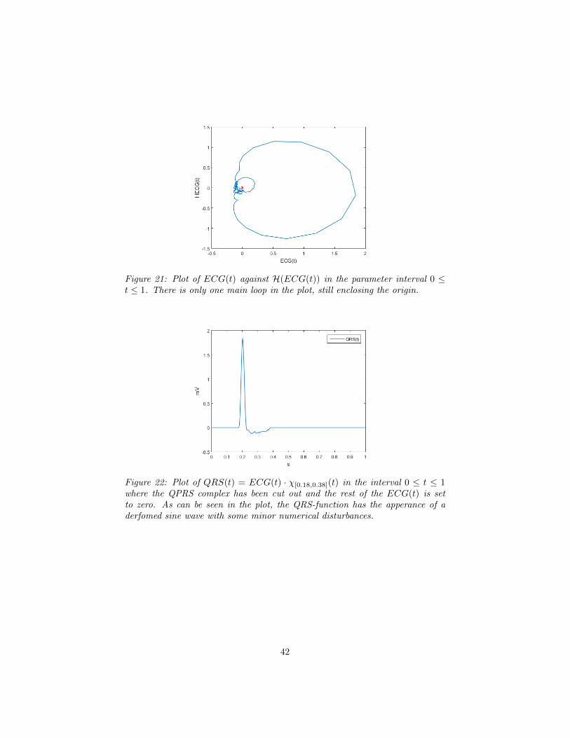
Figure 21: Plot of ECG(t) against H(ECG(t)) in the parameter interval 0 ≤t ≤ 1. There is only one main loop in the plot, still enclosing the origin.
Figure 22: Plot of QRS(t) = ECG(t) · χ[0.18,0.38](t) in the interval 0 ≤ t ≤ 1where the QPRS complex has been cut out and the rest of the ECG(t) is setto zero. As can be seen in the plot, the QRS-function has the apperance of aderfomed sine wave with some minor numerical disturbances.
42

Figure 23: Plot of QRS(t) against H(QRS(t)) in the parameter interval 0 ≤t ≤ 1. The only thing visible in the plot is a large main loop. This means thatthe analytic expansion of QRS(t) itself corresponds to a main loop enclosing theorigin.
Figure 24: A plot over the error∣∣H (QRS(t)) +H (r(t))−H
(ECG(t) · χ[0,1]
)∣∣.Since the error is very small, the numerical Hilbert transform exhibits linearity.
2.4 Limitation of the method
When does this method not work for detection of the QRS complex? Considersome other ECG-signal, ECG(t), as in Figure 25. The difference here is thatthe altitude of the QRS complex is considerably lower. As before,we expandECG(t) into an analyhtic signal
z(t) = ECG(t) + iH(ECG(t))
43

and in Figure 26 there is a plot of ECG(t) against H(ECG(t)). In this plotwe see that there is not one distinguishable main loop anymore. Therefore, thealgorithm will possibly fail to detect the QRS complex or the T-wave will beinterpreted as an QRS complex.
To conclude, for the method to work the height QRS complex needs to bedistinguishably higher than the rest of the ECG-signal.
Figure 25: A slightly modified ECG-signal with a considerably lower QRS com-plex.
Figure 26: A slightly modified ECG-signal with a considerably lower QRS com-plex.
44

3 The Hilbert-Huang transform
A time series is a collection of data points for a fluctuating variable that hasbeen sampled sequentially in time. We will denote a time series by X(t) whichsimply denotes the value of the time series at a time t. The time series thatwill be considered here will be continuous ones, meaning that they have beensampled continuously in time [5] .
There are several types of tools available to analyze a time series, most fa-mously is perhaps the Fourier transform. However, if the data in question comesfrom a nonstationary or nonlinear process there are limitations and the Fouriertransform may not be a suitable tool. For these time series the Hilbert-Huangtransform (HHT) is useful. The method is developed entirely in an empericalsense and is lacking an underlying mathematical framework.
Before presenting the method and an algorithm to carry out said method weneed, however, a definition and the introduction of some new concepts [5].
Definition 3.1. (IMF). An Intrinsic Mode Function (IMF) is a continous,real-valued function that satisfies the following two conditions
(i) The number of local extrema and zero crossings must be equal or differby most one
(ii) The mean value of the two envelopes curves formed by the extremas(local minima and maxima, respectively) should be zero at any time
Remark 3.2. Certainly, it begs the question, what is the ”envelope formed bythe extremas”? This is simply some smooth curve connecting the local maximaor local minima respectively. An envelope curve for the maxima is called eu(t)and for the minima el(t). Usually, cubic spline interpolation is used to constructthese two envelope curves.
The approach and idea of HHT is based on Emperical Mode Decomposition(EMD) where the time series is decomposed into IMFs. The extraction of anIMF from a time series is refered to as sifting. Each IMF will represent anintrinsic oscillation that is present in said time series [5], [17], [16].
3.1 An algorithm for decomposition
Consider a continuous time series X(t). An algorithm to carry out an EMD forthe time series is as follows. Let h10 = X(t).
(i) Locate each local maximum of X(t) and construct an envelope curve con-necting all maxima using cubic spline interpolation.
45

(ii) Locate each local minimum of X(t) and construct an envelope curve con-necting all minimas using cubic spline interpolation.
(iii) Construct a mean curve of these two envelope curves and call it m11(t).The first index refers to the particular IMF under construction and thesecond index tells us which iteration (extracting one IMF may requireseveral iterations) we are in for said IMF.
(iv) Calculate h11(t) = h10(t)−m11(t) = X(t)−m11(t). This should be closeto an IMF but it may need some refinement.
(v) Treat h11(t) as input data and repeat steps (i), (ii) and (iii) with h12(t) =h11(t)−m12(t).
(vi) Repeat k times with an appropriate stopping criterion finally ending upwith h1k(t) = h1(k−1)(t)−m1k(t).
(vii) Finally h1k(t) is subtracted from X(t) to give h20(t). Process then restartswith the dataset h20(t).
(viii) Set ci(t) = hik(t).
For step (vi) we need a stopping criterion. The most commonly used criterionis by looking at the sum of the difference, SD, derived from two consecutiveiterations. That is, hn(k−1)(t) and hnk(t) [10]. Also, since the algorithm iscarried out numerically, suppose the time series is in a finite time interval,0 ≤ t ≤ T .
SDn =
T∑t=0
(|hn(k−1)(t)− hnk(t)|2
h2n(k−1)(t)
)Empirically derived, an appropriate stopping criterion is then given by SDn < εwhere ε is some number between 0.2 and 0.3. But when should the overall siftingprocess stop? We may calculate
rn(t) = X(t)−n∑i=1
ci(t)
where rn(t) is a residual term. Naturally, when rn(t) has become monotonicor constant, no more IMFs may be extracted from X(t) and the sifting shouldbe stopped. Therefore, when rn(t) is either monotonic or constant the siftingprocess is complete. The final decomposition of X(t) has thus been obtainedand is obviously given by the expression
X(t) =
n∑i=1
ci(t) + rn(t)
where rn(t) is, again, a residual term. Since rn(t) is either monotonic or constant[10] one of the useful properties of the HHT is that it seperates trends or meansfrom the harmonics of a time series. Thus, when examining a time series thereis no inherent requirement of removing linear trends or unwanted offsets.
46

Example 3.3. We will consider one step of this algorithm where the first IMF,c1(t), is extracted from a function X(t) which can be seen in Figure 27. Puth10(t) = X(t). In Figure 28 we see that m11(t), which is is the mean curve ofthe two envelope curves is not zero. Therefore, h10(t) is not an IMF itself andh11(t) = h10(t)−m11(t) is calculated.
Figure 27: Plot of function X(t) from which we will extract c1(t).
Figure 28: Plot of h10(t) with its envelope curves and mean curve.
Visibly, in Figure 29 we can see that h11(t) is much closer to an IMF comparedto h10(t) . In Figure 30 - 31 the above steps are repated in order to refine h11(t)and make it look like a true IMF.
47
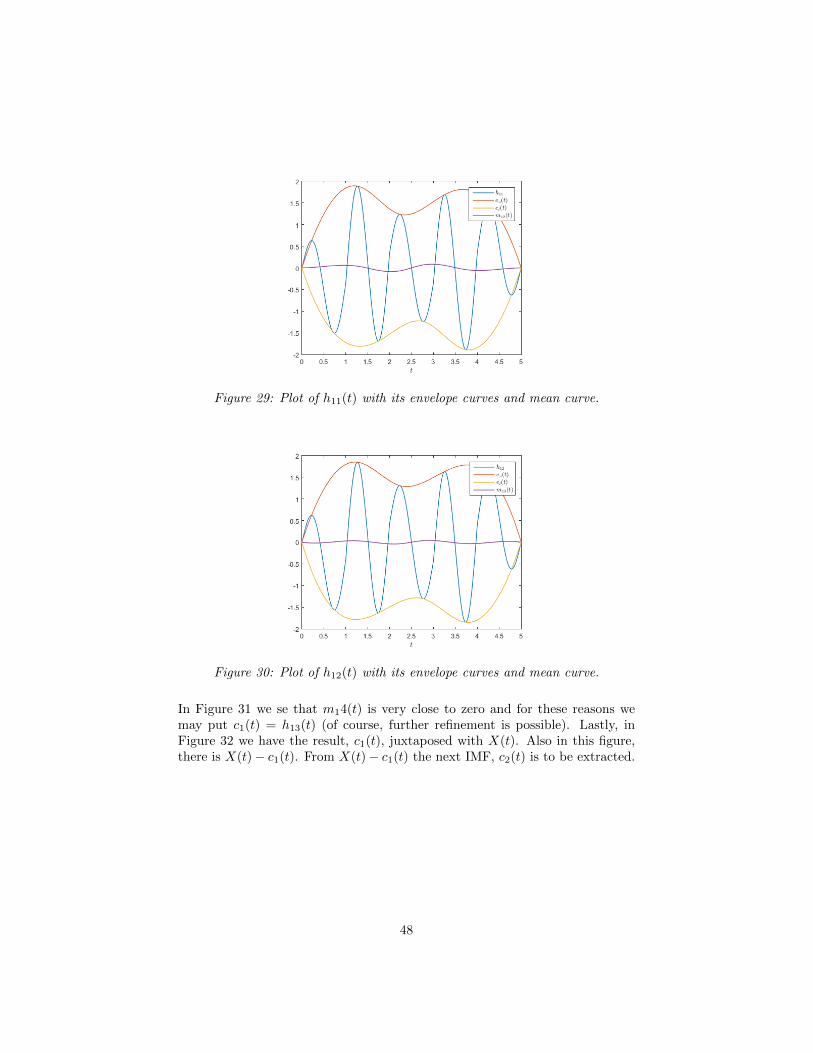
Figure 29: Plot of h11(t) with its envelope curves and mean curve.
Figure 30: Plot of h12(t) with its envelope curves and mean curve.
In Figure 31 we se that m14(t) is very close to zero and for these reasons wemay put c1(t) = h13(t) (of course, further refinement is possible). Lastly, inFigure 32 we have the result, c1(t), juxtaposed with X(t). Also in this figure,there is X(t)− c1(t). From X(t)− c1(t) the next IMF, c2(t) is to be extracted.
48
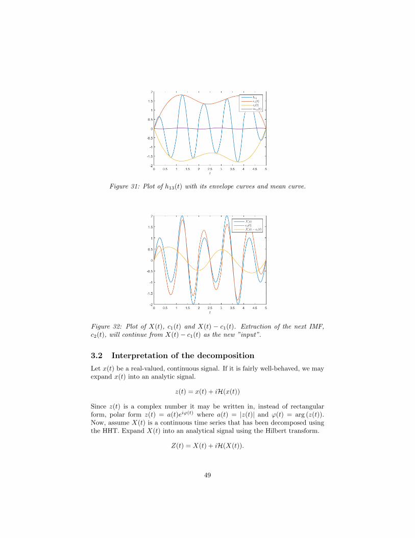
Figure 31: Plot of h13(t) with its envelope curves and mean curve.
Figure 32: Plot of X(t), c1(t) and X(t) − c1(t). Extraction of the next IMF,c2(t), will continue from X(t)− c1(t) as the new ”input”.
3.2 Interpretation of the decomposition
Let x(t) be a real-valued, continuous signal. If it is fairly well-behaved, we mayexpand x(t) into an analytic signal.
z(t) = x(t) + iH(x(t))
Since z(t) is a complex number it may be written in, instead of rectangularform, polar form z(t) = a(t)eiϕ(t) where a(t) = |z(t)| and ϕ(t) = arg (z(t)).Now, assume X(t) is a continuous time series that has been decomposed usingthe HHT. Expand X(t) into an analytical signal using the Hilbert transform.
Z(t) = X(t) + iH(X(t)).
49

Using the decomposition, we disregard the residual term, rn(t). Either rn(t) is aconstant and thenH(rn(t)) = H(r) = 0, or it is monotonic. If rn(t) is monotonicthen it can potentially overpower the harmonics and should therefore be left out.
Define ω(t) = ddtϕ(t) where ω(t) is angular frequency. From this definition it
also follows that ω(t) = 2πf(t) where f(t) is called frequency. Now, from theanalytical expansion of X(t) along with the decomposition of X(t) through HHTwe get
Z(t) =
n∑j=1
cj(t) + iH
n∑j=1
cj(t)
=
n∑j=1
(cj(t) + iHcj(t))
=
n∑j=1
aj(t)eiϕj(t) =
n∑j=1
aj(t)ei(ϕ(0)+
∫ t0ωj(s)ds)
=
n∑j=1
aj(t)eiϕ(0)+2πi
∫ t0fj(s)ds.
Thus, another way of representing the time series X(t) is given by
X(t) = Re (Z(t)) = Re
n∑j=1
aj(t)eiϕ(0)+2πi
∫ t0fj(s)ds
. (1)
Now, suppose that X(t) were to be expanded into a Fourier representation.Given in complex form, its Fourier representation would be
X(t) =
∞∑j=−∞
aje2πifjt. (2)
Obviously, these expressions are very similar but they differ in an very impor-tant aspect. In (2), the amplitudes, aj , and frequencies, fj , are constant whilethe corresponding terms are time dependent in (1). Thus, the HHT with itsdecomposition can be viewed as a generalized Fourier series expansion. Thetime varying amplitudes and frequencies allows for a better representation of anonstationary time series [5].
This new expression of a time series allows us to represent the amplitude andfrequncy as functions of time in a 3-D plot. Having a plane with a f - and t-axisthe amplitude may be contoured. This f -t-distibution of the amplitude is calledthe Hilbert spectrum and usually denoted as H(f, t). Also, with H(f, t) definedit makes sense to also define the marginal spectrum, h(f), which is given by
h(f) =
∫ T
0
H(f, t)dt.
50

The marginal spectrum can, in some sense, be compared with the amplitudespectrum of a Fourier representation of X(t) given by |X(f)| in the frequencydomain. However, there is one important distinction that one has to keep inmind. For the Fourier representation, if |X(f)| 6= 0 for a certain f , this meansthat a harmonic with the same frequency persisted throughout the whole timeseries. If h(f) 6= 0 for the very same frequency f , it merely means that thereis a higher likelihood for such a harmonic to have existed locally somehwere inthe distribution. The exact time of occurence of this harmonic is provided bythe complete Hilbert spectrum [10], [15].
Example 3.4. Consider the function
X(t) =
sin (t2) + t, 0 ≤ t ≤ 25
sin (20πt) + t, 25 ≤ t ≤ 100.
In this function there is a chirp where the frequency increases linearly in time.That is, f(t) = f0 + kt and the chirp signal is sin (f(t) · t) (in our case, f0 = 0and k = 1). Also, there is also a linear trend present in the function. Clearly,the process represented by the given function is non-linear and nonstationary.Using methods from Fourier analysis to analyze this function is therefore nota good idea since the linear trend will dominate. Using detrend in MATLABremoves the linear trend and in Figure Figure 33 we have the amplitude spec-trum, |X(f)|, of X(t). While the frequency components we expect are present,the Fourier transform does not tell us when the two different harmonics occur.We may, however, use the HHT to demcompose X(t) into IMFs using the HHT.With the decomposition, a Hilbert spectrum may be plotted. In Figure 34 aHilbert spectrum for X(t) can be seen.
From this spectrum it is easy to see that in the interval 0 ≤ t ≤ 25 the fre-quency of the harmonics are given by 1
2π ·f(t) = t2π . Furthermore, in the interval
25 ≤ t ≤ 100 the frequency of the harmonics are given by f = 20π/(2π) = 10and this also clearly reflected by the Hilbert spectrum.
51

Figure 33: Amplitude spectrum of a ”detrended” version of X(t). This spectrumconceived by Fourier methods does not reflect that we have a chirp signal andthat X(t) is nonstationary.
Figure 34: Hilbert spectrum of X(t).
In this section some various numerical investigations of the HHT will be carriedout. This is an attempt to try to deduce some properties of the transform in anempirical manner. Also, what weaknesses are inherit in the method?
By looking at the HHT algorithm (or empirical investigation) it is clear thatthe IMFs given by ck(t), 1 ≤ k ≤ n decreases in complexity as k increases. Thehigher complexity of an IMF (more zero crossings and extremas) the higher isits frequency content. Therefore, the following conjecture makes sense.
52

Conjecture 3.5. SupposeX(t) is a time series and its Hilbert-Huang trans-form is a decomposition given by
X(t) =
n∑i=1
ci(t) + rn(t).
Then the IMFs, ck(t), are decreasing in complexity as k increases. Thatis, given ck(t) and ck+1(t), then ck(t) has more zero crossings compared tock+1(t) for 1 ≤ k ≤ n− 1.
The validity of this conjecture will be investigated throughout the thesis. Notethat more zero crossing means that ck(t) has higher frequency content comparedto ck+1(t).
3.3 Trigonometric polynomials and the HHT
Definition 3.6. A function f(t) is said to be a trigonometric polynomialof degree N if it can be written in the form
X(t) = a0 +
N∑n=1
an cos (nt) +
N∑n=1
bn sin (nt)
where an, bk for 1 ≤ n ≤ N are any complex numbers.
It is easy to see that an cos (nt) and bn sin (nt) for any fix n will satisfy bothconditions (i) and (ii) from Definition 3.1. Therefore, an interesting observationis that a trigonometric polynomial is in fact a sum of several functions that eachone is an IMF, plus some constant a0. If given a function X(t) known to be atrigonometric polynomial, is it possible to decompose it using the HHT?
Example 3.7. Consider the function
X1(t) = 4 cos (10t) + 2 cos (t)
which is a very simple trigonometric polynomial consisting of only two com-ponents. As can be seen in a plot of the function in Figure 35 it is, despiteX1(t) being a fairly simple function, hard to determine what components X1(t)actually contains. To extract the different components from X1(t), the Hilbert-Huang Transform should prove useful.
When performing HHT on X1(t) we should, according to Conjecture 3.5,
53

Figure 35: Plot of X1(t) = 4 cos (10t) + 2 cos (t).
for the first IMF receive c1(t) = 4 cos (10t) since this is the component with thehighest frequency content in X1(t). Naturally, for the second IMF we expectto recieve c2(t) = 2 cos (t) which of course is the component in X2(t) with thesecond highest frequency content.
The results of performing the HHT numerically on X(t) can be seen in Figure 36.The results seem to be in line with our predictions and it looks very much likec1(t) = 4 cos (10t) and c2(t) = 2 cos (t) as expected. This can be seen moreclearly in Figure 37 where the differences c1(t)− 4 cos (10t) and c2(t)− 2 cos (t)are plotted. Except for some edge effects (which will be adressed later) it is clearthat the differences are virtually zero throughout the interval. To summarize,
Figure 36: Plot of c1(t) and c2(t) calculated numerically through the HHT algo-rithm for X1(t) for 0 ≤ t ≤ 25.
54

Figure 37: Plot of the difference between expected IMFs and the actual IMFscalculated through the HHT for 0 ≤ t ≤ 25.
the HHT worked as exepected on X1(t), both with regards to Conjecture 3.5and as a suitable tool for extracting the compononents of a trigonometric poly-nomial. Note that here is the residual term, r2(t), equal to zero because X1(t)consists completely of IMFs.
Remark 3.8. The interval 0 ≤ t ≤ 25 is arbitrary. One should note thatthe HHT performs better if the interval is larger. This is of course due tothe numerical algorithm having more data points to consider. The interval inquestion gives good result and thus will be used.
Example 3.9. Consider the function
X2(t) = cos (5t) + cos (t) + 3
which can be seen in Figure 38. What happens when a0 6= 0 for a trigonometricpolynomial in regards to the HHT? Obviously the constant a0 is not an IMFfunction since it does not satisfy condition (ii) in Definition 5.1. Therefore,the constant will end up in the residual term. In this case, we should getc1(t) = cos (5t), c2(t) = cos (t) and r2(t) = 3. Like in the first example, thisis empirically proven by calculating the HHT for X2(t) and the results can beseen in Figure 39 and Figure 40.
55

Figure 38: Plot of X2(t) = cos (5t) + cos (t) + 3.
Figure 39: Plot of c1(t), c2(t) and r2(t) calculated numerically through the HHTalgorithm for X2(t) .
56

Figure 40: Plot of the difference between expected IMF:s and the actual IMF:scalculated through the HHT.
3.4 Nonstationary processes and the HHT
One of the benefits of the HHT is that it can handle non-stationary time series.
Example 3.10. Consider the function
X3(t) =
sin (t), 0 ≤ t ≤ 4π
sin (3t), 4π ≤ t ≤ 20
which can be seen in Figure 41. Clearly, X3(t) is continuous everywhere andboth of the two seperate functions in each interval is an IMF and thus X3(t)itself is an IMF. Ideally, the Hilbert-Huang transform of X3(t) should simplyreturn X3(t) itself. This is also the case as can be seen in Figure 42 where c1(t)appears to be identical to X3(t). This is confirmed to be the case in the verysame figure. We see that the difference of c1(t) and X(t) is zero everywhere.Also, r1(t) is zero everywhere as should be expected.
57

Figure 41: Plot of X3(t).
Figure 42: Plot of c1(t) and the difference of c1(t) and X3(t).
Example 3.11. Consider the function
X4(t) =
sin (t), 0 ≤ t ≤ 10π
sin (t) + sin (10t), 10π ≤ t ≤ 100
which can be seen in Figure 43. Calculating the HHT for a function like thisand succesfully extracting and separating the harmonics could be very useful.Imagine we have some background process that is suddenly interrupted by an-other process (like an earthquake). While the ”new” process is dominating thebackground process is still active. Obviously, this is a nonstationary situationand therefore the HHT could be very useful in acquiring the harmonics.
58

Figure 43: Plot of X4(t).
According to Conjecture 3.5, the IMFs we should expect are
c1(t) =
sin (t), 0 ≤ t ≤ 10π
sin (10t), 10π ≤ t ≤ 100
c2(t) =
0, 0 ≤ t ≤ 10π
sin (t), 10π ≤ t ≤ 100
where the component with the highest frequency in each interval. The actualIMFs, acquired by calculation and denoted by c1(t) and c2(t) can be seen inFigure 44. Furthermore, in Figure 45 are the differences of the calculated IMFsand the expected IMFs.
What conclusions can be drawn? Obviously, c1(t) agrees well with c1(t) ex-cept for edge effects and in the neighborhood of t = 10π. Of course, this isbecause the harmonics shift instantaneously and it is hard for the algorithm tofit this in with IMFs. Despite this, the result of c1(t) should be considered goodsince it manages to pick up both harmonics in each interval. For c2(t), we donot really get what we expected. While it picks up the background harmonicsof sin (t) in 10π ≤ t ≤ 100, it is a bit off in 0 ≤ t ≤ 10π. This is because itis hard to fit an IMF to c2(t) which has a zero interval and then instantaneousharmonics.
59

Figure 44: Plot of the two first IMFs, calculated numerically for X4(t).
Figure 45: Plot of the difference between the calculated IMFs and the expectedIMFs for X4(t). That is, c1(t)− c1(t) and c2(t)− c2(t)
.
3.5 Limitations of HHT
As have been seen in the examples, there are some limitations inherent in theHHT. These limitations are due to the algorithm being carried out numericallyand because the data sets are indeed finite in the number of elements.
3.5.1 End effects
Comparing the difference between the expected IMF and the IMF calculatednumerically it has been clear that the difference can relatively large at the endpoints. This effect may be seen very clearly in Figure 37 for example. Expected
60

IMF and the IMF yielded by the algorithm correspond very well everywhere inthe interval except at the end point.
This unwanted effect is due to the datasets being of finite numbers of elements.Therefore, both end points of the data set only have one (instead of two) neigh-boring point to be considered. Unfortunately, these end effects will becomeamplified as for every IMF being calculated these effects will spread down tothe next and less complex IMF to be considered.
3.5.2 Adjacent frequencies
To discuss this limitation of the HHT, we will look at a concrete example.
Example 3.12. Consider the functions
X(t) = cos (10t) + cos (t)
Y (t) = cos (2t) + cos (t)
which can be seen in Figure 46. Both functions are simple trigonometric poly-nomials. Using the HHT to extract the components from each function shouldtherefore be fairly straightforward. In Figure 47 the two first IMFs for X(t)and Y (t) can be seen. For X(t) we have cX1 (t), cX2 (t) and for Y (t), in the samemanner, cY1 (t), cY2 (t) as the numerically calculated IMFs through the HHT.
Apart from the edge effects it is clear that the HHT algorithm provides goodresults for decomposing X(t). For X(t), the numerically calculated IMFs areclose to the expected IMFs. That is, cX1 (t)−cos (10t) and cX1 (t)−cos (t) are zeroor close to zero throughout the whole interval which can be seen in Figure 49.To conclude, the HHT works very well for X(t) and it manages to decomposethe harmonic components of this function.
Now, despite X(t) and Y (t) being very similar functions, the performance of theHHT is very different for Y (t). In Figure 50 it is clear that that the numericallycalculated IMFs are not close to the expected IMFs. That is, cY1 (t)− cos (2t) aswell as cY2 (t) − cos (t) are not close to zero throughout the interval. Quite thecontrary, both differences osciallate between fairly large numbers. To conclude,the HHT actually seems to perform quite badly for Y (t).
Question is, why is there such a difference in the performance of the HHT be-tween X(t) and Y (t)? The answer is obtained by looking at and comparing thefrequency components of X(t) and Y (t), respectively. Considering the Fouriertransform of X(t) we see that it contains fX = 10
2π ,12π (note that these are
separated by a factor 10). The same reasoning for Y (t) provides the frequencycomponents fY = 2
2π ,12π . Note that for Y (t) the different frequency components
are closer to each other, almost ajdacent. This becomes even clearer by looking
61

at the actual Fourier transforms of X(t) and Y (t) [6].
X(f) =1
2
(δ
(f − 10
2π
)+ δ
(f +
10
2π
))+
1
2
(δ
(f − 1
2π
)+ δ
(f +
1
2π
))Y (f) =
1
2
(δ
(f − 2
2π
)+ δ
(f +
2
2π
))+
1
2
(δ
(f − 1
2π
)+ δ
(f +
1
2π
))Analytically, the frequency components are well-separeted by the distinct Diracdelta functions. However, in a numerical representation these Dirac deltas func-tions will look like ”hills” in the frequency domain. This can be seen in Figure 50where |X(f)| = |F(X(t))| and |Y (f)| = |F(Y (t))| have been calculated numer-ically and plotted in the frequency domain. If these hills are too close to eachother, the algorithm will have trouble to differ between the two different fre-quency components. As a result, we will not receieve as neat and clear-cut IMFsfor Y (t) compared to X(t) and the numerical errors will increase if frequenciesare adjacent and too alike.
Figure 46: Plots of X(t) = cos (10t) + cos (t) and Y (t) = cos (2t) + cos (t).
62

Figure 47: Plots of the IMFs for X(t) and Y (t). The first plots shows the IMFsfor X(t) which are cX1 (t) and cX2 (t). The second plot shows the IMFs for Y (t)which are cY1 (t) and cY2 (t).
Figure 48: Plot of cX1 (t) − cos (10t) and cX2 (t) − cos (t). As can be seen in theplot, the expected IMFs are close to the calculated IMFs.
63

Figure 49: Plot of cY1 (t)−cos (2t) and cY2 (t)−cos (t). Visibly, the expected IMFsare not close to the calculated IMFs.
Figure 50: Plot of the power spectrums, |X(f)| and |Y (f)| for f ≥ 0 (note thatthe power spectrums are symmetric, since the signals in the time domain arereal). For |X(f)| we expect peaks at f = 1
2π ≈ 0.16 and f = 102π ≈ 1.60. For
Y (f) we expect peaks at f = 12π ≈ 0.16 and f = 2
2π ≈ 0.32. Looking at thepower spectrums, this is also the case.
Example 3.13. For a more quantative approach to the limitation of ajdacentfrequencies, consider the function
X(t, ε) = cos ((1 + ε)t) + cos (t)
for some ε > 0. How well does the HHT perform for different values of ε? Ideally,when X(t) is subject to HHT, the IMFs we expect are c1(t, ε) = cos ((1 + ε)t)and c2(t) = cos (t). To determine how well HHT performs for different values
64

of ε, let us calculate ‖c1(t, ε) − c1(t, ε)‖2 and ‖c2(t, ε) − c2(t)‖2 where c1(t, ε)and c2(t, ε) are the numerically calcuated IMFs for X(t, ε). The result can beseen in Figure 51 where 0.1 ≤ ε ≤ 30 with a step length of ∆ε = 0.1. Thefrequency components of X(t) are f = 1+ε
2π = 12π + ε
2π and f = 12π . Obviously,
as ε increases, the frequencies moves farther away from one another. Thus, theHHT experiences less problems of differentiating the two frequencies and theresults are better. In contrast, when ε is small, the frequencies are adjacaentand the results are bad as can be seen in said figure.
Figure 51: Plot of ‖c1(t, ε)− c1(t, ε)‖2 and ‖c2(t, ε)− c2(t)‖2 for 0.1 ≤ ε ≤ 30.
For reasonable results with the HHT, frequencies should be seperated by a factor5 to avoid problems with adjacency. For good results, a factor 10 is desirable.
65

4 Hilbert transform and modulation
4.1 Introduction to Amplitude modulation
Consider a purely real and continous signal m(t) that we want to transmit.Suppose its Fourier transform, M(f), is bandlimited (M(f) = 0 if |f | > W forsome W ) and also M(0) = 0. Usually when transmitting signals it is desiredthat they are within a given frequency band to avoid interference from othertransmissions. To achieve this property amplitude modulation may be used. Astandard amplitude modulated signal is given by
mAM (t) = m(t) cos (2πfct)
where fc is called the carrier frequency. The carrier frequency is much largerthan the bandwidth of m(t), that is, fc W [8]. Given the Fourier transform
Figure 52: Plot of |M(f)|, the amplitude spectrum of M(f). The symmetry isbecause m(t) is a real signal.
M(f) of m(t), the Fourier transform of mAM (t) is then given by
MAM (f) = F (mAM (t)) = F (m(t) cos (2πfct)) = F(m(t)) ∗ F(cos (2πfct)
= M(f) ∗ 1
2(δ(f − fc) + δ(f + fc)) =
1
2(M(f − fc) +M(f + fc))
As can be seen in the expression above, the effect cos (2πfct) has on the messagesignal m(t) is that it moves the frequency content of M(f) to fc and −fc. Thus,MAM (f) has ended up within a more desirable frequency which is around thecarrier frequency. One should note that M(f) is symetrically doubled aroundthe origin and each copy of M(f) is centered around fc and −fc rescpectivelyin MAM (f). Thus, the bandwidth used in MAM (f) is doubled compared tothe original message. One way to refine this method and to avoid the doublingin bandwidth is to use the method of Single-Sideband modulation (SSB). Thismethod makes use of the Hilbert transform and analytic signals and will beinvestigated further later.
Suppose that mAM (t) has been transmitted and received. How is the orignalmessage signal, m(t), extracted by the receiver? By simply multiplying with
66
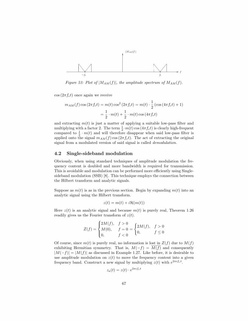
Figure 53: Plot of |MAM (f)|, the amplitude spectrum of MAM (f).
cos (2πfct) once again we receive
mAM (f) cos (2πfct) = m(t) cos2 (2πfct) = m(t) · 1
2(cos (4πfct) + 1)
=1
2·m(t) +
1
2·m(t) cos (4πfct)
and extracting m(t) is just a matter of applying a suitable low-pass filter andmultiplying with a factor 2. The term 1
2 ·m(t) cos (4πfct) is clearly high-frequentcompared to 1
2 ·m(t) and will therefore disappear when said low-pass filter isapplied onto the signal mAM (f) cos (2πfct). The act of extracting the originalsignal from a modulated version of said signal is called demodulation.
4.2 Single-sideband modulation
Obviously, when using standard techniques of amplitude modulation the fre-quency content is doubled and more bandwidth is required for transmission.This is avoidable and modulation can be performed more efficiently using Single-sideband modulation (SSB) [8]. This technique employs the connection betweenthe Hilbert transform and analytic signals.
Suppose as m(t) is as in the previous section. Begin by expanding m(t) into ananalytic signal using the Hilbert transform.
z(t) = m(t) + iH(m(t))
Here z(t) is an analytic signal and because m(t) is purely real, Theorem 1.26readily gives us the Fourier transform of z(t).
Z(f) =
2M(f), f > 0
M(0), f = 0
0, f < 0
=
2M(f), f > 0
0, f ≤ 0
Of course, since m(t) is purely real, no information is lost in Z(f) due to M(f)exhibiting Hermitian symmetry. That is, M(−f) = M(f) and consequently|M(−f)| = |M(f)| as discussed in Example 1.27. Like before, it is desirable touse amplitude modulation on z(t) to move the frequency content into a givenfrequency band. Construct a new signal by multiplying z(t) with e2πifct.
za(t) = z(t) · e2πifct
67

The Fourier transform of za(t) is easily calculated using convolution.
Za(f) = F(za(t)) = F(z(t) · e2πifct
)= F(z(t)) ∗ F
(e2πifct
)= Z(f) ∗ δ(f − fc) = Z(f − fc)
Using the derived expression for Z(f) from above we get the expression
Za(f) = Z(f − fc) =
2M(f − fc), f > fc
0, f ≤ fc
and accordingly it has both only positive frequency components and due to am-plitude modulation, said components lie about f = fc. Since all analytic signalshave only positive frequency components, za(t) is an analytic represenation ofan SSB-signal that we define as mSSB(t).
za(t) = mSSB(t) + iH(mSSB(t))
But we also have that
za(t) =z(t) · e2πifct = (m(t) + iH(m(t))) · (cos (2πfct) + i sin (2πfct))
=m(t) · cos (2πfct)−H(m(t)) · sin (2πfct) + i · [m(t) · sin (2πfct)+
+H(m(t)) · cos (2πfct)]
Since mSSB(t) = Re za(t) we get by simply identifying real parts
mSSB(t) = m(t) · cos (2πfct)−H(m(t)) · sin (2πfct)
By using Theorem 1.12 we can acquire the Fourier transform of mSSB(t).
MSSB(f) = F(mSSB(t)) = F(m(t) · cos (2πfct)−H(m(t)) · sin (2πfct))
= F(m(t)) ∗ F(cos (2πfct))−F(H(m(t))) ∗ F(sin (2πfct))
= M(f) ∗ 1
2(δ(f − fc) + δ(f + fc))−
− (−i sgn (f))M(f) ∗ 1
2i(δ(f − fc)− δ(f + fc))
=1
2(1 + sgn (f − fc))M(f − fc) +
1
2(1− sgn (f + fc))M(f + fc)
=
M(f − fc), f > fc
0, −fc ≤ f ≤ fcM(f + fc), f < −fc
From this we can draw the conclusion that the frequency content for the SSBhas been halved compared to the amplitude modulated signal. Demodulation,recovering m(t) from mSSB(t) that is, works in a similar fashion as before -
68
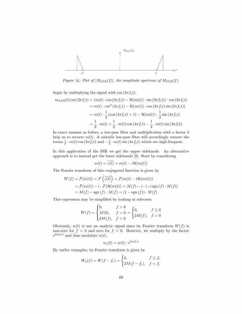
Figure 54: Plot of |MSSB(f)|, the amplitude spectrum of MSSB(f).
begin by multiplying the signal with cos (2πfct).
mSSB(t) cos (2πfct) = (m(t) · cos (2πfct)−H(m(t)) · sin (2πfct)) · cos (2πfct)
= m(t) · cos2 (2πfct)−H(m(t)) · cos (2πfct) sin (2πfct))
= m(t) · 1
2(cos (4πfct) + 1)−H(m(t)) · 1
2sin (4πfct)
=1
2·m(t) +
1
2·m(t) cos (4πfct)−
1
2·m(t) sin (4πfct)
In exact manner as before, a low-pass filter and multiplication with a factor 2help us to recover m(t). A suitable low-pass filter will accordingly remove theterms 1
2 ·m(t) cos (4πfct) and − 12 ·m(t) sin (4πfct) which are high-frequent.
In this application of the SSB we get the upper sidebands. An alternativeapproach is to instead get the lower sidebands [8]. Start by considering
w(t) = z(t) = m(t)− iH(m(t))
The Fourier transform of this conjugated function is given by
W (f) = F(w(t)) = F(z(t)
)= F(m(t)− iH(m(t)))
= F(m(t))− i · F(H(m(t)) = M(f)− i · (−i sgn (f) ·M(f))
= M(f)− sgn (f) ·M(f) = (1− sgn (f)) ·M(f)
This expression may be simplified by looking at subcases.
W (f) =
0, f > 0
M(0), f = 0
2M(f), f < 0
=
0, f ≥ 0
2M(f), f < 0
Obviously, w(t) is not an analytic signal since its Fourier transform W (f) isnon-zero for f < 0 and zero for f > 0. However, we multiply by the factore2πifct and thus modulate w(t).
wa(t) = w(t) · e2πifct
By earlier examples, its Fourier transform is given by
Wa(f) = W (f − fc) =
0, f ≥ fc2M(f − fc), f < fc
69

and if fc is large enough it is possible that Wa(f) = 0 for all f ≤ 0. How largedoes fc have to be? For f = 0 we have that Wa(0) = 2M(−fc) and becauseit is necessary that Wa(f) = 0 for all f ≤ 0 we must have that −fc < −Wwhich means that fc > W. If this is the case, wa(t) is an analytic signal sinceWa(f) = 0 for all f ≤ 0. Also, note that it is the lower sideband of M(f) in theexpression belonging to Wa(f). Consequently, it makes sense to put
wa(t) = mLSB(t) + iH(mLSB(t))
but as before we also have that
wa(t) =w(t) · e2πifct = (m(t)− iH(m(t))) · (cos (2πfct) + i sin (2πfct))
=m(t) · cos (2πfct) +H(m(t)) · sin (2πfct) + i · [m(t) · sin (2πfct)+
−H(m(t)) · cos (2πfct)]
Since mLSB(t) = Rewa(t) we get, once again, by simply identifying real parts
mLSB(t) = m(t) · cos (2πfct) +H(m(t)) · sin (2πfct)
and the Fourier transform of mLSB(t) is given by
MLSB(f) = F(mLSB(t)) = F(m(t) · cos (2πfct) +H(m(t)) · sin (2πfct))
= F(m(t)) ∗ F(cos (2πfct)) + F(H(m(t))) ∗ F(sin (2πfct))
= M(f) ∗ 1
2(δ(f − fc) + δ(f + fc)) +
+ (−i sgn (f))M(f) ∗ 1
2i(δ(f − fc)− δ(f + fc))
=1
2(1− sgn (f − fc))M(f − fc) +
1
2(1 + sgn (f + fc))M(f + fc)
=
M(f + fc), f > fc
M(f − fc) +M(f + fc), −fc ≤ f ≤ fcM(f − fc), f < −fc
however, since M(f + fc) = 0 for f > fc and M(f − fc) = 0 for f < −fc theexpression above may be further simplified.
MLSB(f) =
0, f > fc
M(f − fc) +M(f + fc), −fc ≤ f ≤ fc0, f < −fc
Clearly, in MLSB(f) only the lower sidebands are present as opposed to theexpression of MSSB(f) where we had the upper sidebands. Both methods havethe advantage of halving the required bandwidth for transmission and receivingtheir respective signals in the time domain.
70

Figure 55: Plot of |MLSB(f)|, the amplitude spectrum of MLSB(f).
71

5 Discussion
From the results presented in this thesis some conclusions may be drawn. Ofcourse, the discussion is focused around the Electrocardiagram and the Hilbert-Huang transform for which original research has been carried out.
5.1 Electrocardiogram
Provided an ECG-signal, ECG(t), and expanding this real valued signal intoan analytic signal given by
z(t) = ECG(t) + iH(ECG(t))
has proven to be an effective way of detecting the QRS complex. Since theQRS resembles a deformed sine wave, the parametric plot of z(t) will produce adistinguishable main loop in the complex plan if there is a QRS complex withinthe parametric interval. This main loop encloses the origin and therefore crossesall the axes.
The main reason that the method suggested to extract QRS complex in anECG signal lacks mathematical theory is because it does not work for all possi-ble ECG-signals. As was seen in the example in section 2.4, if the QRS complexis not high enough, the method does not work. This is because the lower QRScomplex does not produce any distinguishably large main loop in the paramet-ric plot of z(t). Depending on how the algorithm is constructed, either it willfail to detect the QRS complex or a T-wave may be misinterpreted as in theparametric plot and thus the detection of the QRS complex fails or a T-wave isincorrectly interpreted as a QRS complex.
The possibilities to expand this research is to prove the method mathemati-cally as opposed to numerical justifications (given one consider the limitationsmentioned above). Also, find ways for QRS complex detection to work beyondthe mentioned limitation.
5.2 Hilbert-Huang transform
The Hilbert-Huang transform (HHT) is a tool for analyzing time series that hasproven very effective. However, even though the method is gaining popularityit is still questionable why ”Fourier methods” still dominate spectral analysis.The HHT is a more versatile tool and has the ability to treat frequencies andamplitude as dependent on time. Thus, the HHT is very appropriate in ana-lyzing nonstationary and nonlinear time series in contrast to, for example, theFast Fourier Transform (FFT). One could easily argue that the HHT should bethe standard method for analyzing time series since stationarity and linearity isquite rare in real examples [10].
The HHT lacks mathematical theory because the empirical conceived method
72

does not work for all cases either. As seen in example 3.11, the algorithm failswhen frequencies are too cloose to each other (ajdacent frequencies).
The limitations of the HHT discovered during the experiments must be con-sidered. One possibility of further research in this area is how to further reducethese limitations - especially in the case of ”adjacent frequencies”. Possibly thealgorithm of decomposing could be refined to better deal with adjacent frequen-cies. Also, reducing, or even removing, the apparent end effects would of coursebe desirable.
The biggest advantage of the HHT is that it handles nonstationary processes sowell. For example, considering a scenario where we are measuring seismic wavesin connection with earthquake activity. Because of the nonstationary natureof these situations, as the frequency of the seismic waves fluctuate with time,the HHT is a very appropriate tool in analyzing these waves. In these types ofsituations, a Fourier spectral analysis oftentimes not suitable.
73

References
[1] Werner, J., Krantz, M., EKG, Bokakademin, Linkoping, 2003.
[2] Abeysekera, R.M.S.S., Bolton, R.J., Westphal, L.C. and Boashash, B., Pat-terns in Hilbert Transforms and Wigner-Wille Distributions of Electrocar-diogram Data, IEEE International Conference on ICASSP, 11 (1986), 1973-1978.
[3] European ST-T Database, 2000.Available online at http://physionet.org/physiobank/database/edb/.
[4] King, F.W., Hilbert Transforms Volume 1, Cambridge University Press,Cambridge, 2009.
[5] King, F.W., Hilbert Transforms Volume 2, Cambridge University Press,Cambridge, 2009.
[6] Hahn, S., Hilbert transforms in signal processing, Artech House, Inc., Nor-wood, 1996.
[7] Aigner, M., Fourieranalys, Bokakademin, Linkoping, 2015.
[8] Olofsson, M., Signal theory, Studentlitteratur, Lund, 2011.
[9] Alexandersson, L., TATA45 Komplex analys, Bokakademin, Linkoping,2014.
[10] Huang, N.E., et al, The empirical mode decomposition and the Hilbertspectrum for nonlinear and non-stationary time series analysis, The RoyalSociety, 454 (1998), 903-995.
[11] Kreyszig, E., Introductory Functional Analysis with Applications, John Wi-ley & Sons Inc, Windsor, 1978.
[12] Alavi-Sereshki, M.M., Analytical signals and Hilbert transforms, Texas TechUniversity, Lubbock, 1972.
[13] Benitez, D., et al., The use of the Hilbert transform in ECG signal analysis,Computers in Biology and Medicine, 31 (2001), 399–406.
[14] Linderhed, A., Adaptive image compression with wavelet packets and empir-ical mode decomposition, Linkoping University Post Print, Linkoping, 2004.
[15] Sahoo, J.P., Analysis of ECG signal for Detection of Cardiac Arrhythmias,National Institute Of Technology Rourkela, Orissa, 2011.
[16] Tolwinski, S., The Hilbert Transform and Empirical Mode Decompositionas Tools for Data Analysis, University of Arizona, Tuscon, 2007.
[17] Gong, K., Speech processing using the empirical mode decomposition andthe Hilbert transform, Concordia University, Montreal, 2004.
74

[18] Tan, A., Hilbert-Huang Transform algorithm for MATLAB, 2008.Available online at http://goo.gl/Fejjvy.
[19] Huang, N.E., Hilbert-Huang Transform And Its Applications, World Scien-tific Publishing Co Pte Ltd, Singapore, 2005.
75

Copyright
The publishers will keep this document online on the Internet - or its possi-ble replacement - for a period of 25 years from the date of publication barringexceptional circumstances. The online availability of the document implies apermanent permission for anyone to read, to download, to print out single copiesfor your own use and to use it unchanged for any non-commercial research andeducational purpose. Subsequent transfers of copyright cannot revoke this per-mission. All other uses of the document are conditional on the consent of thecopyright owner. The publisher has taken technical and administrative mea-sures to assure authenticity, security and accessibility. According to intellectualproperty law the author has the right to be mentioned when his/her work isaccessed as described above and to be protected against infringement. For ad-ditional information about the Linkoping University Electronic Press and itsprocedures for publication and for assurance of document integrity, please referto its WWW home page: http://www.ep.liu.se/
Upphovsratt
Detta dokument halls tillgangligt pa Internet – eller dess framtida ersattare –under 25 ar fran publiceringsdatum under forutsattning att inga extraordinaraomstandigheter uppstar. Tillgang till dokumentet innebar tillstand for var ochen att lasa, ladda ner, skriva ut enstaka kopior for enskilt bruk och att anvandadet oforandrat for ickekommersiell forskning och for undervisning. Overforingav upphovsratten vid en senare tidpunkt kan inte upphava detta tillstand. Allannan anvandning av dokumentet kraver upphovsmannens medgivande. Foratt garantera aktheten, sakerheten och tillgangligheten finns det losningar avteknisk och administrativ art. Upphovsmannens ideella ratt innefattar rattatt bli namnd som upphovsman i den omfattning som god sed kraver vidanvandning av dokumentet pa ovan beskrivna satt samt skydd mot att doku-mentet andras eller presenteras i sadan form eller i sadant sammanhang som arkrankande for upphovsmannens litterara eller konstnarliga anseende eller ege-nart. For ytterligare information om Linkoping University Electronic Press seforlagets hemsida http://www.ep.liu.se/
c© 2015, Mans Klingspor
76


