1

History and Theoretical Basics of Hidden Markov Models

Guy Leonard Kouemou EADS Deutschland GmbH,

Germany

1. Introduction

The following chapter can be understood as one sort of brief introduction to the history and basics of the Hidden Markov Models. Hidden Markov Models (HMMs) are learnable finite stochastic automates. Nowadays, they are considered as a specific form of dynamic Bayesian networks. Dynamic Bayesian networks are based on the theory of Bayes (Bayes & Price, 1763). A Hidden Markov Model consists of two stochastic processes. The first stochastic process is a Markov chain that is characterized by states and transition probabilities. The states of the chain are externally not visible, therefore “hidden”. The second stochastic process produces emissions observable at each moment, depending on a state-dependent probability distribution. It is important to notice that the denomination “hidden” while defining a Hidden Markov Model is referred to the states of the Markov chain, not to the parameters of the model. The history of the HMMs consists of two parts. On the one hand there is the history of Markov process and Markov chains, and on the other hand there is the history of algorithms needed to develop Hidden Markov Models in order to solve problems in the modern applied sciences by using for example a computer or similar electronic devices.

1.1. Brief history of Markov process and Markov chains Andrey Andreyevich Markov (June 14, 1856 – July 20, 1922) was a Russian mathematician. He is best known for his work on the theory of stochastic Markov processes. His research area later became known as Markov process and Markov chains. Andrey Andreyevich Markov introduced the Markov chains in 1906 when he produced the first theoretical results for stochastic processes by using the term “chain” for the first time. In 1913 he calculated letter sequences of the Russian language. A generalization to countable infinite state spaces was given by Kolmogorov (1931). Markov chains are related to Brownian motion and the ergodic hypothesis, two topics in physics which were important in the early years of the twentieth century. But Markov appears to have pursued this out of a mathematical motivation, namely the extension of the law of large numbers to dependent events. Out of this approach grew a general statistical instrument, the so-called stochastic Markov process. In mathematics generally, probability theory and statistics particularly, a Markov process can be considered as a time-varying random phenomenon for which Markov properties are

www.intechopen.com

Hidden Markov Models, Theory and Applications

4

achieved. In a common description, a stochastic process with the Markov property, or memorylessness, is one for which conditions on the present state of the system, its future and past are independent (Markov1908),(Wikipedia1,2,3). Markov processes arise in probability and statistics in one of two ways. A stochastic process, defined via a separate argument, may be shown (mathematically) to have the Markov property and as a consequence to have the properties that can be deduced from this for all Markov processes. Of more practical importance is the use of the assumption that the Markov property holds for a certain random process in order to construct a stochastic model for that process. In modelling terms, assuming that the Markov property holds is one of a limited number of simple ways of introducing statistical dependence into a model for a stochastic process in such a way that allows the strength of dependence at different lags to decline as the lag increases. Often, the term Markov chain is used to mean a Markov process which has a discrete (finite or countable) state-space. Usually a Markov chain would be defined for a discrete set of times (i.e. a discrete-time Markov Chain) although some authors use the same terminology where "time" can take continuous values.

1.2 Brief history of algorithms need to develop Hidden Markov Models

With the strong development of computer sciences in the 1940's, after research results of scientist like John von Neuman, Turing, Conrad Zuse, the scientists all over the world tried to find algorithms solutions in order to solve many problems in real live by using deterministic automate as well as stochastic automate. Near the classical filter theory dominated by the linear filter theory, the non-linear and stochastic filter theory became more and more important. At the end of the 1950's and the 1960's we can notice in this category the domination of the "Luenberger-Observer", the "Wiener-Filter", the „Kalman-Filter" or the "Extended Kalman-Filter" as well as its derivatives (Foellinger1992), (Kalman1960). At the same period in the middle of the 20th century, Claude Shannon (1916 – 2001), an American mathematician and electronic engineer, introduced in his paper "A mathematical theory of communication'', first published in two parts in the July and October 1948 editions of the Bell System Technical Journal, a very important historical step, that boosted the need of implementation and integration of the deterministic as well as stochastic automate in computer and electrical devices. Further important elements in the History of Algorithm Development are also needed in order to create, apply or understand Hidden Markov Models: The expectation-maximization (EM) algorithm: The recent history of the expectation-maximization algorithm is related with history of the Maximum-likelihood at the beginning of the 20th century (Kouemou 2010, Wikipedia). R. A. Fisher strongly used to recommend, analyze and make the Maximum-likelihood popular between 1912 and 1922, although it had been used earlier by Gauss, Laplace, Thiele, and F. Y. Edgeworth. Several years later the EM algorithm was explained and given its name in a paper 1977 by Arthur Dempster, Nan Laird, and Donald Rubin in the Journal of the Royal Statistical Society. They pointed out that the method had been "proposed many times in special circumstances" by other authors, but the 1977 paper generalized the method and developed the theory behind it. An expectation-maximization (EM) algorithm is used in statistics for finding maximum likelihood estimates of parameters in probabilistic models, where the model depends on unobserved latent variables. EM alternates between performing an expectation (E) step, which computes an expectation of the likelihood by including the latent variables as if they

www.intechopen.com

History and Theoretical Basics of Hidden Markov Models

5

were observed, and maximization (M) step, which computes the maximum likelihood estimates of the parameters by maximizing the expected likelihood found on the E step. The parameters found on the M step are then used to begin another E step, and the process is repeated. EM is frequently used for data clustering in machine learning and computer vision. In natural language processing, two prominent instances of the algorithm are the Baum-Welch algorithm (also known as "forward-backward") and the inside-outside algorithm for unsupervised induction of probabilistic context-free grammars. Mathematical and algorithmic basics of Expectation Maximization algorithm, specifically for HMM-Applications, will be introduced in the following parts of this chapter. The Baum-Welch algorithm: The Baum–Welch algorithm is a particular case of a generalized expectation-maximization (GEM) algorithm (Kouemou 2010, Wikipedia). The Baum–Welch algorithm is used to find the unknown parameters of a hidden Markov model (HMM). It makes use of the forward-backward algorithm and is named for Leonard E. Baum and Lloyd R. Welch. One of the introducing papers for the Baum-Welch algorithm was presented 1970 "A maximization technique occurring in the statistical analysis of probabilistic functions of Markov chains", (Baum1970). Mathematical and algorithmic basics of the Baum-Welch algorithm specifically for HMM-Applications will be introduced in the following parts of this chapter. The Viterbi Algorithm: The Viterbi algorithm was conceived by Andrew Viterbi in 1967 as a decoding algorithm for convolution codes over noisy digital communication links. It is a dynamic programming algorithm (Kouemou 2010, Wikipedia). For finding the most likely sequence of hidden states, called the Viterbi path that results in a sequence of observed events. During the last years, this algorithm has found universal application in decoding the convolution codes, used for example in CDMA and GSM digital cellular, dial-up modems, satellite, deep-space communications, and 802.11 wireless LANs. It is now also commonly used in speech recognition applications, keyword spotting, computational linguistics, and bioinformatics. For example, in certain speech-to-text recognition devices, the acoustic signal is treated as the observed sequence of events, and a string of text is considered to be the "hidden cause" of the acoustic signal. The Viterbi algorithm finds the most likely string of text given the acoustic signal (Wikipedia, David Forney's). Mathematical and algorithmic basics of the Viterbi-Algorithm for HMM-Applications will be introduced in the following parts of this chapter. The chapter consists of the next following parts: • Part 2: Mathematical basics of Hidden Markov Models • Part 3: Basics of HMM in stochastic modelling • Part4: Types of Hidden Markov Models • Part5: Basics of HMM in signal processing applications • Part6: Conclusion and References

2. Mathematical basics of Hidden Markov Models

Definition of Hidden Markov Models

A Hidden Markov Model (cf. Figure 1) is a finite learnable stochastic automate. It can be summarized as a kind of double stochastic process with the two following aspects: • The first stochastic process is a finite set of states, where each of them is generally

associated with a multidimensional probability distribution. The transitions between

www.intechopen.com

Hidden Markov Models, Theory and Applications

6

the different states are statistically organized by a set of probabilities called transition probabilities.

• In the second stochastic process, in any state an event can be observed. Since we will just analyze what we observe without seeing at which states it occurred, the states are "hidden" to the observer, therefore the name "Hidden Markov Model".

Each Hidden Markov Model is defined by states, state probabilities, transition probabilities, emission probabilities and initial probabilities. In order to define an HMM completely, the following five Elements have to be defined: 1. The N states of the Model, defined by

{ }1 ,..., NS S S= (1)

2. The M observation symbols per state { }1 ,..., MV v v= . If the observations are continuous then M is infinite.

3. The State transition probability distribution { }ijA a= , where ija is the probability that the state at time 1t + is jS , is given when the state at time t is iS . The structure of this stochastic matrix defines the connection structure of the model. If a coefficient ija is zero, it will remain zero even through the training process, so there will never be a transition from state iS to

jS . { }1 | , 1 ,ij t ta p q j q i i j N+= = = ≤ ≤ (2)

Where tq denotes the current state. The transition probabilities should satisfy the

normal stochastic constraints, 0, 1 ,ija i j N≥ ≤ ≤ and1

1, 1N

ijj

a i N=

= ≤ ≤∑ .

4. The Observation symbol probability distribution in each state, { }( )jB b k= where ( )jb k is the probability that symbol kv is emitted in state jS .

{ }( ) | , 1 , 1j t k tb k p o v q j j N k M= = = ≤ ≤ ≤ ≤ (3)

where kv denotes the thk observation symbol in the alphabet, and to the current parameter vector. The following stochastic constraints must be satisfied:

( ) 0, 1 , 1jb k j N k M≥ ≤ ≤ ≤ ≤ and 1

( ) 1, 1M

jk

b k j N=

= ≤ ≤∑

If the observations are continuous, then we will have to use a continuous probability density function, instead of a set of discrete probabilities. In this case we specify the parameters of the probability density function. Usually the probability density is approximated by a weighted sum of M Gaussian distributions N,

1

( ) ( , , )M

j t jm jm jm tm

b o c N oμ=

= Σ∑ (4)

where jmc weighting coefficients= , jm mean vectorsμ = , and

www.intechopen.com

History and Theoretical Basics of Hidden Markov Models

7

jm Covariance matricesΣ = . jmc should also satisfy the stochastic assumptions

0, 1 , 1jmc j N m M≥ ≤ ≤ ≤ ≤ and

1

1, 1M

jmm

c j N=

= ≤ ≤∑

5. The HMM is the initial state distribution { }iπ π= , where iπ is the probability that the model is in state iS at the time 0t = with

{ }1 1i p q i and i Nπ = = ≤ ≤ (5)

Fig. 1. Example of an HMM

By defining the HMM it is also very important to clarify if the model will be discrete, continuing or a mix form (Kouemou 2007). The following notation is often used in the literature by several authors (Wikipedia):

( ), ,A Bλ π= (6)

to denote a Discrete HMM, that means with discrete probability distributions, while

( ), , , ,jm jm jmA cλ μ π= Σ (7)

is often used to denote a Continuous HMM that means with exploitations statics are based here on continuous densities functions or distributions. Application details to these different forms of HMM will be illustrated in the following parts of this chapter.

3. Basics of HMM in stochastic modelling

This part of the chapter is a sort of compendium from well known literature (Baum1970), (Huang1989), (Huang1990), (Kouemou2010), (Rabiner1986), (Rabiner1989), (Viterbi1967), (Warakagoda2010), (Wikipedia2010) in order to introduce the problematic of stochastic modelling using Hidden Markov Models. In this part some important aspects of modelling Hidden Markov Models in order to solve real problems, for example using clearly defined statistical rules, will be presented. The stochastic modelling of an HMM automate consist of two steps:

www.intechopen.com

Hidden Markov Models, Theory and Applications

8

• The first step is to define the model architecture • The second to define the learning and operating algorithm

3.1 Definition of HMM architecture

The following diagram shows a generalized automate architecture of an operating HMM iλ

with the two integrated stochastic processes.

Fig. 2. Generalised Architecture of an operating Hidden Markov Model

Each shape represents a random variable that can adopt any of a number of values. The random variable s(t) is the hidden state at time t. The random variable o(t) is the observation at the time t. The law of conditional probability of the Hidden Markov variable s(t) at the time t, knowing the values of the hidden variables at all times depends only on the value of the hidden variable s(t-1) at the time t-1. Every values before are not necessary anymore, so that the Markov property as defined before is satisfied. By the second stochastic process, the value of the observed variable o(t) depends on the value of the hidden variable s(t) also at the time t.

3.2 Definition of the learning and operating algorithms – Three basic problems of HMMs The task of the learning algorithm is to find the best set of state transitions and observation (sometimes also called emission) probabilities. Therefore, an output sequence or a set of these sequences is given. In the following part we will first analyze the three well-known basic problems of Hidden Markov Models (Huang1990), (Kouemou2000), (Rabiner1989), (Warakagoda(2009):

1. The Evaluation Problem

What is the probability that the given observations 1 2, ,..., TO o o o= are generated by the model { }|p O λ with a given HMM λ ?

2. The Decoding Problem

What is the most likely state sequence in the given model λ that produced the given observations 1 2, ,..., TO o o o= ?

3. The Learning Problem

How should we adjust the model parameters { }, ,A B π in order to maximize { }|p O λ , whereat a model λ and a sequence of observations 1 2, ,..., TO o o o= are given?

www.intechopen.com

History and Theoretical Basics of Hidden Markov Models

9

The evaluation problem can be used for isolated (word) recognition. Decoding problem is related to the continuous recognition as well as to the segmentation. Learning problem must be solved, if we want to train an HMM for the subsequent use of recognition tasks.

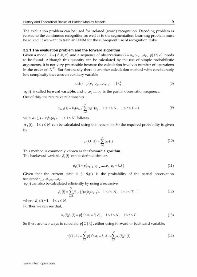
3.2.1 The evaluation problem and the forward algorithm

Given a model ( ), ,A Bλ π= and a sequence of observations 1 2, ,..., TO o o o= , { }|p O λ needs to be found. Although this quantity can be calculated by the use of simple probabilistic arguments, it is not very practicable because the calculation involves number of operations in the order of TN . But fortunately there is another calculation method with considerably low complexity that uses an auxiliary variable

{ }1 2( ) , ,..., , |t t ti p o o o q iα λ= = (8)

( )t iα is called forward variable, and 1 2, ,..., To o o is the partial observation sequence.

Out of this, the recursive relationship

1 1

1

( ) ( ) ( ) , 1 , 1 1N

t j t t iji

j b o i o j N t Tα α+ + == ≤ ≤ ≤ ≤ −∑ (9)

with 1 1( ) ( ), 1j jj b o j Nα π= ≤ ≤ follows.

( ), 1T i i Nα ≤ ≤ can be calculated using this recursion. So the required probability is given

by

{ }1

| ( )N

Ti

p O iλ α=

=∑ (10)

This method is commonly known as the forward algorithm. The backward variable ( )t iβ can be defined similar.

{ }1 2( ) , ,..., | ,t t t t ti p o o o q iβ λ+ += = (11)

Given that the current state is i, ( )t iβ is the probability of the partial observation sequence 1 2, ,...,t t To o o+ + .

( )t iβ can also be calculated efficiently by using a recursive

1 1

1

( ) ( ) ( ), 1 , 1 1N

t t ij j tj

i j a b o i N t Tβ β + +== ≤ ≤ ≤ ≤ −∑ (12)

where ( ) 1, 1T i i Nβ = ≤ ≤

Further we can see that,

{ }( ) ( ) , | , 1 , 1t t ti i p O q i i N t Tα β λ= = ≤ ≤ ≤ ≤ (13)

So there are two ways to calculate { }|p O λ , either using forward or backward variable:

{ } { }1 1

| , | ( ) ( )N N

t t ti i

p O p O q i i iλ λ α β= =

= = =∑ ∑ (14)

www.intechopen.com

Hidden Markov Models, Theory and Applications

10

This equation can be very useful, especially in deriving the formulas required for gradient based training.

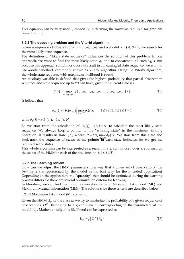
3.2.2 The decoding problem and the Viterbi algorithm

Given a sequence of observations 1 2, ,..., TO o o o= and a model ( ), ,A Bλ π= , we search for the most likely state sequence. The definition of “likely state sequence” influences the solution of this problem. In one approach, we want to find the most likely state tq and to concatenate all such ' tq 's. But because this approach sometimes does not result in a meaningful state sequence, we want to use another method, commonly known as Viterbi algorithm. Using the Viterbi algorithm, the whole state sequence with maximum likelihood is found. An auxiliary variable is defined that gives the highest probability that partial observation sequence and state sequence up to t=t can have, given the current state is i.

{ }1 2 1

1 2 1 1 2 1, ...

( ) max , ,..., , , , ,..., |t

t t t tq q q

i p q q q q i o o oδ λ−

− −= = (15)

It follows that

1 11

( ) ( ) max ( ) , 1 , 1 1t j t t iji N

j b o i a i N t Tδ δ+ + ≤ ≤⎡ ⎤= ≤ ≤ ≤ ≤ −⎢ ⎥⎣ ⎦ (16)

with 1 1( ) ( ), 1j jj b o j Nδ π= ≤ ≤

So we start from the calculation of ( ), 1T j j Nδ ≤ ≤ to calculate the most likely state sequence. We always keep a pointer to the ”winning state” in the maximum finding operation. It results in state *j , where

1* arg max ( )T

j Nj jδ≤ ≤= . We start from this state and

back-track the sequence of states as the pointer in each state indicates. So we get the required set of states. This whole algorithm can be interpreted as a search in a graph whose nodes are formed by the states of the HMM in each of the time instant , 1t t T≤ ≤ .

3.2.3 The Learning roblem

How can we adjust the HMM parameters in a way that a given set of observations (the training set) is represented by the model in the best way for the intended application? Depending on the application, the “quantity” that should be optimized during the learning process differs. So there are several optimization criteria for learning. In literature, we can find two main optimization criteria: Maximum Likelihood (ML) and Maximum Mutual Information (MMI). The solutions for these criteria are described below.

3.2.3.1 Maximum Likelihood (ML) criterion

Given the HMM wλ of the class w, we try to maximize the probability of a given sequence of observations wO , belonging to a given class w, corresponding to the parameters of the model wλ . Mathematically, this likelihood can be expressed as

{ }|wtot wL p O λ= (17)

www.intechopen.com

History and Theoretical Basics of Hidden Markov Models

11

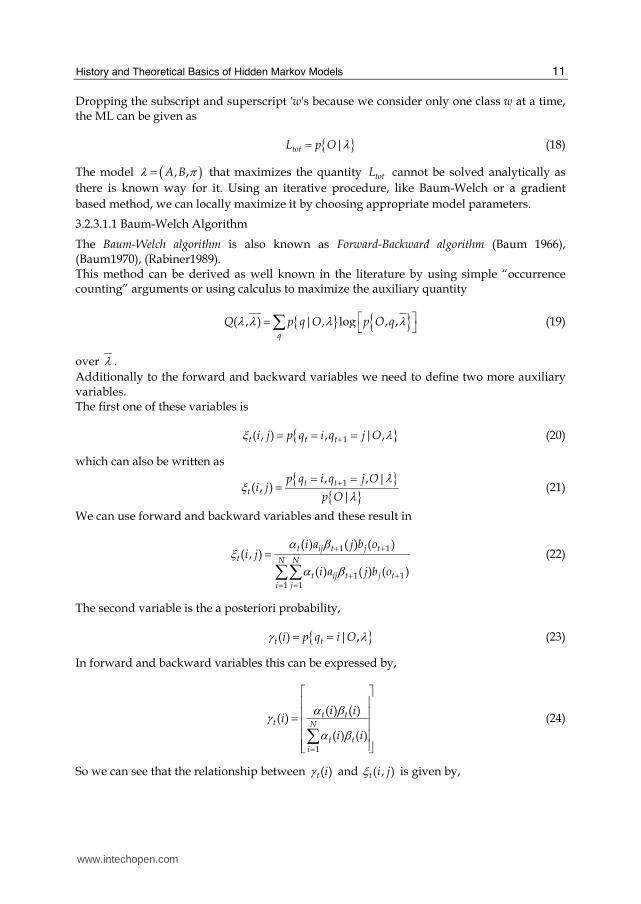
Dropping the subscript and superscript 'w's because we consider only one class w at a time, the ML can be given as

{ }|totL p O λ= (18)

The model ( ), ,A Bλ π= that maximizes the quantity totL cannot be solved analytically as there is known way for it. Using an iterative procedure, like Baum-Welch or a gradient based method, we can locally maximize it by choosing appropriate model parameters.

3.2.3.1.1 Baum-Welch Algorithm

The Baum-Welch algorithm is also known as Forward-Backward algorithm (Baum 1966), (Baum1970), (Rabiner1989). This method can be derived as well known in the literature by using simple “occurrence counting” arguments or using calculus to maximize the auxiliary quantity

{ } { }( , ) | , log , ,q

Q p q O p O qλ λ λ λ⎡ ⎤= ⎣ ⎦∑ (19)

over λ . Additionally to the forward and backward variables we need to define two more auxiliary variables. The first one of these variables is

{ }1( , ) , | ,t t ti j p q i q j Oξ λ+= = = (20)

which can also be written as

{ }{ }1, , |

( , )|

t tt

p q i q j Oi j

p O

λξ λ+= == (21)

We can use forward and backward variables and these result in

1 1

1 11 1

( ) ( ) ( )( , )

( ) ( ) ( )

t ij t j tt N N

t ij t j ti j

i a j b oi j

i a j b o

α βξα β

+ +

+ += =

=∑∑ (22)

The second variable is the a posteriori probability,

{ }( ) | ,t ti p q i Oγ λ= = (23)

In forward and backward variables this can be expressed by,

1

( ) ( )( )

( ) ( )

t tt N

t ti

i ii

i i

α βγα β

=

⎡ ⎤⎢ ⎥⎢ ⎥= ⎢ ⎥⎢ ⎥⎢ ⎥⎣ ⎦∑ (24)

So we can see that the relationship between ( )t iγ and ( , )t i jξ is given by,

www.intechopen.com

Hidden Markov Models, Theory and Applications

12

1

( ) ( , ), 1 , 1N

t tj

i i j i N t Mγ ξ=

= ≤ ≤ ≤ ≤∑ (25)

To maximize the quantity { }|p O λ , we can now describe the Baum-Welch learning process. We assume a starting model ( ), ,A Bλ π= and calculate the 'α 's and ' β 's. After this, we calculate the 'ξ 's and ' γ 's. The next equations are known as re-estimation formulas and are used to update the HMM parameters:

1( ), 1i i i Nπ γ= ≤ ≤ (26)

1

11

1

( , )

, 1 , 1

( )

T

tt

ij T

tt

i j

a i N j N

i

ξγ

−=−=

= ≤ ≤ ≤ ≤∑∑ (27)

1

1

( )

( ) , 1 , 1

( )

t k

T

tt

oj T

tt

j

b k j N k M

j

νγ

γ==

=

= ≤ ≤ ≤ ≤∑∑ (28)

These reestimation formulas can easily be modified to deal with the continuous density case too.

3.2.3.1.2 HMM Parameter Optimization

The optimization of the parameter κ of a given HMM λ is usually done by using Gradient related algorithms like shown in the following equation:

1

1

t

t t

κψκ κ ς κ −

− ∂⎡ ⎤= − ⎢ ⎥∂⎣ ⎦ (29)

By defining

{ }( )log p Oψ λ= − (30)

in order to find the maximum likelihood, the equation ψκ

∂∂ for any parameter κ of the HMM

λ has to be solved in order the minimized ψ .

The calculated ψ is therefore the expected Maximum Likelihood obtained by maximizing tκ .

By associating ψ to the HMM model parameters introduced above (see equation 14), we then obtain

{ }1 1

, ( ) ( )N N

tot t t ti i

L p O q i i iλ α β= =

= = =∑ ∑ (31)

www.intechopen.com

History and Theoretical Basics of Hidden Markov Models

13

The differentiation of the last equality in the equations (29) and (30) relative to the parameter κ of the HMM gives

1 tot

tot

L

L

ψκ κ

∂∂ = −∂ ∂ (32)

The Equation (32) calculates ψκ

∂∂ under the assumption, that totL

κ∂∂ is solvable. But this

derivative depends on all the actual parameter of the HMM. On the one side there are the transition probabilities , 1 ,ij i N jα ≤ ≥ and on the other side the observation probabilities { } { }( ), 1,..., , 1,...,jb k j N k M∈ ∈ . For this reason we have to find the derivative for the both probabilities sets and therefore their gradient.

a) Maximum likelihood gradient depending on transition probabilities

In order to calculate the gradient depending on transition probabilities, the Markov rule is usually assumed like following:

1

( )

( )

Tttot tot

ij t ijt

jL L

j

αα α α=

∂∂ ∂=∂ ∂ ∂∑ (33)

The simple differentiation

( )( )tot

tt

Lj

jβα

∂ =∂ (34)

as well as the time delay differentiation

1( )

( ) ( )tj t t

ij

jb i

α α αα −∂ =∂ (35)

gives after parameter substitutions the well known result

11

1( ) ( ) ( )

T

t j t tij tot t

j b iL

ψ β α αα −=∂ = −∂ ∑ (36)

b) Maximum Likelihood gradient depending on observation probabilities

In a similar matter as introduced above, the gradient depending on observation probabilities using the Markov rule is calculated. With

( )

( ) ( ) ( )ttot tot

j t t j t

jL L

b o j b o

αα

∂∂ ∂=∂ ∂ ∂ (37)

and

( ) ( )

( ) ( )t t

j t j t

j j

b o b o

α α∂ =∂ (38)

www.intechopen.com

Hidden Markov Models, Theory and Applications

14

the estimation probability is then calculated and results to

( ) ( )1

( ) ( )t t

j t tot j t

j j

b o L b o

α βψ∂ = −∂ . (39)

In the case of "Continuous Hidden-Markov-Models" or "Semi-Continuous Hidden-Markov-

Models" the densities , ,jm jm jm

c

ψ ψ ψμ

∂ ∂ ∂∂ ∂ ∂∑ are usually calculated similarly by just further

propagating the derivative ( )j tb o

ψ∂∂ assuming the Markov chain rules.

3.2.3.2 Maximum Mutual Information (MMI) criterion

Generally, in order to solve problems using Hidden Markov Models for example for engineering pattern recognition applications, there are two general types of stochastic optimization processes: on the one side, the Maximum Likelihood optimization process and on the other side the Maximum Mutual Information Process. The role of the Maximum Likelihood is to optimize the different parameters of a single given HMM class at a time independent of the HMM Parameters of the rest classes. This procedure will be repeated for every other HMM for each other class. In addition to the Maximum Likelihood, differences of the Maximum Mutual Infomation Methods are usually used in practice in order to solve the discrimination problematic in pattern recognition applications between every class that has to be recognized in a given problem. At the end one can obtain a special robust trained HMM-based system, thanks to the well known "discriminative training methodics". The basics of the Minimum Mutual Information calculations can be introduced by assuming a set of HMMs

{ }{ }, 1,...,Vνλ νΛ = ∈ (40)

of a given pattern recognition problem. The purpose of the optimization criterion will consist here of minimizing the "conditional uncertainty" ν of one "complete unit by a given real world problem" given an observation sequence sO of that class.

( ) { }, log ,s sI v O p v OΛ = − Λ (41)

This results in an art of minimization of the conditional entropy H, that can be also defined as the expectation of the conditional information I:

( ) { },sH V O E v O⎡ ⎤= Λ⎢ ⎥⎣ ⎦ (42)

in which V is the set of all classes and O is the set of all observation sequences. Therefore, the mutual information between the classes and observations

( ) ( ) ( )SH V O H V H V O= − (43)

www.intechopen.com

History and Theoretical Basics of Hidden Markov Models

15

is a maximized constant with ( )H V , hence the name "Maximum Mutual Information" criterion (MMI). In many literatures this technique is also well known as the "Maximum à Posteriori" method (MAP).

Generally Definition and Basics of the "Maximum à Posteriori" Estimation:

In Bayesian statistics, a maximum a posteriori probability (MAP) estimate is a mode of the posterior distribution. The MAP can be used to obtain a point estimate of an unobserved quantity on the basis of empirical data. It is closely related to Fisher's method of maximum likelihood (ML), but employs an augmented optimization objective which incorporates a prior distribution over the quantity one wants to estimate. MAP estimation can therefore be seen as a regularization of ML estimation.

Generally Description of the "Maximum à Posteriori" Estimation:

Assume that we want to estimate an unobserved Markov Model λ on the basis of observations o. By defining f as the sampling distribution of the observations o, so that ( )f o λ is the probability of o when the underlying Markov Model is λ . The function ( )f oλ λU can be defined as the likelihood function, so the estimate

ˆ ( ) arg max ( )ML o f oλ

λ λ= (44)

is the maximum likelihood estimate of the Markov Model λ . Now when we assume that a prior distribution χ over the models λ exists, we can treat λ as a random variable as in the classical Bayesian statistics. The posterior distribution of λ is therefore:

( )'

'

' ' '

( ) ( )

( ) ( )

f of o

f o

λ

λ χ λλ λ λ χ λ λ∈Λ

= ∂∫U (45)

where χ is the density function of λ and Λ is the domain of χ as application of the Bayes' theorem. The method of maximum a posteriori estimation then estimates the Markov Model λ as the mode of the posterior distribution of this random variable:

'

' ' '

( ) ( )ˆ ( ) arg max arg max ( ) ( )( ) ( )

ML

f oo f o

f oλ λλ

λ χ λλ λ χ λλ χ λ λ∈Λ

= =∂∫ (46)

The denominator of the posterior distribution does not depend on λ and therefore plays no role in the optimization. The MAP estimate of the Markov Modells λ coincides with the ML estimate when the prior χ is uniform (that is, a constant function). The MAP estimate is a limit of Bayes estimators under a sequence of 0-1 loss functions.

Application of the "Maximum à Posteriori" for the HMM

According to these basics of the "Maximum à Posteriori" above, the posteriori probability { },cp Oν Λ is maximised when the MMI criteria yields using the Bayes theorem to:

www.intechopen.com

Hidden Markov Models, Theory and Applications

16

{ } { }{ } { }{ }ΛΛ−=ΛΛ−=Λ−==

c

c

c

c

s

MMIMAPOp

Op

Op

OpOvpEE

,

,log

,log,log ω

νν

(47)

where ω is any possible class. By using similar notation as in (17), the likelihoods can be written as following:

{ },correct ctotL p Oν λ= (48)

{ },others ctotL p O

ωω λ=∑ (49)

where indices "correct" and "others" distinguish between the correct class and all the other classes. From the both equation above we then obtain expectations of the MMI or MAP as:

logcorrecttot

MAP MMI othertot

LE E

L= = − (50)

In analogy to the Maximum Likelihood, in order to minimize MMIE , we can assume that

MMIEψ = , and derive the gradients after ψκ

∂∂ using the well known gradient related

algorithms, where κ is an arbitrary parameter of the whole set of HMMs, Λ . In analogy to the Maximum Likelihood estimation methods above, we then obtain

κκκ

ψ∂

∂−∂∂=∂

∂ correct

tot

correct

tot

others

tot

others

tot

L

L

L

L

11

(51)

with ( ) ( )correcttot t t

i class

L i iυα β

∈= ∑ and ( ) ( )others

tot t ti class w

L i iω

α β∈

=∑ ∑ .

With the same procedure as for the Maximum Likelihood, the transition and observation probabilities must also be calculated as illustrated in the next steps by using the general law of the Markov chain.

a) Maximum Mutual Information gradient depending on transition probabilities

By using the well known Kronecker symbol kvδ , the calculation basics then yields to

( ) ( )

1

( )

( )

correct or others correct or othersTttot tot

ij t iji

jL L

j

αα α α=

∂∂ ∂=∂ ∂ ∂∑ (52)

with

( )

11

( ) ( ) ( )correct Ttot

kv t j t tij i

Lj b o i

i class k

δ β αα −=∂ = ∂∂∈

∑ (53)

www.intechopen.com

History and Theoretical Basics of Hidden Markov Models

17

and

( )

11

( ) ( ) ( )others T

tott j t t

ij i

Lj b o iβ αα −=

∂ =∂ ∑ (54)

After simplification one obtain

1( ) ( )1

1( ) ( ) ( )

Tkv

t j t tothers correctij itot tot

j b o iL L

i class k

δψ β αα −=⎡ ⎤∂ = −⎢ ⎥∂ ⎢ ⎥⎣ ⎦

∈∑ . (55)

b) Maximum Mutual Information gradient depending on observation probabilities

The calculation of the Maximum Mutual Information gradient depending on observation probabilities is similar to the description above according to the Markov chain rules as following:

( ) ( ) ( )

( ) ( ) ( )

correct or others correct or othersttot tot

j t t j t

jL L

b o j b o

αα

∂∂ ∂=∂ ∂ ∂ . (56)

After differentiation after ( )t jα and simplification using the Kronecker function kvδ , the "correct" as well as the "others" variant are extracted usually as following:

( ) ( )

( ) ( )

correctt ttot

kvj t j t

j jL

b o b o

j class k

α βδ∂ =∂∈

(57)

and

( ) ( )

( ) ( )

otherst ttot

j t j t

j jL

b o b o

α β∂ =∂ (58)

After further simplifications one obtain

( ) ( )1

( ) ( )t tkv

others correctj t j ttot tot

j j

b o b oL L

j class k

α βδ⎡ ⎤∂Ψ = −⎢ ⎥∂ ⎢ ⎥⎣ ⎦∈

(59)

With ( ) ( )

( )correct t tt kv correct

tot

j jj

L

j class k

α βγ δ=∈

and ( ) ( )

( )others t tt correct

tot

j jj

L

α βγ =

follows:

1

( ) ( )( ) ( )

others correctt t

j t j t

j jb o b o

γ γ∂Ψ ⎡ ⎤= −⎣ ⎦∂ . (60)

www.intechopen.com

Hidden Markov Models, Theory and Applications

18

4. Types of Hidden Markov Models

Nowadays, depending on problem complexities, signal processing requirements and applications, it is indispensable to choose the appropriate type of HMM very early in the concept and design phase of modern HMM based systems. In this part different types of HMMs will be introduced and some generalized criteria will be shown for how to choose the right type in order to solve different kinds of problems (Huang1989), (Kouemou2008), (Rabiner1989).

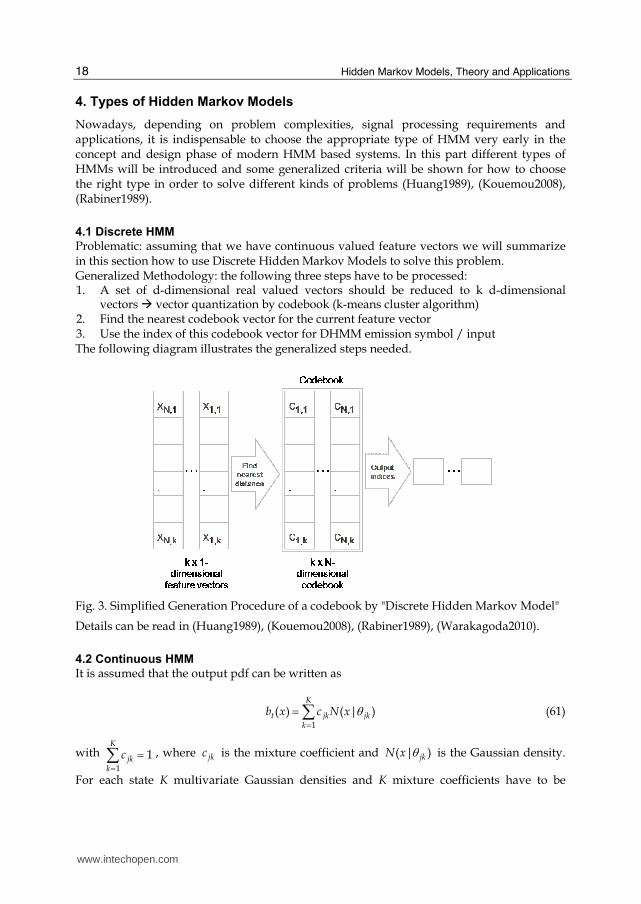
4.1 Discrete HMM

Problematic: assuming that we have continuous valued feature vectors we will summarize in this section how to use Discrete Hidden Markov Models to solve this problem. Generalized Methodology: the following three steps have to be processed: 1. A set of d-dimensional real valued vectors should be reduced to k d-dimensional

vectors å vector quantization by codebook (k-means cluster algorithm) 2. Find the nearest codebook vector for the current feature vector 3. Use the index of this codebook vector for DHMM emission symbol / input The following diagram illustrates the generalized steps needed.

Fig. 3. Simplified Generation Procedure of a codebook by "Discrete Hidden Markov Model"

Details can be read in (Huang1989), (Kouemou2008), (Rabiner1989), (Warakagoda2010).

4.2 Continuous HMM

It is assumed that the output pdf can be written as

1

( ) ( | )K

t jk jkk

b x c N x θ=

=∑ (61)

with 1

1K

jkk

c=

=∑ , where jkc is the mixture coefficient and ( | )jkN x θ is the Gaussian density.

For each state K multivariate Gaussian densities and K mixture coefficients have to be

www.intechopen.com

History and Theoretical Basics of Hidden Markov Models

19

estimated. This result in the following parameters for each state: covariance matrix, mean vector and mixture coefficients vector. A continuous Hidden Markov Model is a three-layered stochastic process. The first part is, equal to DHMM, the selection of the next state. The second and the third part are similar to the selection of emission symbol with DHMM, whereas the second part of CHMM is the selection of the mixture density by mixture coefficient. The selection of the output symbol (vector) by the Gaussian density is the third and last part. The classification and training algorithms have to be modified. There are only minor changes in the classification algorithm: the modified probability densities have to be substituted. The Baum-Welch/Viterbi trainings algorithms have to be modified by additional calculation. The disadvantage is a high computational effort. The Gaussian distributions have to be evaluated and the high number of parameters probably may result in instabilities.

Fig. 4. Illustration of exemplary statistical distributions by continuous "Hidden Markov Models"

Details can be read in (Huang1989), (Kouemou2008), (Rabiner1989), (Warakagoda2010).

4.3 Semi-continuous HMM

The semi-continuous HMM can be seen as a compromise between DHMM and CHMM. It is assumed that the output pdf can be written as

1

( ) ( | )K

t jk kk

b x c P x θ=

=∑ (62)

with 1

1K

jkk

c=

=∑ , where jkc is the mixture coefficient and ( | )kP x θ the Gaussian distribution.

Overall, K multivariate Gaussian distributions and K mixture coefficients have to be estimated. In contrast to the CHMM, we the same set of Gaussian mixture densities is used for all states.

www.intechopen.com

Hidden Markov Models, Theory and Applications

20

Fig. 5. Simple Illustration of the densities distribution CHMM vs. SCHMM.

Like the CHMM, the SCHMM is a three-layered stochastic process. After the next state has been selected, there will be the selection of the mixture density by the mixture coefficient. Third, the output symbol (vector) has to be selected by Gaussian density. The second and third step is similar to the selection of emission symbol with DHMM. There have to be some modifications of classification and training algorithms, too. For classification algorithm, the modified probability densities have to be modified and the Baum-Welch/Viterbi training algorithm are modified by additional calculations. The disadvantage is a high computational effort. The Gaussian distributions have to be evaluated and the high number of parameters probably may result in instabilities. Altogether, the modifications are similar to those in the CHMM, but the number of parameters is reduces significantly. Details can be read in (Huang1989), (Kouemou2008), (Rabiner1989), (Warakagoda2010).

5. Basics of HMM in modern engineering processing applications

Nowadays, Hidden Markov Models are used in a lot of well-known systems all over the world. In this part of the chapter some general recommendations to be respected by creating an HMM for operational applications will first be introduced, followed by practical examples in the financial word, bioinformatics and speech recognition. This chapter part consists of the following under chapters: • 5.1. General recommendations for creating HMMs in the practice • 5.2. Application Examples in Financial Mathematics World, Bank and Assurances • 5.3. Application Example in Bioinformatics and Genetics • 5.4. Speech recognition and further Application Examples

5.1 General recommendations for creating HMMs in the practice 5.1.1 Creation of HMM architecture

The basis for creating an HMM for practical applications is a good understanding of the real world problem, e.g. the physical, chemical, biological or social behaviour of the process that should be modelled as well as its stochastic components. The first step is to check if the laws for Markov chains are fulfilled, that means if it is a Markov process as defined above. If these laws are fulfilled, exemplary models can be structured with the help of the understanding of the relationships between the states of each Markov Model. Deterministic and stochastic characteristics in the process shall be clearly separated. After all of these steps are executed, the technical requirements of the system also have to be taken into consideration. It is very important to consider the specification of the signal processor in the running device.

www.intechopen.com

History and Theoretical Basics of Hidden Markov Models

21

5.1.2 Learning or adapting an HMM to a given real problem

First of all, different elements of the real problem to be analyzed have to be disaggregated in a form of Markov models. A set of Hidden Markov Models has to be defined that represents the whole real world problem. There are several points that have to be kept in mind, e.g. What should be recognized?, What is the input into the model, what is the output? The whole learning process is done in two steps. In the first step learning data have to be organized, e.g. by performing measurements and data recording. If measurement is too complex or not possible, one can also recommend using simulated data. During the second step the learning session is started, that means the Markov parameters as explained in the chapters above are adapted.

5.2 Application examples in financial mathematics world, bank and assurances

Nowadays, many authors are known from literature for using HMMs and derivative in order to solve problems in the world of financial mathematics, banking and assurance (Ince2005), (Knab2000), (Knab2003), (Wichern2001). The following example was published by B. Knapp et.al. “Model-based clustering with Hidden Markov Model and its application to financial time-series data” and presents a method for clustering data which must be performed well for the task of generating statistic models for prediction of loan bank customer collectives. The generated clusters represent groups of customers with similar behaviour. The prediction quality exceeds the previously used k-mean based approach. The following diagram gives an overview over the results of their experiment:

Fig. 6. Example of a Hidden Markov Model used by Knap et.al. in order to model the three phases of a loan banking contract

5.3 Application example in bioinformatics and genetics

Other areas where the use of HMMs and derivatives becomes more and more interesting are biosciences, bioinformatics and genetics (Asai1993), (Schliep2003), (Won2004), (Yada1994), (Yada1996), (Yada1998). A. Schliep et al., presented 2003 for example, in the paper “Using hidden Markov models to analyze gene expression time course data”, a practical method which aim "to account for the

www.intechopen.com

Hidden Markov Models, Theory and Applications

22

Fig. 7. Exemplary results of Knap et.al: examined “sum of relative saving amount per sequence” of the real data of bank customers and a prediction of three different models.

Fig. 8. Flow diagram of the Genetic Algorithm Hidden Markov Models (GA-HMM) algorithm according to K.J. Won et.al.

horizontal dependencies along the time axis in time course data" and "to cope with the prevalent errors and missing values" while observing, analysing and predicting the behaviour of gene data. The experiments and evaluations were simulated using the "ghmm-software", a freely available tool of the "Max Planck Institute for Molecular Genetics", in Berlin Germany (GHMM2010). K.J. Won et.al. presented, 2004, in the paper “Training HMM Structure with Genetic Algorithm for Biological Sequence Analysis” a training strategy using genetic algorithms for HMMs (GA-HMM). The purpose of that algorithm consists of using genetic algorithm and is tested on finding HMM structures for the promoter and coding region of the bacterium

www.intechopen.com

History and Theoretical Basics of Hidden Markov Models

23

C.jejuni. It also allows HMMs with different numbers of states to evolve. In order to prevent over-fitting, a separate data set is used for comparing the performance of the HMMs to that used for the Baum-Welch-Training. K.J. Won et.al. found out that the GA-HMM was capable of finding an HMM, comparable to a hand-coded HMM designed for the same task. The following figure shows the flow diagram of the published GA-HMM algorithm.

Fig. 9. Result during GA-HMM training after K.J. Won et.al.: (a) shows the fitness value of fittest individual on each iteration (b) shows average number of states for periodic signal. The GA started with a population consisting of 2 states. After 150 generations the HMM have a length of 10 states. Although the length does not significantly change thereafter the fitness continues to improve indicating that the finer structure is being fine tuned.

Fig. 10. Exemplary result of the GA-HMM structure model for a given periodic signal after training the C.jejuni sequences (K.J. Won).

5.4 Speech recognition and further application examples

Hidden Markov Models are also used in many other areas in modern sciences or engineering applications, e.g. in temporal pattern recognition such as speech, handwriting, gesture recognition, part-of-speech tagging, musical score following, partial discharges. Some authors even used HMM in order to explain or predict the behaviour of persons or group of persons in the area of social sciences or politics (Schrodt1998). One of the leading application area were the HMMs are still predominant is the area of "speech recognition" (Baum1970), (Burke1958), (Charniak1993), (Huang1989), (Huang1990), (Lee1989,1), (Lee1989,2), (Lee1990), (Rabiner1989). In all applications presented in this chapter, the "confusions matrices" is widely spread in order to evaluate the performance of HMM-based-Systems. Each row of the matrix represents the instances in a predicted class, while each column represents the instances in an actual class. One benefit of a confusion matrix is that it is easy to see if the system is confusing two classes (i.e. commonly mislabelling one as another). When a data set is

www.intechopen.com

Hidden Markov Models, Theory and Applications

24

unbalanced, this usually happens when the number of samples in different classes varies greatly, the error rate of a classifier is not representative of the true performance of the classifier. This can easily be understood by an example: If there are 980 samples from class 1 and only 20 samples from class 2, the classifier can easily be biased towards class 1. If the classifier classifies all the samples as class 1, the accuracy will be 98%. This is not a good indication of the classifier's true performance. The classifier has a 100% recognition rate for class 1 but a 0% recognition rate for class 2. The following diagram shows a simplified confusion-matrix of a specified character recognition device for the words "A","B","C","D","E" of the German language using a very simple "HMM-Model", trained data from 10 different persons and tested on 20 different persons, only for illustration purpose.

"A" 99,5 0 0 0 0 0,5

"B" 0 95 1,4 1,6 0,5 1,5

"C" 0 1,7 95,1 1,3 0,7 1,2

"D" 0 1 1,6 95,7 0,4 1,3

"Pred

icted" or "labeled

as" "E" 0 0,1 0,05 0,05 99,6 0,2

"A" "B" "C" "D" "E" rejected

"Actual" or "Recognized as" or "Classified as"

Table: Example of a Confusion Matrix for simple word recognition in the German language.

Depending on the values of the confusion matrix one call also derive typical performances of the HMM-based automate like: the general correct classification rate, the general false classification rate, the general confidences or sensitivities of the classifiers.

6. Conclusion

In this chapter the history and fundamentals of Hidden Markov Models were shown. The important basics and frameworks of mathematical modelling were introduced. Furthermore, some examples of HMMs and how they can be applied were introduced and discussed focussed on real engineering problems. For more detailed analysis a considerable list of literature and state of the art is given.

7. References

Asai, K. & Hayamizu, S. & Handa, K. (1993). Prediction of protein secondary structure by the hidden Markov model. Oxford Journals Bioinformatics, Vol. 9, No. 2, 142-146

Baum, L.E. & Petrie, T. (1966). Statistical inference for probabilistic functions of finite Markov chains. The Annals of Mathematical Statistics, Vol. 37, No. 6, 1554-1563.

www.intechopen.com

History and Theoretical Basics of Hidden Markov Models

25

Baum, L.E. et al. (1970). A maximization technique occurring in the statistical analysis of probabilistic functions of Markov chains, The Annals of Mathematical Statistics, Vol. 41, No. 1, 164–171.

Bayes, T. & Price, R. (1763). An Essay towards solving a Problem in the Doctrine of Chances, In: Philosophical Transactions of the Royal Society of London 53, 370-418.

Burke, C. J. & Rosenblatt,M(1958). A Markovian Function of a Markov Chain. The Annals of Mathematical Statistics, Vol. 29, No. 4, 1112-1122.

Charniak, E.(1993). Statistical Language Learning, MIT Press, ISBN-10: 0-262-53141-0, Cambridge, Massachusetts.

Foellinger, O. (1992). Regelungstechnik, 7. Auflage, Hüthig Buch Verlag Heidelberg.GHMM, (2010). LGPL-ed C library implementing efficient data structures and algorithms for basic and extended HMMs. Internet connection: URL: http://www.ghmm.org. [14/08/2010]

Huang, X.D & Jack, M.A. (1989). Semi-continuous hidden Markov models for speech recognition, Ph.D. thesis, Department of Electrical Engineering, University of Edinburgh.

Huang,X. D. &Y. Ariki & M. A. Jack (1990). Hidden Markov Models for Speech Recognition. Edinburgh University Press.

Ince, H. T. & Weber, G.W. (2005). Analysis of Bauspar System and Model Based Clustering with Hidden Markov Models, Term Project in MSc Program “Financial Mathematics – Life Insurance”, Institute of Applied Mathematics METU

Kalman, R.(1960): A New Approach to Linear Filtering and Prediction Problems. In: Transactions of the ASME-Journal of Basic Engineering

Kolmogorov, A. N. (1931). Über die analytischen Methoden in der Wahrscheinlichkeits-rechnung, In: Mathematische Annalen 104, 415.

Knab, B. (2000) Erweiterungen von Hidden-Markov-Modellen zur Analyse oekonomischer Zeitreihen. Dissertation, University of Cologne

Knab, B. & Schliep, A. & Steckemetz, B. & Wichern, B. (2003). Model-based clustering with Hidden Markov Models and its application to financial time-series data.

Kouemou, G. (2000). Atemgeräuscherkennung mit Markov-Modellen und Neuronalen Netzen beim Patientenmonitoring, Dissertation, University Karlsruhe.

Kouemou, G. et al. (2008). Radar Target Classification in Littoral Environment with HMMs Combined with a Track Based classifier, Radar Conference, Adelaide Australia.

Kouemou, G. (2010). Radar Technology, G. Kouemou (Ed.), INTECH, ISBN:978-953-307 029-2. Lee, K.-F. (1989) "Large-vocabulary speaker-independent continuous speech recognition:

The SPHINX system", Ph.D. thesis, Department of Computer Science, Carnegie-Mellon University.

Lee, K.-F. (1989) Automatic Speech Recognition. The Development of the SPHINX System, Kluwer Publishers, ISBN-10: 0898382963, Boston, MA.

Lee, K.-F.(1990) Context-dependent phonetic hidden Markov models for speakerindependent continuous speech recognition, Morgan Kaufmann Publishers, Inc., San Mateo, CA, 1990.

Markov, A. A. (1908). Wahrscheinlichkeitsrechnung, B. G. Teubner, Leipzig, Berlin Petrie, T (1966). Probabilistic functions of finite state Markov chains. The Annals of

Mathematical Statistics, Vol. 40, No. 1,:97-115.

www.intechopen.com

Hidden Markov Models, Theory and Applications

26

Rabiner,L.R. & Wilpon, J.G. & Juang, B.H, (1986). A segmental k-means training procedure for connected word recognition, AT&T Technical Journal, Vol. 65, No. 3, pp.21-40

Rabiner, L. R. (1989). A tutorial on hidden Markov models and selected applications in speech recognition. Proceedings of the IEEE, Vol. 77, No. 2, 257-286.

Schliep, A.& Schönhuth, A. & Steinhoff, C. (2003). Using Hidden Markov Models to analyze gene expression time course data, Bioinformatics, Vol. 19, No. 1: i255–i263.

Schrodt, P. A. (1998). Pattern Recognition of International Crises using Hidden Markov Models, in D. Richards (ed.), Non-linear Models and Methods in Political Science, University of Michigan Press, Ann Arbor, MI.

Viterbi, A. (1967). Error bounds for convolutional codes and an asymptotically optimum decoding algorithm, In: IEEE Transactions on Information Theory. 13, Nr. 2,pp.260-269

Warakagoda, Narada (2009). Hidden Markov Models, internet connection, URL: http://jedlik.phy.bme.hu/~gerjanos/HMM/node2.html [14/08/2010]

Wichern, B (November 2001). Hidden-Markov-Modelle zur Analyse und Simulation von Finanzzeitreihen. PhD thesis. Cologne University

Wikipedia1, (2010). http://en.wikipedia.org/wiki/Andrey_Markov [20/08/2010] Wikipedia2, (2010). http://en.wikipedia.org/wiki/Hidden_Markov_model [14/08/2010] Wikipedia3, (2010). http://en.wikipedia.org/wiki/Markov_chain [14/08/2010] Wikipedia4, (2010). http://en.wikipedia.org/wiki/Markov_process [14/08/2010] Won, K..J. & Prügel-Bennett, A. & Krogh, A. (2004). Training HMM Structure with Genetic

Algorithm for Biological Sequence Analysis, Bioinformatics, Vol. 20, No. 18, 3613-3619

Yada,T. & Ishikawa,M. & Tanaka,H. & Asai, K(1994). DNA Sequence Analysis using Hidden Markov Model and Genetic Algorithm. Genome Informatics, Vol.5, pp.178-179.

Yada, T. & Hirosawa, M. (1996). Gene recognition in cyanobacterium genomic sequence data using the hidden Markov model, Proceedings of the Fourth International Conference on Intelligent Systems for Molecular Biology, AAAI Press, Menlo Park, pp. 252–260.

Yada, T. (1998) Stochastic Models Representing DNA Sequence Data - Construction Algorithms and Their Applications to Prediction of Gene Structure and Function. Ph.D. thesis, University of Tokyo.

The author would like to thank his family {Dr. Ariane Hack (Germany), Jonathan Kouemou (Germany), Benedikt Kouemou (Germany)} for Supporting and Feedbacks.

Ulm, Germany, September 2010.

www.intechopen.com

Hidden Markov Models, Theory and ApplicationsEdited by Dr. Przemyslaw Dymarski

ISBN 978-953-307-208-1Hard cover, 314 pagesPublisher InTechPublished online 19, April, 2011Published in print edition April, 2011

InTech EuropeUniversity Campus STeP Ri Slavka Krautzeka 83/A 51000 Rijeka, Croatia Phone: +385 (51) 770 447 Fax: +385 (51) 686 166www.intechopen.com

InTech ChinaUnit 405, Office Block, Hotel Equatorial Shanghai No.65, Yan An Road (West), Shanghai, 200040, China

Phone: +86-21-62489820 Fax: +86-21-62489821

Hidden Markov Models (HMMs), although known for decades, have made a big career nowadays and are stillin state of development. This book presents theoretical issues and a variety of HMMs applications in speechrecognition and synthesis, medicine, neurosciences, computational biology, bioinformatics, seismology,environment protection and engineering. I hope that the reader will find this book useful and helpful for theirown research.

How to referenceIn order to correctly reference this scholarly work, feel free to copy and paste the following:

Guy Leonard Kouemou (2011). History and Theoretical Basics of Hidden Markov Models, Hidden MarkovModels, Theory and Applications, Dr. Przemyslaw Dymarski (Ed.), ISBN: 978-953-307-208-1, InTech,Available from: http://www.intechopen.com/books/hidden-markov-models-theory-and-applications/history-and-theoretical-basics-of-hidden-markov-models

© 2011 The Author(s). Licensee IntechOpen. This chapter is distributedunder the terms of the Creative Commons Attribution-NonCommercial-ShareAlike-3.0 License, which permits use, distribution and reproduction fornon-commercial purposes, provided the original is properly cited andderivative works building on this content are distributed under the samelicense.