HMA PAY ADJUSTMENT - New Jersey · HMA PAY ADJUSTMENT FINAL REPORT June 2015 ... Dr. Nick Vitillo...

FHWA-NJ-2015-007

HMA PAY ADJUSTMENT

FINAL REPORT June 2015

Submitted by

Hao Wang, Ph.D. Assistant Professor Rutgers University

Zilong Wang Graduate Research Assistant

Rutgers University

Thomas Bennert, Ph.D. Associate Research Professor

Rutgers University

Richard Weed Consultant

Advanced Infrastructure Design, Inc.

NJDOT Research Project Manager Smmamunar Rashid

In cooperation with

New Jersey Department of Transportation

Bureau of Research And

U. S. Department of Transportation Federal Highway Administration

DISCLAIMER STATEMENT The contents of this report reflect the views of the authors who are responsible for the facts and the accuracy of the data presented herein. The contents do not necessarily reflect the official views or policies of the New Jersey Department of Transportation or the Federal Highway Administration. This report does not constitute a standard, specification, or regulation.

i

TECHNICAL REPORT STANDARD TITLE PAGE

1. Report No. 2.Government Accession No. 3. Recipient’s Catalog No. FHWA NJ-2015-007

4. Title and Subtitle 5. Report Date HMA PAY ADJUSTMENT

June 2015

6. Performing Organization Code

7. Author(s) 8. Performing Organization Report No.

Hao Wang Ph.D., Zilong Wang, Thomas Bennert Ph.D., and Richard Weed

9. Performing Organization Name and Address 10. Work Unit No. Center for Advanced Infrastructure and Transportation Rutgers, The State University of New Jersey 100 Brett Road Piscataway, NJ 08854

11. Contract or Grant No.

12. Sponsoring Agency Name and Address 13. Type of Report and Period Covered

Final Report July 2012 – December 2014 14. Sponsoring Agency Code

15. Supplementary Notes 16. Abstract The objective is to evaluate multiple quality characteristics of hot-mix asphalt (HMA) and develop performance-related pay adjustment. An extensive literature review was conducted to review the current state-of-practice on quality acceptance and performance-related specifications. Construction data and pavement performance data were collected for a large number of projects in New Jersey. The performance-related pay adjustment for in-place air void was developed using life-cycle cost analysis (LCCA). Laboratory tests were conducted to measure air voids and permeability of field cores taken at the longitudinal joint to determine the upper limits of air voids at the longitudinal joint. Alternative pay equations for air voids at the longitudinal joint were evaluated using risk analysis. Pavement structural analysis was conducted to predict the interface shear stress under vehicular loading to identify the minimum bonding strength requirement to prevent premature pavement failure. Future research is recommended to refine the longitudinal joint density specification and quantify the relationship between interface bonding and the expected pavement life. 17. Key Words 18. Distribution Statement Quality Assurance, Pay Adjustment, In-Place Air Void, Longitudinal Joint, Interface Bonding, Life-Cycle Cost Analysis, Pavement Performance

No Restrictions

19. Security Classif (of this report) 20. Security Classif. (of this page)

21. No of Pages 22. Price

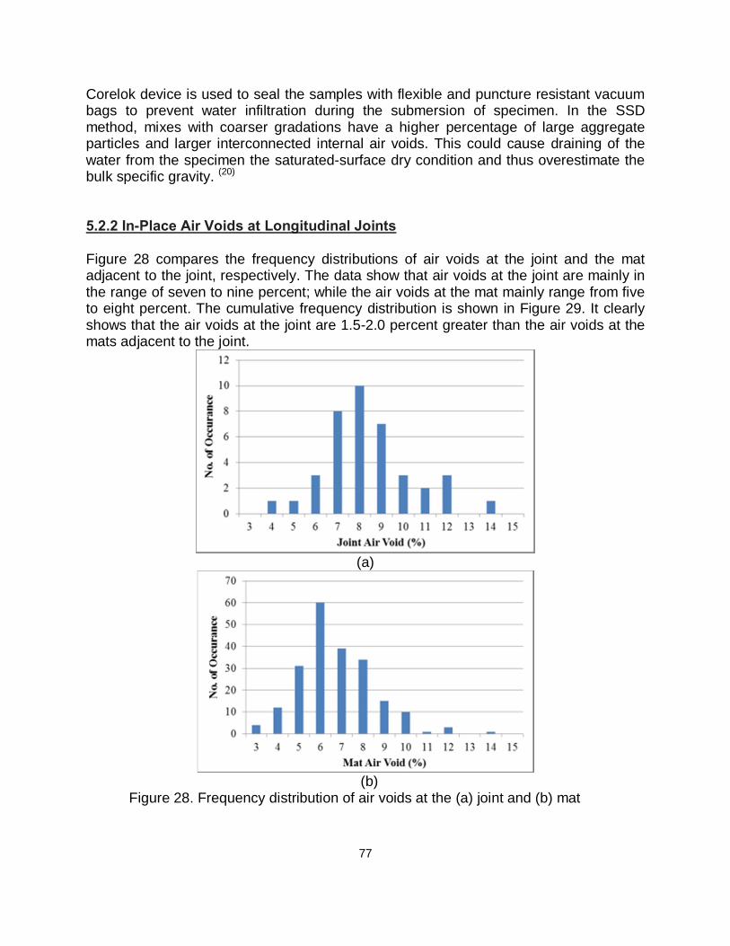
Unclassified Unclassified 128 Form DOT F 1700.7 (8-69)

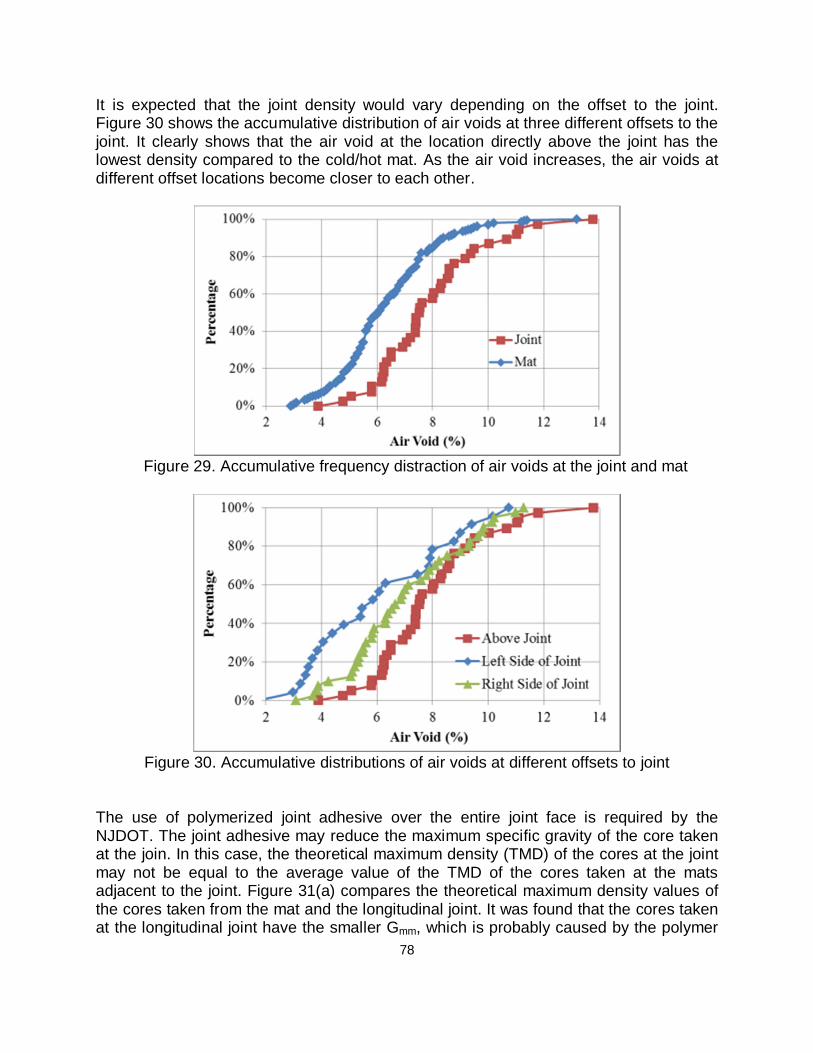
Federal Highway Administration U.S. Department of Transportation Washington, D.C.

New Jersey Department of Transportation 1035 Parkway Avenue P.O. Box 600 Trenton, NJ 08625

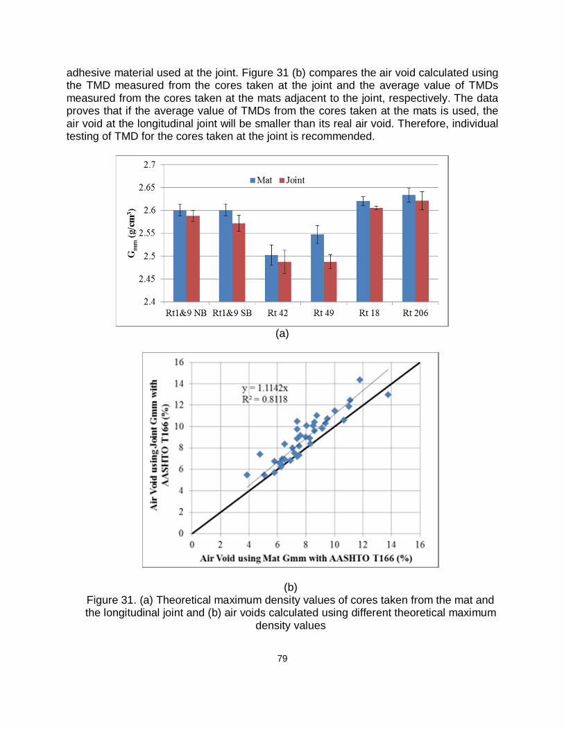
ii

ACKNOWLEDGEMENT This project was sponsored by the New Jersey Department of Transportation (NJDOT) and the Federal Highway Administration. This project could not have been accomplished without the assistance of numerous individuals. The authors would like to express gratitude to Smmamunar Rashid, Daniel LiSanti, Robert J. Blight, Susan Gresavage, and Eileen C. Sheehy with NJDOT, Dr. Nick Vitillo with Rutgers University, and Vivek Jha, Robert Sauber, and Dr. Kaz Tabrizi with Advanced Infrastructure Design, Inc.

.

iii

TABLE OF CONTENTS 1. EXECUTIVE SUMMARY ............................................................................................ 1 2. INTRODUCTION ......................................................................................................... 5

2.1 Background ....................................................................................................... 5 2.2 Objective............................................................................................................ 6

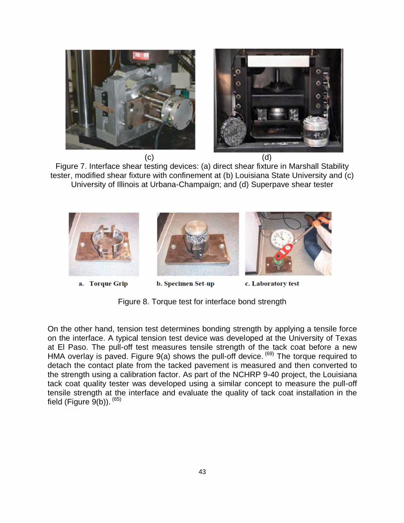
3. LITERATURE REVIEW .............................................................................................. 7 3.1 Review of Specifications for Pavement Construction ................................... 7 3.2 Acceptance Procedure and Pay Factors ...................................................... 11 3.3 HMA Quality Characteristics and Test Methods .......................................... 19 3.4 Performance-Related Pay Adjustment .......................................................... 24 3.5 Longitudinal Joint Density Specification ..................................................... 34 3.6 Interface Bond Strength ................................................................................. 42

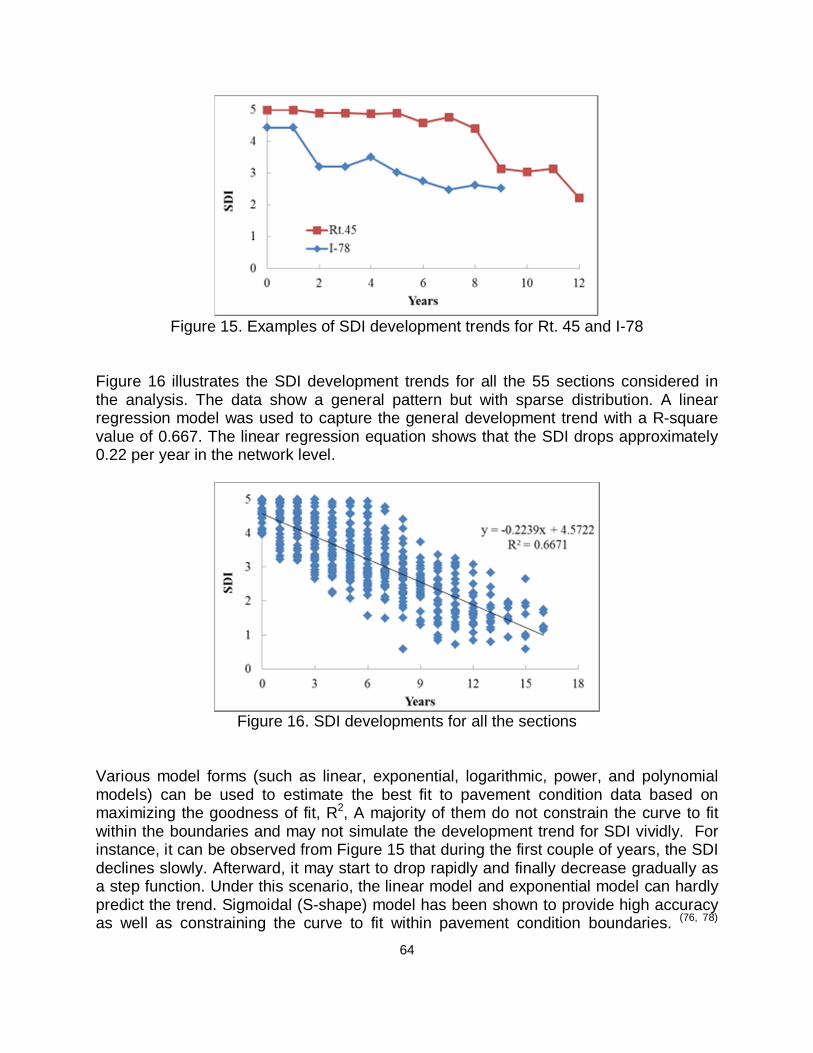
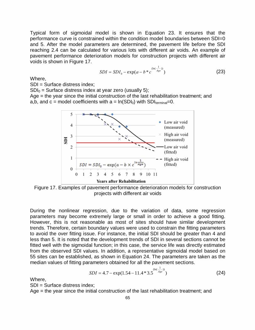
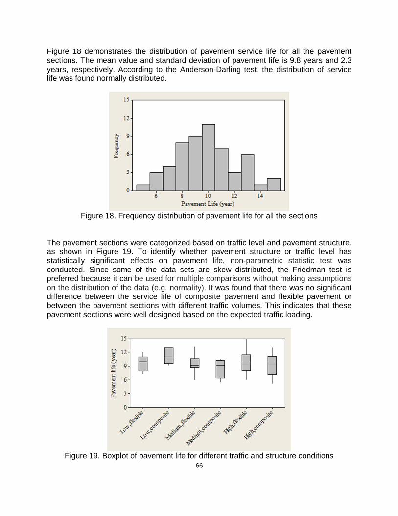
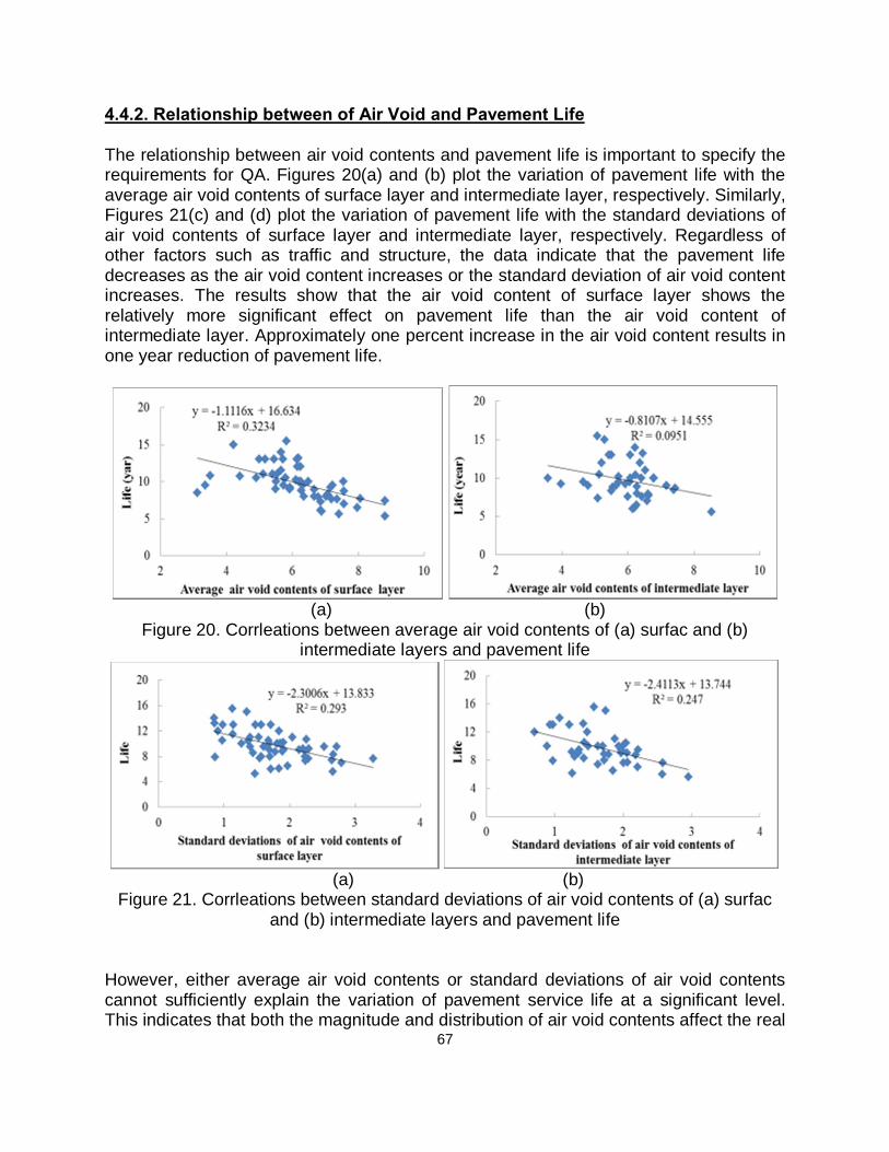
4. PAY ADJUSTMENT FOR IN-PLACE AIR VOID ...................................................... 57 4.1 Methodology ................................................................................................... 57 4.2 Analysis of Air Void Data ............................................................................... 58 4.3 Pay Adjustment using Current NJDOT Specification .................................. 60 4.4 Development of LCCA-Based Pay Adjustment ............................................ 63

5. PAY ADJUSTMENT FOR LONGITUDINAL JOINT DENSITY ................................. 73 5.1 Construction of Longitudinal Joints ............................................................. 73 5.2 Joint Density Testing and Results ................................................................ 74 5.3 Statistical Analyses using SPECRISK .......................................................... 83

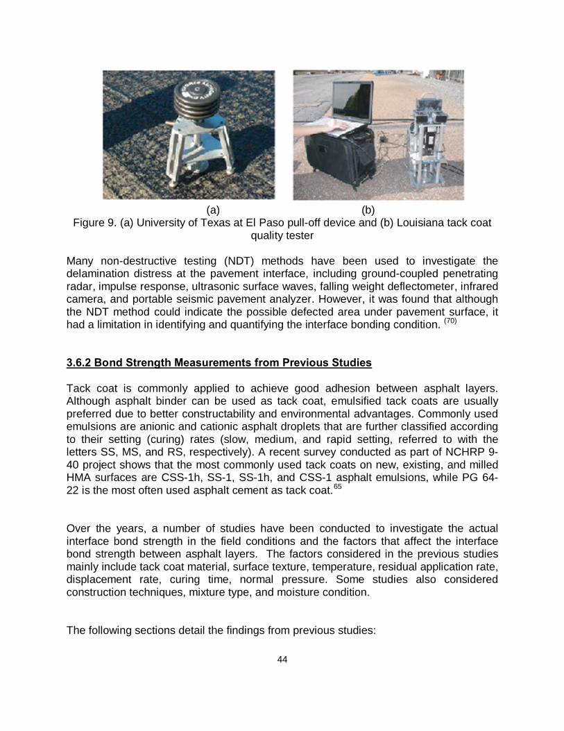
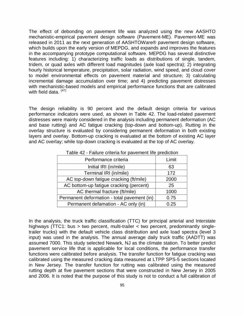
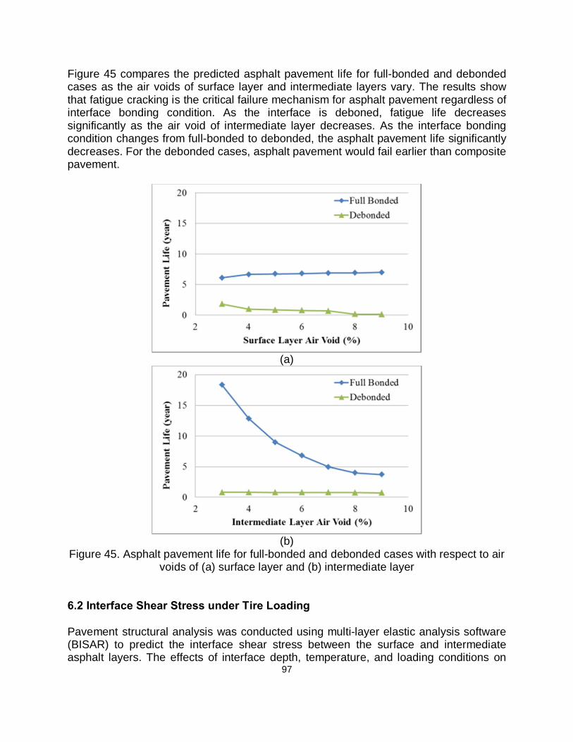
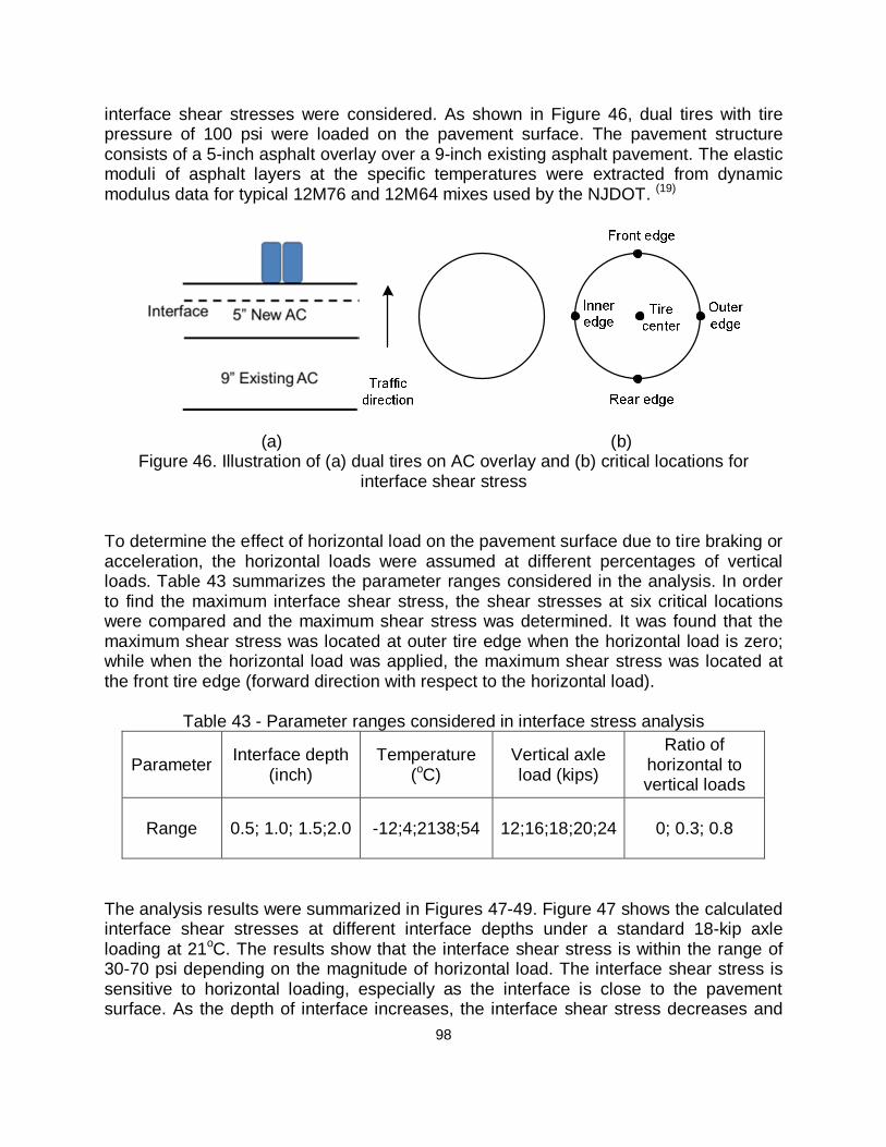
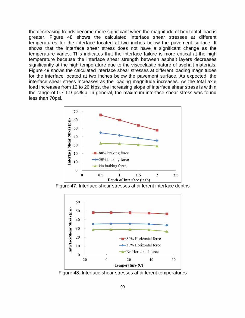
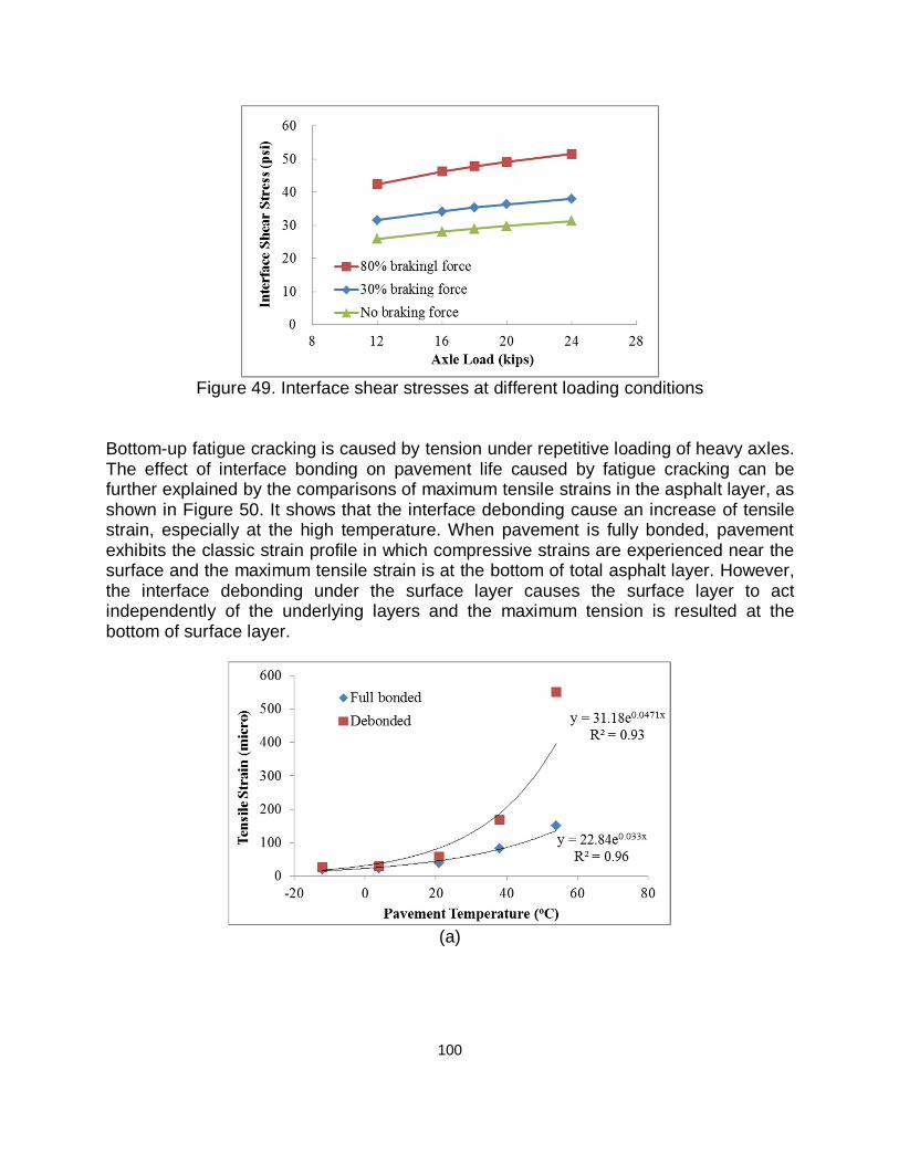
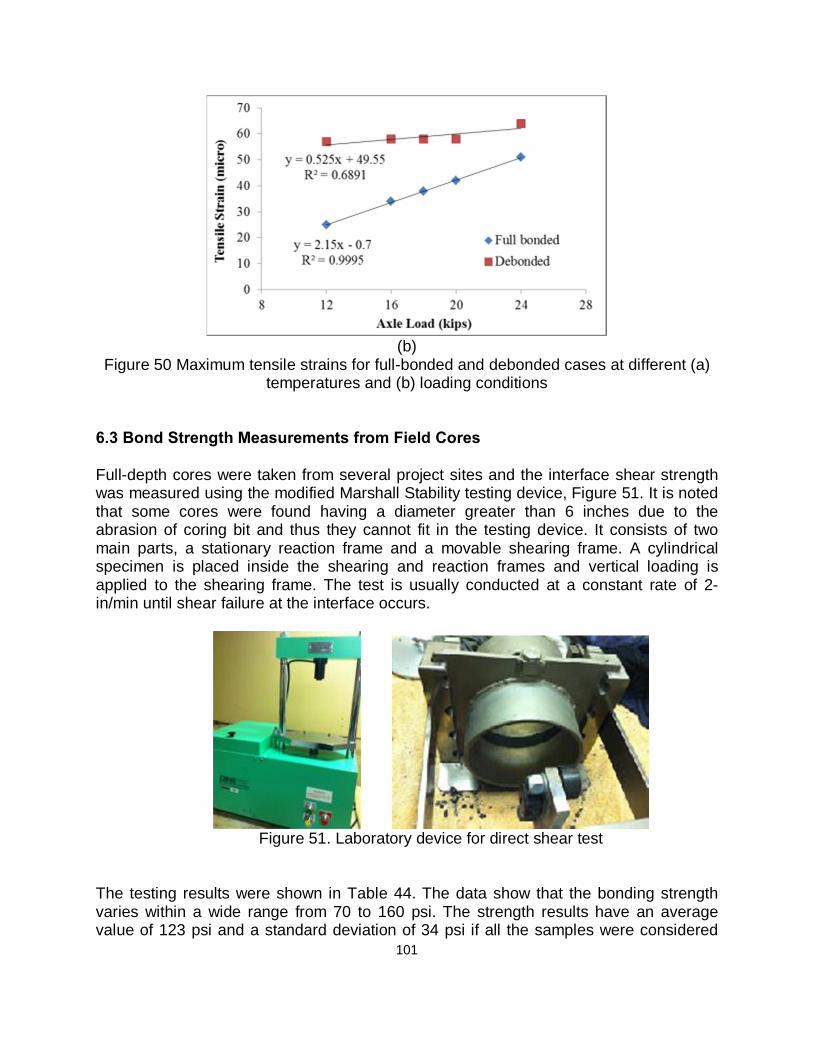
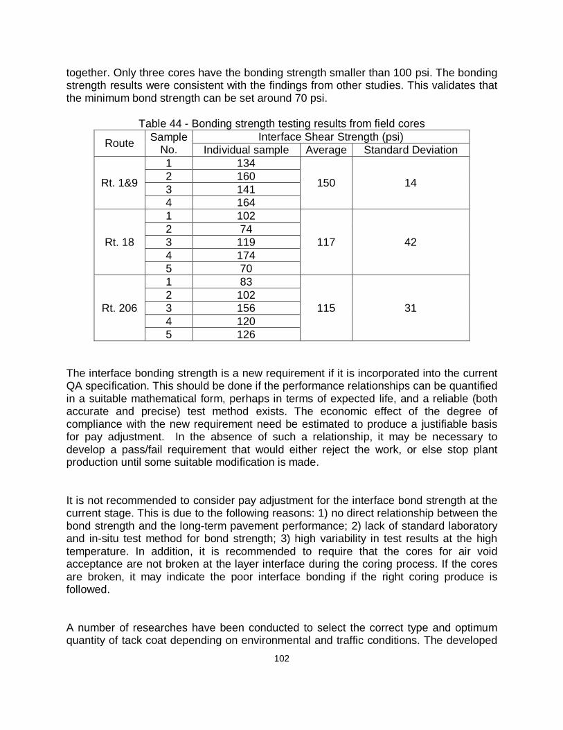
6. REQUIREMENT ON INTERFACE BONDING STRENGTH ..................................... 94 6.1 Importance of Interface Bonding on Pavement Life .................................... 94 6.2 Interface Shear Stress under Tire Loading................................................... 97 6.3 Bond Strength Measurements from Field Cores ....................................... 101

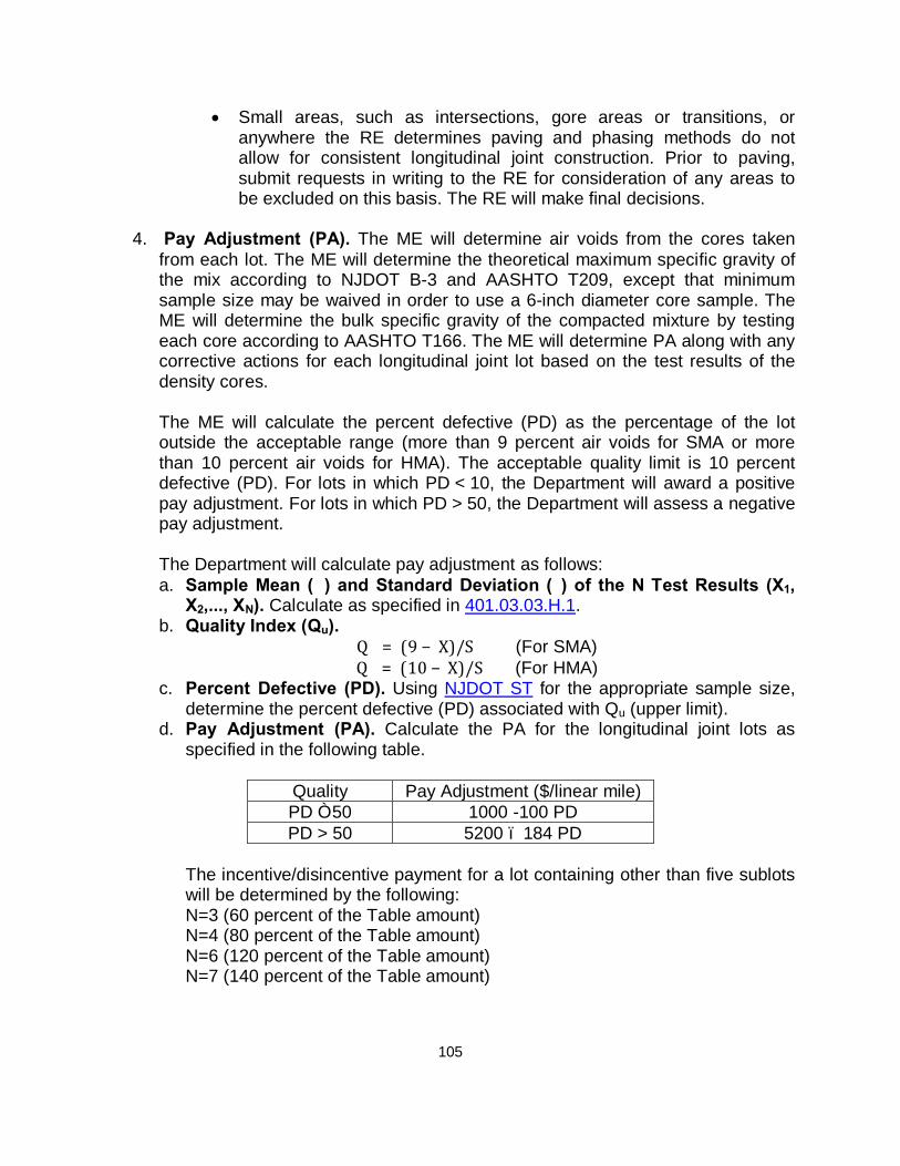
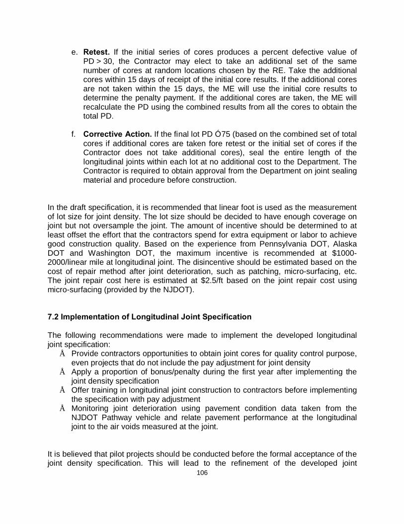
7. IMPLEMENTATION OF NEW SPECIFICATION .................................................... 104 7.1 Draft Longitudinal Joint Specification ........................................................ 104 7.2 Implementation of Longitudinal Joint Specification .................................. 106

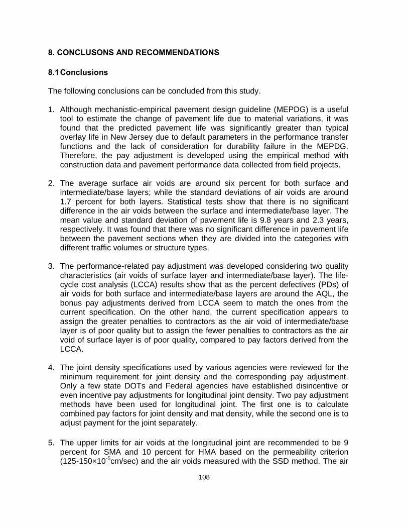
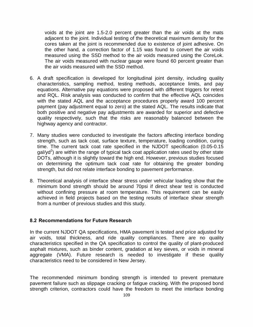
8. CONCLUSONS AND RECOMMENDATIONS ........................................................ 108 8.1 Conclusions .................................................................................................. 108 8.2 Recommendations for Future Research ..................................................... 109

9. REFERENCES ........................................................................................................ 111

iv

LIST OF FIGURES Page

Figure 1. Illustration of PD and PWL ...................................................................................14

Figure 2. Process of pavement performance prediction............................................... 24

Figure 3. Reliability of standard design and contractor’s construction (TxDOT Study) 27

Figure 4. Step-by-step processes to calculate pay factor (NCHRP 9-20) .................... 32

Figure 5. Illustration of predicted life difference and pay factors in QRSS (NCHRP 9-22)

.................................................................................................................................. 33

Figure 6. Illustration of taking joint cores (After Connecticut DOT specification) .......... 36

Figure 7. Interface shear testing devices: (a) direct shear fixture in Marshall Stability

tester, modified shear fixture with confinement at (b) Louisiana State University and

(c) University of Illinois at Urbana-Champaign; and (d) Superpave shear tester ....... 43

Figure 8. Torque test for interface bond strength ......................................................... 43

Figure 9. (a) University of Texas at El Paso pull-off device and (b) Louisiana tack coat

quality tester .............................................................................................................. 44

Figure 10. Interface bond strength for sites exhibited slippage failure (NCAT 2012) ... 52

Figure 11. Frequency distribution of (a) average air voids and (b) standard deviations

for surface layer for all construction lots .................................................................... 59

Figure 12. Frequency distributions of (a) average air voids and (b) standard deviations

for intermediate/base layer for all construction lots ................................................... 60

Figure 13. Frequency distributions of PDs of air voids of (a) surface layer and (b)

intermediate/base layer for all construction lots ........................................................ 62

Figure 14. Frequency distributions of PPAs of air voids of (a) surface layer and (b)

intermediate/base layer for all construction lots ........................................................ 63

Figure 15. Examples of SDI development trends for Rt. 45 and I-78 ........................... 64

Figure 16. SDI developments for all the sections ......................................................... 64

Figure 17. Examples of pavement performance deterioration models for construction

projects with different air voids .................................................................................. 65

Figure 18. Frequency distribution of pavement life for all the sections ........................ 66

Figure 19. Boxplot of pavement life for different traffic and structure conditions .......... 66

v

Figure 20. Corrleations between average air void contents of (a) surfac and (b)

intermediate layers and pavement life ....................................................................... 67

Figure 21. Corrleations between standard deviations of air void contents of (a) surfac

and (b) intermediate layers and pavement life .......................................................... 67

Figure 22. Illustration of exponential performance model with percent defectives ....... 69

Figure 23. Illustration of successive overlays due to premature pavement failure (77) 71

Figure 24. Comparison of pay adjustments when PDsurface AV=10 .......................... 72

Figure 25. Comparison of pay adjustments when PDintermediate AV=10 .................. 72

Figure 26. Pictures of (a) field coring and (b) nuclear gauge testing ............................ 75

Figure 27. Pictures of (a) field cores and (b) permeability testing device ..................... 76

Figure 28. Frequency distribution of air voids at the (a) joint and (b) mat .................... 77

Figure 29. Accumulative frequency distraction of air voids at the joint and mat ........... 78

Figure 30. Accumulative distributions of air voids at different offsets to joint ............... 78

Figure 31. (a) Theoretical maximum density values of cores taken from the mat and the

longitudinal joint and (b) air voids calculated using different theoretical maximum

density values ........................................................................................................... 79

Figure 32. Permeability and joint air voids measured with AASHTO T166 for (a) dense-

graded asphalt mixture and (b) stone-matrix asphalt ................................................ 81

Figure 33. Relationship between air voids measured using SSD method and CoreLok

.................................................................................................................................. 82

Figure 34. Relationship between air voids measured using SSD method and nuclear

gauge ........................................................................................................................ 82

Figure 35. Pay equations in SPECRISK analysis ........................................................ 84

Figure 36. SPECRISK analysis results for option 1 ..................................................... 86

Figure 37. Expected pay adjustment at different PDs (option 1) .................................. 87

Figure 38. Expected retest frequency at different PDs (option 1) ................................ 87

Figure 39. Expected frequency of corrective action at different PDs (option 1) ........... 88



Figure 42. OC curve for Retest frequency for Option A ............................................... 92

Figure 43. OC curve for RQL frequency for Option A .................................................. 92

vi

Figure 44. Composite pavement life for full-bonded and debonded cases with respect

to air voids of (a) surface layer and (b) intermediate layer ........................................ 96

Figure 45. Asphalt pavement life for full-bonded and debonded cases with respect to

air voids of (a) surface layer and (b) intermediate layer ............................................ 97

Figure 46. Illustration of (a) dual tires on AC overlay and (b) critical locations for

interface shear stress ................................................................................................ 98

Figure 47. Interface shear stresses at different interface depths ................................. 99

Figure 48. Interface shear stresses at different temperatures ...................................... 99

Figure 49. Interface shear stresses at different loading conditions ............................ 100

Figure 50 Maximum tensile strains for full-bonded and debonded cases at different (a)

temperatures and (b) loading conditions ................................................................. 101

Figure 51. Laboratory device for direct shear test ...................................................... 101

vii

LIST OF TABLES

Page Table 1 - Comparison of features of different construction specifications ..................... 10

Table 2 - Most Commonly used quality characteristics from NCHRP Synthesis 346 .... 12

Table 3 - Example of specification limits of quality characteristics (Delaware DOT) ..... 13

Table 4 - Description of different quality measures ....................................................... 15

Table 5 - Example of stepped (tabular) pay schedule (New York DOT) ........................ 17

Table 6 - Composite pay factor equations used by State agencies ............................... 18

Table 7 - Available test methods for HMA quality characteristics .................................. 23

Table 8 - Example of performance matrix for different PDs ........................................... 30

Table 9 - Mat and joint density specifications by different FEDEA ................................ 34

Table 10 - Literature review summary of pay adjustments for joint density ................... 35

Table 11 - Pay factors for mat and joint density in Connecticut ..................................... 37

Table 12 - Pay factors for mat and joint density in Kentucky ......................................... 37

Table 13 - Pay adjustment for joint density in Pennsylvania ......................................... 38

Table 14 - Pay factors for joint density in Federal Aviation Administration .................... 40

Table 15 - Pay factors for mat and joint density in US Army ......................................... 41

Table 16 - Testing matrix for bond strength (NCHRP 9-40) ........................................... 45

Table 17 - Bond strength testing results for different surface types and preparation

methods (NCHRP 9-40) .......................................................................................... 45

Table 18 - Comparison of bond strength and interface shear stress (NCHRP 9-40) ..... 46

Table 19 - Testing matrix for bond strength (Illinois DOT Study) ................................... 47

Table 20 - Effect of tack coat rate and surface texture on bond strength ...................... 47

Table 21 - Effect of temperature effect on bond strength (ICT Study) ........................... 47

Table 22 - Effect of mixture type on bond strength (Illinois DOT Study) ........................ 48

Table 23 - Effect of curing time and tack coat material on bond strength ...................... 48

Table 24 - Bond strength of field cores on I-80 (Illinois DOT Study).............................. 48

Table 25 - Bond strengths of laboratory-prepared samples for (a) CRS-2 (b) CSS-1; and

(c) PG64-22 (NCAT Study) ..................................................................................... 49

Table 26 - Bond strength results for of field cored specimen (NCAT Study) ................. 51

viii

Table 27 - Testing matrix for bond strength (Study in Italy) ........................................... 52

Table 28 - Comparison the shear stress between Ancona shear device and layer-

parallel direct shear device (Study in Italy) ............................................................. 53

Table 29 - Bond strength using field cores with short curing time (Study in Italy) ......... 53

Table 30 - Bond strength using field cores with medium curing time (Study in Italy) ..... 54

Table 31 - Effect of displacement rate and temperature on bond strength (FLDOT Study)

................................................................................................................................ 54

Table 32 - Bond Strength using field cores on I-90 (FLDOT Study) .............................. 55

Table 33 - Testing matrix for bond strength (Louisiana DOTD Study) ........................... 55

Table 34 - Effect of normal stress and temperature on bond strength (Louisiana DOTD

Study) ..................................................................................................................... 56

Table 35 - Air voids requirements in the NJDOT specification ...................................... 61

Table 36 - Rational check of pavement performance model with PDs .......................... 69

Table 37 - Summary of field cores for joint air void study .............................................. 74

Table 38 - Gradations of asphalt mixtures used at field projects ................................... 75

Table 39 - Volumetric properties of asphalt mixtures used at field projects................... 76

Table 40 - Summary of features and performance of options A, B, and C .................... 91

Table 41 - Pavement structures used for debonding analysis ....................................... 94

Table 42 - Failure criteria for pavement life prediction ................................................... 95

Table 43 - Parameter ranges considered in interface stress analysis ........................... 98

Table 44 - Bonding strength testing results from field cores ........................................ 102

ix

LIST OF ABBREVIATIONS AND SYMBOLS AADTT - Annual Average Daily Truck Traffic

AASHTO - American Association of State Highway and Transportation Officials

AC - Asphalt Concrete

AQL - Acceptable Quality Level

AV - Air Void

DOT - Department of Transportation

ESAL - Equivalent Single Axle Load

FAA - Federal Aviation Administration

FHWA - Federal Highway Administration

Gmm - Theoretical Maximum Specific Gravity

HMA – Hot-Mix Asphalt

IRI - International Roughness Index

JMF - Job Mix Formula

LCC - Life Cycle Cost

LCCA – Life-Cycle Cost Analysis

MEPDG - Mechanistic-Empirical Pavement Design Guide

NCAT - National Center for Asphalt Technology

NCHRP - National Cooperative Highway Research Program

NDT - Non-Destructive Testing

NJDOT – New Jersey Department of Transportation

NMAS - Nominal Maximum Aggregate Size

NPV - Net Presence Value

OC - Operating Characteristic

PAM - Percent Above Minimum

PPA - Percent Pay Adjustment

PCC - Portland Cement Concrete

PG - Performance Grade

PMS – Pavement Management System

PF - Pay Factor

x

PD - Percent Defective

PWL - Percent Within Limit

PSI - Present Serviceability Index

PRS - Performance-Related Specification

QA - Quality Assurance

QC - Quality Control

QRSS – Quality-Related Specification Software

RQL - Rejectable Quality Level

SDI - Surface Distress Index

SSD - Saturated Surface Dry

SMA - Stone Matrix Asphalt

TCC - Truck Traffic Classification

TMD - Theoretical Maximum Density

VMA - Voids in Mineral Aggregate

1

1. EXECUTIVE SUMMARY It is strongly desired by agencies to develop a simple but scientifically based pay adjustment methodology that is practical and effective, fair to both the highway agency and the construction industry, and legally defensible. Therefore, pay factors due to material and/or construction variations in the as-constructed pavements should be developed to reflect expenses or savings expected to occur in the future as the result of a departure from the specified level of pavement quality. The objective of New Jersey Department of Transportation (NJDOT) 2012-01 project, HMA Pay Adjustment, is to critically evaluate how multiple quality characteristics of HMA can best be incorporated into pay adjustment and develop performance-related pay adjustment for the NJDOT. Pay Adjustment for In-Place Air Void An extensive literature review was conducted to review previous research studies related to the project objective. The literature review covers four main topics:

• Evolution of pavement construction specifications; • Statistically-based acceptance produce; • HMA quality characteristics and test methods; and • State-of-practice on performance-related pay adjustment.

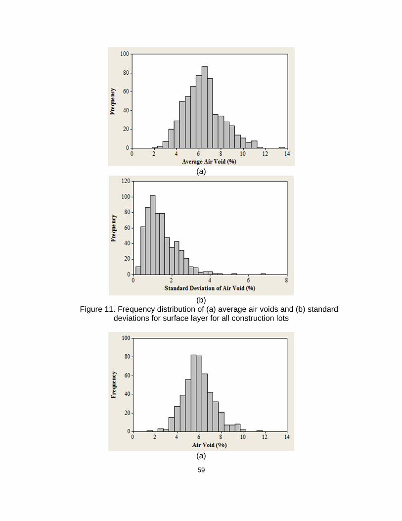
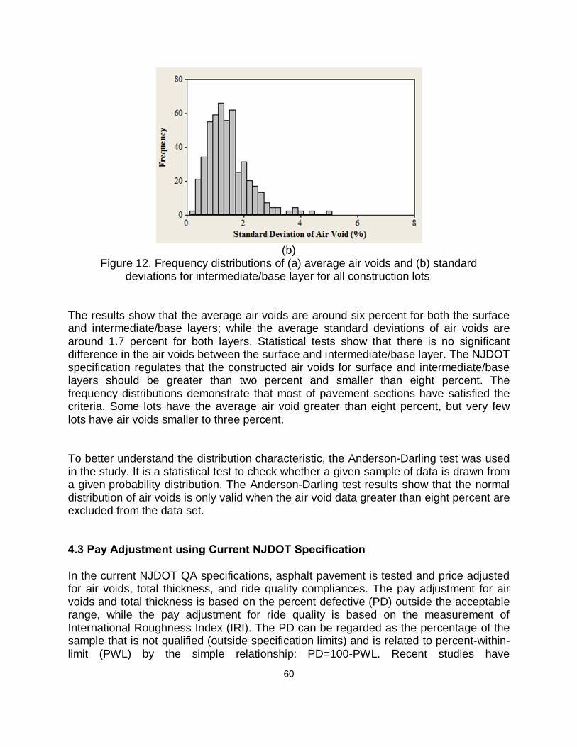
In-place air void data were collected from quality assurance records for a large number of projects constructed in New Jersey from 1995 to 2005. Pavement condition data were extracted from pavement management system (PMS). The data show that the average surface air voids are around six percent for both surface and intermediate/base layers; while the standard deviations of air voids are around 1.7 percent for both layers. Empirical pavement performance models were developed with sigmoidal functions and used to predict pavement service life. The mean value and standard deviation of pavement life was found equal to 9.8 years and 2.3 years, respectively. An exponential model form was used to relate the expected pavement service life to the quality measures of in-place air voids. The performance-related pay adjustment was developed using the life-cycle cost analysis (LCCA). The results show that as the percent defectives (PDs) of air voids for both surface and intermediate/base layers are around the acceptable quality level (AQL), the bonus pay adjustments derived from LCCA seem to match the ones from the current specification. On the other hand, the current specification appears to assign greater penalties to contractors for the air void if intermediate/base layer is of poor quality but to assign lesser penalties to contractors for the air void if surface layer is of poor quality, as compared to pay factors derived from the LCCA.

2

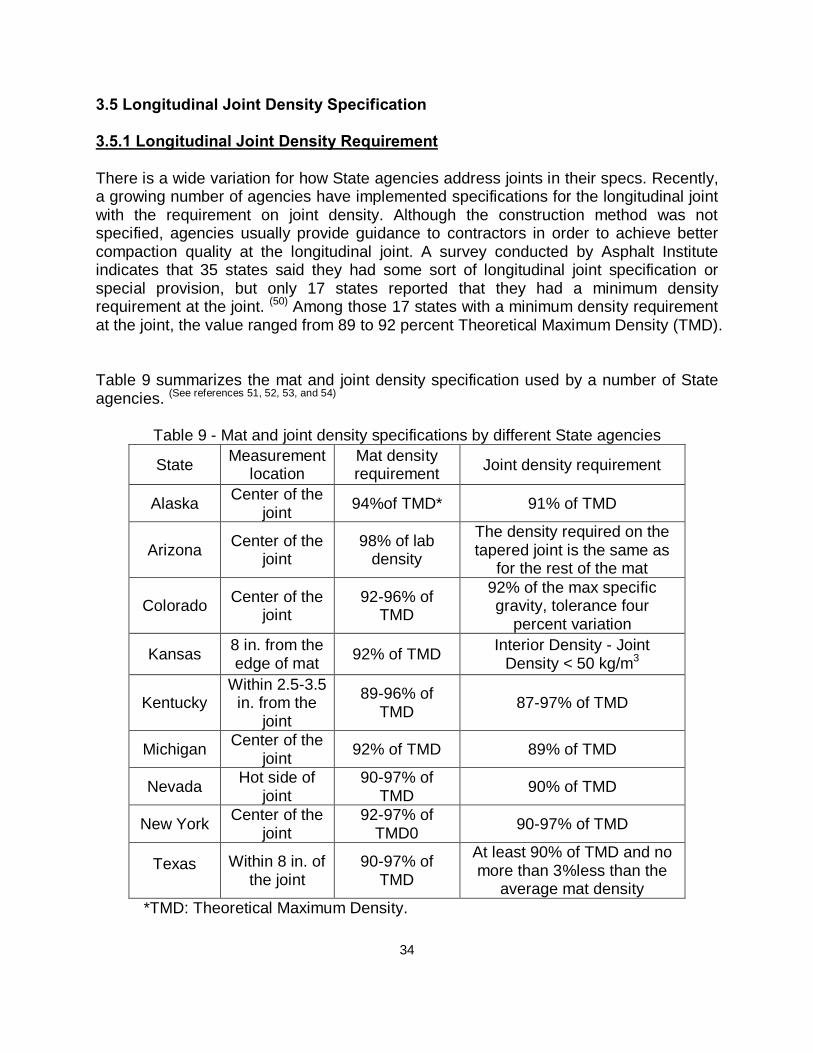
Pay Adjustment for Air Void at Longitudinal Joint The existing joint density specifications used by various agencies were reviewed for the minimum requirement for joint density and the corresponding pay adjustment. The following findings were concluded from the review:

• Most agencies use cores to measure the joint density. • The majority of agencies measure the joint density at the center of longitudinal

joint. Other agencies may measure the joint density within three to eight inches away from the joint.

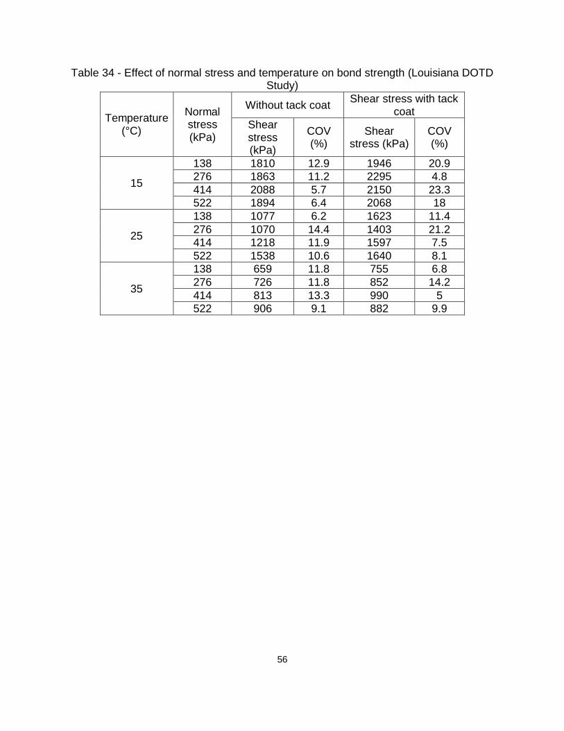
• The requirements for the joint density are usually two to three percent below the requirements for the mat density. Most agencies specify that the joint density should be above 89 to 90 percent of theoretical maximum density (TMD).

• Two pay adjustment methods have been used for longitudinal joint. The first one is to calculate combined pay factors for joint density and mat density, while the second one is to adjust payment for the joint separately.

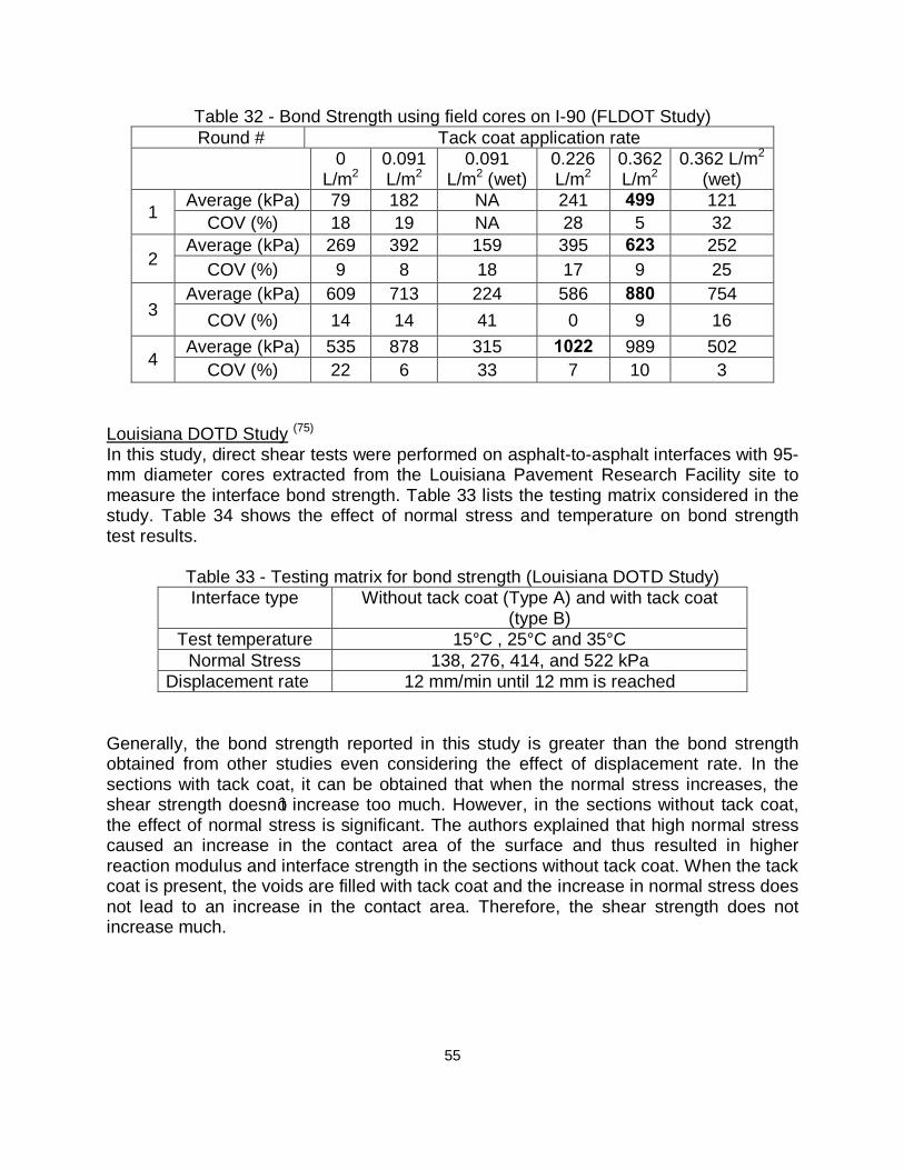
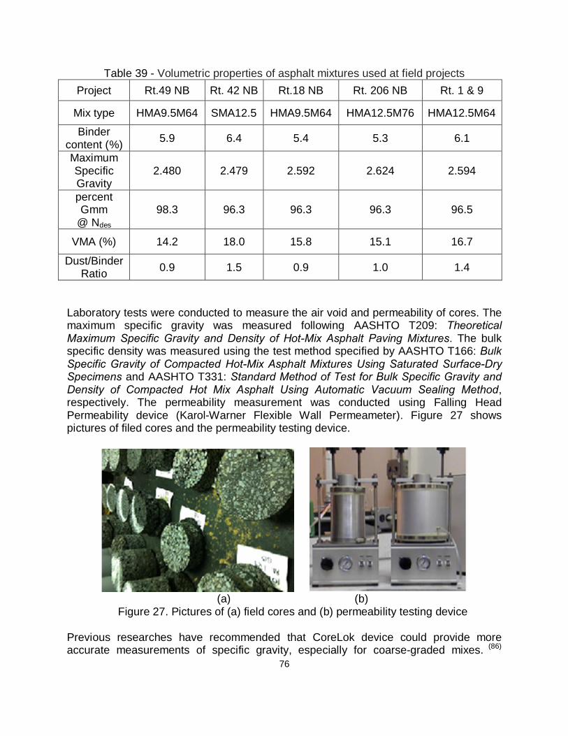
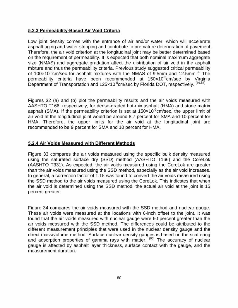
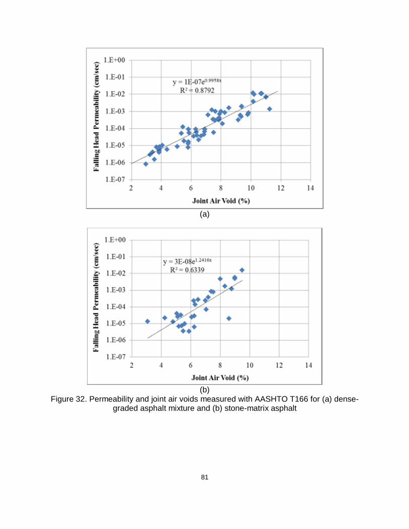
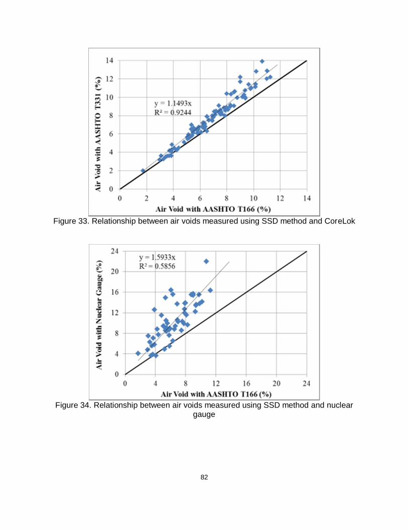
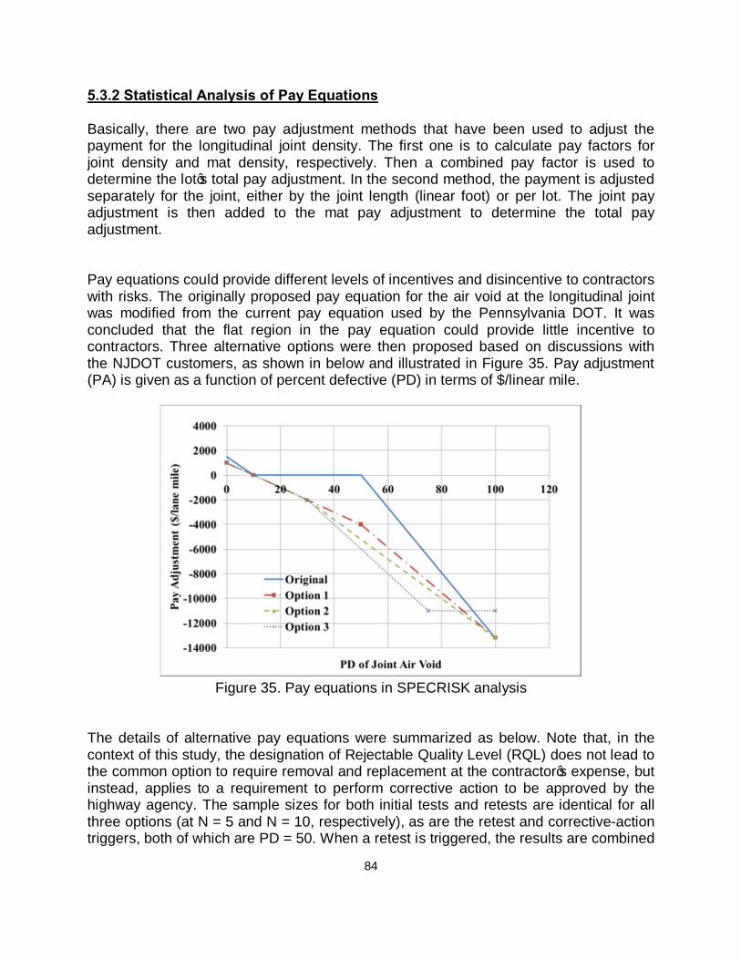
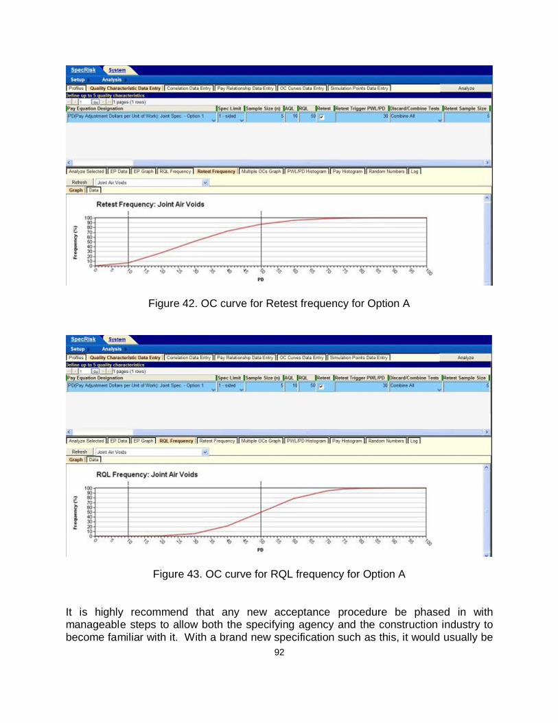
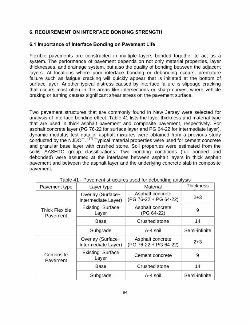
Laboratory tests were conducted to measure air voids of field cores using the saturated surface dry (SSD) method (AASHTO T166) and the automatic vacuum sealing method (AASHTO T331). The permeability measurement was conducted using Falling Head Permeability device. The air voids at the joint were found 1.5-2.0 percent greater than the air voids at the mats adjacent to the joint. Individual testing of the theoretical maximum density for the cores taken at the joint is recommended due to existence of joint adhesive. The upper limits for air voids at the longitudinal joint are recommended to be nine percent for SMA and 10 percent for HMA based on the permeability criterion (125-150×10-5cm/sec) and air voids measured with the SSD method. Alternative pay equations for air voids at the longitudinal joint were proposed with different triggers for retest and acceptable quality level (AQL). SPECRISK analysis was conducted to confirm that the effective AQL coincides with the stated AQL and the acceptance procedures properly award 100 percent payment (pay adjustment equal to zero) at the stated AQL. Finally, a draft specification for longitudinal joint density is developed with suggestions for future implementation and training. The specification includes quality characteristics, sampling method, testing methods, acceptance limits, and pay equations.

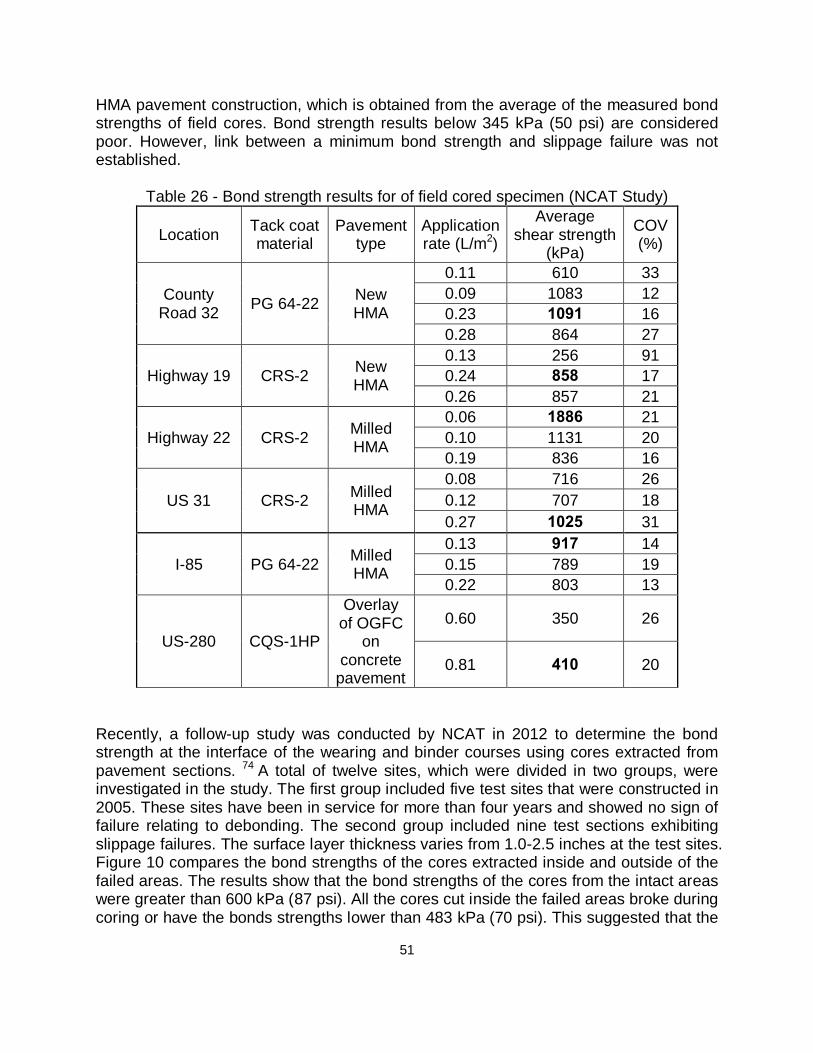
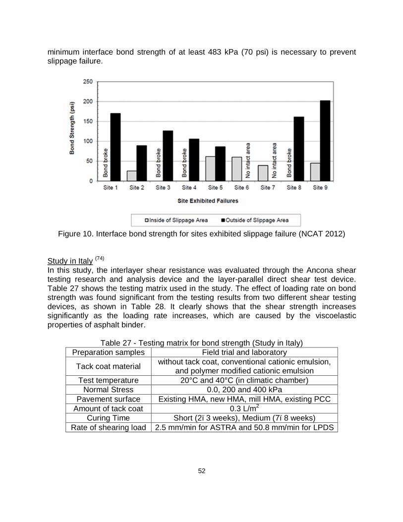
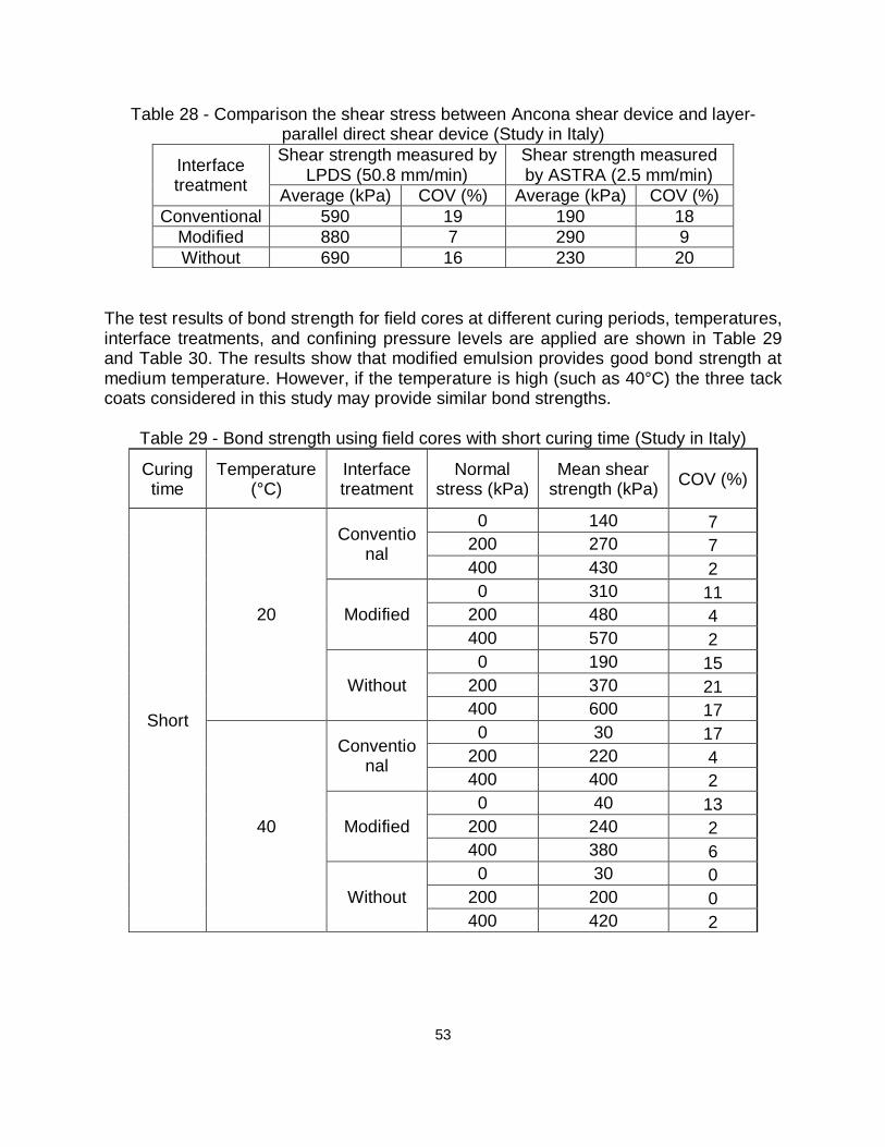
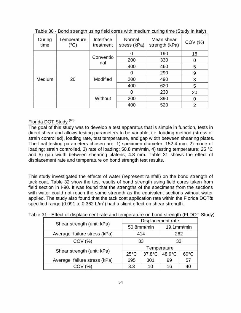
Interface Bonding Strength Over the years, a number of studies have been conducted to investigate the actual interface bond strength in field conditions and the factors that affect interface bonding strength between asphalt layers. The general conclusions summarized from the literature review are as follows:

3

• Most studies focused on the factors affecting interface bonding strength and the optimum tack coat application rate, while few studies studied the minimum bonding strength required to avoid premature pavement failure.

• The bond strength testing results varied depending on test conditions. It can be concluded that the lower temperature, higher normal pressure, and higher displacement rate during testing can significantly increase bond strength.

• The optimum tack coat application rates to achieve the maximum bond strength were found varying in different ranges depending on tack coat type and surface condition.

• Laboratory-prepared samples usually resulted in the greater bond strength when compared to field cores. This is probably because the higher compaction level is achieved in the laboratory and the deterioration of pavement exists at field.

Pavement structural analysis was conducted to predict the interface shear stress between the surface and intermediate asphalt layers under the combination of vertical and horizontal loading at different temperatures. Theoretical analysis results show that the minimum bond strength requirement should be around 70psi (direct shear test without confining pressure at room temperature) in order to prevent premature pavement failure such as slippage cracking or fatigue cracking. This requirement can be easily achieved in field projects based on the testing results of bond strength from a number of previous studies and this study.

Recommendations for Future Research In the current NJDOT specifications, HMA pavement is tested and price adjusted for air voids, total thickness (new or reconstruction only), and ride quality compliances. There are no quality characteristics specified in the quality assurance (QA) specification to control the quality of plant-produced asphalt mixtures, such as binder content, gradation at key sieves, or voids in mineral aggregate (VMA). Future research is needed to investigate if these quality characteristics need to be considered in New Jersey. With the proposed bond strength criterion, contractors could have the freedom to meet interface bonding requirement with cost-effective procedures and techniques instead of following the required tack coat type and application rate. Future research is recommended to investigate the relationship between interface bonding and the expected pavement life so an appropriate pay adjustment could be developed. This will eventually lead to the development of performance-related specifications for interface bonding requirement. The new acceptance procedure on longitudinal joint density needs to be phased in with manageable steps to allow both the NJDOT and the construction industry to become familiar with it. Pilot projects are recommended before its full implementation. The

4

proposed pay equations should be refined and validated with field performance data through long-term monitoring.

5

2. INTRODUCTION 2.1 Background Quality assurance (QA) specifications and acceptance procedures have been widely used by state highway agencies to improve the performance of constructed pavements and reduce maintenance costs. These procedures typically specify an end result that can be measured in statistical terms and award payment in proportion to the extent to which the end result has been achieved. The intent of the pay-adjustment approach is twofold - to encourage contractors to deliver the desired level of quality (or better) and, failing that, to recoup for the highway agency the potentially substantial future costs that will likely result from deficient quality. In the current NJDOT specifications, hot-mix asphalt (HMA) pavement is tested and price adjusted for in-place air voids, total thickness, and ride quality compliances. (1) The pay adjustment for in-place air voids and total thickness is based on the percent defective (PD) outside the acceptable range, while the pay adjustment for ride quality is based on the average smoothness value. The current pay factors in the NJDOT specifications are based on empirical field data and engineering experience to estimate the economic impact on the highway agency of either a shortening or an extension of expected design life. (2) As such, they are believed to fairly award contractors for providing work that equals or exceeds the acceptable quality level, and also to fairly recoup expected future expenses resulting from substandard work. It is desired that the pay-adjustment procedures used by State agencies should be designed to reflect expenses or savings expected to occur in the future as the result of a departure from the specified level of pavement quality, and have been patterned after the legal principle of liquidated damages. Therefore, the logical and defensible method to develop pay adjustments is based on the difference between the life-cycle-cost value of the as-constructed pavement and that of the as-designed pavement. However, it is recognized that this approach can become complex due to the uncertainty of maintenance and rehabilitation schedules used by highway agencies, and also due to possible correlation and interaction among the various quality characteristics. (3) This study will develop simple but scientifically based pay adjustments for in-place air voids and validate with pavement performance data. A number of states have begun to implement longitudinal joint specifications, and most are based on determinations of density (e.g. New York DOT requires 90 percent and Federal Aviation Administration (FAA) requires 93.3 percent minimum joint density). However, distress at the joint is caused by the ability of air and water to enter the pavement structure, which is also related to permeability. (4) This study will recommend the specification limits for air voids at the longitudinal joint based on density and

6

permeability testing results. Before the new specification for longitudinal joint is implemented for field application, the standard procedure is to assess the risks to both the highway agency and the construction industry. If any such risks are found to be too large, the specification can be revised and reanalyzed. Therefore, risk analysis of the proposed pay equations for longitudinal joint quality will be conducted. It has been proven that the interface bonding between pavement layers is critical to avoid premature pavement failure and ensure long-term performance, especially for pavement overlays. However, the requirement on interface bonding strength has not been specified in the construction specification before. The interface bonding between asphalt layers are affected by many factors, such as tack coat type and rate, surface roughness, and testing conditions. The interface failure potential increases when a significant amount of horizontal shear stress is applied on pavement surface due to vehicle braking and acceleration. Therefore, analysis is needed to determine the minimum requirement of interface bonding strength to withstand the interface stress caused by vehicular loading. 2.2 Objective The objectives of this research are to

1) Develop a performance-related pay adjustment methodology for in-place air void; 2) Develop a specification for longitudinal joint density; and 3) Determine the minimum requirement on interface bonding strength between

asphalt layers.

7

3. LITERATURE REVIEW 3.1 Review of Specifications for Pavement Construction There are six basic types of specifications for pavement construction, including method specification, end-result specification, quality assurance specification, performance related specification, performance-based specification, and warranty. The following sections describe the details of each type of construction specification.(5,6) Method Specification As an original construction specification, Method Specifications can also be called Material Specifications, Recipe Specifications or Prescriptive Specifications. It was widely used in 1940 and served their purpose well in the highway construction and are still used by local agencies of small towns or counties. In Method Specifications, the contractor are required to produce and place a pavement product using specified materials, certain types of equipment and methods under the guidance of the agency. In other words, the contractor’s role is to lend its workers and equipment to the agency. If the contractor follows the procedures, or “recipe,” they can receive full payment for the constructed pavement. As the original construction specification, it is relatively simple and many problems are ignorable when compared to other construction specifications. First, under this circumstance, the contractor cannot use innovative or economical solutions since their operation is fixed by the agency; Second, the risk basically transfers to the agency once the construction is failed; Third, contractor has no incentive to improve product quality and achieve better construction performance because there is no bonus when their product has outstanding performance; Fourth, the materials acceptance is based on the test result of individual field samples selected by the agency that ignores the inherent variability in construction materials. Five, the payment is not correlated to long-term pavement performance. End-Result Specification End-Result Specifications require the contractor to take the whole responsibility for producing and placing the product while the agency’s responsibility is to judge the final product: either accepts or rejects the final product, or implements a penalty system that calculates the degree of non-compliance. Compared to Method Specifications, this type of specification focuses on final product quality rather than procedure. The risk for the agency decreases and it mainly depends on the acceptance limits and processes used by the agency. The specification affords the contractor a large amount of freedom in developing innovative procedures and techniques to reduce the cost and perform the work. The price adjustment is based on the degree of compliance with the specification, which stimulates contractors to improve the quality of end product.

8

The main disadvantage of End-Result Specifications is that the acceptance decisions are limited to the few results from in-place testing and may still reject acceptable material. The specification acceptance values are subjective or empirical. Thus the relationship between the measured quality characteristics and final pavement performance may be nebulous. Quality Assurance Specification Quality Assurance Specifications began in 1960’s and it is a popular specification nowadays. It was derived from U.S. Department of Defense specifications (Military Standard 414 – Sampling Procedures and Tables for Inspection by Variables for Percent Defective). As statistically-based specifications, it includes quality control by contractor and acceptance activities by agency in the production process. The Quality Assurance Specification is also called quality assurance / quality control (QA/QC) specification. It combines End-Result Specifications and Method Specifications. In order to produce a pavement product which can pass the specifications stipulated by the highway agency, the contractor keeps implementing the quality control to adjust the production. The highway agency identifies the specific quality characteristics to be evaluated for quality acceptance (sampling, testing, and inspection). Through the result from acceptance by agency, the price adjustments related to quality level of the final product is decided. Generally, final acceptance uses multiple measurements within an entire lot (random sampling and lot-by-lot testing) rather than individual measurements. Final acceptance of the product is usually based on a statistical sampling of the measured quality level for key quality characteristics. The quality level is typically presented in statistical terms such as the mean and standard deviation, percent within limits, average absolute, etc. The statistical probability approach is normally used to increase the precision of the test and reduce both the buyer’s risk and the seller’s risk. In the current Quality Assurance Specifications used by most states, for superior quality product, the contractor may receive bonus payment typically one to five percent of the bid price; contractor with low quality work will receive zero to 99 percent reduced payment or the product may even be rejected by the agency. Performance-Related Specification After the 1980’s, some transportation agencies started to investigate a specification that can correlate construction quality to long-term performance. In fact, Performance-Related Specifications are improved Quality Assurance Specifications that use Life Cycle Cost Analysis (LCCA) to relate the quality characteristics, pavement performance, and pay adjustment. Compared to Quality Assurance Specifications which only measure the instantaneous quality characteristics after construction, Performance-Related Specifications focus more on long-term product performance. The pay adjustment in Quality Assurance Specifications is usually empirical and relatively simple while it is more complicated in Performance-Related Specifications. Performance-

9

Related Specifications may build a model that considers multiple material and construction quality characteristics (such as air void and layer thickness), design variables (such as traffic, climate, structural conditions), and pavement performance indicators (such as roughness and multiple distresses) to calculate the LCC and adjust the payment. To develop Performance-Related Specifications, the reliable performance-prediction models and maintenance-cost models are needed. Although several research studies have been conducted by the FHWA and NCHRP, only few agencies implement it into the real practice due to lack of agency specific data. Performance-Based Specification Performance-Based Specifications are developing specifications. Transportation Research Circular Number E-C037 defines Performance-Based Specifications as: Quality Assurance Specifications that describe the desired levels of fundamental engineering properties that are primary predictors of performance. The Performance-Based Specifications are different from Performance-Related Specifications primarily in the indicators they use to predict the performance. Performance-Based Specifications focus on resilient modulus, creep properties, fatigue, and other properties that can be used to predict pavement response, distress, or performance under different traffic, climate and structural conditions. To implement Performance-Based Specifications, the performance-based test methods and the mathematical models to predict pavement performance and costs are needed. Currently, performance-based test methods for measuring fundamental engineering properties have not been fully developed and some methods that have been developed are not yet user-friendly enough to permit timely acceptance testing in daily construction practice. Warranty Warranty is another type of specification that focuses on long-term pavement performance. The difference is that it measures performance indicators after one to ten years of construction. The warranty specification contains thresholds for different pavement distresses, which are usually developed from performance data in the pavement management system database by using statistical analysis and expert opinions. For example, in the warranty specification developed by the Wisconsin DOT in 2000, if a distress threshold is reached within five years (such as one percent alligator cracking in the area of a pavement segment), the contractor is responsible for conducting the remedial (corrective) action as specified in the Warranty. Under the Warranty, the contractors are encouraged to use innovative practices to provide longer-lasting pavements. With short-term warranties, the quality responsibility is shifted to the contractor thereby decreasing the agency’s risk.

10

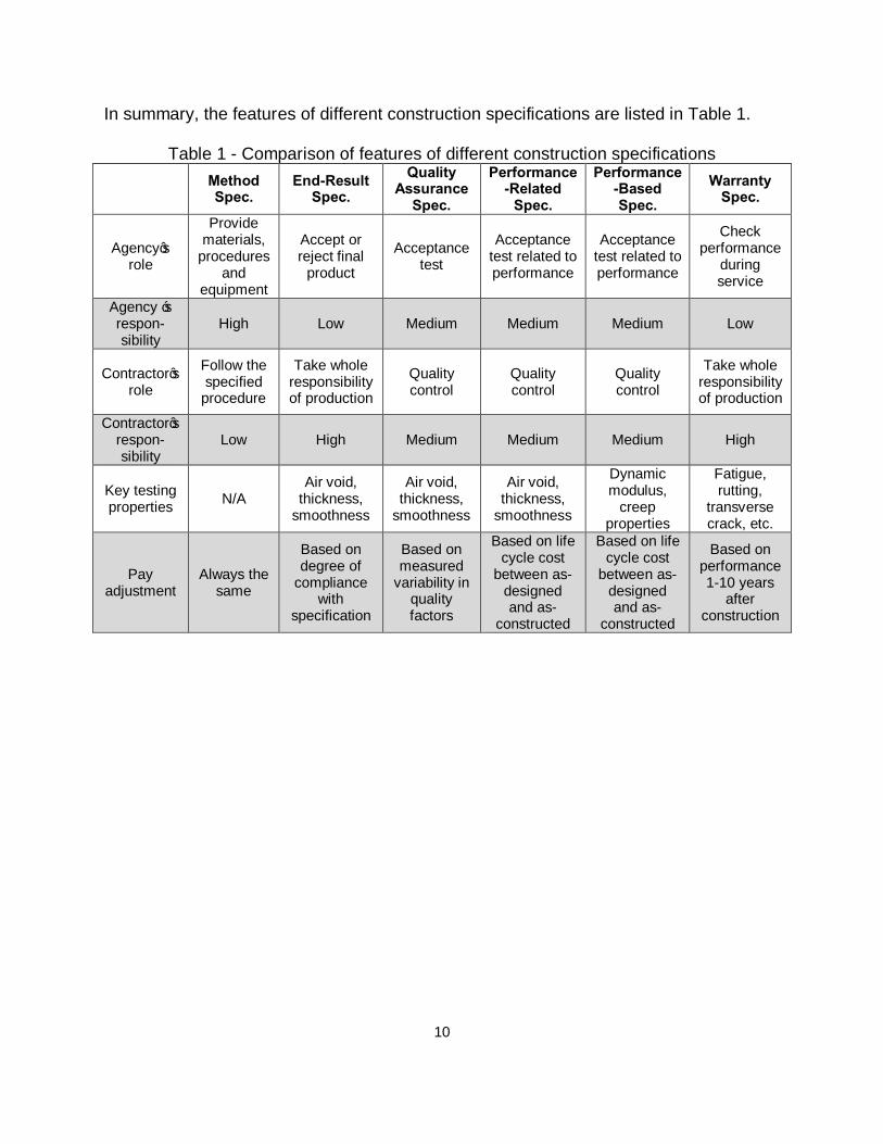
In summary, the features of different construction specifications are listed in Table 1.

Table 1 - Comparison of features of different construction specifications

Method Spec.

End-Result Spec.

Quality Assurance

Spec.

Performance-Related

Spec.

Performance-Based Spec.

Warranty Spec.

Agency’s role

Provide materials,

procedures and

equipment

Accept or reject final

product

Acceptance test

Acceptance test related to performance

Acceptance test related to performance

Check performance

during service

Agency ‘s respon-sibility

High Low Medium Medium Medium Low

Contractor’s role

Follow the specified

procedure

Take whole responsibility of production

Quality control

Quality control

Quality control

Take whole responsibility of production

Contractor’s respon-sibility

Low High Medium Medium Medium High

Key testing properties N/A

Air void, thickness,

smoothness


smoothness


smoothness

Dynamic modulus,

creep properties

Fatigue, rutting,

transverse crack, etc.

Pay adjustment

Always the same

Based on degree of

compliance with

specification

Based on measured

variability in quality factors

Based on life cycle cost

between as-designed and as-

constructed

Based on life cycle cost

between as-designed and as-

constructed

Based on performance 1-10 years

after construction

11

3.2 Acceptance Procedure and Pay Factors Quality Assurance (QA) Specifications are widely implemented into pavement construction nowadays. An important aspect of the QA specification is the acceptance procedure. Acceptance procedure is not a method to control or improve pavement quality, like quality control (QC). Instead, it is used to define whether the final product should be accepted, rejected, or accepted at a reduced payment. QA acceptance plans are being used or developed by about 90 percent of state highway agencies and most Federal transportation agencies. In the acceptance plan, pay factors are developed based on the quality measure of certain quality characteristics compared to the specific specification limits. The following components provide a basis for the statistically-based acceptance procedure in QA. (7)

(1) Acceptance Sampling; (2) Quality Characteristics; (3) Specification Limits; (4) Quality Measure; (5) Acceptance Limits; (6) Pay Factors; (7) Risk;

3.2.1 Acceptance Sampling Acceptance sampling is typically used in quality acceptance for pavement construction. It uses a small number of random samples to draw conclusions about a large amount of material (called a “lot”). Acceptance sampling always follows two basic concepts to achieve effectiveness: estimation of material properties and random sampling. For pavement construction, stratified random sampling, which involves dividing lots into several equal-sized sublots, is generally used.(8) There are two types of acceptance sampling: attribute sampling and variable sampling. Attribute sampling inspects whether specific attributes are qualified in a sample. Then a simple record with passing or failing is made according to the standard. For example, aggregate is accepted or rejected based on a specified minimum percentage of one fractured face. The actual percentage of fractured face is not recorded; instead, a simple pass or fail record is used. In variable sampling, the measurement values are retained as continuous variables rather than converted into simple record. Most variable sampling plans assume a normal distribution of the measured property, which is usually true for construction-related quality characteristics such as pavement material properties. Since variable sampling records more information from samples, it is more commonly used in the statistical acceptance plans.

12

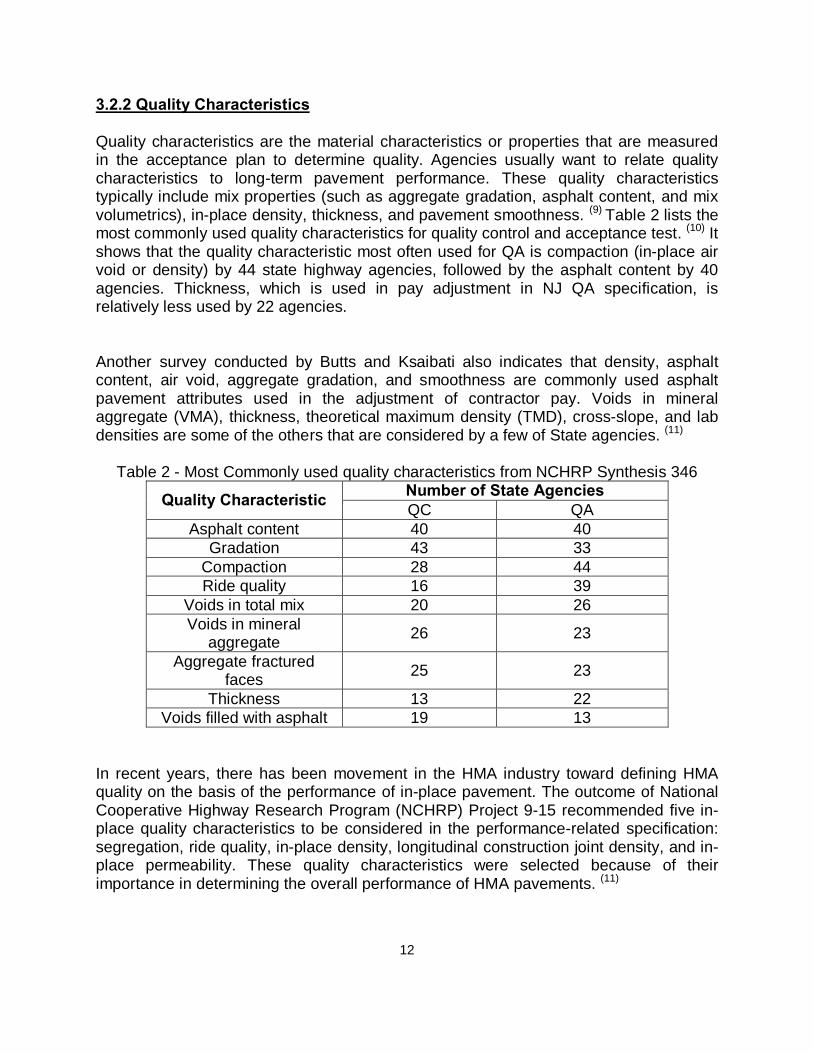
3.2.2 Quality Characteristics Quality characteristics are the material characteristics or properties that are measured in the acceptance plan to determine quality. Agencies usually want to relate quality characteristics to long-term pavement performance. These quality characteristics typically include mix properties (such as aggregate gradation, asphalt content, and mix volumetrics), in-place density, thickness, and pavement smoothness. (9) Table 2 lists the most commonly used quality characteristics for quality control and acceptance test. (10) It shows that the quality characteristic most often used for QA is compaction (in-place air void or density) by 44 state highway agencies, followed by the asphalt content by 40 agencies. Thickness, which is used in pay adjustment in NJ QA specification, is relatively less used by 22 agencies. Another survey conducted by Butts and Ksaibati also indicates that density, asphalt content, air void, aggregate gradation, and smoothness are commonly used asphalt pavement attributes used in the adjustment of contractor pay. Voids in mineral aggregate (VMA), thickness, theoretical maximum density (TMD), cross-slope, and lab densities are some of the others that are considered by a few of State agencies. (11)

Table 2 - Most Commonly used quality characteristics from NCHRP Synthesis 346

Quality Characteristic Number of State Agencies QC QA

Asphalt content 40 40 Gradation 43 33

Compaction 28 44 Ride quality 16 39

Voids in total mix 20 26 Voids in mineral

aggregate 26 23

Aggregate fractured faces 25 23

Thickness 13 22 Voids filled with asphalt 19 13

In recent years, there has been movement in the HMA industry toward defining HMA quality on the basis of the performance of in-place pavement. The outcome of National Cooperative Highway Research Program (NCHRP) Project 9-15 recommended five in-place quality characteristics to be considered in the performance-related specification: segregation, ride quality, in-place density, longitudinal construction joint density, and in-place permeability. These quality characteristics were selected because of their importance in determining the overall performance of HMA pavements. (11)

13

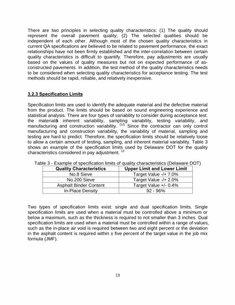
There are two principles in selecting quality characteristics: (1) The quality should represent the overall pavement quality; (2) The selected qualities should be independent of each other. Although most of the chosen quality characteristics in current QA specifications are believed to be related to pavement performance, the exact relationships have not been firmly established and the inter-correlation between certain quality characteristics is difficult to quantify. Therefore, pay adjustments are usually based on the values of quality measures but not on expected performance of as-constructed pavements. In addition, the test method of the quality characteristics needs to be considered when selecting quality characteristics for acceptance testing. The test methods should be rapid, reliable, and relatively inexpensive. 3.2.3 Specification Limits Specification limits are used to identify the adequate material and the defective material from the product. The limits should be based on sound engineering experience and statistical analysis. There are four types of variability to consider during acceptance test: the material’s inherent variability, sampling variability, testing variability, and manufacturing and construction variability. (12) Since the contractor can only control manufacturing and construction variability, the variability of material, sampling and testing are hard to predict. Therefore, the specification limits should be relatively loose to allow a certain amount of testing, sampling, and inherent material variability. Table 3 shows an example of the specification limits used by Delaware DOT for the quality characteristics considered in pay adjustment. 13

Table 3 - Example of specification limits of quality characteristics (Delaware DOT) Quality Characteristics Upper Limit and Lower Limit

No.8 Sieve Target Value -/+ 7.0% No.200 Sieve Target Value -/+ 2.0%

Asphalt Binder Content Target Value +/- 0.4% In-Place Density 92 - 96%

Two types of specification limits exist: single and dual specification limits. Single specification limits are used when a material must be controlled above a minimum or below a maximum, such as the thickness is required to not smaller than 3 inches. Dual specification limits are used when a material must be controlled within a range of values, such as the in-place air void is required between two and eight percent or the deviation in the asphalt content is required within ± five percent of the target value in the job mix formula (JMF).

14

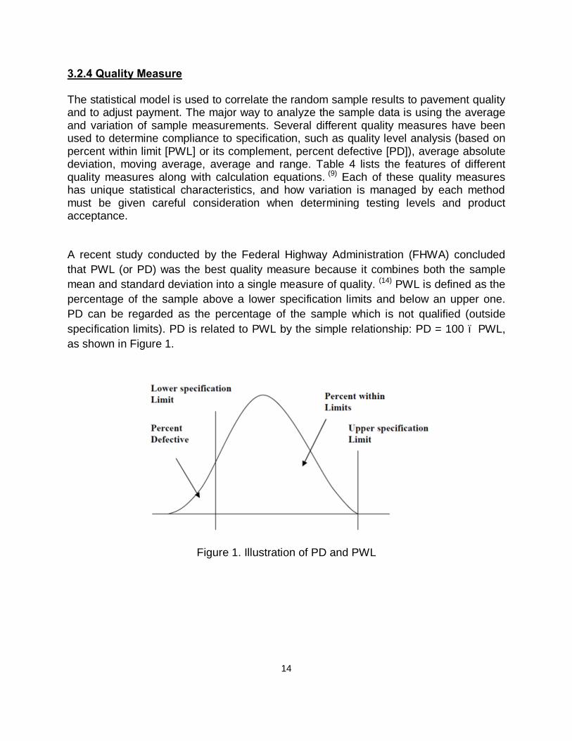
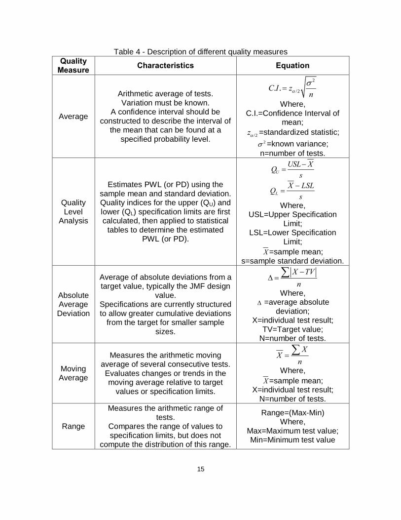
3.2.4 Quality Measure The statistical model is used to correlate the random sample results to pavement quality and to adjust payment. The major way to analyze the sample data is using the average and variation of sample measurements. Several different quality measures have been used to determine compliance to specification, such as quality level analysis (based on percent within limit [PWL] or its complement, percent defective [PD]), average absolute deviation, moving average, average and range. Table 4 lists the features of different quality measures along with calculation equations. (9) Each of these quality measures has unique statistical characteristics, and how variation is managed by each method must be given careful consideration when determining testing levels and product acceptance. A recent study conducted by the Federal Highway Administration (FHWA) concluded that PWL (or PD) was the best quality measure because it combines both the sample mean and standard deviation into a single measure of quality. (14) PWL is defined as the percentage of the sample above a lower specification limits and below an upper one. PD can be regarded as the percentage of the sample which is not qualified (outside specification limits). PD is related to PWL by the simple relationship: PD = 100 – PWL, as shown in Figure 1.

Figure 1. Illustration of PD and PWL

15

Table 4 - Description of different quality measures Quality

Measure Characteristics Equation

Average

Arithmetic average of tests. Variation must be known.

A confidence interval should be constructed to describe the interval of

the mean that can be found at a specified probability level.

2

/2. .C I znα

σ=

Where, C.I.=Confidence Interval of

mean; /2zα =standardized statistic;

2σ =known variance; n=number of tests.

Quality Level

Analysis

Estimates PWL (or PD) using the sample mean and standard deviation. Quality indices for the upper (QU) and lower (QL) specification limits are first calculated, then applied to statistical

tables to determine the estimated PWL (or PD).

UUSL XQ

s−

=

LX LSLQ

s−

=

Where, USL=Upper Specification

Limit; LSL=Lower Specification

Limit; X =sample mean;

s=sample standard deviation.

Absolute Average Deviation

Average of absolute deviations from a target value, typically the JMF design

value. Specifications are currently structured to allow greater cumulative deviations

from the target for smaller sample sizes.

X TVn−

∆ = ∑

Where, ∆ =average absolute

deviation; X=individual test result;

TV=Target value; N=number of tests.

Moving Average

Measures the arithmetic moving average of several consecutive tests. Evaluates changes or trends in the moving average relative to target

values or specification limits.

XX

n= ∑

Where, X =sample mean;

X=individual test result; N=number of tests.

Range

Measures the arithmetic range of tests.

Compares the range of values to specification limits, but does not

compute the distribution of this range.

Range=(Max-Min) Where,

Max=Maximum test value; Min=Minimum test value

16

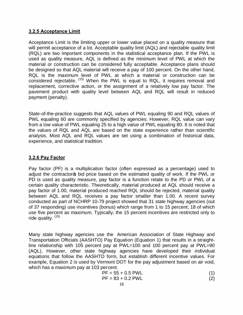
3.2.5 Acceptance Limit Acceptance Limit is the limiting upper or lower value placed on a quality measure that will permit acceptance of a lot. Acceptable quality limit (AQL) and rejectable quality limit (RQL) are two important components in the statistical acceptance plan. If the PWL is used as quality measure, AQL is defined as the minimum level of PWL at which the material or construction can be considered fully acceptable. Acceptance plans should be designed so that AQL material will receive a pay of 100 percent. On the other hand, RQL is the maximum level of PWL at which a material or construction can be considered rejectable. (15) When the PWL is equal to RQL, it requires removal and replacement, corrective action, or the assignment of a relatively low pay factor. The pavement product with quality level between AQL and RQL will result in reduced payment (penalty).

State-of-the-practice suggests that AQL values of PWL equaling 90 and RQL values of PWL equaling 60 are commonly specified by agencies. However, RQL value can vary from a low value of PWL equaling 25 to a high value of PWL equaling 80. It is noted that the values of RQL and AQL are based on the state experience rather than scientific analysis. Most AQL and RQL values are set using a combination of historical data, experience, and statistical tradition. 3.2.6 Pay Factor Pay factor (PF) is a multiplication factor (often expressed as a percentage) used to adjust the contractor’s bid price based on the estimated quality of work. If the PWL or PD is used as quality measure, pay factor is a function relate to the PD or PWL of a certain quality characteristic. Theoretically, material produced at AQL should receive a pay factor of 1.00, material produced reached RQL should be rejected, material quality between AQL and RQL receives a pay factor smaller than 1.00. A recent survey conducted as part of NCHRP 10-79 project showed that 31 state highway agencies (out of 37 responding) use incentives (bonus) which range from 1 to 15 percent; 18 of which use five percent as maximum. Typically, the 15 percent incentives are restricted only to ride quality. (15)

Many state highway agencies use the American Association of State Highway and Transportation Officials (AASHTO) Pay Equation (Equation 1) that results in a straight-line relationship with 105 percent pay at PWL=100 and 100 percent pay at PWL=90 (AQL). However, other state highway agencies have developed their individual equations that follow the AASHTO form, but establish different incentive values. For example, Equation 2 is used by Vermont DOT for the pay adjustment based on air void, which has a maximum pay at 103 percent.

PF = 55 + 0.5 PWL (1) PF = 83 + 0.2 PWL (2)

17

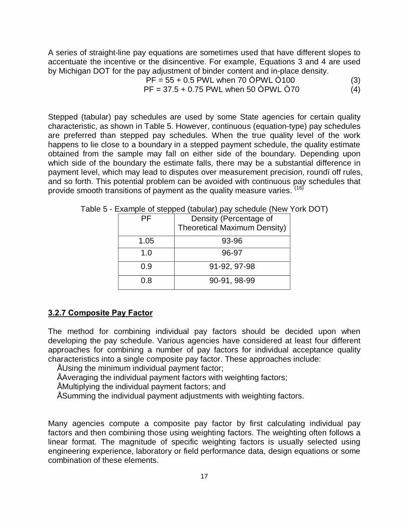
A series of straight-line pay equations are sometimes used that have different slopes to accentuate the incentive or the disincentive. For example, Equations 3 and 4 are used by Michigan DOT for the pay adjustment of binder content and in-place density.

PF = 55 + 0.5 PWL when 70 ≤ PWL ≤ 100 (3) PF = 37.5 + 0.75 PWL when 50 ≤ PWL ≤ 70 (4)

Stepped (tabular) pay schedules are used by some State agencies for certain quality characteristic, as shown in Table 5. However, continuous (equation-type) pay schedules are preferred than stepped pay schedules. When the true quality level of the work happens to lie close to a boundary in a stepped payment schedule, the quality estimate obtained from the sample may fall on either side of the boundary. Depending upon which side of the boundary the estimate falls, there may be a substantial difference in payment level, which may lead to disputes over measurement precision, round–off rules, and so forth. This potential problem can be avoided with continuous pay schedules that provide smooth transitions of payment as the quality measure varies. (16)

Table 5 - Example of stepped (tabular) pay schedule (New York DOT) PF Density (Percentage of

Theoretical Maximum Density) 1.05 93-96 1.0 96-97

0.9 91-92, 97-98

0.8 90-91, 98-99

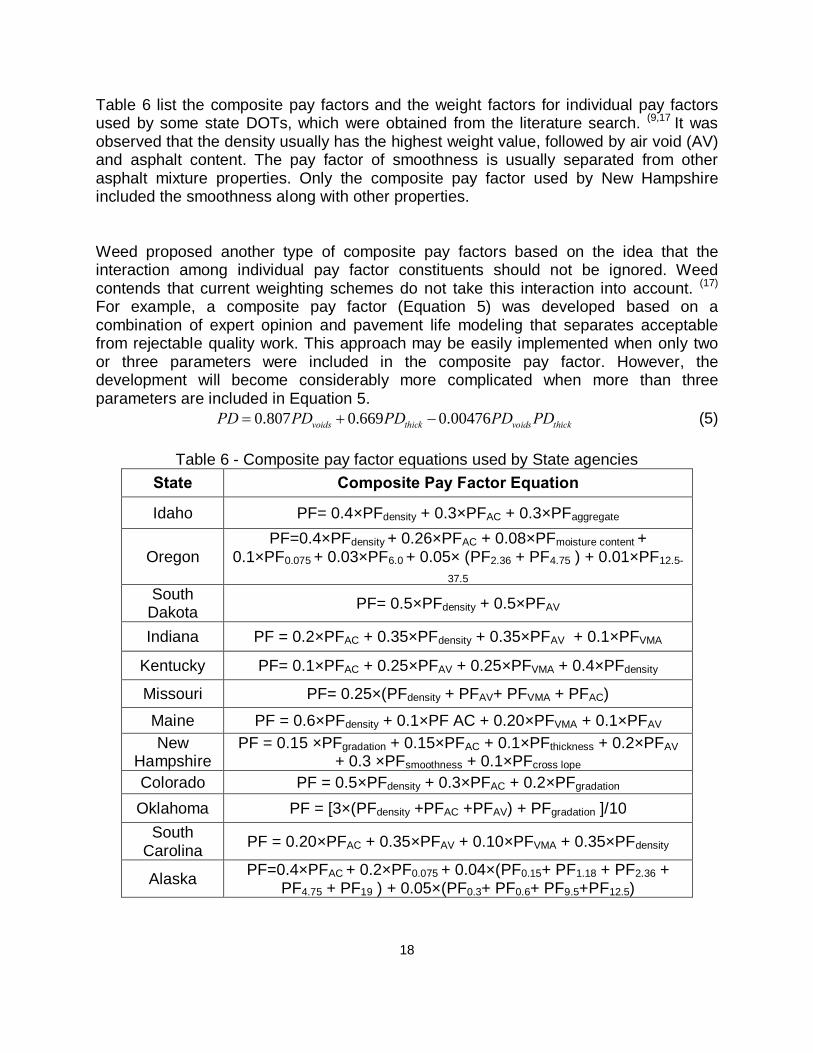
3.2.7 Composite Pay Factor The method for combining individual pay factors should be decided upon when developing the pay schedule. Various agencies have considered at least four different approaches for combining a number of pay factors for individual acceptance quality characteristics into a single composite pay factor. These approaches include: • Using the minimum individual payment factor; • Averaging the individual payment factors with weighting factors; • Multiplying the individual payment factors; and • Summing the individual payment adjustments with weighting factors. Many agencies compute a composite pay factor by first calculating individual pay factors and then combining those using weighting factors. The weighting often follows a linear format. The magnitude of specific weighting factors is usually selected using engineering experience, laboratory or field performance data, design equations or some combination of these elements.

18

Table 6 list the composite pay factors and the weight factors for individual pay factors used by some state DOTs, which were obtained from the literature search. (9,17 It was observed that the density usually has the highest weight value, followed by air void (AV) and asphalt content. The pay factor of smoothness is usually separated from other asphalt mixture properties. Only the composite pay factor used by New Hampshire included the smoothness along with other properties. Weed proposed another type of composite pay factors based on the idea that the interaction among individual pay factor constituents should not be ignored. Weed contends that current weighting schemes do not take this interaction into account. (17) For example, a composite pay factor (Equation 5) was developed based on a combination of expert opinion and pavement life modeling that separates acceptable from rejectable quality work. This approach may be easily implemented when only two or three parameters were included in the composite pay factor. However, the development will become considerably more complicated when more than three parameters are included in Equation 5.

0.807 0.669 0.00476voids thick voids thickPD PD PD PD PD= + − (5)

Table 6 - Composite pay factor equations used by State agencies State Composite Pay Factor Equation

Idaho PF= 0.4×PFdensity + 0.3×PFAC + 0.3×PFaggregate

Oregon PF=0.4×PFdensity + 0.26×PFAC + 0.08×PFmoisture content +

0.1×PF0.075 + 0.03×PF6.0 + 0.05× (PF2.36 + PF4.75 ) + 0.01×PF12.5-

37.5 South

Dakota PF= 0.5×PFdensity + 0.5×PFAV

Indiana PF = 0.2×PFAC + 0.35×PFdensity + 0.35×PFAV + 0.1×PFVMA

Kentucky PF= 0.1×PFAC + 0.25×PFAV + 0.25×PFVMA + 0.4×PFdensity

Missouri PF= 0.25×(PFdensity + PFAV+ PFVMA + PFAC)

Maine PF = 0.6×PFdensity + 0.1×PF AC + 0.20×PFVMA + 0.1×PFAV New

Hampshire PF = 0.15 ×PFgradation + 0.15×PFAC + 0.1×PFthickness + 0.2×PFAV

+ 0.3 ×PFsmoothness + 0.1×PFcross lope Colorado PF = 0.5×PFdensity + 0.3×PFAC + 0.2×PFgradation Oklahoma PF = [3×(PFdensity +PFAC +PFAV) + PFgradation ]/10

South Carolina PF = 0.20×PFAC + 0.35×PFAV + 0.10×PFVMA + 0.35×PFdensity

Alaska PF=0.4×PFAC + 0.2×PF0.075 + 0.04×(PF0.15+ PF1.18 + PF2.36 + PF4.75 + PF19 ) + 0.05×(PF0.3+ PF0.6+ PF9.5+PF12.5)

19

3.2.8 Risk Samples may not accurately reflect the quality of the construction. Concept of risk is introduced to adjust the error cause by the samples. There are two types of risk:

(1) Acceptable construction quality will be rejected (contractor’ risk). (2) Unacceptable construction quality will be accepted (agency’s risk).

The first type of risk is the contractor’s risk. It can also be expressed as material produced at AQL will be rejected or result in reduced payment. It will cause the unnecessary material removal and reconstruction. The second type of risk is the agency’s risk. It can be explained as material produced at RQL will be accepted or be accepted with bonus. It will result in poor pavement performance and unnecessary maintenance expenses. Typically, increasing sample size will reduce the risk. To reduce the inspection cost, the agency always seeks to achieve an optimal balance in sample size and inspection costs. To measure the risks involved in a particular acceptance plan, an operating characteristic (OC) curve that describes the relationship between a lot’s quality and its probability of acceptance for a given sample size is needed. A computer simulation program called OCPLOT, developed in FHWA Demonstration Project 89 by Weed, is available for the generation of OC curves. (18) The factors considered in OCPLOT include sample sizes, pay factor equation, specification limits, and retest provisions. The program allows the user to assess both the contractor’s risk ant the agency’s risk). Recently, a new computer program, SPECRISK, has been developed that is capable of analyzing these risks under a wide variety of conditions that typically occur in highway applications. (19) The new SPECRISK can analyze specifications based on either PWL (percent within limits) or PD (percent defective) as the statistical quality measure, and can handle up to five separate quality characteristics simultaneously, any or all of which may be correlated to any specified degree. 3.3 HMA Quality Characteristics and Test Methods

Typical HMA Quality characteristics that are evaluated in the QA/QC Specification include air voids (or density) of the compacted mix either in the laboratory or in the field, asphalt binder content, and aggregate gradation. Other properties such as layer thickness, segregation, volumetric properties of asphalt mixture also have certain influences in pavement performance. Before the development of the performance-related specification and pay adjustment, the following factors should be considered:

1) Identify material- and construction-related HMA properties that are determined to be significant predictors of pavement performance and over which the contractor has control;

2) Establish reliable test procedures for measuring the identified HMA properties based on laboratory testing of compacted mixtures and/or field cores.

20

3.3.1 Material and Construction Variables Affecting Pavement Performance

A literature search was conducted to identify the material- and construction-related properties that are significant predictors of pavement performance and are under the contractor’s control. The results indicate that most of the studies conducted to date have focused on evaluating compositional, volumetric, and fundamental engineering properties of HMA specimens or field cores through laboratory testing. In-Place Air Void Content (In-Place Density) In-pace air void (or density) is an important factor as an asphalt pavement quality indicator, which is dependent on the asphalt content, aggregate gradation, and nominal maximum aggregate sizes (NMAS). Overall, air void has a direct impact on density, rutting, fatigue life, permeability, oxidation, bleeding and so on. The in-place air void content (or density) has been found as the most influential property affecting the performance and durability of an HMA pavement by previous studies. In most of DOT construction specifications, in-place density is measured as a percent of maximum theoretical density with ranges between 91 and 98 percent (mostly between 92 and 97 percent) to control the air void contents of the constructed pavements. (20)

The optimum air void content is important to the pavement performance. A compacted mixture with low air voids can result in rutting (shear flow), shoving, and bleeding. Ford claimed that HMA mixtures must be constructed to maintain air voids content above a minimum level (2.5 percent) to avoid hydroplaning caused by development of rut depth. (21) Brown and Cross found that in-place air void contents below three percent will greatly increase the probability of premature rutting. (22) On the other hand, pavements constructed with high air voids can increase the potential for moisture damage, oxidation, raveling, and cracking. Meanwhile, high air voids can contribute to the development of rutting in the wheel paths due to consolidation caused by traffic loading. Early research has suggested that for each one percent increase in air voids (compared to seven percent air void content) there is a 10 percent loss of pavement life (approximately one year). (23) Santucci et al. concluded that the mixtures should maintain the air void contents lower than eight percent to avoid rapid oxidation and subsequent cracking or raveling. (24) Flintsch et al. have found that excess air voids will lead to lower resilient modulus and lower dynamic modulus of asphalt mixtures. (25) Similarly, Vivar and Haddock found that HMA mixtures with lower density always have higher permeability, lower dynamic modulus, lower flexural stiffness, and shorter fatigue life. (26) Asphalt Content Asphalt content is another major indicator to reflect pavement performance. Similar to air void content, asphalt binder content affects HMA mixture performance in stiffness, strength, durability, fatigue life, raveling, rutting, and moisture damage. The binder

21

content to be added to asphalt mixture cannot be too excessive or too little. The optimum amount of binder content should include sufficient amount of binder to fully coat the aggregates with bitumen and seal up the voids within the mixture without causing bleeding. Tran and Hall concluded that increased asphalt content resulted in increased thickness of the binder film between aggregate particles, which increased the proportion of asphalt over a cross-section. (27) Since the load-induced tensile strains are mainly concentrated in the asphalt binder, thicker films means smaller binder strain. Therefore, increased asphalt content may result in an increase in laboratory fatigue life and a decrease in mixture stiffness. Harvey and Tsai conducted a strain-controlled flexural beam testing and found the similar result. (28) They quantified that in relatively thicker pavements, fatigue life can increase approximately 10 percent for each 0.5 percent increase in asphalt content. This effect is more significant in the thin pavement structure: approximately 20 percent increase in fatigue life for each 0.5 percent increase in asphalt content. Mauplin and Diefenderfer claimed that high-binder mixes would possibly be less susceptible to moisture damage because of the less chance for water to penetrate the thick asphalt film. (29) Therefore, increasing the binder content of asphalt mixture beyond the design optimum could greatly decrease the fatigue cracking potential. However, excessive binder content will weaken the resistance to deformation of asphalt pavement under traffic load. Flintsch et al. concluded that higher asphalt content resulted in lower resilient modulus and dynamic modulus to all frequencies that increased rutting potential of asphalt pavement. (25) Aggregate Gradation The overall stability of HMA largely depends on aggregate properties. Mixes with different aggregate gradations are likely to present different rutting potential. Coarse-graded mixes contain a relatively higher percentage of coarse aggregate than fine-graded mixes and will lead to larger voids, which make the mix more permeable. To fill these voids, coarse graded mixes may require more asphalt content. Kandhal and Mallick found that the effect of gradation on granite and limestone wearing and binder courses is significant (PG 64-22 asphalt was used). (30) Gradation below restricted zone shows higher rutting compared to above and through restricted zone. Vivar and Haddoc concluded that coarse-graded mixtures tend to have lower dynamic modulus, flexural stiffness and fatigue life compared to fine-graded mixtures. (26) They also compared the mixtures with a 19.0-mm NMAS to the mixtures with a 9.5-mm NMAS. Results show that mixtures with a 19.0-mm NMAS usually have higher dynamic modulus and flexural stiffness, higher permeability and moisture damage, and lower fatigue life than those with a 9.5-mm nominal maximum aggregate size (NMAS).

22

Permeability Permeability is the ability of a material (in this case HMA) to transmit fluids (in this case water) through its pores when subjected to pressure, or a difference in water head. With the implementation of Superpave mix design, HMA gradations are coarser than in previous years, which results in relatively high permeability of pavements. Pavements with high permeability will rapidly deteriorate (stripping and oxidation) due to water and air infiltration. Therefore, measurement of permeability along with density will give a better indication of a pavement’s durability than measurement of density alone. Brown et al. found that for a given air void level, coarse-graded mixtures typically have higher permeability values than the fine-graded mixtures. (20) According to Mallick et al., for a given in-place air void content, the permeability of HMA can increase by one order of magnitude as the increasing of maximum aggregate size. (31) Vivar and Haddock developed an exponential relationship between in-situ air void and permeability and showed that when air void content was greater than eight percent, permeability increases exponentially. (26) Cooley et al. has shown that the lift thickness and Nominal Maximum Aggregate Size (NMAS) can significantly affect the relationship between density and permeability. (32) Segregation Segregation refers to the non-uniform distribution of coarse and fine aggregates. Segregated mixtures generally do not conform to the original job mix formula and, as a result, such areas may exhibit poor structural and textural characteristics, which in turn result in poor performance. Segregation is more prevalent in coarser mixtures and especially gap-graded mixtures. The reduction of asphalt content may reduce the cohesion, which also can lead to segregation. (33) A study conducted by Williams et al. indicates that the coarsely segregated asphalt mixture is associated with low asphalt content and has a shorter fatigue life. (34) The finely segregated mixture exhibited a longer fatigue life; however, the lack of sufficient coarse aggregates in combination with the high asphalt content would make the mix more susceptible to rutting. Pavement Thickness Asphalt pavement is designed to have enough thickness to reduce the tensile strains at the bottom of asphalt layer and resist bottom-up fatigue cracking. Non-uniform layer thickness may affect the surface profile and may result in insufficient layer thickness, as a result of which the pavement structure may not be structurally capable to carry the traffic loads. The ride quality can be also affected by the non-uniformity in the layer thickness. Chatti et al. stated that pavements with HMA surface layer thickness approximately four inches show more fatigue cracking, slightly more rutting, and higher changes in IRI than those with surface layer with seven inches. (35)

23

Prowell reported that as-built asphalt lift thicknesses ranging from 9.7 to 11.2 cm were for an as-designed thickness of 10.2 cm in the test track in the National Center for Asphalt Technology (NCAT). (36) Freeman and Grogan performed a thorough review and reported the properties of multiple pavement materials.8 Coefficients of variation reported were 10 and 15 percent for asphalt layer and granular base layer thickness, respectively. 3.3.2 Test Methods for Measuring HMA Quality Characteristics

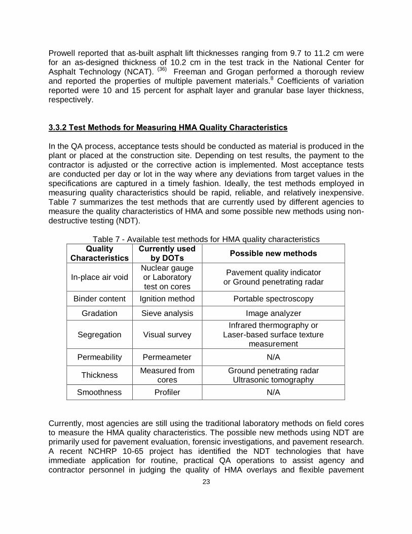
In the QA process, acceptance tests should be conducted as material is produced in the plant or placed at the construction site. Depending on test results, the payment to the contractor is adjusted or the corrective action is implemented. Most acceptance tests are conducted per day or lot in the way where any deviations from target values in the specifications are captured in a timely fashion. Ideally, the test methods employed in measuring quality characteristics should be rapid, reliable, and relatively inexpensive. Table 7 summarizes the test methods that are currently used by different agencies to measure the quality characteristics of HMA and some possible new methods using non-destructive testing (NDT).

Table 7 - Available test methods for HMA quality characteristics Quality

Characteristics Currently used

by DOTs Possible new methods

In-place air void Nuclear gauge or Laboratory test on cores

Pavement quality indicator or Ground penetrating radar

Binder content Ignition method Portable spectroscopy

Gradation Sieve analysis Image analyzer

Segregation Visual survey Infrared thermography or

Laser-based surface texture measurement

Permeability Permeameter N/A

Thickness Measured from cores

Ground penetrating radar Ultrasonic tomography

Smoothness Profiler N/A Currently, most agencies are still using the traditional laboratory methods on field cores to measure the HMA quality characteristics. The possible new methods using NDT are primarily used for pavement evaluation, forensic investigations, and pavement research. A recent NCHRP 10-65 project has identified the NDT technologies that have immediate application for routine, practical QA operations to assist agency and contractor personnel in judging the quality of HMA overlays and flexible pavement

24

construction. (37) However, further studies are needed to investigate the application of the NDT devices through pilot field and laboratory tests before its real implementation for QA purposes. 3.4 Performance-Related Pay Adjustment

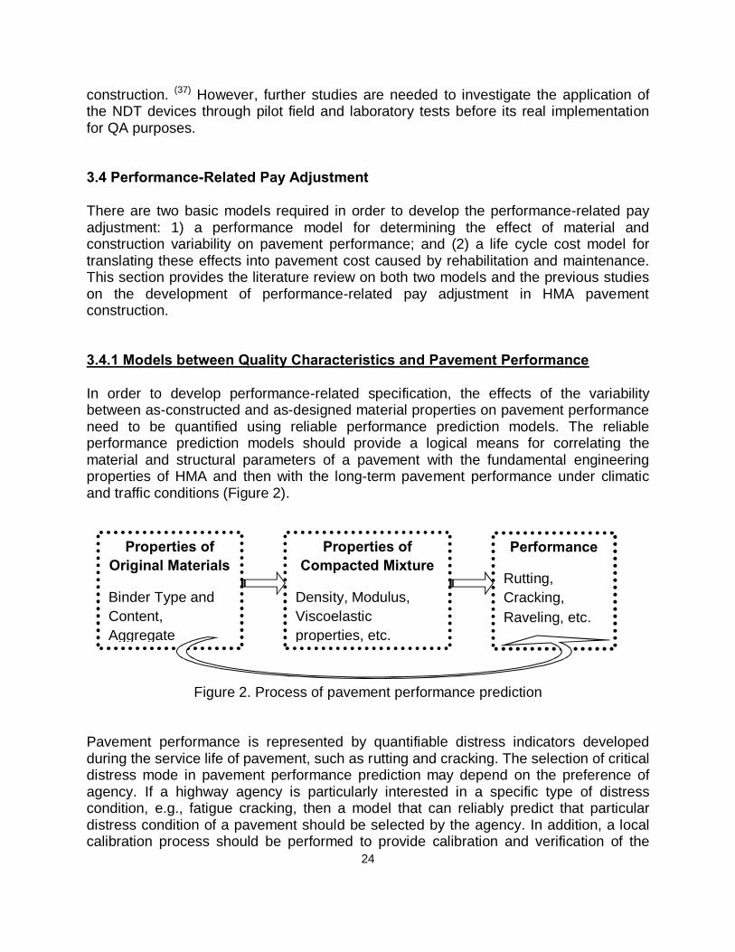
There are two basic models required in order to develop the performance-related pay adjustment: 1) a performance model for determining the effect of material and construction variability on pavement performance; and (2) a life cycle cost model for translating these effects into pavement cost caused by rehabilitation and maintenance. This section provides the literature review on both two models and the previous studies on the development of performance-related pay adjustment in HMA pavement construction. 3.4.1 Models between Quality Characteristics and Pavement Performance In order to develop performance-related specification, the effects of the variability between as-constructed and as-designed material properties on pavement performance need to be quantified using reliable performance prediction models. The reliable performance prediction models should provide a logical means for correlating the material and structural parameters of a pavement with the fundamental engineering properties of HMA and then with the long-term pavement performance under climatic and traffic conditions (Figure 2).

Figure 2. Process of pavement performance prediction Pavement performance is represented by quantifiable distress indicators developed during the service life of pavement, such as rutting and cracking. The selection of critical distress mode in pavement performance prediction may depend on the preference of agency. If a highway agency is particularly interested in a specific type of distress condition, e.g., fatigue cracking, then a model that can reliably predict that particular distress condition of a pavement should be selected by the agency. In addition, a local calibration process should be performed to provide calibration and verification of the

Properties of Original Materials

Binder Type and Content, Aggregate

Properties of Compacted Mixture

Density, Modulus, Viscoelastic properties, etc.

Performance

Rutting, Cracking, Raveling, etc.

25

predictive models so that they may accurately predict pavement conditions in the specific region. The literature review has shown that although many performance models have been developed over the past decade for specific distress modes, the recently developed Mechanistic-Empirical Pavement Design Guide (MEPDG) provides the best state-of-art approach to predict pavement performance considering the interaction between traffic, material, environment and structure. The MEPDG contains models for predicting HMA permanent deformation, fatigue cracking (bottom-up and top-down), and thermal cracking. Smoothness is then calculated based on the distresses predicted as well as the original, initial as-built smoothness level after construction. Three levels of input are available in the MEPDG procedure to predict pavement performance, including a number of volumetric and mechanistic properties of HMA. For example, Level 1 input parameters consist of measured mechanistic HMA properties such as the dynamic modulus. Level 2 input parameters include asphalt cement content, binder viscosity, aggregate gradation, and air void content. These inputs are used to predict the fundamental properties used in the Level 1 analysis. Therefore, variability in volumetric and mechanistic design inputs can be considered in the prediction of pavement performance using the MEPDG procedure. Several studies have been conducted to analyze the sensitivity of MEPDG output subject to different material and structure alternatives, but few studies evaluated the sensitivity of pavement performance prediction subject to the variability in the design inputs related to material and construction. Kim et al. investigated the relative sensitivity of MEPDG input parameters related to the properties of ACC, traffic, and climate in two existing Iowa flexible pavement structures. (38) It was found that the sensitivity of prediction varies depending on performance indicator and pavement structure, for example, the predicted longitudinal cracking performance measure was influenced by most input parameters, while IRI was not sensitive for most input parameters. Aguiar-Moya and Prozzi evaluated the effects of field variability of design inputs on the performance predicted using the MEPDG software. (39) Two pavement structures (thin HMA and thick HMA) in three climate regions (cool, warm, and hot) were evaluated. Results showed that several design variables cause considerable variation in the predicted performance even when the average coefficients of variation were not large (under 10 percent). It is noted that in the process of pavement performance prediction, of greater importance is statistics’ role in determining the level of reliability in predicted pavement performance. In other words, it is obvious that there is a level of confidence associated with the prediction of distresses when the variations in the material- and construction-related parameters are considered. Statistics is needed to determine this level of

26

confidence and, accordingly, to assist in making decisions on the acceptability of a certain design or construction. A number of simulation techniques have been developed to establish the distribution of the response variable according to the probabilistic characteristics of the input random variable. Therefore, the techniques that can accurately account for the uncertainty of input variables in pavement reliability analysis will be explored in development of pay adjustment during this study. 3.4.2 Development of Performance-Related Pay Factor Early Studies Anderson et al. proposed a preliminary framework for PRSs for asphalt concrete pavements. (40) Target material- and construction-related variables include thickness, compaction, roughness, asphalt content, gradation and others. The design algorithms are used to determine the predicted life cycle cost (LCC) for the target and as-built pavement. Acceptance plan and payment schedule are then adjusted according to the result. The pay adjustment considers the maintenance, rehabilitation, and user costs. The pay factor (PF) is calculated in Equation 6.

PF=100(LBP-C)/LBP (6) Where, LBP =lot bid price; C = (Ac-At){[(1+i)Lc-1]/[i(1+i)Lt}; Ac = annualized total cost at economic life of as-constructed pavement; At = annualized total cost at economic life of target pavement; Lc = economic life of as-constructed pavement; and Lt = economic life of target pavement. Shook et al. used the AASHTO Guide equations which estimate pavement service life as the number of equivalent single axle loads (ESALs) to failure. Material- and construction-related variables include asphalt content, percent passing the #30 sieve and the #200 sieve, VMA, and air voids. The pay factor methods related to LCC is shown in Equation 7. (41)

PF=100[1+C0 (RLd-RLe)/Cp (1-RLo)] (7) Where, Cp = percent unit cost of pavement, Co = percent unit cost of overlay, Ld = design life of pavement, Le = expected life of pavement, Lo = expected life of overlay, R = (1 + Rinf / 100) / (1 + Rint / 100), Rinf = annual inflation rate, and Rint= annual interest rate. Solaimanian et al. developed a prototype PRS based on VESYS. (42) VESYS was the

27

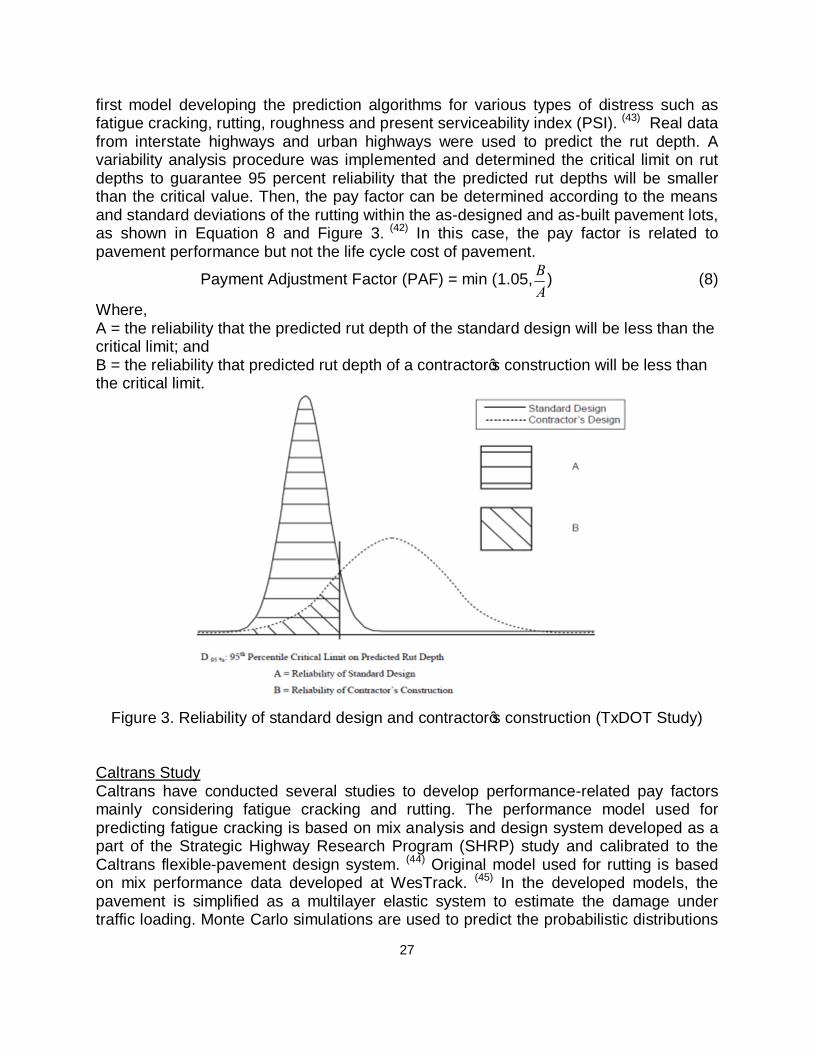
first model developing the prediction algorithms for various types of distress such as fatigue cracking, rutting, roughness and present serviceability index (PSI). (43) Real data from interstate highways and urban highways were used to predict the rut depth. A variability analysis procedure was implemented and determined the critical limit on rut depths to guarantee 95 percent reliability that the predicted rut depths will be smaller than the critical value. Then, the pay factor can be determined according to the means and standard deviations of the rutting within the as-designed and as-built pavement lots, as shown in Equation 8 and Figure 3. (42) In this case, the pay factor is related to pavement performance but not the life cycle cost of pavement.

Payment Adjustment Factor (PAF) = min (1.05, BA

) (8)

Where, A = the reliability that the predicted rut depth of the standard design will be less than the critical limit; and B = the reliability that predicted rut depth of a contractor’s construction will be less than the critical limit.

Figure 3. Reliability of standard design and contractor’s construction (TxDOT Study)

Caltrans Study Caltrans have conducted several studies to develop performance-related pay factors mainly considering fatigue cracking and rutting. The performance model used for predicting fatigue cracking is based on mix analysis and design system developed as a part of the Strategic Highway Research Program (SHRP) study and calibrated to the Caltrans flexible-pavement design system. (44) Original model used for rutting is based on mix performance data developed at WesTrack. (45) In the developed models, the pavement is simplified as a multilayer elastic system to estimate the damage under traffic loading. Monte Carlo simulations are used to predict the probabilistic distributions

28

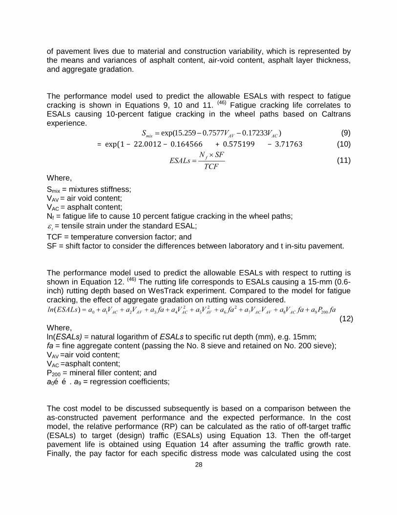
of pavement lives due to material and construction variability, which is represented by the means and variances of asphalt content, air-void content, asphalt layer thickness, and aggregate gradation. The performance model used to predict the allowable ESALs with respect to fatigue cracking is shown in Equations 9, 10 and 11. (46) Fatigue cracking life correlates to ESALs causing 10-percent fatigue cracking in the wheel paths based on Caltrans experience.

exp(15.259 0.7577 0.17233 )mix AV ACS V V= − − (9) �� = exp(1 − 22.0012 − 0.164566�� + 0.575199�� − 3.71763�� (10)

fN SFESALs

TCF×

=

(11)

Where, Smix = mixtures stiffness;

VAV = air void content; VAC = asphalt content; Nf = fatigue life to cause 10 percent fatigue cracking in the wheel paths;

tε = tensile strain under the standard ESAL; TCF = temperature conversion factor; and SF = shift factor to consider the differences between laboratory and t in-situ pavement. The performance model used to predict the allowable ESALs with respect to rutting is shown in Equation 12. (46) The rutting life corresponds to ESALs causing a 15-mm (0.6-inch) rutting depth based on WesTrack experiment. Compared to the model for fatigue cracking, the effect of aggregate gradation on rutting was considered.

2 2 20 1 2 3 4 5 6 7 8 9 200( ) AC AV AC AV AC AV ACln ESALs a a V a V a fa a V a V a fa a V V a V fa a P fa= + + + + + + + + +

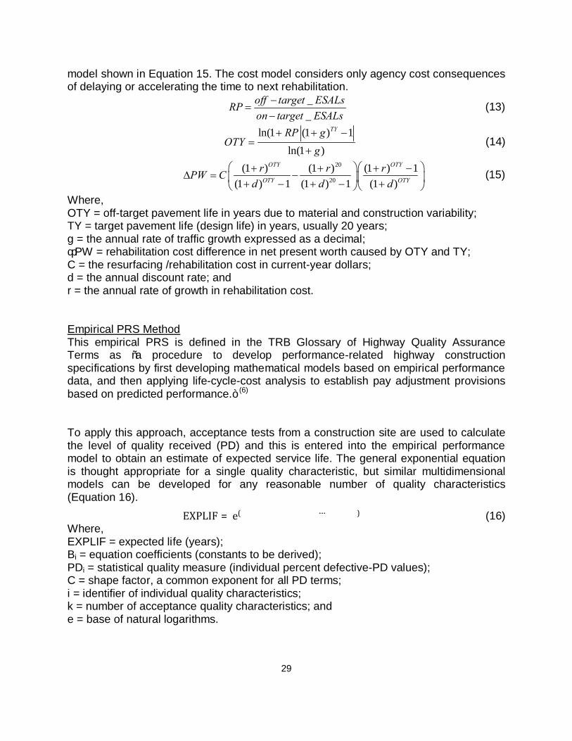
(12) Where, ln(ESALs) = natural logarithm of ESALs to specific rut depth (mm), e.g. 15mm; fa = fine aggregate content (passing the No. 8 sieve and retained on No. 200 sieve); VAV =air void content; VAC =asphalt content; P200 = mineral filler content; and a0……. a9 = regression coefficients; The cost model to be discussed subsequently is based on a comparison between the as-constructed pavement performance and the expected performance. In the cost model, the relative performance (RP) can be calculated as the ratio of off-target traffic (ESALs) to target (design) traffic (ESALs) using Equation 13. Then the off-target pavement life is obtained using Equation 14 after assuming the traffic growth rate. Finally, the pay factor for each specific distress mode was calculated using the cost

29

model shown in Equation 15. The cost model considers only agency cost consequences of delaying or accelerating the time to next rehabilitation.

__

off target ESALsRPon target ESALs

−=

− (13)

ln(1 (1 ) 1

ln(1 )

TYRP gOTY

g+ + −

=+

(14)

20

20

(1 ) (1 ) (1 ) 1(1 ) 1 (1 ) 1 (1 )

OTY OTY

OTY OTY

r r rPW Cd d d

+ + + −∆ = − + − + − +

(15)

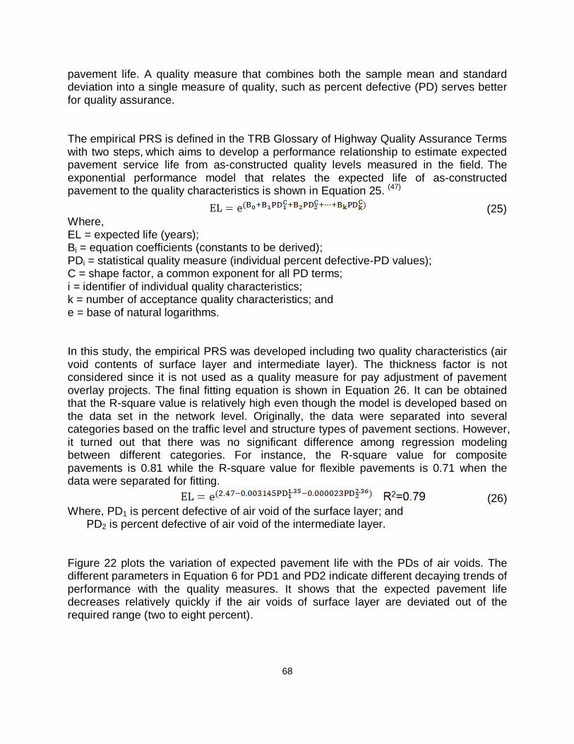
Where, OTY = off-target pavement life in years due to material and construction variability; TY = target pavement life (design life) in years, usually 20 years; g = the annual rate of traffic growth expressed as a decimal; ΔPW = rehabilitation cost difference in net present worth caused by OTY and TY; C = the resurfacing /rehabilitation cost in current-year dollars; d = the annual discount rate; and r = the annual rate of growth in rehabilitation cost. Empirical PRS Method This empirical PRS is defined in the TRB Glossary of Highway Quality Assurance Terms as “a procedure to develop performance-related highway construction specifications by first developing mathematical models based on empirical performance data, and then applying life-cycle-cost analysis to establish pay adjustment provisions based on predicted performance.” (6) To apply this approach, acceptance tests from a construction site are used to calculate the level of quality received (PD) and this is entered into the empirical performance model to obtain an estimate of expected service life. The general exponential equation is thought appropriate for a single quality characteristic, but similar multidimensional models can be developed for any reasonable number of quality characteristics (Equation 16).

EXPLIF = e(��

��···��) (16)

Where, EXPLIF = expected life (years); Bi = equation coefficients (constants to be derived); PDi = statistical quality measure (individual percent defective-PD values); C = shape factor, a common exponent for all PD terms; i = identifier of individual quality characteristics; k = number of acceptance quality characteristics; and e = base of natural logarithms.

30

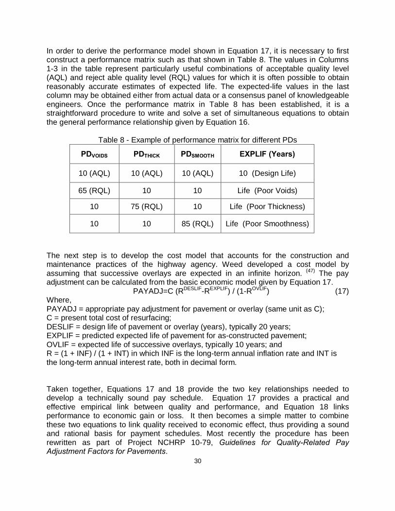
In order to derive the performance model shown in Equation 17, it is necessary to first construct a performance matrix such as that shown in Table 8. The values in Columns 1-3 in the table represent particularly useful combinations of acceptable quality level (AQL) and reject able quality level (RQL) values for which it is often possible to obtain reasonably accurate estimates of expected life. The expected-life values in the last column may be obtained either from actual data or a consensus panel of knowledgeable engineers. Once the performance matrix in Table 8 has been established, it is a straightforward procedure to write and solve a set of simultaneous equations to obtain the general performance relationship given by Equation 16.

Table 8 - Example of performance matrix for different PDs

PDVOIDS PDTHICK PDSMOOTH EXPLIF (Years)

10 (AQL) 10 (AQL) 10 (AQL) 10 (Design Life)

65 (RQL) 10 10 Life (Poor Voids)

10 75 (RQL) 10 Life (Poor Thickness)

10 10 85 (RQL) Life (Poor Smoothness)

The next step is to develop the cost model that accounts for the construction and maintenance practices of the highway agency. Weed developed a cost model by assuming that successive overlays are expected in an infinite horizon. (47) The pay adjustment can be calculated from the basic economic model given by Equation 17.

PAYADJ=C (RDESLIF-REXPLIF) / (1-ROVLIF) (17) Where, PAYADJ = appropriate pay adjustment for pavement or overlay (same unit as C); C = present total cost of resurfacing; DESLIF = design life of pavement or overlay (years), typically 20 years; EXPLIF = predicted expected life of pavement for as-constructed pavement; OVLIF = expected life of successive overlays, typically 10 years; and R = (1 + INF) / (1 + INT) in which INF is the long-term annual inflation rate and INT is the long-term annual interest rate, both in decimal form. Taken together, Equations 17 and 18 provide the two key relationships needed to develop a technically sound pay schedule. Equation 17 provides a practical and effective empirical link between quality and performance, and Equation 18 links performance to economic gain or loss. It then becomes a simple matter to combine these two equations to link quality received to economic effect, thus providing a sound and rational basis for payment schedules. Most recently the procedure has been rewritten as part of Project NCHRP 10-79, Guidelines for Quality-Related Pay Adjustment Factors for Pavements.

31

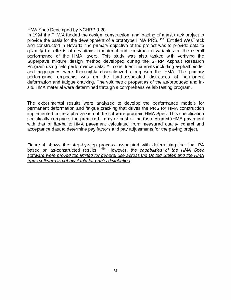
HMA Spec Developed by NCHRP 9-20 In 1994 the FHWA funded the design, construction, and loading of a test track project to provide the basis for the development of a prototype HMA PRS. (48) Entitled WesTrack and constructed in Nevada, the primary objective of the project was to provide data to quantify the effects of deviations in material and construction variables on the overall performance of the HMA layers. This study was also tasked with verifying the Superpave mixture design method developed during the SHRP Asphalt Research Program using field performance data. All constituent materials including asphalt binder and aggregates were thoroughly characterized along with the HMA. The primary performance emphasis was on the load-associated distresses of permanent deformation and fatigue cracking. The volumetric properties of the as-produced and in-situ HMA material were determined through a comprehensive lab testing program. The experimental results were analyzed to develop the performance models for permanent deformation and fatigue cracking that drives the PRS for HMA construction implemented in the alpha version of the software program HMA Spec. This specification statistically compares the predicted life-cycle cost of the “as-designed” HMA pavement with that of “as-built” HMA pavement calculated from measured quality control and acceptance data to determine pay factors and pay adjustments for the paving project. Figure 4 shows the step-by-step process associated with determining the final PA based on as-constructed results. (48) However, the capabilities of the HMA Spec software were proved too limited for general use across the United States and the HMA Spec software is not available for public distribution.

32

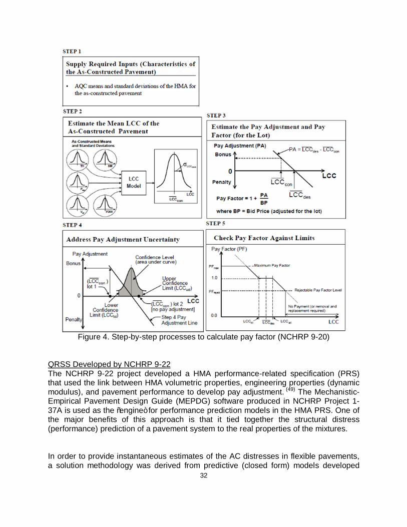
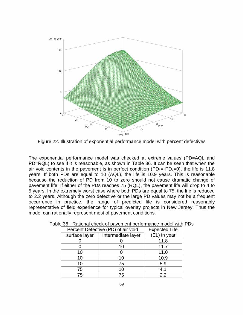
Figure 4. Step-by-step processes to calculate pay factor (NCHRP 9-20)

QRSS Developed by NCHRP 9-22 The NCHRP 9-22 project developed a HMA performance-related specification (PRS) that used the link between HMA volumetric properties, engineering properties (dynamic modulus), and pavement performance to develop pay adjustment. (49) The Mechanistic-Empirical Pavement Design Guide (MEPDG) software produced in NCHRP Project 1-37A is used as the “engine” for performance prediction models in the HMA PRS. One of the major benefits of this approach is that it tied together the structural distress (performance) prediction of a pavement system to the real properties of the mixtures. In order to provide instantaneous estimates of the AC distresses in flexible pavements, a solution methodology was derived from predictive (closed form) models developed

33

from a comprehensive set of factorial runs of the MEPDG software. As a result, a stand-alone program - Quality-Related Specification Software (QRSS) is developed. The QRSS calculates the predicted performance of an HMA pavement from the volumetric and materials properties of the as-designed HMA and compares it with that of the as-built pavement. The calculated differences for the permanent deformation, fatigue cracking, low-temperature cracking, and IRI determine pay factors for each lot or sub-lot. The predictions are probabilistic; they are calculated through a Monte Carlo procedure that uses historical standard deviations of the input properties in order to account for construction and testing variability. In the QRSS, pay factors (PF) are developed from predicted pavement life difference that is defined as the difference in predicted service life between the as-designed mix and the as-built mix, as shown in Figure 5. The Pay Factor Penalty/Bonus is estimated from the pavement life difference for each lot. The criterion relating the pavement life difference and pay factor for each distress is solely defined by the user agency. The summation of the pay factors for the lots provides the total project pay factor. It is noted that no life cycle cost is considered in the development of pay factor.

Figure 5. Illustration of predicted life difference and pay factors in QRSS (NCHRP 9-22) It should be noted that several simplified assumptions have been made in the development of QRSS in order to achieve the closed-form solutions for three major HMA distresses (rutting, fatigue cracking, and thermal cracking). These include:

• ESALs are used and no axle load spectrum approach for mixed traffic; • No seasonal changes for modulus of unbound materials; • Composite foundation modulus is used to represent all layers beneath the

HMA layers; • Cumulative annual temperature effects on HMA are accounted for by

“effective temperature concepts” which depends on distress type, environmental conditions at project site, vehicle speed, and thickness (depths) of each HMA layer.

34

3.5 Longitudinal Joint Density Specification 3.5.1 Longitudinal Joint Density Requirement There is a wide variation for how State agencies address joints in their specs. Recently, a growing number of agencies have implemented specifications for the longitudinal joint with the requirement on joint density. Although the construction method was not specified, agencies usually provide guidance to contractors in order to achieve better compaction quality at the longitudinal joint. A survey conducted by Asphalt Institute indicates that 35 states said they had some sort of longitudinal joint specification or special provision, but only 17 states reported that they had a minimum density requirement at the joint. (50) Among those 17 states with a minimum density requirement at the joint, the value ranged from 89 to 92 percent Theoretical Maximum Density (TMD).

Table 9 summarizes the mat and joint density specification used by a number of State agencies. (See references 51, 52, 53, and 54)

Table 9 - Mat and joint density specifications by different State agencies

State Measurement location

Mat density requirement Joint density requirement

Alaska Center of the joint 94%of TMD* 91% of TMD

Arizona Center of the joint

98% of lab density

The density required on the tapered joint is the same as

for the rest of the mat

Colorado Center of the joint

92-96% of TMD

92% of the max specific gravity, tolerance four

percent variation

Kansas 8 in. from the edge of mat 92% of TMD Interior Density - Joint

Density < 50 kg/m3

Kentucky Within 2.5-3.5

in. from the joint

89-96% of TMD 87-97% of TMD

Michigan Center of the joint 92% of TMD 89% of TMD

Nevada Hot side of joint

90-97% of TMD 90% of TMD

New York Center of the joint

92-97% of TMD0 90-97% of TMD

Texas Within 8 in. of the joint

90-97% of TMD

At least 90% of TMD and no more than 3%less than the

average mat density *TMD: Theoretical Maximum Density.

35

3.5.2 Pay Adjustment for Longitudinal Joint Density A quality joint density specification can be an effective way to improve pavement performance. Table 10 summarized the pay adjustment methods for the longitudinal joint density that have been identified from the literature review.

Table 10 - Literature review summary of pay adjustments for joint density

Agency Lot size Quality measure

Pay adjustment

Connecticut 2000 tons; four cores per lot Average density

Combined with mat density

Kentucky 4000 tons; two cores per 1000 tons

Average density


Pennsylvania 12,500 ft; one core per 2500 ft Percent within limit

Separately for joint

Alaska 5000 tons, one core at joint corresponding to mat coring

location

Average density


Vermont Total project length of joint constructed per pavement

course; two cores per joint mile

Percent of cores above

minimum density


Maine Total project length of joint constructed per pavement course; one core per 750 ft

Percent within limit


FAA The total length of longitudinal joints constructed by a lot of

mat material

Percent within limit


Army Corps of Engineers

2000 tons; four cores per 500 tons

Average density


The review shows that the pay adjustment on joint density is either based on the average value of joint density or the percent within limit calculated from the specification limits of the joint density. Only a few state DOTs and Federal agencies have established disincentive or even incentive pay adjustments for longitudinal joint density. This allows contractors to choose their own methods to deliver high density at the joint.

36

Connecticut DOT (55) Coring shall be performed on each lift specified to a thickness of one and one-half (1 ½) inches or more. For the density lot without bridge, the target lot size is 2000 tons and four cores are taken per lot. If the density lot has the total tonnage smaller than 500 tons, three cores will be taken per lift. The definition of density lots vary if the lot is on bridge or include bridge. Joint cores must be taken so that the center of the core is 5 inches from the visible joint on the hot mat side, Figure 6. The density of each core shall be determined using the production lot’s average maximum theoretical gravity established from the plant production testing. The production lot includes all material placed during a continuous daily paving operation.

Figure 6. Illustration of taking joint cores (After Connecticut DOT specification)

The quantity of bituminous concrete measured for payment for a specified lift of pavement 1½ inches or greater may be adjusted for density. Separate density adjustments will be made for each lot and will not be combined to establish one density adjustment. If either the mat or joint adjustment value is “remove and replace”, the density lot shall be removed and replaced (curb to curb). The pay equation is shown in Equation 18.

TD = [{(PAM x 0.50) + (PAJ x 0.50)} / 100] × Density Lot Tons (18) Where, TD = Total tons adjusted for density for each lot; PAM = Mat density percent adjustment; and PAJ = Joint density percent adjustment. Table 11 shows pay factors for mat and joint density used by Connecticut DOT. The density ranges for full payment and bonus is 92-98.5 percent of TMD for the mat density and 91-98.5 percent of TMD for the joint density, which has boundaries on both sides. When the joint density is below 87 percent of TMD, remove and replace is required.

Hot side Cold Side

8 – 12 inches Taper

Top Vertical Notch

0.5-1 inch Tack coat

Bottom Vertical Notch 0 – 0.5 inch

Lift Thickness 1 ½ – 3 inches

Varies

5 inches from Visible Joint

37

Table 11 - Pay factors for mat and joint density in Connecticut Mat Density Joint Density

Average Core Result Percent Joint Density

Percent Adjustment Average Core Result Percent Joint Density

Percent Adjustment

97.1 - 100 -1.667*(ACRPD-98.5) 97.1 – 100 -1.667*(ACRPD-98.5) 94.5 – 97.0 +2.5 93.5 – 97.0 +2.5 93.5 – 94.4 +2.5*(ACRPD-93.5) 92.0 – 93.4 +1.667*(ACRPD-92) 92.0 – 93.4 0 91.0 – 91.9 0 90.0 – 91.9 -5*(92-ACRPD) 89.0 – 90.9 -7.5*(91-ACRPD) 88.0 – 89.9 -10*(91-ACRPD) 88.0 – 88.9 -15*(90-ACRPD) 87.0 – 87.9 -30 87.0 – 87.9 -30

86.9 or less Remove and Replace (curb to curb) 86.9 or less Remove and Replace

(curb to curb) Kentucky DOT (56) A lot is 4,000 tons and a sublot is 1,000 tons. Four cores per sublot are required for the mainline and two cores per sublot are required for the joint. The pay adjustment for joint density is combined with the mat density. Table 12 shows pay factors for mat and joint density in Kentucky. The threshold of 100 percent payment for the joint density is 3 percent lower than the threshold for the mat density. When the joint density is within 89-90.9 percent of the theoretical maximum density, the contractor can receive full payment. When the joint density is within 91-96 percent of the theoretical maximum density, the contractor can receive five percent bonus payment.

Table 12 - Pay factors for mat and joint density in Kentucky Lot pay adjustment= Unit price × quantity × [(5% PFAC+25% PFAV+25%

PFVMA+30% PFLane density+15% PFJoint density) - 1.00] Mat Density Joint Density

Percent of TMD Pay Factor (%) Percent of TMD Pay Factor

(%) 89-89.9 75 70-86.9 75 90-90.9 90 87-87.9 90 91-91.9 95 88-88.9 95 92-93.9 100 89-90.9 100 94-96 105 91-96 105

96.1-96.5 95 96.1-96.5 95 96.6-97 90 96.6-97 90

97.1-98.5 85 97.1-100 75

38

Pennsylvania DOT (57) A full lot is 12,500 ft of longitudinal joint and will consist of 5 sub lots of 2,500 ft. One core is taken at the joint per sub lot. Table 13 shows pay adjustment for joint density in Pennsylvania. The percent within tolerance (PWT) (similar with percent within limit [PWL]) is used in the pay adjustment, which is determined using the lower specification limit of 89 percent. In addition to pay adjustment, lots with average density lower than 88 percent will require a corrective action of overbanding the joint with PG binder material. The specification only applies to the surface course and newly constructed joints where mats on both sides of the joint were constructed in the contract. Based on the successful implementation of this specification, Pennsylvania DOT proposes to increase the lower specification limit on joint density from 89 percent to 90 percent for the 2013 construction season. The maximum incentive and disincentive amounts of $2,500 and $6,000 per lot have been reduced to 50 percent of their full amount for projects using the special provision published in 2010. Once the specification is included into Publications 408, the full incentive and disincentive amounts of $5,000 and $12,000 per lot respectively will apply.

Table 13 - Pay adjustment for joint density in Pennsylvania

Alaska DOT (58) The joint coring shall be centered on the longitudinal joint at each location the mat is cored for acceptance density testing in the panel completing the joint. If the average joint density of a lot is less than 91 percent Gmm, it is required to seal all of the joints constructed in that lot with a joint sealing method while asphalt is clean and free of moisture, dirt or debris. No additional cost or contract time will be paid to repair or seal joints. An average of the required joint densities taken on the project is calculated and an incentive or disincentive price adjustment is applied as follows: If smaller than 91 percent maximum specific gravity:

Disincentive = ($1.00 per lineal foot) x (lineal feet of paved joint for the entire project) x (Project Average Joint Density in %– 91%) x 100 (19)

If greater than 91 percent maximum specific gravity: Incentive = ($0.25 per lineal foot) x (lineal feet of paved joint for the entire project) x

(Project Average Joint Density in % – 91%) x 100 (20) It is noted that in the specification, the pay adjustment for the joint density is directly set in dollar rather than pay factor. This is similar to the pay adjustment used by the Washington DOT, in which $200/sublot pay adjustment is applied if one density reading

Range Pay Adjustment ($) per lot PWT ≥ 81 (PWT -80)/20 x $2,500

PWT = 50 - 80 $0 PWT ≤ 49 (50-PWT)/50 x $6,000

39

at the longitudinal joint is below 90 percent of TMD. The sublots shall be approximately uniform in size with a maximum sublot size of 800-tons. Vermont DOT (59) A lot consists of the total project length of joint constructed per pavement course and total project quantity of bituminous concrete mixture compacted in place per pavement course. Sampling is performed by taking minimum 150 mm (6 inches) diameter core samples at the rate of two per joint kilometer (or two per joint mile) per lot. Sample locations will not include those areas within 15 m (or 50 feet) of a transverse joint. Each individual core sample shall represent a project sublot. For a butt joint, the transverse location of the sample shall be centered on the visible surface joint line; while for a tapered joint, the transverse location of the sample shall be offset from the visible surface joint approximately 50 percent of the taper width as directed by the Engineer. For determining the degree of compaction, the TMD used in the calculation shall be the average of the two TMD values of the materials placed to construct the joint. The calculated compaction of any individual joint core sample shall not be less than 90 percent of the corresponding TMD. If an individual core sample (sublot) is above the minimum density requirement, it is defined as above minimum. Upon completion of any individual lot, the percentage of sublots equal to or above the acceptable minimum compaction shall be defined as the Percent Above Minimum (PAM) and shall be used as the basis for determining pay factors (PF) as follows: for 85 ≤ PAM ≤ 100, PF = 0.01; for 75 ≤ PAM < 85, PF = 0.00; and for 0 ≤ PAM < 75, PF = - 0.01. Maine DOT (60) Cores shall be taken directly over the construction joint. Should the notched wedge joint device be used, the cores shall be cut directly over the center of the taper portion of the wedge (approximately centered 3 in from the visible joint). The Contractor is required to measure the joint density at randomly selected locations with a minimum frequency of one measurement per 750 linear feet. The TMD is determined from the average of the theoretical maximum specific gravity (Gmm) values used to determine the percent compaction of the nearest acceptance cores on either side of the joint. Lot size will be the entire length of longitudinal joint for the given HMA layer for the project, or equal lots of a size agreed upon at the pre-paving conference. The lot will be divided up into sublots of equal length. The maximum sublot size shall be 1500 linear feet of longitudinal joint for density and the minimum number of sublots for any lot shall be five. There shall be a separate lot for each lift of HMA pavement, and lots shall not be comprised of results from more than one HMA layer.

40

The lower specification limit to calculate the PWL is 91 percent of TMD. If the quality level for density falls below 50 percent within limits, the Contractor shall make corrective action to the longitudinal joint construction method before proceeding. The Pay Adjustment for centerline joint density is calculated as follows:

PA = (joint density PF- 1.0)(Q)(P) × 0.40 (21) Where, PA = Pay Adjustment; Q = Quantity of traveled way pavement represented by PF in tons; P = Contract price per ton; and PF = Pay Factor.

If the joint density Pay Factor is less than 0.88, the Pay Adjustment shall be: PA = (-0.05)(Q)(P) (22)

Federal Aviation Administration (61) The Federal Aviation Administration (FAA) was the first agency to focus on the need for a longitudinal joint specification. The lot size for joint density is the total length of longitudinal joints constructed by a lot of mat material (one day production and not to exceed 2000 tons). The lot is divided in to four equal sublots and one 5-in. core is taken per sublot. Edge of cores will be taken within 6 in. of the joint of the same lot material but not directly on the joint. Core locations will be determined by the Engineer on a random basis in accordance with procedures contained in ASTM D 3665. The percent within limit (PWL) is calculated using the lower specification limit of 93.3 percent of the bulk specific gravity of the compacted Marshall specimen. Table 14 shows pay factors for joint density used by Federal Aviation Administration (FAA). FAA requires that if the PWL is less than 90 percent, the contractor shall evaluate the reason and act accordingly.

Table 14 - Pay factors for joint density in Federal Aviation Administration PWL Pay Factor (%)

96-100 106 90-95 PWL+10 75-89 0.5PWL+55 55-74 1.4PWL-12

Below 55 Reject US Army Corps of Engineers (62) The joint density specification used by US Army Corps of Engineers uses the percent of TMD for pay adjustment. A standard lot is equal to 2,000 metric tons, and consists of four equal sublots. One random core will be taken from the mat of each sublot, and one random core will be taken from the joint (immediately over joint) of each sublot.

41

Table 15 shows pay factors for the mat density and joint density used by US Army Corps of Engineers. The average in-place mat density and joint density for a lot are determined to calculate pay factors. The pay factor for the mat density and the weighted pay factor for the joint density that is adjusted based on the ratio of joint area (joint length multiplied by 10 ft) to the total lot area are compared and then the lowest pay factor is selected for the final pay factor for the lot.

Table 15 - Pay factors for mat and joint density in US Army Mat Density Joint Density

Percent of TMD

Pay Factor

(%)

Percent of TMD

Pay Factor (%)

Percent of TMD

Pay Factor

(%) Above 97 0 93.5 99.4 Above 92.5 100

97 75 93.4 99.1 92.4 100 96.9 80.6 93.3 98.7 92.3 99.9 96.8 85.7 93.2 98.3 92.2 99.8 96.7 90.3 93.1 97.8 92.1 99.6 96.6 94.1 93 97.3 92 99.4 96.5 97.3 92.9 96.3 91.9 99.1 96.4 98.3 92.8 94.1 91.8 98.7 96.3 99.1 92.7 92.2 91.7 98.3 96.2 99.6 92.6 90.3 91.6 97.8 96.1 99.9 92.5 87.9 91.5 97.3 96 100 92.4 85.7 91.4 96.3 94 100 92.3 83.3 91.3 94.1

93.9 100 92.2 80.6 91.2 92.2 93.8 99.9 92.1 78 91.1 90.3 93.7 99.8 92 75 91 87.9 93.6 99.6 Below 92 0 90.9 85.7

90.8 83.3 90.7 80.6 90.6 78 90.5 75 Below 90.5 0

42

3.6 Interface Bond Strength 3.6.1 Interface Bond Strength Test

Pavement interface failure can be attributed to either shear or tension modes as the tire loading is rolling on pavement surface. Therefore, two test modes - shear and tension – have been used in the laboratory or field to characterize the interface bond strengths between pavement layers. Direct shear test is the most common method that was used to measure the interface bond strength between asphalt layers. The direct shear test was first developed by Florida DOT and NCAT and then used by many researchers. (63,64) This simple direct shear device can be used in a Universal Testing Machine, or a Marshall Stability apparatus (Figure 7(a)). Recently, shear test fixtures have been improved to capture the interface shear strength at different confinement pressure levels, which is more consistent to the interface condition at field (Figure 7(b) and (c)). (63,64) Researchers also measured the interface shear strength using the Superpave Shear Tester (Figure 7(d)). (67) Torque test is another type of shear test measuring the bond strength of interface. The torque test was originally developed for the in-situ assessment of bond conditions. (68) In this test, the pavement is cored deeper than the interface of interest and is left in place. Torque is then applied manually to the top of the core, which induces a twisting shear failure at the interface. Recently, torque test was used to test the field core that is clamped below the interface using a circular fixture (Figure 8). A torque wrench is used to apply the torque until the specimen fails.

(a) (b)

43

(c) (d)

Figure 7. Interface shear testing devices: (a) direct shear fixture in Marshall Stability tester, modified shear fixture with confinement at (b) Louisiana State University and (c)

University of Illinois at Urbana-Champaign; and (d) Superpave shear tester

Figure 8. Torque test for interface bond strength On the other hand, tension test determines bonding strength by applying a tensile force on the interface. A typical tension test device was developed at the University of Texas at El Paso. The pull-off test measures tensile strength of the tack coat before a new HMA overlay is paved. Figure 9(a) shows the pull-off device. (69) The torque required to detach the contact plate from the tacked pavement is measured and then converted to the strength using a calibration factor. As part of the NCHRP 9-40 project, the Louisiana tack coat quality tester was developed using a similar concept to measure the pull-off tensile strength at the interface and evaluate the quality of tack coat installation in the field (Figure 9(b)). (65)

44

(a) (b)

Figure 9. (a) University of Texas at El Paso pull-off device and (b) Louisiana tack coat quality tester

Many non-destructive testing (NDT) methods have been used to investigate the delamination distress at the pavement interface, including ground-coupled penetrating radar, impulse response, ultrasonic surface waves, falling weight deflectometer, infrared camera, and portable seismic pavement analyzer. However, it was found that although the NDT method could indicate the possible defected area under pavement surface, it had a limitation in identifying and quantifying the interface bonding condition. (70) 3.6.2 Bond Strength Measurements from Previous Studies

Tack coat is commonly applied to achieve good adhesion between asphalt layers. Although asphalt binder can be used as tack coat, emulsified tack coats are usually preferred due to better constructability and environmental advantages. Commonly used emulsions are anionic and cationic asphalt droplets that are further classified according to their setting (curing) rates (slow, medium, and rapid setting, referred to with the letters SS, MS, and RS, respectively). A recent survey conducted as part of NCHRP 9-40 project shows that the most commonly used tack coats on new, existing, and milled HMA surfaces are CSS-1h, SS-1, SS-1h, and CSS-1 asphalt emulsions, while PG 64-22 is the most often used asphalt cement as tack coat.65 Over the years, a number of studies have been conducted to investigate the actual interface bond strength in the field conditions and the factors that affect the interface bond strength between asphalt layers. The factors considered in the previous studies mainly include tack coat material, surface texture, temperature, residual application rate, displacement rate, curing time, normal pressure. Some studies also considered construction techniques, mixture type, and moisture condition. The following sections detail the findings from previous studies:

45

NCHRP 9-40 Study (65,71) In this study, the interface shear strengths were compared for different surface types, sample preparation methods and residual application rates using the Louisiana Interface Shear Strength Tester. Table 16 lists the testing matrix considered in the study. Table 17 compares the interface shear strength for different surface types and sample preparation methods. Results show that for all tack coat materials the shear strength increases as the application rate increases. Thus, it was difficult to predict the optimum application rate of tack coat. As for the surface type, the milled HMA surface provided the greatest bond strength, followed by the Portland Cement Concrete (PCC) surface, the existing HMA, and the new HMA surface.

Table 16 - Testing matrix for bond strength (NCHRP 9-40)

Tack coat material Slow setting (SS-1h), cationic rapid setting

(CRS-1), asphalt binder PG 64-22, and trackless

Test temperature 25°C Tack coat residual

application rate 0 (no-tack), 0.14, 0.28, and 0.70 L/m2 (0, 0.031, 0.062, and 0.155 gal/yd2)

Loading rate 2.54 mm/min (0.1 in./min) Confinement

pressure 138kPa

Pavement surface Existing HMA, new HMA, mill HMA, existing PCC

Air void 5%-7% Total number of

samples 375

Table 17 - Bond strength testing results for different surface types and preparation

methods (NCHRP 9-40) Shear strength

(unit: kPa) Application

rate 0 L/m2 0.14 L/m2

0.28 L/m2 0.7 L/m2

Field cores with different tack

coats for existing HMA surface

SS-1h 0 120 140 415 CRS-1 0 80 130 150

PG 64-22 0 140 155 260 Trackless 0 150 260 655

Field cores with different surface

types

Milled HMA 55 350 350 400 Existing

HMA 0 115 140 410

New HMA 0 55 200 210 PCC 0 200 305 375

Laboratory-Prepared samples

SS-1h 800 650 700 600

46

It is noted that the loading rate used in this study (0.1 in./min) is much smaller than the rate used by most studies (2 in./min), which explains why the measured values of shear strength in this study are smaller than the results from other studies. The study confirmed that laboratory-prepared samples resulted in the greater bond strength when compared with field cores. Some contradictory findings were also observed between laboratory-prepared samples and field cores. For example, a decreasing trend in the bond strength was observed when the application rate of tack coat (SS-1h) increased for the laboratory-prepared samples. However, an increasing trend was observed for the field cores.

As a part of this study, the interface shear stress between the existing pavement and the HMA overlay were calculated from a finite element model and compared to the measured shear strength, as shown in Table 18. A typical pavement structure in Louisiana was used in the analysis that consists of a 1.5-in. HMA overlay on the top of a 2-in. existing HMA layer and a 3.94-in. crushed stone base layer. The results indicate that at most cases the interface shear stress is around 60-70 percent of bond strength.

Table 18 - Comparison of bond strength and interface shear stress (NCHRP 9-40)

Tack coat application rate 0.14 L/m2 0.28 L/m2 0.7 L/m2

Calculated interface shear

stress (kPa)

SS-1h 100 95 95 CRS-1 100 95 95

PG 64-22 100 95 95 Trackless 100 95 95

Ratio of shear stress to bond

strength

SS-1h 0.83 0.68 0.23 CRS-1 1.25 0.73 0.63

PG 64-22 0.71 0.61 0.37 Trackless 0.67 0.37 0.15

Study by Illinois DOT (66,72) In a recent study conducted at Illinois, bond strength test was conducted using laboratory-prepared samples subject to various testing factors. The testing matrix is shown in Table 19 and the test results are summarized in Tables 20-23. The test results show that at most cases surface milling increases the bond strength. The optimum tack coat rate was found in the range of 0.18-0.27 L/m2. As expected, the temperature greatly affects shear strength. An optimum curing time of 2 hr was concluded from the test results. The interface shear resistance was greater when the surface nominal maximum aggregate size (NMAS) increased from 4.75 mm to 9.5 mm.

In addition, field projects were constructed to validate the lab-determined optimum residual application rate for tack coat considering several parameters that may affect interface performance. The effects of tack coat material, application rate, pavement

47

cleaning technique, and paving method (conventional paver vs. spray paver) on bond strength were investigated. Table 24 shows the test results of bond strength using the field cores taken from field sections in I-80. The optimum application rates from the field study are consistent with the findings using the laboratory-prepared samples. The results show that air-blast cleaning requires use of a lower optimum residual application rate for HMA overlay on the top of milled HMA surface to achieve the same bond strength.

Table 19 - Testing matrix for bond strength (Illinois DOT Study)

Surface texture unmilled aged nontrafficked (default), unmilled aged, and milled aged HMA

Tack coat material SS-1h, SS-1hp, high float emulsion (HFE),

SS-1vh (default, very hard, no-track emulsion), and asphalt binder PG 64-22

Test temperature –15°C, 5°C, 25°C (default), and 45°C Curing time 15 min, 2 hr, and 24 hr (default) Loading rate 50.8 mm/min (2 in./min)

Tack coat residual application rate 0.09 L/m2, 0.18 L/m2 (default), 0.27 L/m2, 0.36 L/m2

Table 20 - Effect of tack coat rate and surface texture on bond strength (Illinois DOT Study)

Tack coat residual rate

(L/m2)

Unmilled aged trafficked cores Milled aged cores

Unmilled aged non-trafficked

cores Shear

strength (kPa)

COV (%)

Shear strength

(kPa)

COV (%)

Shear strength

(kPa)

COV (%)

0 572 14 853 11 557 2 0.09 938 18 877 9 796 3 0.18 994 8 944 4 852 1 0.27 870 11 1075 17 867 5 0.36 781 12 889 4 847 3

Table 21 - Effect of temperature effect on bond strength (ICT Study) Temperature (°C) Shear strength (kPa) COV (%)

-15 1911 9 5 2227 5

25 856 1 45 299 11

48

Table 22 - Effect of mixture type on bond strength (Illinois DOT Study)

Bottom layer NMAS in surface mix

Shear strength (kPa)

COV (%)

Unmilled aged trafficked 9.5mm 1000 7 Milled aged 9.5mm 1134 13

Unmilled aged trafficked 4.75mm 943 3 Milled aged 4.75mm 972 2

Table 23 - Effect of curing time and tack coat material on bond strength

(Illinois DOT Study) Tack coat Curing time (hr) Shear strength (kPa) COV (%)

SS-1hp 0.25 536 17

2 646 5 24 601 17

HFE 0.25 500 14

2 578 11 24 514 6

SS-1vh 0.25 613 14

2 876 15 24 794 4

Table 24 - Bond strength of field cores on I-80 (Illinois DOT Study)

Section Tack coat

Bottom mix

Cleaning method

Residual rate (L/m2)

Average shear strength (kPa)

COV (%)

1

SS-1h Milled HMA

Broom equipment

0.09 765 11 2 0.18 745 14.7 3 0.27 904 5.5 4 0.36 799 7.2 5

Broom equipment + air blast

0.09 896 2 6 0.18 912 5.9 7 0.27 872 6.6 8 0.36 594 1.8 9

SS-1vh

Milled PCC

Broom equipment

0.09 419 6.2 10 0.18 553 0.8 11 0.27 506 14.9 12 0.36 503 16.8 13

Broom equipment + air blast

0.09 272 5.7 14 0.18 561 19.2 15 0.27 468 13.5 16 0.36 447 18.9

49

NCAT Study (64,73) A study was conducted by NCAT in 2005 to measure the bond strength between pavement layers and evaluate tack coat materials and application rates for the Alabama DOT. The project included a laboratory phase and a field phase. The laboratory phase recommend a draft test procedure for bond strength in which the test condition was selected at room temperature (25°C) considering that bond strengths are low at the high temperature and it would be more difficult to establish an acceptance criteria with testing variability. The simplified testing condition without confinement is recommended since it allow for the test to be performed in any typical asphalt lab equipped with a Marshall device.

Tables 25 (a), (b), and (c) show the test results of bond strength using laboratory-prepared specimen. The test was performed at a displacement rate of 50.8 mm/min and with zero confinement pressure. Mixture type proved to be a significant factor affecting bond strength. Overall, the bond strength in coarse graded mixtures is lower than the bond strength in fine graded mixtures. In most cases, the PG 64-22 provided higher bond strengths than the two emulsion tack coats. The study observed that the effect of normal pressure was more pronounced at the higher temperature, while at 0°C and 25°C, bond strength was not sensitive to normal pressure.

Table 25 - Bond strengths of laboratory-prepared samples for (a) CRS-2 (b) CSS-1; and (c) PG64-22 (NCAT Study)

(a)

Tack Coat Type

Normal pressure

(kPa)

Application rate (L/m2)

Average bond shear strength of 19mm

coarse-graded mixture (kPa)

Average bond shear strength of 4.75mm fine-graded mixture

(kPa) 0°C 25°C 60°C 0°C 25°C 60°C

CRS-2

0 0.18 3867 1792 177 4685 2138 241 0.36 3546 1496 203 4556 1860 212 0.54 3250 1697 212 3922 1709 212

69 0.18 3760 1702 354 4989 2224 325 0.36 4278 1655 345 4694 2247 256 0.54 4057 1450 386 3903 1851 248

138 0.18 3694 2025 372 4256 2133 428 0.36 3485 1966 332 3950 2072 368 0.54 3821 1731 379 3984 1742 317

50

(b)

Tack Coat Type

Normal pressure

(kPa)





(kPa) 0°C 25°C 60°C 0°C 25°C 60°C

CSS-1

0 0.18 4512 1455 209 5069 1818 236 0.36 3958 1511 176 3881 1678 199 0.54 4054 1376 182 4591 1523 187

69 0.18 4137 2651 357 4802 3086 357 0.36 4382 2561 354 4800 2898 306 0.54 4046 2479 328 4911 2561 242

138 0.18 3885 2180 392 4298 2569 432 0.36 4315 2032 398 4339 2655 379 0.54 4347 2204 368 4356 2411 314

(c)

Tack Coat Type

Normal pressure

(kPa)





(kPa) 0°C 25°C 60°C 0°C 25°C 60°C

PG 64-22

0 0.18 3938 2453 210 5070 2808 445 0.36 4504 2272 219 4958 2935 330 0.54 4234 2055 228 4517 2548 262

69 0.18 4600 2137 352 5087 3138 407 0.36 4537 2112 370 5031 2997 348 0.54 4560 1894 374 5085 2846 292

138 0.18 4263 2201 399 4943 2862 581 0.36 4375 2144 395 4963 2618 482 0.54 4315 2208 348 5012 2514 395

In the field phase, test sections with different tack coat application rates were set up on seven paving projects. For each test section, the actual application rates were measured and cores were taken to measure the bond strength. Table 26 shows the bond strength results of field cored specimen. The results show that the measured tack coat application rates were significantly lower than the range targeted by the specifications on a few projects and contradictory relationships were found between the application rates and bond strengths. A key finding of the field study was that the bond strength between pavement layers is significantly enhanced for milled surfaces. This study recommended the bond strength of 690 kPa (100 psi) is representative of typical

51

HMA pavement construction, which is obtained from the average of the measured bond strengths of field cores. Bond strength results below 345 kPa (50 psi) are considered poor. However, link between a minimum bond strength and slippage failure was not established.

Table 26 - Bond strength results for of field cored specimen (NCAT Study)

Location Tack coat material

Pavement type


Average shear strength

(kPa)

COV (%)

County Road 32 PG 64-22 New

HMA

0.11 610 33 0.09 1083 12 0.23 1091 16 0.28 864 27

Highway 19 CRS-2 New HMA

0.13 256 91 0.24 858 17 0.26 857 21

Highway 22 CRS-2 Milled HMA

0.06 1886 21 0.10 1131 20 0.19 836 16

US 31 CRS-2 Milled HMA

0.08 716 26 0.12 707 18 0.27 1025 31

I-85 PG 64-22 Milled HMA

0.13 917 14 0.15 789 19 0.22 803 13

US-280 CQS-1HP

Overlay of OGFC

on concrete

pavement

0.60 350 26

0.81 410 20

Recently, a follow-up study was conducted by NCAT in 2012 to determine the bond strength at the interface of the wearing and binder courses using cores extracted from pavement sections. 74 A total of twelve sites, which were divided in two groups, were investigated in the study. The first group included five test sites that were constructed in 2005. These sites have been in service for more than four years and showed no sign of failure relating to debonding. The second group included nine test sections exhibiting slippage failures. The surface layer thickness varies from 1.0-2.5 inches at the test sites. Figure 10 compares the bond strengths of the cores extracted inside and outside of the failed areas. The results show that the bond strengths of the cores from the intact areas were greater than 600 kPa (87 psi). All the cores cut inside the failed areas broke during coring or have the bonds strengths lower than 483 kPa (70 psi). This suggested that the

52

minimum interface bond strength of at least 483 kPa (70 psi) is necessary to prevent slippage failure.

Figure 10. Interface bond strength for sites exhibited slippage failure (NCAT 2012)

Study in Italy (74) In this study, the interlayer shear resistance was evaluated through the Ancona shear testing research and analysis device and the layer-parallel direct shear test device. Table 27 shows the testing matrix used in the study. The effect of loading rate on bond strength was found significant from the testing results from two different shear testing devices, as shown in Table 28. It clearly shows that the shear strength increases significantly as the loading rate increases, which are caused by the viscoelastic properties of asphalt binder.

Table 27 - Testing matrix for bond strength (Study in Italy) Preparation samples Field trial and laboratory

Tack coat material without tack coat, conventional cationic emulsion, and polymer modified cationic emulsion

Test temperature 20°C and 40°C (in climatic chamber) Normal Stress 0.0, 200 and 400 kPa

Pavement surface Existing HMA, new HMA, mill HMA, existing PCC Amount of tack coat 0.3 L/m2

Curing Time Short (2–3 weeks), Medium (7–8 weeks) Rate of shearing load 2.5 mm/min for ASTRA and 50.8 mm/min for LPDS

53

Table 28 - Comparison the shear stress between Ancona shear device and layer-parallel direct shear device (Study in Italy)

Interface treatment

Shear strength measured by LPDS (50.8 mm/min)

Shear strength measured by ASTRA (2.5 mm/min)

Average (kPa) COV (%) Average (kPa) COV (%) Conventional 590 19 190 18

Modified 880 7 290 9 Without 690 16 230 20

The test results of bond strength for field cores at different curing periods, temperatures, interface treatments, and confining pressure levels are applied are shown in Table 29 and Table 30. The results show that modified emulsion provides good bond strength at medium temperature. However, if the temperature is high (such as 40°C) the three tack coats considered in this study may provide similar bond strengths.

Table 29 - Bond strength using field cores with short curing time (Study in Italy)

Curing time

Temperature (°C)

Interface treatment

Normal stress (kPa)

Mean shear strength (kPa) COV (%)

Short

20

Conventional

0 140 7 200 270 7 400 430 2

Modified 0 310 11

200 480 4 400 570 2

Without 0 190 15

200 370 21 400 600 17

40

Conventional

0 30 17 200 220 4 400 400 2

Modified 0 40 13

200 240 2 400 380 6

Without 0 30 0

200 200 0 400 420 2

54

Table 30 - Bond strength using field cores with medium curing time (Study in Italy)

Curing time

Temperature (°C)

Interface treatment

Normal stress (kPa)

Mean shear strength (kPa) COV (%)

Medium 20

Conventional

0 190 18 200 330 0 400 460 5

Modified 0 290 9

200 490 3 400 620 5

Without 0 230 20

200 390 0 400 520 2

Florida DOT Study (63) The goal of this study was to develop a test apparatus that is simple in function, tests in direct shear and allows testing parameters to be variable, i.e. loading method (stress or strain controlled), loading rate, test temperature, and gap width between shearing plates. The final testing parameters chosen are: 1) specimen diameter; 152.4 mm, 2) mode of loading; strain controlled, 3) rate of loading; 50.8 mm/min, 4) testing temperature; 25 °C and 5) gap width between shearing platens; 4.8 mm. Table 31 shows the effect of displacement rate and temperature on bond strength test results.

This study investigated the effects of water (represent rainfall) on the bond strength of tack coat. Table 32 show the test results of bond strength using field cores taken from field section in I-90. It was found that the strengths of the specimens from the sections with water could not reach the same strength as the equivalent sections without water applied. The study also found that the tack coat application rate within the Florida DOT’s specified range (0.091 to 0.362 L/m2) had a slight effect on shear strength. Table 31 - Effect of displacement rate and temperature on bond strength (FLDOT Study)

Shear strength (unit: kPa) Displacement rate 50.8mm/min 19.1mm/min

Average failure stress (kPa) 414 262 COV (%) 33 33

Shear strength (unit: kPa) Temperature 25°C 37.8°C 48.9°C 60°C

Average failure stress (kPa) 695 301 99 57 COV (%) 8.3 10 16 40

55

Table 32 - Bond Strength using field cores on I-90 (FLDOT Study) Round # Tack coat application rate

0 L/m2

0.091 L/m2

0.091 L/m2 (wet)

0.226 L/m2

0.362 L/m2

0.362 L/m2 (wet)

1 Average (kPa) 79 182 NA 241 499 121

COV (%) 18 19 NA 28 5 32

2 Average (kPa) 269 392 159 395 623 252

COV (%) 9 8 18 17 9 25

3 Average (kPa) 609 713 224 586 880 754

COV (%) 14 14 41 0 9 16

4 Average (kPa) 535 878 315 1022 989 502

COV (%) 22 6 33 7 10 3 Louisiana DOTD Study (75) In this study, direct shear tests were performed on asphalt-to-asphalt interfaces with 95-mm diameter cores extracted from the Louisiana Pavement Research Facility site to measure the interface bond strength. Table 33 lists the testing matrix considered in the study. Table 34 shows the effect of normal stress and temperature on bond strength test results.

Table 33 - Testing matrix for bond strength (Louisiana DOTD Study) Interface type Without tack coat (Type A) and with tack coat

(type B) Test temperature 15°C , 25°C and 35°C

Normal Stress 138, 276, 414, and 522 kPa Displacement rate 12 mm/min until 12 mm is reached

Generally, the bond strength reported in this study is greater than the bond strength obtained from other studies even considering the effect of displacement rate. In the sections with tack coat, it can be obtained that when the normal stress increases, the shear strength doesn’t increase too much. However, in the sections without tack coat, the effect of normal stress is significant. The authors explained that high normal stress caused an increase in the contact area of the surface and thus resulted in higher reaction modulus and interface strength in the sections without tack coat. When the tack coat is present, the voids are filled with tack coat and the increase in normal stress does not lead to an increase in the contact area. Therefore, the shear strength does not increase much.

56

Table 34 - Effect of normal stress and temperature on bond strength (Louisiana DOTD Study)

Temperature (°C)

Normal stress (kPa)

Without tack coat Shear stress with tack coat

Shear stress (kPa)

COV (%)

Shear stress (kPa)

COV (%)

15

138 1810 12.9 1946 20.9 276 1863 11.2 2295 4.8 414 2088 5.7 2150 23.3 522 1894 6.4 2068 18

25

138 1077 6.2 1623 11.4 276 1070 14.4 1403 21.2 414 1218 11.9 1597 7.5 522 1538 10.6 1640 8.1

35

138 659 11.8 755 6.8 276 726 11.8 852 14.2 414 813 13.3 990 5 522 906 9.1 882 9.9

57

4. PAY ADJUSTMENT FOR IN-PLACE AIR VOID 4.1 Methodology In-pace air void content (or density) is an important quality characteristic for asphalt pavements, which is dependent on asphalt content, aggregate gradation, and nominal maximum aggregate size (NMAS). Overall, air void has a direct impact on density, rutting, fatigue life, permeability, oxidation, bleeding, and other asphalt mixture characteristics. The in-place air void content has been found as the most influential property affecting the performance and durability of asphalt pavements. It is generally believed that the relatively smaller air voids can contribute to longer fatigue life due to the increased homogeneity of asphalt mixture and reduced stress concentration.

Previous studies concluded that mixtures must have air void contents lower than eight percent to avoid rapid oxidation and subsequent cracking or raveling. These studies indicate that eight percent air void content appears to be a critical value dividing permeable and impermeable HMA mixtures. (20,26) The air void content also plays an important role on fatigue resistance of asphalt concrete. Lab results demonstrate that accurate control of air void content is more important than accurate control of asphalt content for achieving the design target values for pavement fatigue life. (28) In most construction specifications, in-place air void is measured as a percent of maximum theoretical density in statistical terms. However, the current pay adjustment procedures for air voids are mainly based on empirical judgment and engineering experience. They are practical and easy to follow. However, they may not fairly award contractors for providing work that equals or exceeds the acceptable quality level, and recoup expected future expenses resulting from substandard work. The research team first conducted analysis of pavement life subject to the variations of air voids using the new AASHTO mechanistic-empirical pavement design software (Pavement-ME). (28) Based on the analysis results, it was found that the predicted pavement life was significantly greater than the typical overlay life in New Jersey. This is mainly due to three reasons: 1) the performance transfer functions in Pavement-ME were not fully calibrated using local traffic, material properties and climate conditions; 2) the durability failure of pavement overlay cannot be predicted using Pavement-ME, such as moisture damage and raveling; 3) the performance transfer functions for top-down cracking and reflective cracking in Pavement-ME are questionable and not validated. Although mechanistic-empirical pavement analysis can be still a useful tool to estimate the change of pavement life due to material variations, it was decided in this study that the appropriate pay adjustment methodology should be better developed using field performance data in New Jersey.

58

Therefore, pavement performance data were extracted from pavement management system (PMS) and quality assurance (QA) data during construction were collected. After that, the performance-related pay factors were developed using two steps. Step 1 is the use of empirical data to develop a relationship between the expected pavement service life and the as-constructed quality levels measured in the field. Step 2 is the use of the resulting expected-life estimate in a life-cycle-cost analysis to determine the economic impact (monetary gain or loss) on the highway agency, which forms the basis for the level of pay adjustment. 4.2 Analysis of Air Void Data In an effort to empirically quantify the effect of air void variation on pavement performance, a large data set was collected from the NJDOT. The study specifically selected the projects that were constructed within 1995 to 2007. The construction data were obtained from construction records. The construction information usually comprise of route number, direction, section ID, milepost, and construction year. Detailed construction data were available at each lot including station number, lane, offset, air voids, and thickness of surface layer and intermediate/base layer. The number of lots at each project varies primarily depending on construction length. The traffic data were collected through the NJDOT website, either from WIM reports available online or the traffic GIS map. The traffic data show that the pavement sections have a wide range of traffic scenarios. Since pavement performance data and construction data were collected and recorded by the NJDOT in separate processes, construction information was matched with the corresponding performance data and other information pertinent to the projects. Some construction records may include the construction information in both directions of routes. In this case, it was still counted as one project in the analysis. After the matching process, the construction projects without sufficient performance data or quality assurance data were excluded from the analysis. Ultimately, 55 sites were selected for further analysis, including 18 composite pavement sections and 37 flexible pavement sections. The data from these projects were summarized into different groups based on the functional class, traffic volume, and pavement structure. Totally there are 731 lots for the surface layer and 539 lots for the intermediate/base layer in the selected 55 construction projects. Figures 11(a) and (b) show the frequency distributions of average air voids and standard deviations of air voids for all the lots of the surface layer. Figures 12(a) and (b) show the frequency distributions of average air voids and standard deviations of air voids for all the lots of the intermediate/base layer.

59

(a)

(b)

Figure 11. Frequency distribution of (a) average air voids and (b) standard deviations for surface layer for all construction lots

(a)

60

(b)

Figure 12. Frequency distributions of (a) average air voids and (b) standard deviations for intermediate/base layer for all construction lots

The results show that the average air voids are around six percent for both the surface and intermediate/base layers; while the average standard deviations of air voids are around 1.7 percent for both layers. Statistical tests show that there is no significant difference in the air voids between the surface and intermediate/base layer. The NJDOT specification regulates that the constructed air voids for surface and intermediate/base layers should be greater than two percent and smaller than eight percent. The frequency distributions demonstrate that most of pavement sections have satisfied the criteria. Some lots have the average air void greater than eight percent, but very few lots have air voids smaller to three percent. To better understand the distribution characteristic, the Anderson-Darling test was used in the study. It is a statistical test to check whether a given sample of data is drawn from a given probability distribution. The Anderson-Darling test results show that the normal distribution of air voids is only valid when the air void data greater than eight percent are excluded from the data set. 4.3 Pay Adjustment using Current NJDOT Specification In the current NJDOT QA specifications, asphalt pavement is tested and price adjusted for air voids, total thickness, and ride quality compliances. The pay adjustment for air voids and total thickness is based on the percent defective (PD) outside the acceptable range, while the pay adjustment for ride quality is based on the measurement of International Roughness Index (IRI). The PD can be regarded as the percentage of the sample that is not qualified (outside specification limits) and is related to percent-within-limit (PWL) by the simple relationship: PD=100-PWL. Recent studies have

61

recommended using PWL (or PD) in the QA over other quality measures (such as average absolute deviation, average, and range) because it combines both the sample mean and standard deviation into a single measure of quality. 13 Acceptable quality limit (AQL) and rejectable quality limit (RQL) are two important components in the statistical acceptance plan. Theoretically, material produced at AQL should receive a pay factor of 1.0, material produced at RQL should be rejected, and material quality between AQL and RQL should receive a pay factor smaller than 1.0. The values of RQL and AQL are usually based on the state’s experience rather than scientific analysis. Most AQL and RQL values are set using a combination of historical data, construction experience, and statistical tradition. State-of-the-practice suggests that an AQL value of PD equaling 10 is commonly specified by agencies. However, RQL value can vary from a high value of PD equaling 75 to a low value of PD equaling 40. (15) Table 35 demonstrates the pay factor equation for air void in the current NJDOT specification. It can be observed that a series of straight-line pay equations are used to calculate the percent of pay adjustment (PPA) that have different slopes to accentuate the incentive or disincentive. In this case, AQL is taken at PD=10 and RQL is taken at PD=75. The specification limits are two and eight percent are used to calculate PD and allow a certain amount of testing, sampling, and inherent material variability since the contractor can only control manufacturing and construction variability. The maximum bonus is four percent for the surface layer and one percent for the intermediate and base layers. Figures 13(a) and (b) demonstrate the frequency distributions of PD for air voids of surface layer and intermediate/base layer, respectively. The distributions of PDs are skewed with most of the PDs are smaller or around the AQL. Figures 14(a) and (b) show the frequency distributions of percent pay adjustment (PPA) for air voids of surface layer and intermediate/base layer, respectively. It can be observed that most of pay factors are positive. When the penalty payment occurs, the PPAs are dispersed in a wide range.

Table 35 - Air voids requirements in the NJDOT specification

HMA Layer Specification Limits

Quality Level Goals Pay Equations

Surface 2-8%

AQL: PD=10 Retest: PD>=30 for mainline and

ramp; PD>=50 for others;

RQL: PD=75

PPA = 4 - 0.4 PD at 0 ≤ PD ≤ 10; PPA = 1 - 0.1 PD at 10≤ PD ≤ 30;

PPA = 40 - 1.4 PD at PD ≥ 30

Intermediate and Base

PPA = 1 - 0.1 PD at 0≤ PD ≤ 30; PPA = 40 - 1.4 PD at PD ≥ 30

62

(a)

(b)

Figure 13. Frequency distributions of PDs of air voids of (a) surface layer and (b) intermediate/base layer for all construction lots

(a)

63

(b)

Figure 14. Frequency distributions of PPAs of air voids of (a) surface layer and (b) intermediate/base layer for all construction lots

4.4 Development of LCCA-Based Pay Adjustment 4.4.1 Pavement Performance Modeling The NJDOT collects pavement condition data annually in its pavement management database, such as rutting depth, International Roughness Index (IRI), and surface distresses. These data were checked for the selected construction projects. It was found that the IRI or rutting depth usually does not reach the failure criteria or the rehabilitation threshold after 10 years. Thus, the surface distress index (SDI) is believed to be a better index reflecting pavement deterioration. The SDI has a scale of 0-5 and incorporates both the non-load related distress index and the load related distress index. It is noted that the recorded SDI data are available from 2000 to 2012. The NJDOT defines the pavement condition as poor when SDI < 2.4 or IRI > 170 inch/mile and as good when SDI > 3.5 and IRI < 95. Therefore, the service life in the study is determined as the time period before the SDI drops to 2.4. An average SDI was obtained for each pavement section from the original SDI measurement taken at every 0.1 mile to eliminate the variations in the SDI within one pavement section. It is expected that when rehabilitation is conducted, the SDI usually increases to close to 5. However, if the change of SDI is greater than 3 within one year, the data are considered invalid and excluded from the analysis. An example of the development trends of average SDI for Rt. 45 (flexible pavement with low traffic) and I-78 (composite pavement with high traffic) is shown in Figure 15.

64

Figure 15. Examples of SDI development trends for Rt. 45 and I-78

Figure 16 illustrates the SDI development trends for all the 55 sections considered in the analysis. The data show a general pattern but with sparse distribution. A linear regression model was used to capture the general development trend with a R-square value of 0.667. The linear regression equation shows that the SDI drops approximately 0.22 per year in the network level.

Figure 16. SDI developments for all the sections

Various model forms (such as linear, exponential, logarithmic, power, and polynomial models) can be used to estimate the best fit to pavement condition data based on maximizing the goodness of fit, R2, A majority of them do not constrain the curve to fit within the boundaries and may not simulate the development trend for SDI vividly. For instance, it can be observed from Figure 15 that during the first couple of years, the SDI declines slowly. Afterward, it may start to drop rapidly and finally decrease gradually as a step function. Under this scenario, the linear model and exponential model can hardly predict the trend. Sigmoidal (S-shape) model has been shown to provide high accuracy as well as constraining the curve to fit within pavement condition boundaries. (76, 78)

65

Typical form of sigmoidal model is shown in Equation 23. It ensures that the performance curve is constrained within the condition model boundaries between SDI=0 and 5. After the model parameters are determined, the pavement life before the SDI reaching 2.4 can be calculated for various lots with different air voids. An example of pavement performance deterioration models for construction projects with different air voids is shown in Figure 17.

1(ln( ))

0 exp( * )AgeSDI SDI a b c= − − (23) Where, SDI = Surface distress index; SDI0 = Surface distress index at year zero (usually 5); Age = the year since the initial construction of the last rehabilitation treatment; and a,b, and c = model coefficients with a = ln(SDI0) with SDIterminal=0.

Figure 17. Examples of pavement performance deterioration models for construction

projects with different air voids During the nonlinear regression, due to the variation of data, some regression parameters may become extremely large or small in order to achieve a good fitting. However, this is not reasonable as most of sites should have similar development trends. Therefore, certain boundary values were used to constrain the fitting parameters to avoid the over fitting issue. For instance, the initial SDI should be greater than 4 and less than 5. It is noted that the development trends of SDI in several sections cannot be fitted well with the sigmoidal function; in this case, the service life was directly estimated from the observed SDI values. In addition, a representative sigmoidal model based on 55 sites can be established, as shown in Equation 24. The parameters are taken as the median values of fitting parameters obtained for all the pavement sections.

1(ln( ))

4.7 exp(1.54 11.4* 3.5 )AgeSDI = − − (24) Where, SDI = Surface distress index; Age = the year since the initial construction of the last rehabilitation treatment; and

66

Figure 18 demonstrates the distribution of pavement service life for all the pavement sections. The mean value and standard deviation of pavement life is 9.8 years and 2.3 years, respectively. According to the Anderson-Darling test, the distribution of service life was found normally distributed.

Figure 18. Frequency distribution of pavement life for all the sections

The pavement sections were categorized based on traffic level and pavement structure, as shown in Figure 19. To identify whether pavement structure or traffic level has statistically significant effects on pavement life, non-parametric statistic test was conducted. Since some of the data sets are skew distributed, the Friedman test is preferred because it can be used for multiple comparisons without making assumptions on the distribution of the data (e.g. normality). It was found that there was no significant difference between the service life of composite pavement and flexible pavement or between the pavement sections with different traffic volumes. This indicates that these pavement sections were well designed based on the expected traffic loading.

Figure 19. Boxplot of pavement life for different traffic and structure conditions

67

4.4.2. Relationship between of Air Void and Pavement Life The relationship between air void contents and pavement life is important to specify the requirements for QA. Figures 20(a) and (b) plot the variation of pavement life with the average air void contents of surface layer and intermediate layer, respectively. Similarly, Figures 21(c) and (d) plot the variation of pavement life with the standard deviations of air void contents of surface layer and intermediate layer, respectively. Regardless of other factors such as traffic and structure, the data indicate that the pavement life decreases as the air void content increases or the standard deviation of air void content increases. The results show that the air void content of surface layer shows the relatively more significant effect on pavement life than the air void content of intermediate layer. Approximately one percent increase in the air void content results in one year reduction of pavement life.

(a) (b)

Figure 20. Corrleations between average air void contents of (a) surfac and (b) intermediate layers and pavement life

(a) (b)

Figure 21. Corrleations between standard deviations of air void contents of (a) surfac and (b) intermediate layers and pavement life

However, either average air void contents or standard deviations of air void contents cannot sufficiently explain the variation of pavement service life at a significant level. This indicates that both the magnitude and distribution of air void contents affect the real

68

pavement life. A quality measure that combines both the sample mean and standard deviation into a single measure of quality, such as percent defective (PD) serves better for quality assurance. The empirical PRS is defined in the TRB Glossary of Highway Quality Assurance Terms with two steps, which aims to develop a performance relationship to estimate expected pavement service life from as-constructed quality levels measured in the field. The exponential performance model that relates the expected life of as-constructed pavement to the quality characteristics is shown in Equation 25. (47)

(25) Where, EL = expected life (years); Bi = equation coefficients (constants to be derived); PDi = statistical quality measure (individual percent defective-PD values); C = shape factor, a common exponent for all PD terms; i = identifier of individual quality characteristics; k = number of acceptance quality characteristics; and e = base of natural logarithms. In this study, the empirical PRS was developed including two quality characteristics (air void contents of surface layer and intermediate layer). The thickness factor is not considered since it is not used as a quality measure for pay adjustment of pavement overlay projects. The final fitting equation is shown in Equation 26. It can be obtained that the R-square value is relatively high even though the model is developed based on the data set in the network level. Originally, the data were separated into several categories based on the traffic level and structure types of pavement sections. However, it turned out that there was no significant difference among regression modeling between different categories. For instance, the R-square value for composite pavements is 0.81 while the R-square value for flexible pavements is 0.71 when the data were separated for fitting.

(26) Where, PD1 is percent defective of air void of the surface layer; and PD2 is percent defective of air void of the intermediate layer. Figure 22 plots the variation of expected pavement life with the PDs of air voids. The different parameters in Equation 6 for PD1 and PD2 indicate different decaying trends of performance with the quality measures. It shows that the expected pavement life decreases relatively quickly if the air voids of surface layer are deviated out of the required range (two to eight percent).

69

Figure 22. Illustration of exponential performance model with percent defectives

The exponential performance model was checked at extreme values (PD=AQL and PD=RQL) to see if it is reasonable, as shown in Table 36. It can be seen that when the air void contents in the pavement is in perfect condition (PD1= PD2=0), the life is 11.8 years. If both PDs are equal to 10 (AQL), the life is 10.9 years. This is reasonable because the reduction of PD from 10 to zero should not cause dramatic change of pavement life. If either of the PDs reaches 75 (RQL), the pavement life will drop to 4 to 5 years. In the extremely worst case where both PDs are equal to 75, the life is reduced to 2.2 years. Although the zero defective or the large PD values may not be a frequent occurrence in practice, the range of predicted life is considered reasonably representative of field experience for typical overlay projects in New Jersey. Thus the model can rationally represent most of pavement conditions.

Table 36 - Rational check of pavement performance model with PDs

Percent Defective (PD) of air void Expected Life (EL) in year surface layer Intermediate layer

0 0 11.8 0 10 11.7

10 0 11.0 10 10 10.9 10 75 5.9 75 10 4.1 75 75 2.2

70

4.4.3 Life-Cycle Cost Analysis After the relationship between quality measures and pavement life was established, pay factor can be determined using a life-cycle cost analysis approach. Life cycle cost analysis makes it possible to obtain a realistic and direct estimate of the cost of pavement premature failure resulting from deviations of construction and material quality. The development of pay factors based on LCCA can reflect the economic impacts to the highway agency brought by contractors. The underlying assumption is made that an appropriate disincentive (penalty) for inferior construction should be the added cost to the agency and that the incentive (bonus) for superior construction should be no greater than the added savings to the agency. Realistic assumptions about pavement maintenance strategies are needed to derive a simple equation that computes the net present value of the cost of premature pavement failure due to construction and material variations. The pay adjustment (PA) is calculated as the difference of net presence value (NPV) from a life cycle cost model, Equations 27. (47) In this case, the pay adjustment is related to the cost of future pavement overlays. Currently, most highway projects by the NJDOT are resurfacing project on an existing pavement. In order to have a direct comparison with the percent pay adjustment used in the current NJDOT specification, the percent pay adjustment is derived in Equation 28 assuming that the initial construction is resurfacing overlay.

PA = NPVas-constructed - NPVas-designed = C (RDESLIF-REXPLIF) / (1-ROVLIF) (27) PPA = PA/C = (RDESLIF-REXPLIF) / (1-ROVLIF) (28)

Where, PA = pay adjustment for initial resurfacing overlay (same unit as C); PPA = percent pay adjustment for initial resurfacing overlay. C = present total cost of resurfacing overlay; DESLIF = design life of initial resurfacing overlay (years) (pavement life at PD=AQL here); EXPLIF = expected life of initial resurfacing overlay that varies depending on construction/material quality; OVLIF = expected life of successive overlays, typically 10 years; and R = (1 + INF) / (1 + INT) in which INF is the long-term annual inflation rate (four percent here) and INT is the long-term annual interest rate (eight percent here). The model assumes that successive overlays are expected in an infinite horizon. In this case, if experience has shown that a typical resurfacing lasts 10 years, which is also proved in previous analysis of pavement performance data, then it is expected that additional overlays will continue to be required at approximate 10-year intervals after that. If the initial resurfacing were to fail one or two years prematurely, a practical decision would be to reschedule the overlay that was planned for the 10th year and do it one or two years sooner and then all future overlays would be moved earlier in time as well (Figure 23). It is noted that routine annual maintenance cost and user cost were not considered in the life cycle cost model.

71

Figure 23. Illustration of successive overlays due to premature pavement failure (77)

The exact differences between the pay adjustments from the NJDOT specification and the ones derived from LCCA depends on the combination of PDs of air voids of surface layer and intermediate/base layer. Figures 24(a) and (b) show how the air void contents of intermediate layer affect the pay factors when the PD of the air void of surface layer is equal to AQL. Similarly, Figures 25(a) and (b) show how the air void of surface layer affect the pay factors when the PD of the air void of intermediate/base layer is equal to AQL. The results show that as the PDs of air voids for both surface and intermediate/base layers are around the AQL, the bonus pay adjustments derived from LCCA seem to match the ones from the NJDOT specification. On the other hand, when the PD of air void of surface layer is around the AQL but the PD of air void of intermediate/base layer is relatively high, the penalty pay adjustments derived from LCCA are smaller than the ones from the NJDOT specification. However, when the PD of air void of intermediate/base layer is around the AQL but the PD of air void of surface layer is relatively high, the penalty pay adjustments derived from LCCA are greater than the ones from the NJDOT specification. This suggests that the NJDOT specifications appear to assign greater penalty to contractors as the air void of intermediate/base layer is of poor quality but less penalty as the air void of surface layer is of poor quality, compared to ones derived from the LCCA. In other words, the NJDOT specifications are more conservative for the air void of intermediate/base layer but more risky for the air void of surface layer.

0 10 20 30

Initial Construction Future Overlays

Years

72

Figure 24. Comparison of pay adjustments when PDsurface AV=10

Figure 25. Comparison of pay adjustments when PDintermediate AV=10

73

5. PAY ADJUSTMENT FOR LONGITUDINAL JOINT DENSITY 5.1 Construction of Longitudinal Joints Poor longitudinal joint construction can result in premature failure (raveling and cracking) of HMA pavements. These distresses are usually caused by relatively low density and surface irregularity at the joints. Previous studies have showed that the density at a longitudinal joint is about one to two percent less than the density in the lanes away from the joint. (80) A density gradient usually exists across a typical longitudinal joint. Such a density gradient is caused by the low density at the unconfined edge when the first lane (cold side of joint) is paved; and a relatively high density at the confined edge when the adjacent lane (hot side of joint) is paved. It has been recommended to specify the minimum compaction level at the longitudinal joint to ensure its improved performance. The common longitudinal joint construction techniques include joint maker, rolling from hot side, rolling from cold side, rolling from the hot side with 152-mm away from joint, cutting wheel, edge restraining device, rubberized asphalt tack coat, and New Jersey wedge. (81) A study was initiated by the National Center for Asphalt Technology (NCAT) in 1992 to evaluate various longitudinal construction techniques and select the most efficient techniques. (82) Test sections were constructed in Michigan, Wisconsin, Colorado, Pennsylvania and New Jersey. Based on the performance monitoring of test sections, longitudinal joint constructed using rubberized joint material gave the best performance closely followed by the joint made with cutting wheel. The use of rubberized joint material can keep the joint sealed and prevent cracking and as well as water from entering at the joint. This study noted that joint sealants do not always result in higher density, but show good performance. Recently, a number of studies have been conducted to evaluate various joint construction methods and determine the most promising method for avoiding joint cracking. (83,84) In the current NJDOT specification, the application of a polymerized joint adhesive over the entire joint face is required and the joint can be constructed as a butt joint or a wedge joint (face slop of 3H:1V) when it is required to maintain traffic with a lift thickness of greater than 2.25 inches. The joint should be constructed in accordance with the following requirements: “Maintain a uniform width and depth of overlapped material at all times. Position the paver so that the HMA overlaps the edge of the lane previously placed by 1 to 2 inches. Leave the material sufficiently high to allow for compaction. Lute back overlapped material, pushing the material off of the cold HMA and onto the hot HMA mat directly over the joint. Remove excess material instead of broadcasting it across the new lift.” It is required that when compacted, the new mat at the joint need to be even or slightly higher (maximum 1/8 inch) than the previously placed adjoining mat. There is no minimum requirement for longitudinal joint density and any related pay adjustment.

74

With the shift from method specifications to end-result or performance-related specifications, many State agencies have started to specify the density of longitudinal joints with incentives/disincentives instead of the joint construction methods. The recent study on best-practice for longitudinal joints conducted by Asphalt Institute and Federal Highway Administration recommended that the bonus payment should be made when the joint density is greater than 92 percent theoretical maximum density (TMD) and the penalty should be charged when the joint density is smaller than 90 percent TMD. This study also recommends that when the joint density is smaller than 92 percent TMD, the contractor should be required to seal the longitudinal joint with PG binder at a width of 4±1 inches with no additional cost. (50) 5.2 Joint Density Testing and Results 5.2.1 Laboratory Testing of Field Cores Six field projects were selected for evaluation of longitudinal joint density. The projects were selected in a manner that would represent the current quality level of joint construction in New Jersey and cover a range of mix types. All selected projects were constructed in 2013 and the longitudinal joints tested were those between the lane of the lane and shoulder with the same directional traffic. Field cores were taken from the longitudinal joints, including full-depth cores and the cores for surface course only. For every 0.5-mile of joint, three cores were taken at different offset locations to the joint (6-in left, middle, and 6-in right of joint). Table 37 shows the summary of cores taken from different locations and the type of asphalt mixture adjacent to the joint. It is noted that the joint cores were taken between two travel lanes at two sites (US 1&9 SB and NB); while the cores were taken between the travel lane and shoulder at the other four sites. Before taking the cores, nuclear density gauge was used to measure the in-place air void at the 6-inch offset to the left and right sides of joint. Figure 26 shows pictures of field coring and nuclear gauge testing.

Table 37 - Summary of field cores for joint air void study

Region Route Direction Milepost Mix types at both sides of the joint

North 1 & 9 SB 42.83-45.5 SMA12.5+SMA12.5 1 & 9 NB 42.3-45.08 SMA12.5+SMA12.5

Central 18 NB 42.6-45.27 HMA9.5+HMA12.5 206 NB 78.58-85.02 HMA12.5+HMA12.5

South 42 NB 6.22-7.44; 11.93-13.09 SMA12.5+HMA12.5 49 NB 27-31.4 HMA12.5+HMA12.5

75

(a) (b)

Figure 26. Pictures of (a) field coring and (b) nuclear gauge testing

The aggregate gradations and volumetric properties of asphalt mixtures used at the field projects were summarized in Tables 38 and 39. The values in the table are the average values from different construction lots for each project.

Table 38 - Gradations of asphalt mixtures used at field projects

Project Rt.49 NB Rt. 42 NB Rt.18 NB Rt. 206 NB Rt. 1 & 9

Mix type HMA9.5M64 SMA12.5 HMA9.5M64 HMA12.5M76 HMA12.5M64

Sieve size Passing (%) ¾ inch

(19.0mm) 100.0 100.0 100.0 100.0 100.0

1/2 inch (12.5mm) 99.7 93.6 100.0 96.3 93.0

3/8 inch (9.5mm) 95.3 79.8 93.8 85.5 78.2

No. 4 (4.75mm) 60.2 34.4 58.4 48.3 41.3

No. 8 (2.36mm) 44.1 19.9 41.6 32.4 26.9

No. 16 (1.18mm) 35.8 16.6 33.7 25.9 21.4

No. 30 (600μm) 27.0 14.8 26.5 20.2 17.5

No. 50 (300μm) 14.9 13.4 13.5 11.1 12.7

No. 100 (150μm) 7.1 12.0 6.7 5.9 9.7

No. 200 (75μm) 4.6 9.5 4.8 4.4 7.8

76

Table 39 - Volumetric properties of asphalt mixtures used at field projects Project Rt.49 NB Rt. 42 NB Rt.18 NB Rt. 206 NB Rt. 1 & 9

Mix type HMA9.5M64 SMA12.5 HMA9.5M64 HMA12.5M76 HMA12.5M64

Binder content (%) 5.9 6.4 5.4 5.3 6.1

Maximum Specific Gravity

2.480 2.479 2.592 2.624 2.594

percent Gmm

@ Ndes 98.3 96.3 96.3 96.3 96.5

VMA (%) 14.2 18.0 15.8 15.1 16.7

Dust/BinderRatio 0.9 1.5 0.9 1.0 1.4

Laboratory tests were conducted to measure the air void and permeability of cores. The maximum specific gravity was measured following AASHTO T209: Theoretical Maximum Specific Gravity and Density of Hot-Mix Asphalt Paving Mixtures. The bulk specific density was measured using the test method specified by AASHTO T166: Bulk Specific Gravity of Compacted Hot-Mix Asphalt Mixtures Using Saturated Surface-Dry Specimens and AASHTO T331: Standard Method of Test for Bulk Specific Gravity and Density of Compacted Hot Mix Asphalt Using Automatic Vacuum Sealing Method, respectively. The permeability measurement was conducted using Falling Head Permeability device (Karol-Warner Flexible Wall Permeameter). Figure 27 shows pictures of filed cores and the permeability testing device.

(a) (b)

Figure 27. Pictures of (a) field cores and (b) permeability testing device Previous researches have recommended that CoreLok device could provide more accurate measurements of specific gravity, especially for coarse-graded mixes. (86)

77

Corelok device is used to seal the samples with flexible and puncture resistant vacuum bags to prevent water infiltration during the submersion of specimen. In the SSD method, mixes with coarser gradations have a higher percentage of large aggregate particles and larger interconnected internal air voids. This could cause draining of the water from the specimen the saturated-surface dry condition and thus overestimate the bulk specific gravity. (20) 5.2.2 In-Place Air Voids at Longitudinal Joints Figure 28 compares the frequency distributions of air voids at the joint and the mat adjacent to the joint, respectively. The data show that air voids at the joint are mainly in the range of seven to nine percent; while the air voids at the mat mainly range from five to eight percent. The cumulative frequency distribution is shown in Figure 29. It clearly shows that the air voids at the joint are 1.5-2.0 percent greater than the air voids at the mats adjacent to the joint.

(a)

(b)

Figure 28. Frequency distribution of air voids at the (a) joint and (b) mat

78

It is expected that the joint density would vary depending on the offset to the joint. Figure 30 shows the accumulative distribution of air voids at three different offsets to the joint. It clearly shows that the air void at the location directly above the joint has the lowest density compared to the cold/hot mat. As the air void increases, the air voids at different offset locations become closer to each other.

Figure 29. Accumulative frequency distraction of air voids at the joint and mat

Figure 30. Accumulative distributions of air voids at different offsets to joint

The use of polymerized joint adhesive over the entire joint face is required by the NJDOT. The joint adhesive may reduce the maximum specific gravity of the core taken at the join. In this case, the theoretical maximum density (TMD) of the cores at the joint may not be equal to the average value of the TMD of the cores taken at the mats adjacent to the joint. Figure 31(a) compares the theoretical maximum density values of the cores taken from the mat and the longitudinal joint. It was found that the cores taken at the longitudinal joint have the smaller Gmm, which is probably caused by the polymer

79

adhesive material used at the joint. Figure 31 (b) compares the air void calculated using the TMD measured from the cores taken at the joint and the average value of TMDs measured from the cores taken at the mats adjacent to the joint, respectively. The data proves that if the average value of TMDs from the cores taken at the mats is used, the air void at the longitudinal joint will be smaller than its real air void. Therefore, individual testing of TMD for the cores taken at the joint is recommended.

(a)

(b) Figure 31. (a) Theoretical maximum density values of cores taken from the mat and the longitudinal joint and (b) air voids calculated using different theoretical maximum

density values

80

5.2.3 Permeability-Based Air Void Criteria Low joint density comes with the entrance of air and/or water, which will accelerate asphalt aging and water stripping and contribute to premature deterioration of pavement. Therefore, the air void criterion at the longitudinal joint may be better determined based on the requirement of permeability. It is expected that both nominal maximum aggregate size (NMAS) and aggregate gradation affect the distribution of air void in the asphalt mixture and thus the permeability criteria. Previous study suggested critical permeability of 100×10-5cm/sec for asphalt mixtures with the NMAS of 9.5mm and 12.5mm.32 The permeability criteria have been recommended at 150×10-5cm/sec by Virginia Department of Transportation and 125×10-5cm/sec by Florida DOT, respectively. (86,87) Figures 32 (a) and (b) plot the permeability results and the air voids measured with AASHTO T166, respectively, for dense-graded hot-mix asphalt (HMA) and stone matrix asphalt (SMA). If the permeability criterion is set at 150×10-5cm/sec, the upper limit of air void at the longitudinal joint would be around 8.7 percent for SMA and 10 percent for HMA. Therefore, the upper limits for the air void at the longitudinal joint are recommended to be 9 percent for SMA and 10 percent for HMA. 5.2.4 Air Voids Measured with Different Methods Figure 33 compares the air voids measured using the specific bulk density measured using the saturated surface dry (SSD) method (AASHTO T166) and the CoreLok (AASHTO T331). As expected, the air voids measured using the CoreLok are greater than the air voids measured using the SSD method, especially as the air void increases. In general, a correction factor of 1.15 was found to convert the air voids measured using the SSD method to the air voids measured using the CoreLok. This indicates that when the air void is determined using the SSD method, the actual air void at the joint is 15 percent greater. Figure 34 compares the air voids measured with the SSD method and nuclear gauge. These air voids were measured at the locations with 6-inch offset to the joint. It was found that the air voids measured with nuclear gauge were 60 percent greater than the air voids measured with the SSD method. The differences could be attributed to the different measurement principles that were used in the nuclear density gauge and the direct mass/volume method. Surface nuclear density gauges is based on the scattering and adsorption properties of gamma rays with matter. (86) The accuracy of nuclear gauge is affected by asphalt layer thickness, surface contact with the gauge, and the measurement duration.

81

(a)

(b)

Figure 32. Permeability and joint air voids measured with AASHTO T166 for (a) dense-graded asphalt mixture and (b) stone-matrix asphalt

82

Figure 33. Relationship between air voids measured using SSD method and CoreLok

Figure 34. Relationship between air voids measured using SSD method and nuclear

gauge

83

5.3 Statistical Analyses using SPECRISK 5.3.1 SPECRISK While many statistical acceptance procedures used in the private sector tend to characterize quality as either acceptable or unacceptable, such a sharp distinction does not work well with many highway construction items. Highway engineers tend to be more comfortable defining a high level of quality that is clearly acceptable, and another substantially lower level of quality that is clearly rejectable. In between, the work is not so defective that removal and replacement is required, but neither does it warrant full payment. This led to the concept of acceptance by pay adjustment, now widely used in the highway construction field, that typically results in both pay reductions for deficient quality and positive (bonus) pay adjustments for superior quality. Because highway sampling and testing is not only costly but often destructive, sample sizes tend to be relatively small. With smaller sample sizes, the risks of making incorrect decisions (i.e., the risk of erroneously accepting defective work and the corresponding risk of falsely rejecting acceptable work) tend to be greater. Additionally, because highway agencies often use multiple acceptance characteristics simultaneously, some of which may be statistically correlated, the necessary mathematical calculations to determine these risks are often intractable. In recognition of the need for and the difficulty of these risk analyses, the appropriate method of analysis was determined to be computer simulation. The software package, known as SPECRISK, was completed and beta tested by FHWA in 2008. Because the NJDOT played an instrumental role in both the development and the subsequent beta testing of the software, the NJDOT and a small number of other organizations were permitted to use it. It is noted that the FHWA did not formally release it for wide use, and is in the progress of making the software more user-friendly. The SPECRISK is capable of analyzing both the buyer’s (agency’s) risk and the seller’s (contractor’s) risk under a wide variety of conditions that typically occur in highway applications. In its present version, it can analyze specifications based on either PWL (percent within limits) or PD (percent defective) as the statistical quality measure, and can handle up to five separate quality characteristics simultaneously, any or all of which may be correlated to any specified degree. More specifically, it enables the user to interactively analyze many different types of highway acceptance procedures to study both the risk to the highway agency of erroneously accepting work that is truly deficient, and the risk to the contractor of having truly acceptable work either rejected outright or accepted at some reduced level of payment. (19)

84

5.3.2 Statistical Analysis of Pay Equations Basically, there are two pay adjustment methods that have been used to adjust the payment for the longitudinal joint density. The first one is to calculate pay factors for joint density and mat density, respectively. Then a combined pay factor is used to determine the lot’s total pay adjustment. In the second method, the payment is adjusted separately for the joint, either by the joint length (linear foot) or per lot. The joint pay adjustment is then added to the mat pay adjustment to determine the total pay adjustment. Pay equations could provide different levels of incentives and disincentive to contractors with risks. The originally proposed pay equation for the air void at the longitudinal joint was modified from the current pay equation used by the Pennsylvania DOT. It was concluded that the flat region in the pay equation could provide little incentive to contractors. Three alternative options were then proposed based on discussions with the NJDOT customers, as shown in below and illustrated in Figure 35. Pay adjustment (PA) is given as a function of percent defective (PD) in terms of $/linear mile.

Figure 35. Pay equations in SPECRISK analysis

The details of alternative pay equations were summarized as below. Note that, in the context of this study, the designation of Rejectable Quality Level (RQL) does not lead to the common option to require removal and replacement at the contractor’s expense, but instead, applies to a requirement to perform corrective action to be approved by the highway agency. The sample sizes for both initial tests and retests are identical for all three options (at N = 5 and N = 10, respectively), as are the retest and corrective-action triggers, both of which are PD = 50. When a retest is triggered, the results are combined

85

with the original tests to compute a new estimate of PD and make the final determination. Consequently, the retest and corrective-action frequencies are identical for all three options. Original: PD Range Pay Adjustment ($/Linear Mile) 0 – 10 PA = 1500 – 150 PD 10 – 50 PA = 0 50 – 100 PA = 13200 – 264 PD Option 1: PD Range Pay Adjustment ($/Linear Mile) 0 – 50 PA = 1000 – 100 PD 50 – 100 PA = 5200 – 184 PD Option 2: PD Range Pay Adjustment ($/Linear Mile) 0 – 30 PA = 1000 – 100 PD 30 – 100 PA = 2800 – 160 PD

Option 3: PD Range Pay Adjustment ($/Linear Mile) 0 – 30 PA = 1000 – 100 PD 30 – 75 PA = 7200 – 240 PD 75 – 100 PA= -10800 The purposes of risk analysis are to confirm (1) that the effective acceptable quality level (AQL) coincides with the stated AQL; (2) that the acceptance procedures properly award 100 percent payment (pay adjustment equal to zero) at the stated AQL; and (3) that both positive and negative pay adjustments are awarded for superior and defective quality respectively, such that the risks are reasonably balanced between the highway agency and contractor. Figure 36 provides quick results at the specific levels of PD listed for option 1. The average pay adjustment of –$25.76 / linear mile is close enough to zero at PD = 10 to confirm that the effective AQL is operating correctly. It also confirms that the best possible quality of PD = 0 produces an expected PA = $1000 / linear mile, as desired. Also, the minimum pay factor of –$13,200 is expected at the worst possible quality level of PD = 100 (provided the option for corrective action has not been exercised).

86

Figure 36. SPECRISK analysis results for option 1

In Figure 37, the red line shows the EP (expected payment) for all possible levels of submitted quality in units of PD. This figure also confirms that the EP adjustment at the AQL of PD = 10 is very close to zero, as desired. Figure 38 shows the expected frequency of the retest provision at all possible levels of quality. Since the retest trigger has been set at PD = 50, and the PD procedure is an unbiased estimation process, the frequency of occurrence at PD = 50 is very nearly 50 percent, as expected. If the retest, when combined with the original sample, produces PD ≥ 50, the agency has the option to require corrective action by the contractor at no additional expense to the agency. Since this provision operates exactly like an RQL provision, the SPECRISK software labels it as such. For example, it can be seen in Figure 39 that if the contractor has delivered the desired acceptable quality level (AQL) of PD = 10, there is virtually no chance that the retest or the corrective-action provision will activated. If the contractor truly produces at a substantially undesirable level of PD = 50, there is approximately a 40 percent chance that the corrective-action clause will be activated. And at quality

87

levels greater than PD = 50, which represents severely deficient quality, the likelihood of triggering this clause increases proportionally.

Figure 37. Expected pay adjustment at different PDs (option 1)

Figure 38. Expected retest frequency at different PDs (option 1)

88

Figure 39. Expected frequency of corrective action at different PDs (option 1)

It might be wondered why the likelihood of triggering corrective action of 40 percent is only slightly lower than the likelihood of triggering the retest, seen in Figure 38 to be about 50 percent. In many cases, the joint probability of the simultaneous occurrence of two events is simply the product of the two probabilities, which might be thought to be P1&2 = (P1)(P2) = 0.5 x 0.5 = 0.25 rather than 0.40. This is due to the fact that the individual probabilities are not statistically independent but are positively correlated to some degree because the retest has been combined with the original test to determine the net PD estimate. (A separate test, not shown here, was run to confirm that the combined probability is very close to 0.25 when only the retest is used to make the final determination.) This same series of tests were performed for Option 2 and 3 and the EP cures are shown in Figures 40 and 41.

89



In general, there are many similarities among the three tentative pay schedules:

1) They all use compound linear pay equations; Options 1 and 2 with two segments, while Option 3 has three segments.

2) They all produce an effective AQL very close to PD = 10, as desired. 3) They all produce a maximum bonus of +$1000 / linear mile. 4) Options 1 and 2 have a maximum pay reduction of –$13,200 / linear mile, while

the maximum reduction for Option 3 is –$11,000 / linear mile. 5) The EP curves are nearly identical. Note that the red line represents the long-

term average (or expected) pay adjustment, with Option 3 tending to level off near PD = 100, due to the horizontal portion of the pay-adjustment equation.

Therefore, all three pay schedules would be satisfactory for use, provided the levels of bonus pay and pay reductions are believed to be reasonable. Either Option 1 or 2 is preferred because they both use only two pay equation segments. Also, Option 3 is the

90

only one that has a horizontal section, which is somewhat undesirable because it tends not to provide incentive for higher quality in the horizontal region. On the other hand, the sloping sections and the bonus provision in Option 3 do tend to provide incentive in the regions where it is hoped most of the construction will fall, so it might function satisfactorily. 5.3.3 Statistical Analysis of Retest and RQL Triggers

The proposed pay equation for the air void of longitudinal joint has been narrowed down to Option 1 due to its simplicity. Three potential retest triggers and RQLs, designated as Options A, B, and C, were further investigated. PD Range Pay Equation ($) 0 – 50 PA = 1000 – 100 PD 50 – 100 PA = 5200 – 184 PD Option A Initial & Retest PD Limits Sample Sizes Retest N1 N2a AQL Trigger RQL 5 5 10 30 50 a Combined with original sample. Option B Initial & Retest PD Limits Sample Sizes Retest N1 N2b AQL Trigger RQL 5 5 10 30 75 b Combined with original sample. Option C Initial & Retest PD Limits Sample Sizes Retest N1 N2c AQL Trigger RQL 5 5 10 50 75 c Combined with original sample. The analysis results and discussions are summarized in Table 40. The three options - A, B, and C - were quite similar in that they all used the same sample sizes and pay equation. Three different combinations of retest and RQL triggers were tested to see what effect they might have, and whether any one might have a significant advantage. Although not known in advance how these tests would turn out, it is not surprising that the results are quite similar. Because they were identical for all three cases, neither the pay equation nor the sample sizes have an effect. The features that can have an effect

91

are the settings of the retest and RQL triggers. If either the retest or RQL trigger (or both) is set too close to the AQL, this can lead to two potential problems: (1) too many retests can be triggered when the quality is truly quite close to the AQL; and (2) the RQL may also be falsely detected more often than is desirable. Option A is therefore regarded as the most severe of the three because both the retest trigger and the RQL trigger are moderately close to the AQL of PD = 10. Option B is less severe because the RQL trigger has been moved farther away from the AQL, and Option C is the least severe because both the retest trigger and the RQL trigger have been moved farther from the AQL. However, note that these are only qualitative assessments; the actual quantitative performance can be read from the Operation Characteristic (OC) graphs, such as Figures 42 and 43 for Option A. It might also be very reasonable to choose the retest and RQL triggers among three options, depending on the desired level of frequency of triggering retest or RQL provision at AQL/RQL.

Table 40 - Summary of features and performance of options A, B, and C FEATURE Option A Option B Option C

Effective AQL very close to desired value of PD = 10 Yes Yes Yes

Pay adjustment at AQL very close to zero Yes Yes Yes

Maximum positive and negative pay adjustments equal to values expected

Yes Yes Yes

AQL (PD) 10 10 10 RQL (PD) 50 75 75

Retest Trigger (PD) 30 30 50 Relative frequency of

triggering retest provision at AQL/RQL (decimal)

0.08 / 0.88 0.08 / 1.0 0.0 / 0.94

Relative frequency of triggering RQL provision at

AQL/RQL (decimal) 0.0 / 0.50 0.0 / 0.48 0.0 / 0.47

Potential Severity (Qualitative) Most severe Moderate Least severe

92

Figure 42. OC curve for Retest frequency for Option A

Figure 43. OC curve for RQL frequency for Option A It is highly recommend that any new acceptance procedure be phased in with manageable steps to allow both the specifying agency and the construction industry to become familiar with it. With a brand new specification such as this, it would usually be

93

desirable to simulate it on existing construction without actually assigning pay adjustments. If the simulated runs appear to be successful, then the usual next step is phase it in on a series of pilot projects with all pay adjustments reduced by half, for example. Finally, if the pilot projects are successful, it is time to phase in the full version of the pay equations.

94

6. REQUIREMENT ON INTERFACE BONDING STRENGTH 6.1 Importance of Interface Bonding on Pavement Life Flexible pavements are constructed in multiple layers bonded together to act as a system. The performance of pavement depends on not only material properties, layer thicknesses, and drainage system, but also the quality of bonding between the adjacent layers. At locations where poor interface bonding or debonding occurs, premature failure such as fatigue cracking will quickly appear that is initiated at the bottom of surface layer. Another typical distress caused by interface failure is slippage cracking that occurs most often in the areas like intersections or sharp curves, where vehicle braking or turning causes significant shear stress on the pavement surface. Two pavement structures that are commonly found in New Jersey were selected for analysis of interface bonding effect. Table 41 lists the layer thickness and material type that are used in thick asphalt pavement and composite pavement, respectively. For asphalt concrete layer (PG 76-22 for surface layer and PG 64-22 for intermediate layer), dynamic modulus test data of asphalt mixtures were obtained from a previous study conducted by the NJDOT. (47) Typical material properties were used for cement concrete and granular base layer with crushed stone. Soil properties were estimated from the soil’s AASHTO group classifications. Two bonding conditions (full bonded and debonded) were assumed at the interfaces between asphalt layers in thick asphalt pavement and between the asphalt layer and the underlying concrete slab in composite pavement.

Table 41 - Pavement structures used for debonding analysis Pavement type Layer type Material Thickness

(in.)

Thick Flexible Pavement

Overlay (Surface+ Intermediate Layer)

Asphalt concrete (PG 76-22 + PG 64-22)

2+3

Existing Surface Layer

Asphalt concrete (PG 64-22) 9

Base Crushed stone 14

Subgrade A-4 soil Semi-infinite

Composite Pavement

Overlay (Surface+ Intermediate Layer)

Asphalt concrete (PG 76-22 + PG 64-22) 2+3

Existing Surface Layer Cement concrete 9

Base Crushed stone 14

Subgrade A-4 soil Semi-infinite

95

The effect of debonding on pavement life was analyzed using the new AASHTO mechanistic-empirical pavement design software (Pavement-ME). Pavement-ME was released in 2011 as the next generation of AASHTOWare® pavement design software, which builds upon the early version of MEPDG, and expands and improves the features in the accompanying prototype computational software. MEPDG has several distinctive features including: 1) characterizing traffic loads as distributions of single, tandem, tridem, or quad axles with different load magnitudes (axle load spectra); 2) integrating hourly historical temperature, precipitation, solar radiation, wind speed, and cloud cover to model environmental effects on pavement material and structure; 3) calculating incremental damage accumulation over time; and 4) predicting pavement distresses with mechanistic-based models and empirical performance functions that are calibrated with field data. (47) The design reliability is 90 percent and the default design criteria for various performance indicators were used, as shown in Table 42. The load-related pavement distresses were mainly considered in the analysis including permanent deformation (AC and base rutting) and AC fatigue cracking (top-down and bottom-up). Rutting in the overlay structure is evaluated by considering permanent deformation in both existing layers and overlay. Bottom-up cracking is evaluated at the bottom of existing AC layer and AC overlay; while top-down cracking is evaluated at the top of AC overlay.

Table 42 - Failure criteria for pavement life prediction

Performance criteria Limit Initial IRI (in/mile) 63

Terminal IRI (in/mile) 172 AC top-down fatigue cracking (ft/mile) 2000

AC bottom-up fatigue cracking (percent) 25 AC thermal fracture (ft/mile) 1000

Permanent deformation - total pavement (in) 0.75 Permanent defamation - AC only (in) 0.25

In the analysis, the truck traffic classification (TTC) for principal arterial and Interstate highways (TTC1: bus > two percent, multi-trailer < two percent, predominantly single-trailer trucks) with the default vehicle class distribution and axle load spectra (level 3 input) was used in the analysis. The annual average daily truck traffic (AADTT) was assumed 7000. This study selected Newark, NJ as the climate station. To better predict pavement service life that is applicable for local conditions, the performance transfer functions were calibrated before analysis. The transfer function for fatigue cracking was calibrated using the measured cracking data measured at LTPP SPS-5 sections located in New Jersey. The transfer function for rutting was calibrated using the measured rutting depth at five pavement sections that were constructed in New Jersey in 2005 and 2006. It is noted that the purpose of this study is not to conduct a full calibration of

96

performance transfer functions. Although the calibration is limited, the calibrated transfer function will provide better accuracy when predicting pavement life at different interface bonding conditions.

Figure 44 compares the predicted composite pavement life for full-bonded and debonded cases as the air voids of surface layer and intermediate layer vary. The results show that rutting is the critical failure mechanism for composite pavement when the interface is full bonded and the rutting life decreases as the air void of surface layer increases. On the other hand, fatigue cracking is critical for composite pavement when the interface is debonded. As the interface bonding condition changes from full-bonded to debonded, the composite pavement life significantly decreases although it is affected by the air void of surface layer.

(a)

(b)

Figure 44. Composite pavement life for full-bonded and debonded cases with respect to air voids of (a) surface layer and (b) intermediate layer

97

Figure 45 compares the predicted asphalt pavement life for full-bonded and debonded cases as the air voids of surface layer and intermediate layers vary. The results show that fatigue cracking is the critical failure mechanism for asphalt pavement regardless of interface bonding condition. As the interface is deboned, fatigue life decreases significantly as the air void of intermediate layer decreases. As the interface bonding condition changes from full-bonded to debonded, the asphalt pavement life significantly decreases. For the debonded cases, asphalt pavement would fail earlier than composite pavement.

(a)

(b)

Figure 45. Asphalt pavement life for full-bonded and debonded cases with respect to air voids of (a) surface layer and (b) intermediate layer

6.2 Interface Shear Stress under Tire Loading Pavement structural analysis was conducted using multi-layer elastic analysis software (BISAR) to predict the interface shear stress between the surface and intermediate asphalt layers. The effects of interface depth, temperature, and loading conditions on

98

interface shear stresses were considered. As shown in Figure 46, dual tires with tire pressure of 100 psi were loaded on the pavement surface. The pavement structure consists of a 5-inch asphalt overlay over a 9-inch existing asphalt pavement. The elastic moduli of asphalt layers at the specific temperatures were extracted from dynamic modulus data for typical 12M76 and 12M64 mixes used by the NJDOT. (19)

(a) (b) Figure 46. Illustration of (a) dual tires on AC overlay and (b) critical locations for

interface shear stress To determine the effect of horizontal load on the pavement surface due to tire braking or acceleration, the horizontal loads were assumed at different percentages of vertical loads. Table 43 summarizes the parameter ranges considered in the analysis. In order to find the maximum interface shear stress, the shear stresses at six critical locations were compared and the maximum shear stress was determined. It was found that the maximum shear stress was located at outer tire edge when the horizontal load is zero; while when the horizontal load was applied, the maximum shear stress was located at the front tire edge (forward direction with respect to the horizontal load).

Table 43 - Parameter ranges considered in interface stress analysis

Parameter Interface depth (inch)

Temperature (oC)

Vertical axle load (kips)

Ratio of horizontal to vertical loads

Range 0.5; 1.0; 1.5;2.0 -12;4;2138;54 12;16;18;20;24 0; 0.3; 0.8

The analysis results were summarized in Figures 47-49. Figure 47 shows the calculated interface shear stresses at different interface depths under a standard 18-kip axle loading at 21oC. The results show that the interface shear stress is within the range of 30-70 psi depending on the magnitude of horizontal load. The interface shear stress is sensitive to horizontal loading, especially as the interface is close to the pavement surface. As the depth of interface increases, the interface shear stress decreases and

99

the decreasing trends become more significant when the magnitude of horizontal load is greater. Figure 48 shows the calculated interface shear stresses at different temperatures for the interface located at two inches below the pavement surface. It shows that the interface shear stress does not have a significant change as the temperature varies. This indicates that the interface failure is more critical at the high temperature because the interface shear strength between asphalt layers decreases significantly at the high temperature due to the viscoelastic nature of asphalt materials. Figure 49 shows the calculated interface shear stresses at different loading magnitudes for the interface located at two inches below the pavement surface. As expected, the interface shear stress increases as the loading magnitude increases. As the total axle load increases from 12 to 20 kips, the increasing slope of interface shear stress is within the range of 0.7-1.9 psi/kip. In general, the maximum interface shear stress was found less than 70psi.

Figure 47. Interface shear stresses at different interface depths

Figure 48. Interface shear stresses at different temperatures

100

Figure 49. Interface shear stresses at different loading conditions

Bottom-up fatigue cracking is caused by tension under repetitive loading of heavy axles. The effect of interface bonding on pavement life caused by fatigue cracking can be further explained by the comparisons of maximum tensile strains in the asphalt layer, as shown in Figure 50. It shows that the interface debonding cause an increase of tensile strain, especially at the high temperature. When pavement is fully bonded, pavement exhibits the classic strain profile in which compressive strains are experienced near the surface and the maximum tensile strain is at the bottom of total asphalt layer. However, the interface debonding under the surface layer causes the surface layer to act independently of the underlying layers and the maximum tension is resulted at the bottom of surface layer.

(a)

101

(b)

Figure 50 Maximum tensile strains for full-bonded and debonded cases at different (a) temperatures and (b) loading conditions

6.3 Bond Strength Measurements from Field Cores Full-depth cores were taken from several project sites and the interface shear strength was measured using the modified Marshall Stability testing device, Figure 51. It is noted that some cores were found having a diameter greater than 6 inches due to the abrasion of coring bit and thus they cannot fit in the testing device. It consists of two main parts, a stationary reaction frame and a movable shearing frame. A cylindrical specimen is placed inside the shearing and reaction frames and vertical loading is applied to the shearing frame. The test is usually conducted at a constant rate of 2-in/min until shear failure at the interface occurs.

Figure 51. Laboratory device for direct shear test

The testing results were shown in Table 44. The data show that the bonding strength varies within a wide range from 70 to 160 psi. The strength results have an average value of 123 psi and a standard deviation of 34 psi if all the samples were considered

102

together. Only three cores have the bonding strength smaller than 100 psi. The bonding strength results were consistent with the findings from other studies. This validates that the minimum bond strength can be set around 70 psi.

Table 44 - Bonding strength testing results from field cores

Route Sample No.

Interface Shear Strength (psi) Individual sample Average Standard Deviation

Rt. 1&9

1 134

150 14 2 160 3 141 4 164

Rt. 18

1 102

117 42 2 74 3 119 4 174 5 70

Rt. 206

1 83

115 31 2 102 3 156 4 120 5 126

The interface bonding strength is a new requirement if it is incorporated into the current QA specification. This should be done if the performance relationships can be quantified in a suitable mathematical form, perhaps in terms of expected life, and a reliable (both accurate and precise) test method exists. The economic effect of the degree of compliance with the new requirement need be estimated to produce a justifiable basis for pay adjustment. In the absence of such a relationship, it may be necessary to develop a pass/fail requirement that would either reject the work, or else stop plant production until some suitable modification is made. It is not recommended to consider pay adjustment for the interface bond strength at the current stage. This is due to the following reasons: 1) no direct relationship between the bond strength and the long-term pavement performance; 2) lack of standard laboratory and in-situ test method for bond strength; 3) high variability in test results at the high temperature. In addition, it is recommended to require that the cores for air void acceptance are not broken at the layer interface during the coring process. If the cores are broken, it may indicate the poor interface bonding if the right coring produce is followed. A number of researches have been conducted to select the correct type and optimum quantity of tack coat depending on environmental and traffic conditions. The developed

103

relationship allows State agencies to specify the required tack coat application in the field construction based on the expected pavement performance. The current tack coat rate specified in the NJDOT specifications (0.05-0.15 gal/yd2) are within the range of typical tack coat application rates used by other state DOTs, although it is slightly toward the high end. However, it is recommended that the material for tack coat shall not be further diluted. It is recommended that prior to tack coat application, the distributor shall be calibrated in accordance with ASTM D-2995. The Engineer will witness the equipment calibration or require the Contractor to provide documentation certifying the calibration. The ASTM D-2995, Standard Practice for Estimating Application Rate of Bituminous Distributors, is an effective method for checking the application rate of tack coats. This method consists of placing pre-weighed pads of non-woven geotextile fabric transversely along the width of pavement, and then allowing the tack truck to apply the tack coat over the area using the truck’s normal application procedure. The pads are then removed and re-weighed. The tack applied to each pad is used to calculate the application rate for the pad area. In addition, the contractors are encouraged to use the trackless tack coat or the new paver integrated with a tack coat tank and a spray bar. Two such pavers, which were discovered from the literature search, are the Vögele Super 1800-2 with spray jet module and the spray paver manufactured by Roadtec. One of the most important advantages of this paver is that no vehicle passes over the tack coat (possibly removing it) and it helps ensures complete surface coverage with tack coat.

104

7. IMPLEMENTATION OF NEW SPECIFICATION 7.1 Draft Longitudinal Joint Specification A draft new specification for longitudinal joint density is developed. The specification includes quality characteristics, sampling method, testing methods, acceptance limits, and pay equations. The draft joint density spec is as follows: Joint Air Void Requirement. This section describes the measurement of air void at the longitudinal joint on the HMA surface course for determining pay adjustment and any necessary corrective actions. These incentive/disincentive lots are completely independent from the lots defined in other sections of the Specification.

1. Lot Size and Sampling. A full lot is 2.5 mile (13,200 feet) of longitudinal joint

and will consist of 5 sub lots of 0.5 mile (2,640 feet). As paving progresses and longitudinal joints are constructed, drill one core per sub lot until a full lot is obtained. A single lot need not be contiguous and may include multiple joints throughout the project limits. Partial lots with less than three sub lots will be combined with the previous lot. Partial lots with three or more sub lots will stand as a separate lot. For vertical joints, center joint cores on the joint line between the two adjacent lifts abut at the surface. For notched wedge joints, center joint cores one half the joint tape width away from the joint line in the direction of the wedge.

2. Test Strip. Construct a test strip forming a longitudinal joint abutting a previously placed mat to determine the effectiveness of material placement and compaction operations as well as the mixture design on longitudinal joint density. In addition to any cores for pay adjustment, the Contractor may take five randomly selected quality control cores to test the air void of cores and provide the test results to the RE within 24 hours. The Contractor may elect to make adjustments to the mixture design or material placement and compaction operations to ensure the adequate in-place density is being achieved. If proposing changes that impact the field quality control plan or job mix formula, submit any modifications or revisions to the Department for review.

3. Excluded Areas. The following joint areas are to be excluded from the longitudinal joint lots.

• Joints where one side of the joint is formed by existing pavement not constructed under this contract.

• Areas within 1 foot longitudinally of an obstruction during construction of the wearing course (manholes, inlet grates, utilities, bridge structures, pavement notches, etc.).

105

• Small areas, such as intersections, gore areas or transitions, or anywhere the RE determines paving and phasing methods do not allow for consistent longitudinal joint construction. Prior to paving, submit requests in writing to the RE for consideration of any areas to be excluded on this basis. The RE will make final decisions.

4. Pay Adjustment (PA). The ME will determine air voids from the cores taken

from each lot. The ME will determine the theoretical maximum specific gravity of the mix according to NJDOT B-3 and AASHTO T209, except that minimum sample size may be waived in order to use a 6-inch diameter core sample. The ME will determine the bulk specific gravity of the compacted mixture by testing each core according to AASHTO T166. The ME will determine PA along with any corrective actions for each longitudinal joint lot based on the test results of the density cores. The ME will calculate the percent defective (PD) as the percentage of the lot outside the acceptable range (more than 9 percent air voids for SMA or more than 10 percent air voids for HMA). The acceptable quality limit is 10 percent defective (PD). For lots in which PD < 10, the Department will award a positive pay adjustment. For lots in which PD > 50, the Department will assess a negative pay adjustment. The Department will calculate pay adjustment as follows: a. Sample Mean (��) and Standard Deviation (�) of the N Test Results (X1,

X2,..., XN). Calculate as specified in 401.03.03.H.1. b. Quality Index (Qu).

Q� = (9 − X�)/S (For SMA) Q� = (10 − X�)/S (For HMA)

c. Percent Defective (PD). Using NJDOT ST for the appropriate sample size, determine the percent defective (PD) associated with Qu (upper limit).

d. Pay Adjustment (PA). Calculate the PA for the longitudinal joint lots as specified in the following table.

Quality Pay Adjustment ($/linear mile) PD ≤ 50 1000 -100 PD PD > 50 5200 – 184 PD

The incentive/disincentive payment for a lot containing other than five sublots will be determined by the following: N=3 (60 percent of the Table amount) N=4 (80 percent of the Table amount) N=6 (120 percent of the Table amount) N=7 (140 percent of the Table amount)

106

e. Retest. If the initial series of cores produces a percent defective value of PD > 30, the Contractor may elect to take an additional set of the same number of cores at random locations chosen by the RE. Take the additional cores within 15 days of receipt of the initial core results. If the additional cores are not taken within the 15 days, the ME will use the initial core results to determine the penalty payment. If the additional cores are taken, the ME will recalculate the PD using the combined results from all the cores to obtain the total PD.

f. Corrective Action. If the final lot PD ≥ 75 (based on the combined set of total cores if additional cores are taken fore retest or the initial set of cores if the Contractor does not take additional cores), seal the entire length of the longitudinal joints within each lot at no additional cost to the Department. The Contractor is required to obtain approval from the Department on joint sealing material and procedure before construction.

In the draft specification, it is recommended that linear foot is used as the measurement of lot size for joint density. The lot size should be decided to have enough coverage on joint but not oversample the joint. The amount of incentive should be determined to at least offset the effort that the contractors spend for extra equipment or labor to achieve good construction quality. Based on the experience from Pennsylvania DOT, Alaska DOT and Washington DOT, the maximum incentive is recommended at $1000-2000/linear mile at longitudinal joint. The disincentive should be estimated based on the cost of repair method after joint deterioration, such as patching, micro-surfacing, etc. The joint repair cost here is estimated at $2.5/ft based on the joint repair cost using micro-surfacing (provided by the NJDOT). 7.2 Implementation of Longitudinal Joint Specification The following recommendations were made to implement the developed longitudinal joint specification:

• Provide contractors opportunities to obtain joint cores for quality control purpose, even projects that do not include the pay adjustment for joint density

• Apply a proportion of bonus/penalty during the first year after implementing the joint density specification

• Offer training in longitudinal joint construction to contractors before implementing the specification with pay adjustment

• Monitoring joint deterioration using pavement condition data taken from the NJDOT Pathway vehicle and relate pavement performance at the longitudinal joint to the air voids measured at the joint.

It is believed that pilot projects should be conducted before the formal acceptance of the joint density specification. This will lead to the refinement of the developed joint

107

specification. The Asphalt Institute provides a training course on different longitudinal joint construction techniques. (47) The training video is available for viewing online at $50 per site. It is recommended that the NJDOT can contact New Jersey Asphalt Paving Association to coordinate the training.

108

8. CONCLUSONS AND RECOMMENDATIONS 8.1 Conclusions The following conclusions can be concluded from this study. 1. Although mechanistic-empirical pavement design guideline (MEPDG) is a useful

tool to estimate the change of pavement life due to material variations, it was found that the predicted pavement life was significantly greater than typical overlay life in New Jersey due to default parameters in the performance transfer functions and the lack of consideration for durability failure in the MEPDG. Therefore, the pay adjustment is developed using the empirical method with construction data and pavement performance data collected from field projects.

2. The average surface air voids are around six percent for both surface and

intermediate/base layers; while the standard deviations of air voids are around 1.7 percent for both layers. Statistical tests show that there is no significant difference in the air voids between the surface and intermediate/base layer. The mean value and standard deviation of pavement life is 9.8 years and 2.3 years, respectively. It was found that there was no significant difference in pavement life between the pavement sections when they are divided into the categories with different traffic volumes or structure types.

3. The performance-related pay adjustment was developed considering two quality

characteristics (air voids of surface layer and intermediate/base layer). The life-cycle cost analysis (LCCA) results show that as the percent defectives (PDs) of air voids for both surface and intermediate/base layers are around the AQL, the bonus pay adjustments derived from LCCA seem to match the ones from the current specification. On the other hand, the current specification appears to assign the greater penalties to contractors as the air void of intermediate/base layer is of poor quality but to assign the fewer penalties to contractors as the air void of surface layer is of poor quality, compared to pay factors derived from the LCCA.

4. The joint density specifications used by various agencies were reviewed for the

minimum requirement for joint density and the corresponding pay adjustment. Only a few state DOTs and Federal agencies have established disincentive or even incentive pay adjustments for longitudinal joint density. Two pay adjustment methods have been used for longitudinal joint. The first one is to calculate combined pay factors for joint density and mat density, while the second one is to adjust payment for the joint separately.

5. The upper limits for air voids at the longitudinal joint are recommended to be 9

percent for SMA and 10 percent for HMA based on the permeability criterion (125-150×10-5cm/sec) and the air voids measured with the SSD method. The air

109

voids at the joint are 1.5-2.0 percent greater than the air voids at the mats adjacent to the joint. Individual testing of the theoretical maximum density for the cores taken at the joint is recommended due to existence of joint adhesive. On the other hand, a correction factor of 1.15 was found to convert the air voids measured using the SSD method to the air voids measured using the CoreLok. The air voids measured with nuclear gauge were found 60 percent greater than the air voids measured with the SSD method.

6. A draft specification is developed for longitudinal joint density, including quality

characteristics, sampling method, testing methods, acceptance limits, and pay equations. Alternative pay equations were proposed with different triggers for retest and RQL. Risk analysis was conducted to confirm that the effective AQL coincides with the stated AQL and the acceptance procedures properly award 100 percent payment (pay adjustment equal to zero) at the stated AQL. The results indicate that both positive and negative pay adjustments are awarded for superior and defective quality respectively, such that the risks are reasonably balanced between the highway agency and contractor.

7. Many studies were conducted to investigate the factors affecting interface bonding strength, such as tack coat, surface texture, temperature, loading condition, curing time. The current tack coat rate specified in the NJDOT specification (0.05-0.15 gal/yd2) are within the range of typical tack coat application rates used by other state DOTs, although it is slightly toward the high end. However, previous studies focused on determining the optimum tack coat rate for obtaining the greater bonding strength, but did not relate interface bonding to pavement performance.

8. Theoretical analysis of interface shear stress under vehicular loading show that the minimum bond strength should be around 70psi if direct shear test is conducted without confining pressure at room temperature. This requirement can be easily achieved in field projects based on the testing results of interface shear strength from a number of previous studies and this study.

8.2 Recommendations for Future Research In the current NJDOT QA specifications, HMA pavement is tested and price adjusted for air voids, total thickness, and ride quality compliances. There are no quality characteristics specified in the QA specification to control the quality of plant-produced asphalt mixtures, such as binder content, gradation at key sieves, or voids in mineral aggregate (VMA). Future research is needed to investigate if these quality characteristics need to be considered in New Jersey. The recommended minimum bonding strength is intended to prevent premature pavement failure such as slippage cracking or fatigue cracking. With the proposed bond strength criterion, contractors could have the freedom to meet the interface bonding

110

requirement with cost-effective procedures and techniques instead of following the required tack coat type and application rate. Future research is recommended to investigate the relationship between the interface bonding and the expected pavement life so an appropriate pay adjustment could be developed. This will eventually lead to the development of performance-related specifications for interface bonding. The new acceptance procedure on longitudinal joint density needs to be phased in with manageable steps to allow both the specifying agency and the construction industry to become familiar with it. With a brand new specification such as this, pilot projects are needed before its full implementation. The proposed pay equations should be refined and validated with field performance data through long-term monitoring.

111

9. REFERENCES

1. New Jersey Department of Transportation, Standard Specifications for Road and Bridge Construction, 2007

2. F. Palise, B., Strizki, and R.M. Weed, “Upgrading the Asphaltic Concrete Specification of the New Jersey Department of Transportation.” Transportation Research Record, No. 1616, Transportation Research Board, Washington, DC, 1998.

3. F. G. Praticò, A. Casciano, and D. Tramontana, “Pavement Life-Cycle Cost and Asphalt Binder Quality: Theoretical and Experimental Investigation.” Journal of Construction Engineering and Management, ASCE, Vol. 137, No. 2, February 1, 2011.

4. R. C Williams and et al. Quality Control/Quality Assurance Testing for Joint Density and Segregation of Asphalt Mixtures, Iowa Department of Transportation, 2013.

5. AASHTO Highway Subcommittee on Construction. Major types of transportation construction specifications: a guide to understand their evolution and application. Transportation Research Board, Washington, D.C., 2003.

6. TRB Management of Quality Assurance Committee. Glossary of Highway Quality Assurance Terms. Transportation Research Circular. No. E-C037, Transportation Research Board, Washington, D.C., 2002.

7. S.T. Muench and J.P. Mahoney. A Quantification and Evaluation of WSDOT’s Hot Mix Asphalt Concrete Statistical Acceptance Specification. WA-RD 517.1, Washington State Department of Transportation, 2001.

8. R.B. Freeman and W.P. Grogan. Statistical Acceptance Plan for Asphalt Pavement Construction. U.S. Army Corps of Engineers. Washington, D.C., 1988.

9. R.L. Schmitt et al. “Summary of Current Quality Control/Quality Assurance Practices for Hot-Mix Asphalt Construction.” Transportation Research Record, No. 1632, Transportation Research Board, Washington, D.C., 1998, pp. 22–31.

10. C.S. Hughes, State Construction Quality Assurance Programs: A Synthesis of Highway Practice. NCHRP Synthesis 346, Transportation Research Board, Washington, D.C., 2005.

11. N.E. Butts and K. Ksaibati. “Asphalt Pavement Quality Control/Quality Assurance Programs in the United States.” Proceeding of 2003 TRB Annual Meeting (CD-ROM), Transportation Research Board, Washington, D.C., 2002.

12. Fugro Consultants LP. Quality Characteristics and Test Methods for Use in Performance-Related Specifications of Hot-Mix Asphalt Pavements. Research Results Digest 291, NCHRP 9-15, Transportation Research Board, Washington, D.C., 2001.

112

13. R. Akkinepally and N. Attoh-Okine. Quality Control and Quality Assurance of Hot Mix Asphalt Construction in Delaware. Final Report DCT 173, Delaware Department of Transportation, 2006.

14. J.L. Burati et al. Evaluation of Procedures for Quality Assurance Specifications. FHWA Report, FHWA-HRT-04-046, 2004.

15. C.S. Hughes, et al. Guidelines for Quality Related Pay Adjustment Factors for Pavements. Final Report, NCHRP 10-79, Transportation Research Board, Washington, D.C., 2011.

16. J. L. Burati, et al. Optimal Procedures for Quality Assurance Specifications. Final Report, FHWA-RD-02-095, 2002.

17. R.M. Weed. “Development of Composite Quality Measures.” Transportation Research Record No. 1712, Transportation Research Board, Washington, D.C., 2000. pp. 103-108.

18. R.M. Weed, Quality Assurance Software for the Personal Computer. Final Report, FHWA-SA-96-026, 1996.

19. R.M. Weed, et al. “SPECRISK: New Interactive Specification Analysis Program.” Proceeding of TRB 2009 Annual Meeting (CD-ROM), Transportation Research Board, Washington, D.C., 2009.

20. E. R. Brown et al. Relationships of HMA In-Place Air Voids, Lift Thickness, and Permeability. NCHRP report 531, Project 9-27, Transportation Research Board, Washington, D.C., 2004.

21. M. C. Ford, “Pavement Densification Related to Asphalt Mix Characteristics.” In Transportation Research Record: Transportation Research Record No. 1178, TRB, Transportation Research Board, Washington, D.C., 1988, pp. 9-15.

22. E.R. Brown, and S.A Cross. “A National Study of Rutting in Hot Mix Asphalt Pavements.” Journal of the Association of Asphalt Paving Technologists, Vol. 61, 1992, pp. 535-582.

23. R. N. Linden, J.P. Mahoney, and N.C. Jackson, “Effect of Compaction on Asphalt Concrete Performance”, Transportation Research Record No. 1217, Transportation Research Board, Washington, D.C.,1989, pp. 38-45.

24. L.E. Santucci, D. D. Allen, and R. L. Coats. “The Effects of Moisture and Compaction on the Quality of Asphalt Pavements.” Journal of Association of Asphalt Paving Technologists, Vol. 54, 1985, pp. 168-208.

25. G. W. Flintsch et al. Asphalt Materials Characterization in Support of Implementation of the Proposed Mechanistic-Empirical Pavement Design Guide. Final Report VTRC 07-CR10, Virginia Department of Transportation, 2007.

26. E.D. Vivar and J.E. Haddock. HMA Pavement Performance and Durability. FHWA/IN/JTRP-2005/14, Final Report, Indiana Department of Transportation, 2005.

113

27. N. H. Tran, and K. D. Hall. Development of Simplified Asphalt Concrete Stiffness-Fatigue Testing Device. Final Report, Arkansas State Highway and Arkansas Transportation Department, 2004.

28. J.T. Harvey et al. Fatigue Performance of Asphalt Concrete Mixes and Its Relationship to Asphalt Concrete Pavement Performance in California, RTA-65W485-2, 1995.

29. G. W. Mauplin and B. K. Jr., Diefenderfer. Design of a High-Binder High-Modulus Asphalt Mixture. VTRC 07-R15, Virginia Department of Transportation, 2006.

30. P.S. Kandhal, and R. B. Mallick. Evaluation of Pavement Analyzer for HMA Mix Design. NCAT Report No. 99-4, Auburn, Alabama, 1999.

31. R. B. Mallick, et al. An Evaluation of Factors Affecting Permeability of Superpave Designed Pavements. National Center for Asphalt Technology, Report 03-02, 2003.

32. L. A. Cooley, Jr., E. R. Brown, and S. Maghsoodloo. “Development of Critical Field Permeability and Pavement Density Values for Coarse Graded Superpave Pavements.” Transportation Research Record No. 1761, Transportation Research Board, Washington, D.C., 2001.

33. S. A. Cross, and E. R. Brown. “Effect of Segregation on Performance of Hot-Mix Asphalt.” Transportation Research Record No. 1417, Transportation Research Board, Washington, D.C., 1993, pp. 117-126.

34. R.C. Williams, G. Duncan, and T.D. White. “Hot-Mix Asphalt Segregation: Measurement and Effects.” Transportation Research Record No. 1543, Transportation Research Board, Washington, D.C., 1996, pp.97-106.

35. K. Chatti, et al. LTPP Data Analysis: Influence of Design and Construction Features on the Response and Performance of New Flexible and Rigid Pavements. Final Report, NCHRP Project 20-50, Transportation Research Board, Washington, D.C., 2005.

36. R.B. Prowell,. As-Built Properties of Experimental Sections on the 2000 NCAT Pavement Test Track. National Center for Asphalt Technology. NCAT Rep 01-02, 2001.

37. H.L. Von Quintus et al. Nondestructive Testing Technology for Quality Control and Acceptance of Flexible Pavement Construction. NCHRP 10-65, Transportation Research Board, Washington, D.C., 2009.

38. S. Kim, H. Ceylan, and M. Heitzman. “Sensitivity Study of Design Input Parameters for Two Flexible Pavement Systems Using the Mechanistic– Empirical Pavement Design Guide.” Proc., 2005 Mid-Continent Transportation Research Symposium, Ames, Iowa, 2005.

39. J. P. Aguiar-Moya, and J. A. Prozzi. “Effect of Field Variability of Design Inputs on the MEPDG.” Proceeding of 90th TRB Annual Meeting (CD-ROM), Transportation Research Board, Washington, D.C., 2011.

114

40. D. A. Anderson et al. Performance-Related Specification for Hot Mix Asphalt Concrete, Final Report, NCHRP 10–26A. Transportation Research Board, Washington, D.C., 1990.

41. J. F. Shook et al. Performance-Related Specifications for Asphalt Concrete, Phase II. Final Report, FHWA-RD-91-070, 1992.

42. M. Solaimanian, T.W. Kennedy, and H.H. Lin. Develop a Methodology to Evaluate the Effectiveness of QC/QA Specifications (Phase II). Final Report, Texas Department of Transportation, 1998.

43. W. J. Kenis. “Predictive Design Procedures: A Design Method for Flexible Pavements Using the VESYS Structural Subsystem.” Proceedings, 4th International Conference on the Structural Design of Asphalt Pavements, Vol. 1, The University of Michigan, Ann Arbor,1977, pp. 101-147.

44. J. A. Deacon et al. Fatigue Response of Asphalt-Aggregate Mixtures: Part III, Mix Design and Analysis. Report SHRP A-404, Strategic Highway Research Program, National Research Council, Washington, D. C., 1994.

45. C. L. Monismith, J. A. Deacon, and J. T. Harvey. WesTrack: Performance Models for Permanent Deformation and Fatigue. Final Report, California Department of Transportation, 2000.

46. J.A. Deacon et al. Pay Factors for Asphalt-Concrete Construction: Effect of Construction Quality on Agency Costs. Final Report, California Department of Transportation, 2001.

47. R.M. Weed. “Mathematical Modeling Procedures for Performance-Related Specifications.” Transportation Research Record No. 1946, Transportation Research Board, Washington, D.C., 2006, pp. 63–70.

48. J.A. Epps, A. Hand, S. Seeds, and et al. Recommended Performance-Related Specification for Hot-Mix Asphalt Construction: Results of the WesTrack Project, Final Report, NCHRP 9-20, Transportation Research Board, Washington, D.C., 2002.

49. Fugro Consultants LP. A Performance-Related Specification for Hot-Mixed Asphalt. Final Report, NCHRP 9-22, Transportation Research Board, Washington, D.C., 2011.

50. M.S. Buncher and C. Rosenberger. Best Practices for Constructing and Specifying HMA Longitudinal Joints, Asphalt Institute, 2012.

51. C.K. Estakhri, T.J. Freeman, and C.H. Spiegelman, Density Evaluation of the Longitudinal Construction Joint of Hot Mix Asphalt, FHWA/TX-01/1757-1, 2001.

52. P. E. Sebaaly, and J.C. Barrantes, Development of a Joint Density Specification Phase I: Literature Review and Test Plan, Research Report No.13L-1, 2004.

53. G.W. Stacy, HMA Longitudinal Joint Evaluation and Construction, Final Report, TRC-0801, 2011.

115

54. R.S. McDaniel, A. Shah, and J. Olek, Longitudinal Joint Specifications and Performance. Joint Transportation Research Program, Indiana Department of Transportation and Purdue University, 2012.

55. Standard Specifications for Roads, Bridges and Incidental Construction, State of Connecticut Department of Transportation, 2004.

56. Kentucky State Department of Transportation, Standard Specifications for Road and Bridge Construction, 2004 Edition.

57. Special Provision for Construction Specifications, Pennsylvania Department of Transportation, 2011.

58. Statewide Special Provisions, Alaska Department of Transportation, 2012. 59. Standard Specifications for the Construction Book, Vermont Department of

Transportation, 2011. 60. Special Provision for Standard Specifications, Maine Department of Transportation,

2014. 61. FAA Advisory Circular 150/5370-10F, Standards for Specifying Construction Of

Airports, 2011. 62. United State Army Corps of Engineers, Hot-Mix Asphalt (HMA) for Airfields, Unified

Facilities Guide Specifications, Section No. 02749, March 2002. 63. G.A. Sholar et al. “Preliminary Investigation of a Test Method to Evaluate Bond

Strength of Bituminous Tack Coats.” Association of Asphalt Paving Technologists. Vol. 73, p.p. 771-801, 2004.

64. R.J. West, J. Zhang, and J. Moore, Evaluation of Bond Strength between Pavement Layers, National Center for Asphalt Technology. Report 05-08, Auburn University, 2005.

65. L.N. Mohammad, Optimization of Tack Coat for HMA Placement, NCHRP Report 712, Transportation Research Board of the National Academies, Washington, D.C., 2012.

66. I.L. Al-Qadi, et al. Best Practices for Implementation of Tack Coat: Part 1, Laboratory Study, Illinois Center for Transportation Publication, Report No. FHWA-ICT-12-004, 2012a.

67. L.N. Mohammad, M.A. Raqib, , and B. Huang. “Influence of Asphalt Tack Coat Materials on Interface Shear Strength.” Transportation Research Record, No. 1789, Transportation Research Board, 2002.

68. Y. Choi et al. “A Comparison between Interface Properties Measured Using The Leutner Test And The Torque Test.” Journal of Association of Asphalt Paving Technologists, 2005, Vol. 74E.

69. I. Deysarkar, and V. Tandon, Development of an Objective Field Test to Determine Tack Coat Adequacy. Research Report FHWA/TX-04/0-4129-1, Texas DOT, 2004.

116

70. M. Heitzman et al. Nondestructive Testing to Identify Delaminations Between HMA Layers, Volume 1 – Summary, SHRP2_S2-R06D-RR-1, Transportation Research Board of the National cademies, Washington, D.C., 2013.

71. L.N. Mohammad, M. Hassan, and N. Patel. “Effects of Shear Bond Characteristics of Tack Coats on Pavement Performance at the Interface.” Transportation Research Record, No. 2209, Transportation Research Board of the National Academies, Washington, D.C., 2011.

72. I.L. Al-Qadi et al. Best Practices for Implementation of Tack Coat: Part 2, Field Study. Illinois Center for Transportation, Report No. FHWA-ICT-12-005, 2012b.

73. N.H. Tran, R. Willis, and G. Julian. Refinement of the Bond Strength Procedure and Investigation of a Specification. NCAT Report No. 12-04, 2012.

74. F. Canestrari et al. “Advanced Testing and Characterization of Interlayer Shear Resistance.” Transportation Research Record, No. 1929, Transportation Research Board of the National Academies, Washington, D.C., 2005.

75. S.A. Romanoschi, and J.B. Metcalf. “Characterization of Asphalt Concrete Layer Interfaces.” Transportation Research Record, No. 1778, Transportation Research Board of the National Academies, Washington, D.C., 2001.

76. AASHTO, Mechanistic-Empirical Pavement Design Guide, Interim Edition: A Manual of Practice, 2008.

77. J. J. Hajek et al. “Wrong. Performance Prediction for Pavement Management.” Proceedings, Vol.1, North American Pavement Management Conference, Toronto, Canada, 1985.

78. N.C. Jackson, R. Deighton, D.L. Huft. “Development of Pavement Performance Curves for Individual Distress Indexes in South Dakota Based on Expert Opinion, Pavement Management Systems for Streets, Highways, and Airports.” Transportation Research Record No. 1524, Transportation Research Board, Washington, D.C., 1996.

79. R.M. Weed “Derivation of Equation for Cost of Premature Pavement Failure.” Transportation Research Record No. 1761, Transportation Research Board, Washington, DC, 2001, pp. 93–96.

80. A.K. Appea, and T. Clark, “Longitudinal Joint Data Collection Efforts in Virginia between 2005 and 2009.” Proceeding of the 89th Transportation Research Board Annual Meeting, Transportation Research Board of the National Academies, Washington, D.C., 2010.

81. J. R. Croteau et al. “Longitudinal Wedge Joint Study.” Transportation Research Record 1282, TRB, National Research Council, Washington, D.C., 1990, pp. 18–26.

82. P. S. Kandhal, and S. Rao, “Evaluation of Longitudinal Joint Construction Techniques for Asphalt Pavements.” In Transportation Research Record, No. 1469, Transportation Research Board of the National Academies, Washington, D.C., 1994.

117

83. A. Toepel. Evaluation of Techniques for Asphaltic Pavement Longitudinal Joint Construction, WisDOT Highway Research Study, 2003.

84. R.B. Mallick et al. Improved Performance of Longitudinal Joints on Asphalt Airfield, Airfield Asphalt Pavement Technology Program, 2007.

85. M. S. Buchanan and T. D. White. “Hot Mix Asphalt Mix Design Evaluation Using the CoreLok Vacuum-Sealing Device.” Journal of Materials in Civil Engineering, ASCE, Vol. 17, No. 2, 2005, pp. 137-142.

86. G.W. Maupin, Jr. “Asphalt Permeability Testing in Virginia.” Transportation Research Record, No. 1723. Transportation Research Board of the National Academies, Washington, D.C., pp. 83-91. 2000.

87. B. Choubane, G.C.Page, and J.A. Musselman, “Investigation of Water Permeability of Coarse Graded Superpave Pavements.” Journal of the Association of Asphalt Paving Technologists, Vol. 67, 1998, pp. 254-276.

88. T. Bennert, Dynamic Modulus of Hot Mix Asphalt, NJDOT Report FHWA-NJ-2009-011, 2009.

89. http://www.asphaltinstitute.org/public/engineering/longitudinal-joint-information.dot

Date post:	19-Jul-2018
Category:	Documents
Upload:	dophuc
View:	214 times
Download:	0 times

HMA PAY ADJUSTMENT - New Jersey · HMA PAY ADJUSTMENT FINAL REPORT June 2015 ... Dr. Nick Vitillo...

Documents