Homework Solutions 10 e

7/30/2019 Homework Solutions 10 e

http://slidepdf.com/reader/full/homework-solutions-10-e 1/40

modified 5/30/2008

EXCERPTS FROM:

Solutions Manual to Accompany

Statistics for Business

and Economics

Tenth Edition

David R. AndersonUniversity of Cincinnati

Dennis J. SweeneyUniversity of Cincinnati

Thomas A. WilliamsRochester Institute of Technology

The material from which this was excerpted is copyrighted by

2008, 2005 by Thomson South-Western Mason, Ohio



Contents

1. Data and Statistics....................................................................................................................... 1

2. Descriptive Statistics: Tabular and Graphical Methods ............................................................. 2

3. Descriptive Statistics: Numerical Methods................................................................................. 5

4. Introduction to Probability.......................................................................................................... 8

5. Discrete Probability Distributions ............................................................................................ 11

6. Continuous Probability Distributions ....................................................................................... 13

7. Sampling and Sampling Distributions ...................................................................................... 15

8. Interval Estimation.................................................................................................................... 17

9. Hypothesis Testing ................................................................................................................... 18

10. Statistical Inference about Means and Proportions with Two populations ............................ 22

14. Simple Linear regression ........................................................................................................ 25

15. Multiple Regression................................................................................................................ 30

16. Regression Analysis: Model Building .................................................................................... 34

21. Decision Analysis ................................................................................................................... 36



1

1. Data and Statistics

12. a. The population is all visitors coming to the state of Hawaii. b. Since airline flights carry the vast majority of visitors to the state, the use of questionnaires for

passengers during incoming flights is a good way to reach this population. The questionnaire

actually appears on the back of a mandatory plants and animals declaration form that passengersmust complete during the incoming flight. A large percentage of passengers complete the visitor information questionnaire.

c. Questions 1 and 4 provide quantitative data indicating the number of visits and the number of days

in Hawaii. Questions 2 and 3 provide qualitative data indicating the categories of reason for the tripand where the visitor plans to stay.

21. a. The two populations are the population of women whose mothers took the drug DES during

pregnancy and the population of women whose mothers did not take the drug DES during pregnancy.

b. It was a survey.c. 63 / 3.980 = 15.8 women out of each 1000 developed tissue abnormalities.d. The article reported “twice” as many abnormalities in the women whose mothers had taken DES

during pregnancy. Thus, a rough estimate would be 15.8/2 = 7.9 abnormalities per 1000 womenwhose mothers had not taken DES during pregnancy.e. In many situations, disease occurrences are rare and affect only a small portion of the population.

Large samples are needed to collect data on a reasonable number of cases where the disease exists.





3

c.

x

A

B

C

27.8

61.1

11.1

100.0

0.0

16.7

83.3

100.0

1 2

Total

d. Category A values for x are always associated with category 1 values for y. Category B values for x are usually associated with category 1 values for y. Category C values for x are usually associated

with category 2 values for y.

50. a.Fuel Type

Year Constructed Elec Nat. Gas Oil Propane Other Total

1973 or before 40 183 12 5 7 2471974-1979 24 26 2 2 0 54

1980-1986 37 38 1 0 6 821987-1991 48 70 2 0 1 121

Total 149 317 17 7 14 504

b.Year Constructed Frequency Fuel Type Frequency

1973 or before 247 Electricity 1491974-1979 54 Nat. Gas 3171980-1986 82 Oil 171987-1991 121 Propane 7

Total 504 Other 14Total 504

c. Crosstabulation of Column Percentages

Fuel Type

Year Constructed Elec Nat. Gas Oil Propane Other

1973 or before 26.9 57.7 70.5 71.4 50.0

1974-1979 16.1 8.2 11.8 28.6 0.01980-1986 24.8 12.0 5.9 0.0 42.91987-1991 32.2 22.1 11.8 0.0 7.1

Total 100.0 100.0 100.0 100.0 100.0

d. Crosstabulation of row percentages.Fuel Type

Year Constructed Elec Nat. Gas Oil Propane Other Total

1973 or before 16.2 74.1 4.9 2.0 2.8 100.01974-1979 44.5 48.1 3.7 3.7 0.0 100.01980-1986 45.1 46.4 1.2 0.0 7.3 100.0

1987-1991 39.7 57.8 1.7 0.0 0.8 100.0



4

e. Observations from the column percentages crosstabulation

For those buildings using electricity, the percentage has not changed greatly over the years. For the buildings using natural gas, the majority were constructed in 1973 or before; the second largest percentage was constructed in 1987-1991. Most of the buildings using oil were constructed in 1973

or before. All of the buildings using propane are older.

Observations from the row percentages crosstabulation

Most of the buildings in the CG&E service area use electricity or natural gas. In the period 1973 or

before most used natural gas. From 1974-1986, it is fairly evenly divided between electricity andnatural gas. Since 1987 almost all new buildings are using electricity or natural gas with natural gas being the clear leader.



5

3. Descriptive Statistics: Numerical Methods

5. a.3181

$15920

i x x

n

b. Median 10th $160 Los Angeles11th $162 Seattle

Median =160 162

$1612

c. Mode = $167 San Francisco and New Orleans

d.25

20 5100

i

5th $1346th $139

1134 139 $136.50

2Q

e.75

20 15100

i

15th $16716th $173

3

167 173$170

2Q

19. a. Range = 60 - 28 = 32IQR = Q3 - Q1 = 55 - 45 = 10

b. x 435

94833.

2( ) 742i x x

22 ( ) 742

92.751 8

i x x s

n

92.75 9.63 s

c. The average air quality is about the same. But, the variability is greater in Anaheim.

34. a.765

76.510

i x x

n

2( ) 442.5

71 10 1

i x x

s n

b.84 76.5

1.077

x x z

s

Approximately one standard deviation above the mean. Approximately 68% of the scores are withinone standard deviation. Thus, half of (100-68), or 16%, of the games should have a winning score of 84 or more points.

90 76.51.93

7

x x z

s



6

Approximately two standard deviations above the mean. Approximately 95% of the scores arewithin two standard deviations. Thus, half of (100-95), or 2.5%, of the games should have a winning

score of more than 90 points.

c.122

12.210

i x x

n

2( ) 559.67.89

1 10 1

i x x s

n

Largest margin 24:24 12.2

1.507.89

x x z

s

. No outliers.

50. a.

-1

-0.5

0

0.5

1

-1.50 -1.00 -0.50 0.00 0.50 1.00 1.50

DJIA

S & P 5 0 0

b.1.44

.169

i x

xn

1.17.13

9i

x y

n

i x i y ( )i x x ( )i y y 2( )i x x 2( )i y y ( )( )i i x x y y

0.20 0.24 0.04 0.11 0.0016 0.0121 0.00440.82 0.19 0.66 0.06 0.4356 0.0036 0.0396

-0.99 -0.91 -1.15 -1.04 1.3225 1.0816 1.1960

0.04 0.08 -0.12 -0.05 0.0144 0.0025 0.0060-0.24 -0.33 -0.40 -0.46 0.1600 0.2166 0.18401.01 0.87 0.85 0.74 0.7225 0.5476 0.62900.30 0.36 0.14 0.23 0.0196 0.0529 0.0322

0.55 0.83 0.39 0.70 0.1521 0.4900 0.2730-0.25 -0.16 -0.41 -0.29 0.1681 0.0841 0.1189

Total 2.9964 2.4860 2.4831



7

2

2

( )( ) 2.4831.3104

1 8

( ) 2.9964.6120

1 8

( ) 2.4860.5574

1 8

.3104.9098

(.6120)(.5574)

i i

xy

i

x

i

y

xy

xy

x y

x x y y s

n

x x s

n

y y s

n

sr

s s

c. There is a strong positive linear association between DJIA and S&P 500. If you know the change in

either, you will have a good idea of the stock market performance for the day.



8

4. Introduction to Probability

4. a.

H

T

H

T

H

T

HT

H

T

H

T

HT

(H,H,H)

(H,H,T)

(H,T,H)

(H,T,T)

(T,H,H)

(T,H,T)

(T,T,H)

(T,T,T)

1st Toss 2nd Toss 3rd Toss

b. Let: H be head and T be tail

(H,H,H) (T,H,H)

(H,H,T) (T,H,T)(H,T,H) (T,T,H)(H,T,T) (T,T,T)

c. The outcomes are equally likely, so the probability of each outcomes is 1/8.

7. No. Requirement (4.4) is not satisfied; the probabilities do not sum to 1. P (E1) + P (E2) + P (E3) +

P (E4) = .10 + .15 + .40 + .20 = .85

21. a. Using the relative frequency method, divide each number by the total population of 281.4 million.Age Number Probability

Under 19 80.5 .285920 to 24 19.0 .067425 to 34 39.9 .141735 to 44 45.2 .160445 to 54 37.7 .1339

55 to 64 24.3 .086365 and over 35.0 .1243

Total 281.4 1.0000

b. P (20 to 24) = .0674

c. P (20 to 34) = .0674 + .1417 = .2091d. P (45 or older) = .1339 + .0863 + .1243 = .3445

26. Let Y = high one-year returnM = high five-year return

a. P (Y) = 9/30 = .30

P (M) = 7/30 = .23

b. P (Y M) = 5/30 = .17

c. P (Y M) = .30 + .23 - .17 = .36



9

P (Neither) = 1 - .36 = .64

28. Let: B = rented a car for business reasonsP = rented a car for personal reasons

a. P (B P) = P (B) + P (P) - P (B P)= .54 + .458 - .30 = .698

b. P (Neither) = 1 - .698 = .302

31. a. P (A B) = 0

b.(A B) 0

(A B) 0(B) .4

P P

P

c. No. P (A | B) P (A); the events, although mutually exclusive, are not independent.d. Mutually exclusive events are dependent.

34. a. P (O) = 0.38 + 0.06 = 0.44

b. P (Rh-) = 0.06 + 0.02 + 0.01 + 0.06 = 0.15

c.(Rh O) 0.06

(Rh O) 0.136(O) 0.44

P P

P

d. P (Rh+) = 1 - P (Rh-) = 1 - 0.15 = 0.85

(B Rh+) 0.09(B Rh+) 0.106(Rh+) 0.85

P P

P

e. Assuming independence, P (both Rh-) = P (Rh-) P (Rh-) = (0.15)(0.15) = 0.0225

f. Assuming independence, P (both AB) = P (AB) P (AB) = (0.05)(0.05) = 0.0025

42. M = missed paymentD1 = customer defaultsD2 = customer does not default

P(D1) = .05 P(D2) = .95 P(M | D2) = .2 P(M | D1) = 1

a.1 1

1

1 1 2 2

P(D )P(M D ) (.05)(1) .05P(D M) .21

P(D )P(M D ) P(D )P(M D ) (.05)(1) (.95)(.2) .24

b. Yes, the probability of default is greater than .20.

43. Let: S = small car

Sc = other type of vehicleF = accident leads to fatality for vehicle occupant

We have P(S) = .18, so P(Sc) = .82. Also P(F | S) = .128 and P(F | Sc) = .05. Using the tabular formof Bayes Theorem provides:

Events

Prior Probabilities

ConditionalProbabilities

JointProbabilities

Posterior Probabilities

S .18 .128 .023 .36Sc .82 .050 .041 .64

1.00 .064 1.00

From the posterior probability column, we have P(S | F) = .36. So, if an accident leads to a fatality,

the probability a small car was involved is .36.

56. a. P(A) = 200/800 = .25 b. P(B) = 100/800 = .125

c. P(A B) = 10/800 = .0125

d. P(A | B) = P(A B) / P(B) = .0125 / .125 = .10

e. No, P(A | B) P(A) = .25



10

59. a. P(Oil) = .50 + .20 = .70 b. Let S = Soil test results

Events P(Ai) P(S | Ai) P(Ai S) P(Ai | S)

High Quality (A1) .50 .20 .10 .31Medium Quality (A2) .20 .80 .16 .50

No Oil (A3) .30 .20 .06 .191.00 P(S) = .32 1.00

P(Oil) = .81 which is good; however, probabilities now favor medium quality rather than high

quality oil.

60. a. Let F = female. Using past history as a guide, P(F) = .40. b. Let D = Dillard's

3.40

.304P(F D) .67

3 1 .30 .15.40 .60

4 4

The revised (posterior) probability that the visitor is female is .67.We should display the offer that appeals to female visitors.



11

5. Discrete Probability Distributions

2. a. Let x = time (in minutes) to assemble the product. b. It may assume any positive value: x > 0.

c. Continuous

14. a. f (200) = 1 - f (-100) - f (0) - f (50) - f (100) - f (150)= 1 - .95 = .05

This is the probability MRA will have a $200,000 profit.

b. P(Profit) = f (50) + f (100) + f (150) + f (200)= .30 + .25 + .10 + .05 = .70

c. P(at least 100) = f (100) + f (150) + f (200)= .25 + .10 +.05 = .40

19. a. E ( x) = x f ( x) = 0 (.56) + 2 (.44) = .88

b. E ( x) = x f ( x) = 0 (.66) + 3 (.34) = 1.02c. The expected value of a 3 - point shot is higher. So, if these probabilities hold up, the team will

make more points in the long run with the 3 - point shot.

24. a. Medium E ( x) = x f ( x) = 50 (.20) + 150 (.50) + 200 (.30) = 145

Large: E ( x) = x f ( x) = 0 (.20) + 100 (.50) + 300 (.30) = 140Medium preferred.

b. Medium

x f ( x) x - ( x - )2 ( x - )2 f (x)

50 .20 -95 9025 1805.0150 .50 5 25 12.5200 .30 55 3025 907.5

2 = 2725.0

Large

y f ( y) y - ( y - )2 ( y - )2 f (y)

0 .20 -140 19600 3920

100 .50 -40 1600 800300 .30 160 25600 7680

2 = 12,400Medium preferred due to less variance.

26. a. f (0) = .3487 b. f (2) = .1937

c. P ( x 2) = f (0) + f (1) + f (2) = .3487 + .3874 + .1937 = .9298

d. P ( x 1) = 1 - f (0) = 1 - .3487 = .6513e. E ( x) = n p = 10 (.1) = 1

f. Var ( x) = n p (1 - p) = 10 (.1) (.9) = .9, = .9 = .9487

29. a. ( ) ( ) (1 ) x n xn f x p p x

3 10 310!(3) (.30) (1 .30)

3!(10 3) ! f

3 710(9)(8)(3) (.30) (1 .30) .2668

3(2)(1) f

b. P ( x 3) = 1 - f (0) - f (1) - f (2)





13

6. Continuous Probability Distributions2. a.

.15

.10

.05

10 20 30 40

f ( x)

x

0

b. P ( x < 15) = .10(5) = .50

c. P (12 x 18) = .10(6) = .60

d.10 20

( ) 152

E x

e.2(20 10)Var( ) 8.33

12 x

9. a.

b. .683 since 45 and 55 are within plus or minus 1 standard deviation from the mean of 50 (Use thetable or see characteristic 7a of the normal distribution).

c. .954 since 40 and 60 are within plus or minus 2 standard deviations from the mean of 50 (Use the

table or see characteristic 7b of the normal distribution).

13. a. P (-1.98 z .49) = P ( z .49) - P ( z < -1.98) = .6879 - .0239 = .6640

b. P (.52 z 1.22) = P ( z 1.22) - P ( z < .52) = .8888 - .6985 = .1903

c. P (-1.75 z -1.04) = P ( z -1.04) - P ( z < -1.75) = .1492 - .0401 = .1091

15. a. The z value corresponding to a cumulative probability of .2119 is z = -.80.

b. Compute .9030/2 = .4515; z corresponds to a cumulative probability of .5000 + .4515 = .9515. So z = 1.66.c. Compute .2052/2 = .1026;

z corresponds to a cumulative probability of .5000 + .1026 = .6026. So z = .26.

d. The z value corresponding to a cumulative probability of .9948 is z = 2.56.e. The area to the left of z is 1 - .6915 = .3085. So z = -.50.

41. a. P (defect ) = 1 - P (9.85 x 10.15) = 1 - P (-1 z 1) = 1 - .6826 = .3174Expected number of defects = 1000(.3174) = 317.4

b. P (defect ) = 1 - P (9.85 x 10.15) = 1 - P (-3 z 3) = 1 - .9974 = .0026

50

= 5

35 40 45 55 60 65



14

Expected number of defects = 1000(.0026) = 2.6c. Reducing the process standard deviation causes a substantial reduction in the number of defects.





16

53. a. Normal distribution with E ( p ) = .15 and p p p

n

( ) ( . )( . ).

1 015 0 85

1500 0292

b. P (.12 p .18) = ?

.18 .151.03

.0292 z

P ( z 1.03) = .8485, P ( z < -1.03) = .1515

P (.12 p .18) = P (-1.03 z 1.03) = .8485 - .1515 =.6970



17

8. Interval Estimation

7. .025 ( / ) 1.96(4000 / 60) 1012 z n

A larger sample size would be needed to reduce the margin of error. Section 8.3 can be used to showthat the sample size would need to be increased to n = 246.

1.96(4000 / ) 500n

Solving for n, shows n = 246

14. / 2 ( / ) x t s n df = 53

a. 22.5 ± 1.674 (4.4 / 54)

22.5 ± 1 or 21.5 to 23.5

b. 22.5 ± 2.006 (4.4 / 54)

22.5 ± 1.2 or 21.3 to 23.7

c. 22.5 ± 2.672 (4.4/ 54)

22.5 ± 1.6 or 20.9 to 24.1d. As the confidence level increases, there is a larger margin of error and a wider confidence interval.

18. Using Minitab or Excel, x = 3.8 and s = 2.257

a. x = 3.8 minutes

b. .025 ( / )t s n df = 29 t .025 = 2.045

2.045(2.257/ 30) = .84

c. .025 ( / ) x t s n

3.8 ± .84 or 2.96 to 4.64

d. There is a modest positive skewness in this data set. This can be expected to exist in the population.While the above results are acceptable, considering a larger sample next time would be a goodstrategy.

29. a. n n ( . ) ( . )

.196 6 25

237 52 38

2 2

2Use

b. n n ( . ) ( . )

.196 6 25

1150 06 151

2 2

2Use

34. Use planning value p* = .50

n n ( . ) ( . )( . )

( . ).

196 050 050

0 03106711 1068

2

2Use

36. a. p = 46/200 = .23

b.(1 ) .23(1 .23)

.0298

200

p p

n

, .025

(1 ) p p p z

n

= .23 1.96(.0298)

= .23 .0584 or .1716 to .2884

39. a.2 2

.025

2 2

(1 ) (1.96) (.156)(1 .156)562

(.03)

z p pn

E

b.2 2

.005

2 2

(1 ) (2.576) (.156)(1 .156)970.77

(.03)

z p pn

E

Use 971



18

9. Hypothesis Testing

1. a. H0: 600 Ha: > 600 assuming that you give benefit of doubt to the manager. b. We are not able to conclude that the manager’s claim is wrong.

c. The manager’s claim can be rejected. We can conclude that > 600.

2. a. H0: 14 Ha: > 14 Research hypothesis b. There is no statistical evidence that the new bonus plan increases sales volume.

c. The research hypothesis that > 14 is supported. We can conclude that the new bonus planincreases the mean sales volume.

7. a. H0: 8000

Ha: > 8000 Research hypothesis to see if the plan increases average sales.

b. Claiming > 8000 when the plan does not increase sales. A mistake could be implementing the plan when it does not help.

c. Concluding 8000 when the plan really would increase sales. This could lead to notimplementing a plan that would increase sales.

10. a. 0 26.4 251.48

/ 6 / 40

x z

n

b. Upper tail p-value is the area to the right of the test statisticUsing normal table with z = 1.48: p-value = 1.0000 - .9306 = .0694

c. p-value > .01, do not reject H0

d. Reject H0 if z 2.331.48 < 2.33, do not reject H0

24. a. 0 17 181.54

/ 4.5 / 48

xt

s n

b. Degrees of freedom = n – 1 = 47Because t < 0, p-value is two times the lower tail area

Using t table: area in lower tail is between .05 and .10; therefore, p-value is between .10 and .20.Exact p-value corresponding to t = -1.54 is .1303

c. p-value > .05, do not reject H0.d. With df = 47, t .025 = 2.012

Reject H0 if t -2.012 or t 2.012

t = -1.54; do not reject H0

30. a. H 0: = 600, H a: 600

b. 0 612 6001.17

/ 65 / 40

xt

s n

df = n - 1 = 39

Because t > 0, p-value is two times the upper tail area

Using t table: area in upper tail is between .10 and .20; therefore, p-value is between .20 and .40.

Exact p-value corresponding to t = 1.17 is .2491c. With = .10 or less, we cannot reject H0. We are unable to conclude there has been a change in the

mean CNN viewing audience.d. The sample mean of 612 thousand viewers is encouraging but not conclusive for the sample of 40

days. Recommend additional viewer audience data. A larger sample should help clarify the situationfor CNN.

34. a. H 0: = 2 H a: 2



19

b.22

2.210

i x x

n

c.

2

.5161

i x x s

n

d. 0 2.2 21.22

/ .516 / 10

xt

s n

Degrees of freedom = n - 1 = 9Because t > 0, p-value is two times the upper tail areaUsing t table: area in upper tail is between .10 and .20; therefore, p-value is between .20 and .40.

Exact p-value corresponding to t = 1.22 is .2535e. p-value > .05; do not reject H0. No reason to change from the 2 hours for cost estimating purposes.

36. a. 0

0 0

.68 .752.80

(1 ) .75(1 .75)

300

p p z

p p

n

Lower tail p-value is the area to the left of the test statistic

Using normal table with z = -2.80: p-value =.0026

p-value .05; Reject H0

b..72 .75

1.20.75(1 .75)

300

z

Lower tail p-value is the area to the left of the test statisticUsing normal table with z = -1.20: p-value =.1151

p-value > .05; Do not reject H0

c..70 .75

2.00.75(1 .75)

300

z


p-value .05; Reject H0

d..77 .75

.80.75(1 .75)

300

z

Lower tail p-value is the area to the left of the test statisticUsing normal table with z = .80: p-value =.7881

p-value > .05; Do not reject H0

40. a.414

.27021532

p (27%)

b. H0: p .22, Ha: p > .22

0

0 0

.2702 .224.75

(1 ) .22(1 .22)

1532

p p z

p p

n

Upper tail p-value is the area to the right of the test statistic

Using normal table with z = 4.75: p-value 0 so Reject H0.Conclude that there has been a significant increase in the intent to watch the TV programs.

c. These studies help companies and advertising firms evaluate the impact and benefit of commercials.

45. a. H0: p = .30 Ha: p .30



20

b.24

.4850

p

c. 0

0 0

.48 .302.78

(1 ) .30(1 .30)

50

p p z

p p

n

Because z > 0, p-value is two times the upper tail area

Using normal table with z = 2.78: p-value = 2(.0027) = .0054 p-value .01; reject H0.We would conclude that the proportion of stocks going up on the NYSE is not 30%. This wouldsuggest not using the proportion of DJIA stocks going up on a daily basis as a predictor of the proportion of NYSE stocks going up on that day.

58. At 0 = 28, = .05. Note however for this two - tailed test, z / 2 = z .025 = 1.96

At a = 29, = .15. z .15 = 1.04

= 62 2 2 2

/ 2

2 2

0

( ) (1.96 1.04) (6)324

( ) (28 29)a

z z n

59. At 0 = 25, = .02. z .02 = 2.05

At a = 24, = .20. z .20 = .84 = 3

2 2 2 2

2 2

0

( ) (2.05 .84) (3)75.2

( ) (25 24)a

z z n

Use 76

65. a. H0: 6883 Ha: < 6883

b. 2.26840/2518

68835980

/

0

n s

xt

Degrees of freedom = n – 1 = 39Lower tail p-value is the area to the left of the test statisticUsing t table: p-value is between .025 and .01

Exact p-value corresponding to t = -2.268 is 0.0145 (one tail)c. We should conclude that Medicare spending per enrollee in Indianapolis is less than the national

average.d. Using the critical value approach we would:

Reject H0 if t .05t = -1.685

Since t = -2.268 -1.685, we reject H0.

67. H0: = 2.357 Ha: 2.357

2.3496i x

xn

2

.04441

i x x s

n

0 2.3496 2.35701.18

/ .0444 / 50

xt

s n

Degrees of freedom = 50 - 1 = 49Because t < 0, p-value is two times the lower tail areaUsing t table: area in lower tail is between .10 and .20; therefore, p-value is between .20 and .40.Exact p-value corresponding to t = -1.18 is .2437

p-value > .05; do not reject H0.

There is not a statistically significant difference between the National mean price per gallon and themean price per gallon in the Lower Atlantic states.



21

73. a. H0: p .24 Ha: p < .24

b.81

.2025400

p

c. 0

0 0

.2025 .241.76

(1 ) .24(1 .24)

400

p p z

p p

n


p-value .05; reject H0.The proportion of workers not required to contribute to their company sponsored health care plan

has declined. There seems to be a trend toward companies requiring employees to share the cost of health care benefits.



22

10. Statistical Inference about Means and Proportions withTwo populations

7. a. 1 = Population mean 2002

2 = Population mean 2003H0: 1 2 0 Ha: 1 2 0

b. With time in minutes, 1 2 x x = 172 - 166 = 6 minutes

c. 1 2 0

2 2 2 2

1 2

1 2

(172 166) 02.61

12 12

60 50

x x D z

n n

p-value = 1.0000 - .9955 = .0045

p-value .05; reject H0. The population mean duration of games in 2003 is less than the population

mean in 2002.

d.2 2

1 21 2 .025

1 2

x x z n n

=

2 212 12(172 166) 1.96

60 50 = 6 4.5 = (1.5 to 10.5)

e. Percentage reduction: 6/172 = 3.5%. Management should be encouraged by the fact that steps takenin 2003 reduced the population mean duration of baseball games. However, the statistical analysisshows that the reduction in the mean duration is only 3.5%. The interval estimate shows the

reduction in the population mean is 1.5 minutes (.9%) to 10.5 minutes (6.1%). Additional datacollected by the end of the 2003 season would provide a more precise estimate. In any case, mostlikely the issue will continue in future years. It is expected that major league baseball would prefer that additional steps be taken to further reduce the mean duration of games.

20. a. 3, -1, 3, 5, 3, 0, 1

b. d d ni / /14 7 2

c.2( ) 26

2.081 7 1

i

d

d d s

n

d. d = 2

e. With 6 degrees of freedom t .025 = 2.447, 2 2.447 2.082 / 7 = 2 1.93 = (.07 to 3.93)

23. a. 1 = population mean grocery expenditures, 2 = population mean dining-out expenditures

H0: 0d Ha: 0d

b.850 0

4.91/ 1123/ 42

d

d

d t

s n

df = n - 1 = 41 p-value 0

Conclude that there is a difference between the annual population mean expenditures for groceries

and for dining-out.



23

c. Groceries has the higher mean annual expenditure by an estimated $850.

.025d s

d t n

=1123

850 2.02042

= 850 350 = (500 to 1200)

25. a. H0: d= 0 Ha: d 0

Use difference data: -3, -2, -4, 3, -1, -2, -1, -2, 0, 0, -1, -4, -3, 1, 1

181.2

15

id d

n

2( ) 54.41.97

1 15 1

i

d

d d s

n

1.2 02.36

/ 1.97 / 15

d

d

d t

s n

df = n - 1 = 14

Using t table, the 1-tail area is between .01 and .025, so the Two-tail p-value is between .02 and .05.

The exact p-value corresponding to t = -2.36 is .0333Since the p-value .05, reject H0. Conclude that there is a difference between the population mean

weekly usage for the two media.

b.282

18.815

iTV

x x

n

hours per week for cable television,

30020

15

i R

x x

n

for radio.

Radio has greater usage.

31. a. 1 p = 150/250 = .46 Republicans 2 p = 98/350 = .28 Democrats

b. 1 2 p p = .46 - .28 = .18 so Republicans have a .18, 18%, higher participation rate than Democrats.

c. 1 2 2 2.025

1 2

(1 ) (1 ) p p p p z

n n

=

.46(1 .46) .28(1 .28)1.96 .0777

250 350

d. Yes, .18 .0777 = (.1023 to .2577).Republicans have a 10% to 26% higher participation rate in online surveys than Democrats. Biased

survey results of online political surveys are very likely.

38. H0: 1 - 2 = 0 Ha: 1 - 2 0

1 2 0

2 2 2 2

1 2

1 2

( ) (4.1 3.4) 02.79

(2.2) (1.5)

120 100

x x D z

n n

p-value = 2(1.0000 - .9974) = .0052

p-value .05, reject H0. A difference exists with system B having the lower mean checkout time.

41. a. n1 = 10 n2 = 8

1 x = 21.2 2 x = 22.8

s1 = 2.70 s2 = 3.55

1 2 x x = 21.2 - 22.8 = -1.6 so Kitchens are less expensive by $1600.



24

b.

2 22 2 2 2

1 2

1 2

2 2 2 22 2 2 2

1 2

1 1 2 2

2.70 3.55

10 812.9

1 2.70 1 3.551 1

9 10 7 81 1

s s

n ndf

s s

n n n n

. Use df = 12, t .05 = 1.782

2 2

2.70 3.551.6 1.78210 8

= -1.6 2.7 = (-4.3 to 1.1)

47. a. 1 .38 p 2 .22 p . Point estimate = 1 2 .38 .22 .16 p p

b. H0: p1 - p2 0 Ha: p1 - p2 0

c. 1 1 2 2

1 2

(200)(.38) (200)(.22).30

200 200

n p n p p

n n

1 2

1 1 2(1 ) (.3)(.7) .0458

200 200 200

p p s p p

.38 .223.49

.0458 z

so p-value .00

With p-value .01, we reject H0 and conclude that expectations for future inflation have diminished.



25

14. Simple Linear regression

13. a.

b. The summations needed to compute the slope and the y-intercept are:2399 97.1 ( )( ) 1233.7 ( ) 7648i i i i i x y x x y y x x

1 2

( )( ) 1233.70.16131

7648( )

i i

i

x x y yb

x x

b y b x0 1 1387143 016131 4 67675 . ( . )(57) .

. . y x 4 68 016

c.

. . . . (52. ) . y x 4 68 016 4 68 016 5 1308 or approximately $13,080.The agent's request for an audit appears to be justified.

14. a.

20.0

21.0

22.023.0

24.0

25.0

26.0

27.0

28.0

29.0

30.0

0.00 20.00 40.00 60.00 80.00 100.00

Index

S a l a r y

0.0

5.0

10.0

15.0

20.0

25.0

30.0

0.0 20.0 40.0 60.0 80.0 100.0 120.0 140.0

x

y



26

b. Let x = cost of living index and y = starting salary ($1000s)The summations needed to compute the slope and the y-intercept are:

2369.16 267.7 ( )( ) 311.9592 ( ) 7520.4042i i i i i x y x x y y x x

1 2

( )( ) 311.9592.0415

7520.4042( )

i i

i

x x y yb

x x

0 1 26.77 ( .0415)(36.916) 28.30b y b x

ˆ 28.30 .0415 y x

c. ˆ 28.30 .0415 28.30 .0415(50) 26.2 y x

18. a. The estimated regression equation and the mean for the dependent variable are:ˆ 1790.5 581.1 3650 y x y

The sum of squares due to error and the total sum of squares are2 2ˆSSE ( ) 85,135.14 SST ( ) 335,000i i i y y y y

Thus, SSR = SST - SSE = 335,000 - 85,135.14 = 249,864.86 b. r 2 = SSR/SST = 249,864.86/335,000 = .746

We see that 74.6% of the variability in y has been explained by the least squares line.

c. r . .746 8637

21. a. The summations needed in this problem are:23450 33,700 ( )( ) 712,500 ( ) 93,750i i i i i x y x x y y x x

1 2

( )( ) 712,5007.6

93,750( )

i i

i

x x y yb

x x

0 1 5616.67 (7.6)(575) 1246.67b y b x

. . y x 1246 67 7 6

b. $7.60c. The sum of squares due to error and the total sum of squares are:

2 2ˆSSE ( ) 233,333.33 SST ( ) 5,648,333.33i i i y y y y

Thus, SSR = SST - SSE = 5,648,333.33 - 233,333.33 = 5,415,000r 2 = SSR/SST = 5,415,000/5,648,333.33 = .9587

We see that 95.87% of the variability in y has been explained by the estimated regression equation.

d. . . . . (500) $5046. y x 1246 67 7 6 1246 67 7 6 67

35. a. s = 145.8923.2 ( ) 0.74i x x x

p

2 2 p

ˆ 2

( )1 1 (3 3.2)145.89 68.54

6 0.74( ) y

i

x x s s

n x x

1790 54 581 08 1790 54 581 08 3 3533 78 p

ˆ y . . x . . ( ) .

/

y t s y p p 2 = 3533.78 2.776 (68.54) = 3533.78 190.27 or $3343.51 to $3724.05

b.

2 2 p

ind 2

( )1 1 (3 3.2)

1 145.89 1 161.196 0.74( )i

x x

s s n x x

/ y t s p ind 2 = 3533.78 2.776 (161.19) = 3533.78 447.46 or $3086.32 to $3981.24



27

44. a/b. The scatter diagram shows a linear relationship between the two variables.c. The Minitab output is shown below:

The regression equation is

Rental$ = 37.1 - 0.779 Vacancy%

Predictor Coef SE Coef T P

Constant 37.066 3.530 10.50 0.000

Vacancy% -0.7791 0.2226 -3.50 0.003

S = 4.889 R-Sq = 43.4% R-Sq(adj) = 39.8%

Analysis of Variance

Source DF SS MS F P

Regression 1 292.89 292.89 12.26 0.003

Residual Error 16 382.37 23.90

Total 17 675.26

Predicted Values for New Observations

New Obs Fit SE Fit 95.0% CI 95.0% PI

1 17.59 2.51 ( 12.27, 22.90) ( 5.94, 29.23)

2 28.26 1.42 ( 25.26, 31.26) ( 17.47, 39.05)

Values of Predictors for New Observations

New Obs Vacancy%

1 25.0

2 11.3

d. Since the p-value = 0.003 is less than = .05, the relationship is significant.e. r 2 = .434. The least squares line does not provide a very good fit.f. The 95% confidence interval is 12.27 to 22.90 or $12.27 to $22.90.g. The 95% prediction interval is 17.47 to 39.05 or $17.47 to $39.05.

47. a. Let x = advertising expenditures and y = revenue

ˆ 29.4 1.55 y x b. SST = 1002 SSE = 310.28 SSR = 691.72

MSR = SSR / 1 = 691.72MSE = SSE / (n - 2) = 310.28/ 5 = 62.0554

F = MSR / MSE = 691.72/ 62.0554= 11.15 F .05 = 6.61 (1 degree of freedom numerator and 5 denominator)Since F = 11.15 > F .05 = 6.61 we conclude that the two variables are related.

Or: Using F table (1 degree of freedom numerator and 5 denominator), p-value is between .01 and .025Using Excel or Minitab, the p-value corresponding to F = 11.15 is .0206.Because p-value = .05, we conclude that the two variables are related.



28

c.

-15

-10

-5

0

5

10

25 35 45 55 65

Predicted Values

R e s i d u a l s

d. The residual plot leads us to question the assumption of a linear relationship between x and y. Even

though the relationship is significant at the .05 level of significance, it would be extremelydangerous to extrapolate beyond the range of the data.

55. No. Regression or correlation analysis can never prove that two variables are casually related.

57. The purpose of testing whether 1 0 is to determine whether or not there is a significant

relationship between x and y. However, rejecting 1 0 does not necessarily imply a good fit. For

example, if 1 0 is rejected and r 2 is low, there is a statistically significant relationship between x

and y but the fit is not very good.

60. a.

1160

1180

1200

1220

1240

1260

1280

1300

10000 10200 10400 10600 10800 11000

DJIA

S & P 5 0 0



29

b. The Minitab output is shown below:

The regression equation isS&P500 = - 182 + 0.133 DJIA

Predictor Coef SE Coef T PConstant -182.11 71.83 -2.54 0.021DJIA 0.133428 0.006739 19.80 0.000

S = 6.89993 R-Sq = 95.6% R-Sq(adj) = 95.4%


Source DF SS MS F PRegression 1 18666 18666 392.06 0.000Residual Error 18 857 48Total 19 19523

c. Using the F test, the p-value corresponding to F = 392.06 is .000. Because the p-value =.05, we

reject 0 1: 0 H ; there is a significant relationship.

d. With R-Sq = 95.6%, the estimated regression equation provided an excellent fit.

e. ˆ 182.11 .133428DJIA= 182.11 .133428(11,000) 1285.60 y or 1286.

f. The DJIA is not that far beyond the range of the data. With the excellent fit provided by theestimated regression equation, we should not be too concerned about using the estimated regressionequation to predict the S&P500.



30

15. Multiple Regression

5. a. The Minitab output is shown below:


Revenue = 88.6 + 1.60 TVAdv


Constant 88.638 1.582 56.02 0.000

TVAdv 1.6039 0.4778 3.36 0.015

S = 1.215 R-Sq = 65.3% R-Sq(adj) = 59.5%


Source DF SS MS F P

Regression 1 16.640 16.640 11.27 0.015


Total 7 25.500

b. The Minitab output is shown below:


Revenue = 83.2 + 2.29 TVAdv + 1.30 NewsAdv


Constant 83.230 1.574 52.88 0.000

TVAdv 2.2902 0.3041 7.53 0.001

NewsAdv 1.3010 0.3207 4.06 0.010

S = 0.6426 R-Sq = 91.9% R-Sq(adj) = 88.7%


Source DF SS MS F P

Regression 2 23.435 11.718 28.38 0.002


Total 7 25.500

c. No, it is 1.60 in part (a) and 2.29 above. In part (b) it represents the marginal change in revenue due

to an increase in television advertising with newspaper advertising held constant.

d. Revenue = 83.2 + 2.29(3.5) + 1.30(1.8) = $93.56 or $93,560

7. a. The Minitab output is shown below:


Price = 356 - 0.0987 Capacity + 123 Comfort

Predictor Coef SE Coef T PConstant 356.1 197.2 1.81 0.114Capacity -0.09874 0.04588 -2.15 0.068Comfort 122.87 21.80 5.64 0.001

S = 51.14 R-Sq = 83.2% R-Sq(adj) = 78.4%


Source DF SS MS F P



31

Regression 2 90548 45274 17.31 0.002Residual Error 7 18304 2615Total 9 108852

b. b1 = -.0987 is an estimate of the change in the price with respect to a 1 cubic inch change in capacity

with the comfort rating held constant. b2 = 123 is an estimate of the change in the price with respect

to a 1 unit change in the comfort rating with the capacity held constant.

c. ˆ y = 356 - .0987(4500) + 123 (4) = 404

23. Note: The Minitab output is shown in Exercise 5

a. F = 28.38

Using F table (2 degrees of freedom numerator and 5 denominator), p-value is less than .01

Actual p-value = .002Because p-value , there is a significant relationship.

b. t = 7.53

Using t table (5 degrees of freedom), area in tail is less than .005; p-value is less than .01

Actual p-value = .001

Because p-value , is significant and x1 should not be dropped from the model.

c. t = 4.06

Actual p-value = .010

Because p-value , is significant and x2 should not be dropped from the model.

29. a. ˆ y = 83.2 + 2.29(3.5) + 1.30(1.8) = 93.555 or $93,555

More accurate answer: In Exercise 5b, the Minitab output shows that b0 = 83.230, b1 = 2.2902,

and b2 = 1.3010; hence, ˆ y = 83.230 + 2.2902 x1 + 1.3010 x2. Using this estimated regression

equation, we obtainˆ y = 83.230 + 2.2902(3.5) + 1.3010(1.8) = 93.588 or $93,588

The difference between these two estimates ($93,588 - $93,555 = $33) is simply due to the

fact that additional significant digits are used in Minitab’s computations.

The Minitab output is shown below:

Fit Stdev.Fit 95% C.I. 95% P.I.

93.588 0.291 ( 92.840, 94.335) ( 91.774, 95.401)

Note that the value of FIT ( ˆ y ) is 93.588.

b. Confidence interval estimate: 92.840 to 94.335 or $92,840 to $94,335

c. Prediction interval estimate: 91.774 to 95.401 or $91,774 to $95,401

34. a. $15,300

b. Estimate of sales = 10.1 - 4.2(2) + 6.8(8) + 15.3(0) = 56.1 or $56,100

c. Estimate of sales = 10.1 - 4.2(1) + 6.8(3) + 15.3(1) = 41.6 or $41,600

35. a. Let Type = 0 if a mechanical repair

Type = 1 if an electrical repair

The Minitab output is shown below:


Time = 3.45 + 0.617 Type


Constant 3.4500 0.5467 6.31 0.000

Type 0.6167 0.7058 0.87 0.408

S = 1.093 R-Sq = 8.7% R-Sq(adj) = 0.0%



32


Source DF SS MS F P

Regression 1 0.913 0.913 0.76 0.408


Total 9 10.476

b. The estimated regression equation did not provide a good fit. In fact, the p-value of .408 shows that

the relationship is not significant for any reasonable value of .

c. Person = 0 if Bob Jones performed the service and Person = 1 if Dave Newton performed the

service. The Minitab output is shown below:


Time = 4.62 - 1.60 Person


Constant 4.6200 0.3192 14.47 0.000

Person -1.6000 0.4514 -3.54 0.008

S = 0.7138 R-Sq = 61.1% R-Sq(adj) = 56.2%


Source DF SS MS F P

Regression 1 6.4000 6.4000 12.56 0.008


Total 9 10.4760

d. We see that 61.1% of the variability in repair time has been explained by the repair person that

performed the service; an acceptable, but not good, fit.

36. a. The Minitab output is shown below:The regression equation is

Time = 1.86 + 0.291 Months + 1.10 Type - 0.609 Person

Predictor Coef SE Coef T PConstant 1.8602 0.7286 2.55 0.043

Months 0.29144 0.08360 3.49 0.013

Type 1.1024 0.3033 3.63 0.011

Person -0.6091 0.3879 -1.57 0.167

S = 0.4174 R-Sq = 90.0% R-Sq(adj) = 85.0%


Source DF SS MS F P

Regression 3 9.4305 3.1435 18.04 0.002


Total 9 10.4760

b. Since the p-value corresponding to F = 18.04 is .002 < = .05, the overall model is statistically

significant.

c. The p-value corresponding to t = -1.57 is .167 > = .05; thus, the addition of Person is not

statistically significant. Person is highly correlated with Months (the sample correlation coefficient

is -.691); thus, once the effect of Months has been accounted for, Person will not add much to the

model.



33

42. a. The Minitab output is shown below: The regression equation is

Speed = 71.3 + 0.107 Price + 0.0845 Horsepwr


Constant 71.328 2.248 31.73 0.000

Price 0.10719 0.03918 2.74 0.017

Horsepwr 0.084496 0.009306 9.08 0.000

S = 2.485 R-Sq = 91.9% R-Sq(adj) = 90.7%


Source DF SS MS F P

Regression 2 915.66 457.83 74.12 0.000


Total 15 995.95

Source DF Seq SS

Price 1 406.39

Horsepwr 1 509.27

Unusual ObservationsObs Price Speed Fit SE Fit Residual St Resid

2 93.8 108.000 105.882 2.007 2.118 1.45 X

X denotes an observation whose X value gives it large influence.

b. The standardized residual plot is shown below. There appears to be a very unusual trend in the

standardized residuals.

Fitted Value

S t a n d a r d i z e d R e s i d u a

l

1201151101051009590

2

1

0

-1

-2

c. The Minitab output shown in part (a) did not identify any observations with a large standardized

residual; thus, there does not appear to be any outliers in the data.

d. The Minitab output shown in part (a) identifies observation 2 as an influential observation.



34

16. Regression Analysis: Model Building

4. a. The Minitab output is shown below:The regression equation isY = 943 + 8.71 X

Predictor Coef Stdev t-ratio pConstant 943.05 59.38 15.88 0.000X 8.714 1.544 5.64 0.005

s = 32.29 R-sq = 88.8% R-sq(adj) = 86.1%


SOURCE DF SS MS F pRegression 1 33223 33223 31.86 0.005Error 4 4172 1043Total 5 37395

b. p-value = .005 < = .01; reject H 0

5. The Minitab output is shown below:The regression equation isY = 433 + 37.4 X - 0.383 XSQ

Predictor Coef Stdev t-ratio pConstant 432.6 141.2 3.06 0.055X 37.429 7.807 4.79 0.017XSQ -0.3829 0.1036 -3.70 0.034

s = 15.83 R-sq = 98.0% R-sq(adj) = 96.7%


SOURCE DF SS MS F pRegression 2 36643 18322 73.15 0.003Error 3 751 250Total 5 37395

b. Since the linear relationship was significant (Exercise 4), this relationship must be significant. Note

also that since the p-value of .003 < = .05, we can reject H 0.

c. The fitted value is 1302.01, with a standard deviation of 9.93. The 95% confidence interval is1270.41 to 1333.61; the 95% prediction interval is 1242.55 to 1361.47.



35

12. a. A portion of the Minitab output follows:

The regression equation isScoring Avg. = 46.3 + 14.1 Putting Avg.

Predictor Coef SE Coef T PConstant 46.277 6.026 7.68 0.000Putting Avg. 14.103 3.356 4.20 0.000

S = 0.510596 R-Sq = 38.7% R-Sq(adj) = 36.5%


Source DF SS MS F PRegression 1 4.6036 4.6036 17.66 0.000Residual Error 28 7.2998 0.2607Total 29 11.9035

b. A portion of the Minitab output follows:


Scoring Avg. = 59.0 - 10.3 Greens in Reg. + 11.4 Putting Avg. - 1.81 SandSaves

Predictor Coef SE Coef T PConstant 59.022 5.774 10.22 0.000Greens in Reg. -10.281 2.877 -3.57 0.001Putting Avg. 11.413 2.760 4.14 0.000Sand Saves -1.8130 0.9210 -1.97 0.060

S = 0.407808 R-Sq = 63.7% R-Sq(adj) = 59.5%


Source DF SS MS F P

Regression 3 7.5795 2.5265 15.19 0.000Residual Error 26 4.3240 0.1663Total 29 11.9035

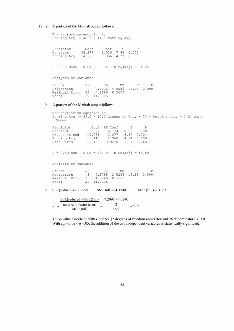
c. SSE(reduced) = 7.2998 SSE(full) = 4.3240 MSE(full) = .1663

SSE(reduced) - SSE(full) 7.2998 - 4.3240

number of extra terms 2 8.95MSE(full) .1663

F

The p-value associated with F = 8.95 (2 degrees of freedom numerator and 26 denominator) is .001.With a p-value < =.05, the addition of the two independent variables is statistically significant.



36

21. Decision Analysis

1. a. s1

s3

s2

s1

s3

s2

d 1

d 2

250

100

25

100

100

75

b. EV(d 1) = .65(250) + .15(100) + .20(25) = 182.5

EV(d 2) = .65(100) + .15(100) + .20(75) = 95The optimal decision is d 1

4. a. The decision to be made is to choose the type of service to provide. The chance event is the level of

demand for the Myrtle Air service. The consequence is the amount of quarterly profit. There are

two decision alternatives (full price and discount service). There are two outcomes for the chance

event (strong demand and weak demand).

b. EV(Full) = 0.7(960) + 0.3(-490) = 525

EV(Discount) = 0.7(670) + 0.3(320) = 565

Optimal Decision: Discount service

c. EV(Full) = 0.8(960) + 0.2(-490) = 670

EV(Discount) = 0.8(670) + 0.2(320) = 600

Optimal Decision: Full price service

7. a. EV(Small) = 0.1(400) + 0.6(500) + 0.3(660) = 538EV(Medium) = 0.1(-250) + 0.6(650) + 0.3(800) = 605EV(Large) = 0.1(-400) + 0.6(580) + 0.3(990) = 605

Best decision: Build a medium or large-size community center.

Note that using the expected value approach, the Town Council would be indifferent between building a medium-size community center and a large-size center.

b. The Town's optimal decision strategy based on perfect information is as follows:

If the worst-case scenario, build a small-size center If the base-case scenario, build a medium-size center If the best-case scenario, build a large-size center

Using the consultant's original probability assessments for each scenario, 0.10, 0.60 and 0.30, theexpected value of a decision strategy that uses perfect information is:

EVwPI = 0.1(400) + 0.6(650) + 0.3(990) = 727

In part (a), the expected value approach showed that EV(Medium) = EV(Large) = 605.



37

Therefore, EVwoPI = 605 and EVPI = 727 - 605 = 122

The town should seriously consider additional information about the likelihood of the threescenarios. Since perfect information would be worth $122,000, a good market research study could

possibly make a significant contribution.

c. EV(Small) = 0.2(400) + 0.5(500) + 0.3(660) = 528

EV(Medium) = 0.2(-250) + 0.5(650) + 0.3(800) = 515EV(Large) = 0.2(-400) + 0.5(580) + 0.3(990) = 507

Best decision: Build a small-size community center.

d. If the promotional campaign is conducted, the probabilities will change to 0.0, 0.6 and 0.4 for theworst case, base case and best case scenarios respectively.

EV(Small) = 0.0(400) + 0.6(500) + 0.4(660) = 564EV(Medium) = 0.0(-250) + 0.6(650) + 0.4(800) = 710EV(Large) = 0.0(-400) + 0.6(580) + 0.4(990) = 744

In this case, the recommended decision is to build a large-size community center. Compared to the

analysis in Part (a), the promotional campaign has increased the best expected value by $744,000 -605,000 = $139,000. Compared to the analysis in part (c), the promotional campaign has increasedthe best expected value by $744,000 - 528,000 = $216,000.

Even though the promotional campaign does not increase the expected value by more than its cost($150,000) when compared to the analysis in part (c), it appears to be a good investment. That is, iteliminates the risk of a loss, which appears to be a significant factor in the mayor's decision-making

process.



12. a.

9d 2

s1

s2

s3

7000

2000

-9000

8d 1

s2

s3

3500

2000

-1500

s1

4Cold

7d 2

s1

s2

s3

7000

2000

-9000

6d 1

s1

s2

s3

3500

1000

-15003 No rm al

2Wait

Don't Wait

11d 2

s1

s2

s3

7000

2000

-9000

10d 1

s1

s2

s3

3500

2000

-15005

1

b. Using Node 5,EV (node 10) = 0.4(3500) + 0.3(1000) + 0.3(-1500) = 1250EV (node 11) = 0.4(7000) + 0.3(2000) + 0.3(-9000) = 700

Decision: d 1 Blade attachment Expected Value $1250 (at Node 5)

c. EVwPI = 0.4(7000) + 0.3(2000) + 0.3(-1500) = $2950EVPI = $2950 - $1250 = $1700

d. EV (node 6) = 0.35(3500) + 0.30(1000) + 0.35(-1500) = 1000EV (node 7) = 0.35(7000) + 0.30(2000) + 0.35(-9000) = -100EV (node 8) = 0.62(3500) + 0.31(1000) + 0.07(-1500) = 2375EV (node 9) = 0.62(7000) + 0.31(2000) + 0.07(-9000) = 4330EV (node 3) = Max(1000,-100) = 1000 d 1 Blade attachment

EV (node 4) = Max(2375,4330) = 4330 d 2 New snowplow

The expected value of node 2 isEV (node 2) = 0.8 EV(node 3) + 0.2 EV(node 4)

= 0.8(1000) + 0.2(4330) = 1666EV (node 1) = Max(node 2, node 5) = Max(1666,1250) = $1666 Wait

The optimal strategy is“Wait until September and then,

If normal weather, choose the blade attachment, but if unseasonably cold, choose snowplow”

1

Date post:	04-Apr-2018
Category:	Documents
Upload:	zahra-ahmed-alfaraj
View:	219 times
Download:	0 times

Homework Solutions 10 e

Documents