Horizontal Pressure Gradients

• Pressure changes provide the push that drive ocean currents

• Balance between pressure & Coriolis forces gives us geostrophic currents

• Need to know how to diagnose pressure force

• Key is the hydrostatic pressure

Horizontal Pressure Gradients

• Two stations separated a distance x in a homogeneous water column ( = constant)

• The sea level at Sta. B is higher than at Sta. A by a small distance z

• Hydrostatic relationship holds

• Note, z/x is very small (typically ~ 1:106)

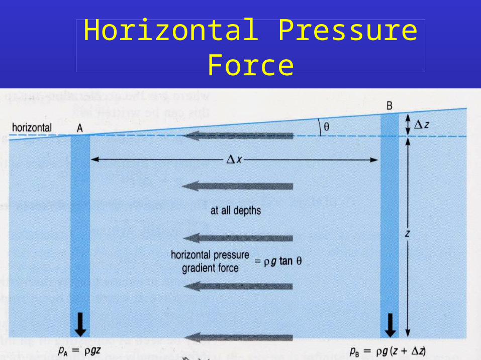
Horizontal Pressure Force

Pressure Gradients

@ Sta A seafloor ph(A) = g z

@ Sta B seafloor ph(B) = g (z + z)

p = ph(B) - ph(A) = g (z + z) - g z

p = g z

HPF p/x = g z/x = g tan

or HPF per unit mass = g tan[m s-2]

Horizontal Pressure Force

Geostrophy

• What balance HPF?

• Coriolis!!!!

Geostrophy

• Geostrophy describes balance

between horizontal pressure &

Coriolis forces

• Relationship is used to diagnose

currents

• Holds for most large scale motions

in sea

Geostrophic Relationship

• Balance: Coriolis force = 2 sin u = f u HPF = g tan

• Geostrophic relationship:

u = (g/f) tan

• Know f (= 2 sin) & tan, calculate u

f = Coriolis parameter (= 2 sin)

Estimating tan

• Need to slope of sea surface to get at surface currents

• New technology - satellite altimeters - can do this with high accuracy

• Altimeter estimates of sea level can be

used to get at z/x (or tan) & ugeo

• Later, we’ll talk about traditional method

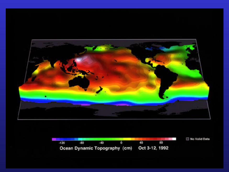
Satellite Altimetry

Satellite Altimetry

Satellite Altimetry

• Satellite measures distance between it and ocean surface

• Knowing where it is, sea surface height WRT a reference ellipsoid is determined

• SSHelli made up three important parts

SSHelli = SSHcirc + SSHtides + Geoid

• We want SSHcirc

Modeling Tides

• Tides are now well modeled in

deep water SSHtide =

f(time,location,tidal component)

• Diurnal lunar O1 tide

The Geoid

• The geoid is the surface of constant gravitational acceleration

• Varies in ocean by 100’s m due to differences in rock & ocean depth

• Biggest uncertainty in

determining SSHcirc

The Geoid

Groundtracks

• 10 day repeat orbit

• Alongtrack 1 kmresolution

• Cross-track 300 kmresolution

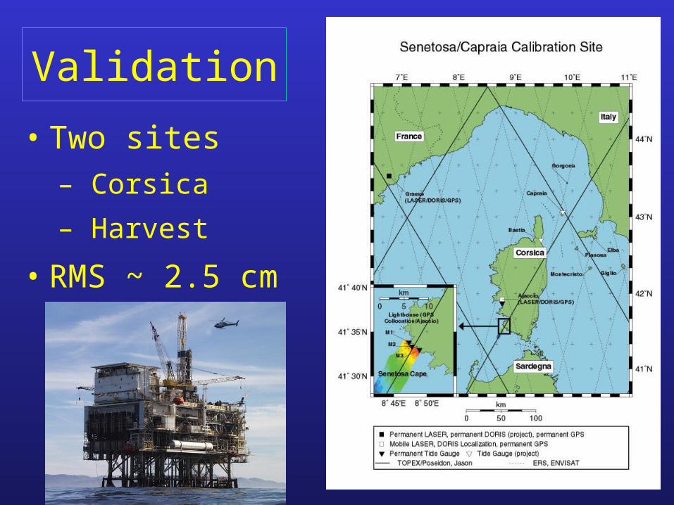
Validation

• Two sites– Corsica

– Harvest

• RMS ~ 2.5 cm

Mapped SSH

• SSH is optimally interpolated

• Cross-shelf SSH SSH ~20 cm over ~500 km

• tan = z/x

~ 0.2 / 5x105 or

~ 4 x 10-7

Geostrophic Relationship

• Balance: Coriolis force = fu HPF = g tan

• Geostrophic relationship:

u = (g/f) tan

• Know f (= 2 sin) & tan,

calculate u

Calculating Currents

• Know tan = 4x10-7

• Need f (= 2 sin)

– = ~37oN

– f = 2 (7.29x10-5 s-1) sin(37o) = 8.8x10-

5 s-1

• u = (g/f) tan = (9.8 m s-2 / 8.8x10-5 s-1) (4x10-

7) = 0.045 m/s = 4.5 cm/s !!

Mapped SSH

• u = 4.5 cm/s

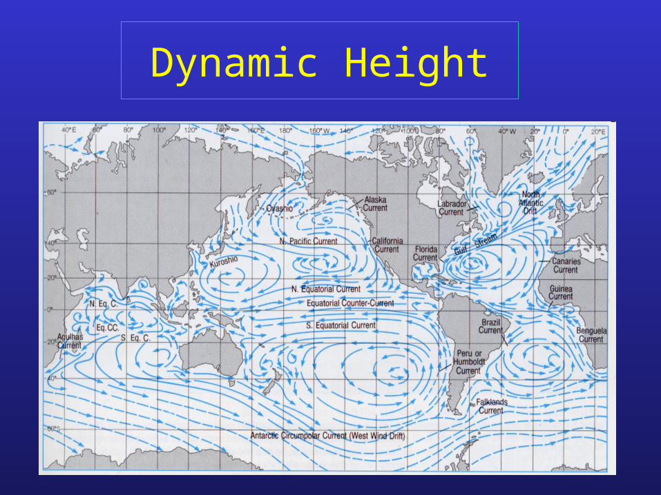
• Direction is along’s in SSH

• The California Current

Geostrophy

• Geostrophy describes balance between

horizontal pressure & Coriolis forces

• Geostrophic relationship can be used

to diagnose currents - u = (g/f) tan

• Showed how satellite altimeters can

be used to estimate surface currents

• Need to do the old-fashion way next

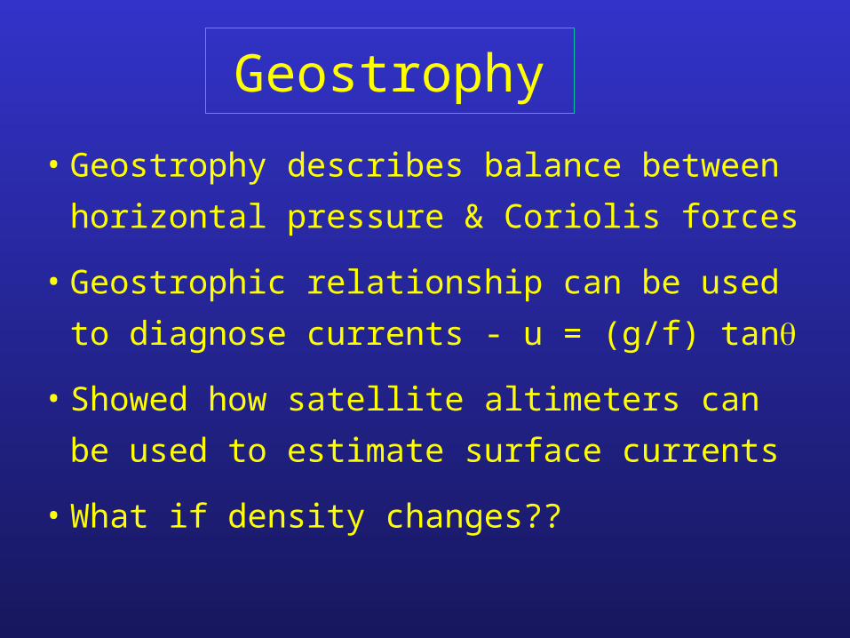
Geostrophy

• Geostrophy describes balance between

horizontal pressure & Coriolis forces

• Geostrophic relationship can be used

to diagnose currents - u = (g/f) tan

• Showed how satellite altimeters can be

used to estimate surface currents

• What if density changes??

Our Simple Case

Here, tan & u are = constant WRT depth

Barotropic Conditions

• A current where u f(z) is

referred to as a barotropic current

• Holds for = constant or when

isobars & isopycnals coincide

• Thought to contribute some, but not

much, large scale kinetic energy

Barotropic Conditions

Isobars & Isopycnals

• Isobars are surfaces of constant

pressure

• Isopycnals are surfaces of constant

density

• Hydrostatic pressure is the weight (m*g)

of the water above it per unit area

• Isobars have the same mass above them

Isobars & Isopycnals

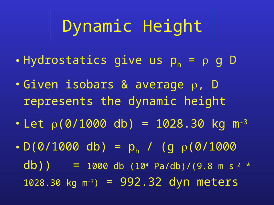
• Remember the hydrostatic relationship

ph = g D

• If isopycnals & isobars coincide then

D, the dynamic height, will be the same

• If isopycnals & isobars diverge, values

of D will vary (baroclinic conditions)

Baroclinic Conditions

Baroclinic vs. Barotropic

• Barotropic conditions

– Isobar depths are parallel to sea surface

– tan = constant WRT depth

– By necessity, changes will be small

• Baroclinic conditions

– Isobars & isopycnals can diverge

– Density can vary enabling u = f(z)

Baroclinic vs. Barotropic

Baroclinic vs. Barotropic

Baroclinic Flow• Density differences drive HPF’s -> u(z)

• Hydrostatics says ph = g D

• Changes in the mean above an isobaric surface will drive changes in D (=z)

• Changes in D (over distance x) gives tan to predict currents

• Density can be used to map currents following the Geostrophic Method

Baroclinic Flow

• Flow is along

isopycnal surfaces

not across

• “Light on the

right”

• u(z) decreases with

depth

Geostrophic Relationship

• Balance: Coriolis force = fu HPF = g tan

• Will hold for each depth

• Geostrophic relationship:

u(z) = (g/f) (tan(z))

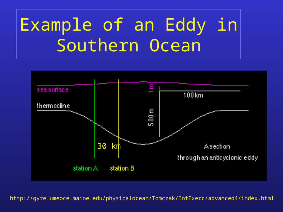
Example as a f(z)

A B

Goal: 1 or z1

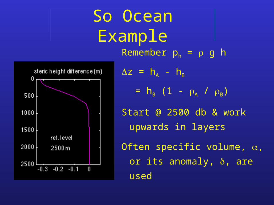
Example as a f(z)

• Define pref - “level of no motion” =

po

• Know p1@A = p1@B

-> A g hA = B g hB

• z = hB - hA =

= hB - B hB / A

= hB ( 1 - B / A )

Example as a f(z)

u = (g/f) (z/x)

= (g/f) hB ( 1 - B / A ) / L

If A > B (1 - B/A)

(& u) > 0

If A < B (1 - B/A)

(& u) < 0

Density ’s drive u

Example as a f(z)

• Two stations 50 km apart along

45oN

• A(500/1000 db) = 1028.20 kg m-3

B(500/1000 db) = 1028.10

kg m-3

• What is z, tan & u at 500 m??

Example as a f(z)

• z = hB - hA = hB ( 1 - B / A )

• Assume average distance (hA) ~ 500 m

• z = (500 m) (1 - 1028.10/1028.20)

= 0.0486 m = 4.86 cm

• tan = z / L = (0.0486 m)/(50x103 m)

= 9.73x10-7

Example as a f(z)

• u(z) = (g/f) (tan(z))

• f = 2 sin = 2 (7.29x10-5 s-

1) sin(45o) = 1.03x10-4 s-1

• u = (9.8 m s-2/1.03x10-4 s-1)

(9.73x10-7) = 0.093 m s-1

= 9.3 cm s-1

Geostrophy as a f(z)

• u = (g/f) hB ( 1 - B / A ) / L

• This can be repeated for each level

• Assumes level of no motion

• Calculates only the portion of flow perpendicular to density section

• Calculates only baroclinic portion of flow

Level of No Motion

• Level of no motion assumption

misses the barotropic part of

u(z)

Example of an Eddy in Southern Ocean

http://gyre.umeoce.maine.edu/physicalocean/Tomczak/IntExerc/advanced4/index.html

30 km

So Ocean Example

So Ocean Example

Remember ph = g h

z = hA - hB

= hB (1 - A / B)

Start @ 2500 db & work

upwards in layers

Often specific volume, ,

or its anomaly, , are

used

So Ocean Example

• u(z) = (g/f) tan (z)

• Adjust level of known motion

Dynamic Height

• Hydrostatics give us ph = g D

• Given isobars & average , D represents the dynamic height

• Let (0/1000 db) = 1028.30 kg m-3

• D(0/1000 db) = ph / (g (0/1000

db)) = 1000 db (104 Pa/db)/(9.8 m s-2 *

1028.30 kg m-3) = 992.32 dyn meters

Surface Currents from Hydrography

• Only the baroclinic portion of

the current is sampled

• Need a level of no/known motion

• Need many, many observations

• Can get vertical structure of

currents

Dynamic Height

• Dynamic height anomaly, D(0/1500db)

Dynamic Height

Surface Currents from Hydrography

Surface Currents from Altimetry

• Satellite altimeters can estimate

the slope of the sea surface

• Both barotropic & baroclinic

portions of current are

determined

• Only surface currents are

determined

Surface Currents from Altimetry

Dynamic Height

• California Cooperative Fisheries Investigations (CalCoFI)

• Understand ocean processes in pelagic fisheries

• Started in 1947

Dynamic Height

• January 2000 - CalCoFI Cruise 0001

Dynamic Height

• D(0/500db)

• Shows CA Current

• Recirculation in the SoCal Bight

Geostrophy

• Barotropic vs. baroclinic flow

• Flow is along lines of constant

dynamic height (light on the

right)

• Baroclinic portion can be

diagnosed from CTD surveys

• Quantifies the circulation of

upper layers of the ocean