Household Interaction and the Labor Supply of Married Women * Zvi Eckstein 1 and Osnat Lifshitz 2 October 2011 Draft Abstract The major increase in the employment rate of married women while that of men remained almost unchanged is one of the most dramatic socioeconomic changes to have taken place during the last century. In this paper, we argue that shifts in social norms regarding household interaction in determining a married couple’s labor supply can provide an explanation. Specifically, we formulate and estimate a dynamic discrete-choice labor supply model, assuming that there are two types of households – Classical and Modern. The Classical household follows a Stackelberg leader game in which the wife’s labor supply decision follows her husband’s already-known employment outcome. The Modern family is characterized by a symmetric and simultaneous game that determines their joint labor supply and has a Nash equilibrium. The family type – Modern or Classical – is exogenously determined when the couple gets married but is not observable for estimation. The model is estimated using the Simulated Moments Method (SMM) and data from the Panel Study of Income Dynamics (PSID) survey for the years 1983-93. The estimated model accurately predicts employment rates and produces a good fit of mean wages to the data. We estimate that 38 percent of families are Modern and that the participation rate of women in those households is almost 80 percent. The employment rate of women in Classical families is 10 percent lower than that while the employment rates of men is almost identical in the two household types. These results support our hypothesis that part of the increase in labor supply of married women may be due to an increase in the share of Modern families in the population. Keywords: dynamic discrete choice, household labor supply, household game JEL: E24, J2, J3 * This paper is based on Osnat Lifshitz’ PhD dissertation (2004) and the Walras-Bowley Lecture given at the Econometric Society Meeting, June 19, 2008 in Pittsburgh, USA. We have benefited from comments on earlier drafts made by Ellen McGratten, Jean-Marc Robin, Richard Rogerson and Ken Wolpin. We wish to thank Tali Larom for her research assistance. We are grateful for financial support from The Pinhas Sapir Center for Development, Tel Aviv University. 1 Tel Aviv University, IDC (Herzliya), CEPR and IZA; [email protected]2 Tel Aviv-Jaffa Academic College; [email protected]
Transcript
Household Interaction and the Labor Supply of
Married Women*
Zvi Eckstein1 and Osnat Lifshitz
2
October 2011
Draft
Abstract
The major increase in the employment rate of married women while that of men remained almost unchanged is one of the most dramatic socioeconomic changes to have taken place during the last century. In this paper, we argue that shifts in social norms regarding household interaction in determining a married couple’s labor supply can provide an explanation. Specifically, we formulate and estimate a dynamic discrete-choice labor supply model, assuming that there are two types of households – Classical and Modern. The Classical household follows a Stackelberg leader game in which the wife’s labor supply decision follows her husband’s already-known employment outcome. The Modern family is characterized by a symmetric and simultaneous game that determines their joint labor supply and has a Nash equilibrium. The family type – Modern or Classical – is exogenously determined when the couple gets married but is not observable for estimation. The model is estimated using the Simulated Moments Method (SMM) and data from the Panel Study of Income Dynamics (PSID) survey for the years 1983-93. The estimated model accurately predicts employment rates and produces a good fit of mean wages to the data. We estimate that 38 percent of families are Modern and that the participation rate of women in those households is almost 80 percent. The employment rate of women in Classical families is 10 percent lower than that while the employment rates of men is almost identical in the two household types. These results support our hypothesis that part of the increase in labor supply of married women may be due to an increase in the share of Modern families in the population. Keywords: dynamic discrete choice, household labor supply, household game
JEL: E24, J2, J3
* This paper is based on Osnat Lifshitz’ PhD dissertation (2004) and the Walras-Bowley Lecture given at the Econometric
Society Meeting, June 19, 2008 in Pittsburgh, USA. We have benefited from comments on earlier drafts made by Ellen McGratten, Jean-Marc Robin, Richard Rogerson and Ken Wolpin. We wish to thank Tali Larom for her research assistance. We are grateful for financial support from The Pinhas Sapir Center for Development, Tel Aviv University. 1 Tel Aviv University, IDC (Herzliya), CEPR and IZA; [email protected] 2 Tel Aviv-Jaffa Academic College; [email protected]
2
1 Introduction
Female employment and participation rates increased dramatically during the last century, with far-
reaching social and economic implications. While the employment rate of married women more than
doubled during the last fifty years, from 30 percent in 1962 to 62 percent in 2007 (Figure 1), the
employment rate among unmarried women (single, divorced and widowed) remained almost constant at
about 70 percent.3 Furthermore, the employment and participation rates of males, whether married or
unmarried, remained almost constant during the same period and exceeded those of comparable
females. It would appear therefore that changes in family behaviour must be taken into account in order
to understand female employment trends.
The dramatic change in employment rates among married women by age for the period 1962- 2007
can be seen in Figure 2 for the 1925 to 1975 cohorts.4 The graph clearly shows that married female
employment increased for all ages between the early cohorts and the baby boomers of 1945. The 1965
and 1975 cohorts show almost the same employment rate by age, though during the intervening years
female employment increased among younger women (Buttet and Schoonbroodt, 2005). The changes
by cohort are attributed in the literature to observables variables, such as schooling, wages, fertility and
marital status, as well as to changes in social norms, technological progress and other factors.
In this paper, we postulate an additional interpretation of the observed changes in the labor supply
of married men and women. It is hypothesized that married couples are divided into two alternative
types of households according to exogenously given social norms. Thus, the first type of household,
which we call “Classical” (C), is characterized by an intra-family dynamic game in which the husband
plays the role of a Stackelberg leader who takes the first move in each period while the wife relates to
the husband's move as given. In the other type of household, which we call “Modern” (M), the couple’s
dynamic decisions are simultaneous and symmetric and the outcomes are determined according to a
standard Nash equilibrium. The Classical household interaction follows Becker's approach in which
females take their husband’s labor supply as given. The Modern household interaction is based on the
casual observation that such households are made up of two "independent" individuals. In addition, our
aim is that female employment rates would be higher in a Modern household than in a comparable
Classical household.5 In the estimation, we assume that the type of household is unobserved with a
3 This fact is well known and is documented by Barton, Layard and Zabalza (1980), Coleman and Pencavel (1993) and
Mincer (1993). 4 For simplicity and in order to have a large enough sample for each cohort, we define the women born between, for example, 1953 and 1957, as the "1955 cohort" and similarly for the entire CPS data set. 5 Household games have been analyzed by Brown and Manser (1980) and McElroy and Horney (1981), Chiappori (1997) and
recently by many others. There are only a few empirical papers that use family games (Brown and Flinn, 2007 and Tartari, 2005). More recently, Del Boca and Flinn (2010) analyzed and estimated a static couple game of labor supply and showed that Nash equilibrium may be a preferred outcome relative to a cooperative specific game.
3
given probability. As a result, the model can be used to estimate the effect of a change in the proportion
of Modern households, which we attribute to changing social norms, on female employment.
The model consists of three endogenous labor market states: employment, unemployment and out
of the labor force. Wage offers are given exogenously as a random outcome that follows a logit
probability function and wage levels follow the standard Mincer/Ben-Porath wage equation.
Households are characterized by a common budget constraint and joint consumption where children
consume a proportional share and are added randomly depending on the state of the household. Divorce
is a potential exogenous event that occurs randomly, conditional on the household state.
We estimate the model using the Simulated Moments Method (SMM) and a PSID sample of 863
married couples who got married in 1983-4, for whom there is at most ten years of quarterly data. In
order to focus on internal family interactions, we assume that all parameters are the same for both types
of household. The estimated model provides a good fit to the trends in employment, unemployment,
wages and other parameters of household labor supply and the estimated parameters are consistent with
the theory and results presented in the literature. According to the results, the estimated employment
rate of women in Modern households exceed that of women in Classical households by 10 percent,
while the employment rate of men in each type of household is about the same. Since men have higher
job-offer rates and higher potential wages, they have broader employment choices in both types of
household. However, given the simultaneous choices in Modern households and the higher level of risk
aversion among women, more women in Modern households choose to participate in the workforce and
they also work more than their counterparts in Classical households.
An increase in the proportion of Modern households can provide an additional explanation for the
increase in female labor supply and is consistent with the argument that changes in culture are
responsible for the increase (see, Fernandez, 2007). In Eckstein and Lifshitz (2011), we found that only
62 percent of the increase in female labor supply among the 1925-1975 cohorts could be explained by
observable characteristics (i.e. schooling, wages, children, divorce and marriage rates). The main
factors proposed to account for this large unexplained portion are changes in the utility/cost of home
production and the cost of bearing and raising children.6 In Eckstein and Lifshitz (2011), we measured
6 The rapid technological progress in household production is the prime reason for the increase in female labor supply,
according to Greenwood et al. (2005) and Greenwood and Seshadri (2005). Their main argument is that the introduction of labor-saving appliances associated with technological progress in the home sector may have enabled more women to enter the workforce. They also argue that the time spent on housework fell from 58 hours per week in 1900 to just 18 hours in 1975, thus making it much easier for married women with children to enter the workforce. Albanesi and Olivetti (2007) claimed that until the early part of the 20th century, women spent more than 60 percent of their prime years either pregnant or nursing. From 1920 until 1960, improved medical knowledge, advances in obstetric practices and the introduction of infant formula have reduced the time-cost associated with raising children and led to an increase in participation by married women with children. Attanasio, Low and Sanchez-Marcos (2008) studied the lifecycle labor supply of three cohorts of American women born in the 1930s, 1940s and 1950s. They found that the combination of a reduction in the cost of children and a narrowing of the gender wage gap can explain the increase in the labor supply of mothers.
4
the magnitude of these changes that would account for the unexplained portion of the rise in
employment rates of married women.
The rest of the paper is organized as follows: The next section presents a dynamic household labor
supply model. Section 3 describes the PSID data and the estimation method. Section 4 presents the
estimation results and the fit to the data. Section 5 discusses counterfactuals of the model and Section 6
concludes.
2 The Model
We assume that from the point in time at which a couple marries (t = 0), their household is being
categorized as either "Classical" (C) or "Modern" (M),7 which are treated as two unobserved types. The
model solves for the labor supply of both the husband and wife. We assume that each period is divided
into two sub-periods: during the first sub-period, an individual who is out of the labor force (OLF) or
unemployed (UE) decides whether or not to search for a job. If s/he chooses to search, s/he receives at
most one job offer and then decides whether or not to accept it. If s/he is initially employed (E), s/he
can choose between OLF and E or s/he may be fired and become unemployed. Thus, there are three
possible states during the second sub-period: E, UE and OLF.
In order to focus on the impact of the internal family game on household labor supply, we assume
that utility functions, wage functions and job-offer rate parameters differ between husband and wife but
are identical in both types of household. The empirical analysis must take into account that household
type is unknown to the researcher, but known to the household members themselves. Therefore, the
model is solved for each household twice during estimation - once for M and once for C - and then the
value of the objective function is calculated separately for each. Thus, unobserved heterogeneity
(Heckman and Singer, 1984) enters the model through the type of household and their respective intra-
household games.
In each period t, from the wedding day (t = 0) until retirement (t = T), each spouse chooses an
element a from her (his) choice set A, which contains at most three alternatives: employment (a = 1),
unemployment (a = 2) and being out of the labor force (a = 3). The choice variable a
tjd equals 1 if
7 As indicated, Del Boca and Flinn (2010) specify the intra-household game to be endogenous where the alternatives are a
cooperative or (inefficient) Nash equilibrium.
5
individual WHj ,= chooses alternative a at time t and zero otherwise, such that the three alternatives
are mutually exclusive, i.e. 13
1=∑ =
a
tjad for all t.
Consumption (x) is a joint family outcome and as a result the household budget constraint in each
period t, t=1,…,T is given by:
)2.1 ( .11
ttttHtHtWtW Ncxdydy ⋅+=⋅+⋅
wheretW
y andtH
y are the wages of the wife and husband, respectively and t
x is the couple's joint
consumption during period t. For simplicity, we define the cost per child (per-child consumption) in
goods and denote it as )(11
t
tHtHtWtW
N
dydy
tc⋅+⋅
⋅=θ , where θ is a given fraction of family income per child.8
tN is the number of children in the household, which is given by
tttnNN += −1 , where the event of
birth, 1=t
n , is a given random event that depends on employment and other states of the household.
We adopt the Mincerian/Ben-Porath wage function for each j = H,W where experience is
endogenously determined, such that:
.ln 14
213121 jtj
j
jt
j
jt
jj
tj SKKy εββββ ++++= −− (2.2)
where jtK 1− is actual work experience accumulated by the individual according to
1
1 tjjttj dKK += − , for
which the initial value is the level of experience on the day of the wedding and j
S denotes the
predetermined individual's years of schooling. jt
ε is the standard zero-mean, finite-variance and
serially independent error, which is uncorrelated with K and S.
Utility from consumption is given by a constant relative risk aversion and utility from leisure and
children is linear, such that, 9
)2.3( ( ) ( ),ttjjtjtj NflxuU +⋅+= α
where ( ) ( )
j
jtx
tj xu γ
γ
= is utility from total household consumption, tjl is the individual's leisure and ( )tNf is
a specific function for utility from children:
)2.4( ( ) [ ].1
20 t
tHtW
tN
ll
agettt cNNf+
++⋅= γγγ
Each parent's utility from their children increases with the number of children, with the given
consumption per child, ct,, and with the parents' total leisure per child, which decreases with the average
8 In order to keep the dynamic programing simple, we abstract from savings, although utility is not assumed to be linear. 9 We use the assumption that all earnings are consumed, i.e. neither saving nor borrowing is feasible. This assumption is extreme though standard in the modeling of dynamic labor supply.
6
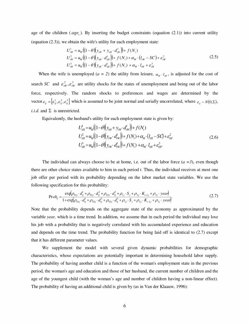
age of the children (t
age ). By inserting the budget constraints (equation (2.1)) into current utility
(equation (2.3)), we obtain the wife's utility for each employment state:
( )( )( )( )( )( ) ( )
( )( )( ) 313
212
11
)(1
)(1
)(1
tWtWWttHtHWtW
tWtWWttHtHWtW
ttHtHtWWtW
lNfdyuU
SClNfdyuU
NfdyyuU
εαθ
εαθ
θ
+⋅++⋅−=
+−⋅++⋅−=
+⋅+−=
(2.5)
When the wife is unemployed (a = 2) the utility from leisure, tWW
l⋅α , is adjusted for the cost of
search SC and 32 ,tWtWεε are utility shocks for the states of unemployment and being out of the labor
force, respectively. The random shocks to preferences and wages are determined by the
vector [ ]321 ,, tjtjtjtj εεεε = which is assumed to be joint normal and serially uncorrelated, where ( )Σ,0~ Ntjε ,
i.i.d. and Σ is unrestricted.
Equivalently, the husband's utility for each employment state is given by:
)2.6(
( )( )( )( )( )( ) ( )
( )( )( ) .)(1
)(1
)(1
313
212
11
tHtHHttWtWHtH
tHtHHttWtWHtH
ttWtWtHHtH
lNfdyuU
SClNfdyuU
NfdyyuU
εαθ
εαθ
θ
+⋅++⋅−=
+−⋅++⋅−=
+⋅+−=
The individual can always choose to be at home, i.e. out of the labor force (a =3), even though
there are other choice states available to him in each period t. Thus, the individual receives at most one
job offer per period with its probability depending on the labor market state variables. We use the
following specification for this probability:
( )( )
.exp1
expPr
3121
3
03
2
02
1
01
3121
3
03
2
02
1
01
yearKSddd
yearKSdddob
jjtjjjtjjtjjtjj
jjtjjjtjjtjjtjj
tj⋅+⋅+⋅+⋅+⋅+⋅+
⋅+⋅+⋅+⋅+⋅+⋅=
−
−
ρρρρρρ
ρρρρρρ (2.7)
Note that the probability depends on the aggregate state of the economy as approximated by the
variable year, which is a time trend. In addition, we assume that in each period the individual may lose
his job with a probability that is negatively correlated with his accumulated experience and education
and depends on the time trend. The probability function for being laid off is identical to (2.7) except
that it has different parameter values.
We supplement the model with several given dynamic probabilities for demographic
characteristics, whose expectations are potentially important in determining household labor supply.
The probability of having another child is a function of the woman's employment state in the previous
period, the woman's age and education and those of her husband, the current number of children and the
age of the youngest child (with the woman’s age and number of children having a non-linear effect).
The probability of having an additional child is given by (as in Van der Klaauw, 1996):
7
(2.8) ( )( )tttHtW
HWH
t
W
t
W
ttt ageNddSSAGEAGEAGENN ⋅+⋅+++⋅+⋅+⋅+⋅+⋅Φ=+= − 981
71
6543
2
211 )1Pr( λλλλλλλλλ
where ( )⋅Φ is the standard normal distribution function. The probability of divorce is estimated as a
function of how long the couple has been married (t), the current number of children, the woman's
education and the employment states of both the woman and her husband:
( ).)1/0Pr( 1
6
1
543
2
211 tHtW
W
tttt ddSNttMM ξξξξξξ +⋅+⋅+⋅+⋅+⋅Φ=== − (2.9)
The dynamic programming solution to the optimization problem is obtained by a process of backward
recursion. In the terminal period T, we use a linear approximation of the value function in the final
period, as follows:
( ) ., 321 jjTjjjTTj SKTV ⋅+⋅+=Ω δδδ (2.10)
The solution for the first sub-period within each period depends on the household type. Therefore,
in what follows, we describe the solution of the game separately for each type of household.
2.1 The Classical Household (C) Labor Supply
The Classical household game is solved in three stages. In the first, the husband chooses whether or not
to search. Let ( )tHtHV Ω be the maximum expected discounted lifetime utility given the relevant state
space tHΩ , such that [ ]tttWtHWHtWtHtH ageNddSSkk ,,,,,,,=Ω . In this stage, the husband solves the
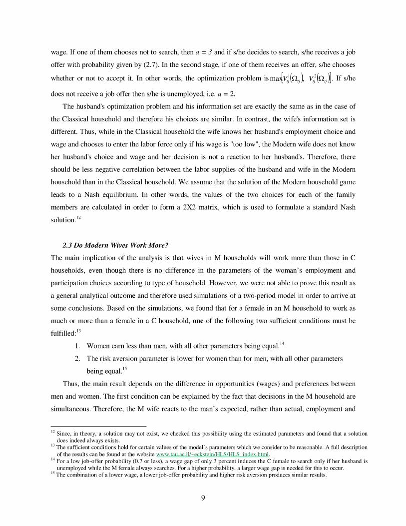
wage. If one of them chooses not to search, then a = 3 and if s/he decides to search, s/he receives a job
offer with probability given by (2.7). In the second stage, if one of them receives an offer, s/he chooses
whether or not to accept it. In other words, the optimization problem is ( ) ( )[ ]tjtjtjtj VV ΩΩ 21 ,max . If s/he
does not receive a job offer then s/he is unemployed, i.e. a = 2.
The husband's optimization problem and his information set are exactly the same as in the case of
the Classical household and therefore his choices are similar. In contrast, the wife's information set is
different. Thus, while in the Classical household the wife knows her husband's employment choice and
wage and chooses to enter the labor force only if his wage is "too low", the Modern wife does not know
her husband's choice and wage and her decision is not a reaction to her husband's. Therefore, there
should be less negative correlation between the labor supplies of the husband and wife in the Modern
household than in the Classical household. We assume that the solution of the Modern household game
leads to a Nash equilibrium. In other words, the values of the two choices for each of the family
members are calculated in order to form a 2X2 matrix, which is used to formulate a standard Nash
solution.12
2.3 Do Modern Wives Work More?
The main implication of the analysis is that wives in M households will work more than those in C
households, even though there is no difference in the parameters of the woman’s employment and
participation choices according to type of household. However, we were not able to prove this result as
a general analytical outcome and therefore used simulations of a two-period model in order to arrive at
some conclusions. Based on the simulations, we found that for a female in an M household to work as
much or more than a female in a C household, one of the following two sufficient conditions must be
fulfilled:13
1. Women earn less than men, with all other parameters being equal.14
2. The risk aversion parameter is lower for women than for men, with all other parameters
being equal.15
Thus, the main result depends on the difference in opportunities (wages) and preferences between
men and women. The first condition can be explained by the fact that decisions in the M household are
simultaneous. Therefore, the M wife reacts to the man’s expected, rather than actual, employment and
12 Since, in theory, a solution may not exist, we checked this possibility using the estimated parameters and found that a solution
does indeed always exists. 13 The sufficient conditions hold for certain values of the model’s parameters which we consider to be reasonable. A full description
of the results can be found at the website www.tau.ac.il/~eckstein/HLS/HLS_index.html. 14 For a low job-offer probability (0.7 or less), a wage gap of only 3 percent induces the C female to search only if her husband is
unemployed while the M female always searches. For a higher probability, a larger wage gap is needed for this to occur. 15 The combination of a lower wage, a lower job-offer probability and higher risk aversion produces similar results.
10
income outcome. However, in C households, the female knows her husband’s actual income and will
react only if the male ends up earning less than expected. In addition, men are expected to attain better
outcomes than women. Hence, women in M households more frequently make the choice to work. The
second condition implies that the more risk-averse wife in a simultaneous decision game (i.e. in an M
household) will work more than if she was reacting to her husband’s actual observed outcomes (as in a
C household).
3 Data and Estimation
The data is taken from the PSID (Panel Study of Income Dynamics) survey for the period 1983-93. We
use quarterly data which is available only from 1983 onward and restrict the model to the first ten years
of marriage.16 In order to create similar initial conditions for all individuals, we restrict the data to start
from the date of the wedding (as in the model) and consider all couples in the PSID sample who got
married during the period 1983-4. The data thus provides information on 863 couples and tracks them
until 1993 or until they separate. During the sample period, 36.3 percent of the couples divorced or
separated and 14.5 percent were removed from the sample for other reasons, such that after 10 years
49.2 percent of the couples remained in the sample.
The data includes demographic and employment information on individuals and households, such
as wages, working hours, unemployment (job search) and non-participation, as presented in Table 1.
Thus, the employment rate (participation rate) of the women in the sample increased from 67.8 percent
(72.1 percent) in 1984 to 77.4 percent (79.1 percent) after 10 years of marriage, while their
unemployment rate fell from 5.1 percent to 2.6 percent. The employment rate (participation rate) of the
men increased from 84.3 percent (92.6 percent) in 1984, to 89.9 percent (93.7 percent) in 1993 and the
unemployment rate decreased from 10 percent to 3.5 percent. During the ten-year period, the average
years of schooling and average hours of work remained unchanged. However, real monthly income
increased by a factor of 1.87 for men and 1.44 for women.
In order to determine whether the PSID sample is representative, we compared it to an equivalent
CPS sample, which is presented in the last column of Table 1. The CPS data is restricted to married
males and females who were interviewed in 1984 and had the same age distribution as the PSID
sample. The main difference between the samples is that the CPS consists of all individuals who were
married in 1984 while the PSID sample consists only of individuals who were newly married in that
year. While the husbands' characteristics and the wives' years of schooling are almost identical in both
16 We solve the recursive optimization backwards from the 11th year of marriage and it is assumed to be a parameterized function of
the state space in the 40th quarter with the terminal value function given by equation (2.10).
11
samples, the couples in the CPS sample have more children and wives' participation and employment
rates are lower. This is not surprising, given the shorter time that couples in the PSID sample have been
married.
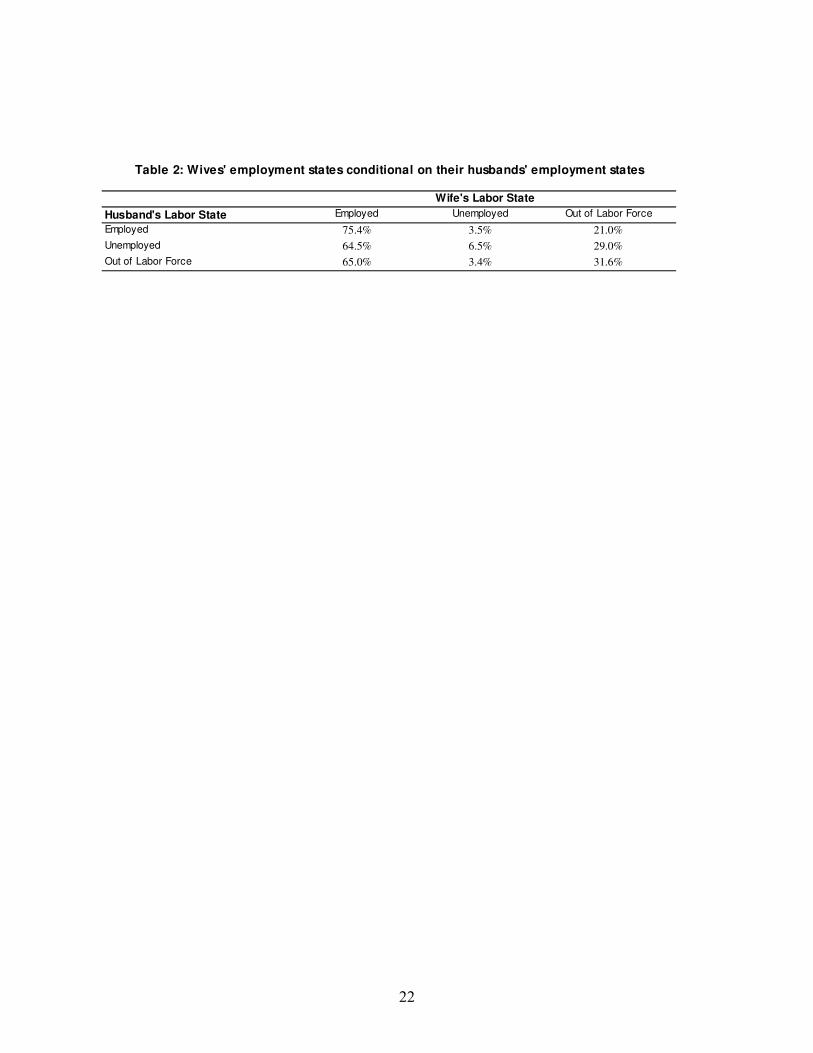
Table 2 presents the employment states of wives conditional on their husbands' labor market state.
It is interesting to note that the employment rate (out of the labor force rate) among women is 75.4
percent (21 percent) if their husband is working but only about 65 percent if he is unemployed or out of
the labor force. In other words, a woman is more likely to be employed if her husband is employed than
if he is unemployed or out of the labor force. To account for this in a model where both spouses
endogenously determine their labor supply is an additional challenge to be dealt with.
Estimation
Estimation involves solving the model twice for each household, i.e. once for M households and
once for C households, where the value of the objective function is calculated separately for each
member of each type of household.17 We treat the probabilities of the two types of household according
to the standard non-parametric probability of constant proportions, πM + πC = 1 (see Heckman and
Singer, 1984).
The model is estimated using SMM (Simulated Method of Moments) following Pakes and Pollard
(1989). Let i
T be the length of time we observe household i and let θ be the vector of parameters,
including Σ. We denote the data on actual choices made by the husband and wife in household i as
),;,...,1;( HWjTtd i
o
itj == and the predicted choices for family type h = M, C as
( ) ),;,...,1;,( HWjTthd i
p
itj ==θ . We define:
( ) ( )
( ) otherwiseD
hddifD
h
itj
p
itj
o
itj
h
itj
1
,0
=
==
θ
θθ.
( )θh
itjD equals zero if the model correctly predicts the choice of individual j in household i in
period t under the specification of family type h and one otherwise. Hence, ( )θh
itjD is a matrix of
moments that includes the predicted and observed transition probabilities. The sum of these elements is
the first moment to be minimized and is given by:
)(D)(g863
1i
T
1t W,Hj
h
itj
h
1
i
θθ ∑∑ ∑= = =
= .
17 In the model, we assume that the household type probability is a given parameter. In analyzing the results, we use the
estimated model to correlate the posterior probability of each family with observables (Eckstein and Wolpin, 1999).
12
We define the weighted vector of the two household types according to the assumed proportions,
Cπ and
C1 π− , as:
( ) ( ) ( )')1('', 111 θπθππθ M
C
C
CC ggg −+=
We denote the actual wage of the individual as ),;,...,1;( HWjTtw i
o
itj == and the predicted
equivalent for a household of type h as ( ) ),;,...,1;,( HWjTthw i
p
itj ==θ . The second set of moments is
based on the difference between observed and predicted wages. Specifically, we calculate the squared
difference between the average over households of the observed and predicted weighted wage per
household in each quarter t for H and W separately. The average weighted wage of the two household
types is ( ) ( ) ( )θπθππθ ,)1(,, MwCwwp
tjC
p
tjCC
p
tj −+= .
Let ( )',2 Cg πθ be the vector of these 80 moments as follows:
( ) ( )( ) ( )( ) ( )( ) ( )( )[ ]2
4040
2
11
2
4040
2
112 ,,...,,,,,...,,', C
p
W
o
WC
p
W
o
WC
p
H
o
HC
p
H
o
HC wwwwwwwwg πθπθπθπθπθ −−−−= .
We define the vector of moments as ( ) ( ) ( )[ ]',,,', 21 CCC ggg πθπθπθ = .
The SMM is defined by the minimum of the objective function:
),g( W)',g( ),J( CCC πθπθπθ =
with respect to θ and C
π , where the weighting matrix W is a diagonal matrix. The weight assigned to
each moment is the inverse of the estimated standard deviation of the specific moment in the data. We
find the estimated standard errors using the inverse of the Jacobian matrix.
4 Results
This section presents the SMM estimation results for the model. We first ask whether there are indeed
two types of household. Or do all households Classical? The estimated proportion of Classical
households is 0.61 with standard error of 0.027 (see Table 3). Furthermore, estimating the model by
assuming that all households solve the Classical game increases the J value from 47.22 to 361.9 and
assuming that all households solve the Modern game increases the J value to 693.3. Hence, using the
standard test statistic (Newey and West, 1987) we reject the hypothesis that all households follow the
Classical game or the Modern game in determining the couple’s labor supply.18
In what follows, we first look at how well the estimated model fits the observed average
employment states, the transitions between states and average wages by gender, conditional on the
18 It should be noted that one could allow for a more flexible form of Classical game (e.g., unobserved heterogeneity in utility
and other parameters) in which case the hypothesis of a zero proportion of Modern households may not be rejected.
13
estimated parameters. Given that the model provides a satisfactory fit to the data, we then interpret the
estimated parameters. This then facilitates an analysis of the estimated model’s counterfactual
predictions (both within-sample and out-of-sample) for the labor supply of Classical and Modern
households.
Goodness of Fit
The estimated parameters and assumed random errors were used to calculate the predicted proportions
of the three labor market states in the sample. The calculations were done for all observed households
that were each classified as M or C and averaged using the estimated proportions of household type.
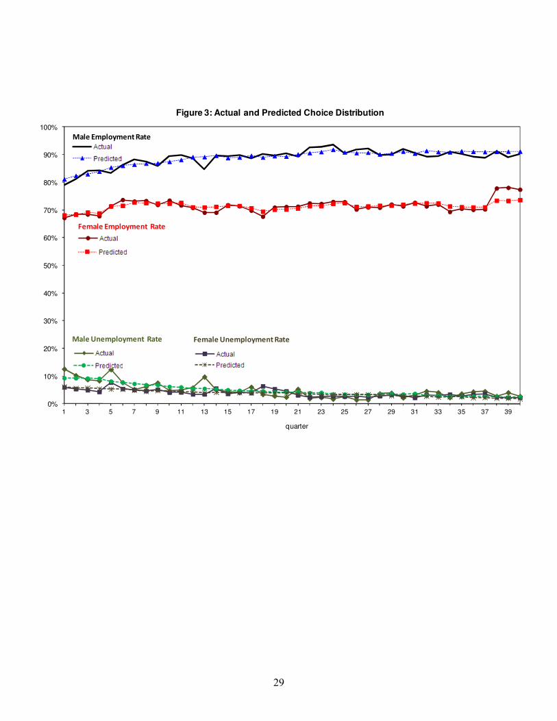
Figure 3 presents the actual and the predicted proportions of men and women in the states of
employment (E) and unemployment (UE). The estimated model provides a good fit to the aggregate
proportions and a simple goodness-of-fit test for each choice over the entire sample gives a value which
is under the critical 5 percent level for all cases, except UE for men.19 We also tested the goodness-of-
fit of actual to predicted choices for each of the 40 quarters of data and in 36 (29) of the 40 quarters, the
model passes the simple 2χ goodness-of-fit test for women (men).20 The model correctly predicts
45,925 of the 51,050 observed choices in the sample, which implies that the estimated model predicts
almost 90 percent (pseudo2
R ) of the choices made within the sample period.
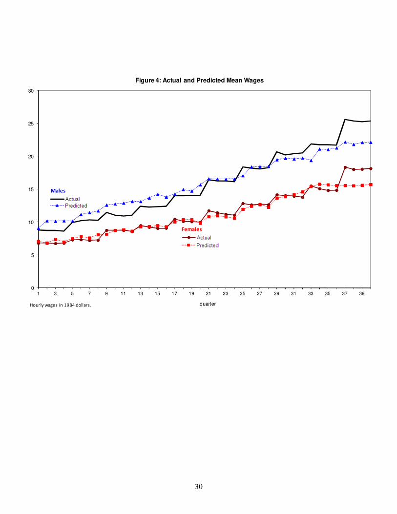
The model accurately predicts the trends and levels of actual wages for both females and males,
except for the large outlier in actual real wages in 1993, which is the last year of the sample (see Figure
4).21 Using a simple test for the equality of mean predicted wages for males and females we cannot
reject the hypothesis that estimated and actual means are equal for the entire sample. Using the same
test period by period, we reject the hypothesis for several periods, mainly for males.22 In Table 3, we
report the predicted distribution of the wives’ labor market states conditional on their husband’s, both in
the aggregate and by type of household. The predicted aggregate distribution is very similar to the
actual one presented in Table 2 and the estimated model successfully captures the positive correlation
between the labor supplies of a husband and wife. The correlation is stronger for Modern households
than for Classical households, as can be seen from Table 3.
19 The 2χ test statistics for employment, unemployment and out of the labor force are 6.18, 133.32 and 19.41 respectively for
males and 6.64, 47.34 and 25.97 respectively for females. The relevant critical value is 2χ (39) = 54.57. 20 See the above-mentioned website for the full results. 21 In the last year, there are only 425 observations. 22 For all periods, the t-test statistic is 0.44 for males and 1.43 for females. In separate tests for each period, for women, the
hypothesis is rejected for periods 38 and 37. For men, the hypothesis is rejected for periods 2-4, 6-12, 14-16, 20, 33 and 37-40.
14
Finally, it should be noted that the good fit of the estimated model to the data is not a complete
surprise since these moments were used for the SMM estimation criterion.
Parameters (Table 4)
Women are more risk averse than men as can be seen from the risk aversion parameter (Wγ = 0.849 for
women and Hγ = 0.948 for males).23 Furthermore, women attribute a higher value to leisure (home
production) than men (9.2 vs. 8.2). Labor search costs are positive and the joint family parameters of
utility from children (γ1 and γ2) have the expected signs (i.e. positive) and magnitudes.
Wages of both men and women increased substantially during the sample period (Figure 4). As a
result, the estimated experience parameters in the wage equation are large and higher for the husband
than for his wife. Interestingly, the estimated rate of return on a year of schooling is slightly lower for
the husband than for his wife (0.81 vs. 0.87). In the sample, men have slightly less years of schooling
than women (12.7 vs. 12.8) and as a result, the expected wage offer for a newlywed male is higher than
that for his newlywed wife unless she has significantly more years of schooling than he does, which is
unexpected given the assortive mating observed in the data (i.e. a correlation of 0.52 between the years
of schooling of husband and wife).
The job-offer probability parameters are higher for men than for women, apart from the state of
employment parameter (see Table 3).24 In particular, males have higher job offer rates when they are
unemployed and out of the labor force, and the time trend has a larger impact on them. In light of their
higher job offer rates and higher wage offers conditional on the labor market state, the job market
opportunities of husbands are superior to those of their wives.
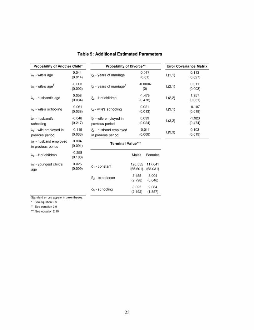
The parameters of the exogenous processes of having children and divorce have the predicted signs
(see Table 5). The probability of having another child decreases with number of children, parents’ level
of schooling and if the wife was employed in the previous quarter and increases with the ages of the
parents. The probability of divorce increases (at a decreasing rate) with years of marriage, the wife’s
years of schooling and if she was employed in the previous quarter. Terminal values, estimated
parameters and the estimated variance matrix of the three errors are presented in Table 5.
Employment by Type of Household
The estimated parameters are consistent with the assumption that the husband's labor market
opportunities and incentives are superior to his wife’s and therefore his search intensity is greater. As a
23 ( ) ( )
j
jtx
tj xu γ
γ
=
24 The other parameters are presented in Table 5.
15
result, the employment rate of husbands is much higher. As can be seen from Table 3, the wife in a
Classical household reacts to the outcome of her husband's search and thus is more likely to search if
her husband is unemployed or is out of the labor force. In the Modern household, the wife searches
simultaneously with her husband and, as a result of her risk aversion and the unknown outcome of her
husband’s search, searches more intensively. Thus, wives in the Modern household have a 10% higher
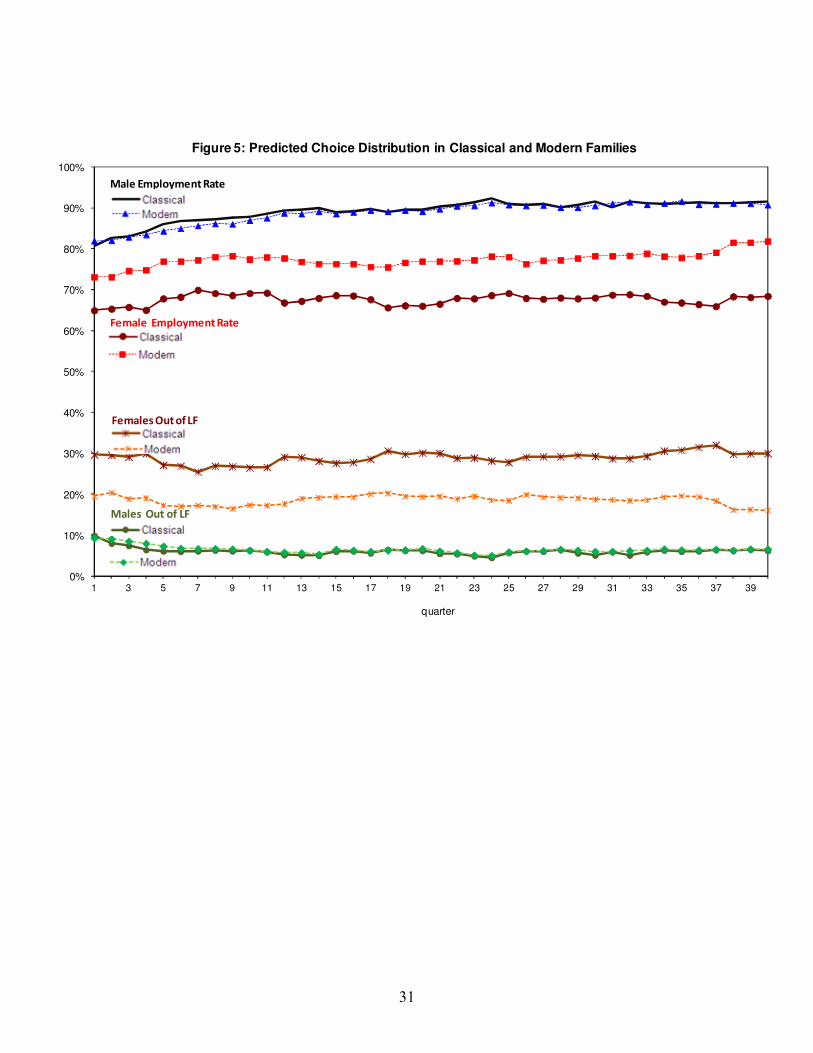
rate of employment than those in the C household.
The predicted rates of employment and unemployment for women differ significantly between M
and C households (see Figure 5). Thus, the employment rate of C women is on average 9.7 percent less
than that of M women and this gap remains almost constant over the sample period. The unemployment
rate for C women is 3.5 percent, which is 0.6 percentage points less than for M women. This is
primarily because C women search less intensively and therefore have a lower probability of not
finding a job and becoming unemployed. Simple chi-square tests indicate that employment state
distributions of C and M women are significantly different in all 40 quarters.25
By construction, all the parameters in the model are identical for the two types of households.
Hence, the differences in employment rates can only be due to which game the household plays. As
explained above, the main difference between the two types of households is that an M household
makes simultaneous decisions while the C household makes sequential decisions. This has implications
for the choices made by wives, in view of their risk aversion ( 850.W=γ ) and that employment serves
as insurance against a potential drop in consumption.
Male employment rates are similar in Modern and Classical households (88.7 percent versus 89.1
percent) and consequently their unemployment and out of the labor force rates are almost the same.
Chi-square tests showed that there are no significant differences in predicted employment rates between
husbands in C and M households in any of the 40 quarters.26 This result is due to two aspects of the
model and the estimated parameters: First, the husband has a very low estimated level of relative risk
aversion ( Hγ = 0.95), such that he is essentially indifferent to his wife’s impact on household
consumption. Hence, a potential change in a wife’s labor supply does not significantly affect the
husband's decisions in either type of household and therefore the game structure is irrelevant to the
husband's labor supply. Second, the male's decisions in both games are based on the same information
25 The 2χ test statistics for employment, unemployment and out of the labor force are 298.8, 28.9 and 1418.1 respectively for
women. The critical value is 2χ (39) = 54.57. 26 The 2χ test statistics for employment, unemployment and out of labor force are 2.1, 16.3 and 14.0 respectively for males.
The critical value is 2χ (39) = 54.57.
16
regarding female employment opportunities. Thus, even with a higher degree of risk aversion one
would expect that men’s employment outcomes would differ less by type of household than women’s.
One way to analyze the empirical content of the estimated unobserved household types is through
the correlation of the estimated type probability of each household conditional on the observed
employment outcomes (i.e. the posterior probability; see, for example, Eckstein and Wolpin, 1999) with
household demographic indicators, such as a husband with less than 12 years of schooling, an Afro-
American husband, a Protestant husband, residence in a rural area, etc. (see Table 6). Using standard
Bayesian conditional probability, we can calculate the probability for each household as to whether it is
playing a game of type C or type M. Table 6 shows that an M couple is more likely to be younger, to
have fewer children and to have a higher level of education and the head of the household is more likely
to be white and Catholic. In addition, the probability that an M couple stays married for 10 years is
lower than for a C couple. These results are consistent with our prior probabilities on the demographic
characteristics of modern and classical households and therefore our confidence in the model's
interpretation of the data is reinforced.
5 Counterfactuals
In this section, we use the estimated model to measure the potential increase in female employment due
to a change in the rules of the game, i.e. in social norms, which determine the household’s joint labor
supply. This is done through three simulations: in the first, we assume that all households are of type
C; in the second, we assume that all households are of type M and leave the employment opportunities
of men and women as estimated, with the goal of measuring the potential marginal impact on
employment; and finally, in the third, we in addition assume identical employment opportunities for
men and women in terms of wages and job-offer rates.
Simulation 1: All households are Classical (Figure 6)
In this simulation, we assume that 100 percent of the households in the population are classical rather
than the estimated proportion of 61.2 percent. As a result, the average predicted female employment
rate decreases to 0.676 from the estimated rate of 0.71 while the predicted male employment rate
remains almost the same (0.891 as compared to the estimated rate of 0.890). The decrease of 3.5% in
the employment rate is due to women with employed husbands who choose to work under the modern
specification, but choose not to search under the classical specification.
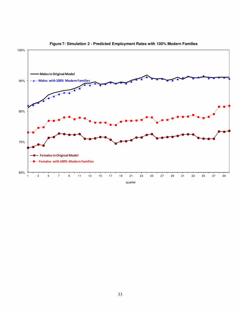
Simulation 2: All households are Modern (Figure 7)
17
In this simulation, we assume that 100 percent of the households in the population are Modern rather
than the estimated proportion of only 38.6 percent. As a result, the predicted female employment rate
increases to 0.77 from the estimated 0.71 while the predicted male employment rate remains almost the
same (0.887 as compared to the estimated rate of 0.890). According to the predicted outcome of the
simulation, even when the entire population consists of M households the male employment rate
exceeds that of women by 11.3 percentage points. This is due to the differences in wages, job-offer
probabilities and preferences, as explained above.
The results imply that changes in social norms over time, as represented by a change in the
proportions of M and C households for different cohorts, may have had a large impact on the
employment rate of married women, while hardly affecting married men. This potential result is
consistent with the data (Eckstein and Lifshitz, 2011).
Simulation 3: All households are Modern and employment opportunities for both genders are
identical (Figure 8)
In addition to the assumptions of Simulation 2, we now calibrate the female wage function and job-
offer probability parameters to the values estimated for men. As a result, the employment rate of
women increases to 0.84 and that of men decreases to 0.88. Thus, male and female employment rates
differ by only 3.2 percentage points in this case, which is due solely to differences in the utility function
parameters. For example, the value of leisure is higher for women ($10 dollars per hour for women as
compared to only $8.9 per hour for men). In addition, women have a higher level of relative risk
aversion (i.e. a lower γ ) than men, as discussed above. In other words, the marginal utility from
consumption is lower for women and therefore they require larger incentives to work outside the home.
Wages and job-offer rates are taken as exogenous here and we compare employment outcomes
when social norms based on an M-type game maximize employment rates of married women.
Obviously, in equilibrium the change in labor supply would affect wages and job-offer rates. However,
since we expect that preferences for leisure, consumption and household amenities differ between men
and women, we would also expect differences in the distribution of employment outcomes, as is the
case in a fully symmetric game like that in M households.
18
6 Concluding Remarks
A dynamic game model was estimated for household labor supply using PSID quarterly data on a
sample of married couples who were tracked for at most ten years. The model allows for the couple to
play one of two possible games: a standard game in which the husband is a Stakelberg leader who
makes his decisions first and the wife reacts to his outcomes and a Nash game in which husband and
wife play a simultaneous symmetric game. The households playing the former game are called
Classical and those playing the latter game are called Modern. We assume that household type is
distributed randomly and exogenously determined at the time of marriage. The model also assumes
dynamic stochastic arrival of children and divorce which affect the couple’s lifetime dynamic labor
supply.
The estimation results indicate that 61 percent of the 1983-4 cohort of newlywed couples are of the
Classical type and the hypothesis that all households are Classical is rejected. Furthermore, the
estimated labor market state outcomes and wages provide a very good fit to the data. We find that the
labor supply of men is not affected by the format of the game while the employment rate for women is
lower by about 10 percent in Classical households than in Modern households.
Taking the view that the format of the game played in the household is dependent on its
sociodemographic characteristics, we compute the posterior probabilities for each couple to be of a
particular type. We find that the Modern household is more likely to be young, better educated and
urban. In other words, the social norms reflected in a Nash symmetric game lead to an increase in the
labor supply of women in Modern households while leaving that of their husbands unchanged, which is
confirmed in the data. These results support the hypothesis that some of the increase in married female
labor supply observed in recent decades may be due to changes in social norms that affect the way
couples decide on their joint labor supply. To further investigate this hypothesis would require access to
additional data on, for example, couples who married at different points in time in order to determine
whether the proportions of household types is changing over time, as claimed here. Moreover,
additional specifications of the model, robustness tests and convincing dynamic games that determine
household labor supply are needed to further investigate whether changing social norms are an
important component in explaining the rise in labor supply of married women.
19
7 References
Albanesi, S. and C. Olivetti (2009), " Home Production, Market Production and the Gender Wage Gap:
Incentives and Expectations," Review of Economic Dynamics, Vol.12, No. 1: 80–107.
Albanesi, S. and C. Olivetti (2009a), "Gender Roles and Medical Progress," NBER Working Papers
14873.
Attanasio, O., H. Low, and V, Sánchez-Marcos (2008), “Explaining Changes in Female Labor Supply
in a Life-Cycle Model" The American Economic Review, Volume 98, Number 4:1517-
1552(36).
Barton, M., R. Layard and A. Zabalza (1980), “Married Women's Participation and Hours” Economica,
New Series, Vol. 47, No. 185: 51-72.
Becker, G. (1974), “A Theory of Marriage: Part I”, Journal of Political Economy 81: 813-846
Becker, G. (1981), “A Treatise on the Family”. Cambridge: Harvard University Press.
Brown, M. and J. Flinn (2007), “Investment in Child Quality Over Marital States” Stanford Institute for
Theoretical Economics and UNC-Greensboro.
Brown, M. and M. Manser (1980), “Marriage and Household Decision-Making: A Bargaining
Analysis” International Economic Review, Vol. 21, No. 1. pp. 31-44.
Buttet, S. and A. Schoonbroodt, (2005), "Fertility and Female Employment: a Different View of the
Last 50 Years," 2005 Meeting Papers 870, Society for Economic Dynamics.
Chiappori, P. (1997), "Introducing Household Production in Collective Models of Labor Supply",
Journal of Political Economy, 105: 191-209.
Coleman, M.T. and J. Pencavel (1993), “Trends in Market Work Behaviour of Women since 1940”
Industrial and Labor Relations Review, Vol. 46, No. 4: 653-676.
DelBoca, D and C.J. Flinn (2009), "Endogeneous Household Interaction", Forthcoming, Journal
of Econometrics.
Eckstein, Z. and O. Lifshitz (2011), “Dynamic Female Labour Supply”, Econometrica, Forthcoming.
Fernandez, R. (2007), “Culture as Learning: The Evolution of Female Labor Force Participation over a
Century,” New-York University.
Fernandez, R. (2007a), “Culture and Economics”, New Palgrave Dictionary of Economics, 2nd edition,
forthcoming.
Greenwood, J. ,A. Seshadri and M. Yorukoglu (2005), "Engines of Liberation," Review of Economic
Studies, Vol. 72, n. 1: 109-133.
20
Greenwood, J. and A. Seshadri (2005), “Technological Progress and Economic Transformation”, in the
Handbook of Economic Growth, v. 1B, edited by Philippe Aghion and Steven N. Durlauf.
Amsterdam: Elsevier North-Holland, 1225-1273.
Heckman, J and B. Singer (1984a), "Econometric duration analysis", Journal of Econometrics, Vol. 24
pp.63-132.
Heckman, J. and B. Singer (1984b), "The identifiably of the proportional hazard model," Review of
Economics Studies, Vol. 51: 231-243.
Lifshitz, O. (2004), "Labor Supply of Couples Modern Families and Conservative Families," Ph.D
dissertation, Tel-Aviv University.
Lifshitz. O. (2005), “Households' Labor Supply Elasticity”, Israel Economic Review, vol. 3(1), pages
87–119
McElroy, M. and M. Horney (1981), “Nash-Bargained Household Decisions: Toward a Generalization
of the Theory of Demand”, International Economic Review, 22: 33-349.
Mincer, J. (1993), “Labor Force Participation of Married Women: A Study of Labor Supply”, Collected
Essays of Jacob Mincer, vol.2 , U.K.
Newey, W. and K.West (1987), Hypothesis testing with efficient method of moments estimation”
International Economic Review, Vol. 28: 777-787.
Pakes, A. and D. Pollard (1989), “Simulation and the Asymptotics of Optimization Estimators”,
Econometrica, 57:1027-1057.
Tartari, M. (2005), “Divorce and the Cognitive Achievement of Children" Working Paper, Department
of Economics, University of Pennsylvania, November 14, 2005.
Van der Klaauw, W. (1996), “Female Labour Supply and Marital Status Decision: A Life-Cycle
Model”, Review of Economic Studies, 63(2):199-235
21
CPS DATA (for comparison)
End of first year (1984) End of last year (1993) 1993
Husbands
Age 30 39.1 30.1
Years of Schooling 12.6 12.8 12.7
Participation Rate 92.60% 93.70% 94.60%
Employment Rate 84.30% 89.90% 84.90%
Hours of w ork per w eek 43.2 43.5 43.5
Monthly Salary Income* 1566 4494 1565
Wives
Age 27.8 36.7 27.8
Years of Schooling 12.7 12.9 12.4
Participation Rate 72.10% 79.10% 60.50%
Employment Rate 67.80% 77.40% 54.90%
Hours of w ork per w eek 36.3 34.6 34.3
Monthly Salary Income* 1051 2569 881
# of children 0.8 1.7 1.2
Observations 863 425** 6429
* US dollars, 1984 prices
** 36.3% divorced, 14.5% dropped out of sample
PSID DATA
Table 1: Descriptive Statistics
22
Husband's Labor State Employed Unemployed Out of Labor Force
Employed 75.4% 3.5% 21.0%
Unemployed 64.5% 6.5% 29.0%
Out of Labor Force 65.0% 3.4% 31.6%
Table 2: Wives' employment states conditional on their husbands' employment states
Wife's Labor State
23
Husband's Labor State Employed Unemployed Out of Labor Force
Employed 73.9% 3.6% 22.5%
M families 78.2% 3.8% 18.0%
C families 67.8% 3.5% 28.7%
Unemployed 66.9% 6.2% 26.9%
M families 65.1% 6.2% 28.7%
C families 69.2% 6.3% 24.5%
Out of Labor Force 67.0% 3.8% 29.2%
M families 65.5% 3.3% 31.2%
C families 69.1% 4.1% 26.8%
Table 3: Wives' estimated employment states conditional on their husbands' employment states
by family type
Wife's Labor State
24
Male Female Male Female Male Female
γj - risk aversion0.948
(0.886)
0.849
(0.151)
β1 -
constant
1.135
(4.912)
0.89
(0.212)
ρ01 - employed
in previous period
2.852
(0.511)
2.973
(0.688)
α j - value of
leisure
8.215
(1.32)
9.188
(2.874)
β2 -
experience
0.066
(0.011)
0.057
(0.21)
ρ02 - unemployed
in previous period
-0.439
(0.067)
-0.966
(0.288)
SC - search
cost
β3 -
experience2
-0.00001
(0)
-0.00001
(0)
ρ03 - OLF
in previous period
-2.466
(0.397)
-2.801
(0.563)
γ1 - leisure per
child
β4 -
schooling
0.081
(0.043)
0.087
(1.626)ρ1 - schooling
0.018
(0.002)
0.016
(0.005)
γ2 -
consumption
per child
ρ2 - experience0.005
(0.003)
0.006
(0.001)
ρ3 - trend0.03
(0.006)
0.018
(0.003)
Classic family0.612
(0.027)
Standard errors appear in parentheses.
* See equations 2.4, 2.5 and 2.6 (note that γ0 is unidentif ied).
** See equation 2.2.
*** See equation 2.7.
**** The estimated parameter is 0.455, the probability w as calculated as exp(0.455)/(1+exp(0.455))
and the standard error w as calculated using bootstrapping.