Housing Affordability in California—How Do We Measure Progress?+ Cynthia A. Kroll* Jenny Wyant** Fisher Center for Real Estate and Urban Economics Haas School of Business University of California Berkeley September 24, 2009 Paper to be presented to the Association of Collegiate Schools of Planning, Crystal City, VA, October 3, 2009 + An earlier version of this paper was prepared for and presented to the Bridge Housing Corporation 25 th Anniversary Policy Forums in Los Angeles and Berkeley, California in February 2009. * Corresponding Author Contact information: Cynthia A. Kroll, Sr. Regional Economist Fisher Center for Real Estate and Urban Economics Haas School of Business F602-#6105 University of California Berkeley Berkeley, CA 94720-6105 [email protected]** Jenny Wyant Masters of City and Regional Planning 2009 University of California Berkeley
Transcript
Housing Affordability in California—How Do We Measure Progress?+
Cynthia A. Kroll* Jenny Wyant**
Fisher Center for Real Estate and Urban Economics Haas School of Business
University of California Berkeley
September 24, 2009
Paper to be presented to the Association of Collegiate Schools of Planning, Crystal City, VA, October 3, 2009
+ An earlier version of this paper was prepared for and presented to the Bridge Housing Corporation 25th Anniversary Policy Forums in Los Angeles and Berkeley, California in February 2009. * Corresponding Author Contact information: Cynthia A. Kroll, Sr. Regional Economist Fisher Center for Real Estate and Urban Economics Haas School of Business F602-#6105 University of California Berkeley Berkeley, CA 94720-6105 [email protected] ** Jenny Wyant Masters of City and Regional Planning 2009 University of California Berkeley
Housing Affordability in California—How Do We Measure Progress? Abstract
This paper explores housing affordability as a policy concern in California and assesses the impacts of housing programs on affordability in the state. The study considers a range of measures that can be used to assess affordability and to evaluate trends, applying several different measures to examine whether affordability is improving or worsening, and differences among places. The analysis uses two different share-of-income approaches and a residual-income approach, making comparisons among California counties, the state, and the US. Overall, the trend analysis finds the share of income spent on housing increased between 2000 and 2007, but that changes are sensitive to the time increment chosen and economic events during the period. Trends varied sharply among places. Statistical models analyzed the county-level change in affordability indicators between 2000 and the most current period (2005-2007, 2007 or 2008, depending on the indicator). The model results showed sensitivity to initial economic characteristics. Affordability for homeowners worsened more in counties that initially had high labor force to employment by place of work ratios, indicating a suburban trend in price increases, consistent with higher run-ups in prices experienced in suburban markets where subprime mortgages were most prevalent. Denser counties also saw worsening affordability over the period. The models tested for significance of per capita spending in 5 separate housing programs (using spending from 2000 to 2004 for construction-assistance programs and spending through 2007 for Housing Choice Section-8 vouchers) on the change in affordability. Higher per capita levels of tax increment financing and low income housing tax credits were significantly related to improvements in affordability, compared to places with lower per capita spending in these programs. Section 8 funds were associated with worsening affordability (most likely reversed causality--funds were spent where needs were greatest and growing--although there are other possible explanations as well). Analysis of how funds were allocated showed that most programs were sensitive to affordability needs, but some also had other agendas, including improving the jobs housing imbalance. Nonprofit developer capacity was a significant factor in where some funds are allocated. Case examples of three cities in California further support the statistical findings on the role of funding assistance in improving affordability. Tax increment financing, the low income housing tax credit, and nonprofit capacity were highlighted by housing officials as key factors in the construction of affordable housing.
Housing Affordability in California—How Do We Measure Progress?
Housing affordability has been a California issue--and at issue--for decades.
"Affordability" is not an economic concept, but a policy concept. In economic terms, the
hedonic analysis argues that home prices are a reflection of how the purchaser values the
specific characteristics of the home and its location. Where prices are high, the value of
climate, view, proximity to amenities, accessibility, and limits on surrounding growth, in
addition to the unit size, quality of materials, and other factors all are incorporated into
the price paid. As a policy concept, these market driven prices may reflect a range of
market failures and equity issues that become incorporated in the concept of
"affordability." The public sector broadly controls permissible land uses, which in
California often sets the stage for higher home prices. In addition, public needs may
conflict with private preference and market outcomes, in terms of policy goals of
providing housing for low to moderate income households accessible to employment.
California home prices began inching above the US average in the early 1970s,
and the gap has widened each subsequent decade. Yet "affordability" is dependent not
only on home prices--and rents--but also on earning power. Higher wages have
dampened some of the effects of high housing costs (some would argue high wages are a
consequence of higher housing costs), yet by a number of measures, California continues
to have affordability issues. Even if wages and amenities compensate for higher costs,
high home prices have been a public policy concern in the state not only for reasons of
equity or social justice, but also because of the impact on business growth and
recruitment.
1
This paper examines how affordability has changed since 2000 and the role of
economic conditions, housing policy and other factors in bringing about the change. We
begin with a discussion of the definition of affordability. We select a few measures that
can be used to compare California prices over time and across geographic areas. We
compare the changes in these measures within California and relative to the nation, and
different levels of change among geographic areas within the state. We briefly describe
the programs that address housing needs in the state and how the resources are distributed
across the state. We use statistical analysis to examine how the level and distribution of
these resources has influenced changes in affordability. We also assess the degree to
which the distribution of resources is related to need. Case examples of three very
different places help to illustrate the types of housing issues facing the state and how
available resources are used to address the issues. The paper concludes with a summary
assessment of progress in affordability and policy and with suggestions for future
directions.
Defining Affordability
In the early 1980s, the Rand Corporation raised a stir in state policy circles by
publishing a report that argued that despite rapid price increases in the 1980s, California
did not face a supply crisis, that affordability problems were limited to two specific
groups (low income renters and young first-time buyers), and that efforts to expand
supply in response to these problems would be misspent (Lowry, Hillestad and Sarma,
1983). A few months later, a book by Professor Kenneth Rosen reached very different
conclusions (Rosen 1984). He argued that homeowner cost issues went beyond first-time
2
homeowners to other movers within the state who faced higher taxation costs and were
unable to monetize their capital gains. Cost issues for renters, relative to income, affected
as many as one third of renter households. Much of the difference in interpretation
centered around how affordability and supply gap were defined and how renter and
homeowner groups were segmented in the analysis.
Conclusions on level and trends in affordability may vary with the design of the
affordability measure. Affordability can be defined in terms of the overall average or
median cost relative to income, the incremental cost (or relative cost) to the next renter or
buyer, or the residual remaining after housing costs are covered.
Overall Cost Relative to Income--
A housing cost to income ratio is the most commonly applied type of measure
(see, for example Hulchanski 1995, Stone 2006). In its simplest form, it is the ratio of
housing-related expenditures (including mortgage or rent, utilities and property taxes) to
total income. Data on this average ratio is reported in Decennial Census and American
Community Survey statistics, separately for renter households and for homeowner
households. These sources also report the share of the population paying more than 30
percent of income for housing costs (for all households and separately, for homeowners
and renters). The data is now available for subsets of the population (for example by age,
ethnic category, and income range), so comparisons of housing burden can be made
across groups.
These ratios in themselves offer no normative measure of affordability. Lenders
have historically used a housing cost to income ratio of 25 to 28 percent as a benchmark
3
for whether a loan is affordable.1 Discussions in 2008 on programs to help troubled
borrowers suggest that higher limits may be "affordable." In responses to the current
financial crisis, some assistance programs are available only to borrowers currently
paying over 31 percent of income for housing payments, while new loan payments are
restricted to no more than 38 percent of income for FHA insured loans and the FDIC
IndyMac workout (US Federal Housing Administration 2008, Bair 2008).
This type of "share of income" measure focuses on all households, whether they
have been in the home for decades or for less than a year. As a number of critics point
out, custom rather than scientific evidence lies behind the standard ratios used for
identifying affordability. This suggests that the measure can be useful comparatively
among places, population groups, or over time, but has little value proscriptively
(Hulchanski 1995). Stone 2006 argues from a policy perspective that this measure is
inadequate even for comparative purposes, as it ignores the base income level from which
the housing share is taken.
Cost of the Next Home Purchase or Next Rental Agreement
Another set of measures focuses on the affordability of a home in the current
market. The National Association of Realtors (NAR), the California Association of
Realtors (CAR), and the National Association of Homebuilders (NAHB) each have
developed a measure of this type for the homebuyer market. The NAR Housing
Affordability Index compares the monthly cost of the median priced home (assuming a
20 percent down payment, and current interest rates) with median income, defining
"affordable" as a 25 percent housing cost to income ratio or smaller (National Association
1 These are the standards used by the California Association of Realtors and the National Association of Realtors in setting their overall affordability indices, discussed further below. Lenders will also consider an overall debt ratio, of existing debt added to the new mortgage debt.
4
of Realtors 2008a). Through 2005, the CAR used a measure that estimated the percent of
all households that could afford to buy the median priced home. NAHB uses a measure of
the percent of homes sold that are affordable to the median income family.2 Although
these measures focus on a new purchase, the comparison with median income could be
seen as misleading. The CAR measure was particularly vulnerable to this problem, where
at times less than 10 percent of households could "afford" the median priced home. This
measure presented a much more dire view of housing problems than existed in many
communities where the great majority of homeowners had purchased their new home
many years earlier, and where the cost of next home purchase was often provided by
equity that had built up in the previous home. The NAR measure also ignored the value
of equity in existing homes, assuming that the typical homebuyer put down only 20
percent, and thus would have to carry a more sizable mortgage than perhaps existed on
average.
Recognizing these issues, CAR dropped its overall affordability measure after
2005, and both CAR and NAR developed indices focusing on the first-time homebuyer
(thus avoiding the problem of accounting for equity build up). The CAR first-time
homebuyer index assumes a 10% down payment, and adjustable rate mortgage, and an
affordability level, including property taxes and insurance, of no more than 40 percent of
income (California Association of Realtors 2008b). The index reports the share of first-
time homebuyer households that can afford the median priced home. NAR continues to
report their overall affordability index but now also reports a similarly calculated index
for first time homebuyers, taking into account likely characteristics of first time
2 The HOI assumes 28 percent of gross income or less is spent on costs, a 30-year, fixed-rate mortgage on 90 percent of the cost of the home, as well as tax and insurance costs on the home, as reported for the metropolitan area in the 2000 Census (National Association of Homebuilders 2008).
5
homebuyers (income based on current renters in likely first-time age category, home less
expensive than median, interest rate slightly higher, no change in payment to income
ratio).
The California Budget Project (CBP) has developed a renter affordability measure
that conceptually fits within this category (California Budget Project 2004). Their
measure estimates the number of hours a minimum wage worker must work to afford the
area's Fair Market Rent (FMR) as defined annually by the Department of Housing and
Urban Development. This can be computed for metropolitan areas and counties, but there
is no comparable statewide or US fair market rent measure.
Residual Method
A residual measure of affordability is based on the income remaining after
housing expenditure, rather than the ratio of housing expenditure to income. This
approach addresses affordability as "the challenge each household faces in balancing the
cost of its actual or potential housing, on the one hand, and its nonhousing expenditures,
on the other, within the constraints of its income" (Stone 2006), a concept delineated in
Hancock 1993. The benefit of this type of measure is that it begins to address issues of
choice and of income levels--if a person chooses to spend a large share of income on
housing, but still has sufficient means to live well (in terms of basic needs or even
luxuries) then that individual does not have a housing affordability problem. In this case
the higher share of income spent on housing represents a preference for housing
(including location) over other discretionary spending. The residual approach is a
particularly applicable alternative for determining eligibility for and level of housing
assistance, but can also in theory be used for aggregate analyses.
6
Applying this concept in practice raises a number of challenges. The residual has
most often been applied as a measure compared against established minimum budgetary
standards (Stone 2006). The minimum budgetary standards will require a judgmental
decision--the standard may be based on average urban budgets, on the poverty level, on
other survey sources, or on some variation of one of these alternatives.3 The measure
should be applied to after-tax income, yet many sources report only before tax income.
Furthermore, equitable application of the standard would require adequate comparisons
of living cost variations among places, yet poverty thresholds as defined by the US
Census do not vary by geographic area (US Bureau of the Census 2008), and recent
consumer expenditure or family budget information is not available at detailed
geographic levels or even the state level (US Bureau of Labor Statistics 2008). Despite
these limitations, some authors have applied residual measures, with results that differ
from using ratio measures (Stone 2006, Kutty 2005).
Applying a Range of Measures
For this analysis we use several different types of measures to examine change
over time in housing affordability. Our definition of affordability is done in relative
terms--relative to the US or California as a whole or relative to previous periods. We also
compare conditions among California counties. Where a threshold is required, we use
existing standards or averages and the convenience of existing reporting by county and
state. The measures we apply are:
1. Share of homeowners spending 30 percent or more of their income on housing
2. Share of renters spending 30 percent or more of their income on housing
3 Stone 2006 discusses a range of British and American academic studies that have applied the residual approach to measuring affordability.
7
3. Share of income required for a household at the 25th percentile or Median income
level to pay the Fair Market Rent (FMR), as defined by the US Department of
Housing and Urban Development (HUD).4
4. Income residual remaining for a household at the 25th percentile of earnings after
paying the fair market rent.
In addition, we describe trends in some of the "inputs" to affordability, such as
building activity, vacancy rates, and housing prices. The use of fairly simple aggregate
measures allows us to compare trends over time across metropolitan areas and among
large and small counties within California.
Trends in Housing Supply and Costs
This quick summary of California's recent housing history helps set the context
and to explain the concerns that have arisen. As of early 2009, California is in its third
recession since 1990 (Figure 1). However, even with cyclical events, California has
added almost 3 million jobs (a 20 percent increase) since 1990 and over 2 million
housing units. The ratio of housing to jobs dropped sharply from 1990 to 2000, but with
slow employment growth and a recovery in housing production, the ratio of housing to
jobs had returned to 1990 levels by 2007. (See Figures 2 and 3).
4 HUD define the Fair Market Rent for most markets as the 40th percentile of shelter rent plus tenant-paid basic utilities, for all recent movers in properties at least two years old (US Department of Housing and Urban Development 2007.
8
Figure 1Employment Rate of Change, US and California
1980-2008E
-4%
-2%
0%
2%
4%
6%
1980
1982
1984
1986
1988
1990
1992
1994
1996
1998
2000
2002
2004
2006
2008
E
United States California
Source: Authors from US Bureau of Labor Statistics and California Employment Development Department data.
Figure 2California Residential Building Activity 1990-2007
0
50,000
100,000
150,000
200,000
250,000
1990
1992
1994
1996
1998
2000
2002
2004
2006
Num
ber
of P
erm
its
Single Family Multifamily
Source: Authors from California Construction Industry Research Board data.
9
Figure 3Housing to Jobs Ratio, 1990, 2000, 2007
00.20.40.60.8
11.21.41.61.8
1990 2000 2007 HsgChange/Job
Change 1990-2000
HsgChange/Job
Change 2000-2007
Source: Authors from California Employment Development Department and California Department of Finance data.
Homeowner costs grew much faster in California than in the US as a whole in
several periods since 1975, particularly in the state's large coastal metropolitan areas. An
index of same home sales shows California home prices diverging from US levels in the
1970s, growing at twice the rate of increase. For most of the 1980s, prices were almost
flat, both in the US and in California. In Figure 4, the OFHEO index5, with a 1980 base,
shows parallel modest price changes for the US, California and major California MSAs
through the first half of the 1980s. Several years of very rapid house price appreciation in
California relative to the US took place in the second half of the 1980s, but much of this
gain was lost in the early 1990s, when Southern California went through a deep
recession. Only the San Francisco Bay Area maintained its price gap over the US and
much of California during this period. Economic recovery in the mid 1990s brought a
5 The OFHEO index is a weighted, repeat sale index of single family properties. Data comes from mortgages that have been purchased or securitized by Fannie Mae or Freddie Mac since 1975 http://www.ofheo.gov/hpi.aspx?Nav=269.
10
renewed spurt of housing price appreciation, with California again far outpacing average
gains in the US. The 2001 recession, despite its concentration in California, barely dented
the upward march of home prices. Reality only returned to the market with the 2007
credit crisis. The collapse of the housing market in 2007 and 2008 eroded all of the
relative gains experienced by some parts of the state (Sacramento for example), but other
markets--the San Francisco and Los Angeles areas--remained far above the US well into
2008, with the gap much wider than in 1980 or 1990.
Figure 4Trends in Adjusted OFHEO Home Price Index, US, California,
and MSAs*
0
100
200
300
400
500
600
700
800
1975
1976
1978
1979
1981
1982
1984
1985
1987
1988
1990
1991
1993
1994
1996
1997
1999
2000
2002
2003
2005
2006
2008
1980
Val
ue I
ndex
ed to
100
US California Los Angeles MSASan Francisco MSA Sacramento MSA San Diego MSA
* Index incomplete for MSAs before 1980.Source: Authors from Office of Federal Housing Enterprise Oversight Housing Price Index data.
Renters in California also face a price differential. As an urban state with high
incomes, it is not surprising California's average rents are higher than US rent levels, as
shown in Figure 5. Rents in California grew more slowly than in the US from 1990 to
2000, but rapid increases since 2000 have more than more than made up for the period of
smaller increases. California rents were almost 40 percent above the US level in 1990,
11
dropped to 30 percent above the US level in 2000, but rose to almost 50 percent above
the US level by 2007.6
Figure 5Median Monthly Rent, US, California, and MSAs
1990, 2000 and 2007
$0
$200
$400
$600
$800
$1,000
$1,200
$1,400
US California SanFrancisco
Los Angeles Sacramento San Diego
1990 2000 2007
Source: US Bureau of the Census, Decennial Census, 1990 and 2000, and American Community Survey 2007.
Statewide, California's income levels have not balanced out these differentials in
prices, but some areas have done very well. California as a whole has gone from per
capita income levels almost 20 percent above the US level in 1980 to only 8 percent
higher than the US in 2006. Both the Los Angeles and Sacramento areas followed the
broad statewide pattern of declining per capita income advantage relative to the US (as
shown in Figure 6). Yet, some of the state's high tech centers have increased their
advantage over the US. The San Diego metropolitan statistical area (MSA) went from 10
percent above to 17 percent above US per capita levels. The San Francisco MSA, already
56 percent above the US average in 1980, by 2007 had per capita income 93 percent 6 The rental figures from the Census and trends differ significantly from those reported by organizations such as RealFacts, which track rents of properties currently on the market. Some of the difference between the two sources, and among different parts of California, may result from the sampling ranges in the American Community Survey. Other differences come from a comparison of properties with a mix of tenure periods with those with newer leases.
12
above the US level. These differential changes can be seen in the affordability measures
described later in the paper. The wide swings over time in relative rents and home prices
and wide disparities in income suggest the importance of understanding housing costs in
the context of different locations and time periods.
Figure 6 Per Capita Income Relative to US Levels, 1980-2006
0
0.5
1
1.5
2
2.5
California Los Angeles SanFrancisco
MSA
SacramentoMSA
San Diego
1980199020002007
Source: Authors from US Bureau of Economic Analysis data.
Trends in Affordability Indicators for California
As several of the charts in the preceding section indicate, whether indicators of
affordability are improving or not will be influenced by the factors going into the
indicator (home prices versus rents, relative to income levels or absolute levels, etc.) and
the time period over which change is examined. For some of the indicators we use, data is
available back only a decade, while other indicators have been tracked for longer periods.
In this section we use descriptive statistics to look at broad changes from 1990 to 2000,
where data is readily available, and from 2000 to 2007, where some of the earlier data for
13
the indicators are unavailable. In the following section, the statistical analysis is based on
changes over the 2000 to 2007 period, because much of the detailed program data is not
available for long historic periods.
Changes in the Share of Income Spent on Housing
Changes in the share of income spent on housing can address the question of
whether households are spending more or less of their income on housing over time, and
whether households in California (or specific California markets) spend more or less of
their income on housing relative to the average household in the US. This measure has
limited normative value, as it does not address whether households are simply spending
more of a gain in income over time on housing, or whether they are replacing other
spending with housing because of rising cost. The residual measure described later
addresses this question.
Household share of income spent on housing has been rising both nationwide and
in California since 1989, for both homeowner and renter households. For each period,
renter households spend substantially more of their income on housing than did
homeowner households. When only homeowner households with mortgages are
considered, the cost ratio in the US is higher than for all home owners but still
significantly below the renter cost share. In California, homeowners paying mortgages
are facing cost ratios close to those of renters. (See Figure 7). California homeowners
with mortgages face the highest differentials compared to the US overall or compared to
all homeowners or renters and also experienced the highest growth in the share of income
spent on housing between 1999 and 2007.
14
Figure 7Share of Income Spent on Housing, 1989, 1999 and 2007
0%5%
10%15%
20%25%30%35%
US
Hom
eow
ner
US
HO
with
mor
tgag
e
US
Ren
ter
CA
Hom
eow
ner
CA
HO
with
Mor
tgag
e
CA
Ren
ter
199020002007
Source: Computed from US Bureau of the Census, Decennial Census 1990 and 2000 data, and from US Bureau of the Census, American Community Survey 2007 data.
Figure 8Share of Income Spent on Housing
1989, 1999 and 2005-07
0%5%
10%15%
20%25%
30%35%
SFHomeowner
(withmortgage)
SF Renter LAHomeowner
(withmortgage)
LA Renter
199020002005-07
Source: US Bureau of the Census, Decennial Census 1990 and 2000; American Community Survey 2005-2007.
Within California, the experience with changing income shares devoted to
housing has varied by geographic area. For example, San Francisco County saw a drop in
costs for both homeowners and renters between 1989 and 1999, and only a small increase
15
for renters from 1999 to the 2005-2007 period.7 Homeowners carrying mortgages were
paying a higher share of income than were renters by the 2005-2007 period. Los Angeles
homeowners saw much higher increases from 1999 to 2005-2007, but renter costs
continued to be higher than costs for homeowners with mortgages. (Figure 8)
Share of Earnings Required to Pay the Fair Market Rent
We have modified the California Budget Project measure of rental affordability,
changing the base for determining income from minimum wage to two different wage
levels that vary by metropolitan area or county--the 25th percentile wage (one fourth of
workers earn below the wage) and the median wage, as reported by the Bureau of Labor
Statistics and the California Employment Development Department (EDD). We choose
this approach over the minimum wage because in many counties in California, very few
workers are paid the minimum wage. The 25th percentile gives a representative income
level for low wage workers. Used in conjunction with the median wage measure, this
allows a comparison of how low and moderate income workers fare in the county. While
there is also no normative standard tied to this measure, tying the percentage of wages
spent to specific wage levels gives a clearer picture of living costs relative to the size of
the housing budget. Another point of importance in interpretation of the indicators tied to
the EDD wage data is that the wage levels represent income by place of work. Thus the
indicator can be seen as a measure of how easily the lower quartile of the workforce or, in
comparison, the median wage worker, can afford to rent a unit within the county.
Based on these measures, the counties with the highest shares of 25th percentile
income required for FMR housing are all coastal counties, mostly in Southern California
7 The US Census bureau reports American Community Survey data for individual years, but also for 2005 through 2007 combined. By using the 2005-2007 period, we are able to look at changes for 51 of the state's 58 counties. Without the combined years, only 36 counties would be covered.
16
(Figure 9). The lowest shares required are generally found in smaller metropolitan and
nonmetropolitan counties in the central and northern parts of the state. The highest shares
seem totally unlivable and highlights the problems of single-earner (often single parent)
households. In Orange County, more than 80 percent of wages would need to be devoted
to rent of a two bedroom apartment. Households in these counties adjust in a number of
ways. Many have two earners, others "double up," if they do not already have a second
working spouse, parent or child in the family unit, and many try to save costs by
commuting from more distant but less expensive counties.
Figure 9California Rental Markets with the Highest and Lowest
Required Income Shares, 2008 Percent of Income Needed for 25th Percentile and Medium Income Households
Highest Shares Required
0%10%20%30%40%50%60%70%80%90%
100%
Orange SantaCruz
Ventura SantaBarbara
SanDiego
Perc
ent o
f Inc
ome
Nee
ded
for
2 B
edro
om M
onth
ly F
MR
25th Percentile Median Income
Lowest Shares Required
0%
10%
20%30%
40%
50%
60%
70%80%
90%
100%
Yuba Tulare Modoc Trinity Siskiyou
25th Percentile Median Income
Source: Authors from Employment Development Department and HUD data.
Conditions worsened in many parts of the state since 2001. The share of 25th
percentile income required for the fair market rent rose between 2001 and 2008 in all but
10 California counties. The highest increase was in the Riverside-San Bernardino area,
where the share rose from 43 percent to 66 percent. The Los Angeles area saw an
increase from 62 percent to 75 percent, and the Santa Barbara area from 62 percent to 75
17
percent. Some small California counties also had large increases in rental costs relative to
low-income wages, including Sierra, Colusa, Kings and Alpine, all rising to required
shares in the 45 to 50 percent range. (See Figure 9a)
Figure 9aShare of 25th Percentile Salary Spent on Fair Market Rent
2007 and Ratio 2007 to 2001
Share 2007 Ratio2007/2001
Most of the counties with declines from 2001 to 2008 in shares of 25th percentile
income allocated to housing are in the San Francisco Bay Area. This was a result of both
incomes that continued to rise even after the dot-com bust (in part due to a shift in the
mix of jobs) and a major downturn in market rents following the dot-com bust, which
was incorporated into the fair market rents. In San Francisco, for example, the 25th
percentile rent to income share went from 76 percent in 2001 up to 96 percent in 2003
(before fair market rents were adjusted downward) but down to 68 percent by 2008. In
Santa Clara County the share rose from 74 percent in 2001 to 84 percent in 2003 and then
dropped to 54 percent by 2008. This highlights a pitfall inherent in comparing county
18
level measures, as the change in values may represent a change in mix of population or
labor force rather than—or in addition to—a decrease in housing cost. Interpretation of
the results must be sensitive to these changes.
Earnings Remaining after Paying a Fair Market Rent--A Residual Approach
Figure 10Counties with the Highest and Lowest Residual Salaries after
Subtracting Fair Market Rent Costs, 2008
0 500 1000 1500 2000 2500
SiskiyouTrinityModocLassenPlumas
Santa CruzLos Angeles
MontereyOrange
Ventura
Median25th Percentile
Source: Authors’ calculations from California Employment Development Department and US Housing and Urban Development Department data.
Despite the limitations, we continue with the county level approach in developing
a residual income measure. We calculate the share of monthly wages remaining after
paying the fair market rent, for earners at the 25th percentile and the median wage level.
We calculate the absolute amount and its change, and we also compare the amount to the
income residual from the national budgets published for the US second and third quintiles
(the 2nd quintile would include the 25th quartile level, and the 3rd quintile would include
the median level).8 For 2007 residual income at the 25th percentile level ranges from over
8 For analyzing relative changes and for the statistical analysis, we use the absolute levels rather than the levels indexed to a national budget level. Either approach would give the same results, because the divisor for the indexed levels is the same for all counties.
19
$1200 in several small northern counties (Modoc, Siskiyou, Trinity) to under $500 for
several large coastal counties (Los Angeles, Orange, Ventura, as well as Monterey).
Figure 10 shows counties with the highest and lowest shares relative to the US 2nd
quintile budget. The relative spread between highest and lowest is much larger for the
25th percentile earning group than for the median wage group.
Figure 11 shows the ratio of the earnings residual in 2007 to the earnings residual
in 2001. A value greater than 1 indicates a wage earner in the metropolitan area would
have a higher amount remaining after paying for housing in 2007 than in 2001--a gain in
terms of affordability. All of the metropolitan areas in the San Francisco Bay Area had
improvements relative to 2001. Furthermore, the lower income earners had larger gains
than the median income earners. For other parts of the state, lower income earners saw
fewer gains than middle income earners or were likely to see greater declines in residual
spending. (Figure 11a maps 2007 levels and changes for all counties in California).
Figure 11Ratio of 2007 to 2001 After-Housing Residual, Adjusting for Price Changes,
for 25th Percentile and Median Income Wage Earner1: no change, 2001-2007; >1: higher income remaining in 2007
00.20.40.60.8
11.21.41.61.8
2
Oak
land
MSA
San
Fran
cisc
oM
SA Sant
aC
lara
Los
Ang
eles
MSA
San
Die
go
Fres
no
Sacr
amen
to
25th Percentile Income Median Income
Source: Authors’ calculations from California Employment Development Department and US Housing and Urban Development Department data.
20
Figure 11aRemainder of 25th Percentile Salary Available after Paying Fair Market Rent
2007 and Ratio 2007 to 2001
2007 Remainder Ratio 2007 to 2000
Comparability of Different Affordability Indicators
To use these measures effectively, we need to consider what these measures
show, to what degree they move in parallel directions, and if not, why might this be so.
Table 1 shows correlations among the different measures for the current period (2005-07
for the Census data, 2007 for the other indicators), for the county observations.
Correlation is quite high between the Census measures that look at the percent of all
homeowner households spending more than 30 percent of income on housing costs and
the percent of homeowner households with mortgages spending more than 30 percent of
income on housing costs. The correlation is much lower for renter households, with any
of the measures. Correlation is also very high between the two types of measures based
on wage levels and fair market rent (FMR). There is an 88 percent negative correlation
between the share of income the 25th percentile household would need to spend for the
fair market rent, and the salary remaining for the 25th percentile household after paying
21
the FMR.9 The correlations between the 25th percentile and median income levels, not
shown in Table 1, are also very high.
Table 1
Correlations among Alternative Affordability Measures Percent
paying 30%+ of income for rent 2005-07
Percent paying 30%+ of income for homeowner cost 2005-07
Percent 30%+ of income, with mortgage, 2005-07
Percent of 25th percentile salary needed for FMR* 2007
Salary remaining after paying FMR* 2007
% paying 30%+ of income for rent 2005-07
1.0000
% paying 30%+ of income for homeowner cost 2005-07
0.3544 1.0000
% 30%+ of income, with mortgage, 2005-07
0.3468 0.8839 1.0000
% of 25th percentile salary needed for FMR* 2007
0.1973 0.6491 0.4996 1.0000
Salary remaining after paying FMR* 2007
-0.2813 -0.4558 -0.3458 -0.8801 1.0000
* FMR: Fair Market Rent established annually, by county or metropolitan area market area, by the US Department of Housing and Urban Development. Source: Authors, computed from US Bureau of the Census, California Employment Deveopment Department, and US Department of Housing and Urban Development Data.
In looking at the change in indicators over time (shown in Table 2), the
correlations remain high for the homeowner indicator compared to homeowners with
mortgages, and for the comparison between the two different types of FMR/wage based
9 The correlation is negative because for the share of wages spent on housing costs, a higher level indicates less affordability, while the for the salary remaining measure, a higher level indicates greater affordability.
22
indicators. The correlations between the Census renter indicator and the two Census
homeowner indicators are higher when looking at change rather than level compared
across counties. There is virtually no correlation between FMR/wage measures and
Census percent of household measures when looking at change over time.
Table 2
Correlations among Changes in Alternative Affordability Measures Ratio, 2005-
07 to 2000, % paying 30%+ for rent
Ratio, 2005-07 to 2000, % paying 30%+ for homeowner costs
Ratio, 2005-07 to 2000, % paying 30%+, homeowner costs with mortgage
Ratio 2008 to 2001 % of 25th percentile salary needed for FMR*
CPI adjusted ratio 2007 to 2001, salary remaining after paying FMR*
Ratio, 2005-07 to 2000, % paying 30%+ for rent
1.0000
Ratio, 2005-07 to 2000, % paying 30%+ for homeowner costs
0.5526 1.0000
Ratio, 2005-07 to 2000, % paying 30%+ for homeowner costs with mortgage
0.6685 0.8805 1.0000
Ratio 2008 to 2001 % of 25th percentile salary needed for FMR*
0.0112 -0.0783 -0.0641 1.0000
CPI adjusted ratio 2007 to 2001, salary remaining after paying FMR*
-0.1446 0.0361 0.0103 -0.7756 1.0000
* FMR: Fair Market Rent established annually, by county or metropolitan area market area, by the US Department of Housing and Urban Development. Source: Authors, computed from US Bureau of the Census, California Employment Deveopment Department, and US Department of Housing and Urban Development Data.
23
Several explanations for this divergence come to mind. First, the time periods are
somewhat different--the baseline date for the Census measures is 1999 (reported in
2000), while the final period is a mix of years--2005 through 2007--to get the sample
large enough to include most counties. For the FMR/wage indicators, the base year is
2001 (but fair market rents are only adjusted with a lag, so may be comparable to 1999 or
2000). The end year is 2008 for the salary share measure and 2007 for the salary
remainder measure. A second explanation is that even with the 2005-2007 period seven
smaller counties are excluded from the census data. However, running a correlation for
only the counties with 50,000 or more in population gives similar results. Third, the
census data includes households of all income levels, while the FMR/wage indicators use
data for income related to a specific income level. Indeed, the correlations (not shown in
the table) are slightly higher, but still quite low, for the median income based measures.
Finally, the indicators may be capturing different aspects of the problem. This
explanation can be explored further by looking at the picture shown for different counties
from these indicators, and tying them to other trends during the study period.
Table 3 lists a different indicator in each row, and organizes the results for
specific counties in four columns identifying (1) counties with the least affordable level
of the indicator, (2) counties where affordability as measured by the indicator has
worsened the most, (3) counties with the most affordable level of the indicator, and (4)
counties experiencing the greatest improvement (or least decline) in affordability. In
each cell, the counties ranking in the "top 5" are shown.
24
Table 3 Counties Results for Different Indicators Compared
Affordability Indicator
(1) Least affordable level
(2) Greatest decrease in affordability**
(3) Most affordable level
(4) Least Decrease/ Greatest improvement in affordability**
Share of homeowners paying 30%+ in housing costs*
San Benito 48% Riverside 46% Santa Cruz 45% Solano 45% Monterey 45%
Riverside 0.89 San Bernardino 0.89 Ventura 0.89 Monterey 0.89 Los Angeles 0.82
Santa Clara $2719 Alameda $2246 Contra Costa $2246 Yolo $2153 Marin/San Francisco/ San Mateo $2118
Santa Clara 1.42 Nevada 1.29 Siskiyou 1.26 Trinity 1.26 Modoc 1.24
** The change indicator is the ratio of the more recent year to the earlier year. A value of 1.00 would indicate that the indicator had no change from the earlier to the later period. Indicator time periods of change are 1999 to 2005-07 for Census-based measures, 2001-2008 for the percent of wages required to pay fair market rent, and 2001 to 2007 for the CPI adjusted residual wage measure. * The American Community Survey does not report data for 2005-2007 for some of the smaller California counties. # A change in reporting unit makes the San Benito County data not comparable between earlier and later years for these measures.
25
The counties listed as the "best" and "worst" vary widely by indicator. In the
entire column listing the "least affordable" counties, sixteen appear, with some appearing
only once, while five rank as "least affordable" by at least three different measures. Santa
Cruz County ranks among the least affordable counties in six of the seven indicators,
showing a high share of income (by whatever measure) spent on rental housing and by
homeowners, as well as a low residual remaining for lower wage workers. Monterey is
“least affordable” for both homeowner categories and both rental FMR/wage residual
categories. Ventura and Orange counties rank among the least affordable for all four of
the indicators based on the FMR/wage comparison. Other counties ranking in the least
affordable for more than one measure include Riverside, San Benito, Santa Barbara and
San Diego. The predominance of large southern California counties is striking in the
"least affordable" indicator lists. A few smaller counties also show up, in the residual
measure for median income families and in the Census measure of share of renters paying
30 percent of more of their income in housing costs.
Southern California places maintain a high profile among places with the greatest
decrease in affordability as well. This list includes 18 counties. Los Angeles, Orange,
Riverside and San Bernardino appear among the places with greatest decrease in
affordability for the four FMR/wage based indicators. Ventura County appears among the
places seeing the greatest decrease in affordability for three of the FMR/wage indicators.
Several Central Valley and smaller inland counties have had large decreases in the census
affordability measures. San Francisco Bay Area counties make more of an appearance in
this column (only Solano showed up in any "least affordable" top-5 list in the previous
column, for only one indicator). Contra Costa, Napa and Solano saw increases in shares
26
of homeowners and/or renters paying over 30% of income for rent. Sierra County, one of
the small counties excluded from the Census measures, shows up as among the counties
with the greatest increase in the proportion of wages paid for rent.
There are twenty-one counties in the most affordable column and nineteen in the
column of greatest improvement (or least decrease) in affordability. The larger San
Francisco Bay Area counties are well represented in both columns, with a relatively low
share of renters spending 30 percent or more on rent, and among the highest median wage
residuals remaining. The residuals remaining have improved for Bay Area larger counties
for both the median wage and 25th percentile worker. The time period for this change
should be kept in mind--rents peaked in the San Francisco Bay Area in 2001, and had
dropped by 8 percent region-wide, and by over 16 percent in Santa Clara County by
2007. Central Valley and nonmetropolitan counties (for example Kings, Siskiyou,
Trinity) also are much more prevalent in these columns than in the least
affordable/affordability decrease columns.
The comparison of measures that are not closely correlated nevertheless gives a
broad picture of where problems are most intense and where conditions have worsened or
improved. Although the highest prices are found in the San Francisco Bay Area, strong
income growth and expansion of the multifamily housing stock has kept rental housing in
several counties in the area relatively more affordable than in many other parts of the
state, and some improvements have occurred even for poorer households since 2000. Yet
homeowner conditions have still worsened in the San Francisco Bay Area, and counties
at the outskirts of the region have had a poorer experience than the more central and
southern counties of Alameda, San Francisco, San Mateo, and Santa Clara. The data
27
cover the period when subprime lending helped to drive up home prices in less expensive
areas, perhaps contributing to the findings for this region.
For low income households, the smaller, non-coastal counties outside of the
commute range of either the San Francisco or Los Angeles greater metropolitan areas
offer the most affordable settings, as long as they are not subject to increasing pressures
trends that may increase housing costs more rapidly than employment opportunities (for
example, second home development). The most pervasive problems seem to be in
Southern California, where conditions are also more likely to have worsened in the past 8
years. In contrast to the San Francisco Bay Area, population growth in this area has
included lower wage immigrants, contributing to the narrowing of the income advantage
with the US.
Even the most affordable or most improved places may still face problems. Based
on the Census affordability measures, no counties in California have a smaller share of
households paying 30 percent or more of their income on housing than they did in 1999.
Furthermore, the high wage, high housing cost cycle is self reinforcing and feeds into
job/housing balance issues, touched on in the policy section that follows.
What Causes Affordability Change and Do Public Resources Help?
The descriptive data previously discussed indicate that affordability is improving
in some parts of the state and is worsening in other areas. Broad economic conditions,
such as the rate of employment growth, and more specialized market activity or
conditions, such as prices at the outset of the analysis period or the expansion of
subprime lending clearly play a role in determining where affordability worsens or
28
improves. We use statistical models to identify economic factors contributing to changes
in affordability and also to assess the role of major public programs for housing
assistance on levels of affordability.
Public Affordability Resources
Funding to improve affordability comes from several sources, as summarized in
Table 4.10 The Federal government allocates some funds directly to local areas, as with
Section 8 housing vouchers that go through local housing authorities, and some
community development block grant funding. Further Federal funding is funneled
through the state of California, as with low income housing tax credits for rental housing,
allocated by the state's Tax Credit Allocation Committee, and some block grant monies.
Federal tax policy also offers various subsidies for housing. The mortgage deduction is a
subsidy for homeowners at a wide range of income levels, while the IRS authorization of
tax free bonding capacity has been used to set up the state's mortgage revenue bond
program. Additional funding has been generated at the state level, through the Housing
and Emergency Shelter Trust Fund Acts of 2002 and 2006 (HESTFA). A significant
portion of this funding combines concerns for affordable housing with jobs/housing
balance concerns, favoring projects that improve transit accessibility or that insert low to
moderate priced housing close to job centers. Finally, the state authorizes the
redevelopment process in California and requires that a portion of the tax increment
financing from the projects be set aside by the local district for housing needs.
The largest amount of funding goes directly from the Federal government to local
housing authorities without state participation, through the Section 8 program. The next
largest shares of funding allocated to affordable housing come from Mortgage Revenue 10 A thorough description of the resources applied to affordable housing can be found in Schwartz 2006.
29
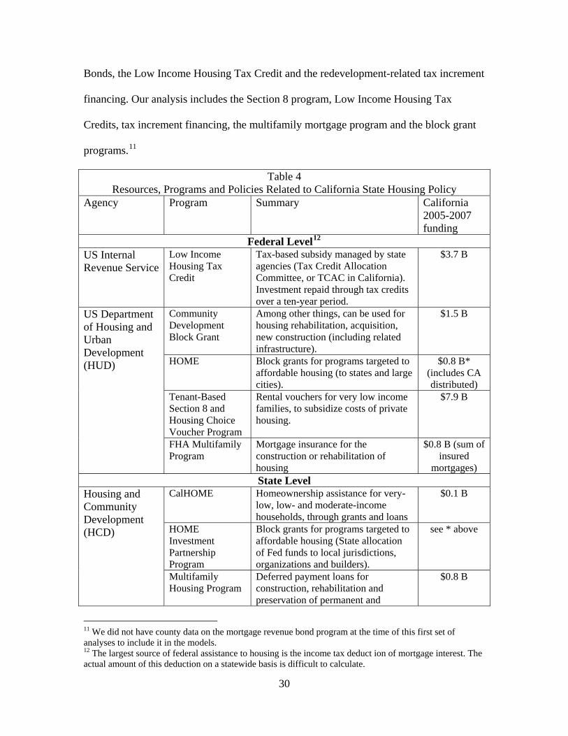
Bonds, the Low Income Housing Tax Credit and the redevelopment-related tax increment
financing. Our analysis includes the Section 8 program, Low Income Housing Tax
Credits, tax increment financing, the multifamily mortgage program and the block grant
programs.11
Table 4 Resources, Programs and Policies Related to California State Housing Policy
Agency Program Summary California 2005-2007 funding
Federal Level12
US Internal Revenue Service
Low Income Housing Tax Credit
Tax-based subsidy managed by state agencies (Tax Credit Allocation Committee, or TCAC in California). Investment repaid through tax credits over a ten-year period.
$3.7 B
Community Development Block Grant
Among other things, can be used for housing rehabilitation, acquisition, new construction (including related infrastructure).
$1.5 B
HOME Block grants for programs targeted to affordable housing (to states and large cities).
$0.8 B* (includes CA distributed)
Tenant-Based Section 8 and Housing Choice Voucher Program
Rental vouchers for very low income families, to subsidize costs of private housing.
$7.9 B
US Department of Housing and Urban Development (HUD)
FHA Multifamily Program
Mortgage insurance for the construction or rehabilitation of housing
$0.8 B (sum of insured
mortgages) State Level
CalHOME Homeownership assistance for very-low, low- and moderate-income households, through grants and loans
$0.1 B
HOME Investment Partnership Program
Block grants for programs targeted to affordable housing (State allocation of Fed funds to local jurisdictions, organizations and builders).
see * above
Housing and Community Development (HCD)
Multifamily Housing Program
Deferred payment loans for construction, rehabilitation and preservation of permanent and
$0.8 B
11 We did not have county data on the mortgage revenue bond program at the time of this first set of analyses to include it in the models. 12 The largest source of federal assistance to housing is the income tax deduct ion of mortgage interest. The actual amount of this deduction on a statewide basis is difficult to calculate.
30
Table 4 Resources, Programs and Policies Related to California State Housing Policy
Agency Program Summary California 2005-2007 funding
transitional rental housing for lower income households.
HCD and state level boards
Jobs/Housing Related Legislation
Housing and Emergency Shelter Trust Fund Acts of 2002 and 2006 (HESTFA, statewide propositions 1C and 46) provided funds for transit oriented and related housing development
$0.5 B
CalHFA Mortgage Revenue Bonds
Tax-exempt bonds issued by state and local governments to help fund below-market-interest-rate mortgages for low- to moderate-income first-time homebuyers.
$4.3 B
Local Level13
Redevelopment Agencies
Housing Set-Aside Program
Redevelopment districts are required by state law to set-aside 20 percent of their tax increment revenue for low and moderate income housing replacement and improvement.
$2.4 B
Source: Compiled by the authors from web pages and reports issued by the US Department of Housing and Urban Development, the US Internal Revenue Service, the California Department of Housing and Urban Development, and web sites explaining specific programs (full details in the References section).
Statistical Analysis Methodology
The statistical analysis uses ordinary least squares cross-sectional analysis for
California counties, of change over the time periods discussed earlier (1999 to 2005-07,
2001 to 2008, or 2001 to 2007). For each affordability indicator, we report a basic model
of economic factors expected to affect the rate of change in affordability, and a second
model including the basic variables and the policy variables. All changes are measured as
the ratio of the more recent period to the initial period.
Factors expected to change the level of affordability include:
13 There are additional funds generated at the local level, such as housing trust funds from in-lieu fees under inclusionary zoning programs and commercial linkage fees. We have not attempted to aggregate these up to the state level.
31
1. Initial conditions (price levels for homeowners and renters, the initial ratio
of labor force to employment--an indicator of the degree of commuting
required),
2. Change in the amount of housing stock
3. Changing employment conditions (employment growth, a change in
unemployment rate) and
4. Change in the labor force to employment ratio.
Several of the funding sources listed in Table 4 are included in the model on a per
capita basis. With the exception of the Section 8/Housing Choice Voucher program
(where most of the funds are allocated as vouchers in the year they are distributed), funds
included in the model are for the 2000 to 2004 period, allowing a lag between allocation
and building activity.
Because the size of counties varies widely, observations are weighted according
to county population size. Weights used are the share of the state population in the county
multiplied by the number of counties in the state (58).
Census Share of Income Affordability Measures
Table 5 gives the results for the Census based affordability measures. Each
measure is the share of income spent on housing cost (as measured by rent, homeowner
costs overall, or costs for homeowners with mortgages). Significant variables are
different for each type of indicator. Places with high median home prices in 2000 were
less likely to experience decreases in affordability for both renters and homeowners with
mortgages. For renters, denser places (more urban counties) were more likely to
experience decreases in affordability as measured by the share of income spent on rent.
32
Employment and housing construction variables in general were not significant for the
renter indicator, although places that had higher shares of labor force relative to
employment by place of work were more likely to experience decreases in affordability.
Table 5 Regression Results for Indicators Based on the Percent of Households Spending 30 Percent or More of Income on Housing Costs (Change 2000-2005-07; US Census)
Independent Variables Renters Homeowners Homeowners with Mortgage
Basic Model
With Policy Variables
Basic Model
With Policy Variables
Basic Model
With Policy Variables
Median Housing Value 2000
-5.96 E-7 (-2.15)++
-7.67 E-7 (-2.57)++
-2.09 E-7 (-0.58)
-5.27 E-7 (-1.27)
-7.38 E-7 (-2.05)++
-8.39 E-7 (-2.05)++
Median Rent 2000 2.11 E-4 (0.70)
5.23 E-4 (1.45)
-2.09 E-4 (-0.53)
1.76 E-4 (0.35)
1.61 E-4 (0.41)
2.47 E-4 (0.50)
Median Household Income (2000)
8.58 E-7 (0.24)
-2.43 E-6 (-0.62)
2.14 E-6 (0.46
-3.86 E-07 (-0.07)
5.17 E-7 (0.11)
-6.35 E-8 (-0.01)
Population Density 2.97 E-5 (3.49)+
3.08 E-5 (3.45)+
1.66 E-5 (1.49)
1.07 E-5 (0.86)
1.60 E-5 (1.47)
1.44 E-5 (1.17)
Ratio of Housing 2007 to 2000
-1.62 E-2 (-0.07)
3.27 E-1 (1.28)
3.91 E-1 (1.35)
7.40 E-1 (2.09)++
7.31 E-1 (2.59)++
1.01 (2.88)+
Ratio of unemployment rate 2007 to 2000
9.65 E-2 1.32
1.18 E-1 (1.68)
3.62 E-1 (3.80)+
3.74 E-1 (3.83)+
2.81 E-1 (3.01)+
3.10 E-1 (3.13)+
Ratio of Employment 2007 to 2000
-2.48 E-2 -0.14
-8.57 E-2 (-0.41)
-2.34 E-1 (-0.99)
-3.69 E-1 (-1.27)
-5.07 E-1 (-2.19)++
-5.83 E-1 (-2.03)++
LF to Emp ratio 2000 1.91 E-1 3.66+
2.10 E-1 (3.74)+
6.45 E-2 (0.95)
1.09 E-1 (1.40)
7.29 E-2 1.09
7.42 E-2 (0.96)
LF to Emp ratio 2007 relative to 2000
-5.76 E-2 -0.15
-1.68 E-1 (-0.40)
-2.16 E-2 (-0.04)
-3.14 E-1 (-0.55)
-6.35 E-1 (-1.28)
-7.03 E-1 (-1.24)
Per Capita Housing Assistance*
Tax Increment Fin -4.81 E-4 (-1.79)#
-5.13 E-4 (-1.39)
-2.51 E-4 (-0.68)
MF Mortgage 2.19 E-5 (0.17)
1.78 E-4 (0.59)
1.98 E-4 (0.66)
CDBG/Home 1.25 E-4 (0.51)
5.55 E-4 (1.66)
1.77 E-4 (0.53)
Section 8 funds 2000 to 2008
7.47 E-5 (2.03)++
2.74 E-5 (0.54)
5.00 E-5 (0.99)
LIHTC funds through 2004
-5.56 E-4 -(1.92)#
-3.67 E-4 (-0.92)
-5.85 E-4 (-1.48)
Constant 8.68 E-1 (1.55)
9.31 E-1 (1.54)
1.19 (1.63)
1.42 (1.69)#
2.09 (2.92)+
2.17 (2.62)++
Adj R2 (Prob > F) 0.42 (0.0000)+
0.49 (0.0000)+
0.53 (0.0000)+
0.54 (0.0000)+
0.61 (0.0000)+
0.60 (0.0000)+
33
Table 5 Regression Results for Indicators Based on the Percent of Households Spending 30 Percent or More of Income on Housing Costs (Change 2000-2005-07; US Census)
Independent Variables Renters Homeowners Homeowners with Mortgage
Basic Model
With Policy Variables
Basic Model
With Policy Variables
Basic Model
With Policy Variables
* Spending levels are for 2000 through 2004 except as otherwise specified. These dates were chosen because of the lag between when funds are allocated and when units are built or otherwise provided. T-Statistics in parentheses. Significance Levels are noted as: + 1% (the strongest results--direction of results would be other than indicated in less than 1% of cases); ++ 5%; # 10%.
Economic factors were more important for homeowner affordability. Increasing
unemployment was significantly related to decreasing affordability for all homeowners
and for those with a mortgage. In addition, increased housing stock was related to
decreasing affordability for homeowners with a mortgage (and for all homeowners in the
model including policy variables), a counter intuitive outcome, perhaps explained by the
price effects of subprime lending during the period.
In the models including policy variables, none of the policy variables were
significant for homeowners.14 For renters, both tax increment financing and low income
housing tax credits were associated with better affordability outcomes. Higher per capita
shares of Section 8 funds were associated with worsening affordability. This could be the
result of reverse causality--higher funds may go to places in greater need, and in this
case, we did not include a lag in funding because the result on ability to rent would be
immediate. There are other explanations as well. This could be a measure of the kinds of
places that received funding, or to the way the census indicator is measured--Section 8
funds would allow lower income households to pay more for housing than their income
would otherwise permit, yet may not be included in the income denominator. A further 14 Mortgage revenue bonds are a significant piece of the affordable housing policy for homeowner. The models should be rerun with data on this program.
34
complication in interpreting Section 8 funding impacts is that housing vouchers are
portable. A voucher allocated in one county could ultimately be used for a rental in a
different county (Housing Authority of Alameda County 2008).
Fair Market Rent and Salary Comparisons
Table 6 gives the results for the indicators based on HUD fair market rent (FMR)
and BLS wage data. Models are shown explaining changes for the percent of the 25th
percentile salary needed for the FMR, the percent of the median salary need for the FMR,
and the 25th percentile salary remaining after paying the FMR. These indicators were
more closely correlated than the Census indicators, and the results are consistent among
models. While not all factors significant in one model are significant in all models, the
signs of factors are entirely consistent among all significant factors (and among many
that are not statistically significant).
Table 6 Regression Results Based on Share of Wages Needed to Pay HUD Fair Market Rent
(FMR) and Remaining Salary after Paying Rent (Change over Time) Independent Variables 25 Percentile Wage
rate 2007 to 2000 (-1.30) (-1.01) (-2.07)++ (-1.80)# (2.80)+ (2.37)++ Ratio of Employment 2007 to 2000
1.71 (4.08)+
9.07 E-1 (2.11)++
1.87 (3.79)+
9.50 E-1 (1.72)#
-2.56 (-4.22)+
-1.73 (-2.54)++
LF to Emp ratio 2000 2.65 E-1 (2.20)++
2.06 E-1 (1.81)#
2.07 E-1 (1.46)
2.23 (1.52)
-3.31 E-1 (-1.90)#
-4.15 E-1 (-2.30)++
LF to Emp ratio 2007 relative to 2000
1.29 (1.45)
4.20 E-1 (0.49)
1.07 (1.02)
-1.97 E-1 (-0.18)
-2.52 (-1.95)#
-1.11 (-0.82)
Per Capita Housing Assistance*
Tax Increment Fin 7.97 E-4 (1.45)
1.60 E-4 (0.23)
2.29 E-3 (2.63)+
MF Mortgage 4.32 E-4 0.96
5.87 E-5 (0.10)
-1.00 E-3 (-1.41)
CDBG/Home 1.33 E-3 (2.71)+
1.78 E-3 (2.83)+
-1.02 E-3 (-1.32)
Section 8 funds 2000 to 2008
-1.65 E-4 (-2.19)++
-1.40 E-4 (-1.45)
5.78 E-06 (0.05)+
LIHTC funds through 2004
-1.53 E-3 (-2.60)++
-1.48 E-3 (-1.95)#
2.59 E-2 (2.78)+
Constant -1.95 (-1.50)
-2.40 E-1 (-0.19)
-1.73 (-1.14)
2.37 E-1 (0.15)
5.76 (3.07)+
3.90 (1.98)#
Adj R2 (Prob > F) 0.80 (0.0000)+
0.86 (0.0000)+
0.75 (0.0000)+
0.80 (0.0000)+
0.82 (0.0000)+
0.85 (0.0000)+
* Spending levels are for 2000 through 2004 except as otherwise specified. These dates were chosen because of the lag between when funds are allocated and when units are built or otherwise provided. T-Statistics in parentheses. Significance Levels are noted as: + 1% (the strongest results--direction of results would be other than indicated in less than 1% of cases); ++ 5%; # 10%.
For the 25th percentile and median percentile share spent on the FMR, the share
increased more where rents were initially high, and less where incomes were initially
high. Rising unemployment was significantly associated with decreasing salary shares
spend on the FMR and faster employment growth with increasing shares of income
required for the FMR (perhaps indicating that FMR was decreased where employment
36
trends were weak). For the 25th percentile households, low income housing tax credits
and section 8 funds were significantly associated with lower growth in the share of salary
spent for the FMR and with higher growth in salary remaining after paying the FMR.
Interpreting the Findings
Although not all results were as would be predicted, there was some consistency
between the two sets of models. Population density (a measure of the level of
urbanization) was positively associated with worsening affordability for both the census
renter indicator and the FMR/wage salary remainder indicator. The labor force to
employment ratio was significantly associated with worsening affordability for these two
indicators as well as for the 25th percentile share of salary indicator. Low income housing
tax credit funding had the expected effect on affordability for all three of these indicators,
as well as for the median salary share indicator. Tax increment financing was significant
in the expected direction for both the homeowners with a mortgage indicator and the
FMR/Wage salary remainder indicator.
Some of the inconsistencies and unexpected directions of significant effects can
be explained by the problem of making causal interpretations for highly aggregated data.
This also then demonstrates the limits to this type of analysis. Further analysis could
benefit from additional data (the share of mortgages in the subprime category during the
period, for example), from a more disaggregated analysis, looking at measures over
single years, or at individual household experience over time, or from in-depth case
studies of different housing and labor market areas.
37
38
On the policy side, the overlap in findings among several types of indicators for
both the low income housing tax credit and the tax increment financing funding suggest
that programs directly targeted to providing housing stock for lower or moderate income
households can improve the overall affordability for a region.
How is Funding Allocated?
A series of regressions examine the factors associated with county-wide per capita
funding levels for different funding sources (the sum for all jurisdictions). Each per capita
funding variable is measured as the 2005 to 2007 allocation of funding divided by the
2007 population level for the county. (HESFTA funding includes a small amount of pre-
2005 funding, but the large majority is for the 2005-2007 period). The models include
one institutional variable, nonprofit building capacity, measured as the ratio of the share
of California nonprofit builder assets in the county to the county’s share of California
population.15 The results are summarized in Table 7. A separate model is shown for each
of five sources of assistance: (1) Section 8 funds, (2) housing portion of tax increment
financing, (3) low income housing tax credits, (4) block grants (from both CDBG and
HOME sources), and (5) HESTFA programs. Significant factors vary among the different
funding sources, but most differences are consistent with the purpose of the specific
program. The signs are consistent among models for most of the significant variables,
with only two exceptions.
15 Data on nonprofit builder assets came from National Center for Charitable Statistics 2009 and was for the year 2001. We also developed a measure of inclusionary ordinance coverage (share of residential permit activity in the county covered by places with inclusionary ordinances) which was not significant in any of our preliminary models, and is not included in the models shown.
39
Table 7 Regressions Testing the Factors Influencing Recent Allocations from Selected Funding Sources
Independent Variables Dependent Variables--Program Per Capita Allocation, 2005-07 (1)
Section 8 (2)
Housing Share, Tax Increment Financing
(3) Low Income Housing Tax
Credit
(4) CDBG
and Home
(5) Housing and Emergency
Shelter Trust Fund Act
(6) Total Housing
Subsidies
Per capita income 2000 -8.01 E-3 (-2.36)++
-1.87 (-1.56)
3.27 E-3 (-0.90)
1.59 E-3 (1.92)#
-2.04 E-3 (-1.18)
-4.91 E-3 (-1.06)
Median home value 2000 1.12 E-3 (2.74)+
-1.20 E-4 (-0.78)
-3.62 E-4 (-0.83)
-1.51 E-4 (-1.43)
1.87 E-5 (0.08)
2.41 E-4 (0.41)
Median rent 2000 -9.20 E-1 (-4.50)+
2.26 E-1 (3.62)+
-5.08 E-1 (-2.32)++
-7.26 E-2 (-1.68)#
-2.10 E-1 (-2.33)++
-5.61 E-1 (-2.33)
Percent homeowners with 30%+ cost share
NA 208.80 (1.57)
NA 500.6 (5.42)+
234.90 (1.22)
151.9 (0.29)
Percent of 25th percentile salary for FMR
3425.3 (6.63)+
41.41 (0.27)
1259.8 (2.27)++
72.73 (0.68)
951.42 (4.25)+
2183.86 (3.65)+
Residual 25th percentile salary remaining after paying FMR
1.49 (6.24)+
7.30 E-2 (1.02)
5.10 E-1 (2.00)#
5.46 E-2 (1.10)
5.17 E-1 (5.02)+
1.11 (4.03)+
Population density -2.94 E-2 (-2.53)++
-2.97 E-3 (-0.70)
-4.18 E-2 (-3.36)+
1.72 E-3 (0.58)
-7.20 E-3 (-1.17)
-2.04 E-2 (-1.24)
Labor force/ employment ratio
-109.83 (-1.66)
50.36 (2.27)++
-188.35 (-2.66)+
-69.20 (-4.50)+
-119.20 (-3.72)+
-231.56 (-2.70)+
Nonprofit housing builder capacity
-6.55 (-0.53)
13.56 (3.56)+
16.39 (1.25)
7.03 (2.66)++
7.84 (1.43)
38.28 (2.60)++
Constant -1796.96 (-5.58)+
-245.84 (-2.37)
-323.35 (-0.94)
-73.59 (1.02)
-485.19 (-3.24)+
-911.62 (-2.27)
Adj R2 (Prob > F) 0.71 (0.0000)+ 0.37 (0.0002)+ 0.23 (0.0064)+ 0.70 (0.0000)+ 0.51 (0.0000)+ 0.48 (0.0000)+ NA: Homeowner affordability measure excluded for programs relevant only to renter housing. Cells show coefficient with t-statistic in parentheses; Significant in bold: + 1%; ++ 5%; # 10%
Section 8 Funding
Section 8 funding was higher for places with low per capita incomes, higher
median home values, and lower median rents. Higher levels of Section 8 funding went to
places with higher percent of salary spent for the FMR but also with higher residual
incomes after paying FMR. This suggests the funding, while going to lower income
places with higher housing costs, may not be hitting those places where renters are most
in need after paying rent. Section 8 funding was also significantly higher in less dense
places, perhaps explaining why the residual salary remainder variable was positively
associated with per capita funding. The lowest residual rents were in urban places, while
some of the highest residuals were in the smaller, less urban counties.16
Tax Increment Financing
The tax increment financing variable was not as well explained by many of the
indicators of affordable housing need. Although we include no overall measure of
presence of redevelopment districts, the model illustrates the different mix of factors
driving this funding. Places with higher median rents, and higher ratios of labor force to
employment tended to have higher levels of tax increment financing per capita. Tax
increment financing was also positively and significantly related to nonprofit builder
capacity. The nonprofit builder capacity may be an indicator in this case of the overall
county capacity for developing the private public partnerships necessary for
redevelopment activities.
Low Income Housing Tax Credits
16 The portability problem discussed in an earlier footnote is also relevant to the results for this model.
40
The low income housing credit allocation model had relatively weak explanatory
power, but several interesting variables were significant. Places with lower rents in 2000,
but where low income renters paid high shares of salary for rents were more likely to
received tax credit allocations. The residual rent measure was weakly positively
significant, and the density measure negative and significant, suggesting a funding
distribution somewhat similar to the section 8 distribution. The funding was more likely
to go to places where the labor force to employment ratio was lower (indicating a focus
on the need to accommodate more workforce housing).
CDBG and HOME Funding
The model explained much of the block grant funding distribution, and indicated
that a number of factors independent of housing need influence the distribution of this
funding. Per capita funding overall is positively related to income level and negatively
related to median rents. The only significant housing need variable was the percent of
homeowners paying more than 30 percent of income on homeowner costs. Workforce
housing needs also appear to be taken into account, as funding is higher where the labor-
force to employment ratios are lower. Nonprofit housing capacity also was significant
and positively associated with funding levels.
Housing and Emergency Shelter Trust Fund Act
Housing and Emergency Shelter Trust Fund Act funding (also known as
Proposition 46 and 1C funding) addresses both affordability and jobs/housing balance
issues. The funding is positively correlated with places with lower rents and higher shares
of salaries needed for the FMR. It is negatively related to the labor force-employment
ratio. As with the Section 8 funds, the salary remainder variable is positively related to
41
the funding, again indicating that there is some discrepancy among the results for the
affordability variables.
Total Housing Subsidies
Combining all housing subsidies gives a picture of the kinds of places that are
receiving affordable housing assistance. It is appropriately going to places with higher
rents relative to wages, and lower labor force to employment ratios. Among these places,
it is being spent where rents were relatively low. This may occur because affordable
housing is not accepted or not feasible in the highest priced areas. The residual salary
measure continues to be significant in the opposite direction from the other affordability
measures, suggesting that further attention might be needed to the balance between cost
and ability to pay. The importance of nonprofit capacity is confirmed by the analysis of
combined funding levels.
Case Examples: Marysville, Riverside and Santa Barbara
Experiences at the local level underline some of the findings indicated by the
statistical models and suggest other considerations not addressed in the preceding
discussions. We selected three California cities to use as case examples of affordable
housing levels, strategies, and funding, including Marysville (Yuba County), Riverside
(Riverside County), and Santa Barbara (Santa Barbara County). These places were
selected based on their counties’ affordability (measured as the percentage of median
wage needed to afford Fair Market Rent in 2008) relative to the per capita affordable
housing support received over a three-year period (2005-2007) from tax increment
financing, low income tax credits, block grants and the range of programs through the
42
Emergency Housing and Shelter Trust Fund Acts. Among California’s counties, Yuba
(where Marysville is located) had the fourth highest funding per capita, and was one of
the most affordable places to live. Riverside and Santa Barbara were both highly
unaffordable, with the former receiving a high share of funds, and the latter a low share,
as measured on a per capita basis.
Background on Affordability
Each city, with its varying degree of affordability, faces unique challenges.
Marysville, though relatively more affordable, is largely populated by low-income
households whose average income is below the poverty level. Riverside is experiencing
an increasing demand for housing, due to population growth and workers in coastal cities
looking for more affordable housing inland. Santa Barbara, like many of California’s
cities, struggles with high housing costs and low vacancy rates, as well as a lack of
housing suited to its working population. In all three places, renters paid a higher share of
income than homeowners in both 2000 and 2007. Marysville, Riverside, and Santa
Barbara each experienced a significant increase from 2000 to 2007 in the percentage of
all households whose housing costs exceeded 30 percent of income.
Table 8 Comparative Population and Housing Data for Case Example Cities
Sources: California Department of Finance Table E-5a; interviews.
43
Affordable Housing Efforts
Affordable housing projects are a significant share of new homes added--ranging
from just under one fourth in Riverside to eighty percent in Santa Barbara. (See Table 8.)
Each of the three cities has used a mixture of funds to address housing needs for low and
moderate income households, including CDBG, HOME, FHA’s multifamily insured
mortgages, state propositions, tax increment financing districts, Housing Choice
Vouchers, and Low Income Housing Tax Credits. For all three cities, tax credits played a
significant role in providing resources for the building of affordable units. From 2005
through 2007, Marysville received over $24 million in tax credits, while Riverside and
Santa Barbara each received over $11 million. City or county affiliated organizations,
nonprofit agencies, and private builders have all contributed to building activity, but at
different levels in each city.
Marysville's experience points to the limits of the affordability indicators used to
assess aggregate county trends. The city has had little in the way of net additions to
housing stock in the 2000 to 2007 period, but affordable projects were a substantial part
of new building. The California Department of Finance estimates only a 17 unit increase
in housing stock in Marysville, but city records show 23 affordable units during the
period, of which 11 were single family homes and 23 were rental units in a rehabilitated
downtown building. The Yuba County Office of Education’s organization Youth Build
was responsible for building the single-family homes, while the local redevelopment
agency allocated HUD funds for the 12 converted rental units. In addition, over the 2000
to 2007 period, the city received Low Income Housing Tax Credits for the rehabilitation
of 143 units. The importance of rehabilitated units in the affordable housing strategy
44
suggests that even though the indicators look relatively strong, quality of housing may be
an issue in the city and county.
The role of several different types of players and a wide range of resources stands
out in Riverside's experience adding affordable units. More than one third of all
affordable units built over the eight year period relied on some level of tax credit
financing. The redevelopment agency’s tax increment financing district, in place since
1976, was the second largest contributor to affordable housing projects. No single
developer stands out as dominating the local market, but rather a combination of
organizations – including the Riverside Housing Development Corporation, various
nonprofits, and LLCs - has driven the production of affordable units. Some projects
combined several sources of funds in producing units. For example, the nonprofit
National CORE built Mission Pointe in Riverside, which offered 2- and 3-bedroom units
for very low- and low-income family households. The project was completed using
funds from the redevelopment agency, HOME, and tax credits. The majority of the city’s
funds are currently being used to purchase and rehabilitate foreclosed houses to be sold to
first-time homebuyers, according to Michelle Davis, the city's housing coordinator (Davis
2009).
In Santa Barbara, the combination of tax credits and nonprofit builders has been
critical to the provision of affordable units, according to Steven Faulstich, Housing
Programs Supervisor (Faulstich 2009). The Housing Authority has made significant
contributions to Santa Barbara’s affordable housing stock since 2000, creating more than
1/4 of the new units. Nonprofit organizations have also been a critical presence in the
city, particularly Peoples’ Self-Help Housing (PSHH) and Habitat for Humanity of
45
Southern Santa Barbara County. In 2004, PSHH built Casas las Granadas, a 12-unit
rental development for low-income households. The project received over $1 million
each from HUD’s HOME funds and LIHTC, and an additional $60,000 came from state
funding. Tax credits also helped finance a variety of other new construction projects
between 2000 and 2007, including Mercy Housing’s 75-unit development for large
family households.
Other Approaches to Maintaining Affordability and Access
Both Riverside and Santa Barbara rely on additional strategies to deal with the
pressures on housing brought about by employment pressures and other types of demand.
In contrast, Marysville, surrounded by levees and almost entirely built out, has fewer
options for influencing private sector housing development; the jobs/housing balance can
be seen as more of a county issue where there is more room for new construction (Lamon
2009).
Riverside has attempted to address the issue by providing higher density bonuses
in housing developments located near transit stations and corridors. Santa Barbara has
seen job pressures as part of the issue in providing affordable housing. The city has
15,000 incoming commuters every day coming in for the jobs, but priced out of local
housing. Nearly 30 years ago, voters decided to set strict limits on the square footage of
new commercial development within the city, hoping to lessen the jobs/housing
imbalance. However, the density of employees per building has increased (with
modulation), and the square footage limit has not limited the number of employees and
has not rectified the jobs-housing balance.
46
Santa Barbara is the only case example city that has an inclusionary housing
ordinance (as does Santa Barbara County). The inclusionary requirements are designed
to increase the stock of for-sale, ‘middle’ income homes (120-160% AMI). Because
there are so few tracts of land large enough for developments (of 10 units or more) that
would require an inclusionary component, only 2 projects in the past four years have
qualified.
Implications
These case snapshots underline several points. First, while summary data by
county gives a useful overview of trends and conditions, local experience is equally
important in understanding circumstances and creating policy. Second, additional
indicators may be needed to provide a more complete picture of affordability, including
measures of persons per room and housing quality. Third, changing economic conditions
require changing strategies. Riverside's focus on incorporating foreclosed properties into
their current approach to developing affordable housing stock is a response not only to
new supply but to new financing conditions for the provision of affordable and for-
market units. Fourth, the city experiences emphasize the importance of local, state, and
federal funding sources in supporting investment in affordable housing. At least two of
the three cities (Marysville and Santa Barbara) likely would have had no affordable
housing development without these funds, given the amount of new housing added in
Marysville in the period, and the cost of land in Santa Barbara. For Riverside, what was
once affordable housing was quickly becoming less affordable with the added pressure of
job growth from outside and within the county; units that are built under restrictions that
leave them affordable help to maintain the base in these circumstances.
47
Conclusions
In interpreting affordability indicators, it is important to keep in mind what the
indicators measure. The share of income spent means little unless the context is
understood--what is the base income level, how does this compare to other locations, how
has the base, as well as the share, changed over time. Furthermore, cost relative to
income does not tell the full story. The density of occupancy (persons per household) and
quality of units are also significant indicators of affordability. More than one type of
indicator may be needed to understand whether housing affordability is improving or
worsening, and to identify differences among places.
The affordability indicators used in this analysis show that overall, the share of
income spent on housing costs increased between 2000 and 2007, but that these changes
are sensitive to the time increments chosen and to economic events during the period.
The San Francisco Bay Area, for example, faced peak rental costs as a result of the dot-
com boom in 2000, so an improvement in the share of income spent on rent is not
surprising over the subsequent seven years. The residual income indicator is an important
modifier to the share of income indicator, confirming that several San Francisco Bay
Area counties showed strength not only relative to the previous costly period but also in
comparison to other places in the state. In contrast, multiple indicators show worsening
housing affordability in Los Angeles County and several other large southern California
counties.
The statistical analysis as well as examples of three California cities show the role
played by federal, state and local affordable housing programs in improving affordability.
48
Both the low income housing tax credit and tax increment financing were significantly
related to improvements in affordability for more than one indicator, while other funding
sources did not show this direct link to improvement in affordability. The different
funding sources are distributed according to somewhat varying sets of needs, but in
general have gone to places where either homeowners or renters are paying high shares of
income for housing costs. Some sets of funds also showed allocation based on
jobs/housing balance needs. In addition, the strength of nonprofit capacity, as measured
by employment in nonprofit builders as a share of total employment in the county, was
directly associated with higher per capita levels of tax increment and block grant funding,
and with total per-capita funding levels. The record of what is built in the cities we
examined confirmed the role of nonprofit builders in providing affordable housing. The
for-profit development sector continues to play a role, but it is a complex one that
involves juggling requirements and incentives and is very sensitive to economic
conditions.
Some important caveats should be taken into account in using these results. First,
the statistical analysis was done almost entirely at the county level. Additional
information could be gained from bringing in information from the local jurisdictional
level, from conducting some analysis at the household level, and from much more
detailed case analysis. Second, the time period used, 2000 through 2007, is during a
period of overall growth in the economy and in building activity. Much of the funding
available for affordable housing may be less effective in an economic downturn. For
example, tax credits are a useful incentive only when the builder has income against
which to use the credits. Because affordability will remain a concern for some segments
49
of the population, even with a slowing economy (in some cases because of a slowing
economy), alternative strategies may be needed to maintain and expand the stock of
affordable units during this period. At the some time, the economic downturn may itself
address some of the affordability problem by lowering costs, at least for those households
that continue to have employed workers, by reducing home prices and rents. Even this
may be only half the story, as tightening credit and existing credit problems may make it
difficult for a larger segment of the population to take advantage of lower costs.
50
References
Bair, Sheila C. 2008. "A Review of Foreclosure Mitigation Efforts." Statement before the Financial Services Committee U.S. House of Representatives. Washington D.C., September 17, 2008. http://www.fdic.gov/news/news/speeches/chairman/spsep1708.html
California Association of Realtors. 2008a. Annual Historic Data Summary 2008.
California Association of Realtors: Los Angeles. Page 23. _______________. 2008b. "First-time Buyer Housing Affordability Index
Methodology." Web Page. http://www.car.org/economics/marketdata/ftbhaimethodology/. Accessed December 19, 2008.
California Budget Project. 2004. Locked Out 2004: California’s Affordable Housing
Crisis. http://www.cbp.org/pdfs/2004/lockedout2004.pdf (accessed January 2008).
Davis, Michelle. 2009. Housing Coordinator, Riverside. Personal Interview (e-mail).
January 12, 2009. Faulstich, Steven. 2009. Housing Program Supervisor, Santa Barbara. Personal Interview
(telephone). January 12, 2009 Hancock, K.E. 1993. "'Can Pay? Won't Pay? or Economic Principles of 'Affordability.'"
Urban Studies. 30 (1): 127-145. Housing Authority of Alameda County. 2008. Portability. Web Site: http://www.haca.net/index.php?option=com_content&view=article&id=73&Itemid=69 Last updated November 24; Accessed January 29, 2009. Hulchanski, J. David. 1995. "The Concept of Housing Affordability: Six Contemporary
Uses of the Housing Expenditure-to-Income Ratio." Housing Studies. 10 (4):471-491. October.
Kutty, Nandinee K. 2005. "A New Measure of Housing Affordability: Estimates and
Analytic Results." Housing Policy Debate. 16 (1): 113-142. Lamon, David. 2009. City Services Director, Marysville. Personal Interview (e-mail).
January 20, 2009. Lowry, Ira S., Carol E. Hillestad, and Syam Sarma. 1983. California's Housing:
Adequacy, Availability, and Affordability. Rand: Santa Monica. October.
51
National Association of Home Builders. 2008. "What is the NAHB-Wells Fargo Housing Opportunity Index (HOI)?" Web Page. http://www.nahb.org/generic.aspx?sectionid=135&genericcontentid=533. Last accessed December 15, 2008.
National Association of Realtors. 2008. "Methodology for the Housing Affordability
Index." Web Page. http://www.realtor.org/research/research/hameth. Accessed December 19, 2008.
National Center for Charitable Statistics. 2009. NCCS All Registered Nonprofits Table
Wizard. http://nccsdataweb.urban.org/tablewiz/tw_bmf.php. Accessed September 8, 2009.
Rosen, Kenneth T. 1984. California Housing Markets in the 1980s: Demand,