2 I. Physikalisches Institut, Universität zu Köln, Zülpicher Straße 77, 50937 Köln, Germanye-mail: [email protected]
3 Max-Planck-Institut für Extraterrestrische Physik, Giessenbachstrasse 1, 85748 Garching, Germany4 Department of Astrophysics, American Museum of Natural History, 79th St. at Central Park West, New York, NY 10024, USA
e-mail: [email protected] Zentrum für Astronomie, Institut für Theoretische Astrophysik, Universität Heidelberg, Albert-Ueberle-Str. 2,
69120 Heidelberg, Germany6 Center for Computational Astrophysics, Flatiron Institute, 162 Fifth Ave, New York, NY 10010, USA
Received 27 July 2018 / Accepted 9 August 2019
ABSTRACT
Context. Supersonic disordered flows accompany the formation and evolution of molecular clouds (MCs). It has been argued that thisis turbulence that can support against gravitational collapse and form hierarchical sub-structures.Aims. We examine the time evolution of simulated MCs to investigate: What physical process dominates the driving of turbulentflows? How can these flows be characterised? Are they consistent with uniform turbulence or gravitational collapse? Do the simulatedflows agree with observations?Methods. We analysed three MCs that have formed self-consistently within kiloparsec-scale numerical simulations of the interstellarmedium (ISM). The simulated ISM evolves under the influence of physical processes including self-gravity, stratification, magneticfields, supernova-driven turbulence, and radiative heating and cooling. We characterise the flows using velocity structure functions(VSFs) with and without density weighting or a density cutoff, and computed in one or three dimensions. However, we do not includeoptical depth effects that can hide motions in the densest gas, limiting comparison of our results with observations.Results. In regions with sufficient resolution, the density-weighted VSFs initially appear to follow the expectations for uniformturbulence, with a first-order power-law exponent consistent with Larson’s size-velocity relationship. Supernova blast wave impactson MCs produce short-lived coherent motions at large scales, increasing the scaling exponents for a crossing time. Gravitationalcontraction drives small-scale motions, producing scaling coefficients that drop or even turn negative as small scales become dominant.Removing the density weighting eliminates this effect as it emphasises the diffuse ISM.Conclusions. We conclude that two different effects coincidentally reproduce Larson’s size velocity relationship. Initially, uniformturbulence dominates, so the energy cascade produces VSFs that are consistent with Larson’s relationship. Later, contraction dominatesand the density-weighted VSFs become much shallower or even inverted, but the relationship of the global average velocity dispersionof the MCs to their radius follows Larson’s relationship, reflecting virial equilibrium or free-fall collapse. The injection of energy byshocks is visible in the VSFs, but decays within a crossing time.
It has long been known that star formation preferentially occurswithin molecular clouds (MCs). However, the physics of thestar formation process is still not completely understood. It isobvious that gravity is the key factor for star formation as itdrives collapse motions and operates on all scales. However, oneneeds additional processes that stabilise the gas or terminate starformation quickly in order to explain the low star formation effi-ciencies observed in MCs. Although there are many processesthat act at the different scales of MCs, turbulent support has oftenbeen argued to be the best candidate for this task.
In the literature, turbulence plays an ambiguous role in thecontext of star formation. In most of the cases, turbulence isexpected to stabilise MCs on large scales (Fleck 1980; McKee &Zweibel 1992; Mac Low 2003), while feedback processes andshear motions heavily destabilise or even disrupt cloud-likestructures (Tan et al. 2013; Miyamoto et al. 2014). However, it
remains unclear whether there are particular mechanisms thatdominate the driving of turbulence within MCs, as every processis supposed to be traced by typical features in the observables.Yet, these features are either not seen or are too ambiguous toclearly reflect the dominant driving mode. For example, turbu-lence that is driven by large-scale velocity dispersions duringglobal collapse (Ballesteros-Paredes et al. 2011a,b; Hartmannet al. 2012) produces P-Cygni line profiles that have not yetbeen observed on scales of entire MCs. Internal feedback, onthe contrary, seems more promising as it drives turbulence fromsmall to large scales (Dekel & Krumholz 2013; Krumholz et al.2014). Observations, though, demonstrate that the required driv-ing sources need to act on scales of entire clouds, which typicalfeedback, such as radiation, winds, jets, or supernovae (SNe),cannot achieve (Heyer & Brunt 2004; Brunt et al. 2009; Brunt &Heyer 2013).
There have been many theoretical studies that have examinedthe nature and origin of turbulence within the various phases of
A97, page 1 of 21Open Access article, published by EDP Sciences, under the terms of the Creative Commons Attribution License (http://creativecommons.org/licenses/by/4.0),
which permits unrestricted use, distribution, and reproduction in any medium, provided the original work is properly cited.Open Access funding provided by Max Planck Society.
the interstellar medium (ISM; Mac Low & Klessen 2004, andreferences within). The most established characterisation of tur-bulence in general was introduced by Kolmogorov (1941) whoinvestigated fully developed, incompressible turbulence drivenon scales larger than the object of interest, and dissipating onscales much smaller than those of interest. In the scope of thispaper this object is a single MC. MCs are highly compress-ible, though. Only a few analytical studies have treated thiscase. She & Lévêque (1994) and Boldyrev (2002), for example,generalised and extended the predicted scaling of the decay ofturbulence to supersonic turbulence. Galtier & Banerjee (2011)and Banerjee & Galtier (2013) provided an analytic descriptionof the scaling of mass-weighted structure functions.
Larson (1981) found a relation between the linewidth σ andthe effective radius R of MCs. Subsequent investigators havesettled on the form of the relation being (Solomon et al. 1987;Falgarone et al. 2009; Heyer et al. 2009)
σ ∝ R1/2. (1)
Goodman et al. (1998) showed that analysis techniques usedto study this relation could be distinguished by whether theystudied single or multiple clouds using single or multiple tracerspecies. Explanations for this relation have relied on eitherturbulent cascades (Larson 1981; Kritsuk et al. 2013a, 2015;Gnedin 2015; Padoan et al. 2016), or the action of self-gravity(Elmegreen 1993, 2007; Vázquez-Semadeni et al. 2006; Heyeret al. 2009; Ballesteros-Paredes et al. 2011b).
These can potentially be distinguished by examining thevelocity structure function (VSF). Kritsuk et al. (2013a) care-fully reviews the argument for Larson’s size-velocity relationdepending on the turbulent cascade. In short, in an energy cas-cade typical for turbulence, the second-order structure functionhas a lag dependence `ζ(2) with ζ(2)' 1/2. In Ibáñez-Mejíaet al. (2016, hereafter Paper I) the authors argue that uniformdriven turbulence was unable to explain the observed relationin a heterogeneous ISM, but that the relation could be naturallyexplained by hierarchical gravitational collapse.
In this paper, we examine the velocity structure functionsof three MCs that formed self-consistently from SN-driven tur-bulence in the simulations by Paper I and Ibáñez-Mejía et al.(2017, hereafter Paper II). We study how the turbulence withinthe clouds’ gas evolves. The key questions we address are thefollowing: What dominates the turbulence within the simulatedMCs? Does the observed linewidth-size relation arise from theturbulent flow? How can structure functions inform us aboutthe evolutionary state of MCs and the relative importance oflarge-scale turbulence, discrete blast waves, and gravitationalcollapse?
In Sect. 2, we introduce the simulated clouds in the context ofthe underlying physics involved in the simulations. Furthermore,we describe the theoretical basics of velocity structure functions.Section 3 demonstrates that the velocity structure function isa useful tool to characterise the dominant driving mechanismsof turbulence in MCs and can be applied to both simulatedand observed data. We examine the influence of using one-dimensional velocity measurements, different Jeans refinementlevels, density thresholds, density weighting on the applicabilityof the velocity structure function, and the results obtained withit in Sect. 4. At the end of that section, we also compare ourresults to observational studies. We summarise our findings andconclusions in Sect. 5. The simulation data and the scripts thatthis work is based on are published in the Digital Repository ofthe American Museum of Natural History (Chira et al. 2018a).
2. Methods
2.1. Cloud models
The analysis in this paper is based on a sample of three MCsidentified within a three-dimensional (3D), magnetohydrody-namical, adaptive mesh refinement simulation using the FLASHcode (Fryxell et al. 2000). Paper I and Paper II, as well asChira et al. (2018b, Paper III hereafter), describe the simulationsand the clouds in more detail. We summarise the most relevantproperties.
The numerical simulation models a 1× 1× 40 kpc3 sectionof the multi-phase, turbulent ISM of a disc galaxy, where densestructures form self-consistently in convergent, turbulent flowsPaper I. The model includes gravity – a background galactic-discpotential accounting for a stellar component and a dark matterhalo, as well as self-gravity turned on after 250 Myr of simulatedtime – SN-driven turbulence, photoelectric heating and radiativecooling, and magnetic fields. Although hundreds of dense cloudsform within the simulated volume, Paper II focussed on threeclouds, which were re-simulated at a much higher spatial res-olution. The internal structures of the MCs are resolved usingadaptive mesh refinement, focussing grid resolution on denseregions where Jeans unstable structures must be resolved witha minimum of 4 cells (λJ > 4∆xmin). For a maximum resolutionof ∆x = 0.1 pc, the corresponding maximum resolved density is8× 103 cm−3 for gas at a temperature of 10 K (e.g. Paper II,Eq. (15)). We define MCs as regions above a fixed number den-sity threshold with fiducial value ncloud = 100 cm−3. We chosethis threshold as it roughly corresponds to the density when CObecomes detectable. The MCs have initial masses at the onset ofself-gravity of 3× 10³, 4× 10³, and 8× 10³ M� and are denotedas M3, M4, and M8, respectively, hereafter. In this paper, we use thedata within (40 pc)3 subregions centred on the high-resolutionclouds’ centres of mass, which we map to a uniform grid of 0.1pc zones for analysis. For illustrations of the morphologies of thethree clouds we refer to Fig. 1 of Paper III.
It is important to point out that the clouds are embeddedwithin a complex turbulent environment, gaining and losingmass as they evolve. Paper II described the time evolution ofthe properties of all three clouds in detail, in particular, mass,size, velocity dispersion, and accretion rates, in the contextof MC formation and evolution within a galactic environment.Paper III studied the properties, evolution, and fragmentationof filaments that self-consistently condense within these clouds.We paid particular attention to the accuracy of typical stabil-ity criteria for filaments, comparing the results to the theoreticalpredictions, showing that simplified analytic models do not cap-ture the complexity of fragmentation due to their simplifyingassumptions.
2.2. Velocity structure function
In this paper, we probe the power distribution of turbulencethroughout the entire simulated MCs by using the velocitystructure function (VSF). The VSF is a two-point correlationfunction,
S p(`) = 〈 |∆u|p 〉 (2)
that measures the mean velocity difference
∆u(`) = u(x + `) − u(x) (3)
between two points x and x + `, with ` being the directionvector pointing from the first to the second point. The VSF S p is
A97, page 2 of 21
R.-A. Chira et al.: How do velocity structure functions trace gas dynamics in simulated molecular clouds?
usually reported as a function of lag distance, `= |`|, between thecorrelated points. The coherent velocity differences measured bythe VSF can be produced by both the energy cascade expectedin turbulent flows, and by coherent motions such as collapse,rotation, or blast waves. Those patterns become more prominentthe higher the value of the power p is (Heyer & Brunt 2004).
For fully developed, homogeneous, isotropic, turbulence theVSF is well-described by a power-law relation (Kolmogorov1941; She & Lévêque 1994; Boldyrev 2002):
Sp(`) ∝ `ζ(p). (4)
Kolmogorov (1941) predicts that the third-order exponent,ζ(3), is equal to unity for an incompressible flow. As a conse-quence the kinetic energy decays with Ekin(k)∝ k−
53 , with k = 2π
`being the wavenumber of the turbulence mode. For a supersonicflow, however, ζ(3)> 1 is expected. Based on Kolmogorov’swork, She & Lévêque (1994) and Boldyrev (2002) extended andgeneralised the analysis and predicted the following intermit-tency corrections to Kolmogorov’s scaling law. For incompress-ible turbulence with filamentary dissipative structures She &Lévêque (1994) predict that the VSFs scale with power lawindex
ζ(p) =p9
+ 2
1 − (23
) p3 , (5)
while supersonic flows with sheet-like dissipative structures arepredicted to scale with (Boldyrev 2002)
ζ(p) =p9
+ 1 −(
13
) p3
. (6)
It should be noted that both equations return a value ofζ(3) = 1, but this is only an exact result for the She & Lévêquemodel, while it is a result of normalisation in the case ofBoldyrev.
In the case of compressible turbulence, the energy cascadecan no longer be expressed in terms of a pure velocity differ-ence because density fluctuations become important. Turbulenceshould then show a cascade in some density-weighted VSF anal-ogous to the incompressible case. Padoan et al. (2016) defined adensity-weighted VSF to attempt to capture this process, whichwe use in our subsequent analysis
Alternatives have been proposed by Kritsuk et al. (2013b)based on an analysis of the equations of compressible flow thatshould be explored in future work.
In many cases a three-dimensional computation of the VSFcannot be performed because of the observational constraint thatonly line-of-sight velocities are available. We therefore compareour three-dimensional (3D) results to one-dimensional (1D),density-weighted VSFs
with ei representing the unit vector along the i = x-, y-, or z-axis.Benzi et al. (1993) introduced the principle of extended
self-similarity. It proposes that there is a constant relationshipbetween the scaling exponents of different orders at all lag scales
so that ζ can be measured from S p/S 3, which typically givesa clearer power-law behaviour. The self-similarity parameter isdefined as
Z(p) =ζ(p)ζ(3)
. (9)
As mentioned before, both Eqs. (5) and (6) return valuesof ζ(3) = 1. Therefore, those equations also offer predictions forZ(p).
For the discussion below, we measure ζ(p) by fitting a power-law, given by
log10
[S p(`)
]= log10 (A) + ζ(p) log10(`), (10)
with A being the proportionality factor of the power-law to thesimulated measurements. We choose the smallest lag of the fit-ting range to be equal to eight zones, sufficiently large to ensurethat our fit does not include the numerical dissipation range. Formore details of the fitting procedure we refer to Appendix A.
We follow observational practice and reduce the compu-tational effort of this study by generally focussing on cloudsdefined by a density threshold. However, Paper II shows thatthere is usually no sharp increase in density between the ISMand the clouds. Instead, the gas becomes continuously densertowards the centres of mass within the clouds. Consequently,our use of a density threshold is a somewhat artificial bound-ary between the clouds and the ISM. Observationally, however,introducing a column density (or intensity) threshold is unavoid-able, be it due to technical limitations (e.g. detector sensitivity)or the nature of the underlying physical processes (for example,excitation rates, or critical densities). Therefore, we also studyhow a density threshold influences the VSF and its evolution.
At our fiducial density threshold, we actually consider only≤1.5% of the volume in the high resolution cube. To under-stand the influence of this limitation we set up a test sce-nario (see Sect. 3.4) by removing the density threshold (settingncloud = 0 cm−3) that results in analysing the entire data cube.Details of the method for computing the VSFs in these two casesare given in Appendix A.
As in the case without a density threshold it would be toocomputationally expensive to compute all lags to all zones.Thus, we randomly choose a set of 5% of the total number ofzones as reference points and only compute relative velocitiesfrom the entire cube to these zones. By choosing the start-ing points randomly we ensure that all parts of the cubes areconsidered. As a consequence, there is only a small likelihood(5%× 1.5% = 0.075%) that any given zone chosen will be withinthe cloud. Therefore, we emphasise that it is likely that the twosubsamples (no density threshold and cloud-only) do not havea common subset of starting vectors. Nevertheless, the randomsample still includes >4× 10³ zones in the cloud, so the sampledoes include information on VSFs of material in the cloud.
3. Results
3.1. Examples
In this section, we present our results on how VSFs reflect thevelocity structure within and around MCs.
Figure 1 shows nine examples of density-weighted VSFs(Eq. (7)). The figure shows the VSFs of all three clouds(columns) at times of 1.0, 3.0, and 4.2 Myr after the onset ofgravity. All plots show orders p = 1–3. The solid lines show thefitted power-law relations as given by Eq. (10).
A97, page 3 of 21
A&A 630, A97 (2019)
10 1
100
101
S()
[(km
s1 )
p ]
t = 1.0 MyrM3
p = 1p = 2p = 3
t = 1.0 MyrM4
t = 1.0 MyrM8
10 1
100
101
S()
[(km
s1 )
p ]
t = 3.0 Myr t = 3.0 Myr t = 3.0 Myr
100 101
[pc]
10 1
100
101
S()
[(km
s1 )
p ]
t = 4.2 Myr
100 101
[pc]
t = 4.2 Myr
100 101
[pc]
t = 4.2 Myr
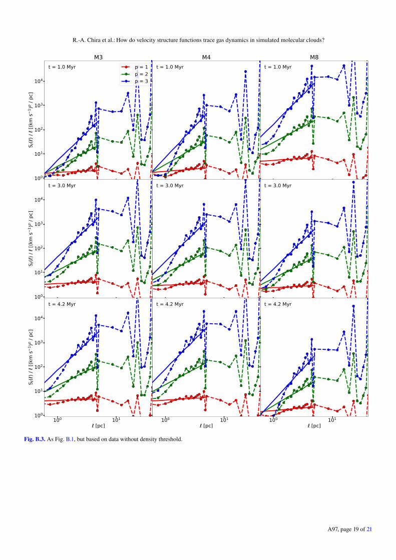
Fig. 1. Examples of VSFs from models (left to right) M3, M4, and M8 as function of lag scale ` and order p, based on data with density threshold.The examples are given for times (top to bottom) t = 1.0 Myr, 3.0 Myr, and 4.2 Myr. The dots (connected by dashed lines) show the values computedfrom the simulations. The solid lines represent the power-law relation fitted to the respective structure functions.
The examples demonstrate that, in general, the measuredVSFs cannot be described by a single power-law relation overthe entire range of `. Instead they are composed of roughly threedifferent regimes: one at small scales at 0.8 pc. `. 3 pc, a sec-ond one within 3 pc. `. 10–15 pc, and the last one at largescales with 10–15 pc. `. 30 pc. We find that only the small andintermediate ranges may be represented by a common power-law
relation. On larger scales, one observes a local minimum beforethe VSFs either increase or stagnate. Additional examples ofVSFs are given in Appendix B.
The examples in Fig. 1 and Appendix B illustrate how VSFsreact to different scenarios that affect the turbulent structure ofthe entire clouds. All clouds at t = 1.0 Myr show the case whereturbulence is driven on large scales and naturally decays towards
R.-A. Chira et al.: How do velocity structure functions trace gas dynamics in simulated molecular clouds?
smaller scales. This is the most common behaviour seen in allthree MCs within the first ∼1.5 Myr of the simulations. Duringthis interval of time the clouds experience the effect of self-gravity for the first time in their evolution and need to adjustto this new condition. Until this occurs, their VSFs continue tobe dominated by the freely cascading turbulence that previouslydominated the kinetic structure of the clouds. We note that witheach refinement it takes finite time for the turbulence to propa-gate to smaller scale, so the cloud evolution at high resolutionwas started well before self-gravity was turned on (see Paper II,Seifried et al. 2017).
The later examples represent the clouds when the VSFs aredominated by sources that drive the flow within the clouds ina more coherent way. M3 at t = 3.0 Myr and M4 at t = 4.2 Myrshow VSFs at times when the clouds have just been hit by a SNblast wave. One clearly sees how the amplitude of the VSFs areincreased by an order of magnitude or more compared to thetime before. Especially the power at small scales below a fewparsecs is highly amplified as a result of the shock. Despite theincrease of turbulent power at small scales, a large amount ofenergy is injected at large scales, as well. However, the effect ofSN shocks last for only a short period of time (see Sect. 3.2).M8 at t = 3.0 Myr demonstrates the imprint of gravitational
contraction. Here, the VSF is almost flat, or even slightly increas-ing towards smaller separation scales. This kind of profile istypical for gas that is gravitationally contracting (Boneberg et al.2015; Burkhart et al. 2015). Gas moves into the inner regions ofthe cloud, reducing the average lag distances, while being accel-erated by the infall to higher velocity. As a consequence, largeamounts of kinetic energy are transferred to smaller scales andhigher densities, flattening the corresponding density-weightedVSF.
3.2. Time evolution
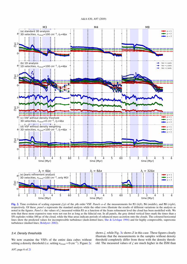
Figure 2a summarises the time evolution of the power-law indexζ(p) fit to the density-weighted VSF obtained for each cloud, andeach order p. The figure shows several interesting features. First,initially, at t = 0 Myr, all calculated values of ζ are above thepredicted values (see Eqs. (5) and (6)). This probably occurs pri-marily because the base simulation only resolves down to 0.49 pcbefore additional grid levels are added to resolve the clouds, soit cannot resolve the turbulence inertial range below approxi-mately 3 pc. This can be seen in the t = 0 Myr power spectrumin Fig. 25, Appendix B, of Paper II. As the zoom-in simula-tions evolve, the turbulence cascades to smaller scales in denseregions that are better resolved, so the density-weighted VSFslopes initially drop to the values expected for supersonic turbu-lence. The VSFs without density-weighting and, even more so,without density threshold remain too steep despite the increasedresolution in dense regions, because these VSFs remain domi-nated by numerical diffusion in the diffuse gas that has not beenfurther refined.
Second, ζ for all orders decreases with time as the cloudsare first refined and then begin to gravitationally collapse. Dis-tributed gravitational collapse causes an increase in relativevelocities at increasingly small scales as material falls into fil-aments and nodes. The increase in small-scale power leads toa flattening or even inversion of the VSF and thus a decreasein ζ. Third, occasionally one observes bumps and dips in slopein all orders of VSFs (e.g. M3 or M8 around t = 1.7 Myr). Thesefeatures only last for short periods of time (up to 0.6 Myr), butset in rather abruptly and represent sudden changes in large-scalepower that change the VSF slope.
Figure 3a shows the corresponding time evolution of theself-similarity parameter, Z. One sees that most of the timethe measured values of Z are in agreement or at least closelyapproaching the predicted values. The occasional peaks in Z (forexample, in M4 at t = 4.1 Myr) occur at times when the scalingexponents of the VSFs ζ(3) reach values close to or below 0.A decrease in Z (for example, in M3 around t = 1.8 Myr) occurswhen SN shocks hit and heavily impact the clouds, producingstronger effects in higher order VSFs.
We note that the nearby SNe that we mark in Figs. 2 and 3and consider in the analysis were listed by Paper II as explodingat a radius of up to 100 pc from the clouds’ centres of mass. Theshock fronts move at average speeds of 50–100 km s−1 throughthe ISM, so it can take the blast waves more than 1 Myr to reachthe clouds. Thus, it is important to keep in mind that the MCsdo not react immediately to SNe, and that the time between theexplosion of a SN and the interaction of its shock front with oneof the clouds varies depending on the distance, as well as withthe composition of the ISM along the propagation path.
Paper II discusses the influence of these SNe on the modelledclouds. In particular, the authors focus on the overall proper-ties of the clouds, like total mass, accretion rate, total velocitydispersion, and evolution. They find that there is a tight cor-relation between those properties and that the clouds evolutionstrongly depends on whether the clouds are hit by blast waves, aswell as the details of these interactions (meaning, for example,the strength or direction of the shock jump). Therefore, it isintuitive that blast waves have a substantial influence on the tur-bulence within the clouds, as well. We discuss this in more detailin the following sections of this paper.
In the rest of this section, we study how VSFs computed indifferent ways compare to these density weighted results. Wecompare the findings with the results we have obtained with ouroriginal setup. In Sect. 4, we discuss and interpret these resultsin more detail.
3.3. Line-of-sight VSF
Previously, we have seen how the VSF behaves and evolveswithin the clouds. To do this, we derived the relative velocitiesbased on the 3D velocity vectors from the simulations. How-ever, observed VSFs can only be measured using line-of-sightvelocities. In this subsection we investigate how VSFs derivedfrom 1D relative velocities compare to the 3D VSFs presentedbefore.
Figures 2b and 3b show measured ζ and Z, respectively,derived based on Eq. (8). We see that, in most of the cases, mostof the 1D VSFs agree well with each other, as well as with thecorresponding 3D VSFs. The VSFs of M4 are the best examplesfor this.
However, there are also cases in which the 1D VSF temporar-ily evolves completely differently than the 3D VSF. For example,the 1D VSF along the x-axis in M3 initially behaves like the cor-responding 3D VSF, though with lower absolute values of ζ(or higher values of Z). However, during the period t = 2.5–3.8 Myr the functions diverge. While the 3D ζ decreases furtherand switches sign, the ζ based on the 1D VSF along the x-axisshows a local maximum before converging with the 3D ζ again.Another example for temporal divergence are the VSFs ofM8 projected onto the x- and z-axes. Here, the VSFs developbelow or above the level of the 3D VSF, respectively. After theimpact of the SN blast wave at t = 1.5 Myr all three VSFs con-verge with each other, as well as with the 3D VSF under theinfluence of the on-going gravitational collapse.
A97, page 5 of 21
A&A 630, A97 (2019)
0
2
4
(p)
(a) standard 3D analysis3D velocities, ncloud=100 cm 3, J=4 x
M3 M4 M8p = 1p = 2p = 3
0
2
4
(p)
(b) 1D analysis1D velocities, ncloud=100 cm 3, J=4 x
los = x axislos = y axislos = z axis
0
2
4
(p)
(c) VSF without density theshold3D velocities, ncloud=0 cm 3, J=4 x
p = 1p = 2p = 3
0 1 2 3 4 5 6time [Myr]
0
2
4
(p)
(d) VSF without density weighting3D velocities, ncloud=100 cm 3, J=4 x
0 1 2 3 4 5 6time [Myr]
0 1 2 3 4 5 6time [Myr]
p = 1p = 2p = 3
0 1 2 3 4 5 6time [Myr]
0
2
4
(p)
(e) Jeans refinement analysis3D velocities, ncloud=100 cm 3, only M3!
J = 4 x
0 1 2 3 4 5 6time [Myr]
J = 8 x
0 1 2 3 4 5 6time [Myr]
J = 32 xp = 1p = 2p = 3
Fig. 2. Time evolution of scaling exponent ζ(p) of the pth order VSF. Panels a–d: the measurements for M3 (left), M4 (middle), and M8 (right),respectively. Of these, panel a represents the standard analysis while the other rows illustrate the results of different variations in the analysis asnoted in the figures. Panel e: the values of ζ measured within M3 as a function of the Jeans refinement level the cloud has been modelled with. Wenote that these more expensive runs were not run for as long as the fiducial run. In all panels, the grey dotted vertical lines mark the times than aSN explodes within 100 pc of the cloud, while the blue areas indicate periods of enhanced mass accretion onto the clouds. The coloured horizontallines show the predicted values for incompressible turbulence (dash-dotted lines; She & Lévêque 1994) and for highly compressible, supersonicturbulence (dashed lines; Boldyrev 2002).
3.4. Density thresholds
We now examine the VSFs of the entire data cubes withoutsetting a density threshold (i.e. setting ncloud = 0 cm−3). Figure 2c
shows ζ, while Fig. 3c shows Z in this case. These figures clearlyillustrate that the measurements in the samples without densitythreshold completely differ from those with the density thresh-old. The measured values of ζ are much higher in the ISM than
R.-A. Chira et al.: How do velocity structure functions trace gas dynamics in simulated molecular clouds?
0.5
0.0
0.5
1.0
1.5
Z(p)
(a) standard 3D analysis3D velocities, ncloud=100 cm 3, J=4 x
M3 M4 M8p = 1p = 2p = 3
0.5
0.0
0.5
1.0
1.5
Z(p)
(b) 1D analysis1D velocities, ncloud=100 cm 3, J=4 x
los = x axislos = y axislos = z axis
0.5
0.0
0.5
1.0
1.5
Z(p)
(c) VSF without density theshold3D velocities, ncloud=0 cm 3, J=4 x
p = 1p = 2p = 3
0 2 4 6time [Myr]
0.5
0.0
0.5
1.0
1.5
Z(p)
(d) VSF without density weighting3D velocities, ncloud=100 cm 3, J=4 x
0 2 4 6time [Myr]
0 2 4 6time [Myr]
p = 1p = 2p = 3
0 2 4 6time [Myr]
0
1
Z(p)
(e) Jeans refinement analysis3D velocities, ncloud=100 cm 3, only M3!
J = 4 x
0 2 4 6time [Myr]
J = 8 x
0 2 4 6time [Myr]
J = 32 xp = 1p = 2p = 3
Fig. 3. Like Fig. 2, but for the measured self-similarity parameter Z = ζ(p)/ζ(3) of the pth order VSF.
in the cloud-only sample. Although we see a slight decline of ζin M4 and M8 as the gas contracts under the influence of grav-ity in the vicinity of the clouds, ζ generally evolves differentlyhere than in the analysis that is focussed on the clouds, remain-ing very steep. We see a high rate of random fluctuations in theevolution of ζ, as well. Furthermore, contrary to all of our othertest scenarios, we see here that all Z are constant in time andwithin all clouds, with values slightly lower than those predictedby She & Lévêque (1994) for incompressible flows. This is con-sistent with the high sound speed in the hot gas that fills most of
the volume of the computational box, which results in subsonicflows predominating.
3.5. Density weighting
As mentioned in Sect. 2.2, Eq. (2) represents the definition of thedensity-weighted VSF. While this represents the observationalsituation better, the theoretical predictions were developed forthe unweighted statistic. Thus a comparison of results for the twovariations in our model is of interest. There are a few studies that
have targeted this question (e.g. Benzi et al. 1993, 2010; Schmidtet al. 2008; Gotoh et al. 2002). However, all of them consideredisotropic, homeogeneous, turbulent flows that are not compara-ble to our clouds. Padoan et al. (2016) use both methods, but noton the same set of data.
In this section, we investigate the influence of density weight-ing on VSFs by repeating the original analysis with the non-weighted VSF given by Eq. (2). Figures 2d and 3d show themeasured values of ζ and Z derived from the non-weightedVSFs, respectively.
Comparing the weighted and non-weighted samples, we seethe following: The non-weighted ζ (Fig. 2d) traces the interac-tions between the gas of the clouds and the SN shocks in thesame way as occurs for the density-weighted VSF. In M3 and M8we also see that the values of ζ decrease as the clouds evolve, yetnot as fast as they do in the density-weighted VSFs, which focusattention on the dense regions of strongest collapse. The mea-surements in M4, however, are almost constant over time. In allthe cases, the values of ζ never decrease below 0.5; a behaviourthat clearly differs from what we have observed in the density-weighted VSFs. The density weighting weakens the influence ofthe highly compressible flows in the densest regions, but not somuch as in the case with no density threshold. Consequently,the evolution of Zs (see Fig. 3d) becomes smoother, as well, asthere is no sign inversion of ζ. As a result the values of Z fluc-tuate slightly when shocks hit, and otherwise vary between thecompressible and incompressible limits.
3.6. Jeans length refinement
The results we have discussed so far are based on simulationdata presented in Paper I and Paper II. Due to the huge computa-tional expense of the variety of physical and numerical processes(fluid dynamics, adaptive mesh refinement, SNe, magnetic fields,radiative heating and cooling, and many more) within those sim-ulations, though, they have required some compromises. One ofthese compromises was the Jeans refinement criterion used aspart of the adaptive mesh refinement mechanism. The authorsresolved local Jeans lengths by only four zones (λJ = 4∆x). Thisis the minimal requirement for modelling self-gravitating gas indiscs in order to avoid artificial fragmentation (Truelove et al.1998). Other studies, have shown that a significantly higherrefinement is needed to reliably resolve turbulent structures andflows within discs to resolve turbulence (Federrath et al. 2011;Turk et al. 2012). In our case, the key question is how quickly theturbulent cascade fills in after the multiple steps of refinement tohigher resolution required to develop the high resolution cubeswe use. Although we have a different physical situation, the ear-lier results still emphasise the importance of how well the Jeanslength is resolved.
In the appendix of Paper II, the authors examine the effect thenumber of zones used for the Jeans refinement has on the mea-sured kinetic energy. For this, they have rerun the simulations ofM3 twice; once with λJ = 8∆x for the first 3 Myr after self-gravitywas activated, and once with λJ = 32∆x for the first megayear ofthe cloud’s evolution. The authors show that the λJ = 32∆x simu-lations smoothly recover the energy power spectrum on all scalesalready after this first megayear. The other two setups do this, aswell, but only over longer timescales (see also Paper II, Seifriedet al. 2017).
Furthermore, Paper II calculated the difference in the cloud’stotal kinetic energy as a function of time and refinement level.They found that the λJ = 4∆x simulations miss a significantamount of kinetic energy, namely up to 13% compared to
λJ = 8∆x and 33% compared to λJ = 32∆x. However, they alsoobserved that these differences peak around t = 0.5 Myr anddecrease afterwards, as the λJ = 4∆x and λJ = 8∆x simulationsadjust to the new refinement levels. Thus, the results we havederived from the λJ = 4∆x simulations need to be evaluated withrespect to this lack of turbulent energy, although the clouds’dynamics remains dominated by gravitational collapse. It alsomeans that the λJ = 4∆x data become more reliable the longerthe simulations evolve.
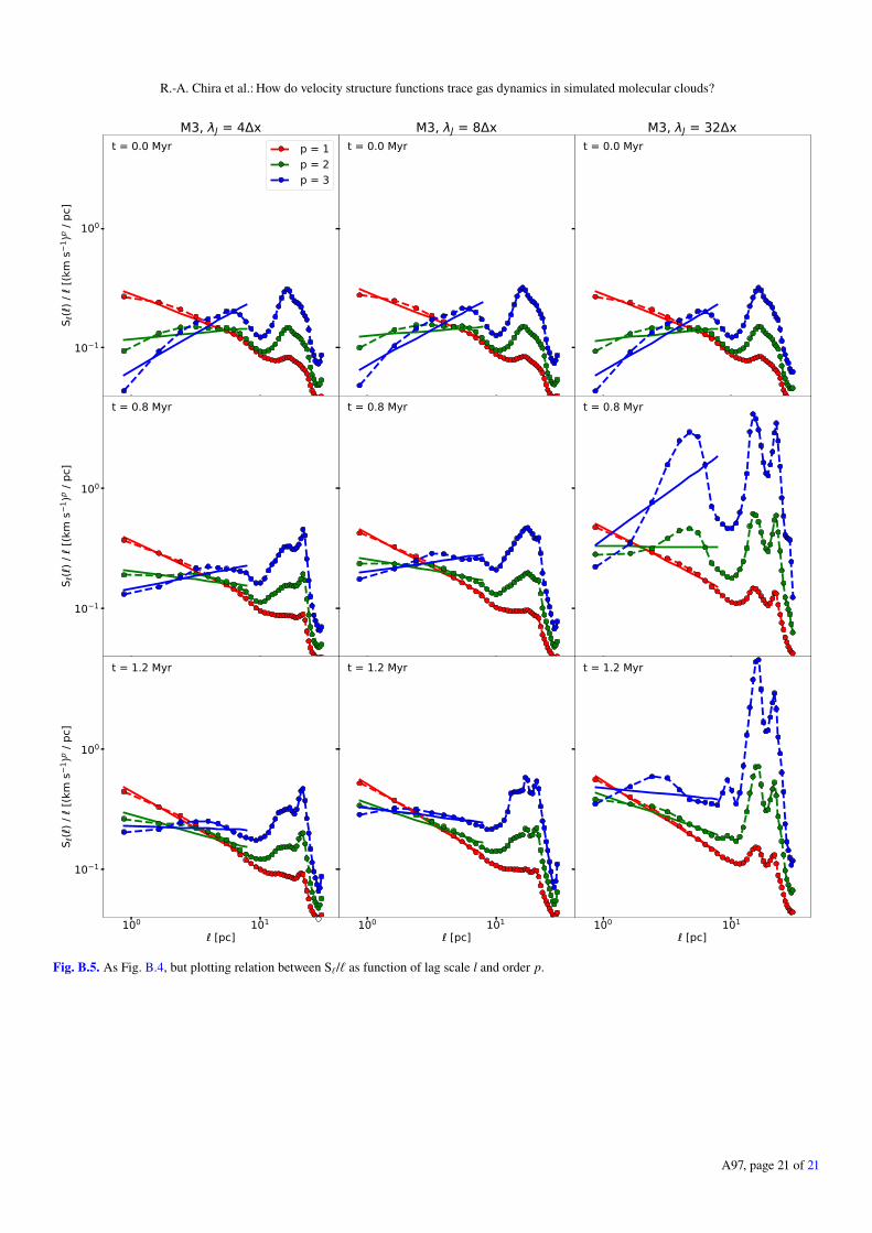
In order to study how the level of Jeans refinement influencesthe behaviour of the VSFs, we investigate the M3 data of theλJ = 8∆x and λJ = 32∆x simulations. Figures 2e and 3e show ζand Z for λJ = 8∆x and λJ = 32∆x. In Fig. 4 we directly comparethe measurements of all refinement levels relative to λJ = 4∆x.
The λJ = 8∆x model shows the same behaviour as λJ = 4∆x,with values in both samples being in good agreement as the toppanel of Fig. 4 demonstrates. Over the entire observed time span,the measured values of ζ decrease as the VSF become flatter. Atthe time the SNe interact with the cloud, over the course of abouta megayear after traveling across the distance from the point ofexplosion to the cloud, the VSFs steeply increase toward largerscales, causing values of ζ (Fig. 2e) to jump. Compared to theλJ = 4∆x sample, the peak in ζ is smoother and lasts longer athigher Jeans resolution.
These same effects can be seen in Fig. 3e where the drop of Zdue to the SN shock lasts longer than it did for λJ = 4∆x. Besidesthis, the time evolution of Z for λJ = 8∆x is as sensitive to theturbulence-related events as it was for λJ = 4∆x. The divergenceproduced when gravity has transferred the majority of power tosmaller scales occurs at the same time. The actual depth of thedrop is a numerical artefact caused by ζ(3) being equal or closeto zero at this very time step.
The picture changes when we analyse the VSFs based on theλJ = 32∆x runs (Figs. 2e, 3e, and 4). Here one sees that the mea-sured values of both ζ (Fig. 2e) and Z (Fig. 3e) are similar tothose for λJ = 4∆x for the first 0.2 Myr. After this short period,though, the evolution of ζ diverges. While ζ(1) and ζ(2) continueto decrease similar to λJ = 4∆x but at lower rate, ζ(3) increasesuntil it peaks at t = 0.8 Myr and falls steeply again. This diver-gence has notable impact on the evolution of Z, as well. Thebottom panel of Fig. 4 illustrates the different evolution of mea-sured ζ and Z in the two simulations more clearly. One sees thatthe differences between the samples follow the same pattern forall orders of p. The differences, though, increase with the order:While the values for ζ(1) are still in good agreement, the mea-sured values of ζ(2) and ζ(3) for λJ = 32∆x are 40% and 100%higher than those measured for λJ = 4∆x, respectively. Conse-quently, this causes differences in Z(p) of 30–52% between thesimulations. At t = 1.2 Myr, the last time step of this sample, thevalues of all ζ equal the measurements of λJ = 4∆x again. Asthe cost of extending the λJ = 32∆x simulation is prohibitive, wecannot determine whether this agreement will continue.
4. Discussion
4.1. Time evolution
We have seen in Sect. 3 that density-weighted VSFs reflecta combination of uniform, compressible turbulence, large-scale shocks, and gravitational collapse. Extended self-similarityemphasises the turbulent nature of these high-Reynolds numbersflows even in regions of gravitational collapse. The measuredvalues of ζ differ from the predicted values by She & Lévêque(1994) and Boldyrev (2002) for most of the time of the clouds’
A97, page 8 of 21
R.-A. Chira et al.: How do velocity structure functions trace gas dynamics in simulated molecular clouds?
0.5 0.0 0.5 1.0 1.5 2.0 2.5 3.0 3.5(p), J = 4 x
0
1
2
3
(p),
J = 8
x
0.0 0.2 0.4 0.6 0.8 1.0 1.2Z(p), J = 4 x
0.0
0.2
0.4
0.6
0.8
1.0
1.2
Z(p)
, J =
8x
0.5 0.0 0.5 1.0 1.5 2.0 2.5 3.0 3.5(p), J = 4 x
0
1
2
3
(p),
J = 3
2x
0.0 0.2 0.4 0.6 0.8 1.0 1.2Z(p), J = 4 x
0.0
0.2
0.4
0.6
0.8
1.0
1.2
Z(p)
, J =
32
x
Fig. 4. Comparison of VSF scaling exponents, ζ (left), and self-similarity parameters, Z (right), depending on the Jeans refinement of the simulationruns the data are based on. The abscissas give values from λJ = 4∆x, while the ordinates give values from λJ = 8∆x (top) and λJ = 32∆x (bottom).All data points refer to the M3 cloud and represent different lags in the same time step in the respective simulations.
evolution. The origin of these differences are to be found in acombination of numerical dissipation and the underlying phys-ical conditions. Contrary to the conditions in the referencemodels, we examine a multi-phase medium with magnetisedturbulence that is hardly uniform, isothermal, or homogeneous.However, the diffuse medium is also underresolved comparedto the dense gas, thanks to our Jeans refinement strategy, whichremoves small-scale power in the diffuse medium.
The impact of SN shocks hitting the clouds is to inject powerat all scales (Fig. 1). The resulting VSFs tend to lose their power-law character. Fitting a power-law to them anyway results insubstantial perturbations from the predictions for compressibleturbulence even under extended self-similarity. Figure 3 showstimes of SN explosions and periods of strong accretion onto theclouds. Remembering that it can take the shock front more than1 Myr to propagate from the site of the SN explosion to themolecular cloud, perturbations in Z not associated with zero-crossings by ζ(3) are consistent with being caused by SN shockfront interactions with the clouds. These shock interactions lastfor only a fraction of a megayear, though, consistent with thecrossing time of the blast wave through the dense interior ofthe cloud, after which the turbulent nature of the flow reassertsitself.
As the clouds gravitationally collapse, the resulting increasein small-scale power flattens or even inverts the density-weightedVSFs, resulting in decreasing or even negative values of ζ(Fig. 2a). The increase in small-scale power can also be derivedfrom the increasingly negative binding energy of the clouds asfurther gas falls into them Paper II. At the same time as theturbulence becomes increasingly non-uniform and anisotropicbecause of the importance of gravitation, the bulk velocity dis-persion of the cloud increases. Paper I showed that Eq. (1) issatisfied at these late times, but not at early times, less thana free-fall time, when the velocity dispersion inherited fromthe background turbulent flow is independent of the size of thecloud. These early times are when the turbulence dominates the
flow and the second-order power law is roughly ζ(2)' 1/2. Thissuggests that the apparent agreement with Larson’s size-velocityrelationship is coincidental. Observing two-point correlationsusing a method that cannot capture the dense flows adequatelywill yield this result from the cloud envelopes, though, thus per-haps explaining the apparent success of such efforts (Goodmanet al. 1998, Fig. 9 shows how these different interpretations canarise).
Extended self-similarity shows VSF ratios characteristic ofcompressible turbulence (Fig. 3a), as can be seen from their tend-ing to lie between the incompressible limit of She & Lévêque(1994) and the extremely compressible Burgers turbulence limitof Boldyrev (2002). (The extended self-similarity procedure failsas ζ(3) passes through zero, however, so it must be interpreted inconcert with the raw values of ζ.) This suggests that, just as theextended self-similarity procedure removes the effects of dissi-pation, it also removes the effects of hierarchical gravitationalcollapse, while continuing to reflect the turbulence in these highReynolds-numbers flows.
4.2. Line-of-sight velocities
In Sect. 3.3 we have seen that the ζ and Z derived from the1D VSFs generally evolve similarly to those derived from the3D VSFs. Yet, we have also seen that individual sight linesmay evolve differently. These differences appear to reflect thedetailed geometry of shock impacts on the cloud, which arereflected more strongly in the higher-order VSFs. For example,for the first 2 Myr of the evolution of M4 the values of Z alongthe y-axis are significantly higher than those observed along theother axes and diverge significantly from the values expected foruniform turbulence. It should be recalled here a perturbation inZ usually corresponds to an episode of strong shock driving,suggesting an impact along the y-axis at this time. Along theother two axes, Z continues to agree with supersonic turbulence(Boldyrev 2002). This effect is only visible as we analyse the
three dimensions separately, while the driving of the gas alongthe y-axis is averaged out in the 3D VSFs (see Fig. 3a).
In summary, for a fully developed 3D turbulent field weexpect that 1D VSFs behave similarly to 3D VSFs. However,when there is a preferred direction along which the gas flows,the 1D and 3D VSFs differ significantly from each other. Thus,we predict that observed VSFs reflect the nature of turbulencewithin MCs unless there is clear evidence that the gas is drivenin a particular direction (e.g. by a stellar wind or SN shock front).
We note that this analysis does not take typical line-of-sighteffects, such as optical depth or blending, into account. Futurestudies need to investigate this point in more detail by performingVSF analyses based on full radiative transfer calculations.
4.3. Density thresholds
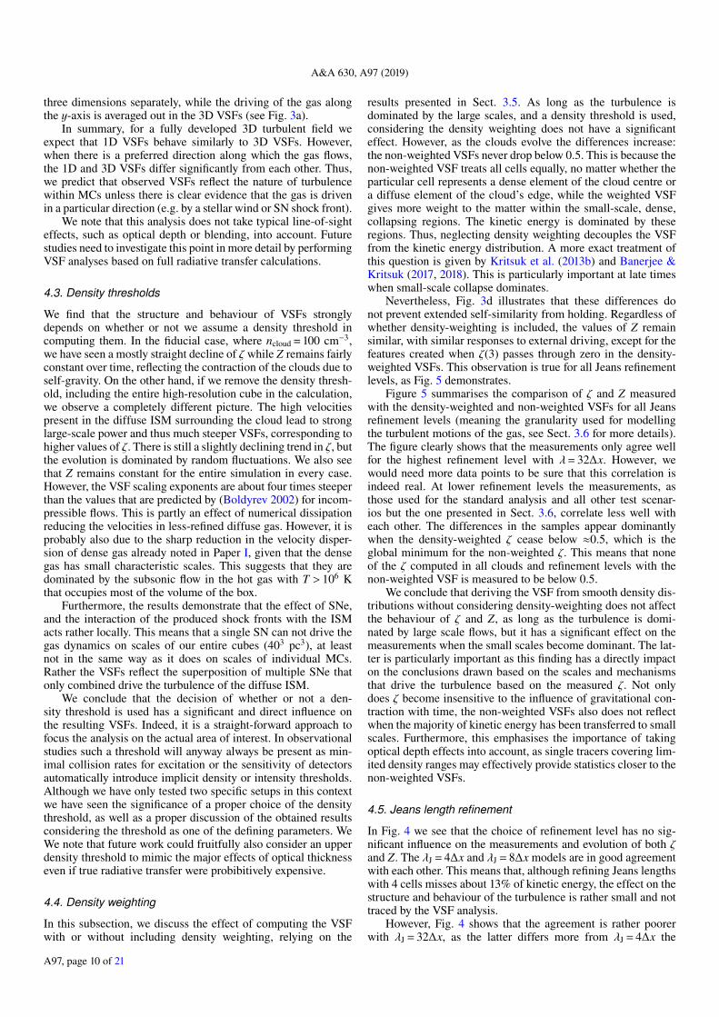
We find that the structure and behaviour of VSFs stronglydepends on whether or not we assume a density threshold incomputing them. In the fiducial case, where ncloud = 100 cm−3,we have seen a mostly straight decline of ζ while Z remains fairlyconstant over time, reflecting the contraction of the clouds due toself-gravity. On the other hand, if we remove the density thresh-old, including the entire high-resolution cube in the calculation,we observe a completely different picture. The high velocitiespresent in the diffuse ISM surrounding the cloud lead to stronglarge-scale power and thus much steeper VSFs, corresponding tohigher values of ζ. There is still a slightly declining trend in ζ, butthe evolution is dominated by random fluctuations. We also seethat Z remains constant for the entire simulation in every case.However, the VSF scaling exponents are about four times steeperthan the values that are predicted by (Boldyrev 2002) for incom-pressible flows. This is partly an effect of numerical dissipationreducing the velocities in less-refined diffuse gas. However, it isprobably also due to the sharp reduction in the velocity disper-sion of dense gas already noted in Paper I, given that the densegas has small characteristic scales. This suggests that they aredominated by the subsonic flow in the hot gas with T > 106 Kthat occupies most of the volume of the box.
Furthermore, the results demonstrate that the effect of SNe,and the interaction of the produced shock fronts with the ISMacts rather locally. This means that a single SN can not drive thegas dynamics on scales of our entire cubes (403 pc3), at leastnot in the same way as it does on scales of individual MCs.Rather the VSFs reflect the superposition of multiple SNe thatonly combined drive the turbulence of the diffuse ISM.
We conclude that the decision of whether or not a den-sity threshold is used has a significant and direct influence onthe resulting VSFs. Indeed, it is a straight-forward approach tofocus the analysis on the actual area of interest. In observationalstudies such a threshold will anyway always be present as min-imal collision rates for excitation or the sensitivity of detectorsautomatically introduce implicit density or intensity thresholds.Although we have only tested two specific setups in this contextwe have seen the significance of a proper choice of the densitythreshold, as well as a proper discussion of the obtained resultsconsidering the threshold as one of the defining parameters. WeWe note that future work could fruitfully also consider an upperdensity threshold to mimic the major effects of optical thicknesseven if true radiative transfer were probibitively expensive.
4.4. Density weighting
In this subsection, we discuss the effect of computing the VSFwith or without including density weighting, relying on the
results presented in Sect. 3.5. As long as the turbulence isdominated by the large scales, and a density threshold is used,considering the density weighting does not have a significanteffect. However, as the clouds evolve the differences increase:the non-weighted VSFs never drop below 0.5. This is because thenon-weighted VSF treats all cells equally, no matter whether theparticular cell represents a dense element of the cloud centre ora diffuse element of the cloud’s edge, while the weighted VSFgives more weight to the matter within the small-scale, dense,collapsing regions. The kinetic energy is dominated by theseregions. Thus, neglecting density weighting decouples the VSFfrom the kinetic energy distribution. A more exact treatment ofthis question is given by Kritsuk et al. (2013b) and Banerjee &Kritsuk (2017, 2018). This is particularly important at late timeswhen small-scale collapse dominates.
Nevertheless, Fig. 3d illustrates that these differences donot prevent extended self-similarity from holding. Regardless ofwhether density-weighting is included, the values of Z remainsimilar, with similar responses to external driving, except for thefeatures created when ζ(3) passes through zero in the density-weighted VSFs. This observation is true for all Jeans refinementlevels, as Fig. 5 demonstrates.
Figure 5 summarises the comparison of ζ and Z measuredwith the density-weighted and non-weighted VSFs for all Jeansrefinement levels (meaning the granularity used for modellingthe turbulent motions of the gas, see Sect. 3.6 for more details).The figure clearly shows that the measurements only agree wellfor the highest refinement level with λ= 32∆x. However, wewould need more data points to be sure that this correlation isindeed real. At lower refinement levels the measurements, asthose used for the standard analysis and all other test scenar-ios but the one presented in Sect. 3.6, correlate less well witheach other. The differences in the samples appear dominantlywhen the density-weighted ζ cease below ≈0.5, which is theglobal minimum for the non-weighted ζ. This means that noneof the ζ computed in all clouds and refinement levels with thenon-weighted VSF is measured to be below 0.5.
We conclude that deriving the VSF from smooth density dis-tributions without considering density-weighting does not affectthe behaviour of ζ and Z, as long as the turbulence is domi-nated by large scale flows, but it has a significant effect on themeasurements when the small scales become dominant. The lat-ter is particularly important as this finding has a directly impacton the conclusions drawn based on the scales and mechanismsthat drive the turbulence based on the measured ζ. Not onlydoes ζ become insensitive to the influence of gravitational con-traction with time, the non-weighted VSFs also does not reflectwhen the majority of kinetic energy has been transferred to smallscales. Furthermore, this emphasises the importance of takingoptical depth effects into account, as single tracers covering lim-ited density ranges may effectively provide statistics closer to thenon-weighted VSFs.
4.5. Jeans length refinement
In Fig. 4 we see that the choice of refinement level has no sig-nificant influence on the measurements and evolution of both ζand Z. The λJ = 4∆x and λJ = 8∆x models are in good agreementwith each other. This means that, although refining Jeans lengthswith 4 cells misses about 13% of kinetic energy, the effect on thestructure and behaviour of the turbulence is rather small and nottraced by the VSF analysis.
However, Fig. 4 shows that the agreement is rather poorerwith λJ = 32∆x, as the latter differs more from λJ = 4∆x the
A97, page 10 of 21
R.-A. Chira et al.: How do velocity structure functions trace gas dynamics in simulated molecular clouds?
0 1 2 3(p), J = 4 x, with
0.5
0.0
0.5
1.0
1.5
2.0
2.5
3.0
3.5
(p),
J = 4
x, w
ithou
t
0 1 2 3(p), J = 8 x, with
0.5
0.0
0.5
1.0
1.5
2.0
2.5
3.0
3.5
(p),
J = 8
x, w
ithou
t
0 1 2 3(p), J = 32 x, with
0.5
0.0
0.5
1.0
1.5
2.0
2.5
3.0
3.5
(p),
J = 3
2x,
with
out
0.5 0.0 0.5 1.0 1.5Z(p), J = 4 x, with
0.5
0.0
0.5
1.0
1.5
Z(p)
, J =
4x,
with
out
0.5 0.0 0.5 1.0 1.5Z(p), J = 8 x, with
0.5
0.0
0.5
1.0
1.5
Z(p)
, J =
8x,
with
out
0.5 0.0 0.5 1.0 1.5Z(p), J = 32 x, with
0.5
0.0
0.5
1.0
1.5
Z(p)
, J =
32
x, w
ithou
tp = 1p = 2p = 3
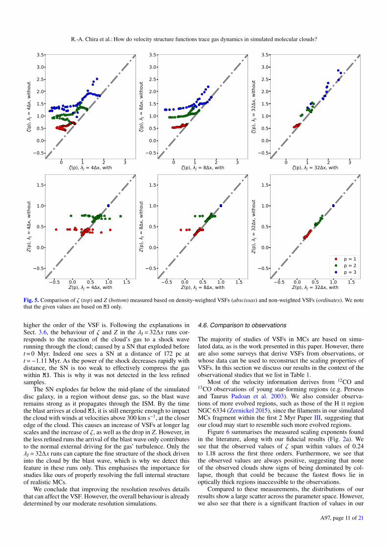
Fig. 5. Comparison of ζ (top) and Z (bottom) measured based on density-weighted VSFs (abscissas) and non-weighted VSFs (ordinates). We notethat the given values are based on M3 only.
higher the order of the VSF is. Following the explanations inSect. 3.6, the behaviour of ζ and Z in the λJ = 32∆x runs cor-responds to the reaction of the cloud’s gas to a shock waverunning through the cloud; caused by a SN that exploded beforet = 0 Myr. Indeed one sees a SN at a distance of 172 pc att =−1.11 Myr. As the power of the shock decreases rapidly withdistance, the SN is too weak to effectively compress the gaswithin M3. This is why it was not detected in the less refinedsamples.
The SN explodes far below the mid-plane of the simulateddisc galaxy, in a region without dense gas, so the blast waveremains strong as it propagates through the ISM. By the timethe blast arrives at cloud M3, it is still energetic enough to impactthe cloud with winds at velocities above 300 km s−1, at the closeredge of the cloud. This causes an increase of VSFs at longer lagscales and the increase of ζ, as well as the drop in Z. However, inthe less refined runs the arrival of the blast wave only contributesto the normal external driving for the gas’ turbulence. Only theλJ = 32∆x runs can capture the fine structure of the shock driveninto the cloud by the blast wave, which is why we detect thisfeature in these runs only. This emphasises the importance forstudies like ours of properly resolving the full internal structureof realistic MCs.
We conclude that improving the resolution resolves detailsthat can affect the VSF. However, the overall behaviour is alreadydetermined by our moderate resolution simulations.
4.6. Comparison to observations
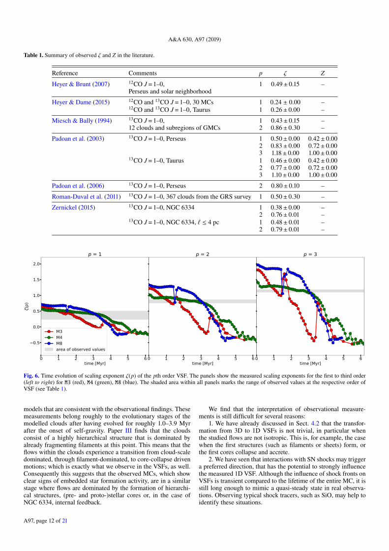
The majority of studies of VSFs in MCs are based on simu-lated data, as is the work presented in this paper. However, thereare also some surveys that derive VSFs from observations, orwhose data can be used to reconstruct the scaling properties ofVSFs. In this section we discuss our results in the context of theobservational studies that we list in Table 1.
Most of the velocity information derives from 12CO and13CO observations of young star-forming regions (e.g. Perseusand Taurus Padoan et al. 2003). We also consider observa-tions of more evolved regions, such as those of the H II regionNGC 6334 (Zernickel 2015), since the filaments in our simulatedMCs fragment within the first 2 Myr Paper III, suggesting thatour cloud may start to resemble such more evolved regions.
Figure 6 summarises the measured scaling exponents foundin the literature, along with our fiducial results (Fig. 2a). Wesee that the observed values of ζ span within values of 0.24to 1.18 across the first three orders. Furthermore, we see thatthe observed values are always positive, suggesting that noneof the observed clouds show signs of being dominated by col-lapse, though that could be because the fastest flows lie inoptically thick regions inaccessible to the observations.
Compared to these measurements, the distributions of ourresults show a large scatter across the parameter space. However,we also see that there is a significant fraction of values in our
13CO J = 1–0, NGC 6334, ` ≤ 4 pc 1 0.48± 0.01 –2 0.79± 0.01 –
0 1 2 3 4 5 6time [Myr]
0.5
0.0
0.5
1.0
1.5
2.0
(p)
p = 1
M3M4M8area of observed values
0 1 2 3 4 5 6time [Myr]
p = 2
0 1 2 3 4 5 6time [Myr]
p = 3
Fig. 6. Time evolution of scaling exponent ζ(p) of the pth order VSF. The panels show the measured scaling exponents for the first to third order(left to right) for M3 (red), M4 (green), M8 (blue). The shaded area within all panels marks the range of observed values at the respective order ofVSF (see Table 1).
models that are consistent with the observational findings. Thesemeasurements belong roughly to the evolutionary stages of themodelled clouds after having evolved for roughly 1.0–3.9 Myrafter the onset of self-gravity. Paper III finds that the cloudsconsist of a highly hierarchical structure that is dominated byalready fragmenting filaments at this point. This means that theflows within the clouds experience a transition from cloud-scaledominated, through filament-dominated, to core-collapse drivenmotions; which is exactly what we observe in the VSFs, as well.Consequently this suggests that the observed MCs, which showclear signs of embedded star formation activity, are in a similarstage where flows are dominated by the formation of hierarchi-cal structures, (pre- and proto-)stellar cores or, in the case ofNGC 6334, internal feedback.
We find that the interpretation of observational measure-ments is still difficult for several reasons:
1. We have already discussed in Sect. 4.2 that the transfor-mation from 3D to 1D VSFs is not trivial, in particular whenthe studied flows are not isotropic. This is, for example, the casewhen the first structures (such as filaments or sheets) form, orthe first cores collapse and accrete.
2. We have seen that interactions with SN shocks may triggera preferred direction, that has the potential to strongly influencethe measured 1D VSF. Although the influence of shock fronts onVSFs is transient compared to the lifetime of the entire MC, it isstill long enough to mimic a quasi-steady state in real observa-tions. Observing typical shock tracers, such as SiO, may help toidentify these situations.
R.-A. Chira et al.: How do velocity structure functions trace gas dynamics in simulated molecular clouds?
3. We have neglected typical line-of-sight effects that mayhave a significant influence on the measurements of the localstandard of rest velocity whose precision is crucial for this kindof study. Our projections ignore optical depth effects, and reflectvelocities all the way through the clouds, including high col-umn density regions of dynamical collapse where motions arefast at small scales. However, both 12CO and 13CO reach opti-cal depth of unity at relatively low column densities. This meansthat the observed VSFs will only reflect the motions of the sur-face layers of dense MCs. Figure 2, as well as the figures inAppendix A demonstrate that neglecting certain regimes, in par-ticular at small scales where column densities are highest, doeshave significant influence on the shape and scaling of the cor-responding VSF. Therefore, single-tracer observations are notsuitable for studying the dynamical structure of MCs. For aproper VSF analysis it would be advisable to use a variety oftracers to cover the different phases of the clouds, as well as topopulate the statistics of lag distances more completely.
4. Only a small fraction of the listed observational studiesin Table 1 aimed to measure the VSFs of the respective objectsdirectly. In the majority of cases, the focus of the investigationswas on the general budget of kinetic energy within the MC, aswell as the question whether those clouds follow Larson’s size-velocity relation (Eq. (1)). It is unclear whether the differencebetween a relation of the lag distance of two particles and theirrelative line-of-sight velocity and the connection between thesize of the entire MC and the velocity dispersion of the containedgas has always been considered.
We recommend that both theorists and observers discussin more detail how observational studies may use VSFs in thefuture. From the theoretical point-of-view, full line radiativetransfer calculations are required to better evaluate observationalbiases and simple projection effects. This requires observationswith a high spatial resolution of the respective MC for a widerange of lag scales and good statistics for fitting the scaling ofVSF, as well as lines with well-defined line-of-sight velocities,ideally, optically thin lines of intermediate- and high-densitytracers.
5. Summary and conclusions
In this paper, we analyse the VSFs of MCs that have formedwithin 3D magnetohydrodynamical, adaptive mesh refinement,FLASH simulations of the self-gravitating, SN-driven ISM byPaper II, including both density weighting and a density cutoff.The main results are as follows.1. The scaling of the density-weighted VSFs depends on a com-
bination of turbulence and more coherent processes such asSN blast wave impacts and gravitational contraction. We findthat the power-law scaling ζ of 3D density-weighted VSFsreflects the development of gravitational contraction, whilethe extended self-similarity scaling Z reveals interactions ofclouds with large-scale blast waves.
2. The two different proposed explanations for Larson’s size-velocity relationship, a turbulent cascade and gravitationalcontraction, appear to apply to different stages in the evolu-tion of MCs, as well as different observational techniques. Itappears coincidental that they have the same functional rela-tionship of length to velocity, which has led to confusion ofone with the other.
– MCs dominated by uniform turbulence show a first-order VSF with ζ(1) ' 1/2. The same result can be foundfor clouds undergoing strong gravitational contraction bycomputing the VSF without density weighting (or, most
likely, in the presence of optical depth effects), which isdominated by the low-density, turbulence-dominated outerregions of clouds. At the initial time, though, we mea-sure values of ζ(2) = 1 or larger in the density-weightedVSFs, that are inconsistent with turbulence models or sim-ulations that predict ζ(2) = 0.74 (Eq. (6)). However, theseinitial values are affected by numerical dissipation and tendto decrease as the resolution in dense regions increases in thezoom-in runs.
– Examining the overall velocity dispersion of gravi-tationally dominated clouds undergoing star formation, onthe other hand, reflects the dynamics of gravitational col-lapse. In this case, the cloud shows a shallow or eveninverted VSF dependence ζ(1). 0. This reflects strong flowsat small scales. However, such gravitationally contractingclouds were shown by Paper I to have an overall square-root velocity-radius relationship (Eq. (1)) given by free-fallor virial equilibrium (which differ by only 21/2, as noted byBallesteros-Paredes et al. 2011b).
3. As long as the MC is not affected by a shock, Z agreeswell with predicted values for supersonic flows, even asgravitational collapse proceeds.
4. We test the influence of Jeans refinement on the VSFs. Wefind that the absolute amount of kinetic energy does notinfluence the evolution of ζ and Z, but that better resolutionof external shocks can produce changes in both quantities.
5. Comparison of 3D to 1D VSFs shows differences in detail,but qualitative agreement in the behaviour of both ζ and Z,in particular when gravity dominates gas dynamics. Thus,observed 1D VSFs can be useful diagnostics in gravita-tionally bound and contracting regions. On the other hand,differences arise when strong transverse flows or shocksdominate the velocity field.
6. We calculate cloud VSFs using a density threshold to isolatethe cloud material, as would characteristically happen in anobservation of molecular material. Without such a thresh-old, our VSFs are dominated by the diffuse ISM. In thatcase, the extended self-similarity scaling Z lies just belowthe value predicted for isotropic, incompressible turbulenceby She & Lévêque (1994). This is consistent with the lowMach number in the hot, diffuse, ISM filling most of thevolume of our simulation. Yet, the actual values of ζ in thelow density gas are about four times higher than those pre-dicted by both She & Lévêque (1994) and Boldyrev (2002)due to some combination of numerical dissipation and themultiphase nature of the medium, which reduces velocitiesat small scale in dense regions (see Sect. 4.3).
7. We investigate the influence of defining the VSF with andwithout density weighting. We find that the qualitativebehaviour is traced by both approaches. However, the scal-ing of the non-weighted VSF ζ is always positive, not fallingnearly as far as for the density-weighted VSF. The density-weighted VSF reflects the kinetic energy distribution betteras gravitational collapse proceeds to smaller and smallerscales. (We note that in, for example, CO observations,optical depth effects may obscure this behaviour.)
8. We compare our results with measurements of both ζ and Zin observational studies. We see that our findings are gener-ally consistent with with observations within periods duringwhich the clouds’ flows are influenced by both turbulentflows and global gravitational contraction, including strongstructure formation and starting fragmentation. This reflectsthe conditions of embedded star formation activity withinobserved MCs.
A97, page 13 of 21
A&A 630, A97 (2019)
Our analysis shows that VSFs are useful tools for examining thedriving source of turbulence within MCs. However, studies thatuse VSFs need to precisely review the assumptions and param-eters included in their analysis as these can have a significantinfluence on the results.
For our simulated clouds, the VSFs illustrate that gravita-tional contraction dominates the evolution of the clouds. Duringcontraction, the VSF scaling exponent ζ(p) drops in value andcan even become negative as kinetic energy concentrates onsmall scales. Nevertheless, the extended self-similarity scalingparameters Z(p) continue to agree with the analytic predic-tion for compressible turbulence except for short periods dur-ing which SN blast waves increase power on multiple scales.Because such blast waves are neither homogeneous nor isotropic,they often lead to transient non-power law scaling of the VSFs,and thus strong departures from uniform turbulent behaviour ofZ(p).
Acknowledgements. We thank the anonymous referee for a detailed report thatled to an improved and better focussed exposition, particularly in the discus-sion of Larson’s relation, as well as the inclusion of the Appendices. M.-M.M.L.received support from US NSF grants AST11-09395 and AST18-15461, andthanks the A. von Humboldt-Stiftung for support. J.C.I.-M. was additionally sup-ported by the Deutsche Forschungsgemeinschaft (DFG) via the CollaborativeResearch Center SFB 956 “Conditions and Impact of Star Formation” (subpro-ject C5) and the DFG Priority Program 1573 “The physics of the interstellarmedium”.
ReferencesBallesteros-Paredes, J., Hartmann, L. W., Vázquez-Semadeni, E., Heitsch, F., &
Zamora-Avilés, M. A. 2011a, MNRAS, 411, 65Ballesteros-Paredes, J., Vázquez-Semadeni, E., Gazol, A., et al. 2011b, MNRAS,
416, 1436Banerjee, S., & Galtier, S. 2013, Phys. Rev. E, 87, 013019Banerjee, S., & Kritsuk, A. G. 2017, Phys. Rev. E, 96, 053116Banerjee, S., & Kritsuk, A. G. 2018, Phys. Rev. E, 97, 023107Benzi, R., Ciliberto, S., Tripiccione, R., et al. 1993, Phys. Rev. E, 48, R29Benzi, R., Biferale, L., Fisher, R., Lamb, D. Q., & Toschi, F. 2010, J. Fluid
Mech., 653, 221Boldyrev, S. 2002, ApJ, 569, 841Boneberg, D. M., Dale, J. E., Girichidis, P., & Ercolano, B. 2015, MNRAS, 447,
1341Brunt, C. M., & Heyer, M. H. 2013, MNRAS, 433, 117Brunt, C. M., Heyer, M. H., & Mac Low, M.-M. 2009, A&A, 504, 883Burkhart, B., Collins, D. C., & Lazarian, A. 2015, ApJ, 808, 48Chira, R.-A., Ibáñez-Mejía, J. C., Mac Low, M.-M., & Henning, T. 2018a, How
do Velocity Structure Functions Trace Gas Dynamics in Simulated MolecularClouds? (New York: American Museum of Natural History Research Library)
Chira, R.-A., Kainulainen, J., Ibáñez-Mejía, J. C., Henning, T., & Mac Low,M.-M. 2018b, A&A, 610, A62
Dekel, A., & Krumholz, M. R. 2013, MNRAS, 432, 455Elmegreen, B. G. 1993, in Protostars and Planets III, eds. E. H. Levy & J. I.
Lunine (Tucson: University of Arizona Press), 97Elmegreen, B. G. 2007, ApJ, 668, 1064Falgarone, E., Pety, J., & Hily-Blant, P. 2009, A&A, 507, 355Federrath, C., Sur, S., Schleicher, D. R. G., Banerjee, R., & Klessen, R. S. 2011,
ApJ, 731, 62Fleck, Jr. R. C. 1980, ApJ, 242, 1019Fryxell, B., Olson, K., Ricker, P., et al. 2000, ApJS, 131, 273Galtier, S., & Banerjee, S. 2011, Phys. Rev. Lett., 107, 134501Gnedin, O. 2015, IAU General Assembly, 22, 2256326Goodman, A. A., Barranco, J. A., Wilner, D. J., & Heyer, M. H. 1998, ApJ, 504,
223Gotoh, T., Fukayama, D., & Nakano, T. 2002, Phys. Fluids, 14, 1065Hartmann, L., Ballesteros-Paredes, J., & Heitsch, F. 2012, MNRAS, 420,
1457Heyer, M. H., & Brunt, C. M. 2004, ApJ, 615, L45Heyer, M. H., & Brunt, C. 2007, IAU Symp., 237, 9Heyer, M., & Dame, T. M. 2015, ARA&A, 53, 583Heyer, M., Krawczyk, C., Duval, J., & Jackson, J. M. 2009, ApJ, 699, 1092Ibáñez-Mejía, J. C., Mac Low, M.-M., Klessen, R. S., & Baczynski, C. 2016,
ApJ, 824, 41Ibáñez-Mejía, J. C., Mac Low, M.-M., Klessen, R. S., & Baczynski, C. 2017,
ApJ, 850, 62Kolmogorov, A. 1941, Akademiia Nauk SSSR Doklady, 30, 301Kritsuk, A. G., Lee, C. T., & Norman, M. L. 2013a, MNRAS, 436, 3247Kritsuk, A. G., Wagner, R., & Norman, M. L. 2013b, J. Fluid Mech., 729, R1Kritsuk, A. G., Wagner, R., & Norman, M. L. 2015, ASP Conf. Ser., 498, 16Krumholz, M. R., Bate, M. R., Arce, H. G., et al. 2014, Protostars and Planets VI
(Tucson: University of Arizona Press), 243Larson, R. B. 1981, MNRAS, 194, 809Mac Low, M.-M. 2003, in Turbulence and Magnetic Fields in Astrophysics, Lect.
Notes Phys., (Berlin: Springer Verlag), eds. E. Falgarone & T. Passot, 614,182
Mac Low, M.-M., & Klessen, R. S. 2004, Rev. Mod. Phys., 76, 125McKee, C. F., & Zweibel, E. G. 1992, ApJ, 399, 551Miesch, M. S., & Bally, J. 1994, ApJ, 429, 645Miyamoto, Y., Nakai, N., & Kuno, N. 2014, PASJ, 66, 36Padoan, P., Boldyrev, S., Langer, W., & Nordlund, Å. 2003, ApJ, 583,
308Padoan, P., Juvela, M., Kritsuk, A., & Norman, M. L. 2006, ApJ, 653,
194505Seifried, D., Walch, S., Girichidis, P., et al. 2017, MNRAS, 472, 4794She, Z.-S., & Lévêque, E. 1994, Phys. Rev. Lett., 72, 336Solomon, P. M., Rivolo, A. R., Barrett, J., & Yahil, A. 1987, ApJ, 319, 730Tan, J. C., Shaske, S. N., & Van Loo, S. 2013, IAU Symp., 292, 19Truelove, J. K., Klein, R. I., McKee, C. F., et al. 1998, ApJ, 495, 821Turk, M. J., Oishi, J. S., Abel, T., & Bryan, G. L. 2012, ApJ, 745, 154Vázquez-Semadeni, E., Ryu, D., Passot, T., González, R. F., & Gazol, A. 2006,
ApJ, 643, 245Zernickel, A. 2015, PhD Thesis, Köln, Germany
R.-A. Chira et al.: How do velocity structure functions trace gas dynamics in simulated molecular clouds?
Appendix A: Computation and fitting procedures
1.0
0.5
0.0
0.5
1.0
1.5
2.0
2.5
(p)
M3 M4 M8p = 3p = 2p = 1
0 1 2 3 4 5 6time [Myr]
1.0
0.5
0.0
0.5
1.0
1.5
2.0
2.5
Z(p)
0 1 2 3 4 5 6time [Myr]
0 1 2 3 4 5 6time [Myr]
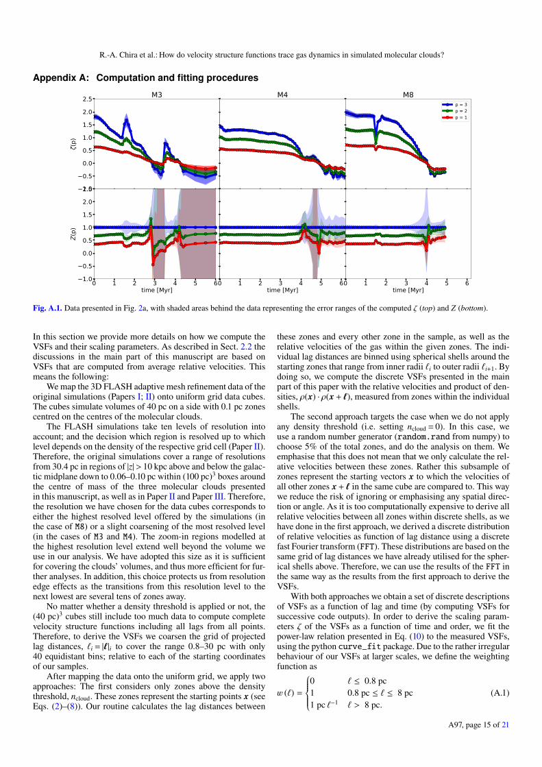
Fig. A.1. Data presented in Fig. 2a, with shaded areas behind the data representing the error ranges of the computed ζ (top) and Z (bottom).
In this section we provide more details on how we compute theVSFs and their scaling parameters. As described in Sect. 2.2 thediscussions in the main part of this manuscript are based onVSFs that are computed from average relative velocities. Thismeans the following:
We map the 3D FLASH adaptive mesh refinement data of theoriginal simulations (Papers I; II) onto uniform grid data cubes.The cubes simulate volumes of 40 pc on a side with 0.1 pc zonescentred on the centres of the molecular clouds.
The FLASH simulations take ten levels of resolution intoaccount; and the decision which region is resolved up to whichlevel depends on the density of the respective grid cell (Paper II).Therefore, the original simulations cover a range of resolutionsfrom 30.4 pc in regions of |z|> 10 kpc above and below the galac-tic midplane down to 0.06–0.10 pc within (100 pc)3 boxes aroundthe centre of mass of the three molecular clouds presentedin this manuscript, as well as in Paper II and Paper III. Therefore,the resolution we have chosen for the data cubes corresponds toeither the highest resolved level offered by the simulations (inthe case of M8) or a slight coarsening of the most resolved level(in the cases of M3 and M4). The zoom-in regions modelled atthe highest resolution level extend well beyond the volume weuse in our analysis. We have adopted this size as it is sufficientfor covering the clouds’ volumes, and thus more efficient for fur-ther analyses. In addition, this choice protects us from resolutionedge effects as the transitions from this resolution level to thenext lowest are several tens of zones away.
No matter whether a density threshold is applied or not, the(40 pc)3 cubes still include too much data to compute completevelocity structure functions including all lags from all points.Therefore, to derive the VSFs we coarsen the grid of projectedlag distances, `i = |`|i to cover the range 0.8–30 pc with only40 equidistant bins; relative to each of the starting coordinatesof our samples.
After mapping the data onto the uniform grid, we apply twoapproaches: The first considers only zones above the densitythreshold, ncloud. These zones represent the starting points x (seeEqs. (2)–(8)). Our routine calculates the lag distances between
these zones and every other zone in the sample, as well as therelative velocities of the gas within the given zones. The indi-vidual lag distances are binned using spherical shells around thestarting zones that range from inner radii `i to outer radii `i+1. Bydoing so, we compute the discrete VSFs presented in the mainpart of this paper with the relative velocities and product of den-sities, ρ(x) · ρ(x + `), measured from zones within the individualshells.
The second approach targets the case when we do not applyany density threshold (i.e. setting ncloud = 0). In this case, weuse a random number generator (random.rand from numpy) tochoose 5% of the total zones, and do the analysis on them. Weemphasise that this does not mean that we only calculate the rel-ative velocities between these zones. Rather this subsample ofzones represent the starting vectors x to which the velocities ofall other zones x + ` in the same cube are compared to. This waywe reduce the risk of ignoring or emphasising any spatial direc-tion or angle. As it is too computationally expensive to derive allrelative velocities between all zones within discrete shells, as wehave done in the first approach, we derived a discrete distributionof relative velocities as function of lag distance using a discretefast Fourier transform (FFT). These distributions are based on thesame grid of lag distances we have already utilised for the spher-ical shells above. Therefore, we can use the results of the FFT inthe same way as the results from the first approach to derive theVSFs.
With both approaches we obtain a set of discrete descriptionsof VSFs as a function of lag and time (by computing VSFs forsuccessive code outputs). In order to derive the scaling param-eters ζ of the VSFs as a function of time and order, we fit thepower-law relation presented in Eq. (10) to the measured VSFs,using the python curve_fit package. Due to the rather irregularbehaviour of our VSFs at larger scales, we define the weightingfunction as
Although the average radii of our clouds are, on aver-age, larger than 8 pc we choose this limit due to the variablebehaviour of the VSFs at scales of that size and larger. Investiga-tion of different weightings would be a fruitful topic of furtherinvestigation.
As can be seen in Fig. 1, as well as in the figures shown inAppendix B, the shape of VSFs changes over time as differentforces act, as we explain in Sect. 3. The similarity parameters,Z, are computed by applying Eq. (9) on the results of the fit-ting procedure, and results are presented in Sect. 3, as well as inAppendix B.
The fit also provides the χ2 errors for the measured valuesof ζ. In Fig. A.1 we show a reduced version of Fig. 2(a), wherewe only plot the time evolution of ζ for all three clouds, alongwith shades of the same colours of the respective lines that rep-resent the errors. We see that the relative errors, ∆ζ/ζ mostlyremain within a range of 5–12%. The errors of Z are computedby Gaussian error propagation
∆Z(p) =
√(∂Z(p)∂ζ(p)
· ∆ζ(p))2
+
(∂Z(p)∂ζ(3)
· ∆ζ(3))2
(A.2)
=
√(∆ζ(p)ζ(3)
)2
+
(ζ(p) · ∆ζ(3)
ζ(3)2
)2
. (A.3)
In general, the relative errors of Z are, as well, around 10%,though we do see exceptions with very large errors. The rea-son for these is that at these times ζ(3) approaches zero, causingEq. (A.3) to diverge.
Appendix B: Inertial range
For our analysis it is essential to verify that there is a reason-able range of scales ` below the driving range within whichthe simulations are not dominated by numerical effects, so thatthey resolve the inertial range of any turbulent cascade. We notethat the fitting region for our VSFs starts at lags greater thaneight zones, ensuring that the numerical dissipation range lies atsmaller scales. To understand the non-power law behaviour thatwe nonetheless find, in the following subsections we offer moreexamples that show VSFs of all three clouds at different timesand considering our different analysis approaches. We focus onthe standard analysis in Appendix B.1, on the analysis neglect-ing the density threshold in Appendix B.2, and on the impact ofvarying the resolution in collapsing regions in Appendix B.3.
B.1. Standard analysis
Figure B.1 extends the data presented in Sect. 3.2 and dis-cussed in Sect. 4.1. The figure uses the same format as Fig. 1.The straight lines within the plots indicate the power-law rela-tion that we have fitted onto the VSFs, considering the range0.8≤ `≤ 8 pc.
We see that in most of the cases the VSFs are in good agree-ment with the described power-law relation within the fittedranges (e.g. Fig. 1). However, there are cases when the VSF isnot well reproduced by a simple, single power-law function, suchas M3 at t = 3.0 Myr in Fig. 1. This appears to occur particularlywhen the dominant mechanism driving turbulence changes fromlarge-scale driving to internal contraction. At this point the largerscales of the clouds (larger `) are still dominated by external driv-ing, while the smaller scales (smaller `) start to accelerate mostlydue to gravitational fragmentation and infall motions. The conse-quence is that the actual VSF is a superposition of two processesthat amplify the relative motions of the gas differently and on dif-ferent scales. A single power-law cannot describe this scenarioadequately.
B.2. No density threshold
Figures B.2 and B.3 extend the set of VSFs for the box with-out a density threshold presented in Sect. 3.4 and discussed inSect. 4.3. Here we also find problems describing the behaviourof small-scale motions with `. 2 pc. In this case we primar-ily capture the turbulent motions within the low-density ISM.Contrary to the modelled MCs, the ISM is not organised inhierarchical structures, and the turbulence within the ISM is pre-dominantly driven by SN explosions. These produce structuredcorrelations at the large scales of entire blast waves as well asthe small scales across shock fronts. Yet, we see that we canfit the VSFs with a power law within the intermediate lag scaleranges (2 pc. `. 8 pc), suggesting this range of length scales isdominated by a turbulent cascade.
B.3. Varying refinement
Figures B.4 and B.5 extend the set of VSFs presented for cloudswith varying amounts of refinement in gravitationally collapsingregions in Sect. 3.6 and discussed in Sect. 4.5. A final exam-ple of VSFs not following a power law at intermediate scales isgiven by cloud M3 at t = 0.8 Myr and with λJ = 32∆x in Fig. B.4.This represents the VSF of a cloud that is interacting with aSN blast wave. In this case the maximal amplification is nei-ther at the scale of the cloud, where the turbulence is driven byexternal sources, nor on small scales where gravitational con-traction acts. Instead the local maximum is the intermediatescale. Considering the morphology of the cloud and the cloud’senvironment this can only occur when the shock front of a SN iscurrently propagating through the cloud. Thus, the VSF here isa superposition of three driving mechanisms: first, the externallarge-scale driving; second, self-gravity that leads to contractivemotions; and finally the shock jump that injects kinetic energyas it moves through the cloud. The effect of the shock, however,is only local and short-lived as the injected turbulence decaysquickly (compare with M3 at t = 1.2 Myr and with λJ = 32∆x inFig. B.4).
A97, page 16 of 21
R.-A. Chira et al.: How do velocity structure functions trace gas dynamics in simulated molecular clouds?
10 2
10 1
100
101
S()
/ [(
km s
1 )p /
pc]
t = 1.0 MyrM3
p = 1p = 2p = 3
t = 1.0 MyrM4
t = 1.0 MyrM8
10 2
10 1
100
101
S()
/ [(
km s
1 )p /
pc]
t = 3.0 Myr t = 3.0 Myr t = 3.0 Myr
100 101
[pc]10 2
10 1
100
101
S()
/ [(
km s
1 )p /
pc]
t = 4.2 Myr
100 101
[pc]
t = 4.2 Myr
100 101
[pc]
t = 4.2 Myr
Fig. B.1. As Fig. 1, but plotting relation between S`/` as function of lag scale l and order p.
Fig. B.4. Additional examples of VSFs, based on data of M3 with density threshold, at different refinement levels (left to right) λ= 4∆x, λ= 8∆x,and λ= 8∆x as function of lag scale ` and order p. The examples are given for three different time steps, namely (top to bottom) t = 0.0, 0.8, and1.2 Myr. The dots (connected by dashed lines) show the values computed from the simulations. The solid lines represent the power-law relationfitted to the respective structure functions.