How have house prices evolved in the longrun? This paper ...

econstorMake Your Publications Visible

A Service of

zbwLeibniz-InformationszentrumWirtschaftLeibniz Information Centrefor Economics

Knoll Katharina Schularick Moritz Steger Thomas

Working Paper

No Price Like Home Global House Prices1870-2012

CESifo Working Paper No 5006

Provided in Cooperation withIfo Institute ndash Leibniz Institute for Economic Research at the University of Munich

Suggested Citation Knoll Katharina Schularick Moritz Steger Thomas (2014) No Price LikeHome Global House Prices 1870-2012 CESifo Working Paper No 5006 Center for EconomicStudies and ifo Institute (CESifo) Munich

This Version is available athttphdlhandlenet10419103123

Standard-Nutzungsbedingungen

Die Dokumente auf EconStor duumlrfen zu eigenen wissenschaftlichenZwecken und zum Privatgebrauch gespeichert und kopiert werden

Sie duumlrfen die Dokumente nicht fuumlr oumlffentliche oder kommerzielleZwecke vervielfaumlltigen oumlffentlich ausstellen oumlffentlich zugaumlnglichmachen vertreiben oder anderweitig nutzen

Sofern die Verfasser die Dokumente unter Open-Content-Lizenzen(insbesondere CC-Lizenzen) zur Verfuumlgung gestellt haben solltengelten abweichend von diesen Nutzungsbedingungen die in der dortgenannten Lizenz gewaumlhrten Nutzungsrechte

Terms of use

Documents in EconStor may be saved and copied for yourpersonal and scholarly purposes

You are not to copy documents for public or commercialpurposes to exhibit the documents publicly to make thempublicly available on the internet or to distribute or otherwiseuse the documents in public

If the documents have been made available under an OpenContent Licence (especially Creative Commons Licences) youmay exercise further usage rights as specified in the indicatedlicence

wwweconstoreu

No Price Like Home Global House Prices 1870 - 2012

Katharina Knoll Moritz Schularick

Thomas Steger

CESIFO WORKING PAPER NO 5006 CATEGORY 6 FISCAL POLICY MACROECONOMICS AND GROWTH

OCTOBER 2014

An electronic version of the paper may be downloaded bull from the SSRN website wwwSSRNcom bull from the RePEc website wwwRePEcorg

bull from the CESifo website TwwwCESifo-grouporgwp T

Abstract How have house prices evolved in the long-run This paper presents annual house price indices for 14 advanced economies since 1870 Based on extensive data collection we are able to show for the first time that house prices in most industrial economies stayed constant in real terms from the 19th to the mid-20th century but rose sharply in recent decades Land prices not construction costs hold the key to understanding the trajectory of house prices in the long-run Residential land prices have surged in the second half of the 20th century but did not increase meaningfully before We argue that before World War II dramatic reductions in transport costs expanded the supply of land and suppressed land prices Since the mid-20th century comparably large land-augmenting reductions in transport costs no longer occurred Increased regulations on land use further inhibited the utilization of additional land while rising expenditure shares for housing services increased demand

JEL-Code N100 O100 R300 R400

Keywords house prices land prices transportation costs neoclassical theory

Katharina Knoll Free University of Berlin

Berlin Germany katharinaknollfu-berlinde

Moritz Schularick Institute of Macroeconomics and

Econometrics University of Bonn Adenauerallee 24-42

Germany ndash 53113 Bonn moritzschularickuni-bonnde

Thomas Steger

Leipzig University Leipzig Germany

stegerwifauni-leipzigde

corresponding author We wish to thank Klaus Adam Christian Bayer Jacques Friggit Volker Grossman Riitta Hjerppe Mathias Hoffmann Carl-Ludwig Holtfrerich Ogravescar Jordagrave Marvin McInnis Philip Jung Christopher Meissner Alexander Nuumltzenadel Thomas Piketty Jonathan D Rose Petr Sedladcek Sjak Smulders Kenneth Snowden Alan M Taylor Daniel Waldenstroumlm and Nikolaus Wolf for helpful discussions and comments Schularick received financial support from the Volkswagen Foundation Part of this research was undertaken while Knoll was at New York University Niklas Flamang Miriam Kautz and Hans Torben Loumlfflad provided excellent research assistance All remaining errors are our own

1 Introduction

For Dorothy there was no place like home But despite her ardent desire to get back to KansasDorothy probably had no idea how much her beloved home cost She was not aware that theprice of a standard Kansas house in the late 19th century was around 2400 dollars (Wickens1937) She could also not have known whether relocating the house to Munchkin Countrywould have increased its value or not For economists there is no price like home ndash at leastnot since the global financial crisis fluctuations in house prices their impact on the balancesheets of consumers and banks as well as the deleveraging pressures triggered by house pricebusts have been a major focus of macroeconomic research in recent years (Mian and Sufi 2014Shiller 2009 Case and Quigley 2008) In the context of business cycles the nexus betweenmonetary policy and the housing market has become a rapidly expanding research field (Adamand Woodford 2013 Goodhart and Hofmann 2008 Del Negro and Otrok 2007 Leamer2007) Houses are typically the largest component of household wealth the key collateral forbank lending and play a central role for long-run trends in wealth-to-income ratios and thesize of the financial sector (Piketty and Zucman 2014 Jordagrave et al 2014) Yet despite theirimportance for the macroeconomy surprisingly little is known about long-run trends in houseprices This paper aims to fill this void

Based on extensive historical research we present house price indices for 14 advancedeconomies since 1870 A large part of this paper is devoted to the presentation and discussion ofthe data that we unearthed from more than 60 different primary and secondary sources Thereare good reasons why we devote a great deal of (printer) ink and paper discussing the dataand their sources Houses are heterogeneous assets and when combining data from a varietyof sources great care is needed to construct plausible long-run indices that account for qualityimprovements shifts in the composition of the type of houses and their location We go intoconsiderable detail to test the robustness and corroborate the plausibility of the resulting houseprice data with additional historical sources

For the construction of the long-run database we were able to build in part on the existingwork of economic and financial historians such as Eichholtz (1994) for the Netherlands andEitrheim and Erlandsen (2004) for Norway In many other cases we collected new informationfrom regional and national statistical offices central banks as well as from tax authorities suchas the UK Land Registry or national real estate associations such as the Canadian Real EstateAssociation (1981) In addition to house price data we have also assembled for the first timecorresponding long-run data for construction costs farmland prices as well as expenditures onhousing services

Using the new dataset we are able to show that real house prices in the advanced economiessince the 19th century have taken a particular trajectory that to the best of our knowledgehas not yet been documented From the last quarter of the 19th to the mid-20th century house

2

prices in most industrial economies were largely constant in real terms By the 1960s they wereon average not much higher than they were on the eve of World War I They have been on along and pronounced ascent since then For our sample real house prices have approximatelytripled since the beginning of the 20th century with virtually all of the increase occurring in thesecond half of the 20th century We also find considerably cross-country heterogeneity WhileAustralia has seen the strongest Germany has seen the weakest increase in real house prices inthe long-run Moreover we demonstrate that urban and rural house prices have by and largemoved together and that long-run farmland prices exhibit a similar long-run pattern

We go one step further and study the driving forces of this hockey-stick pattern of houseprices Houses are bundles of the structure and the underlying land An accounting decompo-sition of house price dynamics into replacement costs of the structure and land prices demon-strates that rising land prices hold the key to understanding the upward trend in global houseprices While construction costs have flat-lined in the past decades sharp increases in residen-tial land prices have driven up international house prices Our decomposition suggests thatabout 80 percent of the increase in house prices between 1950 and 2012 can be attributed toland prices The pronounced increase in residential land prices in recent decades contrastsstarkly with the period from the late 19th to the mid-20th century During this period resi-dential land prices remained by and large constant in advanced economies despite substantialpopulation and income growth We are not the first to note the upward trend in land prices inthe second half of the 20th century (Glaeser and Ward 2009 Case 2007 Davis and Heathcote2007 Gyourko et al 2006) But to our knowledge it has not been shown that this is a broadbased cross-country phenomenon that marks a break with the previous era

How can one explain the fact that residential land prices remained stable until the mid-20th century and increased strongly in the past half-century We discuss this question boththeoretically and empirically Our emphasis is on the different dynamics in land supply beforeand after the middle of the 20th century From the 19th to the early 20th century the transportrevolution ndash mostly the construction of the railway network but also the introduction of steamshipping and cars ndash led to a massive and well-documented drop in transport costs often referredto as the transportation revolution (Jacks and Pendakur 2010 Taylor 1951) An importanteffect of the transport revolution was to substantially augment the supply of economicallyusable land We develop a model with land heterogeneity to demonstrate how a sustaineddecline in transport costs endogenously triggers an expansion of land such that the land pricemay remain low despite continuous growth of incomes and population We show that thisland-augmenting decline in transport costs subsides in the second half of the 20th centuryso that land increasingly became a fixed factor At the same time zoning regulations andother restrictions on land use also inhibited the utilization of additional land in recent decades(Glaeser et al 2005a Glaeser and Gyourko 2003) while rising expenditure shares for housingservices added further to the rising demand for land

3

Our findings also have potentially important implications for the much debated issue oflong-run trends in distribution of income and wealth More precisely we offer a vantage pointfor a reinterpretation of Ricardorsquos famous principle of scarcity Ricardo (1817) argued thatin the long run economic growth disproportionatly profits landlords as the owners of thefixed factor As land is highly unequally distributed across the population market economiestherefore produce ever rising levels of inequality Writing in the 19th century Ricardo wasmainly concerned with the price of agricultural land and reasoned that as population growthpushes up the price of corn the land rent and the land price will continuously increase In the21st century we may be more concerned with the price of housing services and residential landbut the mechanism is similar The decline in transport costs kept the price of residential landconstant until the mid-20th century Yet the price surge in the past half-century could be anindication that Ricardo might have been right after all1

The structure of the paper is as follows the next section describes the data sources and thechallenges involved in constructing long-run house price indices The third section discusseslong-run trends in house price for each of the 14 countries in the sample The fourth sectiondistills three new stylized facts from the long-run data (i) on average real house prices haverisen in advanced economies albeit with considerably cross-country heterogeneity (ii) virtuallyall of the increase occurred in the second half of the 20th century (iii) these trends apply equallyto urban and rural house prices as well as farmland and are robust to a number of additionalchecks relating to quality adjustments and sample composition In the fifth part we use aparsimonious model of the housing market to decompose changes in house prices into changesin replacement costs and land prices The key result of the decomposition is that land pricedynamics hold the key to understanding the observed long-run house price dynamics The sixthsection discusses empirically and theoretically explanations for the observed trajectory of landprices We show (i) how the sharp drop of transportation costs during the late 19th and early20th century expanded land supply and capped prices and (ii) that this factor not only fadedin the second half of the 20th but coincided with rising expenditures shares for housing servicesas well as growing restrictions on land which pushed up prices The final section concludes andoutlines avenues for further research

2 The data

This paper presents a novel dataset that covers residential house price indices for 14 advancedeconomies over the years 1870 to 2012 It is the first systematic attempt to construct houseprice series for advanced economies since the 19th century on a consistent basis from historicalsources Using more than 60 different sources we combine existing data and unpublished

1See Piketty (2014) for a discussion of the Ricardo hypothesis in the context of inequality dynamics

4

material The dataset reaches back to the early 1920s (Canada) the early 1910s (Japan) theearly 1900s (Finland Switzerland) the 1890s (UK US) and the 1870s (Australia BelgiumDenmark France Germany The Netherlands Norway Sweden) Long-run data for Finlandand Germany were not previously available We also extended the series for the United Kingdomand Switzerland by more than 30 years and for Belgium by more than 40 years Compared toexisting studies such as Bordo and Landon-Lane (2013) we are able to work with nearly twicethe number of country-year observations Building such a comprehensive data set requiredlocating and compiling data from a wide range of scattered primary sources as detailed belowand in the appendix

21 House price indices

An ideal house price index would capture the appreciation of the price of a standard unchangedhouse Yet houses are heterogeneous assets whose characteristics change over time Moreoverhouses are sold infrequently making it difficult to observe their pricing over time In thissection we briefly discuss the four main challenges involved in constructing consistent long-runhouse price indices These relate to differences in the geographic coverage the type and vintageof the house the source of pricing and the method used to adjust for quality and compositionchanges

First house price indices may either be national or cover several cities or regions (Silver2012) Whereas rural indices may underestimate house price appreciation urban indices maybe upwardly biased Second house prices can either refer to new or existing homes or a mixof both Price indices that cover only newly constructed properties may underestimate overallproperty price appreciation if new construction tends to be located in areas where supply ismore elastic (Case and Wachter 2005) Third prices can come from sale prices in the marketlisting prices or appraised values Sale prices are the most reliable indicator because listingand appraisal prices may be biased if homeowners or real estate agents have an incentive tooverstate the value of a property (Geltner and Ling 2006) Fourth if the quality of housesimproves over time a simple mean or median of observed prices can be upwardly biased (Caseand Shiller 1987 Bailey et al 1963)

There are different approaches to deal with such quality and composition changes overtime Stratification is an approach that splits the sample into several strata with specific pricedetermining characteristics Then a mean or median price index is calculated for each sub-sample and the aggregate index is computed as a weighted average of these sub-indices Astratified index with M different sub-samples can thus be written as

∆P hT =

Msumm=1

(wmt ∆PmT ) (1)

5

where ∆P hT denotes the aggregate house price change in period T ∆Pm

T the price changein sub-sample m in period T and wmt the weight of sub-sample m at time t The weightsused to aggregate the sub-sample indices are either based on stocks or on transactions and onquantities or values (European Commission 2013 Silver 2012)2

A similar and complementary approach to stratification is the hedonic regression methodHere the intercept of a regression of the house price on a set of characteristics ndash for instancethe number of rooms the lot size or whether the house has a garage or not ndash is converted into ahouse price index (Case and Shiller 1987) If the set of variables is comprehensive the hedonicregression method adjusts for changes in the composition and changes in quality The mostcommonly employed hedonic specification is a linear model in the form of

Pt = β0t +

Ksumk=1

(βkt znk) + εnt (2)

where β0t is the intercept term and βkt the parameter for characteristic variable k and znk the

characteristic variable k measured in quantities n

The repeat sales method circumvents the problem of unobserved heterogeneity as it is basedon repeated transactions of individual houses (Bailey et al 1963) A method similar to theidea of repeat sales is the sales price appraisal (SPAR) method which instead of using twotransaction prices matches an appraised value and a transaction price But a house that issold (or appraised and sold) at two different points in time is not necessarily the exact samehouse because of depreciation and new investments The constant-quality assumption becomesmore problematic the longer the time span between the two transactions (Case and Wachter2005) By assigning less weight to transaction pairs of long time intervals the weighted repeatsales method (Case and Shiller 1987) addresses the problem Since the hedonic regression iscomplementary to the repeat sales approach several studies propose hybrid methods (Shiller1993 Case et al 1991 Case and Quigley 1991) which may reduce the quality bias

22 Historical house price data

Most countriesrsquo statistical offices or central banks began to collect data on house prices startingin the 1970s For the 14 countries in our sample these data can be accessed through threerepositories the Bank for International Settlements the OECD and the Federal Reserve Bankof Dallas (Bank for International Settlements 2013 Mack and Martiacutenez-Garciacutea 2012 OECD2014) Extending these back to the 19th century involved a good many compromises between

2Since stratification neither controls for changes in the mix of houses that are not related to the sub-samplesnor for changes within each sub-sample the choice of the stratification variables determines the indexrsquo propertiesStratifying for instance according to the age class of the house may reduce the quality bias If the stratificationcontrols for quality change the method is known as mix-adjustment (Mack and Martiacutenez-Garciacutea 2012)

6

the ideal and the available data The historical data we have at our disposal vary a greatdeal across country and time with respect to their coverage and the method used for indexconstruction We often had to link different types of indices As a general rule we choseconstant quality indices where available and opted for longitudinal consistency as well historicalplausibility A central challenge for the construction of long-run price indices has to do withquality changes While homes today typically feature central heating and hot running watera standard house in 1870 did not even have electric lighting Controlling for such qualitychanges is clearly essential We also aimed for the broadest possible geographical coverageand attempted to keep the type of house covered constant over time ie single-family housesterraced houses or apartments We generally chose data for the price of existing houses insteadof new ones3 Finally we consulted reference volumes of financial history and primary sourcessuch as newspapers to corroborate the plausibility of the price trends that our indices showed

In sum we are confident that the resulting indices give an accurate picture of the underlyingprice developments in the housing markets covered by our study Yet the list of compromises wehad to make is long Some series rely on appraisals others on list or transaction prices Despiteour efforts to ensure the broadest geographical coverage possible in a few cases ndash such as theNetherlands prior to 1970 or the index for France before 1936 ndash the country-index is basedon a very narrow geographical coverage For certain periods no constant quality indices wereavailable and we relied on mean or median sales prices Nevertheless we discuss potentialdistortions from these compromises in great detail below Further while acknowledging thepotential problems these distortions raise we remain confident that they do not systematicallydistort the aggregate trends we uncover

In order to construct long-run house price indices for a broad cross-country sample wecould partly relied on the work of economic and financial historians Examples include theHerengracht-index for Amsterdam (Eichholtz 1994) the city-indices for Norway (Eitrheim andErlandsen 2004) and Australia (Stapledon 2012b 2007) In other cases we took advantage ofpreviously unused sources to construct new series Some historical data come from dispersedpublications of national or regional statistical offices Examples include the Helsinki StatisticalYearbook the annual publications of the Swiss Federal Statistical office as well as the Bankof Japan (1966) Such official publications contained data relating to the number and value ofreal estate transactions and in some cases house price indices We also drew upon unpublisheddata from tax authorities such as the UK Land Registry or national real estate associationssuch as the Canadian Real Estate Association (1981)

In addition we collected long-run price indices for construction costs to proxy for replace-3When two or more series (when more than one city is given for example) of comparable quality were

available we used an average This is for example the case for the long-run indices of Australia and NorwayWhen additional information on the number of transactions was available we used a weighted average (egGermany 1924ndash1938) In some cases we worked with a moving average to smooth out the fluctuations stemmingfrom year-to-year variation in the number transactions

7

ment costs and the price of farmland through a combination of official statistical publicationsand series constructed by other researchers For construction cost indices we assembled publi-cations by national statistical offices and the work of other scholars such as Stapledon (2012a)Fleming (1966) Maiwald (1954) as well as national associations of builders or surveyors egBelgian Association of Surveyors (2013) All macroeconomic and financial variables used inthis study come from the long-run macroeconomic dataset of Schularick and Taylor (2012) andthe update presented in Jordagrave et al (2014)

Table 1 presents an overview of the resulting index series their geographic coverage thetype of dwelling covered and the method used for price calculation This paper comes with aroughly 100-page data appendix (see Appendix B) that specifies the sources we consulted anddiscusses the construction of the country indices in greater detail

3 House prices in 14 advanced economies 1870ndash2012

In this section we present long-run historical house prices country-by-country and briefly dis-cuss their composition and coverage We also outline the main trends for the individual coun-tries and the key sources

31 Australia

Australian residential real estate prices are available from 1870 to 2012 (Figure 1) They coverthe principal Australian cities The index that we use is computed on the basis of two seriesfor Melbourne from 1870 to 1899 (Stapledon 2012b Butlin 1964) and an aggregate index forsix Australian state capitals (Adelaide Brisbane Hobart Melbourne Perth and Sydney) from1900 to 2002 (Stapledon 2012b) We used a mix-adjusted index for Darwin and Canberra inaddition to these six state capitals from 2003 to 2012 (Australian Bureau of Statistics 2013)We splice the series using the growth rates of the historical indices to extend the level of themost current index backward in time The long-run data for Australia show that house priceshave increased more than tenfold since 1870 in real terms During the 1870ndash1945 period houseprices remained trendless In 1949 after wartime price controls were abandoned prices entereda long-run growth path and rose 36 percent per year on average from 1955 to 1975 Houseprice growth slowed down in the second half of the 1970s but regained speed in the early 1990sBetween 1991 and 2012 Australian real house prices nearly doubled

8

Country Years Geographic Cover-age

Property Vintage amp Type Method

Australia 1870ndash1899 Urban Existing Dwellings Median Price1900ndash2002 Urban Existing Dwellings Median Price2003ndash2012 Urban New amp Existing Dwellings Mix-Adjustment

Belgium 1878ndash1950 Urban Existing Dwellings Median Price1951ndash1985 Nationwide Existing Dwellings Average Price1986ndash2012 Nationwide Existing Dwellings Mix-Adjustment

Canada 1921ndash1949 Nationwide Existing Dwellings Replacement Values (incl Land)1956ndash1974 Nationwide New amp Existing Dwellings Average Price1975ndash2012 Urban Existing Dwellings Average Price

Denmark 1875ndash1937 Rural Existing Dwellings Average Price1938ndash1970 Nationwide Existing Dwellings Average Price1971ndash2012 Nationwide New amp Existing Dwellings SPAR

Finland 1905ndash1946 Urban Land Only Average Price1947ndash1969 Urban Existing Dwellings Average Price1970ndash2012 Nationwide Existing Dwellings Mix-Adjustment Hedonic

France 1870ndash1935 Urban Existing Dwellings Repeat Sales1936ndash1995 Nationwide Existing Dwellings Repeat Sales1996ndash2012 Nationwide Existing Dwellings Mix-Adjustment

Germany 1870ndash1902 Urban All Kinds of Existing RealEstate

Average Price

1903ndash1922 Urban All Kinds of Existing RealEstate

Average Price

1962ndash1969 Nationwide Land Only Average Price1970ndash2012 Urban New amp Existing Dwellings Mix-Adjustment

Japan 1913ndash1930 Urban Land only Average Prices1930ndash1936 Rural Land only Average Price1939ndash1955 Urban Land only Average Price1955ndash2012 Urban Land only Average Price

The Netherlands 1870ndash1969 Urban All Kinds of Existing RealEstate

Repeat Sales

1970ndash1996 Nationwide Existing Dwellings Repeat Sales1997ndash2012 Nationwide Existing Dwellings SPAR

Norway 1870ndash2003 Urban Existing Dwellings Hedonic Repeat Sales2004ndash2012 Urban Existing Dwellings Hedonic

Sweden 1875ndash1956 Urban New amp Existing Dwellings SPAR1957ndash2012 Urban New amp Existing Dwellings Mix-Adjustment SPAR

Switzerland 1900ndash1929 Urban All Kinds of Existing RealEstate

Average Price

1930ndash1969 Urban Existing Dwellings Hedonic1970ndash2012 Nationwide Existing Dwellings Mix-Adjustment

The United Kingdom 1899ndash1929 Urban All Kinds of Existing RealEstate

Average Price

1930ndash1938 Nationwide Existing Dwellings Hypothetical Average Price1946ndash1952 Nationwide Existing Dwellings Average Price1952ndash1965 Nationwide New Dwellings Average Price1966ndash1968 Nationwide Existing Dwellings Average Price1969ndash2012 Nationwide Existing Dwellings Mix-Adjustment

United States 1890ndash1934 Urban New Dwellings Repeat Sales1935ndash1952 Urban Existing Dwellings Median Price1953ndash1974 Nationwide New amp Existing Dwellings Mix-Adjustment1975ndash2012 Nationwide New amp Existing Dwellings Repeat Sales

Table 1 Overview of house price indices

9

32 Belgium

The house price index for Belgium covers the years 1878 to 2012 (Figure 2) Prior to 1951the index is based only on data for Brussels For 1878 to 1918 we rely on the median houseprices calculated by De Bruyne (1956) For 1919 to 1985 we use an average house price indexconstructed by Janssens and de Wael (2005) For the 1986ndash2012 period we use a mix-adjustedindex published by Statistics Belgium (2013) From the time our records start Belgian realhouse prices have increased by 220 percent Before World War I Belgian real house pricesstagnated They fell sharply during the first war and did not reach the same level as 1913 untilthe mid-1960s In the past two decades prices have approximately doubled

Figure 1 Australia 1870ndash2012 Figure 2 Belgium 1878ndash2012

33 Canada

Canadian residential real estate prices are available from 1921 to 2012 for the entire countryinterrupted by a minor gap immediately after World War II The index refers to the averagereplacement value (including land) prior to 1949 (Firestone 1951) and to average sales pricesfrom 1956 to 1974 (Canadian Real Estate Association 1981) From 1975 onwards we drawon an index based upon weighted average prices in five Canadian cities (Centre for UrbanEconomics and Real Estate University of British Columbia 2013) As can be seen in Figure 3Canadian real house prices remained fairly stable prior to World War II They rose on average28 percent per year throughout the post-war decades until growth leveled off in the 1990sAfter a brief period of stagnation Canada experienced a significant house price boom periodin the 2000s with average annual growth rates of close to 5 percent

10

34 Denmark

Danish house price data are available from 1875 to 2012 For the 1875ndash1937 period the indexis based on the average purchase prices of rural real estate From 1938 to 1970 the house priceindex covers nationwide purchase prices (Abildgren 2006) From 1971 onwards we draw onan index calculated by the Danish National Bank using the SPAR method From 1875 to theeve of World War II (as shown in Figure 4) Danish house prices remained essentially constantAfter the war house prices entered several decades of substantial growth Particularly strongincreases were registered in the 1960s and 1970s and during the decade that preceded the globalfinancial crisis of 20072008 During these episodes prices rose on average between 5 and 6percent per year

Figure 3 Canada 1921ndash2012 Figure 4 Denmark 1875ndash2012

35 Finland

The Finnish house price index covers the period from 1905 to 2012 Prior to 1946 the indexrefers to a three year moving average of average prices per square meter of residential buildingsites in Helsinki (Statistical Office of the City of Helsinki various years) For the 1947ndash1969period we use an unpublished house price series by Statistics Finland that relies on averagesquare meter prices in Helsinki Since 1970 we use a mix-adjusted hedonic index constructedby Statistics Finland (2011) As Figure 5 shows Finnish house prices increased by 18 percentper year on average since 1905 House prices fluctuated heavily but remained constant untilthe mid-20th century and then entered a long upward trend

11

36 France

House price data for France are available for the period from 1870 to 2012 (Figure 6) For the1870ndash1934 period we rely on a repeat sales index for Paris (Conseil General de lrsquoEnvironnementet du Developpement Durable 2013) We splice this series with a repeat sales index for theentire country (1936ndash1996 Conseil General de lrsquoEnvironnement et du Developpement Durable(2013)) For the years from 1997 to 2012 we use the hedonic mix-adjusted index publishedby National Institute of Statistics and Economic Studies (2012) The data suggest that Frenchhouse prices trended slightly upwards before World War I declined sharply during the war andremained depressed throughout the interwar period In the second half of the 20th centuryhouse prices rose about 4 percent per year on average

Figure 5 Finland 1905ndash2012 Figure 6 France 1870ndash2012

37 Germany

Data on residential real estate prices in Germany are available for the years 1870 to 1938 andthen again from 1962 to 2012 (Figure 7) For the pre-war period we use raw data for averagetransaction prices of developed building sites in a number of German cities Using data from theStatistical Yearbook of Berlin (Statistics Berlin various years) Matti (1963) and the StatisticalYearbook of German Cities and Municipalities (Association of German Municipal Statisticiansvarious years) the index is based on data for Berlin from 1870 to 1902 for Hamburg from 1903to 1923 and ten cities from 1924 to 1937 For the period 1962ndash1969 we use average transactionprice data of building sites as published by the Federal Statistical Office of Germany (variousyears) For the period thereafter we used the mix-adjusted house price index constructed bythe Bundesbank We link the two series for 1870ndash1938 and 1962ndash2012 using an estimate of theprice increase between 1938 and 1959 by the Deutsches Volksheimstaumlttenwerk (1959)

German house prices rose before World War I contracted during World War I and remained

12

low during the interwar period They did not recover their pre-1913 levels until the 1960sGerman house prices grew at an average rate of nearly 4 percent between 1961 and the early1980s Between the 1980s and 2012 house prices decreased by about 08 percent per year inreal terms Germany is an outlier in the sense that the country did not participate in the globalhouse price boom of the past few decades

38 Japan

Our Japanese house price data stretch from 1913 to 2012 (Figure 8) We splice several indicesfor sub-periods published by the Bank of Japan (1986 1966) and Statistics Japan (2013 2012)The index relies on price data for urban residential land The history of Japanese real estateprices is marked by a long period of stagnation until the mid-20th century After World WarII house prices grew strongly for three decades Between 1949 and the end of the 1980s houseprices rose at an average annual rate of nearly 10 percent The boom came to an end in the late1980s In the past two decades real values of real estate fell by 3 percent per year on average

Figure 7 Germany 1870ndash2012 Figure 8 Japan 1913ndash2012

39 The Netherlands

Our long-run series covers the period from 1870 to 2012 (Figure 9) Prior to the 1970s thedata are based on Eichholtz (1994) who calculated a repeat sales index for Amsterdam Weextend this series to the present using an index constructed by the Dutch Land Registry basedon median sales prices until 1991 and repeat sales from 1992 onwards After 1997 we usea mix-adjusted SPAR index published by Statistics Netherlands (2013) The index for theNetherlands depicts an already familiar pattern Dutch house prices fluctuated until WorldWar II but were by and large trendless In stark contrast to the first half of the 20th centuryafter World War II prices rose at an average annual rate of slightly more than 2 percent The

13

increase was particularly strong in the most recent boom when prices rose by about 54 peryear on average Between 1870 and 2012 Dutch house prices nearly quadrupled

310 Norway

The index for Norway covers the period from 1870 to 2012 (Figure 10) For the years 1870 to2003 we relied on a hedonic-weighted repeat sales index for four Norwegian cities (Eitrheimand Erlandsen 2004) From 2004 onwards we use a simple average of the hedonic indices forthese four cities published by the Norges Eiendomsmeglerforbund (2012) During the past 140years Norwegian house prices quadrupled in real terms equivalent to an average annual riseof 12 percent Our long-run index first shows a substantial increase in house prices in the lastdecades of the 19th century before leveling off House prices increased continuously after WorldWar II This was briefly interrupted by the financial turmoil of the late 1980s The increasehas been particularly large since the early 1990s

Figure 9 The Netherlands 1870ndash2012 Figure 10 Norway 1870ndash2012

311 Sweden

Data on residential real estate prices in Sweden are available for the years 1875 to 2012 (Figure11) They cover two major Swedish cities Stockholm and Gothenburg For 1875ndash1957 wecombine data for Stockholm by Soumlderberg et al (2014) and for Gothenburg by Bohlin (2014)Both indices are calculated using the SPAR method We also use SPAR indices for the twocities collected by Soumlderberg et al (2014) for the period from 1957 to 2012 Since 1875 Swedishhouse prices nearly tripled in real terms The developments mirror those in neighboring NorwayHouse prices rose slowly until the early 20th century and contract during the 1930s and 1940sIn the second half of the 20th century Swedish house prices trended upwards but were volatileduring the crises of the late 1970s and late 1980s During the subsequent boom between the

14

mid-1990s and late 2000s house prices increased at an average annual growth rate of more than6 percent

312 Switzerland

The index for Switzerland covers the years 1901 to 2012 (Figure 12) For the early yearsfrom 1901 to 1931 we draw on data from Swiss Federal Statistical Office (2013) for squaremeter prices of developed and undeveloped sites in Zurich From 1932 onwards we rely on tworesidential real estate price indices published by Wuumlest and Partner (2012) (for 1930ndash1969 and1970ndash2012) From the time our records start Swiss house prices increased by 115 percent inreal terms Prices were by and large trendless until World War II but fluctuated substantiallyIn the immediate post-war decades real estate prices increased by nearly 40 percent and havestayed constant since the 1970s On average Swiss house prices increased 07 percent per yearover the period from 1901 to 2012

Figure 11 Sweden 1875ndash2012 Figure 12 Switzerland 1901ndash2012

313 United Kingdom

The house price series for the United Kingdom covers the years 1899 to 2012 For the periodbefore 1930 we use data for the average property value of existing dwellings in urban South-Eastern England (London Eastbourne and Hastings) Starting in 1930 we rely on the long-runindex for the UK published by the Department for Communities and Local Government (2013)based on average prices until 1968 and mix-adjusted from 1969 onwards For the years after1996 we use the Land Registry (2013) repeat sales index for England and Wales As shown inFigure 13 British house prices rose by 380 percent since 1899 Yet the path is quite remarkableBetween 1899 and 1938 UK house prices fell on average by 1 percent per year After World

15

War II house prices rose continuously with particularly high rates of price appreciation in thelate 1990s and 2000s

314 United States

The index for the US covers the years from 1890 to 2012 (Figure 14) For the 1890ndash1934period we use the depreciation-adjusted house price index for 22 cities by Grebler et al (1956)The index is calculated using an approach similar to the repeat sales method by matching salesprices and housing values estimated by homeowners For the years 1935 to 1974 we use thehouse price index published by Shiller (2009) It is based on median residential property pricesin five cities until 1952 and on a weighted-mix adjusted index for the entire US after 1953For 1975 onwards we rely on the weighted repeat sales index of the Federal Housing FinanceAgency (2013)

Between 1890 and 2012 US house prices increased by 150 percent in real terms Prices rose18 percent per year on average until World War I contracted during the war but recoveredduring the interwar period However the extent of the price appreciation in the interwarperiod continues to be debated While the Grebler et al (1956)-Shiller (2009)-hybrid indexsuggests a substantial recovery of real house prices during the 1930s a competing series byFishback and Kollmann (2012) shows that during the Great Depression house prices fell backto their early 1920s level Following World War II house prices first surged but then remainedremarkably stable until the early 1990s Davis and Heathcote (2007) argue however that theindex constructed by Shiller (2009) underestimates house price appreciation during the 1960sand early 1970s Several regional house price booms and busts in the 1970s and 1980s arevisible in the nationwide index (Shiller 2009) During the past two decades real estate valuesincreased substantially before falling steeply after 2007

Figure 13 United Kingdom 1899ndash2012 Figure 14 United States 1890ndash2012

16

4 Aggregate trends

What aggregate trends in long-run house prices can we identify In this section we will presentthree stylized facts First house prices in advanced economies increased in real terms since the1870s although there is considerable cross-country heterogeneity Second the time path of thistrend follows a hockey-stick pattern real house prices remained broadly stable from the late19th-century to the mid-20th century and increased strongly since then Third we demonstratethat urban and rural house prices display similar long-run trends We also present a numberof additional test and consistency checks to corroborate these stylized facts

41 Prices rise on average

The first important fact that emerges from the data is that between 1870 and 2012 real houseprices increased in all advanced economies The (unweighted) mean and median of the 14 houseprice indices are shown in Figure 15 Adjusted by the consumer price index house prices inthe early 21st-century are well above their late 19th-century level On average house prices inadvanced economies have risen threefold since 1900 equivalent to an average annual real rateof growth of a little more than 1 percent Note that this is lower than average annual GDPper capita growth of about 18 percent for the sample average That is to say house priceshave risen significantly over the past 140 years relative to the consumer prices but have laggedincome growth in most countries We will return to this point later

Figure 15 Mean and median real house prices 14 countries

17

As we already saw in the previous section this global picture conceals considerable countryvariation Figure 16 demonstrates the heterogeneity of cross-country trends House pricesmerely increased by 40 basis points per year in Germany but by about 2 percent on averagein Australia Belgium Canada and Finland Since 1890 US house prices have increased atan annual rate of a little less than 1 percent both the UK and France have seen somewhathigher house price growth of 1 percent and 14 percent respectively Exploring the causes ofsuch divergent price trends is an important object for future research but is beyond the scopeof this study

Figure 16 Real house prices 14 countries

42 Strong increase in the second half of the 20th century

A second central insight from Figure 15 is that the growth of real house prices has not beencontinuous Our data show that house prices remained constant until World War I fell in theinterwar period and began a long lasting recovery after World War II On average it took untilthe 1960s for real house prices to recover their pre-World War I levels Since the 1970s houseprices trended upwards and the past 20 years show a particular steep incline In other wordsreal house prices in most Western economies stayed within a relatively tight range from thelate 19th to the second half of the 20th century In subsequent decades they have broken outof this range and increased substantially in real terms Table 2 shows average annual growthrates of house prices for the entire dataset and for the sub-periods before and after World WarII While real house price growth was roughly zero before World War I after World War IIthe average annual rate of growth was above 2 percent

18

∆ log Nominal House Price Index ∆ log CPI ∆ log Real GDP pcN mean sd N mean sd N mean sd

AustraliaFull Sample 127 0047 0106 127 0027 0047 127 0016 0040Pre-World War II 62 0009 0083 62 0001 0037 62 0011 0054Post-World War II 65 0083 0114 65 0052 0041 65 0021 0019BelgiumFull Sample 119 0043 0094 126 0022 0054 127 0021 0041Pre-World War II 54 0029 0126 61 0008 0069 62 0019 0055Post-World War II 65 0056 0054 65 0034 0031 65 0023 0020CanadaFull Sample 75 0048 0078 127 0019 0044 127 0018 0046Pre-World War II 17 -0014 0048 62 -0001 0048 62 0017 0062Post-World War II 58 0066 0076 65 0038 0032 65 0019 0023DenmarkFull Sample 122 0032 0074 127 0021 0053 127 0019 0024Pre-World War II 57 -0002 0060 62 -0004 0058 62 0017 0025Post-World War II 65 0061 0074 65 0046 0032 65 0020 0024FinlandFull Sample 92 0088 0156 127 0031 0059 127 0026 0034Pre-World War II 27 0094 0244 62 0006 0055 62 0023 0036Post-World War II 65 0085 0105 65 0054 0053 65 0028 0031FranceFull Sample 127 0062 0075 127 0031 0082 127 0020 0038Pre-World War II 62 0023 0055 62 0013 0107 62 0013 0049Post-World War II 65 0099 0072 65 0047 0040 65 0027 0022GermanyFull Sample 110 0040 0108 123 0025 0097 127 0027 0043Pre-World War II 60 0043 0140 58 0022 0139 62 0019 0049Post-World War II 50 0037 0046 65 0027 0026 65 0034 0035JapanFull Sample 84 0078 0155 127 0027 0120 127 0029 0046Pre-World War II 19 -0006 0093 62 0011 0150 62 0015 0049Post-World War II 65 0103 0162 65 0043 0081 65 0042 0038The NetherlandsFull Sample 127 0026 0091 127 0015 0044 127 0019 0031Pre-World War II 62 -0009 0086 62 -0007 0049 62 0014 0036Post-World War II 65 0059 0084 65 0036 0026 65 0024 0023NorwayFull Sample 127 0041 0087 127 0020 0058 127 0023 0027Pre-World War II 62 0013 0085 62 -0007 0066 62 0018 0033Post-World War II 65 0068 0080 65 0045 0035 65 0027 0018SwedenFull Sample 122 0036 0077 127 0021 0047 127 0022 0029Pre-World War II 57 0010 0052 62 -0004 0045 62 0022 0036Post-World War II 65 0059 0089 65 0045 0035 65 0022 0021SwitzerlandFull Sample 96 0030 0051 127 0008 0048 127 0019 0035Pre-World War II 31 0019 0062 62 -0008 0061 62 0016 0044Post-World War II 65 0036 0044 65 0024 0022 65 0016 0024United KingdomFull Sample 98 0044 0089 127 0024 0047 127 0015 0025Pre-World War II 33 -0008 0088 62 -0004 0035 62 0011 0030Post-World War II 65 0070 0080 65 0050 0042 65 0019 0019United StatesFull Sample 107 0029 0073 127 0015 0040 127 0017 0041Pre-World War II 42 0015 0105 62 -0007 0040 62 0015 0053Post-World War II 65 0038 0039 65 0036 0027 65 0020 0023All CountriesFull Sample 1533 0045 0097 1900 0024 0069 1905 0021 0037Pre-World War II 645 0016 0102 925 0004 0082 930 0016 0048Post-World War II 888 0066 0088 975 0043 0046 975 0025 0027Note World wars (1914ndash1919 and 1939ndash1947) omitted

Table 2 Annual summary statistics by country and by period

19

This shape is all the more surprising since income growth much more stable over timeFigure 17 displays the relation between house prices and GDP per capita over the past 140years House prices remain by and large stable before World War I despite rising per capitaincomes Relative to income house prices decline until the mid-20th century After World WarII the elasticity of house prices with respect to income growth was close to or even greaterthan 1 Finally in the past two decades preceding the 2008 global financial crisis real houseprice growth outpaced income growth by a substantial margin

Figure 17 House prices and GDP per capita

43 Urban and rural prices move together

Has the strong rise in house prices since the 1960s been predominantly an urban phenomenondriven by growing attractiveness of cities Urban economists have pointed to the economicadvantage of living in cities explaining high demand for urban land (Glaeser et al 20012012) However a third key fact that emerges from our data is that urban and rural pricesmoved together in the long run

As a start we were able to separate urban and rural house prices for a sub-sample of fivecountries for the decades after 1970 We divided regions in these five countries into urbanand rural ones based on population shares Regions with a share of urban population abovethe country-specific median are labeled predominantly urban Regions with urban populationbelow the median of the country are considered predominantly rural The urban (rural) indicesare then calculated as the simple mean of the urban (rural) state or region indices4

4For Germany we use data only on the price of building land instead of data on house prices (FederalStatistical Office of Germany various years) For Finland we use Statistics Finlandrsquos index for the capitalregion as the urban index and the index for the rest of the country as the rural index The capital regionincludes Helsinki Espoo and Vanta

20

Figure 18 plots the development of urban and rural house prices for Finland GermanyNorway the United Kingdom and the United States since the 1970s The graph shows thaturban house prices have increased more than rural ones ndash the average annual growth rate is214 percent since 1970 compared to 201 percent for non-urban house prices Yet both priceseries follow the same trajectory and the differences are relatively small Both rural and urbanhouse prices trended strongly upwards in recent decades

Figure 18 Urban and rural house prices since the 1970s 5 countries

We also collected data for the price of agricultural land Long-run data since 1900 areavailable for Canada Denmark Germany Japan the UK and the US Data for five othersstart in the mid-20th century5 If one assumes that construction costs in rural and urban areasmove together in the long-run and that there is a correlation between changes in the price ofrural land used for farming and housing then farmland prices can serve as a rough proxy fornon-urban prices

Figure 19 plots mean farmland prices for 11 countries together with the global house priceindex for our 14-country sample Two facts are noteworthy First farmland prices have more

5Data on farmland prices is available for Belgium 1953ndash2009 Canada 1901ndash2009 Switzerland 1955ndash2011Germany 1870ndash2012 Denmark 1870ndash2012 Finland 1985ndash2012 United Kingdom 1870ndash2012 Japan 1880ndash2012the Netherlands 1963ndash2001 Norway 1914ndash2010 and the United States 1870ndash2012 See Appendix B for sourcesand description

21

than doubled since 1900 in real terms Clearly farmland is substantially cheaper than buildingland per area unit but the long-run trajectories appear similar The long-run growth in farm-land prices was only slightly lower (by about 03 percentage points per year) than the averagegrowth rate of house prices

Figure 19 Mean real farmland and house prices 1113 countries

The second striking fact is that as in the case of house prices the path of farmland pricesalso follows a hockey-stick pattern Prior to World War II farmland prices were by and largestationary Yet for the second half of the 20th century there is a clear upward trend with realfarmland prices rising on average by about 2 percent per annum Farmland surpassed houseprices The boom was followed by a major correction in the 1980s Since then the price ofagricultural land has risen hand in hand with residential real estate prices

44 Further checks

Thus far we have demonstrated that real house prices have risen on average since 1870 Theincrease has been non-continuous considering that house prices remained essentially stable fromthe pre-World War I era until the mid-20th century and every increase has occurred thereafterThese trends appear to apply equally to urban and rural prices In this section we subjectthese trends to additional robustness and consistency checks

We address three issues first the aggregate trends could be distorted by a potential mis-measurement of quality improvements in the housing stock which could overstate the priceincrease in the post World War II period second the aggregate price developments could be anartifact of a compositional shift from predominantly (cheap) rural to (expensive) urban areasover time finally small countries andor a bias in the sample towards European countries could

22

drive the overall trends We will however argue that none of these points is likely to pose aserious challenge to the stylized facts outlined in the previous section

441 Quality improvements

As the quality of homes has risen notably over the past 140 years the long-run trends could beupwardly biased if the quality improvement of houses is understated For instance Hendershottand Thibodeau (1990) gauge that the US National Association of Realtors median house priceseries overstates the increase in house prices by up to 2 percent between 1976 and 1986 Case andShiller (1987) also estimated a 2 percent bias for 1981ndash1986 In contrast Davis and Heathcote(2007) suggest that quality gains only amounted to less than 1 percent per year between 1930and 2000 For Australia Abelson and Chung (2004) calculate that spending on alterations andadditions added about 1 percent per year to the market value of detached housing between197980 and 200203Stapledon (2007) confirms this For the United Kingdom Feinstein andPollard (1988) estimate that housing standards rose about 022 percent per year between 1875and 1913 This gives us a time-varying range by which the non-adjusted indices may overstatethe increase in constant quality house prices between 022 and 2 percent per year Clearlythis is a potential bias that we need to take seriously

As a first test we can get an idea of the potential mis-measurement by comparing houseprice trends for countries for which we have reliable quality adjusted price information withcountries where the constant quality assumption is more doubtful In the pre-World WarII period three of our country indices have been constructed using the repeat sales or theSPAR method (France Netherlands Norway and Sweden) The price series for Japan coversonly residential land values and is thus not influenced by changes in the quality or size ofthe structure For the immediate post-World War II years we can also include the index forSwitzerland that has been constructed using a hedonic approach and the index for Germanywhich includes the prices of building lots

Figure 20 plots a simple average of these indices vis-agrave-vis the average of other countrieswhere the constant quality assumption is less solid The left panel shows the overall increasein house prices since 1870 The right panel zooms in on price trends in the second half of the20th century In both cases the constant quality indices and the others display very similaroverall trajectories We also note that the most significant improvements in housing qualitysuch as running water and electricity had entered the standard home before 19456 If a mis-measurement of these improvements would cause an upward bias in our house price series itwould lower the quality-adjusted price increase pre-World War II but not affect the increase inthe post-World War II period We will also see later that rising land prices play an important

6By 1940 for example about 70 percent of US homes had running water 79 percent electric lighting and42 percent central heating (Brunsman and Lowery 1943)

23

role for the increase in house prices in many countries

Figure 20 Quality adjustments

442 Composition shifts

The world is considerably more urban today than it was in 1900 Only about 30 percent ofAmericans lived in cities in 1900 In 2010 the corresponding number was 80 percent InGermany 60 percent of the population lived in urban areas in 1910 and 745 percent in 2010(United Nations 2014 US Bureau of the Census 1975) The UK is the only exception asthe country was already more urban at the beginning of the 20th century when 77 percent ofthe population lived in cities only slightly less than the 795 percent recorded in 2010 (UnitedNations 2014 General Register Office 1951)

If the coverage of house price indices also shifted from (cheap) rural to (expensive) urbanprices over time it could push up the average prices that we observe Figure 21 plots the shareof purely urban house price observations for the entire sample It turns out that the share ofurban prices is actually declining over time mainly because many of the early observations relyon city data only (eg Paris Amsterdam Stockholm) and the indices broaden out over timeto include more non-urban price observations Compositional shifts in the indices are unlikelyto generate the patterns that we observe

24

Figure 21 Composition of house price data urban vs rural

443 Country sample and weights

The path of global house prices displayed in Figure 15 was based on a simple unweightedaverage of 14 country indices in our sample It is conceivable that small and land-poor Europeancountries which constitute a large share of our sample have a disproportionate influence onthe aggregate trends We also calculated population and GDP weighted indices which aredisplayed in Figure 22 It turns out that the weighted indices show a more moderate increasein the past two decades as house price appreciation was stronger in many small Europeancountries than it was in the larger economies in our sample mdash the US Japan and GermanyYet over the past 140 years the shape of the overall trajectory is similar house prices havestagnated until the mid-20th century and increased markedly in the past six decades

Moreover as our sample is Europe-heavy the trends ndash in particular the stagnation of realhouse prices in the first half of the 20th century may be distorted by the shocks of the twoworld wars and their effects on the housing stock However trends are surprisingly similar incountries that experienced major war destruction on their own territory and countries that didnot (eg Australia Canada Denmark and the US) While it remains a possibility that theworld war disasters depressed asset prices in all advanced economies in the first half of the 20thcentury (Barro 2006) the trends we observe are not an artifact of sampling issues or weights

25

Figure 22 Population and GDP weighted mean and median real house price indices 14 coun-tries

5 Decomposing house prices

A house is a bundle of the structure and the underlying land The replacement price of thestructure is a function of construction costs If the price of the house rises faster than the costof building a structure of similar size and quality the underlying land gains in value (Davis andHeathcote 2007 Davis and Palumbo 2007) In this section we introduce data on long-runtrends in construction costs that we use to proxy replacement costs Details on the data canbe found in the Appendix B Figure 23 plots the long-run construction cost indices country bycountry

We then introduce a stylized model of the housing market in order to study the role ofreplacement costs and land prices as drivers of the increase in house prices over the past 140years The result is straightforward higher land prices not construction costs are responsiblefor the rise in house prices in the second half of the 20th century Real land prices remained byand large constant in the majority of countries between 1870 and the 1960s but rose stronglyin the following decades

To conceptualize the decomposition of house prices into construction costs and land pricesin a simple way consider a housing sector with a large number of identical firms (real estatedevelopers) who produce houses under perfect competition Production requires to combine

26

land ZHt and residential structures Xt according to a Cobb-Douglas technology

F (ZH X) = (ZHt )α(Xt)

1minusα (3)

where 0 lt α lt 1 denotes a constant technology parameter (Hornstein 2009ba Davis andHeathcote 2005) Profit maximization then implies that the house price pHt equals the equilib-rium unit costs as given by

pHt = B(pZt )α(pXt )1minusα (4)

where pZt denotes the price of land at time t pXt the price of residential structures as capturedby construction costs and B = (α)α(1minus α)minus(1minusα) respectively Equation 4 describes how thehouse price depends on the price of land and on construction costs

Given information on house prices and construction costs Equation 4 can be applied toimpute the price of residential land as proposed by Davis and Heathcote (2007) This accountingexercise in turn allows us to discuss the relative importance of construction costs and land pricesas drivers of long-run house prices

51 Construction costs

Figure 24 shows average construction costs side by side with house prices7 It can be seenfrom Figure 24 that construction costs by and large moved sideways until World War IIConstruction costs before World War II were likely held down by technological advances suchas the invention of steel frame which allowed for the construction of taller buildings Forinstance the worldrsquos first skyscraper the 10-storied Home Insurance Building in Chicago wasconstructed in the 1880s

The data show that construction costs rose in the interwar period and increased substan-tially between the 1950s and the 1970s in many countries including in the US Germany andJapan This potentially reflected real wage gains in the construction sector What is equallyclear from the graph is that since the 1970s construction cost growth has leveled off Duringthe past four decades construction costs in advanced economies have remained broadly stablewhile house prices surged All in all changes in replacement costs of the structure do not seemto explain the strong increase in house prices in the second half of the 20th century

7The graph starts in 1880 as we only have data for construction costs for two countries for the 1870s

27

Figure 23 Real construction costs 14 countries

Figure 24 Mean real construction costs and mean real house prices 14 countries

28

Figure 25 Real residential land prices 6 countries

52 Residential land prices

Primary historical data for the long-run evolution of residential land prices are extremely scarceWe were able to locate price information on residential land prices for six economies mainlyfor the post-World War II era The series are displayed in Figure 25 The figures show asubstantial increase of residential land prices in recent decades but the sample is clearly small

To obtain a more comprehensive picture we will use Equation 4 to impute long-run landprices using information on construction cost and the price of houses For this accountingdecomposition we need to specify α the share of land in the total value of housing Table 5in the appendix suggests that α averages to a value of about 05 but there is some variationboth across time and countries Yet changing α within reasonable limits does not change thequalitative conclusions as Figure 32 in the appendix demonstrates8

The average land price resulting from this accounting decomposition is shown in Figure26 together with average house prices Real residential land prices appear to have remained

8For a similar exercise and a more detailed discussion see Davis and Heathcote (2007)

29

Figure 26 House prices and imputed land prices

constant before World War I and fell substantially in the interwar period It took until the1970s before real residential land prices in advanced economies had on average recovered theirpre-1913 level Since 1980 residential land prices have doubled

As a further plausibility check we can even compare imputed land prices with observed landprices for a sub-sample of four countries for which we have independently collected residentialland prices Since our aim is to compare empirical and imputed data we are forced to excludethe residential land price series for the US (shown in Figure 25) which was imputed in asimilar exercise by Davis and Heathcote (2007)9 Country by country comparisons of imputedand observed land price data are shown in the appendix in Figure 33 In Figure 27 we displaythe average of the four countries for which historical land price series are available It isclear from the graph that our imputed land price index correlates closely with the empiricallyobserved price data

53 Decomposition

How important is the land price increase relative to construction costs when it comes to ex-plaining the surge in mean house prices during the second half of the 20th century NotingEquation 4 the growth in global house prices between 1950 and 2012 may be expressed asfollows

pH2012

pH1950

=

(pZ2012

pZ1950

)α(pX2012

pX1950

)1minusα

(5)

9We also exclude Japan (Figure 25) as the Japanese house price index is constructed to proxy the pricechange of urban residential land plots (see Appendix B)

30

where pZt denotes the imputed mean land price in period t During 1950 to 2012 house pricesgrew by a factor of pH2012

pH1950= 34 Setting α = 05 we find that the share that can be attributed

to the rise in (imputed) land prices amounts to 81 percent10 The remaining 19 percent canbe attributed to the rise in real construction costs reflecting a lower productivity growth inthe construction sector as compared to the rest of the economy At a country-by-country levelwe find that the contribution of land prices in explaining house price growth ranges from 74percent (UK) to 96 percent (Finland) while the median is 83 percent (Sweden Switzerland)11

All things considered the trajectory of residential land prices holds the key to the explanationof the long-run trends in house prices uncovered in the previous sections Land price dynamicswere the main driver of house prices in advanced economies in the second half of the 20thcentury

Figure 27 Land price index amp imputed land prices

Theoretical explanations for the path of house prices in advanced economies in the 20thcentury will have to map onto this key stylized fact residential land prices in industrial countries

10Land prices increased by a factor of pZ2012

pZ1950

= 73 while construction costs exhibited pX2012

pX1950

= 16 Taking logs

on both sides of Equation 5 and normalizing house price growth by dividing through by ln(

pH2012

pH1950

)one gets

αln(

pZ2012

pZ1950

)ln(

pH2012

pH1950

) + (1minus α)ln(

pX2012

pX1950

)ln(

pH2012

pH1950

) = 1

The share of house price growth that can be attributed to land price growth may therefore be expressed as05 ln(73)

ln(34) 11The contribution of (imputed) land prices in explaining national house price growth is 74 percent for the

UK 77 percent for Denmark 81 percent for Belgium 82 percent for the Netherlands 83 percent for Sweden andSwitzerland 87 percent for the US 90 percent for Australia 93 percent for France 95 percent for Canada andNorway and 96 percent for Finland We again exclude Japan as the Japanese house price index is constructedto proxy the price change of urban residential land plots We also exclude Germany since the German houseprice index for 1962ndash1970 reflects the price change of building land only (see Appendix B)

31

have not risen in real terms for almost a century but increased substantially since the 1960sIn the next section we will sketch a possible explanation for this important phenomenon

6 Explaining the long-run evolution of land prices

While the stability of land prices in the first decades of modern economic growth is a novelresult of our study we are not the first to note the rise of land price in the second half ofthe 20th century Among others Davis and Heathcote (2007) Davis and Palumbo (2007)as well as Glaeser et al (2005a) have all discussed the phenomenon Moreover the trend isnot distinct to the US It is also seen in Australia (Stapledon 2007) Switzerland (Bourassaet al 2011) the UK and the Netherlands (Francke and van de Minne 2013) Why did landprices in the advanced economies remain largely constant before starting to increase stronglyin the second half of the 20th century The trajectory of land prices is noticeably puzzlingA standard assumption would be that in a growing economy land prices increase continuouslyas the competitive land rent increases In this section we will sketch an explanation for thehockey-stick pattern of land prices in modern economic history

The explanation we propose here centers on the role of the transportation revolution instifling land prices during the first decades of modern economic growth A major reductionin transportation costs raised the land rent (net of transportation costs) and triggered anexpansion of developed land The increased supply of economically usable land suppressedland prices despite robust growth of income and population

By contrast the increase of residential land prices in the second half of the 20th centurycan be understood in the context of a standard neoclassical model The second half of the 20thcentury has not seen a comparable decline in transportation costs Available indicators showcomparatively small decreases in transport costs (Hummels 2007 Mohammed and Williamson2004) As a result land increasingly behaved like a fixed factor In addition growing restrictionson land use and higher expenditures share for housing services exerted upward pressure on theprice of land as we will show

In the remainder of this section we will discuss these effects empirically and theoreticallyIt is important to note at the outset complementary explanations for the particular shape ofland prices are also possible but will have to be mapped onto the stylized facts uncovered hereFor example growing government involvement in housing finance increased the availability ofmortgage finance This in turn might have contributed to driving up demand for housingservices and land (Jordagrave et al 2014 Fishback et al 2013)

32

61 The neoclassical model

Let us first examine what a simple neoclassical model suggests about long-run trends in landprices Consider a simple one-sector economy under perfect competition The productiontechnology is given by Y = KαZ1minusα where Y denotes aggregate output K a composite ofaccumulable input factors including capital and labor Z the fixed factor land and 0 lt α lt 1 aconstant technology parameter respectively As the focus is on long-term developments we canabstract from asset price bubbles The price of one unit of land in equilibrium should thereforeequal the present value of the stream of competitive land returns (Capozza and Helsley 1989Nichols 1970)

pZt =

int infint

vZτ eminusr(τminust)dτ (6)

where vZ = (1minus α)KαZminusα is the competitive land return and r denotes the real interest rateassumed to be constant for simplicity The land price at any point in time t is accordingly givenby a weighted average of current and future marginal productivities of land This neoclassicaltextbook model implies that the competitive land return vZ is a concave function of the stock ofaccumulable inputs factors K as displayed by the solid curve in Figure 28 panel (a)12 Hencethe market value of land should increase continuously as the economy grows reflecting that thefixed factor land becomes increasingly scarce and valuable Panel (b) displays the associatedland price as a function of time t according to Equation 6 assuming that K increases at aconstant growth rate of 3 percent (solid curve) An extended period of constant land pricesfollowed by a take off in land prices later on is undoubtedly at odds with this baseline model

Figure 28 The land return as function of K and the land price as function of t under Cobb-Douglas and CES

12This argument also applies if landowners receive a residual income and if the production technology doesnot exhibit constant returns to scale as long as it is concave in the accumulable input

33

Another possibility to explain this phenomenon could be a more general CES technology of

the form Y =(K

σminus1σ + Z

σminus1σ

)σminus1σ where σ gt 0 denotes the constant elasticity of substitution

between the fixed factor land Z and the variable composite input K Panel (a) in Figure 28displays the competitive land return (dashed line) assuming that σ = 01 Panel (b) showsthe associated time path of the land price assuming that K increases at 3 percent (dashedline) But again this line of reasoning has significant shortcomings the land price shouldapproximately equal zero for an extended period of time and should then converge rapidly toa stationary value These implications also appear at odds with the empirical data

62 Transport revolution and land supply

What forces anchored land prices despite substantial population and productivity growth be-tween 1870 and the mid-20th century The explanation that we put forward emphasizes theeffects of the transport cost revolution on land supply We are not the first to note the impor-tant role of the transport revolution in enlarging land supply The transport revolution of thelate 19th century is a well-documented process and its trade-creating effects in the 19th centuryhave been studied by Williamson and OrsquoRourke (1999) Economic historians have shown thatbefore the construction of railways transportation costs were prohibitively high in wide parts ofthe Americas and Asia (Summerhill 2006) The development of railway infrastructure openedup the American west the Argentinian Pampas and East and South Asia (Summerhill 2006)Glaeser and Kohlhase (2004) calculate that the average cost of moving a ton a mile was 185cents (in 2001 Dollars) in 1890 but had fallen to 23 cents at the beginning of the 2000s withabout half of the drop occurring between 1890 and World War I

The length of the railway network can serve as a proxy for the opening up of new territoriesover time For our 14 countries the length of the railway network peaked in the interwar periodand has not grown materially since then as Table 3 and Figure 29 show13 By 1930 essentiallythe entire world had been made accessible Subsequent expansions of the transportation net-work through highways did not lead to a comparable fall in transportation costs Compared tothe railway trucking is about ten times more expensive per ton mile (Glaeser and Kohlhase2004)

13The data presented in Table 3 are not adjusted for changes in national borders by Mitchell (2013) Except forGermany these changes are relatively small and should not systematically distort the picture The substantialdecline in the length of the German railway network after World War I and World War II can largely beattributed to the change in national borders Yet even in the case of Germany it is clear from the data that thelength of the network has not increased in the second half of the 20th century but growth petered out beforeWorld War II

34

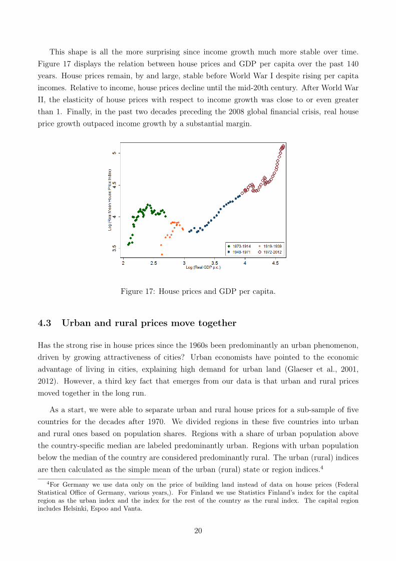
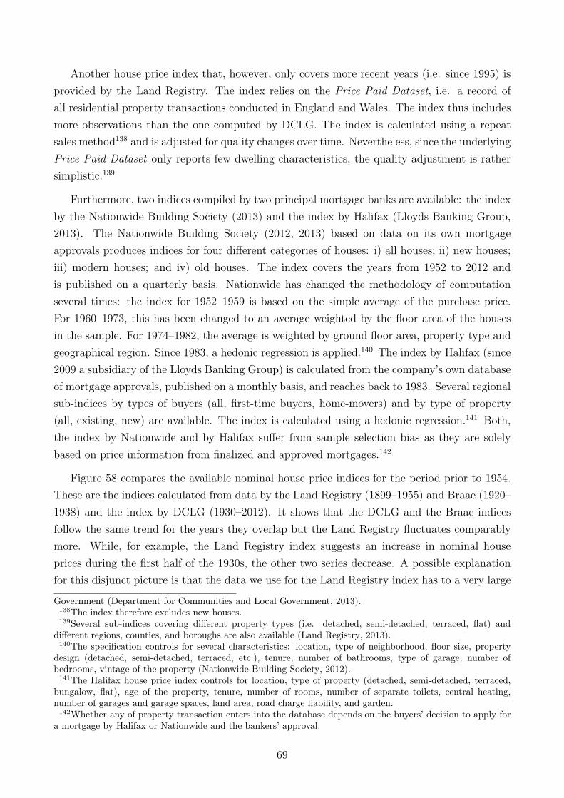
AUS BEL CAN CHE DNK DEU FIN FRA GBR JPN NLD NOR SWE USA Total1870 153 290 568 142 077 1888 048 1554 2156 003 142 036 173 8517 160711880 585 411 1568 257 158 3384 085 2309 2506 016 184 106 588 15009 285461890 1533 453 2854 324 201 4287 190 3328 2783 098 261 156 802 26828 474981900 2129 456 3833 387 291 5168 265 3811 3008 162 277 198 1130 31116 569561910 2805 468 5368 446 345 6121 336 4048 3218 783 319 298 1383 38671 713831920 4177 494 8423 508 433 5755 399 3820 3271 1044 361 329 1487 40692 804681930 4422 513 9106 514 529 5818 513 4240 3263 1457 368 384 1652 40081 832221940 4502 504 9101 522 492 6194 459 4060 3209 1840 331 397 1661 37606 811911950 4446 505 9334 515 482 4982 473 4130 3134 1978 320 447 1652 36014 790141960 4224 463 9526 512 430 5219 532 3900 2956 2048 325 449 1539 35012 771781970 4201 426 9596 501 289 4767 584 3653 1897 2089 315 429 1220 33117 735691980 3946 398 9336 500 294 4575 610 3436 1764 2132 276 424 1201 28800 677731990 3549 351 8688 503 284 4412 585 3432 1658 2025 278 404 1121 24400 639072000 3985 344 7313 449 286 4083 587 3194 1688 2005 280 401 1282 20500 57201Note Dates are approximate Bold denotes peakSources Mitchell (2013) Statistics Canada (various years) Statistics Japan (2012)

Table 3 Length of railway line (in 1000 km) by country

Figure 29 Length of railway network and real freight rates

It is important to note that not only the extension of the global railway network petered outin the first half of the 20th century The dramatic efficiency gains in maritime transportationwere also realized in the late 19th and early 20th century (Mohammed and Williamson 2004)The 19th century revolution in shipping rested on two developments first the fall of ironand steel prices that led to the introduction of metallic hulls second parallel advances inengine technology that led to much improved fuel efficiency (Harley 1988 1980 North 19651958) Between 1870 and 1914 shipping costs fell by about 50 percent relative to the pricesof commodities (Jacks and Pendakur 2010) By contrast as Hummels (2007) has showncommodity-deflated real freight rates barely fell after 1950 Figure 29 exhibits that internationaltransport costs had fallen strongly until the mid-20th century This is likely to have left itsmark on land prices

To analyze how a reduction in transport costs affects the land price we set up a simplemodel with heterogeneous land in the spirit of Ricardo (1817) and von Thuumlnen (1826) Theland rent depends on land location as measured by the distance to the marketplace Falling

35

transportation costs raise the land rent net of transportation costs and lead to an expansionof developed land

Consider a perfectly competitive one-sector economy There is a continuum of firms indexedby i isin [0 1] There is also a continuum of land plots indexed by i isin [0 1] Every firm i isconnected to and owns a piece of land Zi14 The size of each land plot is identical across firmsand normalized to one ie Zi = 1 for all i In equilibrium there are active firms indexed by0 lt i le ilowast as well as inactive firms indexed by ilowast lt i le 1 Active firms develop their land byincurring a fixed cost k and combine (developed) land Zi and labor Li to produce a final outputgood according to Yi = (Li)

α(Zi)1minusα where 0 lt α lt 1 denotes a constant technology parameter

In order to sell their output firms have to transport their products to the marketplace Thisactivity is subject to iceberg transportation costs τi We parametrize the transportation costsby τi = ai where 0 lt a le 1 Normalizing the output price to unity pY = 1 the revenue net oftransportation costs of firm i isin [0 ilowast] is given by Ri = (1minus ai)(Li)α(Zi)

1minusα

The analysis proceeds in two steps The first step focuses on the labor market Individuallabor demand of firm i isin [0 ilowast] for any given wage rate w results from the usual first-order

condition for profit-maximizing labor employment to read as follows Llowasti =[α(1minusai)wlowast(ilowast)

] 11minusα where

we have set Zi = 1 The equilibrium wage rate wlowast(ilowast) is determined by the labor marketclearing condition

int ilowast0Li(w)di = LS where LS denotes exogenous labor supply Notice that

the equilibrium wage rate wlowast(ilowast) increases with the number of active firms ilowast The amountof labor employed by any firm i isin [0 ilowast] in general equilibrium declines as more firms becomeeconomically active or equivalently as more pieces of land are being used economically Thesecond step focuses on the land market Let vZi (τ) denote the land return which may bethought of as residual income accruing to the land owner ie vZi = partR

partZi= (1minusai)(1minusα)(Li)

αThe price pZi of land plot i isin [0 ilowast] is given by the present value of the infinite stream of landreturns ie pZi =

intinfintvZi (τ)eminusr(τminust)dτ Given that vZi is constant in equilibrium the land price

may be expressed as pZi = vZi r where r denotes the constant real interest rate A specificland plot i is being developed if the land price exceeds the development costs ie pZi ge kTherefore the number of developed land plots in equilibrium ilowast equal to the number of activefirms is determined by the following condition

(1minus ailowast)(1minus α)(Llowastilowast)α

r= k (7)

where Llowastilowast is equilibrium labor demand of the marginal firm i = ilowast

What are the effects of radical innovations in the transportation sector like those thatoccurred in the late 19th and early 20th century with respect to land supply The decline in

14Whether firms own a piece of land and reap land return (residual income) or rent the required land fromlandowners by paying a rental rate is not critical with respect to the implications With regard to the landprice both institutional arrangements are equivalent

36

transportation costs enlarged the present value of land returns net of transportation costs forany land plot i Equation 7 then implies that the number of developed land plots rises Inother words the drop in transportation costs triggers an expansion of economically used landFigure 30 illustrates this reasoning The dashed horizontal line shows the constant developmentcosts k while the two downward sloping curves display the value of developed land pZi = vZi r

for alternative values of a15 Now as a falls the curve pZi = vZi r shifts outwards such that ilowast

increases as displayed in Figure 30 The intermediate result therefore is that a reduction intransportation costs unequivocally increases the supply of economically used land

Figure 30 Land supply in response to reduction in transportation costs

How does an increase in land supply triggered by a reduction in transport costs affect theaggregate land price defined as pZ = 1

ilowast

int ilowast0pZi di The combination of reduced transportation

costs and enhanced land supply unfolds three distinct mechanisms with respect to the aggregateland price pZ which can be summarized as follows (for details see Appendix A1)

1 Complementary-factor effect Additional land is developed and employed in output pro-duction Every piece of land is combined with a lower amount of labor This effectdepresses the average land price16

2 Composition effect More distant and therefore less profitable pieces of land are beingdeveloped and used economically This effect also reduces the average land price

15These curves are downward sloping for two reasons First land plots are located further away from themarketplace as i increases which implies higher transportation costs τi = ai Second as i increases the numberof firms - hence aggregate labor demand - goes up such that each piece of land is combined with a lower amountof labor

16There would be an additional effect in multi-sector models As output of the land intensive sector increasesthe goodsrsquo price falls and the competitive land return should decline further

37

3 Revaluation effect Already developed pieces of land become more valuable because thecompetitive land return net of transportation costs vZi increases This effect increases theaverage land price

The complementary-factor effect and the composition effect reduce the land price and thiscan dominate the revaluation effect such that the aggregate land price pZ declines as a falls Ina growing economy the competitive land return can be expected to increase over time becauseland is in fixed supply This drives up land prices But if profit-maximizing firms endogenouslydetermine the overall land use a substantial decline in transportation costs triggers the devel-opment of additional land plots As a result land may effectively not represent a fixed factorfor an extended period and the land price may remain constant or even fall despite continuouseconomic growth

In our view the interaction of transport cost declines and economic growth provides anovel and powerful explanation for the observed path of long-run land prices The large-scale construction of the railway system during the 19th century and early 20th resulted ina substantial decline in transportation costs and likely suppressed land prices during the pre-World War II period After World War II these effects faded so that economic growth led toan increase in the land price In the next section we will discuss two additional factors thatmay have reinforced this trend higher expenditure shares for housing services and growingrestrictions on land use (Glaeser et al 2005a Glaeser and Gyourko 2003)

63 Land prices in the second half of the 20th century

As noted above the trajectory of land prices in the second half of the 20th century is notas puzzling from the perspective of a standard neoclassical model With continuous economicgrowth the value of land could be expected to grow However two additional factors mighthave contributed to an even starker increase of land prices

First empirical data show that the mean housing expenditure share remained nearly con-stant in the pre-World War II period (average annual growth rate 006 percent) whereasit grew by an average annual growth rate of 11 percent after World War II17 However theincrease in expenditure shares is not uniform across countries as Table 4 demonstrates Forinstance the expenditure share remained largely constant in the United States As a resultthe unweighted mean expenditure share shown in Figure 31 may be biased upwards

How did the rising housing expenditure share after World War II impact the evolution ofland prices To answer this question we set up a simple two-sector model with housing and

17The empirical findings on the (long-run) income elasticity of the demand for housing services is howeverinconclusive For instance Fernandez-Kranz and Hon (2006) review the literature and report values that rangebetween 05 percent and 28 percent

38

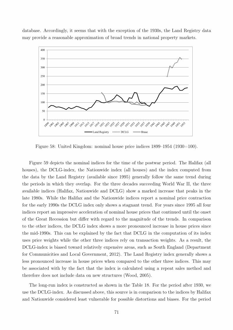
AUS BEL CAN CHE DEU DNK FIN FRA GBR ITA JPN NLD NOR SWE USA1870 012 014 017 014 0151880 013 014 019 013 0101890 014 013 018 012 0121900 011 014 017 011 019 014 01119131914 008 013 016 017 010 016 014 0141920 007 016 012 009 005 008 0111930 010 019 014 019 014 008 012 018 025 0161940 009 019 023 015 019 013 009 015 018 022 0131950 016 010 010 008 011 016 0111960 011 019 016 013 013 018 011 013 019 0141970 014 020 016 017 017 018 018 015 013 015 021 018 0141980 018 021 015 019 025 019 019 016 013 016 021 018 0141990 020 024 021 020 026 018 020 017 016 018 023 019 0152000 020 023 023 023 023 026 025 023 019 018 023 009 019 021 0152010 023 023 024 024 025 029 027 026 025 023 025 010 021 020 016Note Dates are approximate Sources See Appendix B

Table 4 Share of housing expenditure in GDP

manufacturing production described in Appendix A3 to study the quantitative implicationsof rising expenditure shares The intuition is simple As the production of housing servicesrelies more heavily on land ndash the land cost share in production is higher ndash compared to themanufacturing sector aggregate demand for land rises when the expenditure share for housingservices rises With fixed land supply the land price increases A back-of-the-envelope calcu-lation on the basis of the model yields the following results From the data we observe anaverage increase in the expenditure share during the second half of the 20th century by a factorof about 165 Such an increase translates into an additional 42 percent of price appreciationrelative to a scenario with constant expenditure shares The contribution of rising expenditureshares on the land price is therefore substantial Further details on this exercise can be foundin Appendix A3

Figure 31 Share of residential service expenditure in GDP

39

A second important reason for the steep increase of land prices in the second half of the20th century has been pointed out by Glaeser and Ward (2009) Glaeser et al (2005a) andGlaeser and Gyourko (2003) These studies point to growing restrictions on land supply drivenby changes in the regulatory regime that make large-scale development increasingly difficultMore stringent and widespread land use and building regulation were introduced during thesecond half of the 20th century (MacLaughlin 2012 Glaeser et al 2006) As a result of landuse restrictions on new home construction housing supply could not increase in response torising house prices which limited the supply of new homes (Glaeser et al 2005a Glaeser andGyourko 2003) For urban areas in the northeastern US for example Glaeser and Ward(2009) and Glaeser et al (2005b) show that regulations substantially reduced the number ofnew construction permits In the case of the Greater Boston area the total number buildingpermits in the 2000s stood at less than 50 percent of its 1960s level (Glaeser and Ward 2009)These studies further argue that there is a strong relation between house prices and land-useregulation They estimate that in the mid-2000s house prices might have been between 23 (inthe case of Boston) and 50 percent (in the case of Manhattan) lower if regulation had not greatlystagnated new permits (Glaeser et al 2006 2005b) In the US the impact of regulation mayalso explain some of the house price dispersion across American housing markets (Glaeser et al2005a) Similar effects have been documented for other countries such as the UK (Cheshireand Hilber 2008)

To summarize the rise of residential land prices in the second half of the 20th centuryconstitutes much less of a puzzle than their stability in the preceding eight decades Whenthe effects of the transport revolution faded land increasingly became a fixed factor Twoadditional factors are likely to have pushed up land prices even more rising expendituresshares for housing services and growing restrictions on land use

7 Conclusion

In The Wizard of Oz Dorothyrsquos house is transported by a tornado to a strange new plot ofland The story illuminates the fact that a home consists of both the structure of the houseand the underlying land The findings of our study illustrate that it is in fact the price of landthat has been the most significant element for long-run trends in home prices

We show that after a long period of stagnation from 1870 to the mid-20th century houseprices rose strongly in real terms during the second half of the 20th century albeit with consid-erable cross-country heterogeneity These patterns in the data cannot be explained with qualityimprovements or composition shifts in the index Moreover urban and rural house prices haverisen in lockstep in recent decades and farmland prices have also increased

The decomposition of house prices into the replacement cost of the structure and land

40

prices reveals that land prices have been the driving force for the observed trends Residentialland prices have remained constant for almost the first hundred years of modern economicgrowth from the late 19th century until the post-World War II decades but increased stronglythereafter in most countries Stated differently explanations for the long-run trajectory ofhouse prices must be mapped onto the underlying land price dynamics

In this paper we presented two explanations for the trajectory of land prices in moderneconomic history The two explanations complement each other but they are not exclusiveFirst we demonstrated how the transport revolution in the late 19th and early 20th century ledto a substantial drop in transport costs which triggered an increase of land supply This declinein transport costs petered out in the second half of the 20th century so that land increasinglybehaved like a fixed factor Second we revealed evidence that expenditure for housing servicesgrew faster than income after World War II In other words housing appears to behave like asuperior good

In our view the combination of both trends helps explain the cross-country trajectory ofland prices in the 19th and 20th century Additional explanations focusing for instance ongrowing government interventions in the housing market aimed at expanding home ownershipor the easing of financial frictions would be complementary as these factors would show up in arising expenditure share Moreover additional explanations will have to align with the stylizedfacts presented here in particular with the prominent increase of the price of land in the secondhalf of the 20th century and the comparatively minor role of changes in the replacement valueof the structure

Research interest in housing markets has surged in the wake of the global financial crisisYet despite its importance for the discipline of macroeconomics the study of housing mar-ket dynamics was hampered by the lack of comparable long-run and cross-country data fromeconomic history Our study closes this gap We hope that with the data presented in thisstudy new avenues for empirical and theoretical research on housing market dynamics andtheir interactions with the macroeconomy will become possible

41

References

Abelson P and D Chung (2004) ldquoHousing Prices in Australia 1970 to 2003rdquo MacquarieUniversity Economics Research Papers 92004

Abildgren K (2006) ldquoMonetary Trends and Business Cycles in Denmark 1875ndash2005rdquo Dan-marks Nationalbank Working Papers 432006

Adam K and M Woodford (2013) ldquoHousing Prices and Robustly Optimal MonetaryPolicyrdquo mimeo

Association of German Municipal Statisticians (various years) Statistisches JahrbuchDeutscher Staumldte Statistisches Jahrbuch Deutscher Gemeinden Association of GermanMunicipal Statisticians

Australian Bureau of Statistics (2013) ldquoHouse Price Indexes Eight CapitalCitiesrdquo httpwwwabsgovauAUSSTATSabsnsfDetailsPage64160Mar202013

OpenDocument

Bailey M J R F Muth and H O Nourse (1963) ldquoA Regression Method for RealEstate Price Index Constructionrdquo Journal of the American Statistical Association 58 933ndash942

Bank for International Settlements (2013) ldquoProperty Price Statisticsrdquo httpwwwbisorgstatisticspphtm

Bank of Japan (1966) Hundred Year Statistics of the Japanese Economy Tokyo Bank ofJapan

mdashmdashmdash (1986) Bank of Japan The First Hundred Years Appendices Tokyo Bank of Japan

Barro R J (2006) ldquoRare Disasters and Asset Markets in the Twentieth Centuryrdquo TheQuarterly Journal of Economics 121 823ndash866

Belgian Association of Surveyors (2013) ldquoABEX Construction Cost Indexrdquo http

wwwabexbemodulesicontentindexphppage=13

Bohlin J (2014) ldquoA Price Index for Residential Property in Goumlteborg 1875ndash2010rdquo in His-torical Monetary and Financial Statistics for Sweden House Prices Stock Returns NationalAccounts and the Riksbank Balance Sheet 1620ndash2012 ed by R Edvinsson T Jacobsenand D Waldenstroumlm Stockholm Ekerlids vol 2

Bordo M D and J Landon-Lane (2013) ldquoWhat Explains House Price Booms Historyand Empirical Evidencerdquo NBER Working Paper 19584

42

Bourassa S C M Hoesli D Scognamiglio and S Zhang (2011) ldquoLand Leverageand House Pricesrdquo Regional Science and Urban Economics 41 134ndash144

Brunsman H G and D Lowery (1943) ldquoFacts from the 1940 Census of Housingrdquo Journalof Land amp Public Utility Economics 19 89ndash93

Butlin N G (1964) Investment in Australian Economic Development 1861ndash1900 Cam-bridge Cambridge University Press

Canadian Real Estate Association (1981) Annual Report 1981 Ottawa Canadian RealEstate Association

Capozza D R and R W Helsley (1989) ldquoThe Fundamentals of Land Prices and UrbanGrowthrdquo Journal of Urban Economics 26 295ndash306

Case B H O Pollakowski and S M Wachter (1991) ldquoOn Choosing BetweenHouse Price Index Methodologiesrdquo American Real Estate and Urban Economics AssociationJournal 19 286ndash307

Case B and J M Quigley (1991) ldquoThe Dynamics of Real Estate Pricesrdquo Review ofEconomics and Statistics 22 50ndash58

Case B and S Wachter (2005) ldquoResidential Real Estate Price Indices as Financial Sound-ness Indicators Methodological Issuesrdquo in Real Estate Indicators and Financial StabilityBasel Bank for International Settlements no 21 in BIS Papers 197ndash211

Case K E (2007) ldquoThe Value of Land in the United Statesrdquo in Land Policies and theirOutcomes ed by G K Ingram and Y-H Hong Cambridge MA Lincoln Institute of LandPolicy

Case K E and J M Quigley (2008) ldquoHow Housing Booms Unwind Income EffectsWealth Effects and Feedbacks through Financial Marketsrdquo European Journal of HousingPolicy 8 161ndash179

Case K E and R J Shiller (1987) ldquoPrices of Single-Family Homes Since 1970 NewIndexes for Four Citiesrdquo New England Economic Review SeptOct 45ndash56

Centre for Urban Economics and Real Estate University of British

Columbia (2013) ldquoCanadian Cities Housing and Real Estate Datardquo http

wwwsauderubccaFacultyResearch_CentresCentre_for_Urban_Economics_

and_Real_EstateCanadian_Cities_Housing_and_Real_Estate_Data

Cheshire P C and C A Hilber (2008) ldquoOffice Space Supply Restrictions in BritainThe Political Economy of Market Revengerdquo The Economic Journal 118 F185ndashF221

43

Conseil General de lrsquoEnvironnement et du Developpement Durable (2013)ldquoLong Run Data Series 1800ndash2010rdquo httpwwwcgedddeveloppement-durablegouv

frrubriquephp3id_rubrique=137

Davis M A and J Heathcote (2005) ldquoHousing and the Business Cyclerdquo InternationalEconomic Review 46 751ndash784

mdashmdashmdash (2007) ldquoThe Price and Quantity of Residential Land in the United Statesrdquo Journal ofMonetary Economics 54 2595ndash2620 data located at Land and Property Values in the USLincoln Institute of Land Policy httpwwwlincolninsteduresources

Davis M A and M G Palumbo (2007) ldquoThe Price of Residential Land in Large USCitiesrdquo Journal of Urban Economics 63 352ndash384

De Bruyne J-P (1956) ldquoLrsquoEvolution des Prix des Immeubles Urbains de lrsquoAgglomerationBruxelloise de 1878 a 1952rdquo Bulletin de lrsquoInstitut de Recherches Economiques et Sociales 2257ndash93

Del Negro M and C Otrok (2007) ldquo99 Luftballons Monetary Policy and the HousePrice Boom across US Statesrdquo Journal of Monetary Economics 54 1962ndash1985

Department for Communities and Local Government (2013)ldquoHouse prices from 1920 annual house price inflation United Kingdomfrom 1970rdquo httpswwwgovukgovernmentstatistical-data-sets

live-tables-on-housing-market-and-house-prices

Deutsches Volksheimstaumlttenwerk (1959) Handhabung des Preisstops Grundstuumlck-spreisentwicklung und Anwendung des Baulandbeschaffungsgesetzes vol 14 of Wis-senschaftliche Untersuchungen und Vortraumlge Cologne Deutsches Volksheimstaumlttenwerk

Eichholtz P M (1994) ldquoA Long-Run House Price Index The Herengracht Index 1628ndash1973rdquo Real Estate Economics 25 175ndash192

Eitrheim O and S K Erlandsen (2004) ldquoHouse Price Indices for Norway 1819ndash2003rdquoin Historical Monetary Statistics for Norway 1819ndash2003 ed by O Eitrheim J T Klovlandand J F Ovigstad Oslo Norges Bank no 35 in Norges Bank Skriftserie OccasionalPapers

European Commission (2013) ldquoHandbook on Residential Property Price Indices (RPPIs)rdquoeurostat Methodologies and Working papers

Federal Housing Finance Agency (2013) ldquoHouse Price Indexesrdquo httpwwwfhfa

govDefaultaspxPage=87

44

Federal Statistical Office of Germany (various years) Kaufwerte fuumlr Bauland Fach-serie 17 Reihe 5 Wiesbaden Federal Statistical Office of Germany

Feinstein C H and S Pollard (1988) Studies in Capital Formation in the UnitedKingdom 1750ndash1920 Oxford Clarendon Press

Fernandez-Kranz D and M T Hon (2006) ldquoA Cross-Section Analysis of the IncomeElasticity of Housing Demand in Spain Is There a Real Estate Bubblerdquo Journal of RealEstate Financial Economics 32 449mdash470

Firestone O J (1951) Residential Real Estate in Canada Toronto University of TorontoPress

Fishback P V and T Kollmann (2012) ldquoNew Multi-City Estimates of the Changes inHome Values 1920-1940rdquo NBER Working Paper 18272

Fishback P V J Rose and K Snowden (2013) Well Worth Saving How the NewDeal Safeguarded Home Ownership Chicago University of Chicago Press

Fleming M (1966) ldquoThe Long-Term Mesurement of Construction Costs in the United King-domrdquo Journal of the Royal Statistical Society 129 534ndash556

Francke M and A van de Minne (2013) ldquoLand Structure and Depreciationrdquo ResearchPaper Universiteit van Amsterdam

Geltner D and D Ling (2006) ldquoConsiderations in the Design and Construction of Invest-ment Real Estate Research Indicesrdquo Journal of Real Estate Research 28 411ndash444

General Register Office (1951) Census 1951 England and Wales Preliminary ReportLondon HMSO

Glaeser E L J D Gottlieb and K Tobio (2012) ldquoHousing Booms and City CentersrdquoAmerican Economic Review 102 127ndash133

Glaeser E L and J Gyourko (2003) ldquoThe Impact of Building Restrictions on HousingAffordabilityrdquo FRBNY Economic Policy Review 9 21ndash39

Glaeser E L J Gyourko and R Saks (2005a) ldquoWhy Have Housing Prices Gone UprdquoAmerican Economic Review 95 329ndash333

mdashmdashmdash (2005b) ldquoWhy is Manhattan So Expensive Regulation and the Rise in House PricesrdquoJournal of Law and Economics 48 331ndash370

Glaeser E L and J E Kohlhase (2004) ldquoCities Regions and the Decline of TransportCostsrdquo Papers in Regional Science 83 197ndash228

45

Glaeser E L J Kolko and A Saiz (2001) ldquoConsumer Cityrdquo Journal of EconomicGeography 1 27ndash50

Glaeser E L J Schuetz and B A Ward (2006) Regulation and the Rise of Hous-ing Prices in Greater Boston Boston MA Pioneer Institute for Public Policy ResearchCambridge MA Rappaport Institute for Greater Boston

Glaeser E L and B A Ward (2009) ldquoThe Causes and Consequences of Land UseRegulation Evidence from Greater Bostonrdquo Journal of Urban Economics 65 265ndash278

Goodhart C and B Hofmann (2008) ldquoHouse Prices Money Credit And the Macroe-conomyrdquo Oxford Review of Economic Policy 24 180ndash205

Grebler L D M Blank and L Winnick (1956) Capital Formation in ResidentialReal Estate Trends and Prospects Princeton Princeton University Press

Gyourko J C Mayer and T Sinai (2006) ldquoSuperstar Citiesrdquo American EconomicJournal 5 167ndash199

Harley C (1980) ldquoTransportation the World Wheat Trade and the Kuznets Cycle 1850ndash1913rdquo Explorations in Economic History 17 218ndash250

mdashmdashmdash (1988) ldquoOcean Freight Rates and Productivity 1740ndash1913 The Primacy of MechanicalInvention Reaffirmedrdquo Journal of Economic History 48 851ndash875

Hendershott P H and T G Thibodeau (1990) ldquoThe Relationship between Medianand Constant Quality House Prices Implications for Setting FHA Loan Limitsrdquo Real EstateEconomics 18 323ndash334

Hornstein A (2009a) ldquoNote on a Model of Housing with Collateral Constraintsrdquo FRBRichmond Working Paper 09-3

mdashmdashmdash (2009b) ldquoProblems for a Fundamental Theory of House Pricesrdquo FRB Richmond Eco-nomic Quarterly 95 1ndash24

Hummels D (2007) ldquoTransportation Costs and International Trade in the Second Era ofGlobalizationrdquo Journal of Economic Perspectives 21 131ndash154

Jacks D S and K Pendakur (2010) ldquoGlobal Trade and the Maritime Transport Revo-lutionrdquo The Review of Economics and Statistics 92 745ndash755

Janssens P and P de Wael (2005) 50 Jaar Belgische Vastgoedmarkt Waar GeschiedenisTot Toekomst Vergroeit Brussels Roularta Books

Jordagrave O M Schularick and A M Taylor (2014) ldquoBetting the Houserdquo mimeo

46

Land Registry (2013) ldquoHouse Price Indexrdquo httpwwwlandregistrygovukpublic

house-prices-and-sales

Leamer E E (2007) ldquoHousing IS the Business Cyclerdquo in Proceedings - Economic PolicySymposium - Jackson Hole ed by F K City 149ndash233

Mack A and E Martiacutenez-Garciacutea (2012) ldquoA Cross-Country Quarterly Database of RealHouse Prices A Methodological Noterdquo FRB Dallas Globalization and Monetary Policy In-stitute Working Paper 99

MacLaughlin R B (2012) ldquoLand Use Regulation Where Have We Been Where Are WeGoingrdquo Cities 29 S50ndashS55

Maiwald K (1954) ldquoAn Index of Building Costs in the United Kingdom 1845ndash1938rdquo TheEconomic History Review 7 187ndash203

Matti W (1963) ldquoHamburger Grundeigentumswechsel und Bauland 1903ndash1907 und 1955ndash1962rdquo Hamburg in Zahlen Monatsschrift des Statistischen Landesamtes der Freien undHansestadt Hamburg

Mian A and A Sufi (2014) ldquoHouse Price Gains and US Household Spending from 2002to 2006rdquo mimeo

Mitchell B (2013) ldquoInternational Historical Statistics 1750ndash2010 [Online]rdquo httpwwwpalgraveconnectcompcdoifinder1010579781137305688

Mohammed S I and J G Williamson (2004) ldquoFreight Rates And Productivity GainsIn British Tramp Shipping 1869-1950rdquo Explorations in Economic History 41 172ndash203

National Institute of Statistics and Economic Studies (2012) ldquoComptesdu Logement 2011 Tableaux de Donnees 2011 et Series Chronologiques 1984ndash2011rdquo httpwwwstatistiquesdeveloppement-durablegouvfrpublicationsp

referencescomptes-logement-2011-premiers-resultats-2012html

Nichols D A (1970) ldquoLand and Economic Growthrdquo American Economic Review 60 332ndash340

Norges Eiendomsmeglerforbund (2012) ldquoBoligprissstatistikkrdquo httpwwwnefno

xppubtoppboligprisstatistikk

North D (1958) ldquoOcean Freight Rates and Economic Development 1750ndash1913rdquo Journal ofEconomic History 18 537ndash555

mdashmdashmdash (1965) ldquoThe Role of Transportation in the Economic Development of North Americardquoin Les Grandes voies maritimes dans le monde XV-XIX siecles ed by International Commit-tee of Historical Sciences Commission internationale drsquohistoire maritime Paris SEVPEN

47

OECD (2014) OECDStat Paris OECD

Piketty T (2014) Capital in the Twenty-First Century Cambridge Harvard UniversityPress

Piketty T and G Zucman (2014) ldquoCapital Is Back Wealth-to-Income Ratios in RichCountries 1700ndash2010rdquo Quarterly Journal of Economics 129

Ricardo D (1817) Principles of Political Economy and Taxation

Schularick M and A M Taylor (2012) ldquoCredit Booms Gone Bust Monetary PolicyLeverage Cycles and Financial Crises 1870ndash2008rdquo American Economic Review 102 1029ndash1061

Shiller R J (1993) ldquoMeasuring Asset Values for Cash Settlement in Derivative MarketsHedonic Repeated Measures Indices and Perpetual Futuresrdquo Journal of Finance 48 911ndash931

mdashmdashmdash (2009) Irrational Excuberance New York Broadway Books 2nd revised and updateded

Silver M (2012) ldquoWhy House Price Indexes Differ Measurement and Analysisrdquo IMF Work-ing Paper 12125

Soumlderberg J S Bloumlndal and R Edvinsson (2014) ldquoA Price Index for Residen-tial Property in Stockholm 1875ndash2012rdquo in Historical Monetary and Financial Statistics forSweden House Prices Stock Returns National Accounts and the Riksbank Balance Sheet1620ndash2012 ed by R Edvinsson T Jacobsen and D Waldenstroumlm Stockholm Ekerlidsvol 2

Stapledon N (2007) ldquoLong Term Housing Prices in Australia and Some Economic Perspec-tivesrdquo PhD thesis University of New South Wales Sydney

mdashmdashmdash (2012a) ldquoHistorical Housing-Related Statistics for Australia 1881ndash2011 ndash A Short NoterdquoUNSW Australian School of Business Research Paper 522012

mdashmdashmdash (2012b) ldquoTrends and Cycles in Sydney and Melbourne House Prices from 1880 to 2011rdquoAustralian Economic History Review 52 203ndash217

Statistical Office of the City of Helsinki (various years) Helsinki Statistical Year-book Helsinki Helsingin Kaupungin Tilastokonttorin

Statistics Belgium (2013) ldquoBouw En Industrie - Verkoop Van Onroerende Goed-eren 1986ndash2012rdquo httpstatbelfgovbenlmodulespublicationsstatistiques

economiedownloadsbouw_en_industrie_verkoop_onroerende_goederenjsp

48

Statistics Berlin (various years) Statistisches Jahrbuch der Stadt Berlin Berlin StatisticsBerlin

Statistics Canada (various years) Canada Year Book Ottawa

Statistics Finland (2011) ldquoPrices of Dwellings in Housing Companiesrdquo http

wwwstatfitilashi201102ashi_2011_02_2011-07-29_laa_001_enhtml2

Methodologicaldescription

Statistics Japan (2012) ldquoHistorical Statistics of Japanrdquo httpwwwstatgojp

englishdatachoukiindexhtm

mdashmdashmdash (2013) ldquoJapan Statistical Yearbook 2013rdquo httpwwwstatgojpenglishdata

nenkanindexhtm

Statistics Netherlands (2013) ldquoPrijzen Bestaande Koopwoningenrdquo httpwwwcbsnlnl-NLmenuthemasprijzencijfersdefaulthtm

Summerhill W (2006) ldquoThe Development of Infrastructurerdquo in The Cambridge EconomicHistory of Latin America ed by V Bulmer-Thomas J H Coatsworth and R C CondeCambridge MA Cambridge University Press vol 2 293ndash326

Swiss Federal Statistical Office (2013) ldquoStadt Zuumlrich Handaumlnderungen von Grund-stuumlcken nach Art des Kaufs 1899ndash1990rdquo httpwwwbfsadminchbfsportalde

indexinfotheklexikonlex2Document81325xls

Taylor G R (1951) The Transportation Revolution 1815ndash1860 vol 4 of Economic Historyof the United States ME Sharpe

United Nations (2014) On-line Data Urban and Rural Population New York UnitedNations

US Bureau of the Census (1975) Historical Statistics of the United States ColonialTimes to 1970 Washington US Dept of Commerce Bureau of the Census

von Thuumlnen J H (1826) Der isolierte Staat in Beziehung auf Landwirtschaft und Nation-aloumlkonomie

Wickens D L (1937) Financial Survey of Urban Housing Statistics on Financial Aspectsof Urban Housing Washington US Department of Commerce

Williamson J and K OrsquoRourke (1999) Globalization and History Cambridge MA MITPress

Wuumlest and Partner (2012) Immo-Monitoring 2012-1

49

No Price Like HomeGlobal House Prices 1870ndash2012

Appendix

1

Contents

Contents 2

A Supplementary material 3

A1 Land heterogeneity and transportation costs 3

A2 A brief review of the theoretical literature 4

A3 Housing expenditure share 5

A4 Figures and tables 7

B Data appendix 8

B1 Description of the methodological approach 8

B2 Australia 10

B3 Belgium 18

B4 Canada 23

B5 Denmark 29

B6 Finland 33

B7 France 37

B8 Germany 41

B9 Japan 48

B10 The Netherlands 53

B11 Norway 56

B12 Sweden 60

B13 Switzerland 63

B14 United Kingdom 67

B15 United States 74

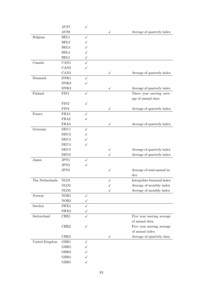
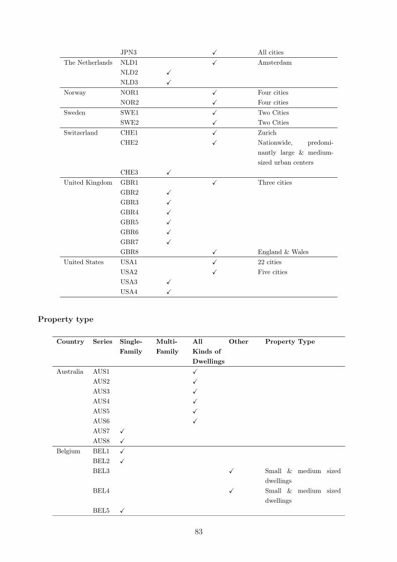
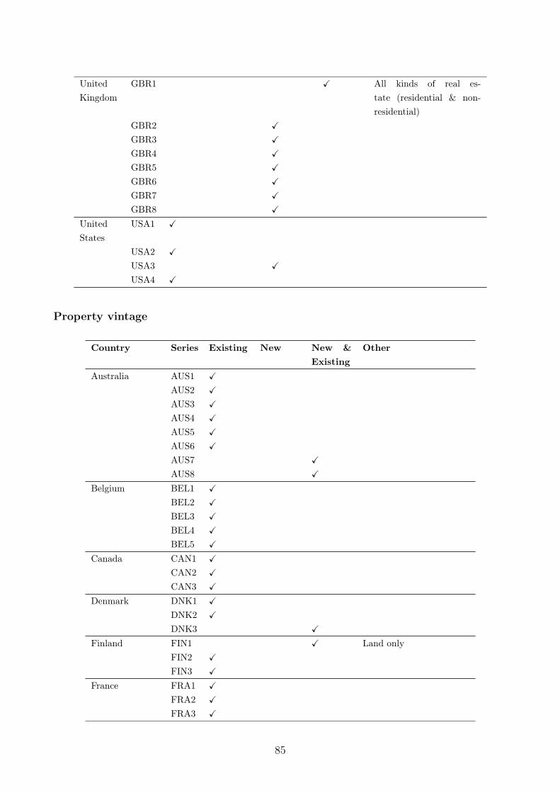
B16 Summary of house price series 80

References 90

2

Appendix

A Supplementary material

A1 Land heterogeneity and transportation costs

This brief section demonstrates how to solve the land price model in the spirit of Ricardo andvon Thuumlnen presented in section 62 for the land price The notation is as explained in themain text We start with the labor market equilibrium for a given number of active firms iFrom the first-order condition for optimal labor demand w = (1 ai)crarr(Li)crarr1 (recall Zi = 1)the individual labor demand schedule reads

Li(w) =

crarr(1 ai)

w

11crarr

(8)

The equilibrium wage rate w results from the labor market clearing condition which equatesaggregate labor demand

R i

0 Li(w)di and aggregate labor supply LS Noting Equation 8 onegets

Z i

0

crarr(1 ai)

w

11crarr

di = Ls (9)

where i denotes the number of active firms in equilibrium which is treated as unknown at thisstage Determining the definite integral on the LHS of Equation 9 and solving with respect tow gives w = w(i a) At this stage individual labor demand in equilibrium L

i (w) can be

determined for any given i

Next we turn to the land market The competitive land return is given by the marginalproduct of land in output production net of transportation costs ie

vZi =(1 ai)Yi

Zi

= (1 ai)(1 crarr)(Li)crarr (10)

The price pZi of land plot i 2 [0 i] is given by the present value of the infinite stream of landreturns ie pZi =

R1t

vZi ()er(t)d Given that vZi is constant in equilibrium the land price

may be expressed as pZi = vZi r A specific land plot i is being developed if the land priceexceeds the development costs ie pZi k Therefore the number of developed land plots inequilibrium i equal to the number of active firms is determined by the following condition

(1 ai)(1 crarr) [Li(w

)]crarr

r= k (11)

where Li(w

) is equilibrium labor demand of the marginal firm i = i The preceding equationnoting w = w(i a) determines the number of active firms as a function of a ie i = i(a)

3

The aggregate land price is defined as pZ = 1i

R i

0 pZi di Noting pZi = vZi r and vZi =

(1 ai)(1 crarr)(Li)crarr pZi may be expressed as follows

pZ =1

i(a)

Z(1)z|i(a)

0

(1

(2)z|a i)(1 crarr)[L

i (w(i(

(3)z|a )))]crarr

rdi (12)

where (1) indicates the composition effect (2) the revaluation effect and (3) the comple-mentary factor effect respectively The RHS of the preceding equation indicates how a changein a influences the equilibrium land price

A2 A brief review of the theoretical literature

This section provides a brief review of the theoretical literature on the housing market Davisand Heathcote (2005) set up a multi-sector growth model with housing production The focusis however not on the evolution of aggregate house prices but on stylized business cycle factsassociated with residential and non-residential investments Hornstein (2009ba) followingDavis and Heathcote sets up a general equilibrium model that captures a housing market Thefocus is on the surge in house prices in the US between 1975 and 2005 The main drivingforce is the increasing relative scarcity of land as measured by the difference between thegrowth rate of per capita income and the growth rate at which new land becomes availableDavis and Heathcote (2007 2597) have found based on empirical work for the US over1975 to 2005 that both trend growth in house prices and cyclical house price fluctuations areprimarily attributable to changes in the price of residential land and not to changes in the priceof structure Hornstein argues that this model has the clear potential to account for the trendin prices of new houses although it cannot account for the differential price trends in the marketfor new and existing houses Li and Zeng (2010) employ a two-sector neoclassical growth modelwith housing to explain a rising real house price driven by a comparably low technical progressin the construction sector Poterba (1984) employs a dynamic model of the housing sector tostudy how inflation affects the real house price and the size of the housing stock He argues thatpersistent high inflation rates reduces homeownersrsquo user cost and may lead to an increase inhouse prices and the housing stock Glaeser et al (2005a) show that focusing on the US sincethe 1970s changes in the housing-supply regulations caused house prices to increase Glaeserand Gottlieb (2009 44) stress that urbanization induced by agglomeration economies andinelastic housing supply in cities pushes the aggregate housing prices upwards

4

A3 Housing expenditure share

Consider a perfectly competitive and static economy with two sectors In the manufacturingsector labor L is combined with land ZM to produce consumption goods M Moreover realestate development firms combine structures X and land ZH to produce residential servicesOne house generates one unit of housing services As the model describes a static economythere is no stock of houses that may accumulate over time The house price and the price forhousing services therefore coincide The sectoral production functions read as follows

M = (L)1crarr ZMcrarr

(13)

H = (X)1 ZH

(14)

where 0 lt crarr lt 1 denote constant technology parameters Only the intersectoral allocationof land is endogenous whereas L and X are fixed18 Aggregate income is given by PY =

pMM + pHH where P = 1 denotes the price level pM the (real) price of the manufacturinggood and pH the (real) price of residential services Let 0 lt lt 1 denote the share of incomedevoted to housing services ie = pHH

Y Equilibrium in the market for residential services is

then described by19

pHH = Y (15)

Total land supply is fixed and normalized to one The land constraint reads ZM + ZS = 1The intersectoral land allocation is determined by the equality of the competitive land returnsacross sectors ie

pMcrarrM

ZM= pH

H

ZH (16)

The land return equals the land price in this static model ie pZ = pMcrarr MZM The equi-

librium share of land allocated to the housing sector turns out to read ZH = (crarr)+crarr

Noticethat unsurprisingly the share of land allocated to the housing sector increases with the housingexpenditure share ie ZH

gt 0

What is the consequence of a rising housing expenditure share with respect to the landprice pZ The answer is provided by

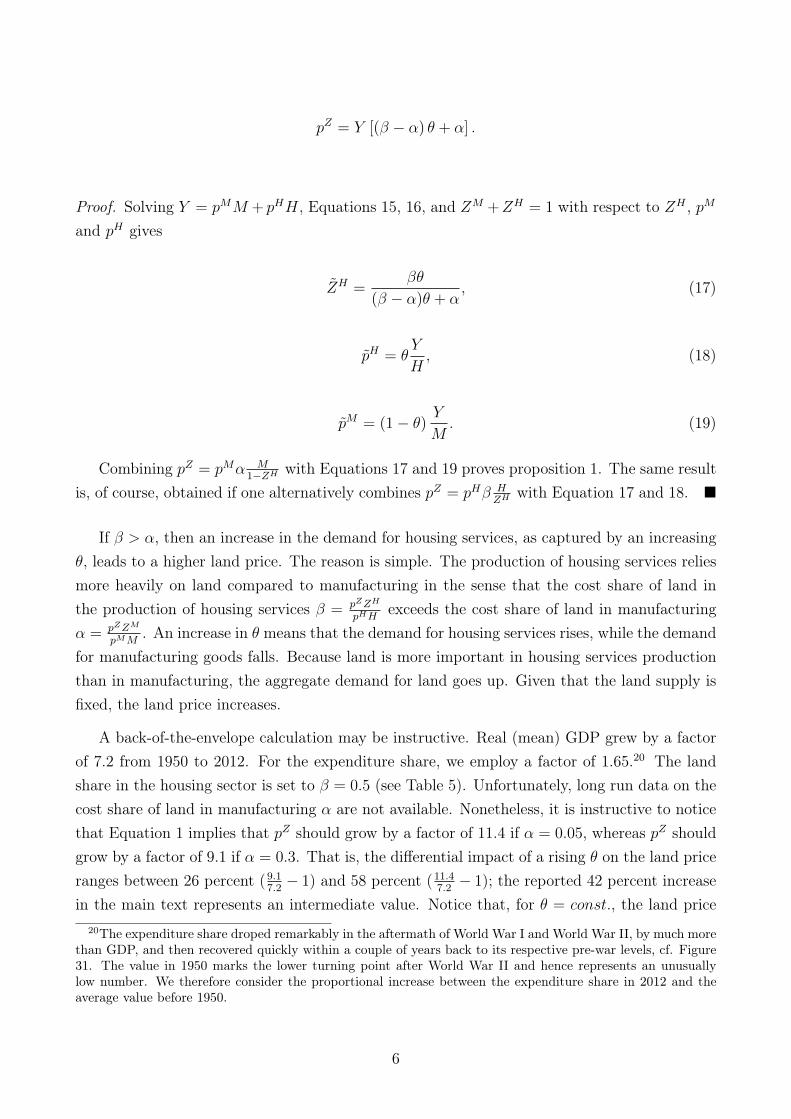
Proposition 1 The equilibrium land price pZ reads as follows18One can easily modify this simplifying assumption without major implications19Due to Walrasrsquo law the market for manufacturing goods clears as well

5

pZ = Y [( crarr) + crarr]

Proof Solving Y = pMM + pHH Equations 15 16 and ZM +ZH = 1 with respect to ZH pM

and pH gives

ZH =

( crarr) + crarr (17)

pH = Y

H (18)

pM = (1 )Y

M (19)

Combining pZ = pMcrarr M1ZH with Equations 17 and 19 proves proposition 1 The same result

is of course obtained if one alternatively combines pZ = pH HZH with Equation 17 and 18

If gt crarr then an increase in the demand for housing services as captured by an increasing leads to a higher land price The reason is simple The production of housing services reliesmore heavily on land compared to manufacturing in the sense that the cost share of land inthe production of housing services = pZZH

pHHexceeds the cost share of land in manufacturing

crarr = pZZM

pMM An increase in means that the demand for housing services rises while the demand

for manufacturing goods falls Because land is more important in housing services productionthan in manufacturing the aggregate demand for land goes up Given that the land supply isfixed the land price increases

A back-of-the-envelope calculation may be instructive Real (mean) GDP grew by a factorof 72 from 1950 to 2012 For the expenditure share we employ a factor of 16520 The landshare in the housing sector is set to = 05 (see Table 5) Unfortunately long run data on thecost share of land in manufacturing crarr are not available Nonetheless it is instructive to noticethat Equation 1 implies that pZ should grow by a factor of 114 if crarr = 005 whereas pZ shouldgrow by a factor of 91 if crarr = 03 That is the differential impact of a rising on the land priceranges between 26 percent (9172 1) and 58 percent (11472 1) the reported 42 percent increasein the main text represents an intermediate value Notice that for = const the land price

20The expenditure share droped remarkably in the aftermath of World War I and World War II by much morethan GDP and then recovered quickly within a couple of years back to its respective pre-war levels cf Figure31 The value in 1950 marks the lower turning point after World War II and hence represents an unusuallylow number We therefore consider the proportional increase between the expenditure share in 2012 and theaverage value before 1950

6

increases by a factor of 72 due to GDP growth Recall also that our imputed land price asdisplayed in Figure 26 grew by a factor of 113

A4 Figures and tables

Figure 32 Imputed land prices - sensitivity analysis

Figure 33 Imputed land prices - individual countries

7

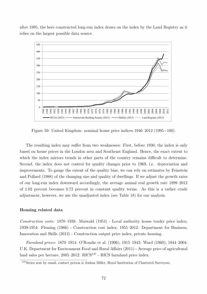
AUS CAN CHE DEU DNK FRA GBR ITA JPN NLD NOR SWE USA18701880 075 013 052 025 074 020 0301890 0401900 054 070 018 051 062 023 040 029 04819131914 043 073 020 052 030 040 028 043 031 0511920 0511930 040 061 017 046 030 023 031 052 034 0491940 054 017 045 019 033 046 033 0431950 049 056 017 028 032 017 025 065 015 0291960 040 052 017 032 030 012 026 085 031 0461970 048 048 025 038 030 015 028 086 038 031 0471980 040 052 048 030 041 011 026 081 038 032 0471990 062 047 036 042 0902000 063 049 032 039 081 0572010 071 053 037 059 077 053Note Dates are approximate Sources See Appendix B

Table 5 Share of land in total housing value

B Data appendix

This data appendix supplements our working paper No Price Like Home Global HousePrices 1870ndash2012 The main purpose of this appendix is to provide an overview about thedata sources we had at our disposal and discuss all relevant details of the sources we finallyused for constructing our long-run house price indices We present residential house priceindices for 14 advanced economies that cover the years 1870 to 2012

A large number of researchers and statisticians offered advice helped in locating data andshared their data sources We wish to thank Paul de Wael Christopher Warisse Willy Biese-mann Guy Lambrechts Els Demuynck and Erik Vloeberghs (Belgium) Debra Conner Gre-gory Klump Marvin McInnis (Canada) Kim Abildgren Finn Oslashstrup and Tina Saaby Hvolboslashl(Denmark) Riitta Hjerppe Kari Levaumlinen Juhani Vaumlaumlnaumlnen and Petri Kettunen (Finland)Jacques Friggit (France) Carl-Ludwig Holtfrerich Petra Hauck Alexander Nuumltzenadel Ul-rich Weber and Nikolaus Wolf (Germany) Alfredo Gigliobianco (Italy) Makoto Kasuya andRyoji Koike (Japan) Alfred Moest (The Netherlands) Roger Bjornstad and Trond AmundSteinset (Norway) Daniel Waldenstroumlm (Sweden) Annika Steiner Robert Weinert Joel FlorisFranz Murbach Iso Schmid and Christoph Enzler (Switzerland) Peter Mayer Neil MonneryJoshua Miller Amanda Bell Colin Beattie and Niels Krieghoff (United Kingdom) JonathanD Rose Kenneth Snowden and Alan M Taylor (United States) Magdalena Korb helped withtranslation

B1 Description of the methodological approach

Data sources

Most countriesrsquo statistical offices or central banks began only recently to collect data on houseprices For the 14 countries covered in our sample data from the early 1970s to the present

8

can be accessed through three principal internationally recognized repositories the databasesmaintained by the Bank for International Settlements (2013) the OECD and the FederalReserve Bank of Dallas (2013) To extend these back to the 19th century we used threeprincipal types of country specific data

First we turn to national official statistical publications such as the Helsinki StatisticalYearbook or the annual publications of the Swiss Federal Statistical office and collectionsof data based on official statistical abstracts Typically such official statistics publicationscontained raw data on the number and value of real estate transactions and in some casesprice indices A second key source are published and unpublished data gathered by legal or taxauthorities (eg the UK Land Registry ) or national real estate associations (eg the CanadianReal Estate Association) Third we can also draw on the previous work of financial historiansand commercial data providers

Selection of house price series

Constructing long-run data series usually involves a good many compromises between the idealand the available data This is also true for each of our 14 house price indices Typicallywe found series for shorter periods and had to splice them to arrive at a long-run indexThe historical data we have at our disposal vary across countries and time with respect tokey characteristics (area covered property type frequency etc) and in the method used forindex construction In choosing the best available country-year-series we follow three guidingprinciples constant quality longitudinal consistency and historical plausibility

We select a primary series that is available up to 2012 refers to existing dwellings andis constructed using a method that reflects the pure price change ie controls for changesin composition and quality When extending the series we concentrate on within-countryconsistency to avoid principal structural breaks that may arise from changes in the marketsegment a country index covers We therefore while aiming to ensure the broadest geographicalcoverage for each of the 14 country indices wherever possible and reasonable maintain thegeographical coverage of the indices Likewise we try to keep the type of house covered constantover time be it single-family houses terraced houses or apartments We examine the historicalplausibility of our long-run indices We heavily draw on country specific economic and socialhistory literature as well as primary sources such as newspaper accounts or contemporarystudies on the housing market to scrutinize the general trends and short-term fluctuations inthe indices Based on extensive historical research we are confident that the indices offer areasonably time-consistent picture of house price developments in each of our 14 countries

9

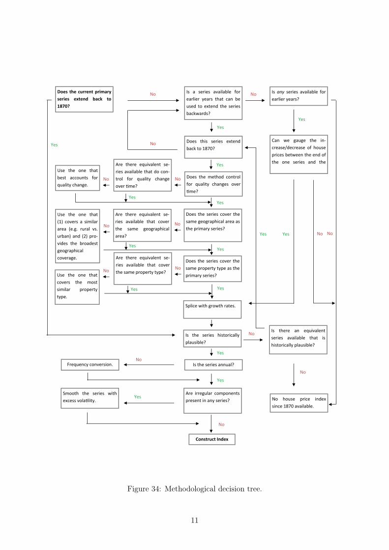
Construct the country indices step by step

The methodological decision tree in Figure 34 describes the steps we follow to construct consis-tent series by combining the available sources for each country in the panel By following thisprocedure we aim to maintain consistency within countries while limiting data distortions Inall cases the primary series does not extend back to 1870 but has to be complemented withother series

Other housing statistics

We complement the house price data with three additional housing related data series prices offarmland construction costs and estimates for the total value of the housing stock For pricesof farmland we again rely on official statistical publications and series constructed by otherresearchers For benchmark data on the total market value of housing and its components(ie structures and land) we turn to the OECD database of national account statistics forthe most recent period (with different starting points depending on the country) We consultthe work of Goldsmith (1981 1985) and also build on more recent contributions such asPiketty and Zucman (2014) (for Australia Canada France Germany Italy Japan the USand UK) and Davis and Heathcote (2007) (for the US) to cover earlier years For dataon construction costs we mostly draw on publications by national statistical offices In somecases we also rely on the work of other scholars such as Stapledon (2012a) Maiwald (1954) andFleming (1966) national associations of builders or surveyors (Belgian Association of Surveyors2013) or journals specializing in the building industry (Engineering News Record 2013) Formacroeconomic and financial variables we rely on the long-run macroeconomic dataset fromSchularick and Taylor (2012) and the update presented in Jordagrave et al (2013)

B2 Australia

House price data

Historical data on house prices in Australia is available for 1870ndash2012

The most comprehensive source for house prices for the Sydney and Melbourne area isStapledon (2012b) His indices cover the years 1880ndash2011 For the sub-period 1880ndash1943 theyare computed from the median asking price for all residential buildings indiscriminate of theircharacteristics and specifics for 1943ndash1949 Stapledon (2012b) estimates a fixed prices21 for1950ndash1970 he uses the median sales price22 For the sub-period 1970ndash1985 Stapledon (2012b)

21Price controls on houses and land were imposed in 1942 and were only removed in 1948 (Stapledon 200723 f)

22The ask price series for residential houses (1880ndash1943) and the sales price series (1948ndash1970) are compiled

10

Does thecurrentprimaryseries extend back to1870

ConstructIndex

Are there equivalent seͲriesavailablethatdoconͲtrol for quality changeoverƟme

Is the series historicallyplausible

IstheseriesannualFrequencyconversion

Are irregular componentspresentinanyseries

Smooth the series withexcessvolaƟlity

YesNo

Yes

No

Is a series available forearlier years that can beused toextend the seriesbackwards

Is any series available forearlieryears

No No

Does this series extendbackto1870

Can we gauge the inͲcreasedecrease of housepricesbetweentheendofthe one series and the

Does themethod controlfor quality changes overƟme

Does the series cover thesamegeographicalareaastheprimaryseries

Splicewithgrowthrates

Yes

No

Is there an equivalentseries available that ishistoricallyplausible

No

NoDoes the series cover thesamepropertytypeastheprimaryseries

No

Yes

Use the one thatbest accounts forqualitychange

Use the one that(1) covers a similararea (eg rural vsurban)and (2)proͲvides the broadestgeographicalcoverage

No

Use the one thatcovers the mostsimilar propertytype

No

No house price indexsince1870available

No

Yes No

Yes

Are there equivalent seͲries available that coverthesamepropertytype

Yes

Are there equivalent seͲries available that coverthe same geographicalarea

Figure 34 Methodological decision tree

11

relies on estimates of median house prices by Abelson and Chung (2004) (see below) for 1986ndash2011 he uses the Australian Bureau of Statistics (2013b) (see below) index for establishedhouses

The median house price series compiled by Abelson and Chung (2004)23 for Sydney andMelbourne are constructed from various data sources for the Sydney series they rely on i) a1991 study by Applied Economics and Travers Morgan which draws on sales price data from theLand Title Offices (for 1970ndash1989) and ii) on sales price data from the Department of Housingie the North South Wales Valuer-General Office (for 1990ndash2003) For the Melbourne seriesthe authors rely on previously unpublished sales price data from the Productivity Commissiondrawing in turn on Valuer-General Office (for 1970ndash1979) and Victorian Valuer-General Officesales price data (for 1980ndash2003)

Besides the Sydney and Melbourne house price indices (see above) Stapledon (2007 64 ff)provides aggregate median price series for detached houses for the six Australian state capitals(Adelaide Brisbane Hobart Melbourne Perth Sydney) for the years 1880ndash2006 As houseprice data is ndash with the exception of Melbourne and Sydney ndash not available for the time priorto 1973 the author uses census data on weekly average rents to estimate rent-to-rent ratios24

The rent-to-rent-ratios are then used to estimate mean and median price data for detachedhouses in the four state capitals (Adelaide Brisbane Hobart Perth) based on the weightedmean price series for SydneyndashMelbourne for the time 1901ndash197325 For the years after 1972Stapledon (2007 234 f) uses the Abelson and Chung (2004) series for the period 1973ndash1985and the Australian Bureau of Statistics (2013b) series for 1986ndash2006 (see below)

In addition to Stapledon (2012b 2007) and Abelson and Chung (2004) four early additionalhouse price data series and indices for Sydney and Melbourne are available i) Abelson (1985)provides an index for Sydney for 1925ndash197026 ii) Neutze (1972) presents house price indicesfor four areas in Sydney (1949ndash1967)27 iii) Butlin (1964) presents data for Melbourne (1861ndash

from weekly property market reports in the Sydney Morning Herald and the Melbourne Age The reports arefor auction sales and private treaty sales

23Abelson and Chung (2004) also present series for Brisbane (1973ndash2003) Adelaide (1971ndash2003) Perth (1970ndash2003) Hobart (1971ndash2003) Darwin (1986ndash2003) and Canberra (1971ndash2003) For details on the data sourcesused for these cities see Abelson and Chung (2004 10)

24The ratios are computed from average weekly rents for detached houses in the four state capitals (numer-ators) and a weighted weekly rent calculated from data for Sydney and Melbourne (denominators) Data isavailable for the years 1911 1921 1933 1947 and 1954

25The same method is applied to extend the series backwards ie to the period 1880ndash1900 Each cityrsquos shareof houses is applied for weighting

26Abelson (1985) collects sales and valuation prices from the NSW Valuer-Generalrsquos records for about 200residential lots in each of the 23 local government areas He calculates a mean a median and a repeat valuationindex

27These areas are Redfern (1949ndash1969) Randwick (1948ndash1967) Bankstown (1948ndash1967) and Liverpool (1952ndash1967) He also calculates an average of these four for 1952ndash1967 (Neutze 1972 361) These areas are low tomedium income areas He relies on sales prices In none of the years there are less than ten sales in most yearshe includes data on more than 40 sales (Neutze 1972 363) Neutze does not further discuss the method heused He argues however that his price series can be taken as being typical of all housing

12

1890)28 and iv) Fisher and Kent (1999) compute series of the aggregate capital value of ratableproperties covering the 1880s and 1890s for Melbourne and Sydney

For 1986ndash2012 the Australian Bureau of Statistics (2013b) publishes quarterly indices foreight cities for i) established detached dwellings and ii) project homes The indices are calcu-lated using a mix-adjusted method29 Sales price data comes from the State Valuer-Generaloffices and is supplemented by data on property loan applications from major mortgage lenders(Australian Bureau of Statistics 2009)30

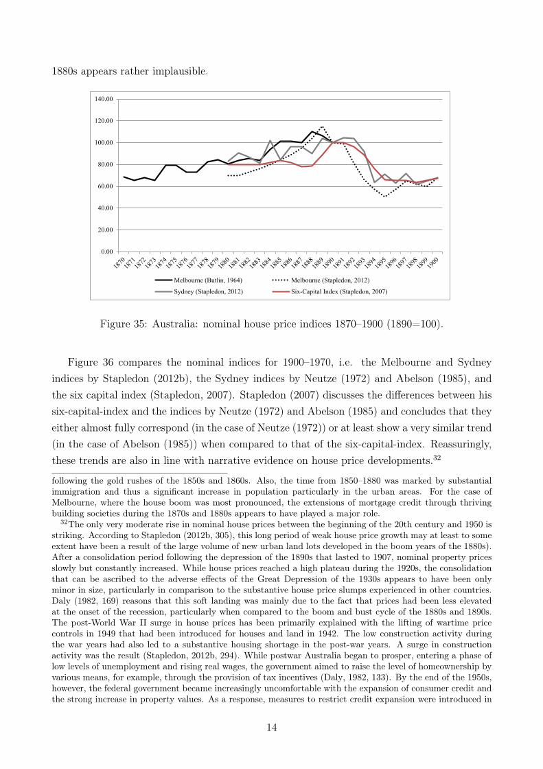
Figure 35 compares the nominal indices for 1860ndash1900 ie an index for Melbourne calcu-lated from Butlin (1964) the Melbourne and Sydney indices by Stapledon (2012b) and thesix capital index (Stapledon 2007) For the years they overlap (1880ndash1890) the four indicesprovide considerable indication of a boom-bust scenario albeit with peaks and troughs stag-gered between two to three years For the 1890s the indices generally show a positive trendwhich culminates between 1888 (Butlin 1964 Melbourne) and 1891 (Stapledon 2012b Syd-ney) The six-capitals-index follows a pattern that is somewhat disjoint and inconsistent withthat picture While from 1880 to 1887 prices are stagnant the boom period is limited to merethree years (1888ndash1891) during which the index reports a nominal increase of house prices inthe six capitals amounting to 25 percent This trajectory however not only differs from theMelbourne and Sydney indices but is also at odds with various accounts (Daly 1982 Stapledon2012b)31 Against this background the stagnation of the six-capital-index during most of the

28According to Stapledon (2007) this series gives a general impression of house price movements after 1860The series is based on advertisements of houses for sale in the newspapers Melbourne Age and Argus Stapledon(2007 16) reasons that by measuring the asking price in terms of rooms rather than houses Butlin partiallyadjusted for quality changes and differences as the average amount of rooms per dwelling rose considerablybetween 1861 and 1890

29The eight cities are Sydney Melbourne Brisbane Adelaide Perth Hobart Darwin Canberra rsquoProjecthomesrsquo are dwellings that are not yet completed In contrast the concept of rsquoestablished dwellingsrsquo refers toboth new and existing dwellings Locational structural and neighborhood characteristics are used to mix-adjust the index ie to control for compositional change in the sample of houses The series are constructedas Laspeyre-type indices The ABS commenced a review of its house price indices in 2004 and 2007 Priorto the 2004 review the index was designed as a price measure for mortgage interest charges to be included inthe CPI The weights used to calculate the index were thus housing finance commitments As part of the 2004review the pricing point has been changed the stratification method improved and the relative value of eachcapital cityrsquos housing stock used as weights In 2007 the stratification was again refined and the housing stockweights were updated Due to the substantive methodological changes of 2004 the ABS publishes two separatesets of indices 1986ndash2005 and 2002ndash2012 (Australian Bureau of Statistics 2009) They move however closelytogether in the years they overlap

30For 1960ndash2004 there also exists an unpublished index calculated by the Australian Treasury (Abelsonand Chung 2004) The index moves closely together with the one calculated by Abelson and Chung (2004)(correlation coefficient of 0995 for the period 1986ndash2003 and 0774 for 1970ndash1985) For the period 1970ndash2012an index is available from the OECD based on the house price index covering eight capital cities publishedby the Australian Bureau of Statistics For the period 1975ndash2012 the Federal Reserve Bank of Dallas splicestogether the index published by the Australian Bureau of Statistics (2013b) and the Treasury house price index

31Daly (1982) provides a graphical analysis of land and housing prices in Sydney for the period 1860ndash1940drawing on data from business records by Richardson and Wrench (at the time one of the largest real estateagents in Sydney) newspaper reports of sales and advertisements Daly (1982 150) and Stapledon (2012b)describe a pronounced property price boom during the 1880s followed by a bust in the 1890s The surge inreal estate prices was primarily spurred by a prolonged period of economic growth during the 1870s and 1880s

13

1880s appears rather implausible

000

2000

4000

6000

8000

10000

12000

14000

Melbourne (Butlin 1964) Melbourne (Stapledon 2012)

Sydney (Stapledon 2012) Six-Capital Index (Stapledon 2007)

Figure 35 Australia nominal house price indices 1870ndash1900 (1890=100)

Figure 36 compares the nominal indices for 1900ndash1970 ie the Melbourne and Sydneyindices by Stapledon (2012b) the Sydney indices by Neutze (1972) and Abelson (1985) andthe six capital index (Stapledon 2007) Stapledon (2007) discusses the differences between hissix-capital-index and the indices by Neutze (1972) and Abelson (1985) and concludes that theyeither almost fully correspond (in the case of Neutze (1972)) or at least show a very similar trend(in the case of Abelson (1985)) when compared to that of the six-capital-index Reassuringlythese trends are also in line with narrative evidence on house price developments32

following the gold rushes of the 1850s and 1860s Also the time from 1850ndash1880 was marked by substantialimmigration and thus a significant increase in population particularly in the urban areas For the case ofMelbourne where the house boom was most pronounced the extensions of mortgage credit through thrivingbuilding societies during the 1870s and 1880s appears to have played a major role

32The only very moderate rise in nominal house prices between the beginning of the 20th century and 1950 isstriking According to Stapledon (2012b 305) this long period of weak house price growth may at least to someextent have been a result of the large volume of new urban land lots developed in the boom years of the 1880s)After a consolidation period following the depression of the 1890s that lasted to 1907 nominal property pricesslowly but constantly increased While house prices reached a high plateau during the 1920s the consolidationthat can be ascribed to the adverse effects of the Great Depression of the 1930s appears to have been onlyminor in size particularly in comparison to the substantive house price slumps experienced in other countriesDaly (1982 169) reasons that this soft landing was mainly due to the fact that prices had been less elevatedat the onset of the recession particularly when compared to the boom and bust cycle of the 1880s and 1890sThe post-World War II surge in house prices has been primarily explained with the lifting of wartime pricecontrols in 1949 that had been introduced for houses and land in 1942 The low construction activity duringthe war years had also led to a substantive housing shortage in the post-war years A surge in constructionactivity was the result (Stapledon 2012b 294) While postwar Australia began to prosper entering a phase oflow levels of unemployment and rising real wages the government aimed to raise the level of homeownership byvarious means for example through the provision of tax incentives (Daly 1982 133) By the end of the 1950showever the federal government became increasingly uncomfortable with the expansion of consumer credit andthe strong increase in property values As a response measures to restrict credit expansion were introduced in

14

0

50

100

150

200

250

1900

1902

1904

1906

1908

1910

1912

1914

1916

1918

1920

1922

1924

1926

1928

1930

1932

1934

1936

1938

1940

1942

1944

1946

1948

1950

1952

1954

1956

1958

1960

1962

1964

1966

1968

1970

Sydney (Stapledon 2012) Melbourne (Stapledon 2012)

Sydney (Neutze 1972) Sydney (Abelson 1985)

Six Capital Cities (Stapledon 2007)

Figure 37 shows the indices which are available for the period 1970ndash2012 the Sydney andMelbourne indices by Stapledon (2012b) indices calculated from the Sydney and Melbourne se-ries by Abelson and Chung (2004) the six-capitals-index by Stapledon (2007) and the weightedindex for eight cities for 1986ndash2012 by the Australian Bureau of Statistics (2013b)33 Despitetheir different geographical coverage all indices for the years from 1970ndash2012 follow a jointalmost identical path It is only after 2004 that the increase in Melbourne property pricesshows to be more pronounced compared to Sydney or the Eight Capital Index

1960 The resulting credit squeeze had an immediate and sizable impact on both the real estate market andthe economy as whole (Stapledon 2007 56) The recovery from this brief interruption was rapid and propertyprices continued to boom

33The ABS series is spliced in 2003 As Stapledon (2012b) draws upon Abelson and Chung (2004) for 1970ndash1985 these series should therefore be identical for this period As Stapledon (2012b) uses the Australian Bureauof Statistics (2013b) series for Sydney and Melbourne for 1986ndash2012 these again should be identical for thisperiod In addition since Stapledon (2007) uses the Australian Bureau of Statistics (2013b) series for eightcapital cities these two indices are identical for post-1986 The Australian Bureau of Statistics (2013b) indexonly starts in 1986

15

0

50

100

150

200

250

300

350

400

450

1970

1971

1972

1973

1974

1975

1976

1977

1978

1979

1980

1981

1982

1983

1984

1985

1986

1987

1988

1989

1990

1991

1992

1993

1994

1995

1996

1997

1998

1999

2000

2001

2002

2003

2004

2005

2006

2007

2008

2009

2010

2011

2012

Eight Capital Cities (ABS 2013a) Sydney (Abelson and Chung 2004)

Melbourne (Abelson and Chung 2004) Six Capital Cities (Stapledon 2007)

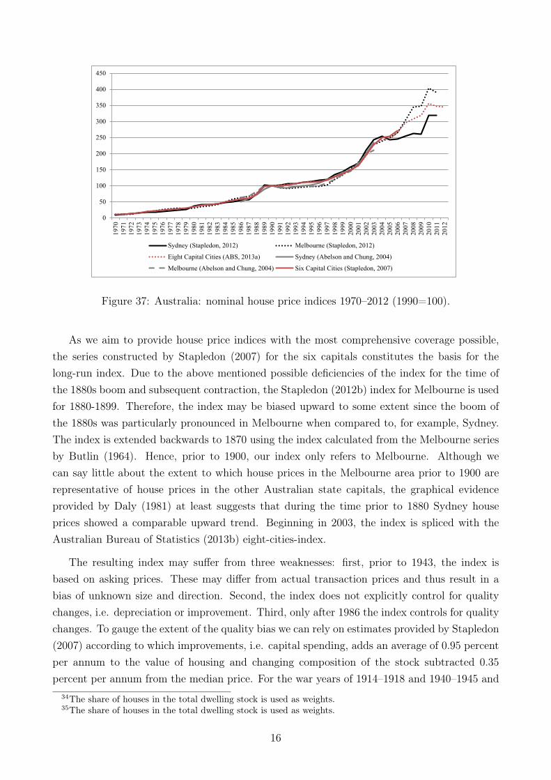
As we aim to provide house price indices with the most comprehensive coverage possiblethe series constructed by Stapledon (2007) for the six capitals constitutes the basis for thelong-run index Due to the above mentioned possible deficiencies of the index for the time ofthe 1880s boom and subsequent contraction the Stapledon (2012b) index for Melbourne is usedfor 1880-1899 Therefore the index may be biased upward to some extent since the boom ofthe 1880s was particularly pronounced in Melbourne when compared to for example SydneyThe index is extended backwards to 1870 using the index calculated from the Melbourne seriesby Butlin (1964) Hence prior to 1900 our index only refers to Melbourne Although wecan say little about the extent to which house prices in the Melbourne area prior to 1900 arerepresentative of house prices in the other Australian state capitals the graphical evidenceprovided by Daly (1981) at least suggests that during the time prior to 1880 Sydney houseprices showed a comparable upward trend Beginning in 2003 the index is spliced with theAustralian Bureau of Statistics (2013b) eight-cities-index

The resulting index may suffer from three weaknesses first prior to 1943 the index isbased on asking prices These may differ from actual transaction prices and thus result in abias of unknown size and direction Second the index does not explicitly control for qualitychanges ie depreciation or improvement Third only after 1986 the index controls for qualitychanges To gauge the extent of the quality bias we can rely on estimates provided by Stapledon(2007) according to which improvements ie capital spending adds an average of 095 percentper annum to the value of housing and changing composition of the stock subtracted 035percent per annum from the median price For the war years of 1914ndash1918 and 1940ndash1945 and

34The share of houses in the total dwelling stock is used as weights35The share of houses in the total dwelling stock is used as weights

16

Period Series

ID

Source Details

1870ndash1880 AUS1 Butlin (1964) Geographic Coverage Melbourne Type(s) ofDwellings All kinds of existing dwellings DataAdvertisements in newspapers Method Medianasking prices

1881ndash1899 AUS2 Stapledon (2012b) Geographic Coverage Melbourne Type(s) ofDwellings All kinds of existing dwellings DataAdvertisements in newspapers Method Medianasking prices

1900ndash1942 AUS3 Stapledon (2007) Geographic Coverage Six capital cities Type(s)of Dwellings All kinds of existing dwellingsData Advertisements in newspapers and Cen-sus estimates of average rents Method Medianasking prices

1943ndash1949 AUS4 Stapledon (2007) Geographic Coverage Six capital cities Type(s)of Dwellings All kinds of existing dwellingsData Estimate of the fixed price Method Es-timate of fixed price

1950-1972 AUS5 Stapledon (2007) Geographic Coverage Six capital cities Type(s)of Dwellings All kinds of existing dwellingsData Weekly property reports in newspapersand Census estimates of average rents Method Median sales prices

1973ndash1985 AUS6 Abelson and Chung(2004) as used inStapledon (2007)

Geographic Coverage Six capital cities Type(s)of Dwellings All kinds of existing dwellingsData Data from Land Title Offices (LTOs)Productivity Commission data Valuer-GeneralOffices Method Weighted average of medianprices34

1986ndash2002 AUS7 Australian Bureauof Statistics (2013b)as used in Stapledon(2007)

Geographic Coverage Six capital cities Type(s)of Dwellings New and existing detached housesData Data from State Valuer-General Officessupplemented by data on property loan appli-cations from major mortgage lenders Method Weighted average of mix-adjusted house priceindices35

2003ndash2012 AUS8 Australian Bureau ofStatistics (2013b)

Geographic Coverage Eight capital citiesType(s) of Dwellings New and existing de-tached houses Data Data from State Valuer-General Offices supplemented by data on prop-erty loan applications from major mortgagelenders Method Mix adjustment

Table 6 Australia sources of house price index 1870ndash2012

17

the depression periods 1891ndash1895 and 1930ndash1935 Stapledon (2007) assumes 055 percent perannum These estimates are in line with Abelson and Chung (2004) If we adjust the growthrates of our long-run series downward accordingly the average annual real growth rate over theperiod 1870ndash2012 of 168 percent becomes 111 percent in constant quality terms As this is arather crude adjustment we use the unadjusted index (see Table 6) for our analysis

Housing related data

Construction costs 1881ndash2012 Stapledon (2012a Table 2) - Construction costs of new dwellingsand alterations and additions

Residential land prices 1880sndash2005 Stapledon (2007 29 ff) - Real price series of lots atthe urban fringe period averages

Building activity 1956ndash2012 Australian Bureau of Statistics (2013a)

Homeownership rates 1911ndash2006 (benchmark dates) Australian Bureau of Statistics (var-ious years)

Value of housing stock Goldsmith (1985) and Garland and Goldsmith (1959) provide es-timates of the value of total housing stock dwellings and land for the following benchmarkyears 1903 1915 1929 1947 1956 1978 Data for 1988ndash2011 is drawn from OECD (2013)Piketty and Zucman (2014) present data on the value of household wealth in land and dwellingsfor 1959ndash2011

Household consumption expenditure on housing 1870ndash1939 Butlin (1985 Table 8) 1960ndash2012 Australian Bureau of Statistics (2014)

B3 Belgium

House price data

Historical data on house prices in Belgium is available for 1878ndash2012

The earliest available data on house prices in Belgium is provided by De Bruyne (1956) Itcovers the greater Brussels area for the period 1878ndash1952 and is reported as the annual medianprice per square meter of the interquartile range for four real estate categories i) residentialproperty36 in the center of Brussels ii) maisons de rentier37 iii) building sites (since 1885) and

36rsquoMaisons drsquohabitationrsquo are defined as houses of rather inferior quality Some of them may be rsquomaisons derentierrsquo (see below) that have been downgraded because of the neighborhood or the age of the building Theyare usually inhabited by workers or employees small and do not have electricity central heating gas or water(De Bruyne 1956 62)

37rsquoMaisons de rentierrsquo are defined as properties that are located in a good neighborhood have usually morethan one story are well maintained and serve as a single-family dwelling (De Bruyne 1956 61 f)

18

iv) commercial properties38 (since 1879)39

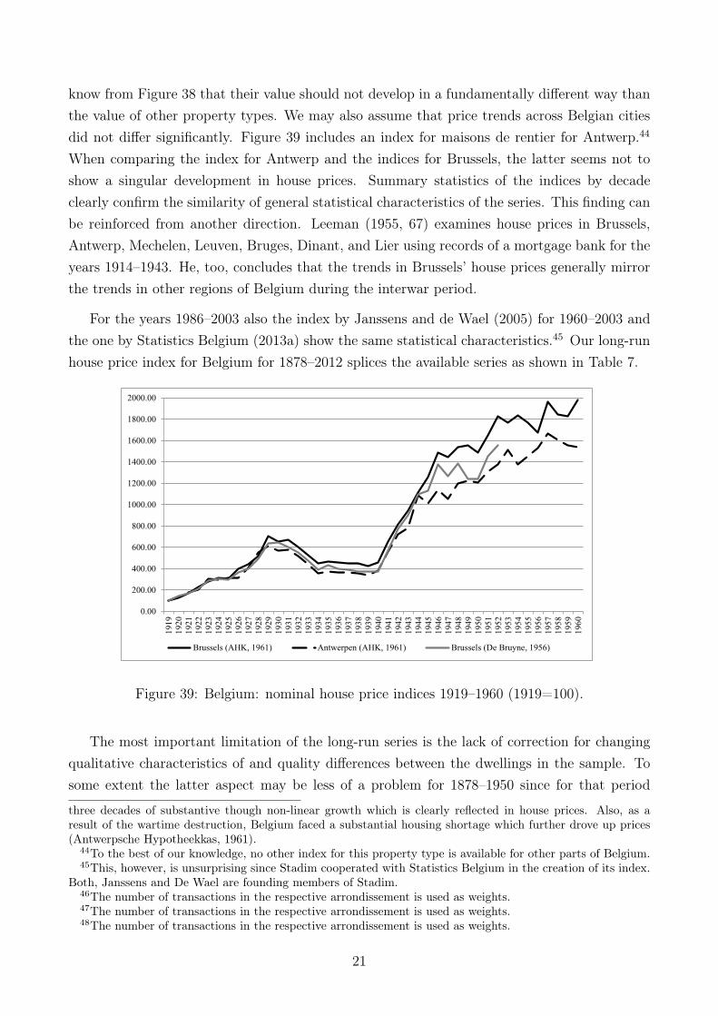
A second extensive source comprising two house price indices - one for 1919ndash1960 and theother for 1960ndash2003 - is Janssens and de Wael (2005) The first index ie for 1919ndash1960 isbased on two data sources for 1919ndash1950 the index relies on a property price index for Brusselspublished by the Antwerpsche Hypotheekkas (1961) using sales price data for maisons de rentierThe AHK-index is computed as the annual median price of the interquartile range For 1950ndash1960 the index is based on nationwide data for all public housing sales subject to registrationrights gathered by Statistics Belgium For these years the index reflects the development of theweighted mean sales price weights are constructed from the share of total national sales in eachof the 43 Belgian arrondissements (districts) The computational method for the second indexfrom Janssens and de Wael (2005) covering the years 1960ndash2003 is identical to that appliedto the sub-period 1950ndash1960 The sole difference lies in the coverage of the data provided byStatistics Belgium While for the period 1950ndash1960 sales information is limited to public salesthe index for the time 1960ndash2003 is computed using price information for both public andprivate housing sales that were subject to registration rights

In addition to these two principal sources for the years since 1986 Statistics Belgium(2013a) on a quarterly basis publishes price indices for the following four types of real estatei) building lots ii) apartments iii) villas and iv) single-family dwellings The indices areconstructed using stratification and are available for the national regional district (arrondisse-ments) and communal level40

Figure 38 shows the nominal indices for the different property types (maisons drsquohabitationmaisons des rentier commercial buildings and building sites) based on the data from De Bruyne(1956) Three indices (maison drsquo habitation maison de rentier and maison de commerce)move closely together throughout the 1878ndash1913 period only the building sites index shows acomparably higher degree of volatility particularly during the 1880s and 1890s Neverthelessall four indices depict a similar trend nominal house prices trend downwards until the late

38Commercial properties are defined as all buildings for commercial use ie hotels restaurants retail storeswarehouses etc (De Bruyne 1956 63)

39The data is drawn from accounts of public real estate sales published in the Guide de lrsquoExpert en Immeubles(Real Estate Agentsrsquo Catalogue) a periodical of the Union des Geacuteomegravetres-Experts de Bruxelles (Union ofSurveyors of Brussels) The records include the more urban parts of the Brussels district such as Brusselsitself Etterbeek Ixelles Molenbeek Saint-Gilles Saint-Josse Schaerbeek Koekelberg and Laeken De Bruyne(1956) also publishes separate house price series for the more rural areas such as Anderlecht AuderghemForest Ganshoren Jette Uccle Watermael-Boitsfort Berchem-Ste-Agathe Woluwe-St-Lambert Woluwe-St-Pierre Evere Haeren Neder over-Heembeck

40Dwellings are stratified according to type and location The stratification was refined in 2005 so that single-family dwellings are categorized according to their size (small average large) causing a break in the seriesbetween 2004 and 2005 The index is computed as a chain Laspeyre-type price index It does not controlfor quality changes Districts are aggregated according to the number of dwellings in the base period (2005)For the period 1970ndash2012 an index is available from the OECD based on the index compiled by the Bank ofBelgium which in turn is based on the data from Statistics Belgium (European Central Bank 2013) For theperiod 1975ndash2012 the Federal Reserve Bank of Dallas also uses the data from Statistics Belgium (2013a) andStadim (2013)

19

1880s and slowly recover afterwards De Bruyne (1956) suggests that these trends are generallyin line with the fundamental macroeconomic trends and narrative evidence on house pricedevelopments in Belgium41

2000

4000

6000

8000

10000

12000

14000

1600018

7818

7918

8018

8118

8218

8318

8418

8518

8618

8718

8818

8918

9018

9118

9218

9318

9418

9518

9618

9718

9818

9919

0019

0119

0219

0319

0419

0519

0619

0719

0819

0919

1019

1119

1219

13

Maisons dHabitation (De Bruyne 1956) Maisons des Rentier - Urban (De Bruyne 1956)

Maisons de Commerce (De Bruyne 1956) Sites - Urban (De Bruyne 1956)

Figure 38 Belgium nominal house price indices 1878ndash1913 (1913=100)

Figure 39 displays the nominal indices available for 1919ndash1960 ie the index calculated fromthe data by De Bruyne (1956) for the Brussels area the indices from Janssens and de Wael(2005) for the Brussels area and an index for Antwerp by Antwerpsche Hypotheekkas (1961)As Figure 39 shows these nominal indices move closely together during the years they overlapie 1919ndash195242 The indices accord with accounts of house price developments during thisperiod43 Although all three indices only gauge price developments for maisons de rentier we

41Since the 1880s the Belgian economy had been in a recession Recovery only began to take hold in themid-1890s (Van der Wee 1997) The housing act of 1899 through promoting reduced-rate loans and extendingtax exemptions and tax reduction for homeowners may have further contributed to the slow upward trend inhouse prices (Van den Eeckhout 1992) Following the economic resurgence in 1906 Belgium until the eve ofWorld War I experienced years of prospering economic activity De Bruyne (1956) notes that during this periodthe gap between prices for property in urban and more peripheral parts of the Brussels area began to close Heascribes this convergence largely to improvements in transportation and communication systems during thattime (Janssens and de Wael 2005 Antwerpsche Hypotheekkas 1961)

42Correlation coefficient of 0995 for the two Brussels indices correlation coefficient of 0993 for the Antwerpen-index (Antwerpsche Hypotheekkas 1961) and the Brussels index (De Bruyne 1956)

43De Bruyne (1956) reasons that the increase in property prices between 1919 and 1922 was to a large extentcaused by a general shortage of housing in the postwar years While De Bruyne (1956) in this context diagnosesthe house price boom to be primarily driven by speculation the Antwerpsche Hypotheekkas (1961) attributesthe price rise to the rapid economic growth during these years House prices substantially decreased throughoutthe economic crisis of the 1930s De Bruyne (1956) however argues that the decrease was less pronouncedin less expensive property categories ie maisons drsquohabitation as opposed to maisons de rentier since withdeclining incomes many people were forced to relocate to either areas in which housing is less expensive or tolower quality housing Prices appear to slightly recover in the end of the 1930s Yet the advent of World WarII puts the property market back into decline After the end of World War II the Belgian economy entered

20

know from Figure 38 that their value should not develop in a fundamentally different way thanthe value of other property types We may also assume that price trends across Belgian citiesdid not differ significantly Figure 39 includes an index for maisons de rentier for Antwerp44

When comparing the index for Antwerp and the indices for Brussels the latter seems not toshow a singular development in house prices Summary statistics of the indices by decadeclearly confirm the similarity of general statistical characteristics of the series This finding canbe reinforced from another direction Leeman (1955 67) examines house prices in BrusselsAntwerp Mechelen Leuven Bruges Dinant and Lier using records of a mortgage bank for theyears 1914ndash1943 He too concludes that the trends in Brusselsrsquo house prices generally mirrorthe trends in other regions of Belgium during the interwar period

For the years 1986ndash2003 also the index by Janssens and de Wael (2005) for 1960ndash2003 andthe one by Statistics Belgium (2013a) show the same statistical characteristics45 Our long-runhouse price index for Belgium for 1878ndash2012 splices the available series as shown in Table 7

000

20000

40000

60000

80000

100000

120000

140000

160000

180000

200000

1919

1920

1921

1922

1923

1924

1925

1926

1927

1928

1929

1930

1931

1932

1933

1934

1935

1936

1937

1938

1939

1940

1941

1942

1943

1944

1945

1946

1947

1948

1949

1950

1951

1952

1953

1954

1955

1956

1957

1958

1959

1960

Brussels (AHK 1961) Antwerpen (AHK 1961) Brussels (De Bruyne 1956)

The most important limitation of the long-run series is the lack of correction for changingqualitative characteristics of and quality differences between the dwellings in the sample Tosome extent the latter aspect may be less of a problem for 1878ndash1950 since for that period

three decades of substantive though non-linear growth which is clearly reflected in house prices Also as aresult of the wartime destruction Belgium faced a substantial housing shortage which further drove up prices(Antwerpsche Hypotheekkas 1961)

44To the best of our knowledge no other index for this property type is available for other parts of Belgium45This however is unsurprising since Stadim cooperated with Statistics Belgium in the creation of its index

Both Janssens and De Wael are founding members of Stadim46The number of transactions in the respective arrondissement is used as weights47The number of transactions in the respective arrondissement is used as weights48The number of transactions in the respective arrondissement is used as weights

21

Period Series

ID

Source Details

1878ndash1913 BEL1 De Bruyne (1956) Geographic Coverage Brussels area Type(s) ofDwellings Existing maisons de rentier DataGuide de lrsquoExport en Immeubles Method Me-dian sales prices

1919ndash1950 BEL2 Janssens and de Wael(2005) based onAntwerpsche Hy-potheekkas (1961)

Geographic Coverage Brussels area Type(s) ofDwellings Maisons de Rentier Data Antwerp-sche Hypotheekkas (1961) Method Mediansales prices

1951ndash1959 BEL3 Janssens and de Wael(2005)

Geographic Coverage Nationwide Type(s)of Dwellings Small amp medium-sized exist-ing houses Data Transaction prices (publicsales gathered by Statistics Belgium) Method Weighted average of mean sales prices46

Geographic Coverage Nationwide Type(s) ofDwellings 1960ndash1970 Small amp medium-sizedexisting houses 1971 onwards all kinds of ex-isting dwellings (villas amp mansions included)Data Transaction prices (public and privatesales) gathered by Statistics Belgium) Method Weighted average of mean sales prices47

1986-2012 BEL5 Statistics Belgium(2013a)

Geographic Coverage Nationwide Type(s) ofDwellings Existing single-family dwellingsData Transaction prices Method Weightedmix-adjusted index48

Table 7 Belgium sources of house price index 1878ndash2012

22

the index is confined to a certain market segment ie maisons de rentier Prior to 1950 theseries is also adjusted for the size of the dwelling as it is based on price data per square meterMoreover despite the fact that the movements in prices for maisons de rentier closely mirrorfluctuations in prices of other property types prior to 1913 (cf Figure 38) it is of course possiblethat this particular market segment is not perfectly representative of fluctuations in prices ofother residential property types for the whole 1878ndash1950 period In an effort to gauge the sizeof the upward bias stemming from quality improvements we calculate the value of expenditureson alterations and additions as percentage in total housing value for benchmark years If wedownward adjust the real annual growth rates of our long-run index accordingly the averageannual real growth rate over the period 1878ndash2012 of 196 percent becomes 177 percent inconstant quality terms Yet as this is a rather crude adjustment we use the unadjusted index(see Table 7) for our analysis

Construction costs 1914ndash2012 Belgian Association of Surveyors (2013) - Construction costindex for new buildings and dwellings 1890ndash1961 (additional) Buyst (1992) - Index for buildingmaterial prices (excluding wages)

Farmland prices 1953ndash2007 Vlaamse Overheid49 - Price index for farmland 2008ndash2009Bergen (2011) - Sales prices for farmland in Vlaanderen per square meter50

Residential land prices 1953ndash2012 Stadim (2013) - Prices of building lots

Building activity 1890ndash1961 Buyst (1992) 1927-1950 Leeman (1955)

Homeownership rate 1947ndash2009 (benchmark dates) Van den Eeckhout (1992)

Value of housing stock Goldsmith (1985) provides estimates of the value of total housingstock dwellings and land for 1950 and 1978 Data for 2005ndash2011 is drawn from Poullet (2013)

Household consumption expenditure on housing 1953ndash1959 Statistics Belgium (1994)1960ndash1994 Statistics Belgium (1998) 1995ndash2012 Statistics Belgium (2013b)

B4 Canada

House price data

Historical data on house prices in Canada is scarce even though real estate boards were alreadyestablished in the early 20th century Data on house prices in Canada is available for 1921ndash2012

49Series sent by email contact person is Els Demuynck Vlaamse Overheid50No data is available for 2010ndash2012

23

The first available series is presented by Firestone (1951) and covers the years 1921ndash1949The index is calculated using data on the average value of residential real estate (includingland) and the number of existing dwellings and hence reflects the average replacement value ofexisting dwellings rather than prices realized in transactions51

A dataset published by the Canadian Real Estate Association (1981 (CREA)) covers thetime 1956ndash1981 It contains annual data on the average value and the number of transactionsrecorded in the Canadian Multiple Listing System (MLS) for all properties ie it includesboth residential and non-residential real estate In addition Subocz (1977) presents a meanprice index for new and existing single-family detached houses covering an earlier period ie1949ndash1976 The index is based on price data collected from the records of the Vancouver andNew Westminster Registry offices serving the Greater Vancouver Regional District

CREA also publishes a second house price data series that solely draws on price data fromsecondary market residential properties transactions through MLS covering the years 1980ndash201252 The series is computed as average of all sales prices in the residential property market

The University of British Columbia index constitutes another source for the development ofhouse prices in Canada It covers the period 1975ndash2012 and is computed from price informationfor existing bungalows and two story executive detached houses in ten main metropolitan areasof Canada (Centre for Urban Economics and Real Estate University of British Columbia2013 UBC Sauder)53 For each of the cities UBC Sauder uses a population weighted averageof the price change in each neighborhood for which data is available Subsequently the index isweighted on changes in the price level of different housing types ie detached bungalows andexecutive detached houses according to their share in total units sold The aim is to capturethe within-metro-variation in house prices in proportion to the size of the housing stock andvariation across housing types The data is drawn from the Royal LePage house price survey54

51Firestone (1951 431 ff) calculates the value of residential capital ie the value of all existent dwellingsin 1921 by computing the average construction cost per dwelling adjusting it for the proportion of the life ofthe dwelling already consumed and multiplying it with the number of available dwellings The adjustment wasmade by subtracting 2275 of the average cost of a non-farm home (the average age of a non-farm home in 1921was 22 years Firestone (1951) assumes an average life expectancy of a dwelling of 75 years) and 1860 for farmhomes (the average age of a farm home in 1921 was 18 years Firestone (1951) assumes an average life expectancyof a farm dwelling of 60 years) The resulting value for 1921 may thus underestimate the value of an averageresidential structure in 1921 as it is not adjusted for improvements or alterations of the existing housing stockUsing these estimates of the value of structures and data on the ratio of land cost to construction costs Firestone(1951) calculates the value of residential land in 1921 For the years 1922ndash1949 the 1921 value is revalued usingaverage construction costs deducting depreciation deducting the value of destroyed and damaged dwellingsand adding gross residential capital formation in the respective year The value of land put in use for residentialuse in the respective year is added and the value of land removed from residential use is deducted The seriesfor the total value of residential real estate is calculated as the sum of the series for the value of structures andthe series for the value of land

52Series sent by email contact person is Gregory Klump Canadian Real Estate Association (CREA)53Bungalows are defined as detached one-story three-bedroom dwellings with living space of about 111 square

meters54The way the house price survey is conducted ensures some degree of constant quality as Royal LePage

standardizes each housing type according to several criteria such as square footage the number of rooms etc

24

In addition to that Statistics Canada issues three house price indices for new developmentsData are disaggregated to the provincial level and currently cover the period 1981ndash2012 Theymeasure price developments for i) buildings ii) land and iii) real estate (land and buildings)and are aggregated to nationwide indices and a separate index for the Atlantic region (StatisticsCanada 2013c) The indices are computed from sales prices of new real estate constructed bycontractors based on a survey that is conducted in 21 metropolitan areas with the number ofbuilders in the sample representing at least 15 percent of the total building permit value ofthe respective city and year The construction firms covered mainly develop single unit housesThe survey data includes information on various characteristics of the units constructed andsold The index is a matched-model index ie a constant-quality index in the sense that thecharacteristics of the structures and the lots are identical between successive periods

The index produced by Firestone (1951) is hence the only available source for house pricesin Canada prior to the 1950s We therefore have to rely on accounts of housing market devel-opments as plausibility check The nominal index suggests that house prices are fairly stablethroughout the 1920s fall in the wake of the Great Depression and increase after 1935 An-derson (1992) discussing Canadian housing policies in the interwar period also suggests thathouse prices fall during the early 1930s He furthermore points toward policy measures in-troduced during the second half of the 1930s that aimed at stimulating housing constructionwhich may explain a demand-driven increase in house prices during these years55 Overall thetrajectory of the Firestone (1951) appears plausible

Figure 40 compares the nominal house price indices available for 1956ndash2012 ie the UBCSauder index the price index for new houses (including land) by Statistics Canada and anindex computed from the two CREA datasets (ie 1956ndash1981 and 1980ndash2012) As the graphsuggests all indices show a marked positive trend in the post-1980 period However themagnitude of the price increase varies between the four measures The European Commission(2013 120) suggests that the more pronounced growth of the CREA index since the mid-1980sis due to the fact that the series is calculated from a simple average of real estate secondarymarket prices Hence it is biased with respect to the composition (eg size standard qualityetc) of the overall volume of secondary market transactions As this second CREA indexdue to the substantive coverage of MLS includes about 70 percent of all marketed residentialproperties (European Commission 2013 119) it can despite these conceptual limitations beconsidered a fairly reliable measure for the overall evolution of house prices in Canada for thetime from 1980 to present In comparison to the CREA index the Statistics Canada index fornew houses points toward a less pronounced increase in house prices However this StatisticsCanada index - as it is solely calculated from price information on new developments - mayalso be subject to some degree of bias New residential developments are primarily built in the

(European Commission 2013 119)55Anderson (1992) lists the 1935 Dominion Housing Act the 1937 Home Improvement Loan Guarantee Act

and the 1938 National Housing Act

25

suburban areas of larger agglomerations where prices and price fluctuations tend to be lowerthan in city centers (Statistics Canada 2013a European Commission 2013) This may alsobe the reason for the different magnitude between the UBC Sauder index and the index byStatistics Canada For the years since 1975 we use the UBC Sauder index as it is confinedto a certain market segment (bungalows and existing two-story executive buildings) and thusshould be less prone to composition bias than the CREA series56

000

10000

20000

30000

40000

50000

60000

MLS All Property Types (CREA 1981)

MLS Residential Property (CREA 2012)

New Housing Price Index Land and House (Statistics Canada 2013c)

UBC Sauder

Figure 40 Canada nominal house price indices 1956ndash2012 (1981=100)

Figure 41 compares the CREA index for 1956ndash1981 with the one presented by Subocz (1977)CREA argues that the MLS statistics covering residential and non-residential real estate forthe time from 1956ndash1981 can be used to reliably proxy residential house price development Inaddition to the CREA index and the Subocz index two other sources discuss the developmentof Canadian house prices prior to the 1980s The first is a report by Miron and Clayton (1987)which is commissioned by the Canada Mortgage and Housing Corporation and the housingagency of the Canadian government The authors use scattered data from Statistics Canadato discuss developments in house prices in Canada between 1945 and 198657 Their narrativesuggests that house prices in the postwar period generally followed the development of theCanadian economy as a whole According to the authors postwar social policy schemes -even though not directly linked to housing policy - generated additional demand side effects asthey enabled particularly low-income families to devote a larger disposable income to housingconsumption House prices strongly increased during postwar years ie until the late 1950s

56Figure 40 suggests that the CREA index for the time 1975ndash1980 follows a trend different from that of theUBC and Statistics Canada indices While the latter for the period under consideration show a considerablepositive trend the former appears to be fairly stagnant We therefore also use the UBC Sauder index for theyears 1975ndash1980

57Years included 1941 1946 1951 1956 1961 1966 1971 1976 1981 1984

26

when economic growth declined creating a decline in house prices In the economic resurgencestarting in the mid-1960s house prices also picked-up and increased at a frantic pace in the1970s before tailing off again in the recession of the 1980s (Miron and Clayton 1987 10)58

A second source is Poterba (1991) who also identifies a run-up in house prices during the 1970sthat coincided with the recession of 1982 With the pattern of pronounced variation in thegrowth rates of real estate prices over time as diagnosed by Miron and Clayton (1987) andPoterba (1991) the first CREA index must be treated with caution It shows that differentto the CREA-index the Sobocz-index appears more consistent with narratives by Miron andClayton (1987) and Poterba (1991) for the period 1949ndash1976 Yet the Sobocz-index relies onlyon a rather small sample size and is confined to property sales in the Greater Vancouver areaAnother sign of partial inconsistency is the fact that the Sobocz-index reports an increase inaverage real house prices of an astonishing 280 percent between 1956 and 1974 The CREAindex for the same time reports an increase of approximately 87 percent Therefore despite itspotential weaknesses we rely on the CREA index to construct the long-run house price indexfor Canada

000

5000

10000

15000

20000

25000

1949

1951

1952

1953

1954

1955

1956

1957

1958

1959

1960

1961

1962

1963

1964

1965

1966

1967

1968

1969

1970

1971

1972

1973

1974

1975

1976

1977

1978

1979

1980

1981

Subocz (1977) MLS All Property Types (CREA 1981)

Data on residential house prices is available for 1921ndash1949 and for 1956 onwards For 1921ndash1949 the series on average value of existing farm and existing non-farm dwellings includingland are highly correlated (Firestone 1951 Tables 69 amp 80)59 Since no data on residentialhouse prices is available for 1949ndash1956 we use the percentage change in the value of farm real

58Miron and Clayton (1987) argue that the house price surge during the 1970s was also associated with thebaby boomers starting to buy residential properties They also suggest that tax policies made homeownershipmore attractive after the tax reforms of 1972 introducing tax exemption of capital gains from sales of principalresidences

59Correlation coefficient of 0856

27

Period Series

ID

Source Details

1921-1949 CAN1 Firestone (1951) Geographic Coverage Nationwide Type(s) ofDwellings All kinds of existing dwellings (farmand non-farm) Data Estimates of the value ofresidential structures and the value of residentialland as well as data on all available residentialdwellings Method Average replacement values

1949-1956 Urquhart and Buckley(1965)

Geographic Coverage Nationwide Type(s) ofDwellings Farm real estate Method Value offarm real estate per acre

1956-1974 CAN2 Canadian Real EstateAssociation (1981)

Geographic Coverage Nationwide Type(s) ofDwellings All kinds of real estate (residentialand non-residential) Data Transactions regis-tered in the MLS system Method Average salesprices

1975-2012 CAN3 Centre for Urban Eco-nomics and Real EstateUniversity of BritishColumbia (2013)

Geographic Coverage Five cities Type(s) ofDwellings Existing bungalows and two story ex-ecutive dwellings Data Royal LePage real es-tate experts Method Average prices

Table 8 Canada sources of house price index 1921ndash2012

estate per acre to link the 1921ndash1949 and the 1956ndash1974 series (Urquhart and Buckley 1965)Our long-run house price index for Canada 1921ndash2012 splices the available series as shown inTable 8

The resulting long-run index has three drawbacks first data prior to 1949 is not basedon actual list or transaction prices but calculated as the average replacement value of existingdwellings including land value (see data description above) This approach may result in a biasof unknown size and direction Second for 1956ndash1974 the index refers to both residential andnon-residential real estate and is not adjusted for compositional changes Third the index isnot adjusted for quality improvements for the years after 1956 The bias should be mitigatedfor the post-1975 years due to the way the Royal LePage survey is set up (see above) As away to gauge the potential effect of quality changes we calculate the value of expenditures onalterations and additions as percentage in total housing value for benchmark years and adjustthe annual growth rates of the series downward for the years 1956ndash1974 using these estimatesThe average annual real growth rate over the period 1921ndash2012 of 221 percent becomes 167percent in constant quality terms As this is a rather crude adjustment we use the unadjustedindex (see Table 8) for our analysis

Construction costs 1952ndash1976 Statistics Canada (1983 Tables S326-335) - Residential build-ing construction input price index 1977ndash1985 Statistics Canada (various yearsb) - Residential

28

building construction input price index 1986ndash2012 Statistics Canada (2013b) - Price index ofapartment construction (seven census metropolitan composite index)

Farmland prices 1901ndash1956 Urquhart and Buckley (1965) - Value of farm capital (landand buildings) per acre 1965ndash2009 Manitoba Agriculture Food and Rural Initiatives (2010)- Value of farm real estate (land and buildings) per acre 2010ndash2011 Province of Manitoba(2012) - Value of farm real estate (land and buildings) per acre

Building activity 1921ndash1949 Firestone (1951 Table 22) 1957ndash2012 Statistics Canada(2014)

Homeownership rates (benchmark dates) Miron (1988) Statistics Canada (1967) StatisticsCanada (2011)

Value of housing stock Goldsmith (1985) provides estimates of the value of total housingstock dwellings and land for the following benchmark years 1950 and 1978 Data on thevalue of household wealth including the value of total housing stock dwellings and land for1970-2011 is drawn from OECD (2013) Piketty and Zucman (2014) also present data on realestate wealth for benchmark years in the period 1895ndash1955

Household consumption expenditure on housing 1926ndash1946 Statistics Canada (2001)1961ndash1980 Statistics Canada (2012) 1981ndash2012 Statistics Canada (2013d)

B5 Denmark

House price data

Historical data on house prices in Denmark is available for 1875ndash2012

The most comprehensive source for house prices in Denmark is Abildgren (2006) Abildgren(2006) provides a price index for single-family houses in Denmark for the period 1938ndash2005and a price index for farms covering the time 1875ndash2005 The index for single-family housesreflects annual average sales prices and is computed using data from Oslashkonomiministeret (19661938ndash1965)60 Danmarks Nationalbank (various years) and Statistics Denmark (various yearsa1966ndash2005) The index for farms reflects the sales price per unit of land valuation based onestimated productivity61 for 1875ndash1959 and average sales prices per farm for 1960ndash200562

60Oslashkonomiministeret (1966) publishes an index on the average sales price of single-family houses for fivedifferent geographical areas i) Copenhagen and Frederiksberg ii) provincial towns iii) Copenhagen areaiv) towns with more than 1500 inhabitants and v) other rural communities Until 1950 the indices refer toproperties with a value of 20000 Danish crowns or less From 1951 onwards they are based on the averagepurchase price of properties containing one apartment According to Oslashkonomiministeret (1966) the break inthe series may cause an upward bias for 1950ndash1951

61Land was valued according to barrel of hartkorn ie barley and rye produced Thus the data refers tothe price paid per barrel of hartkorn

62The index is computed using sales price data for all farms for 1960ndash1967 for farms between 10 and 100

29

A second important source for property price development in Denmark is provided by theDanish Central Bank63 Drawing on data from the Ministry of Taxation (SKAT) and usingthe Sale-Price-Appraisal-Ratio (SPAR) as computational method the bank publishes a quar-terly house price series covering data for new and existing single-family dwellings since 1971(Danmarks Nationalbanken 2003)

A third source is Statistics Denmark (2013a) The agency publishes a nationwide houseprice index for single-family houses as well as for several types of multifamily structures forthe time 1992ndash2012 As in the case of the index by the Danish Central Bank the index byStatistics Denmark is computed using the SPAR method (Mack and Martiacutenez-Garciacutea 2012)

As shown in Figure 42 the property price indices for farms and for single-family houses arestrongly correlated for the years they overlap ie for the years since 193864 Kristensen (200712) estimates that at the end of World War II about 50 percent of the Danish population livedin rural areas Thus farm property accounted for a significant share of total Danish propertyand may be used as a proxy for Danish house prices prior to 1938 Nevertheless the series for1875ndash1937 must be treated with caution when analyzing house price fluctuations in Denmark inthis period65 Reassuringly the farm price index for the time prior to World War I appears tocoherently mirror the general development of the Danish economy during that period (Nielsen1933) and generally accords with accounts of developments in the housing market (Hyldtoft1992) Finally as shown in Figure 43 when comparing the single-family house price indices for1938ndash1965 the development of house prices in urban areas does not seem to systematically differfrom house prices in rural areas It is only in the 1960s that urban areas show substantivelystronger house price growth compared to rural areas

hectare for 1968ndash1975 and for farms between 15 and 60 hectare for 1976ndash2005 Data is drawn from StatisticsDenmark (various yearsa) Statistics Denmark (various yearsb) Hansen and Svendsen (1968) and StatisticsDenmark (1958)

63Series sent by email contact person is Tina Saaby Hvolboslashl Danish Central Bank64Correlation coefficient of 0996 for 1938ndash2005 See also Abildgren (2006 31)65In 1895 the Danish economy entered a ten year long boom period During the boom years many newly

established banks extended credit to finance a building boom in Copenhagen that developed into a price bubblein the market for residential property The optimism started to wane in 1905 and prices substantially contractedduring the financial crisis of 1907 (Oslashstrup 2008 Nielsen 1933 Hyldtoft 1992) The price index for farms doeshowever not reflect such a boom-bust pattern There are two possible explanations that may have joint orpartial validity First since the construction boom was centered in the residential real estate sector the indexfor farm prices may not provide an adequate picture of developments in house prices Second as the constructionboom was concentrated in Copenhagen the boom and bust may not be visible on the national level

30

000

5000

10000

15000

20000

25000

30000

1938

1940

1942

1944

1946

1948

1950

1952

1954

1956

1958

1960

1962

1964

1966

1968

1970

1972

1974

1976

1978

1980

1982

1984

1986

1988

1990

1992

1994

1996

1998

2000

2002

2004

House Price Index Farm Price Index

Figure 42 Denmark nominal house and farm price indices 1938ndash2005 (1995=100)

The index for single-family houses by Abildgren (2006) and the index by Statistics Denmark(2013a) show to be highly correlated for the years they overlap (1992ndash2010)66 This is also thecase for the index by Danmarks Nationalbanken the index by Statistics Denmark (2013a) andthe one by Abildgren (2006)67 To keep the number of data sources to construct an aggregateindex to the minimum the here composed long-run index relies on Danmarks Nationalbankenindex for the period since 1971 Our long-run house price index for Denmark 1875ndash2012 splicesthe available series as shown in Table 9

66Correlation coefficient of 0971 for 1992ndash201067The series constructed by Statistics Denmark (2013a) and Danmarks Nationalbanken have a correlation

coefficient of 0999 for 1992ndash2012 The series constructed by Abildgren (2006) and Danmarks Nationalbankenhave a correlation coefficient of 0999 for 1971ndash2005

31

Period Series

ID

Source Details

1875ndash1938 DNK1 Abildgren (2006) Geographic Coverage Nationwide Type(s) ofDwellings Existing farms Data Data from var-ious sources (see text) Method Average prices

1939ndash1971 DNK2 Abildgren (2006) Geographic Coverage Nationwide Type(s) ofDwellings Existing single-family houses DataData drawn from various sources (see text)Method Average prices

1972ndash2012 DNK3 Danmarks National-banken

Geographic Coverage Nationwide Type(s)of Dwellings New and existing single-familyhouses Data Ministry of Taxation (SKAT)Method SPAR method

Table 9 Denmark sources of house price index 1875ndash2012

000

10000

20000

30000

40000

50000

60000

70000

80000

90000

Copenhagen amp Frederiksberg Provincial towns

Copenhagen area Towns with more than 1500 inhabitants

Rural communities

Figure 43 Denmark nominal single-family house price indices 1938ndash1965 (1938=100)

The resulting long-run index has two weaknesses first the series used for 1875ndash1938 onlyreflects the price development of farm property which may deviate to some extent from pricedevelopments of other residential properties Second the series used for 1875ndash1970 is adjustedneither for compositional changes nor for quality changes To gauge the extent of the qualitybias we can rely on estimates of the quality effect by Lunde et al (2013) If we adjust thereal annual growth rates of our long-run index downward accordingly the average annual realgrowth rate over the period 1875ndash2012 of 099 percent becomes 057 percent in constant qualityterms Yet as this is a rather crude adjustment we use the unadjusted index (see Table 9) forour analysis

32

Construction costs 1913ndash2012 Statistics Denmark (various yearsb) - Building cost index

Farmland prices 1875ndash2005 Abildgren (2006) - Index for farm property prices 1870ndash1912OrsquoRourke et al (1996) - Index for agricultural land values

Land prices 1938ndash1965 Oslashkonomiministeret (1966) - Building sites below 2000 squaremeters

Building activity 1917ndash1980 Johansen (1985 Table 37b) - Number of new flats 1950ndash2011 Statistics Denmark (various yearsb) - Residential dwellings started

Homeownership rates 1930ndash2013 (benchmark years) Statistics Denmark (2013b)

Value of housing stock Goldsmith (1985) provides estimates of the value of total housingstock dwellings and land for the following benchmark years 1880 1900 1913 1929 19381948 1960 1965 1973 1978

Household consumption expenditure on housing 1870ndash2012 Statistics Denmark (2014)

B6 Finland

House price data

Historical data on house prices in Finland is available for 1905ndash2012

The earliest series at our disposal covers the period 1904ndash1962 It reports average annualprices of building sites for dwellings per square meter offered for sale by the city of Helsinki(Statistical Office of the City of Helsinki various years) Drawing on this data source weconstruct a three-year-average price index for residential building sites for 1905ndash1961 to smoothout some of the year-to-year fluctuations stemming from variation in the number of transactions

A second important source for property price development is Levaumlinen (1991) Levaumlinen(1991 39) using data from different sources computes a building site price index comprisingthe period 1909ndash198968 The index is primarily calculated from price data for sites for detachedand terraced houses in Southern Finland particularly in the Helsinki area Recently Levaumlinen(2013) has been able to update his original index such that it now covers the years 1910ndash2011Data for the more recent period 1989ndash2011 is taken from the National Land Survey of Finlandstatistics

A third source that covers the more recent development of residential property prices (1985ndash68The index is a chain index constructed from several indices for shorter sub-periods He then calculates the

ratios of every two successive years The resulting index is calculated based on all the ratios between the yearsFor years for which several data sources are available Levaumlinen uses a simple average

33

2012) is Statistics Finland The agency constructs a nationwide house price index for existingsingle-family dwellings and single-family house plots using a combination of hedonic regressionand a mix-adjusted method69 Statistics Finland uses data from the real estate register of theNational Land Survey containing all real estate transactions (Saarnio 2006 Statistics Finland2013c) A second Statistics Finland index based on the same computational procedure (hedonicregression and mix-adjusted method) and covering the same time period (1985ndash2012) reportsprice development for existing dwellings in so-called housing companies that is block of flatsand terraced houses The index is estimated from asset transfer tax statements of the TaxAdministration (Saarnio 2006 Statistics Finland 2011)70

As one component of its index for dwellings in housing companies Statistics Finland pro-vides estimates for average prices per square meter of dwellings in old blocks of flats71 in thecenter of Helsinki for the period 1947ndash2012 and for greater Helsinki72 and Finland as a whole forthe period 1970ndash201273 For the years prior to 1987 Statistics Finland relies on data providedby real estate agencies For the years since 1987 data is drawn from the asset transfer taxstatements of the national Tax Administration74

Figure 44 depicts the nominal HSY site price index and the site price index from Levaumlinen(2013) for the period 1904ndash1945 (1920=100) Both indices consistently show two major boomperiods the first occurs during the second half of the 1900s peaking around 1910 the secondmore dynamic one begins in the early 1920s Between the first and the second boom periodie during World War I residential construction declined rapidly particularly in urban areas(Heikkonen 1971 289) as did real house prices For the second boom period ie for thetime during the 1920s the two indices provide a disjoint and inconsistent picture with respectto duration and turning points While the Levaumlinen index insinuates a more than tenfoldincrease in real terms from trough to peak (1920ndash1931) the one based on the data in theHelsinki Statistical Yearbook (HSY) reports a sevenfold rise between the trough in 1921 and the

69Dwellings are stratified by type number of rooms and location A hedonic regression is then applied toestimate the price index for each stratum The strata are combined using the value of the dwelling stock asweights For details on the classification and the regression model see Saarnio (2006)

70Before February 2013 this price series was named rsquoPrices of Dwellingsrsquo In Finland dwellings are notclassified as real estate but detached houses are That is the reason there are two different series one fordwellings and the other one for real estate

71rsquoOldrsquo refers to blocks of flats that are not built in the year of the statistics and the year before (ie in thestatistics for 2012 old dwellings are all dwellings built before 2011)

72Greater Helsinki includes the cities Helsinki Espoo Vantaa and Kauniainen Series sent by email contactperson is Petri Kettunen Statistics Finland

73According to Statistics Finland the data for the center of Helsinki quite well represents prices of dwellingsin Finland before 1970 (email conversation with Petri Kettunen Statistics Finland) Subsequently howeverthe prices in Helsinki increased stronger than in the rest of the country

74The structural beak observable between 1986 and 1987 is not only due to the above described adjustmentof the database but is also at least in parts caused by methodological changes where the year 1987 marksthe transition from the fixed weighted Laspeyres-type unit value to the above mentioned combined hedonicand mix-adjusted computation method For the period 1975ndash2012 the Federal Reserve Bank of Dallas splicestogether the nationwide house price index for existing single-family dwellings (1985ndash2012) and the price seriesfor existing flats (1975ndash1985)

34

peak in 1929 An even more pronounced divergence between the two indices can be identifiedfor the post-Depression period While the Levaumlinen-index continues to rise throughout theyears of the Great Depression and the first years of World War II the HSY-index declinesby about 20 percent between 1929 and 1933 and only recovers around 1936 before collapsingagain throughout the years of World War II Against the background of partly inconsistentinformation the question arises which of the two indices reflects a more plausible developmentof real estate prices in Finland between the mid-1920s and the end of World War II In thiscontext it is important to note that neither indicator covers Finland as a whole instead bothindices solely focus on the Helsinki area While one may argue that a boom in site prices isunlikely to occur in a period of depression such as during the early 1930s there are examples ofstagnant (UK) or even increasing (Switzerland) house prices during that period In Switzerlandthe positive trend in house prices and construction activity was primarily driven by low buildingcosts and easy credit (cp Section B13) For the example of Britain a quick recovery inconstruction activity after an initial fall in the early years of the depression is observablewhile house prices remained very stable (see Section B14) In the case of Finland constructionactivity - as indicated above - strongly re-bounced after 1933 and thus may have also contributedtowards a stabilization of site prices Construction activity peaked in 193738 and contractedthereafter making a continued increase in site prices until 1942 also in the wake of World WarII appearing unreasonable Therefore the empirical analysis undertaken here relies on theHSY-index for the period prior to 1947

000

100000

200000

300000

400000

500000

600000

700000

1905

1906

1907

1908

1909

1910

1911

1912

1913

1914

1915

1916

1917

1918

1919

1920

1921

1922

1923

1924

1925

1926

1927

1928

1929

1930

1931

1932

1933

1934

1935

1936

1937

1938

1939

1940

1941

1942

1943

1944

1945

Helsinki Statistical Yearbooks (various years) Levaumlinen (2013)

Figure 44 Finland nominal house price indices 1905ndash1945 (1920=100)

Thus far the present survey of Finnish property prices has focused on site prices in theHelsinki area rather than house prices since information on the latter is not available for theyears prior to 1947 Yet building site prices can be considered to be a good proxy for house

35

prices as they tend to show similar developments For example the series for old blocks of flatsin the center of Helsinki as published by Statistics Finland for 1947ndash2012 is highly correlatedwith Levaumlinenrsquos site price index75 Nevertheless there may be minor differences with regard toamplitudes and timing of house price cycles

Figure 45 compares the nominal house price indices available for 1947ndash2012 ie the indicesfor dwellings in old blocks of flats (Helsinki Greater Helsinki Whole Country) and the indicesfor single-family dwellings (Helsinki Greater Helsinki Whole Country) All indices are availablefrom Statistics Finland Figure 45 indicates that all indices follow the same pattern for theperiod under consideration a house prices boom that peaks in the early 1970s and is followedby a slump a boom during the late 1980s with a subsequent recovery a third contraction in theearly 1990s followed by a strong rise from the mid-1990s until the onset of the Great RecessionThe data only shows minor divergence in amplitudes and timing of house price cycles betweenold blocks of flats and single-family houses For the sake of coherence with respect to propertytypes the long-run index uses the data for old blocks of apartments also for the post-1970period The index covering the center of Helsinki depicts the boom of the 1990s2000s to bestronger than when considering Finland as a whole Hence for the years since 1970 we usethe nationwide series for old blocks of flats Our long-run house price index for Finland for1905ndash2012 splices the available series as shown in Table 10

000

5000

10000

15000

20000

25000

30000

1945

1947

1949

1951

1953

1955

1957

1959

1961

1963

1965

1967

1969

1971

1973

1975

1977

1979

1981

1983

1985

1987

1989

1991

1993

1995

1997

1999

2001

2003

2005

2007

2009

2011

Center of Helsinki Old Blocks of Flats Greater Helsinki Dwellings in Old Blocks of Flats

Whole Country Dwellings in Old Blocks of Flats Whole Country Single Family

Metropolitan Area Single Family Rest of the Country Single Family

Helsinki Area Site Price Index (Levaumlinen 2013)

Consequently the long-run index controls for quality changes only after 1970 For 1905ndash1947 the index refers to building sites and thus should not be diluted by unobserved changesin quality In contrast since for 1947ndash1969 the index is only based on simple average prices it

36

Period Series

ID

Source Details

1905ndash1946 FIN1 Statistical Office of theCity of Helsinki (variousyears)

Geographic Coverage Helsinki Type(s) ofDwellings Residential building sites DataSales prices Method Three year moving averageof average prices

1947ndash1969 FIN2 Statistics Finland Geographic Coverage Center of HelsinkiType(s) of Dwellings Dwellings in existingblocks of flats Data Data from Statistics Fin-land Method Average prices

1970ndash2012 FIN3 Statistics Finland(2011)

Geographic Coverage Nationwide Type(s) ofDwellings Dwellings in existing blocks of flatsData Data from Statistics Finland Method Hedonic mix-adjusted method

Table 10 Finland sources of house price index 1905ndash2012

may be biased due to quality changes in the structures that are not controlled for Since theseries is restricted to one very specific market segment (ie existing apartments in the centerof Helsinki) compositional bias should not play a major role

Construction costs 1870ndash2012 Hjerppe (1989) and Statistics Finland (various years) - Buildingcost index

Farmland prices 1985ndash2012 National Land Survey of Finland76 - Median transaction priceof agricultural land per hectare

Housing production 1860ndash1965 Heikkonen (1971) 1952ndash1991 Statistics Finland (variousyears) 1990ndash2012 Statistics Finland (2013a)

Homeownership rates 1970ndash2012 (benchmark years) Statistics Finland (2013b)

Household consumption expenditure on housing 1870ndash1970 Statistics Finland (2014a)1975ndash2012 Statistics Finland (2014b)

B7 France

House price data

Historical data on house prices in France is available for 1870ndash2012

The most comprehensive single source for French house price data is the dataset providedby the Conseil General de lrsquoEnvironnement et du Developpement Durable (2013b CGEDD)

76Series sent by email contact person is Juhani Vaumlaumlnaumlnen National Land Survey of Finland

37

It contains a national repeat sales index for all categories of existing residential dwellings ieapartments and single-family houses for the period 1936ndash201377 Prior to 1999 the index isbased on data drawn from two national notarial databases78 Even though these databases wereonly established in the 1980s they also include information on earlier real estate transactions(Friggit 2002) For the post-1999 period CGEDD splices this index with a mix-adjustedhedonic index by the National Institute of Statistics and Economic Studies (2012 INSEE) forexisting detached houses and apartments in France (see below)

In addition to the national index Conseil General de lrsquoEnvironnement et du DeveloppementDurable (2013b) also publishes a price index for residential property in the greater Paris areaCombining several different data sources the index has been extended back to 1200 For thetime period analyzed in this paper (1870ndash2012) the Paris index has been composed from threedifferent data series The first part of the index (1840ndash1944) is based on a repeat sales index byDuon (1946) using data gathered from property registers of the national Tax Department Itcovers apartment buildings such that commercial properties single-family houses or apartmentssold by the unit remain excluded79 The second part of the index (1944ndash1999) is based on pricedata for apartments sold by the unit compiled by CGEDD from the notariesrsquo database andcalculated using the repeat sales method As raw data however is only available for the time1950ndash1999 the gap between the index by Duon (1946) and the one calculated by CGEED iethe years 1945ndash1949 has been filled applying simple linear interpolation (Friggit 2002) Forthe post-1999 period the index is again spliced with an index by National Institute of Statisticsand Economic Studies (2012) for existing apartments in Paris (Beauvois et al 2005)

A second important source for French house prices is the National Institute of Statistics andEconomic Studies (2012 INSEE) For the years since 1996 INSEE publishes a mix-adjustedhedonic nationwide house price index for all types of existing dwellings as well as two sub-indicesfor existing detached houses and apartments (Beauvois et al 2005) In addition the agencyprovides regional sub-indices for Paris Provence-Alpes-Cote drsquoAzur Rhone-Alpes Mord-Pas-de-Calais and Provence80 As CGEDD also INSEE draws on sales price data from the twonational notarial databases

Figure 46 compares the nominal indices available for 1936ndash2012 ie the indices for Franceand Paris published by Conseil General de lrsquoEnvironnement et du Developpement Durable(2013b) and the nationwide house price index published by National Institute of Statistics

77For more information see Conseil General de lrsquoEnvironnement et du Developpement Durable (2013b)78The two databases are The BIEN base managed by the Chambre Interdeacutepartmentale des Notaires de

Paris (CINP) that covers the Paris region and the Perval France base which is managed by Perval a ConseilSupeacuterieur du Notariat (CSN) subsidiary that covers the provinces For a detailed discussion of the notarialdatabases the reader is referred to Beauvois et al (2005 25 ff)

79Prior to World War I apartments could not be sold by the unit There were few such transactions in theinterwar period

80For the period 1975ndash2012 the Federal Reserve Bank of Dallas splices together the CGEDD nationwidehouse price index for existing single-family dwellings (1975ndash1995) and the INSEE price index for all types ofexisting dwelling (1996ndash2012)

38

and Economic Studies (2012) It shows that throughout the years 1936ndash1976 the Paris indexis in cadence with the CGEDD France and the INSEE national indices Considering alsothe broad macroeconomic trends prior to 1936 and narrative evidence on developments in theFrench housing market the Paris index may serve as a fairly reliable measure for the trendsin national house prices81 We have to keep in mind however that Parisian house prices mayfor some years not be a reliable proxy for house prices in France as a whole82 Friggit forexample suggests that real house prices in Paris were more devalued during World War I thanin other parts of France83 According to Friggit (2002) also the national index for the timeprior to 1950 can only serve as a rough estimate of the true development of house prices inFrance Moreover the index may be biased upwards in the 1950s as there may be a substantialprice difference between rented and vacant properties with rented properties having a lowerprice than vacant houses Friggit (2002) emphasizes that the share of vacant properties soldparticularly increased in the 1950s thus diluting the quality of the index by overestimating theprice increase during this decade (Friggit 2002)

81The second half of the 19th century particularly the time during the second phase of the industrial revolu-tion featured rapid population growth and urbanization that lead to an increase in rents property prices andconstruction activity (Price 1981 Caron 1979) In the wake of the Franco-Prussian war of 1870 this trendcame to a temporary halt To service its reparation obligations France heavily relied on domestic borrowing withadverse effects on interest rates While the yield for government security substantively increased the returnfrom real estate due to higher financing cost declined making it a relatively less attractive investment (Price1981 Friggit 2002) In the second half of the 1870s building activity resumed despite the continuing LongDepression An important factor in this building boom according to Caron (1979 66 f) was what he callsldquorural exodusrdquo and the associated ongoing urbanization The increase in the demand for housing in urban areasresulted in a substantive increase in the price of building land and rents (Lescure 1992) The national rentindex increased by 14 percent between 1876 and 1900 clearly outperforming the trend in general cost of livingduring that time The boom that peaked in the years 1876ndash1882 was further fueled by optimistic expectations ofinvestors Following the Paris Bourse market crash and the failure of the Union General Bank in 1882 Francewent into the deepest and longest recession and financial crisis in the 19th century With Francersquos nationalincome declining from 1882 to 1892 and less people leaving the rural areas to move into cities constructionactivity stagnated until about 1906 (Caron 1979 66 f) The effects of World War I on real house prices werequite severe and long-lasting Wartime rent controls remained in place throughout the interwar period dampen-ing the profitability of property investments (Lescure 1992 Duclaud-Williams 1978) Only by the mid-1920sreal house prices started to recover and subsequently also fared comparably well after the stock market crashin 1929 According to Friggit (2002) investors were ndash distrusting any kind of financial instrument ndash eager tosubstitute their stock and bond holdings for real estate

82The house price index for Paris only refers to apartment buildings Apartment buildings were howeverthe most important part of the Parisian property market at the time since prior to World War I only about33 percent of houses in Paris were owner occupied As noted before apartments could not be sold by the unitbefore World War I and there were only few such transactions in the interwar period

83Email conversation with Jacques Friggit Rent controls introduced during the war years reduced real returnsfrom investment in residential real estate and hence its value (Friggit 2002) Rent controls were not abandonedin the interwar period but alternately relaxed and tightened which may have depressed the value of apartmentbuildings vis-agrave-vis other real estate

39

000

5000

10000

15000

20000

25000

1936

1938

1940

1942

1944

1946

1948

1950

1952

1954

1956

1958

1960

1962

1964

1966

1968

1970

1972

1974

1976

1978

1980

1982

1984

1986

1988

1990

1992

1994

1996

1998

2000

2002

2004

2006

2008

2010

2012

Paris (CGEDD 2013) France (CGEDD 2013) France (INSEE 2013)

Figure 46 France nominal house price indices 1936ndash2012 (1990=100)

When examining the three indices during the second half of the 20th century in Figure 46 itshows that the Paris index is lower than the national index for 1976ndash1986 but then surpasses thenational index increasing strongly until 1991 before reverting to the national level According toFriggit (2002) this boom and bust pattern was primarily a feature of the Paris region and a fewother areas such that it is barely detectable in the national index For the period 1996ndash2012 theINSEE and the CGEDD index show an almost identical development Overall French houseprices rapidly increased since the late 1990s The CGEDD Paris index moves in lock-step withthe two national indices until 2008 and subsequently shows a comparably stronger increase

Given the data availability our long-run house price index for France 1870ndash2012 splices theindices as shown in Table 11 The long-run index has two major drawbacks First as no houseprice series for France as a whole is available for the years prior to 1936 we rely on the CGEDDParis index instead Second despite the fact that by using the repeat sales method the effectof quality differences between houses is somewhat reduced it does not control for all potentialchanges in the quality and standards of dwellings over time

Construction costs 1914ndash2012 Conseil General de lrsquoEnvironnement et du DeveloppementDurable (2013a) - Construction cost index

Building production 1919ndash2012 Conseil General de lrsquoEnvironnement et du DeveloppementDurable (2013a) - Building starts

Homeownership rates 1955ndash2011 (benchmark years) Friggit (2010)

40

Period Series

ID

Source Details

1870ndash1935 FRA1 Conseil General delrsquoEnvironnement et duDeveloppement Durable(2013b)

Geographic Coverage Paris Type(s) ofDwellings Apartment buildings Data Datafrom property registers of the Tax DepartmentMethod Repeat sales method

1936ndash1996 FRA2 Conseil General delrsquoEnvironnement etdu DeveloppementDurable (2013b) basedon Antwerpsche Hy-potheekkas (1961)

Geographic Coverage Nationwide Type(s) ofDwellings All types of existing dwellingsData Notarial database Method Repeat salesmethod

1997ndash2012 FRA3 National Institute ofStatistics and EconomicStudies (2012)

Geographic Coverage Nationwide Type(s) ofDwellings All types of existing dwellingsMethod Hedonic mix-adjusted index

Table 11 France sources of house price index 1870ndash2012

Value of housing stock Goldsmith (1985) provides estimates of the value of total housingstock dwellings and land for the following benchmark years 1880 1913 1929 1950 19601972 1977 Data on the value of household wealth including the value of total housing stockdwellings and land for 1978-2011 is drawn from OECD (2013) Piketty and Zucman (2014)also present data on real estate wealth for benchmark years in the period 1870ndash1954 and for1970ndash2011

Household consumption expenditure on housing 1896ndash1936 Villa (1994) 1959ndash2012 Na-tional Institute of Statistics and Economic Studies (2013)

B8 Germany

House price data

Historical data on house prices in Germany is available for 1870ndash1938 and 1962ndash2012

Statistics Berlin (various years) in its yearbooks reports data on transactions of developedlots ie lots including structures in the city of Berlin for 1870ndash191884 We compute an annualindex from average transaction prices As the source does not provide details on the lots soldit is impossible to control for size number of structures erected on the lot and type or use ofbuildings (commercial or residential)

A second source for German house prices is Matti (1963) Matti (1963) presents data onthe price of developed lots (number of transactions average sales price per square meter in

84The yearbooks include the number of lots sold and the total value of all transactions No data is availablefor 1911 and 1914

41

German Mark) for the city of Hamburg for 1903ndash193585 While it is as in the case of the datafor Berlin impossible to account for the number of structures on the lot and the type or use ofbuildings in computing the index we can at least control for the size of the lot In addition tothis series Matti (1963) for 1955ndash1962 computed a lot price index for Hamburg using data onaverage sakes prices per square meter

As a third source the Statistical Yearbooks of German Cities (Association of GermanMunicipal Statisticians various years)86 reports transaction data for developed lots for 1924ndash1935 and for building sites for 1935ndash193987 For each year information is available on thenumber of lots sold the total size of lots sold and the total value of all transactions in the cityor municipality No information on the type or use of property (residential or commercial) isincluded88

A fourth source for real estate prices is the Federal Statistical Office of Germany (variousyearsb) The agency publishes nationwide data on average building site sales prices per squaremeter for the years since 196289 For the years since 2000 the Federal Statistics Office producesa hedonic national house price index for new owner-occupied dwellings as well as three sub-indices for i) turnkey homes ii) built to order homes and iii) prefabricated homes (Dechent2006)90 In addition for the years since 2000 the Federal Statistics Office produces houseprice indices comprising both owner-occupied and rental properties for i) new and existingdwellings ii) existing dwellings and iii) new dwellings (Dechent and Ritzheim 2012) Theindices are computed using data compiled from the local Expert Committees for PropertyValuation (Gutachterausschuumlsse fuumlr Grundstuumlckswerte)

Finally the German Central Bank produces two sets of house price indices i) a set of indicescovering 100 West- and 25 East-German agglomerations with a population above 100000 since1995 and ii) a set of indices covering only Western German agglomerations for 1975ndash2010 Thefirst set includes house price indices for the following building types i) all types of existingdwellings ii) all types of new dwellings iii) existing terraced single-family houses91 iv) newterraced single-family houses v) existing flats and vi) new flats (Deutsche Bundesbank 2014)92

The indices are computed using data collected by BulwienGesa AG93 Population is used as85Data for the years of the German hyperinflation ie 1923 and 1924 are missing86The Statistical Yearbook of German Cities was published until 1935 and succeeded by the Statistical

Yearbook of German Municipalities87The series includes data on public and private transactions88Wagemann (1935) publishes an index computed from this data for rsquorepresentative citiesrsquo for 1925ndash193589For years prior to 1991 the data only covers West-Germany Since 1992 it includes all German federal

states (Federal Statistical Office of Germany various yearsb)90The hedonic regression controls for a variety of characteristics such as the size of the lot living space

detached house basement parking space and location (Dechent 2006 1292 f) The aggregate index is weightedby the market share of the respective property type in a certain period (Dechent 2006 1294)

91Terraced houses are single-family dwellings with a living space of about 100 square meters (Bank forInternational Settlements 2013)

92Series available from the Bank for International Settlements (2013 BIS)93Data sources include the Association of German Real Estate Agents (Immobilienverband Deutschland)

42

weights (Bank for International Settlements 2013 Mack and Martiacutenez-Garciacutea 2012) Theindices do not control for quality differences between houses or quality changes over time butonly cover properties that provide ldquocomfortable living conditionsrdquo and are located in ldquoaverage togood locationsrdquo By confining the indices to this market segment the effect of quality differencesmay be somewhat reduced (Bank for International Settlements 2013 Deutsche Bundesbank2014) The second set of indices for West-German agglomerations 1975ndash2012 also draws ondata provided by BulwienGesa94 They cover 100 Western German towns since 1990 and 50Western German towns in the years 1975ndash1989 Indices are available for the following types ofproperty i) all kinds of new dwellings ii) new terraced houses iii) new flats and iv) buildingsites for detached single-family dwellings95 The indices are also weighted by population (Bankfor International Settlements 2013 Mack and Martiacutenez-Garciacutea 2012) do not control for qualitydifferences but are again confined to dwellings providing ldquocomfortable living conditionsrdquo locatedin ldquoaverage to good locationsrdquo (Bank for International Settlements 2013 Deutsche Bundesbank2014) The index for new terraced houses (ii) has been extended back to 1970 (cf OECDDatabase)96

Figure 47 depicts the nominal indices calculated from the data for Berlin and for Hamburgfor 1870ndash1935 While the Berlin index is the only one available for 1870ndash1903 its developmentaccords with narrative and scattered quantitative evidence on other German housing marketsfor the years prior to World War I such as Carthaus (1917) Fuumlhrer (1995) Rothkegel (1920)and Ensgraber (1913)97 In the most general terms these accounts describe the years of theGerman Empire as a period of a considerable yet non-linear upward trend All urban areasdiscussed experienced boom years as well as years of crises that emanated from the macro-economic volatilities of the time (Fuumlhrer 1995) While the exact timing of troughs and peaksdiffered across cities the local house price cycles nevertheless correspond During the years ofWorld War I and German hyperinflation nominal house prices skyrocket across the board butlag inflation98 As we see in Figure 47 the indices for Berlin and Hamburg depict a similartrend for the years they overlap

Chambers of Industry and Commerce Building amp Loan Associations research institutions own surveys news-paper advertisements and mystery shoppings (Bank for International Settlements 2013)

94Series available from Bank for International Settlements (2013)95The indices for flats and building sites for detached single-family dwellings are adjusted for size ie refer

to prices per square meter The indices for all kinds of new dwellings and terraced houses refer to prices perdwelling (Bank for International Settlements 2013)

96Mack and Martiacutenez-Garciacutea (2012) stress however that this index may also include existing dwellings97Rothkegel (1920) focuses on Mariendorf a suburbian part of Berlin Ensgraber (1913) on Darmstadt

Carthaus (1917) presents a more comprehensive description and covers developments in Dresden Munich andBerlin Fuumlhrer (1995) focuses in housing policy

98A contributing factor to the collapse of real house prices may have been the introduction of rent controlsand strong tenant protection during the war years State control of rents and legal protection of tenants becamepermanent law during the 1920s (Teuteberg 1992)

43

000

5000

10000

15000

20000

25000

30000

35000

40000

45000

50000

1870

18

72

1874

18

76

1878

18

80

1882

18

84

1886

18

88

1890

18

92

1894

18

96

1898

19

00

1902

19

04

1906

19

08

1910

19

12

1914

19

16

1918

19

20

1922

19

24

1926

19

28

1930

19

32

1934

Hamburg Berlin

Figure 47 Germany nominal house price indices 1870ndash1935 (1903=100)

Figure 48 compares the indices that are available for 1924ndash1938 For these years theStatistical Yearbooks of German Cities and the Statistical Yearbooks of German Municipalitiesprovide property price data with a wider geographic coverage (see above) With the informationavailable it is possible to calculate average transaction prices in German Mark per square meterof developed lots Based on data for ten cities and municipalities for which data coverageis complete in the years from 1924ndash1938 we compute a weighted 10-cities index99 Whencomparing the index computed from data published by Matti (1963) and the index computedfrom average transaction prices for the ten German cities it shows that - while far awayfrom perfect lockstep - they generally follow the same trend100 This observation is somewhatreassuring as it supports the assumption that the index by Matti (1963) may also for theearlier years (ie 1903ndash1922) serve as a more or less reliable proxy for urban property pricesin Germany in general The two indices show that lot prices substantively increased after 1924and peaked in 1928 (Matti 1963) and 1929 (10 cities) respectively During the first years ofthe Great Depression nominal property prices contracted and only started to recover in 1936

99The number of transactions is used as weights100Correlation coefficient of 073

44

000

2000

4000

6000

8000

10000

12000

14000

16000

18000

1924 1925 1926 1927 1928 1929 1930 1931 1932 1933 1934 1935 1936 1937 1938

Developed Building Sites (10 Cities Association of German Municipal Statisticians various years)

Developed Building Sites (Hamburg Matti 1963)

For the years they overlap and only cover Western Germany ie 1970ndash1991 the indexcomputed from building site prices (Federal Statistical Office of Germany various yearsb) andthe urban index for new terraced dwellings produced by the German Central Bank101 are highlycorrelated102 Hence we assume that prices for building land may serve a good approximationfor house prices prior to 1970

Our long-run index for Germany splices the available series as shown in Table 12 For 1870ndash1902 we use the index for Berlin but rely on the index for Hamburg for 1903ndash1923 mainly fortwo reasons first in contrast to the Berlin index the Hamburg index controls for the size of thelots sold and may hence be considered a more reliable indicator of price developments Secondthe boom in Berlin between 1902 and 1906 was stronger and the recession preceding WorldWar I started earlier than in most other German urban housing markets (Carthaus 1917) For1924ndash1938 we use the index for 10 cities due to its wider geographical coverage

Unfortunately price data for houses or building lots to the authors knowledge is not availablefor the period 1939ndash1954 such that a complete index for house prices can only be constructedfor the period since 1955 For the years 1955ndash1962 the development of real estate prices couldbe approximated using the building site index for Hamburg (Matti 1963) This index howeverreports a quintupling of prices between 1955ndash1962 (Matti 1963) Although the 1950s and 1960sare generally described as a time of rising house and land prices (see below) such a tremendousprice spike has not been acknowledged in the literature and therefore must be considered toeither have been specific to the city of Hamburg or to have resulted from measurement errorsAccordingly the index by Matti (1963) is not used for the construction of the long-run real

101Bank for International Settlements (2013) extended to 1970 as reported in the OECD database102Correlation coefficient of 0992

45

estate price index for Germany Instead the here constructed index only starts in 1962 andfor the period from 1962 to 1970 relies on price data of building sites per square meter103 Toobtain our long-run index we link the two sub-indices ie 1870ndash1938 and 1962ndash2012 assumingan average increase in prices of building sites of 300 percent based on the results of a surveyconducted by Deutsches Volksheimstaumlttenwerk (1959)

The index suggests that real estate prices more than doubled during the 1960s Overall astrong increasing trend in property values during the 1960s seems plausible for the followingreasons first during the 1950s and 1960s Germany experienced strong economic growth alsoreferred to as the rsquoWirtschaftswunderrsquo (economic miracle) Second and more importantly pricecontrols for building sites which had been introduced in 1936 were only fully abolished in theBundesbaugesetz of 1960 Building site prices had however already increased tremendouslyduring the years preceding the repeal of the price control At the time this development wasvividly discussed (DER SPIEGEL 1961 Koch 1961) According to Deutsches Volksheimstaumlt-tenwerk (1959) building site prices in 1959 ie a year before the price controls had beenofficially repealed stood at a level of 250 to 300 percent of the officially still binding price ceil-ing price established in 1936 After the repeal of the price controls building site prices surgedThird rent control and tenant protection laws were gradually relaxed in the 1950s and 1960sBy 1965 rent control had been with the exception of some larger cities been fully abolishedAs a result rents strongly increased during the 1960s making investment in new housing moreprofitable For the time since 1971 we use the urban index for new terraced dwellings producedby the German Central Bank (as reported by Bank for International Settlements (2013))

The index has however three flaws First while the Hamburg and Berlin indices appearto well reflect the developments in housing markets as discussed in the literature it - due tothe limited availability of property price data ndash remains uncertain to what extent they can beconsidered a fully reliable image of the national trend A second limitation of the index priorto 1938 remains the lack of correction for changing structural characteristics of and qualitydifferences between the developed lots as well as quality change in the structures built on theselots over time Third for 1970ndash2012 the extent to which the effect of quality differences areindeed reduced through confining the index to a certain market segment remains difficult todetermine

Construction costs 1913ndash2012 Federal Statistical Office of Germany (2012a) - Wiederherstel-lungswerte fuumlr 19131914 erstellte Wohngebaumlude

Farmland prices 1961ndash2012 Federal Statistical Office of Germany (various yearsav) -103Actual coverage 1962mdash2012 Federal Statistical Office of Germany (various yearsb)

46

Period Series

ID

Source Details

1870ndash1902 DEU1 Statistics Berlin (vari-ous years)

Geographic Coverage Berlin Type(s) ofDwellings All kinds of existing dwellingsData Sales prices collected by Statistics BerlinMethod Average transaction prices

1903ndash1923 DEU2 Matti (1963) Geographic Coverage Hamburg Type(s) ofDwellings All kinds of existing dwellings DataSales prices collected by Statistics HamburgMethod Average transaction prices

1924ndash1938 DEU3 Association of GermanMunicipal Statisticians(various years)

Geographic Coverage Ten cities Type(s) ofDwellings All kinds of existing dwellings DataSales prices collected by the cityrsquos statisticaloffices Method Weighted average transactionprice index

1939ndash1961 Deutsches Volksheim-staumlttenwerk (1959)

Geographic Coverage Western GermanyType(s) of Dwellings Building sites DataData collected through survey Method Esti-mated increase in sales prices

1962ndash1970 DEU4 Federal Statistical Of-fice of Germany (variousyearsb)

Geographic Coverage Western GermanyType(s) of Dwellings Building sites DataSales prices collected by the Federal StatisticalOffice of Germany Method Average salesprices

1971ndash1995 DEU5 Bundesbank as reportedby OECD

Geographic Coverage Urban areas in WesternGermany Type(s) of Dwellings New terracedhomes Data Various data sources collected byBulwienGesa Method Weighted average salesprice index

Geographic Coverage Urban areas in WesternGermany Type(s) of DwellingsNew and exist-ing terraced homes Data Various data sourcesassembled by BulwienGesa Method Weightedaverage sales price index

Table 12 Germany sources of house price index 1870ndash2012

47

Selling price for agricultural land per hectare

Homeownership rates 1950ndash2006 (benchmark years) Federal Statistical Office of Germany(2011)

Value of housing stock Goldsmith (1985) provides estimates of the value of total housingstock dwellings and land for the following benchmark years 1875 1913 1929 1950 1978Data on the value of household wealth including the value of dwellings and underlying landfor 1991-2011 is drawn from OECD (2013) Piketty and Zucman (2014) also present data onreal estate wealth for benchmark years in the period 1870ndash2011

Household consumption expenditure on housing 1870ndash1938 Hoffmann (1965) 1950ndash1969Federal Statistical Office of Germany (1990) 1970ndash1990 Federal Statistical Office of Germany(2012b) 1991ndash2012 Federal Statistical Office of Germany (2013)

B9 Japan

House price data

Historical data on house prices in Japan are available for the time 1881ndash2012

The earliest data is provided by the Bank of Japan (1970a) and reports prices for ruralresidential land (measured in Yen10 are) for selected years during the period 1880ndash1915 inthe Tokyo prefecture (today referred to as greater Tokyo metropolitan area) and for Japan asa whole (national average) The data is based on public surveys conducted for the purposeof land taxation assessments Average prices at the national level and for the greater Tokyoarea were originally published in the Teikoku Statistics Annual The data indicates a structuralbreak in prices for residential sites in 1913 Presumably this break has been caused by the 1910Residential Land Price Revision Law that was associated with a sharp increase in the valuationprice of residential lots (Bank of Japan 1970a)

For 1913ndash1930 the Bank of Japan (1986a) using data from the division of statistics of thecity of Tokyo reports a land price index for urban land covering six cities104 The database alsocontains a paddy field price index for 1897ndash1942

For 1936ndash1965 the Bank of Japan (1986b) reports four indices ie an urban average landprice index an urban commercial land price index an urban residential land price index and anurban industrial land price index calculated from the all-cities and the-six-largest-cities samplerespectively Furthermore the database (Bank of Japan 1986b) contains farm land prices forpaddy fields for the period 1913ndash1965 The land prices are measured in Yen10 are and areavailable for eleven districts and as average of all districts These prices are prices realized in

104Tokyo Kyoto Osaka Yokohama Kobe and Nagoya (Nanjo 2002)

48

transactions where the farm land remained owner-operated (ie transactions in which the landwas sold for example for road construction are excluded) and were collected through landassessorsrsquo surveys (Bank of Japan 1970b)

For the periods 1955ndash2004 and 1969ndash2012 urban land price indices are available from theJapan Real Estate Institute (Statistics Japan 2012 2013b) Each of the two indices is disag-gregated by the form of land utilization (commercial residential and industrial use as wellas an average of these) and by location (nationwide ie referring to 233 cities six largestcities and nationwide excluding the six largest cities) Data for index calculation is drawnfrom appraisals

For the period 1974ndash2009 the Land Appraisal Committee of the Japanese Ministry of LandInfrastructure Transport and Tourism (MLIT) publishes data on annual growth rates of ap-praised real estate prices for ldquostandardrdquo commercial and residential properties The propertyis valued assuming a free market transaction (Ministry of Land Infrastructure Transport andTourism 2009) In addition to the national price growth data MLIT provides sub-series for thefollowing five geographic categories i) three largest metropolitan regions ii) the Tokyo regioniii) the Osaka region iv) the Nagoya region and v) other regions

Figure 49 shows the nominal indices available for 1880ndash1942 ie the paddy field indexthe rural residential land index and the urban residential land index (Bank of Japan 1970a1986a) The rural residential land index (Bank of Japan 1970a) suggests that land pricescontinuously decreased between 1881 and 1913 The Meiji-era (1868ndash1912) however was atime of considerable economic growth which makes the decrease in land values seem rathersurprising We can offer two explanations for this puzzle which may have joint or partialvalidity first data quality may be poor The data is based on property valuation by publicassessors and not on actual sales prices (Bank of Japan 1970a) The taxable amount of landseems also not to be changed frequently or not adequately adjusted to the rsquorealrsquo value105 Theremay hence be differences between trends in assessed values and actual sales prices Secondthe index is based on residential land values for rural areas Since the last decades of the 19thcentury were a period of ongoing industrialization and urbanization trends in rural land valuesmay differ from trends in urban land values and thus not adequately reflect the general nationaltrend during these years

105Email conversation with Makoto Kasuya Tokyo University

49

0

50

100

150

200

250

300

350

Rural Residential Land - National Average Rural Residential Land - Tokyo-Fu

Urban Land Price Index Paddy Fields

Figure 49 Japan nominal house price indices 1880ndash1942 (1915=100)

For the immediate post-World War II decades there are two indices available for urbanresidential land indices i) a nationwide index produced by the Bank of Japan (1986b) and ii)a nationwide index by Statistics Japan (2012 2013b) For the years they overlap (1955ndash1965)they are perfect substitutes as they follow exactly the same trend106

Figure 50 shows the indices produced by Ministry of Land Infrastructure Transport andTourism (2009) and Statistics Japan (2013b) for 1970ndash2012 The graphs indicate that bothseries closely follow the same trend during the period in which they overlap ie 1975ndash2009

50

0

20

40

60

80

100

120

1974

1975

1976

1977

1978

1979

1980

1981

1982

1983

1984

1985

1986

1987

1988

1989

1990

1991

1992

1993

1994

1995

1996

1997

1998

1999

2000

2001

2002

2003

2004

2005

2006

2007

2008

2009

2010

2011

2012

Residential Land Price Index Nationwide (MLIT) Urban Land Index All Cities (Statistics Japan)

Since the land price trend as suggested by Bank of Japan (1970a) seems partially implausibleconsidering the economic environment our long-run index for Japan only starts in 1913 Nodata for urban residential land prices however is available for 1931ndash1935107 The paddy fieldindex and the urban residential land index however are strongly correlated for the years theyoverlap108 To obtain our long-run index we thus link the two sub-indices ie 1913ndash1930 and1936ndash2012 using the growth rate of the paddy field index 1930ndash1936 For 1936ndash1954 we relyon the urban land price index for all cities by Bank of Japan (1986b) The long-run index usesthe Statistics Japan (2013b 2012) index for the whole 1955ndash2012 period for two reasons firstthe index produced by Statistics Japan (2012) reflects appraised values rather than actual salesprices Hence the Statistics Japan (2013b 2012) may better reflect real price trends Secondto keep the number of data sources to construct an aggregate index to the minimum we donot use the Ministry of Land Infrastructure Transport and Tourism (2009) for the post-1970period but rely on Statistics Japan (2013b 2012) instead Our long-run house price index forJapan 1880ndash2012 splices the available series as shown in Table 13

Three aspects have to be considered when using the series on urban residential sites Firstthe index only refers to sites for residential use and thus does not include the value of thestructures However as discussed above particularly in urban areas the land price constitutesa large share of the overall real estate value Fluctuations in property prices in such denselypopulated areas are often driven by changes in site prices (Moumlckel 2007 142) Second Naka-

107Nanjo (2002) estimates that urban land prices decreased by more than 20 percent in 1931 but were stable1932ndash1933

108Correlation coefficient of 0778 for 1913ndash1930 (Bank of Japan 1986a) and correlation coefficient of 0934for 1936ndash1965 (Bank of Japan 1986b)

51

Period SeriesID

Source Details

1913ndash1930 JPN1 Bank of Japan (1986a) Geographic Coverage Tokyo Type(s) ofDwellings Urban residential land Method Average price index

1931ndash1935 Bank of Japan(1986b)

Geographic Coverage Kanto districtType(s) of Dwellings Paddy Fields DataTransaction data obtained through surveysMethod Average price index

1936ndash1954 JPN2 Statistics Japan(2012)

Geographic Coverage Urban areas Type(s)of Dwellings Residential land Data Ap-praisal of land value as if vacant Method Average price index

1955ndash2012 JPN3 Statistics Japan(2013b)

Table 13 Japan sources of house price index 1880ndash2012

mura and Saita (2007) suggest that the land price series ie the Urban Land Price Indexpublished by the Japan Real Estate Institute and the series published by Ministry of LandInfrastructure Transport and Tourism (2009) may actually underestimate the general devel-opment in site prices Both indices are calculated as simple averages thus assigning the sameweight to high priced plots and low priced lots The authors however argue that the morepronounced fluctuations were particularly symptomatic for the high priced neighborhoods suchas the Tokyo metropolitan area Simple averages may hence underestimate the magnitude ofthese movements Third for 1936ndash1954 the index reflects appraised land values which maydeviate from actual sales prices

Construction costs 1955ndash1980 Statistics Japan (2012) - National wooden house market valueindex 1981ndash2009 Statistics Japan (2012) - Building construction cost index (standard indexnet work cost Tokyo) individual house

Farmland prices 1880ndash1954 Land price index for paddy fields (Bank of Japan 1966)1955-2012 Land price index for paddy fields (Statistics Japan 2012 2013b)

Homeownership rates Statistics Japan (2012)

Value of housing stock Goldsmith (1985) provides estimates of the value of total housingstock dwellings and land for the following benchmark years 1885 1900 1913 1930 19401955 1965 1970 1977 Data for 1954ndash1998 is drawn from Statistics Japan (2013a) Data on

52

the value of dwellings and land for 2001ndash2011 is drawn from OECD (2013)

Household consumption expenditure on housing 1874ndash1940 Shinohara (1967) 1970ndash1993Cabinet Office Government of Japan (1998) 1994ndash2012 Cabinet Office Government of Japan(2012)

B10 The Netherlands

House price data

Historical data on house prices in the Netherlands are available for the time 1870ndash2012

The most comprehensive source is provided by Eichholtz (1994) Using transaction datafor buildings at the Herengracht in Amsterdam Eichholtz computes a biannual hedonic repeatsales index for the period 1628ndash1973109

A second index covering the development of prices for all types of existing dwellings in theNetherlands during 1970ndash1994 is constructed by the Dutch land registry (Kadaster)110 Thoughthe index is not directly available it is included in the international house price databasemaintained by the Federal Reserve Bank of Dallas (Mack and Martiacutenez-Garciacutea 2012) and theOECD database For the time 1970ndash1992 the index is computed from the median sales price ofdwellings as reported by the Dutch Association of Real Estate Agents (Nederlandse Verenigingvan Makelaars NVM) For the years since 1992 the index is based on the Land Registryrsquosrecords of sales prices of existing residential dwellings and computed using the repeat salesmethod (De Haan et al 2008)

Besides the indices by Eichholtz (1994) and Kadaster (Mack and Martiacutenez-Garciacutea 2012)a third source is available from Statistics Netherlands (2013d) The agency since 1995 on amonthly basis has published price indices for several types of property such as all types ofdwellings single-family houses and flats The indices are computed using the Sales Price Ap-praisal Ratio (SPAR) method and rely on two separate sources of data the Dutch land registry(Kadaster) records of sales prices and the municipalitiesrsquo official value appraisals conducted forresidential property taxation

As indicated above the only available source that covers the time prior to 1970 is the index109Eichholtz (1994) notes that the buildings in his sample are of constant high quality as well as relatively

homogeneous For his hedonic regression he only includes one explanatory variable to control for changes in thebuildings between transactions that is use of the buildings Most of the buildings had been built for residentialuse Since the early 20th century however many of the properties along the Herengracht were converted intooffices which in turn increased the value of the buildings The data he uses to compute the index was publishedas part of a publication Vier eeuwen Herengracht at the occasion of Amsterdamrsquos 750th anniversary in 1975 Itcontains the complete history of about 200 buildings along the Herengracht including all recorded transactionsand transaction prices

110The original index as published by the Dutch land registry is only available since 1976 However a back-casted version of the index which covers the period 1970ndash2012 is available from the OECD

53

by Eichholtz (1994) Even though the index only refers to real estate on one street in the cityof Amsterdam (Herengracht) the series appears to be in line with the general trends in houseprices as discussed in the literature (Elsinga 2003 Van Zanden 1997 Van Zanden and vanRiel 2000 Van der Heijden et al 2006 Vandevyvere and Zenthoumlfer 2012 Van der Schaar1987 De Vries 1980)111 To obtain an annual index we apply linear interpolation

Figure 51 covers the development of real estate prices in the Netherlands for the more recentperiod and shows the Kadaster-index (available since 1970) the CBS-indices for all types ofproperties and for single-family houses (available since 1995) For the period in which thethree indices overlap ie the time from 1995ndash2012 the indices are perfect substitutes as theyfollow exactly the same trend and accord with the house price trends discussed in the literature(Vandevyvere and Zenthoumlfer 2012)

111Real house prices are reported to have increased by about 70 percent between 1870 and 1886 Accordingto Glaesz (1935) and Van Zanden and van Riel (2000) urbanization at the time fueled construction activityin the cities The ensuing construction boom between 1866ndash1886 induced a substantive increase in residentialinvestment (Prak and Primus 1992) The boom faltered in the second half of the 1880s and only resumedin the 1890s This second boom in house prices and construction activity continued until the crisis of 1907(Glaesz 1935 Van Zanden and van Riel 2000) The enactment of a new housing law in 1901 to set structuraland design standard requirements in the field of health sanitation and safety at the same time fostered theimprovement of the dwellings stock and hence further contributed to the construction boom (Prak and Primus1992 Van der Heijden et al 2006) During World War I the Netherlands remained neutral While the warnevertheless adversely affected Dutch economic development real house prices remain fairly stable between 1914and 1918 After years of economic growth in the 1920s in 1929 the Dutch economy entered what Van Zanden(1997) calls the long stagnation that lasted until 1949 In line with the dire state of the Dutch economyreal house prices fell by 30 percent between 1930 and 1936 and remained depressed throughout the years ofWorld War II The German occupation from 1940 to 1945 had devastating effects on the Dutch economyAs many other countries the Netherlands due to a virtual halt in construction and large scale destructionfaced a severe housing shortage after 1945 The housing shortage was further aggravated by rapid populationgrowth and family formation during the 1950s Rent controls that had already been introduced during theGerman occupation remained in place until the end of the 1950s but proved counterproductive to investmentin residential real estate (Vandevyvere and Zenthoumlfer 2012 Van Zanden 1997 Van der Schaar 1987) Notsurprisingly considering the strict housing regulation house price growth remains weak during the late 1940sand 1950s It was only in 1959 that the government under Prime Minister Jan de Quay (1959ndash1963) beganto liberalize the housing market ie removed the rent controls and cut back social housing subsidization(Van Zanden 1997 Van der Schaar 1987) By the 1960s a high rate of homeownership had become a widelysupported objective of Dutch housing policy (Elsinga 2003)

54

Period Source Details

1870ndash1969 NLD1 Eichholtz (1994) Geographic Coverage Amsterdam Type(s) ofDwellings All types of existing dwellings DataSales prices published in Vier eeuwen Heren-gracht Method Hedonic repeat sales method

1970ndash1994 NLD2 Kadaster Index as pub-lished by OECD

Geographic Coverage Nationwide Type(s) ofDwellings All types of existing dwellingsData Nederlandse Vereniging van MakelaarsKadaster Method 1970ndash1991 median salesprice 1992ndash1994 repeat sales method

1997ndash2012 NLD3 Statistics Netherlands(2013d)

Geographic Coverage Nationwide Type(s) ofDwellings All types of existing dwellings DataKadaster officially appraised values determinedby municipalities as basis for the residentialproperty tax Method SPAR method

Table 14 The Netherlands sources of house price index 1870ndash2012

000

5000

10000

15000

20000

25000

30000

1970

1971

1972

1973

1974

1975

1976

1977

1978

1979

1980

1981

1982

1983

1984

1985

1986

1987

1988

1989

1990

1991

1992

1993

1994

1995

1996

1997

1998

1999

2000

2001

2002

2003

2004

2005

2006

2007

2008

2009

2010

2011

2012

CBS - All types of dwellings CBS - Single family houses Kadaster Index OECD

Figure 51 The Netherlands nominal house price indices 1970ndash2012 (1995=100)

Our long-run house price index for the Netherlands 1870ndash2012 splices the available series asshown in Table 14 The long-run index has two weaknesses first as no house price series for theNetherlands as a whole is available for the years prior to 1970 we rely on the Herengracht indexinstead The extent to which house prices at the Herengracht are representative of house pricesin other urban areas or the Netherlands as a whole remains however difficult to determineSecond despite the fact that by using the repeat sales method the effect of quality differencesbetween houses is somewhat reduced it does not control for all potential changes in the qualityand standards of dwellings over time

55

Construction costs 1913ndash1996 Statistics Netherlands (2013a) - Prijsindexcijfers nieuwbouwwoningen 1997ndash2012 Statistics Netherlands (2013c) - New dwellings input price indices build-ing costs

Farmland prices 1963ndash1989 Statistics Netherlands (2013b) - Sales price index for farmland(without lease) 1990ndash2001 (Statistics Netherlands 2009) - Sales price index for farmland(without lease)

Building activity 1921ndash1999 Statistics Netherlands (2013a) - Building starts 1953ndash2012Statistics Netherlands (2012) - Building permits

Homeownership rates Vandevyvere and Zenthoumlfer (2012) Statistics Netherlands (2001)Kullberg and Iedema (2010)

Value of housing stock The Statistics Netherlands (1959) provides estimates of the totalvalue of land and the total value of dwellings for 1952 Data on the value of dwellings and landfor 1996ndash2011 is drawn from OECD (2013)

Household consumption expenditure on housing 1995ndash2012 Statistics Netherlands (2014)

B11 Norway

House price data

Historical data on house prices in Norway are available for the time 1870ndash2012

The most comprehensive source for historical data on real estate price in Norway is presentedby Eitrheim and Erlandsen (2004) Their data set contains five house price indices four forurban areas ie for the inner city of Oslo Bergen Trondheim and Kristiansand as well as anaggregate index With the exception of Trondheim for which data is only available since 1897the indices cover the period 1819ndash2003 The indices are constructed from two different sources

For the years 1819ndash1985 the indices are computed from nominal transaction prices of realestate property (mostly residential) The data has been compiled from real property registersof the four cities and refers to property in city centers The four city indices are computed usingthe weighted repeat sales method for the aggregate index the hedonic repeat sales method isapplied However the hedonic regression only controls for location (Eitrheim and Erlandsen2004 358 ff)

For the years since 1986 Eitrheim and Erlandsen (2004) rely on a monthly index jointly pub-lished by the Norwegian Association of Real Estate Agents (Norges Eiendomsmeglerforbund2012 NEF) and the Norwegian Real Estate Association (EFF) Finnno and Poumlyry a consult-

56

ing firm For the years 1986ndash2001 the index is based on sales price data voluntarily reportedby NEF members Since 2002 the index is based on all transactions managed by NEF andEFF member real estate agents Reported NEFEFF raw data is in prices per square meterThere are several sub-series available for various types of properties all residential dwellingsdetached houses semi-detached houses and apartments The data series are disaggregated tocounty level NEFEFF use a hedonic regression method controlling for location and squaremeters (Eiendomsverdi Eiendomsmeglerforetakenes forening and Finnno 2013) Since 1986the share of total property transactions covered by the NEFEFF database has been steadilyincreasing and currently stands at about 70 percent

Besides the indices by Eitrheim and Erlandsen (2004) and NEFEFF a third source thatcovers the more recent development of residential property prices (1991ndash2012) is provided byStatistics Norway (2013b) Statistics Norway (2013b) publishes house price indices on a quar-terly basis for i) all houses ii) detached houses iii) row houses and iv) multi-family dwellingsThe indices are based on house sales registered with FINNno AS Statistics Norway followsthe approach of a mix-adjusted hedonic index112

Figure 52 shows the real house price indices based on the deflated nominal indices forBergen Kristiansand Oslo and Trondheim and the aggregate four-cities-index by Eitrheimand Erlandsen (2004) for 1870ndash2002 The four city indices appear to follow the same trendsthroughout the observation period and are in line with developments in the Norwegian housingmarket as discussed in the literature113

112While the hedonic regression specification as currently applied by Statistics Norway controls for dwellingsize and location it ignores other important characteristics such as age of the property or other distinct qualitycharacteristics Statistics Norway uses mix-adjustment techniques to account for this limitation (Mack andMartiacutenez-Garciacutea 2012)

113Norwegian house prices strongly increased throughout the last decade of the 19th century While theunderlying macroeconomics were not particularly favorable strong population growth and ongoing urbanizationsubstantively fostered the demand for urban housing and thus put upward pressure on house prices Duringthose years construction activity increased considerably (Grytten 2010 Eitrheim and Erlandsen 2004) Theboom period abruptly came to an end in 1899 when the Norwegian building industry crashed causing a financialcollapse The following consolidation period lasted until 1905 (Grytten 2010 Eitrheim and Erlandsen 2004)Although Norway remained neutral during World War I the war had a strong and depressing effect on theNorwegian economy particularly due to the disruption in trade While house prices substantially increased innominal terms they considerably lacked behind inflation Rent controls introduced in 1916 lowered the ratesof return from rented residential property and put additional downward pressure on house prices (Eitrheimand Erlandsen 2004) Only after the war house prices begun to recover During the 1920s the continuous risein real estate prices was only briefly interrupted during the international postwar recession which in Norwaywas associated with a banking crisis Interestingly the literature provides different and partly contradictoryexplanations for the massive rise in real estate prices during the 1920s and the first half of the 1930s Grytten(2010) reasons that the house price hike was primarily driven by relative changes in the nominal house prices andthe general price level while Norway during that time experienced a phase of general price deflation nominalhouse prices remained relatively stable Husbanken (2011) instead diagnoses a supply shortage to have been aprincipal price driver During the years of German occupation (1940ndash1945) house prices collapsed Althoughdestructions were limited in comparison to most other European countries there was a perceptible housingshortage after the war In response the government in 1946 established the Norwegian State Housing Bank(Husbanken) to provide the required liquidity for residential construction (Husbanken 2011) Throughout theyears 1940ndash1969 however strict housing market regulations were in place with house prices essentially fixeduntil 1954 This may explain why real house prices continued to decrease after the war until mid-1950 In

57

000

5000

10000

15000

20000

25000

30000

1870

1874

1878

1882

1886

1890

1894

1898

1902

1906

1910

1914

1918

1922

1926

1930

1934

1938

1942

1946

1950

1954

1958

1962

1966

1970

1974

1978

1982

1986

1990

1994

1998

2002

Oslo Bergen Trondheim Kristiansand Total

Figure 52 Norway nominal house price indices 1870ndash2003 (1990=100)

Figure 53 compares the following four indices for the post-1985 period the index by Eitrheimand Erlandsen (2004) the national NEF-index (all houses) a four-cities index calculated byaveraging the NEF data for Bergen Kristiansand Oslo and Trondheim (all houses) and thenational index by Statistics Norway (all houses)114 It shows that the four indices move in almostperfect lock-step An analysis by Statistics Norway (2013) suggests that the minor differencesbetween the nationwide index by Statistics Norway and the one by NEF primarily originatefrom the application of different weights for aggregation Nevertheless both the national NEFand the four-cities-index after 2000 follow an upward trend that is slightly more pronouncedrelative to the Statistics Norway-index A comparison of the index specific summary statisticssuggests that the index by Eitrheim and Erlandsen (2004) perfectly mirrors the level trendand volatility of the national NEF index for the time in which they overlap (1990ndash1999) Inan effort to construct a coherent index for the period 1870ndash2012 splicing the Eitrheim and

subsequent years (1955ndash1960) regulations were gradually relaxed and house price started to rise (Eitrheim andErlandsen 2004) Liberalization of the tightly regulated banking sector which began in the late 1970s allowedfor more flexibility in bank lending rates but also increased the cost of housing credit such that access to housingfinance became more restricted During these years the significance of the State Housing Bank decreased andprivate sector finance played an increasingly important role in Norwegian housing finance In 1976 the StateHousing Bank had financed about 87 percent of new dwellings In 1984 its share had shrunk to about 53percent (Pugh 1987) The contractive monetary policy pursued by the Federal Reserve since 1979 and thesubsequent global surge in interest rates also effected the Norwegian economy particularly with respect tocapital formation and thus also housing (Pugh 1987) Starting in the mid-1980s a pronounced increase in houseprices emerges fueled by credit liberalization and a considerable credit boom (Grytten 2010) However whenoil prices declined at the end of the 1980s economic activity slowed considerably and Norway entered a recessionthat continued until 1991 During these years the private banking system entered a severe crisis during whichborrowing activities remained restricted House prices sharply contracted before in 1993 again entering a periodof strong expansion (Eitrheim and Erlandsen 2004)

114Since the index by Eitrheim and Erlandsen (2004) refers to all kinds of existing dwellings the respectiveseries for all houses from Norges Eiendomsmeglerforbund (2012) and Statistics Norway (2013b) are included

58

Period Series

ID

Source Details

1870ndash2003 NOR1 Eitrheim and Erlandsen(2004)

Geographic Coverage Four cities Type(s) ofDwellings All types of existing dwellings DataReal Property Registers Method Hedonicweighted repeat sales method

2004ndash2012 NOR2 Norges Eien-domsmeglerforbund(2012)

Geographic Coverage Four cities Type(s) ofDwellings All types of existing dwellings DataVoluntary reports of real estate agents regardingsales of dwellings Method Hedonic regression

Table 15 Norway sources of house price index 1870ndash2012

Erlandsen (2004) and the NEF index appears recommendable Nevertheless this approachmay result in slightly overestimating the increase in house prices in Norway as a whole in theyears after 2000 as the NEF index for the whole of Norway indicates a more pronounced risein house prices when compared to the other indices available (cf Figure 53)

0

50

100

150

200

250

300

Whole Country (NEF 2012) Four Cities (NEF 2012)

All Cities (Statistics Norway 2013) Four Cities (Eitrheim and Erlandsen 2004)

Our long-run house price index for Norway 1870-2012 splices the available series as shownin Table 15 A drawback of the long-run index is that prior to 1986 it accounts for qualitychanges only to some extent By using the repeat sales method the effect of quality differencesbetween houses is somewhat reduced but not all potential changes in the quality and standardsof dwellings over time are controlled for

59

Construction costs 1935ndash2012 Statistics Norway (2013a) - Construction cost index for de-tached houses of wood

Value of housing stock Goldsmith (1985) provides estimates of the value of total housingstock dwellings and land for the following benchmark years 1880 1899 1913 1930 19391953 1965 1972 1978

Farmland prices 1985ndash2005 Statistics Norway115 - Average purchase price of agriculturaland forestry properties sold on the free market 2006-2010 Statistics Norway (2011) - Averagepurchase price of agricultural and forestry properties sold on the free market

Building activity 1951ndash2012 Statistics Norway (2014b)

Homeownership rate (benchmark years) Balchin (1996) eurostat (2013) Doling and Elsinga(2013)

Household consumption expenditure on housing 1970ndash2012 Statistics Norway (2014a)

B12 Sweden

House price data

Historical data on house prices in Sweden are available for the time 1875ndash2012

The most comprehensive sources for historical data on real estate price in Sweden arepresented by Soumlderberg et al (2014) and Bohlin (2014) Bohlin (2014) presents an index formultifamily dwellings in Gothenburg for 1875ndash1957 The index is based on sales price dataand tax assessments and constructed using the SPAR method (Soumlderberg et al 2014 Bohlin2014) Soumlderberg et al (2014) also uses the SPAR method to construct an index for multifamilydwellings in inner Stockholm 1875ndash1957116 In addition the authors present indices gatheredfrom different sources for Stockholm Gothenburg and Sweden for i) single- to two-familyhouses and ii) multifamily dwellings for 1957ndash2012117

A second major source for house prices is available from Statistics Sweden (2014c) Thedataset contains a set of annual indices for new and existing one- and two-family dwellingsfor 12 geographical ares for 1975ndash2012118 The index is constructed combining mix-adjustment

115Series sent by email contact person is Trond Amund Steinset Statistics Norway116Both Soumlderberg et al (2014) and Bohlin (2014) also present a repeat sales index which depicts a similar

increase in house prices in the long-run Because the repeat sales analysis still requires further scrutiny theauthors regard the SPAR index as preferable

117The authors combine price information presented by Sandelin (1977) and data collected by Statistics SwedenFor the years since 1975 they rely on Statistics Sweden (2014c)

118These areas are Sweden as a whole Greater Stockholm Greater Gothenburg Greater Malmouml Stockholm

60

techniques and the SPAR method using data from the Swedish real property register (Lantmauml-teriet)119

Figure 54 depicts the nominal indices available for 1875ndash1957 ie the index for Gothen-burg (Bohlin 2014) and the index for inner Stockholm (Soumlderberg et al 2014) As it showsthe two indices generally move together120 The main difference between the two series is thecomparably stronger increase in the Gothenburg index after the 1920s and more pronouncedfluctuations during the 1950s121 The indices appear to by and large be in line with the fun-damental macroeconomic trends and developments in the Swedish housing market (Soumlderberget al 2014 Bohlin 2014 Magnusson 2000)122

000

5000

10000

15000

20000

25000

30000

35000

Gothenburg Stockholm

Figure 54 Sweden nominal house price indices 1875ndash1957 (1912=100)

Figure 55 shows the nominal indices available for 1957ndash2012 Again the indices for Gothen-burg and Stockholm follow the same trajectory The comparison nevertheless suggests thatprices for apartment buildings increased less than prices for single- and two-family houses

production county Eastern Central Sweden Smaringland with the islands South Sweden West Sweden NorthernCentral Sweden Central Norrland Upper Norrland

119For the period 1970ndash2012 an index is available from the OECD based on Statistics Sweden (2014c) Forthe period 1975ndash2012 the Federal Reserve Bank of Dallas also relies on the index for single- and two-familydwellings by Statistics Sweden (2014c)

120Correlation coefficient of 0954121The Stockholm index increases at an average annual nominal growth rate of 095 percent between 1920 and

1957 while the Gothenburg index increases at an average annual nominal growth rate of 205 percent122Soumlderberg et al (2014) however also reason that the index may not adequately depict the exact extent of

the crises and their aftermaths in 1885ndash1893 and 1907

61

According to Soumlderberg et al (2014) it was rent regulation introduced during the years ofWorld War II that held down the prices for apartment buildings Hence they argue the in-dices for single- and two-family houses better reflect market prices The extent to which theincrease in prices of apartment houses were already dampened in earlier years when comparedto single-family houses ie prior to 1957 however cannot be determined (Soumlderberg et al2014)123

0

50

100

150

200

250

300

Stockholm - Single- and Two-Family Houses Stockholm - Apartment Buildings

Gothenburg - Single- and Two-Family Houses Gothenburg - Apartment Buildings

Sweden - Single- and Two-Family Houses Sweden - Apartment Buildings

Our long-run house price index for Sweden 1875ndash2012 splices the available series as shownin Table 16 As we aim to provide house price indices with the most comprehensive coveragepossible we use a simple average of the index for Gothenburg and the index for StockholmWhile the index prior to 1957 refers to multifamily dwellings only we nevertheless use the indexfor single- to two-family dwellings for 1957ndash2012 as the index for multifamily dwellings mayunderestimate the increase in house prices particularly during the 1960s and 1970s (see above)

123Rent controls were already introduced during World War I but abolished in 1923 The 1917 law did notfreeze rents at certain levels but was mainly intended to prevent them from increasing in leaps and bounds(Stromberg 1992) Rent regulation was re-introduced in 1942 Rents were frozen detailed rent-controls fornewly built dwellings introduced and tenants protected Tenant protection was further strengthened in the1968 Rent Act While the 1942 measures were initially planned to be effective until 1943 they were only fullyabolished in 1975 (Magnusson 2000 Rydenfeldt 1981 Soumlderberg et al 2014)

62

Period Series

ID

Source Details

1875ndash1956 SWE1 Soumlderberg et al (2014)Bohlin (2014)

Geographic Coverage Stockholm and Gothen-burg Type(s) of Dwellings Existing multi-family dwellings Data Tax assessment valuesfrom Stockholms adresskalender and Goumlteborgsadresskalender sales price data from registerof certificates of title to properties and otherarchival sources Method SPAR method

1957ndash2012 SWE2 Soumlderberg et al (2014) Geographic Coverage Stockholm and Gothen-burg Type(s) of Dwellings New and ex-isting single- and two-family houses DataSwedish real property register Statistics Swe-den Method Mix-adjusted SPAR index

Table 16 Sweden sources of house price index 1875ndash2012

Construction costs 1910ndash2012 Statistics Sweden (2014a) - Construction cost index for multi-family dwellings

Value of housing stock Waldenstroumlm (2012)

Farmland prices 1870ndash1930 Bagge et al (1933) 1967ndash1987 Statistics Sweden (variousyears) 1988ndash2012 Statistics Sweden (2014b)

Homeownership rate (benchmark years) Doling and Elsinga (2013)

Household consumption expenditure on housing 1931ndash1949 Dahlman and Klevmarken(1971) 1950ndash2012 Statistics Sweden124

B13 Switzerland

House price data

Historical data on house prices in Switzerland are available for the time 1901ndash2012

For Switzerland there are three principal sources for historical real estate price data Thefirst source is Statistics Switzerland (2013) which inter alia reports average sales prices persquare meter for developed lots and building sites in several urban areas since the early 20thcentury The most comprehensive coverage is available for the city of Zurich (1899ndash1990) dueto extensive documentation of land transactions in the annual Statistical Abstracts of the cityof Zurich We compute an index based on the five year moving average of the average salesprice per square meter of building sites and developed lots in Zurich to smooth out some of the

124Series sent by email contact person is Birgitta Magnusson Waumlrmark Statistics Sweden

63

fluctuation stemming from year-to-year variation in the number transaction

The second source is provided by Wuumlest and Partner (2012 40 ff) The consulting firmproduces two price indices - one for multi-family houses and one for commercial property -covering the years since 1930 The index is computed applying a hedonic regression125 oncross-sectional pooled data126 Data is pooled as the number of observations per years variessubstantively and hence particularly in years of strong market frictions the single year samplesize would be too small to generate reliable price estimates For the years prior to 2011 the twoindices by Wuumlest and Partner (2012) are constructed from a dataset containing information on2900 armrsquos-length transactions of commercial and residential property that took place mostlyin large and medium-sized urban centers The raw data is collected from various insurancecompanies127

A third important source on real estate prices covering the period 1970ndash2012 is providedby the Swiss National Bank (SNB) which on a quarterly basis publishes two mix-adjusted realestate price indices an index for single-family houses and an index for apartments (sold bythe unit) The indices are produced by Wuumlest and Partner using price information on newand existing properties (Swiss National Bank 2013) Wuumlest and Partner rely on a databasecontaining approximately 100000 entries per year Each entry provides information on the listprices (not sales prices) location the size of the respective properties (number of rooms) andwhether it at the time was newly constructed or existing stock (Wuumlest and Partner 2013)128

Figure 56 depicts the nominal indices available for 1901ndash1975 For the time prior to 1930it shows that the index computed using the data published by Statistics Switzerland (2013)accords with the general macroeconomic developments and accounts of housing market develop-ments (Boumlhi 1964 Woitek and Muumlller 2012 Werczberger 1997 Michel 1927)129 Reassuringly

125The specification controls for quality of the local community (size agglomeration purchasing power etc)year of construction square footage and volume

126The data is pooled such that the estimation for year N also includes the data on transaction of the twoprevious (N-1 and N-2) and two subsequent years (N+1 N+2)

127Such as Generali Mobiliar Nationale Suisse Swiss Life and Zurich Insurance128For the period 1975ndash2012 the Federal Reserve Bank of Dallas also uses the Swiss National Banksrsquo index

thus the one developed by Wuumlest and Partner (Mack and Martiacutenez-Garciacutea 2012) The OECD also relies onthis index

129Several episodes are noteworthy first Switzerland experienced a pronounced building boom during the1920s a period of general economic expansion Wartime rent controls were abolished in 1924 The subsequentincrease in rents made homeownership or ownership of rented residential property become more attractive whilelow mortgage rates further spurred investment in housing (Werczberger 1997 Boumlhi 1964) Between 1930and 1936 the Swiss economy contracted While the recession was comparably mild it was rather long-lastingrecovery only began after the devaluation of the Swiss Franc in 193637 (Boumlhi 1964) Strong private domesticconsumption and the continuously high demand for residential housing played an important role to cushion theeffect of the recession While nominal wage rates declined between 1924 and 1933 the drop was less pronounced(minus 6 percent) than the decrease in the cost of living (minus 20 percent) hence increasing the purchasingpower of workers At the same time building costs were low and credit was easy to obtain since Switzerlandwas considered a safe haven for capital from countries with unstable currencies (Boumlhi 1964 Woitek and Muumlller2012) The outbreak of World War II constituted another major rupture to economic activity in SwitzerlandPrivate investment in housing slumped while construction costs increased Growth only resumed after the end

64

the index by Wuumlest and Partner (2012) for multifamily properties and the site price index forZurich (Statistics Switzerland 2013) consistently move together for the period 1930ndash1975 andare strongly correlated130

000

20000

40000

60000

80000

100000

120000

14000019

0119

0319

0519

0719

0919

1119

1319

1519

1719

1919

2119

2319

2519

2719

2919

3119

3319

3519

3719

3919

4119

4319

4519

4719

4919

5119

5319

5519

5719

5919

6119

6319

6519

6719

6919

7119

7319

75

Building Sites in Zurich 5 Yr Moving Average (Statistics Switzerland 2013)

Building Sites in Zurich (Statistics Switzerland 2013)

Apartment Houses (Wuumlest and Partner 2012)

Figure 56 Switzerland nominal house price indices 1901ndash1975 (1930=100)

For the 1960s however the two indices provide a disjoint and inconsistent picture Inthe light of pronounced and uninterrupted economic growth during the 1960s (Woitek andMuumlller 2012) the strong fluctuations of house prices as suggested by the Wuumlest and Partner(2012)-index are rather surprising One explanation may be poor data quality A secondexplanation may be that the index is based on price data for multifamily houses In 1965apartment ownership (ie purchased by the unit) was legalized for the first time This inturn may have made rental arrangements less attractive and caused uncertainties about thefuture value of apartment houses as investment property (Werczberger 1997) Hence for theyears after 1965 the index should not be viewed as depicting boom-bust developments in houseprices in general but fluctuations specific to apartment houses This hypothesis is supportedby Statistics Switzerland (2013) index which for the years since 1965 shows and steady positivedevelopment for the broader residential property market However the index by StatisticsSwitzerland (2013) may be problematic for another reason It appears that the index depictsan exaggerated growth trend as house prices are reported to have roughly tripled between 1960

of the war During the war years construction activity had remained low Consequently the immediate post-warperiod was characterized by a housing shortage that was further intensified by increasing family formation highlevels of immigration and generally rising incomes (Boumlhi 1964 Werczberger 1997) Rent controls introducedduring the war were gradually abolished until 1954 As a result rents increased by an impressive 160 percentbetween 1954 and 1972 and construction activity intensified A housing shortage persisted however until themid-1970s (Boumlhi 1964 Werczberger 1997)

65

and 1970 As there is no evidence discussion or narrative in the literature that reflects such anextreme price development the reported increases appear implausible While we cannot identifythe exact magnitude of house price growth we can nevertheless assume that Swiss house pricesrose during the 1960s For constructing our long-run index we therefore rely on the indexproduced by Wuumlest and Partner (2012) To smooth out some of the irregular fluctuation weuse a five year moving average of the index

Figure 57 compares the indices available for 1970ndash2012 ie the index for apartment houses(Wuumlest and Partner 2012) the index for single-family houses and the index for apartments(Swiss National Bank 2013) As it shows the three indices generally follow the same trendFor our long-run index we rely on the index for apartments (Swiss National Bank 2013) mainlyfor two reasons First the index for apartment houses fluctuates more widely when comparedto the indices published by Swiss National Bank (2013) This may be ascribed to the fact thatthe index is based on a smaller number of observations than the indices by Swiss National Bank(2013) The indices published by Swiss National Bank (2013) may hence be a more reliableindicator of property price fluctuations Second we aim to provide house price indices thatare consistent over time with respect to property type As the index for 1930ndash1969 refers toapartment houses only we also use the index for apartments for 1970ndash2012 Our long-run houseprice index for Switzerland 1901ndash2012 splices the available series as shown in Table 17

0

20

40

60

80

100

120

140

160

1970 1972 1974 1976 1978 1980 1982 1984 1986 1988 1990 1992 1994 1996 1998 2000 2002 2004 2006 2008 2010 2012

Apartment Houses (Wuumlest amp Partner 2012) Single Family Houses (SNB 2013)

Apartments (SNB 2013)

66

Period Series

ID

Source Details

1901ndash1929 CHE1 Swiss Federal StatisticalOffice (2013)

Geographic Coverage Zurich Type(s) ofDwellings Developed lots and building sitesData Sales prices collected by Statistics ZurichMethod Five year moving average of averageprices

1930ndash1969 CHE2 Wuumlest and Partner(2012)

Geographic Coverage Nationwide (predomi-nantly large amp medium-sized urban centers)Type(s) of Dwellings Apartment houses DataInsurance Companies Method Hedonic index

1970ndash2012 CHE3 Swiss National Bank(2013)

Geographic Coverage Nationwide Type(s) ofDwellings Apartments Data List pricesMethod Mix-adjustment

Table 17 Switzerland sources of house price index 1901ndash2012

Construction costs 1874-1913 Michel (1927) - Baukostenpreisindex Basel 1914-2012 StadtZuumlrich (2012) - Zuumlricher Index der Wohnbaupreise

Farmland prices 1953-2012 Swiss Farmersrsquo Union (various years) - Average purchase priceof farm real estate per hectare in canton Zurich and canton Bern

Building activity 1901ndash2011 Statistics Zurich (2014)

Homeownership rates Werczberger (1997) Bundesamt fuumlr Wohnungswesen (2013)

Value of housing stock Goldsmith (1985 1981) provides estimates of the value of totalhousing stock dwellings and land for the following benchmark years 1880 1900 1913 19291938 1948 1960 1965 1973 and 1978

Household consumption expenditure on housing 1912ndash1974 Statistics Switzerland (2014c)1975ndash1988 Statistics Switzerland (2014b) 1990ndash2011 Statistics Switzerland (2014a)

B14 United Kingdom

House price data

Historical data on house prices in the United Kingdom is available for 1899ndash2012

The earliest available data has been collected by the UK Land Registry In the years 1899ndash1955 price data were registered by the Land Registry at the occasion of first registrations ortransfers of already registered commercial and residential estate in selected - so called compul-sory - areas The database contains information on the value and the number of buildings forboth freehold and leasehold property The value of the land and the number of buildings on it

67

had to be reported by the respective owner131 For non-compulsory areas data are availablefor the years 1930ndash1956

Another early source for house prices covering the period 1920ndash1938 is provided by Braae(Holmans 2005 270 f) For the years 1920ndash1927 Braae estimated property values from con-tract prices for newly constructed properties for local authorities For the years 1928ndash1938the series is based on estimated average construction costs for private dwellings as indicated onbuilding permits issued by local authorities

For the years since 1930 the Department of Communities and Local Government Departmentfor Communities and Local Government (2013) has gathered house price data from varioussources132 The data for 1930ndash1938 are from Holmans (2005 128) who produces a hypotheticalaverage house price for this period133 There is no data available for the years of World WarII ie 1939ndash1945 For the period 1946ndash1952 DCLG draws on a house price index for modernexisting dwellings constructed by the Co-operative Building Society134 For 1952ndash1965 data forthe DCLG dataset were taken from a survey by the Ministry of Housing and Local Government(MHLG) on mortgage completions for new dwellings (BS4 survey)135 For 1966ndash2005 data onaverage house prices were drawn from the so-called five percent survey of building societies Forthe years 1966ndash1992 the Five Percent Survey has been conducted under the Building SocietiesMortgage (BSM) Survey It is based on a five percent sample drawn from the pool of completedbuilding society house purchase mortgages136 The index is mix-adjusted so that changes in themix of dwellings sold do not affect the average price (Holmans 2005 259 ff) Since the BSMrecords prices at the mortgage completion state the index refers to existing dwellings (Holmans2005 259 ff) For the periods 1993ndash2002 and 2003ndash2005 the five percent survey refers to theSurvey of Mortgage Lenders For 2005ndash2010 data come from the Regulated Mortgage Survey137

131Data kindly provided by Peter Mayer Land Registry The Land Registry would take the price paid in atransfer as the market value On transfers not for money the buying party has to provide an estimate of themarket value

132The DCLG index has been transferred to the Office for National Statistics (ONS) in March 2012133This hypothetical price is derived using data on the average value of new loans and Halifax Building Societyrsquos

deposit percentages (Holmans 2005 272)134The original index by the Co-operative Building Society covers 1946ndash1970 Holmans (2005) reasons that

the price index for modern existing dwellings is likely to refer to houses that were built in the interwar periodas there was only little new building for private owners during the war or in the immediate post-war years TheCo-Operative Permanent Building Society was renamed into Nationwide Building Society in 1970

135The BS4 survey conducted by the Ministry of Housing and Local Government (MHLG) is based upon datasupplied by several building societies The index reflects average house prices (Holmans 2005) The index basedon the BS4 survey and the one based on data from the Co-Operative Building Society essentially show the sametrajectory for the years they overlap an acceleration of house prices starting in the early 1960s (Holmans 2005Table I5) This suggests that prices for new and existing dwellings did not vary at a statistically significantlevel during this period

136Thus the index calculated from the data (generally referred to as the Department of the Environment(DoE) mix-adjusted index) is not affected by changes in the respective market share of the building societies orchanges in their mix of business

137For the period 1970ndash2012 an index is available from the OECD using the mix-adjusted house price seriesfrom the Department for Communities and Local Government For the period 1975ndash2012 the Federal ReserveBank of Dallas also uses the mix-adjusted house price series from the Department for Communities and Local

68

Another house price index that however only covers more recent years (ie since 1995) isprovided by the Land Registry The index relies on the Price Paid Dataset ie a record ofall residential property transactions conducted in England and Wales The index thus includesmore observations than the one computed by DCLG The index is calculated using a repeatsales method138 and is adjusted for quality changes over time Nevertheless since the underlyingPrice Paid Dataset only reports few dwelling characteristics the quality adjustment is rathersimplistic139

Furthermore two indices compiled by two principal mortgage banks are available the indexby the Nationwide Building Society (2013) and the index by Halifax (Lloyds Banking Group2013) The Nationwide Building Society (2012 2013) based on data on its own mortgageapprovals produces indices for four different categories of houses i) all houses ii) new housesiii) modern houses and iv) old houses The index covers the years from 1952 to 2012 andis published on a quarterly basis Nationwide has changed the methodology of computationseveral times the index for 1952ndash1959 is based on the simple average of the purchase priceFor 1960ndash1973 this has been changed to an average weighted by the floor area of the housesin the sample For 1974ndash1982 the average is weighted by ground floor area property type andgeographical region Since 1983 a hedonic regression is applied140 The index by Halifax (since2009 a subsidiary of the Lloyds Banking Group) is calculated from the companyrsquos own databaseof mortgage approvals published on a monthly basis and reaches back to 1983 Several regionalsub-indices by types of buyers (all first-time buyers home-movers) and by type of property(all existing new) are available The index is calculated using a hedonic regression141 Boththe index by Nationwide and by Halifax suffer from sample selection bias as they are solelybased on price information from finalized and approved mortgages142

Figure 58 compares the available nominal house price indices for the period prior to 1954These are the indices calculated from data by the Land Registry (1899ndash1955) and Braae (1920ndash1938) and the index by DCLG (1930ndash2012) It shows that the DCLG and the Braae indicesfollow the same trend for the years they overlap but the Land Registry fluctuates comparablymore While for example the Land Registry index suggests an increase in nominal houseprices during the first half of the 1930s the other two series decrease A possible explanationfor this disjunct picture is that the data we use for the Land Registry index has to a very large

Government (Department for Communities and Local Government 2013)138The index therefore excludes new houses139Several sub-indices covering different property types (ie detached semi-detached terraced flat) and

different regions counties and boroughs are also available (Land Registry 2013)140The specification controls for several characteristics location type of neighborhood floor size property

design (detached semi-detached terraced etc) tenure number of bathrooms type of garage number ofbedrooms vintage of the property (Nationwide Building Society 2012)

141The Halifax house price index controls for location type of property (detached semi-detached terracedbungalow flat) age of the property tenure number of rooms number of separate toilets central heatingnumber of garages and garage spaces land area road charge liability and garden

142Whether any of property transaction enters into the database depends on the buyersrsquo decision to apply fora mortgage by Halifax or Nationwide and the bankersrsquo approval

69

extent been collected for property in the London area143 Therefore the data may vis-agrave-vis tothe national trend provide a blurred picture particularly as London during the 1930s recoveredmuch faster from the Great Depression than most northern regions Yet for the years prior tothe Great Depression ie 1899ndash1929 house prices in London were comparably less elevatedrelative to the rest of the country (Justice December 18 1999)144 Although the underlyingdata collected from the Registries of Deeds145 is unfortunately not available the graphicalanalysis of nominal hedonic house price indices for 15 towns in the county of Yorkshire for theyears 1900ndash1970 in Wilkinson and Sigsworth (1977) can be used as a comparative to the indexcalculated from the Land Registry database146 Except for the 1930s the Yorkshire indicesgenerally follow a trend similar to the index calculated from the London centered Land Registry

143During the 1930s registrations outside London were concentrated on property in southeast England A1934 government report found that 73 percent of first registrations outside London were undertaken in the fourcounties bordering London (see National Archives TNALAR150) The Land Registry also has details of theaverage number of new titles being created in short periods before May 1938 New titles are not just created onfirst registrations but also when part of a title is sold or leased There is only one northern county (Yorkshire)included in this data Apart from that even though Yorkshire is a large county the number of registrationswas small compared to Surrey and Kent for example

144The trajectory of this series is confirmed by additional measures of property values prior to World War IFirst as a measure for house values in the period 1895ndash1913 Holmans (2005 Table I20) calculated capitalvalues of house prices combining data on capital values as multiples of annual rental income and data on rentsSecond Offer (1981 259 ff) presents data on property sales for the years 1892 1897 1902 1907 1912 Bothseries indicate an increase in real estate values throughout the 1890s a peak early in the 1900s and then fall untilthe onset of World War I This trend is also confirmed by contemporary accounts of the housing market (TheEconomist 1912 1914 1918) Several developments are reported to have played a role in falling property pricesFirst as discussed before the crisis of 1907 contributed to falling property prices After several years of ldquomarkeddepression in the property marketrdquo (The Economist 1914) the years from 1911 to 1913 marked a brief interludeof rising house prices which was already reversed in 1913 The Economist (1914) provides several explanationsfor that First of all larger returns could be obtained from other forms of investment This adversely affectedprices in both the market for leasehold and for freehold properties In all parts of the UK builders complainedabout difficulties of selling particularly middle- and working-class property In addition also mortgages eventhough readily available were only offered at rates of about four percent which was considered to be quite highat the time Furthermore building and material costs had increased at higher annual rates than rents therebylowering the return from residential property investment Consequently construction activity declined at sucha pace that The Economist thus forecasted a housing shortage in industrial centers ie in agglomeration ofLondon the North and Midlands House prices remained surprisingly stable during the years of World War Idespite a virtual standstill of building activity and a rise in the price of building materials (The Economist 1918Needleman 1965) In response to the increasing housing shortage and the stagnation in construction activitiesthe government in 1915 introduced rent controls which would remain a feature of the housing market for a longtime (Bowley 1945) The housing shortage that continued to persist after the end of World War I was large ndashboth in absolute terms as also with regard to the capacity of the building industry A substantive increase inbuilding activity occurred as part of a general post-war boom but already came to a halt in the summer of 1920(Bowley 1945) During the ensuing postwar depression property prices due to an increase in interest rates anda scarcity of credit fell further and remained depressed until 1922 Only real estate in the London area recoveredsomewhat faster (The Economist 1923 1927) Also for the 1920s the trajectory of the Land Registry indexseems plausible Rising real incomes the rise of building socieities and thus more favorable terms for mortgagefinancing and changes in public attitudes toward homeownership as preferred housing tenure all contributed toan increase in demand for owner-occupied housing (Bowley 1945 Pooley 1992)

145At that time only two counties had deed registries Middlesex and Yorkshire To the best of the authorsrsquoknowledge the Middlesex registry however did not normally record the price paid

146Wilkinson and Sigsworth (1977 23) control for several characteristics such as plot size square yardage ofthe land the property stands sanitary arrangements garage age The 15 towns are Middlesborough RedcarScarborough Harrogate Skipton Leeds Bradford Halifax Keighley Dewbury Barnsley Doncaster HullBridlington Driffield

70

database Accordingly it seems that with the exception of the 1930s the Land Registry datamay provide a reasonable approximation of broad trends in national property markets

0

50

100

150

200

250

300

350

400

Land Registry DCLG Braae

Figure 58 United Kingdom nominal house price indices 1899ndash1954 (1930=100)

Figure 59 depicts the nominal indices for the time of the postwar period The Halifax (allhouses) the DCLG-index the Nationwide index (all houses) and the index computed fromthe data by the Land Registry (available since 1995) generally follow the same trend duringthe periods in which they overlap For the three decades succeeding World War II the threeavailable indices (Halifax Nationwide and DCLG) show a marked increase that peaks in thelate 1980s While the Halifax and the Nationwide indices report a nominal price contractionfor the early 1990s the DCLG index only shows a stagnant trend For years since 1995 all fourindices report an impressive acceleration of nominal house prices that continued until the onsetof the Great Recession but differ with regard to the magnitude of the trends In comparisonto the other indices the DCLG index shows a more pronounced increase in house prices sincethe mid-1990s This can be explained by the fact that DCLG in the computation of its indexuses price weights while the other three indices rely on transaction weights As a result theDCLG-index is biased toward relatively expensive areas such as South England (Departmentfor Communicities and Local Government 2012) The Land Registry index generally shows aless pronounced increase in house prices when compared to the other three indices This maybe associated with by the fact that the index is calculated using a repeat sales method andtherefore does not include data on new structures (Wood 2005)

The long-run index is constructed as shown in the Table 18 For the period after 1930 weuse the DCLG-index As discussed above this source is in comparison to the indices by Halifaxand Nationwide considered least vulnerable for possible distortions and biases For the period

71

after 1995 the here constructed long-run index draws on the index by the Land Registry as itrelies on the largest possible data source

0

50

100

150

200

250

300

350

400

45019

4619

4819

5019

5219

5419

5619

5819

6019

6219

6419

6619

6819

7019

7219

7419

7619

7819

8019

8219

8419

8619

8819

9019

9219

9419

9619

9820

0020

0220

0420

0620

0820

1020

12

DCLG (2013) Nationwide Building Society (2012) Halifax (2013) Land Registry (2013)

The resulting index may suffer from two weaknesses First before 1930 the index is onlybased on house prices in the London area and Southeast England Hence the exact extent towhich the index mirrors trends in other parts of the country remains difficult to determineSecond the index does not control for quality changes prior to 1969 ie depreciation andimprovements To gauge the extent of the quality bias we can rely on estimates by Feinsteinand Pollard (1988) of the changing size and quality of dwellings If we adjust the growth ratesof our long-run index downward accordingly the average annual real growth rate 1899ndash2012of 102 percent becomes 072 percent in constant quality terms As this is a rather crudeadjustment however we use the unadjusted index (see Table 18) for our analysis

Construction costs 1870ndash1938 Maiwald (1954) - Local authority house tender price index1939-1954 Fleming (1966) - Construction cost index 1955ndash2012 Department for BusinessInnovation and Skills (2013) - Construction output price index private housing

Farmland prices 1870ndash1914 OrsquoRourke et al (1996) 1915ndash1943 Ward (1960) 1944ndash2004UK Department for Environment Food and Rural Affairs (2011) - Average price of agriculturalland sales per hectare 2005ndash2012 RICS147 - RICS farmland price index

147Series sent by email contact person is Joshua Miller Royal Institution of Chartered Surveyors

72

Period Series

ID

Source Details

1899ndash1929 GBR1 Land Registry Geographic Coverage Three cities Type(s) ofDwellings All kinds of existing properties (res-idential and commercial) Data Land RegistryMethod Average property value

1930ndash1938 GBR2 Department for Com-munities and LocalGovernment (2013)

Geographic Coverage Nationwide Type(s) ofDwellings All dwellings Data Holmans(2005) using data from Halifax Building SocietyMethod Hypothetical average house price

Geographic Coverage Nationwide Type(s) ofDwellings Modern existing dwellings DataCo-operative Building Society

Geographic Coverage Nationwide Type(s) ofDwellings New Dwellings Data BS4 survey ofmortgage completions Method Average houseprices

Geographic Coverage Nationwide Type(s) ofDwellings Existing dwellings Data BuildingSocieties Mortgage Survey (BSM) Method Av-erage house prices

Geographic Coverage Nationwide Type(s) ofDwellings Existing dwellings Data Build-ing Societies Mortgage Survey (BSM) Method Mix-adjustment

Geographic Coverage Nationwide Type(s) ofDwellings Existing dwellings Data Five Per-cent Survey of Mortgage Lenders Method Mix-adjustment

1995ndash2012 GBR8 Land Registry (2013) Geographic Coverage England and WalesType(s) of Dwellings Existing dwellings DataLand Registry Method Repeat sales method

Table 18 United Kingdom sources of house price index 1899ndash2012

73

Residential land prices 1983ndash2010 Homes and Community Agency (2014)

Building activity 1870ndash2001 Holmans (2005) 2002ndash2012 Department for Communitiesand Local Government (2014)

Homeownership rates Office for National Statistics (2013b)

Value of Housing Stock Goldsmith (1985) provides estimates of the value of total housingstock dwellings and land for the following benchmark years 1875 1895 1913 1927 19371948 1957 1965 1973 1977 Data on the value of housing wealth since 1957 is drawn fromthe Office of National Statistics148

Household consumption expenditure on housing 1900ndash1919 Mitchell (1988) 1920ndash1962Sefton and Weale (2009) 1963ndash2012 Office for National Statistics (2013a)

B15 United States

House price data

Historical data on house prices in the United States is available for 1890ndash2012

Well-known to many the most comprehensive source of historical house prices in the USis provided by Shiller (2009) The Shiller-index for 1890ndash2012 is however computed from a setof individual indices that cover different time periods For the years 1890ndash1934 Shiller (2009)relies on an index for new and existing owner-occupied single-family dwellings in 22 cities byGrebler et al (1956) The index is calculated using an approach similar to the repeat salesmethod The price data is drawn from the Financial Survey of Urban Housing conducted in1934 (Grebler et al 1956 344 f) for which owners were asked to indicate the year and theprice of acquisition as well as the estimated value of their house in 1934149 This method ofdata collection poses the following problems The value estimates for 1934 and ndash to a lesserextent ndash the purchase prices as indicated by the owners may be subject to systematic biasMoreover the index is not adjusted for quality changes over time150 Hence to correct for

148Series sent by email contact person is Amanda Bell Even though the series includes data for the whole1957-2012 period a number of definitional changes occurred during the transition from the European Systemof Accounts (ESA) ESA1979 to ESA1995 in 1998 At the time these series were not joined together and thisis likely to indicate a definitional difference

149The authors then calculate relatives for each year for each city ie the ratio of the price of the house attime of acquisition and the value in 1934 determine median relatives for each year and convert the resultingindex to a 1929 base According to the authors about 50 percent of the houses in the sample acquired in the1890-1899 and the 1900-1909 decades were new houses and about a quarter in the remaining years

150The authors consider two major sources of bias First the index does not control for any kind of depreciationSecond the index does not control for structural additions (upgrading) or alterations (eg extensions) Theauthors argue that since value losses due to depreciation tend to outweigh value gains their index may bedownward-biased To correct for this they also provide a second depreciation-adjusted index assuming acurvilinear rate of depreciation and applying an annual compound rate of depreciation of 1374 percent (Grebleret al 1956 349 ff) Shiller (2009) however uses the index non-adjusted index

74

depreciation gross of improvements the authors also present a depreciation-adjusted indexGrebler et al (1956) argue that due to the substantive geographical coverage (ie 22 cities)the index provides a good approximation of the overall movement in house prices in the USIn addition to the national index Grebler et al (1956) also provide an index for all types ofsingle-family dwellings for Seattle and Cleveland

Besides the Grebler et al (1956) index used by Shiller (2009) a few more indices coveringthe decades prior to or the time of the Great Depression exist Their geographical coverageis however rather limited Garfield and Hoad (1937) also relying on the Financial Survey ofUrban Housing provide indices computed from three-year moving averages of prices for newowner-occupied six-room single-family farm houses in Cleveland and Seattle for 1907ndash1930(Grebler et al 1956) suggest that in comparison to their index the series computed by Garfieldand Hoad (1937) may be more consistent as they are based on more homogenous data ie onprice data for wooden dwellings of a similar size most of which were built based on similarplans and also in similar locations An index by Wyngarden (1927) is based on the median askor list price from three districts in Ann Arbor MI for the period 1913-1925151 Wyngarden(1927) claims that although the level of list and ask prices is generally higher than the actualtransaction price the index consistently measures changes in actual transaction prices as itcan be assumed that the listing price bears a generally constant relationship to the actualtransaction price The index by Wyngarden (1927) is computed using a repeat sales method andprice data for all kinds of existing properties for 1918ndash1947152 Fisher (1951) provides an indexfor Washington DC based on ask price data for existing single-family houses from newspaperadvertisements collected for an unpublished study by the National Housing Agency153 A realestate price index for Manhattan (residential and commercial) covering the period 1920ndash1930comes from Nicholas and Scherbina (2011)154 They use data on real estate transactions fromthe Real Estate Record and Buildersrsquo Guide and apply a hedonic method controlling for type ofproperty ie tenements dwellings lofts and an ldquootherrdquo category with the latter also includingcommercial buildings

For the period 1934ndash1953 the Shiller-index is calculated as an average of five individualindices for Chicago Los Angeles New Orleans and New York as well as the index for Wash-ington DC by Fisher (1951) The indices for Chicago Los Angeles New Orleans and NewYork are computed from annual median ask prices as advertised in local newspapers For theperiod 1953ndash1975 Shiller (2009) relies on the home purchase component of the US Consumer

151The raw data was provided by Carr and Tremmel a local real estate agent at that time These districtsare the University District the Old Town District and the Western District Wyngarden (1927 12)

152However according to Wyngarden (1927 12) [r]esidential properties were far in the majority and single-family dwellings were the predominant type

153According to Fisher (1951 52) the study was undertaken in 100 metropolitan areas However the seriesgathered for Washington DC represents the longest series with respect to the time period covered

154According to the authors even though Manhattan is geographically a small era having 15 percent of thetotal US population in 1930 it contained about 4 percent of total US real estate wealth at that time (Nicholasand Scherbina 2011 1)

75

Price Index The CPI is calculated from price data for one-family dwellings purchased withFHA-insured loans and controls for age and square footage obtained from the Federal HousingAdministration (FHA) by mix-adjustment155 Gillingham and Lane (June 1982 10) howeversuggest that ldquothe data represents a small and specialized segment of the housing marketrdquo andhence may not be representative of general changes in real estate prices (Greenlees 1982)156

Davis and Heathcote (2007) too conclude that the index may underestimate house price ap-preciation during the 1960s and 1970s

For the period 1975ndash1987 Shiller (2009) uses the weighted repeat sales home price indexoriginally published by the US Office of Housing Enterprise Oversight (OFHEO)157 The in-dex is calculated from price data for individual single-family dwellings on which conventionalconforming mortgages were originated and purchased by Freddie Mac (FHLMC) or FannieMae (FNMA)158 Thus while the index is calculated from a comprehensive dataset with re-spect to geographical coverage it may be biased as it only reflects price developments of onesub-categories of real estate single-family houses that are debt financed and comply with therequirements of a conforming loan by FNMA and FHLMC159

For the years since 1987 Shiller (2009) for the construction of his long-run index drawson the Case-Shiller-Weiss index (CSWI) and its successors160 The CSW national index isconstructed from nine regional indices (one for the each of the nine census divisions) using therepeat sales method and price data for existing single-family homes in the US161

Figure 60 shows the above presented nominal house price indices for various parts of the USand the time prior to World War II The indices under consideration appear to follow the sametrends It shows that the years prior to World War I were a period of relative nominal pricestability Prices began to moderately increase after World War I The period of rising priceswas accompanied by an increase in general construction activity A veritable real estate boomis described to have occurred in Florida and Chicago (White 2009 Galbraith 1955) Howevereven though the upswing was felt in in other regions across the country it is hardly detectable

155For further details see Greenlees (1982)156In particular Gillingham and Lane (June 1982 11) argue that the data suffers from three major drawbacks

that may result in a time lag and a downward bias of the house price index Processing delays often meanthat several months elapse between the time a house sale occurs and the time it is used in the CPI For somegeographic areas especially those in the Northeast the number of FHA transactions is very small In additionthe FHA mortgage ceiling virtually eliminates higher priced homes from consideration

157Now published by the Federal Housing Finance Agency (2013)158The index controls for price changes due to renovation and depreciation as well as for price variance asso-

ciated with infrequent transactions159For the period 1975ndash2012 the Federal Reserve Bank of Dallas uses the OFHEOFHFA index (Mack and

Martiacutenez-Garciacutea 2012) For the period 1970ndash2012 an index is available from the OECD using the all transactionindex provided by the FHFA

160These are the Fiserv Case-Shiller-Weiss index and the SampPCase-Shiller Home Price Index (SampP Dow JonesIndices 2013)

161Transactions that do not reflect market values ie because the property type has changed the propertyhas undergone substantial physical changes or a non-arms-length transaction has taken place were excludedfrom the sample

76

in the inflation-adjusted Shiller-index White (2009) therefore argues that for the 1920s theShiller-index may have a substantial downward bias the size of which is difficult to assess Thisnotion is supported by the comparison of the various indices available for the 1920s (cf Figure60) Overall the performance of US real estate prices in the 1920s and 1930s continues tobe debated While the Shiller (2009)-index suggests a recovery of real house prices during the1930s a series constructed by Fishback and Kollmann (2012) indicates that during the GreatDepression house prices fell back to their early 1920s level

0

50

100

150

200

250

1907

1908

1909

1910

1911

1912

1913

1914

1915

1916

1917

1918

1919

1920

1921

1922

1923

1924

1925

1926

1927

1928

1929

1930

1931

1932

1933

1934

1935

1936

1937

1938

1939

1940

1941

1942

1943

1944

1945

1946

Ann Arbor (Wyngarden 1927) Cleveland (Garfield and Hoad 1937)

Seattle (Garfield and Hoad 1937) Cleveland (Grebler et al 1956)

Seattle (Grebler et al 1956) Manhattan (Nicholas and Scherbina 2011)

Washington DC (Fisher 1951) 22 Cities - Depreciation-adjusted (Grebler et al 1956)

22 Cities (Grebler et al 1956 as used in Shiller 2009)

Figure 60 United States nominal house price indices 1907ndash1946 (1920=100)

Immediately after the end of World War II in the second half of the 1940s the US entereda brief but substantial house price boom The index by Shiller (2009 236 f) clearly reflectsthis demand-driven price hike of the post-war years However for the period 1934ndash1953 theShiller-index is as discussed above calculated from price data for only five cities and may thusnot fully represent the broader national trends This suspicion is countered by Shiller (2009)who ndash drawing on additional evidence collected from various sources ndash comes to the conclusionthat the price boom in the after war years was not a geographically limited phenomenon butindeed represented a nationwide development even though the boom may have generally beenweaker than the index suggests While Glaeser (2013) confirms that the post-World War IIdecades were an ideal setting for a housing boom or even bubble due to changes in mortgagefinance and an increase in household formation he finds that prices did not trend upwards

77

between the 1950s and 1970s since housing supply substantially increased According to theindex by Shiller (2009) house prices indeed remained by and large stable between the mid-1950sand the 1970s Yet as noted above it has been suggested that the index may be downwardbiased during this period (Davis and Heathcote 2007 Gillingham and Lane June 1982)

When turning to Figure 61 that depicts the development of the nominal OFHEO and theCSW index it shows that the two indices can due to their joint movement be consideredas reasonable substitutes However the CSW index points toward a weaker growth of realestate prices during the first half of the 1990s but catches up until 2000 Moreover while bothindices indicate a remarkable acceleration of house prices for the years 2000-20067 the reportedmagnitudes vary For this period the CSW index in comparison to the OFHEO index reportsa more pronounced increase The two indices also provide diverging turning point informationwhile the CSW index peaks in 2006 the OFHEO does so only in 2007 Shiller (2009 235)suggests that these differences arise mainly due to the fact that the OFHEO-index is computedfrom data on actual sales prices as well as on refinance appraisals while the CSW-index forthis period is solely based on sales data Assuming that refinance appraisals generally are moreconservative while at the same time having more inertia it appears plausible that the OFHEO-index vis-agrave-vis the CSW-index may report very pronounced market movements with a minordelay Leventis (2007) provides a different explanation and argues that the divergence betweenthe CSW- and the OFHEO-index is caused by incongruent geographic coverage SampP Dow JonesIndices (2013 29) In addition Leventis (2007) points towards the differences in the weightingmethods applied by CSW and OFHEO He argues that once appraisal values are removed fromthe OFHEO data set and geographical coverage and weighting methods are harmonized thetwo indices behave almost identical for the years after 2000 Due to the broader geographicalcoverage of the OFHEO index vis-agrave-vis the CSW index the here constructed long-run indexuses the OFHEO-index for the post-1987 period

78

Period Series

ID

Source Details

1890ndash1934 USA1 Grebler et al (1956) Geographic Coverage 22 cities Type(s) ofDwellings Owner-occupied existing and newsingle-family dwellings Data Financial Surveyof Urban Housing assessment of home ownersMethod Repeat sales method

1935ndash1952 USA2 Shiller (2009) Geographic Coverage Five cities Type(s) ofDwellings Existing single-family houses DataNewspaper advertisements and Fisher (1951)Method Average of median home prices

1953ndash1974 USA3 Shiller (2009) Geographic Coverage Nationwide Type(s) ofDwellings New and existing dwellings DataFederal Housing Administration data as usedin the home purchase component of the CPIMethod Weighted mix-adjusted index

1975ndash2012 USA4 Federal Housing Fi-nance Agency (2013)(former OFHEO HousePrice Index)

Geographic Coverage Nationwide Type(s)of Dwellings New and existing single-familyhouses Data FNMA and FHLMC MethodWeighted repeat sales method

Table 19 United States sources of house price index 1890ndash2012

0

50

100

150

200

250

300

1975

1976

1977

1978

1979

1980

1981

1982

1983

1984

1985

1986

1987

1988

1989

1990

1991

1992

1993

1994

1995

1996

1997

1998

1999

2000

2001

2002

2003

2004

2005

2006

2007

2008

2009

2010

2011

2012

OFHEO Home Price Index SampPCase-Shiller Home Price Index

Our long-run house price index for the United States 1890ndash2012 splices the available seriesas shown in Table 19

A drawback of the index is that it does not represent constant-quality home prices through-out the whole 1890ndash2012 period This is particularly the case for 1934ndash1952 (see discussionabove) For 1890ndash1934 we use the depreciation-adjusted index computed by Grebler et al

79

(1956) to somewhat reduce the quality bias The exact performance of US real estate pricesin the interwar period however is still debated (Fishback and Kollmann 2012) Moreoverfor 1934ndash1952 the index has a rather limited geographic coverage that may result in a bias ofunknown size and direction Finally as suggested by Gillingham and Lane (June 1982) andDavis and Heathcote (2007) the index for 1953ndash1974 may suffer from a downward bias

Construction costs 1889ndash1929 Grebler et al (1956) - Residential construction cost indexTable B-10 1930ndash2012 Davis and Heathcote (2007) - Price index for residential structures

Farmland prices 1870ndash1985 Lindert (1988) - Farmland value per acre 1986ndash2012 USDepartment of Agriculture (2013) - Farmland value per acre

Residential land prices 1930ndash2000 Davis and Heathcote (2007)

Building activity 1889ndash1984 Snowden (2014) 1959ndash2012 US Census Bureau (2013)

Homeownership rates (benchmark years) Mazur and Wilson (2010)

Value of housing stock Goldsmith (1985) provides estimates of the value of total housingstock dwellings and land for the following benchmark years 1880 1900 1912 1929 19391950 1965 1973 1978 Davis and Heathcote (2007) provide estimates for the total marketvalue of housing stock dwellings and land for 1930ndash2000 Data on the value of household wealthincluding the value of housing and underyling land for 2001ndash2012 is drawn from Piketty andZucman (2014)

Household consumption expenditure on housing 1921ndash1928 National Bureau of EconomicResearch (2008) 1929ndash2012 Bureau of Economic Analysis (2014)

B16 Summary of house price series

The sources of the respective series are listed in tables 6ndash19

Frequency

Country Series Annual Other AdjustmentAustralia AUS1 X

AUS2 XAUS3 XAUS4 XAUS5 XAUS6 X

80

AUS7 XAUS8 X Average of quarterly index

Belgium BEL1 XBEL2 XBEL3 XBEL4 XBEL5 X

Canada CAN1 XCAN2 XCAN3 X Average of quarterly index

Denmark DNK1 XDNK2 XDNK3 X Average of quarterly index

Finland FIN1 X Three year moving aver-age of annual data

FIN2 XFIN3 X Average of quarterly index

France FRA1 XFRA2 XFRA3 X Average of quarterly index

Germany DEU1 XDEU2 XDEU3 XDEU4 XDEU5 X Average of quarterly indexDEU6 X Average of quarterly index

Japan JPN1 XJPN2 XJPN3 X Average of semi-annual in-

dexThe Netherlands NLD1 X Interpolate biannual index

NLD2 X Average of monthly indexNLD3 X Average of monthly index

Norway NOR1 XNOR2 X

Sweden SWE1 XSWE2 X

Switzerland CHE1 X Five year moving averageof annual data

CHE2 X Five year moving averageof annual index

CHE3 X Average of quarterly dataUnited Kingdom GBR1 X

GBR2 XGBR3 XGBR4 XGBR5 X

81

GBR6 XGBR7 XGBR8 X Average of monthly index

United States USA1 XUSA2 XUSA3 XUSA4 X Average of quarterly index

Covered area

Country Series Nationwide Other CoverageAustralia AUS1 X Melbourne

AUS2 X MelbourneAUS3 X Six capital citiesAUS4 X Six capital citiesAUS5 X Six capital citiesAUS6 X Six capital citiesAUS7 X Six capital citiesAUS8 X Eight capital cities

Belgium BEL1 X Brussels AreaBEL2 X Brussels AreaBEL3 XBEL4 XBEL5 X

Canada CAN1 XCAN2 XCAN3 X Five cities

Denmark DNK1 X Rural areasDNK2 XDNK3 X

Finland FIN1 X HelsinkiFIN2 X HelsinkiFIN3 X

France FRA1 X ParisFRA2 XFRA3 X

Germany DEU1 X BerlinDEU2 X HamburgDEU3 X Ten citiesDEU4 X Western GermanyDEU5 X Urban areas in Western

GermanyDEU6 X Urban areas in Western

GermanyJapan JPN1 X Six cities

JPN2 X All cities

82

JPN3 X All citiesThe Netherlands NLD1 X Amsterdam

NLD2 XNLD3 X

Norway NOR1 X Four citiesNOR2 X Four cities

Sweden SWE1 X Two CitiesSWE2 X Two Cities

Switzerland CHE1 X ZurichCHE2 X Nationwide predomi-

nantly large amp medium-sized urban centers

CHE3 XUnited Kingdom GBR1 X Three cities

GBR2 XGBR3 XGBR4 XGBR5 XGBR6 XGBR7 XGBR8 X England amp Wales

United States USA1 X 22 citiesUSA2 X Five citiesUSA3 XUSA4 X

Property type

Country Series Single-Family

Multi-Family

AllKinds ofDwellings

Other Property Type

Australia AUS1 XAUS2 XAUS3 XAUS4 XAUS5 XAUS6 XAUS7 XAUS8 X

Belgium BEL1 XBEL2 XBEL3 X Small amp medium sized

dwellingsBEL4 X Small amp medium sized

dwellingsBEL5 X

83

Canada CAN1 XCAN2 X All kinds of real es-

tate (residential amp non-residential)

CAN3 X Bungalows and two storyexecutive buildings

Denmark DNK1 X FarmsDNK2 XDNK3 X

Finland FIN1 X Building sites for residen-tial use

FIN2 XFIN3 X

France FRA1 XFRA2 XFRA3 X

Germany DEU1 X All kinds of real es-tate (residential amp non-residential)

DEU2 X All kinds of real es-tate (residential amp non-residential)

DEU4 X Land onlyDEU5 XDEU6 X

Japan JPN1 X Land onlyJPN2 X Land onlyJPN3 X Land only

TheNether-lands

NLD1 X All kinds of real es-tate (residential amp non-residential)

NLD2 XNLD3 X

Norway NOR1 XNOR2 X

Sweden SWE1 XSWE2 X Single- and two family

housesSwitzerland CHE1 X All kinds of real es-

CHE2 XCHE3 X Apartments

84

UnitedKingdom

GBR1 X All kinds of real es-tate (residential amp non-residential)

GBR2 XGBR3 XGBR4 XGBR5 XGBR6 XGBR7 XGBR8 X

UnitedStates

USA1 X

USA2 XUSA3 XUSA4 X

Property vintage

Country Series Existing New New ampExisting

Other

Canada CAN1 XCAN2 XCAN3 X

Denmark DNK1 XDNK2 XDNK3 X

Finland FIN1 X Land onlyFIN2 XFIN3 X

85

Germany DEU1 XDEU2 XDEU3 XDEU4 X Land onlyDEU5 XDEU6 X

The Netherlands NLD1 XNLD2 XNLD3 X

Norway NOR1 XNOR2 X

Sweden SWE1 XSWE2 X

Switzerland CHE1 XCHE2 XCHE3 X

United Kingdom GBR1 XGBR2 XGBR3 XGBR4 XGBR5 XGBR6 XGBR7 XGBR8 X

United States USA1 XUSA2 XUSA3 XUSA4 X

Priced unit

Country Series PerDwelling

PerSquareMeter

Other Unit

Australia AUS1 X Per RoomAUS2AUS3AUS4AUS5AUS6AUS7AUS8

86

Finland FIN1 XFIN2 XFIN3 X

Germany DEU1 XDEU2 XDEU3 XDEU4 XDEU5 XDEU6 X

Japan JPN1 X Cannot be determinedfrom the source

JPN2 X Cannot be determinedfrom the source

JPN3 XThe Netherlands NLD1 X

NLD2 XNLD3 X

Norway NOR1 XNOR2 X Cannot be determined

from the sourceSweden SWE1 X

SWE2 XSwitzerland CHE1 X

CHE2 XCHE3 X

United Kingdom GBR1 XGBR2 XGBR3 XGBR4 XGBR5 XGBR6 XGBR7 X

87

GBR8 XUnited States USA1 X

USA2 XUSA3 XUSA4 X

Method

Country Series RepeatSales

Mix-Adjusted

Hedonic SPAR MeanMe-dian

Other Method

Australia AUS1 XAUS2 XAUS3 XAUS4 X Estimate of

Fixed PriceAUS5 XAUS6 XAUS7 XAUS8 X

Canada CAN1 X Estimatedreplacementvalue

CAN2 XCAN3 X Based on price

information ofstandardizeddwellings

Denmark DNK1 X Adjusted forsize of property

DNK2 XDNK3 X

Finland FIN1 XFIN2 XFIN3 X X

France FRA1 XFRA2 XFRA3 X X

Germany DEU1 XDEU2 XDEU3 X

88

DEU4 XDEU5 XDEU6 X

Japan JPN1 XJPN2 XJPN3 X

TheNether-lands

NLD1 X

NLD2 X XNLD3 X

Norway NOR1 X XNOR2 X

Sweden SWE1 XSWE2 X X

UnitedKingdom

GBR1 X

GBR2 X Hypotheticalaverage price

GBR3 XGBR4 XGBR5 XGBR6 XGBR7 XGBR8 X

UnitedStates

USA1 X

USA2 XUSA3 XUSA4 X

89

References

Abelson P (1985) ldquoHouse and Land Prices in Sydney 1925 to 1970rdquo Urban Studies 22521ndash534

Anderson G D (1992) Housing Policy in Canada Lecture Series Vancouver Centrefor Human Settlements University of British Columbia for Canada Mortgage and HousingCorporation

Antwerpsche Hypotheekkas (1961) Waarde der Onroerende Goederen Evolutie enHuidig Peil Antwerp Antwerpsche Hypotheekkas

Australian Bureau of Statistics (2009) ldquoHouse Price Indexes ConceptsSources and Methods Australiardquo httpwwwabsgovauausstatsabsnsfPrimaryMainFeatures64640

mdashmdashmdash (2013a) ldquo87520 Building Activity Australia Table 33 Number of Dwelling UnitCommencements by Sector Australiardquo httpwwwabsgovauAUSSTATSabsnsfDetailsPage87520Jun202013OpenDocument

mdashmdashmdash (2013b) ldquoHouse Price Indexes Eight Capital Citiesrdquo httpwwwabsgovauAUSSTATSabsnsfDetailsPage64160Mar202013OpenDocument

mdashmdashmdash (2014) ldquoAustralian National Accounts National Income Expenditure and ProductTable 8 Household Final Consumption Expenditurerdquo httpwwwabsgovauAUSSTATSabsnsfLookup52060Main+Features1Dec202013OpenDocument

mdashmdashmdash (various years) Census of Population and Housing Canberra Australian Bureau ofStatistics

90

Bagge G E Lundberg and I Svennilson (1933) Wages Cost of Living and NationalIncome in Sweden 1860ndash1930 no 2 in Stockholm Economic Studies London PS King ampSon Ltd

Balchin P ed (1996) Housing Policy in Europe London Routledge

mdashmdashmdash (1970a) Supplement to Hundred-Year Statistics of the Japanese Economy EnglishTranslation of Explanatory Note Tokyo Bank of Japan

mdashmdashmdash (1970b) Supplement to Hundred-Year Statistics of the Japanese Economy EnglishTranslation of Footnotes Tokyo Bank of Japan

mdashmdashmdash (1986a) Bank of Japan The First Hundred Years Appendices Tokyo Bank of Japan

mdashmdashmdash (1986b) Bank of Japan The First Hundred Years Materials Tokyo Bank of Japan

Beauvois M A David F Dubujet J Friggit C Gourieroux A LaferrereS Massonnet and E Vrancken (2005) ldquoINSEE Methodes The Notaires-INSEE Hous-ing Prices Indexes Version 2 of Hedonic Modelsrdquo INSEE Methodes 111

Belgian Association of Surveyors (2013) ldquoABEX Construction Cost Indexrdquo httpwwwabexbemodulesicontentindexphppage=13

Bergen D (2011) Grond te koop Elementen voor de vergelijking van prijzen van landbouw-gronden en onteigeningsvergoedingen in Vlaanderen en Nederland Brussels DepartmentLandbouw en Visserij

Boumlhi H (1964) ldquoHauptzuumlge einer schweizerischen Konjunkturgeschichterdquo Swiss Journal ofEconomics and Statistics 1-2 71ndash105

Bohlin J (2014) ldquoA Price Index for Residential Property in Goumlteborg 1875ndash2010rdquo in His-torical Monetary and Financial Statistics for Sweden House Prices Stock Returns National

91

Accounts and the Riksbank Balance Sheet 1620ndash2012 ed by R Edvinsson T Jacobsenand D Waldenstroumlm Stockholm Ekerlids vol 2

Bowley M (1945) Housing and the State 1919ndash1944 London George Allen and UnwinLtd

Bundesamt fuumlr Wohnungswesen (2013) ldquoWohneigentumsquote 1950ndash2000rdquo Series sentby email contact person is Christoph Enzler

Bureau of Economic Analysis (2014) ldquoPersonal Consumption Expenditures by MajorType of Productrdquo httpwwwbeagoviTableiTablecfmreqid=9ampstep=3ampisuri=1amp910=xamp911=1amp903=65amp904=2011amp905=2013amp906=areqid=9ampstep=3ampisuri=1amp910=xamp911=1amp903=65amp904=2011amp905=2013amp906=a

mdashmdashmdash (1985) ldquoAustralian National Accounts 1788ndash1983rdquo Source Papers in Economic History6

Buyst E (1992) An Economic History of Residential Building in Belgium between 1890 and1961 Leuven Leuven University Press

Cabinet Office Government of Japan (1998) ldquoComposition of Final ConsumptionExpenditure of Households in Domestic Market by Objectrdquo httpwwwesricaogojpensnadatakakuhoufiles1998tables70s13nxls

mdashmdashmdash (2012) ldquoComposition of Final Consumption Expenditure of Households classifiedby Purposerdquo httpwwwesricaogojpensnadatakakuhoufiles2012tables24s13n_enxls

92

Caron F (1979) An Economic History of Modern France London Methuen

Carthaus V (1917) Zur Geschichte und Theorie von Grundstuumlckskrisen in deutschenGrossstaumldten mit besonderer Beruumlcksichtigung von Gross-Berlin Jena Gustav Fischer

Centre for Urban Economics and Real Estate University of BritishColumbia (2013) ldquoCanadian Cities Housing and Real Estate Datardquo httpwwwsauderubccaFacultyResearch_CentresCentre_for_Urban_Economics_and_Real_EstateCanadian_Cities_Housing_and_Real_Estate_Data

Conseil General de lrsquoEnvironnement et du Developpement Durable(2013a) ldquoHouse Prices in France Property Price Index French Real Es-tate Market Trends 1200ndash2013rdquo httpwwwcgedddeveloppement-durablegouvfrhouse-prices-in-france-property-a1117html

mdashmdashmdash (2013b) ldquoLong Run Data Series 1800ndash2010rdquo httpwwwcgedddeveloppement-durablegouvfrrubriquephp3id_rubrique=137

Dahlman C J and A Klevmarken (1971) Den Privata Konsumtionen 1931ndash1975Stockholm Almqvist amp Wiksell

93

Daly M T (1982) Sydney Boom Sydney Bust The City and Its Property Market 1850ndash1981Sydney George Allen and Unwin

Danmarks Nationalbank (various years) Monetary Review Copenhagen Danmarks Na-tionalbank

Danmarks Nationalbanken (2003) Mona - A Quarterly Model of the Danish EconomyCopenhagen Danmarks Nationalbank

De Haan J E van der Wal and P de Vries (2008) ldquoThe Measurement of House PricesA Review of the Sale-Price-Appraisal-Ratio-Methodrdquo httpwwwcbsnlNRrdonlyres1392243B-5BF2-4C56-8A4B-6C0C1A1CC6EE020080814sparmethodartpdf

De Vries J (1980) ldquoDie Benelux-Laumlnder 1920ndash1970rdquo in Die europaumlischen Volkswirtschaftenim zwanzigsten Jahrhundert ed by C M Cipolla and K Borchard Stuttgart Fischer Verlag

Dechent J (2006) ldquoHaumluserpreisindex - Entwicklungsstand und aktualisierte ErgebnisserdquoWirtschaft und Statistik 122006 1285ndash1295

Dechent J and S Ritzheim (2012) ldquoPreisindizes fuumlr Wohnimmobilien Ergebnisse fuumlr2011 und Einfuumlrung eines Online-Erhebungsverfahrensrdquo Wirtschaft und Statistik 102012891ndash897

Department for Business Innovation and Skills (2013) ldquoBIS Prices andCost Indices Output Price Indicesrdquo httpswwwgovukgovernmentpublicationsbis-prices-and-cost-indices

94

Department for Communicities and Local Government (2012) ldquoHousing Sta-tistical Releaserdquo httpwebarchivenationalarchivesgovuk20120919132719wwwcommunitiesgovukdocumentsstatisticspdf2066836pdf

Department for Communities and Local Government (2013)ldquoHouse prices from 1920 annual house price inflation United Kingdomfrom 1970rdquo httpswwwgovukgovernmentstatistical-data-setslive-tables-on-housing-market-and-house-prices

mdashmdashmdash (2014) ldquoHouse Building Statisticsrdquo httpswwwgovukgovernmentstatistical-data-setslive-tables-on-house-building

DER SPIEGEL (1961) ldquoBaulandpreise Nochmal davongekommenrdquo DER SPIEGEL 32ndash33

Deutsche Bundesbank (2014) ldquoMethodische Erlaumluterungen zu den IndikatorenrdquohttpwwwbundesbankdeNavigationDEStatistikenIWF_bezogenen_DatenFSIMethodische_Erlaeuterungenmethodische_erlaeuterungenhtml

Doling J and M Elsinga (2013) Demographic Change and Housing Wealth Home-owners Pensions and Asset-based Welfare in Europe Dordrecht Springer

Duclaud-Williams R H (1978) The Politics of Housing in Britain and France LondonHeinemann

Duon G (1946) Documents Sur le Problem du Logement a Paris vol 1 of EtudesEconomiques Paris Imprimerie Nationale

Eiendomsverdi Eiendomsmeglerforetakenes forening and Finnno (2013)ldquoEiendomsmeglerbransjens boligprisstatistikkrdquo httpwwwnefnoxppubmxfilerboligprisstatistikkmarkedsrapporter05-Finn-13-05mai_639635pdf

95

Elsinga M (2003) ldquoEncouraging Low Income Home Ownership in the Netherlands PolicyAims Policy Instrument and Resultsrdquo Paper presented at the ENHR-conference 2003 inTirana Albania

Engineering News Record (2013) ldquo1Q Cost Report Economic Analysisrdquo httpenrconstructioncomeconomicsquarterly_cost_reports

Ensgraber W (1913) Die Entwicklung der Bodenpreise Darmstadts in den letzten 40Jahren Leipzig A Deichert

European Central Bank (2013) ldquoResidential Property Prices Documentationrdquo httpsstatsecbeuropaeustatssdwdocudatabasesecbRPP_metadatapdf

eurostat (2013) ldquoHousing statisticsrdquo httpeppeurostateceuropaeustatistics_explainedindexphpHousing_statistics

Federal Housing Finance Agency (2013) ldquoHouse Price Indexesrdquo httpwwwfhfagovDefaultaspxPage=87

Federal Statistical Office of Germany (1990) Volkswirtschaftliche Gesamtrechnun-gen Fachserie 18 Reihe S15 Wiesbaden Federal Statistical Office of Germany

mdashmdashmdash (2011) Statistisches Jahrbuch 2011 Fuumlr die Bundesrepublik Deutschland mit Interna-tionalen Uumlbersichten Wiesbaden Federal Statistical Office of Germany

mdashmdashmdash (2012a) Preisindizes fuumlr die Bauwirtschaft Fachserie 17 Reihe 4 Wiesbaden FederalStatistical Office of Germany

mdashmdashmdash (2012b) Volkswirtschaftliche Gesamtrechnungen Private Konsumausgaben FruumlheresBundesgebiet Beiheft zur Fachserie 18 Wiesbaden Federal Statistical Office of Germany

mdashmdashmdash (2013) Volkswirtschaftliche Gesamtrechnungen Private Konsumausgaben und Verfuumlg-bares Einkommen Beiheft zur Fachserie 18 3 Vierteljahr 2013 Wiesbaden Federal Statis-tical Office of Germany

mdashmdashmdash (various yearsa) Kaufpreissammlung fuumlr landwirtschaftliche Betriebe und Stuumlcklaumln-dereien Fachserie B Land- und Forstwirtschaft Fischerei Wiesbaden Federal StatisticalOffice of Germany

mdashmdashmdash (various yearsb) Kaufwerte fuumlr Bauland Fachserie 17 Reihe 5 Wiesbaden FederalStatistical Office of Germany

96

mdashmdashmdash (various yearsc) Kaufwerte fuumlr landwirtschaftlichen Grundbesitz Fachserie 3 Land-und Forstwirtschaft Fischerei Wiesbaden Federal Statistical Office of Germany

Fisher C and C Kent (1999) ldquoTwo Depressions One Banking Collapserdquo Reserve Bankof Australia Research Discussion Paper 1999-06

Fisher E M (1951) Urban Real Estate Markets Characteristics and Financing New YorkNational Bureau of Economic Research

Friggit J (2002) ldquoLong Term Home Prices and Residential Property InvestmentPerformance in Paris in the Time of the French Franc 1840ndash2011rdquo httpwwwcgedddeveloppement-durablegouvfrIMGdochouse-price-france-1840-2001_cle5a8666doc

mdashmdashmdash (2010) ldquoLes Meacutenages et Leur Logements Depuis 1955 et 1970 Quelques Reacute-sultats sur Longue Peacuteriode Extraits des Enquecirctes Logementrdquo httpwwwcgedddeveloppement-durablegouvfrIMGpdfmenage-logement-friggit_cle03e36dpdf

Fuumlhrer K C (1995) ldquoManaging Scarcity The German Housing Shortage and the ControlledEconomy 1914ndash1990rdquo German History 13 326ndash354

Galbraith J K (1955) The Great Crash 1929 Boston Mifflin

97

Garfield F R and W M Hoad (1937) ldquoConstruction Costs and Real Property ValuesrdquoJournal of the American Statistical Association 32 643ndash653

Garland J M and R W Goldsmith (1959) ldquoThe National Wealth of Australiardquo inThe Measurement of National Wealth ed by R W Goldsmith and C Saunders ChicagoQuadrangle Books Income and Wealth Series VIII

Gillingham R and W Lane (June 1982) ldquoChanging the Treatment of Shelter Costs forHomeowners in the CPIrdquo Monthly Labor Review 9-14

Glaeser E L (2013) ldquoA Nation of Gamblersrdquo NBER Working Paper 18825

Glaeser E L and J D Gottlieb (2009) ldquoThe Wealth of Cities AgglomerationEconomies and Spatial Equilibrium in the United Statesrdquo Journal of Economic Literature47 983ndash1028

98

Glaesz C (1935) Hypotheekbanken en Woningmarkt in Nederland Nederlandsch EconomischInstituut 15 Haarlem Bohn

Goldsmith R W (1981) ldquoA Tentative Secular National Balance Sheet for SwitzerlandrdquoSchweizerische Zeitschrift fuumlr Volkswirtschaft und Statistik 117 175ndash187

mdashmdashmdash (1985) Comparative National Balance Sheets A Study of Twenty Countries 1688ndash1978 Chicago University of Chicago Press

Greenlees J S (1982) ldquoAn Empirical Evaluation of the CPI Home Purchase Index 1973ndash1978rdquo AREUA Journal 10 1ndash24

Grytten O H (2010) ldquoThe Economic History of Norwayrdquo in EHNet Encyclopedia ed byR Whaples httpehnetencyclopediathe-economic-history-of-norway

Hansen S A and K E Svendsen (1968) Dansk Pengehistorie 1700ndash1914 CopenhagenDanmarks Nationalbank

Heikkonen E (1971) Asuntopalvelukset Suomessa 1860ndash1965 Kasvututkimuksia IIIHelsinki Suomen Pankin Taloustieteellisen Tutkimuslaitoksen Julkaisuja

Hjerppe R (1989) The Finnish Economy 1860ndash1985 Growth and Structural Change Stud-ies on Finlandrsquos economic growth Helsinki Bank of Finland

Hoffmann W G (1965) Das Wachstum der deutschen Wirtschaft seit der Mitte des 19Jahrhunderts Berlin Springer

99

Holmans A (2005) Historical Statistics of Housing in Britain Cambridge CambridgeCenter for Housing and Planning Research

Homes and Community Agency (2014) ldquoResidential Land Value Datardquo httpwwwhomesandcommunitiescoukourworkresidential-land-value-data

Husbanken (2011) ldquoThe History of the Norwegian State Housing Bankrdquo httpwwwhusbankennoenglishthe-history-of-the-norwegian-state-housing-bank

Hyldtoft O (1992) ldquoDenmarkrdquo in Housing Strategies in Europe 1880ndash1930 ed by C GPooley Leicester Leicester University Press

Johansen H C (1985) Dansk Okonimisk Statistik 1814ndash1980 vol 9 of Danmarks historieCopenhagen Gyldendalske Boghandel

Jordagrave Ograve M Schularick and A M Taylor (2013) ldquoSovereigns versus Banks CreditCrises and Consequencesrdquo NBER Working Paper 19506

Justice J (December 18 1999) ldquoBricks Are Worth Their Weight in Gold A Century ofHouse Pricesrdquo The Guardian

Koch G (1961) ldquoDer geprellte Bausparer Die Familienheim-Politiker bekommen kalteFuumlsserdquo DIE ZEIT 281961

Kristensen H (2007) Housing in Denmark Copenhagen Centre for Housing and Welfare- Realdania Research

Kullberg J and J Iedema (2010) ldquoSociaal en Cultureel Rapport 2010 Generaties op deWoningmarktrdquo httpwwwscpnlcontentjspobjectid=default27243

100

Land Registry (2013) ldquoHouse Price Indexrdquo httpwwwlandregistrygovukpublichouse-prices-and-sales

Leeman A (1955) De Woningmarkt in Belgie 1890ndash1950 Kortrijk Uitgeverij Jos Vermaut

Lescure M (1992) ldquoFrancerdquo in Housing Strategies in Europe 1880ndash1930 ed by C GPooley Leicester Leicester University Press

Levaumlinen K I (1991) A Calculation Method for a Site Price Index Helsinki The Associa-tion of Finnish Cities

mdashmdashmdash (2013) Kiinteistouml- ja Toimitilajohtaminen Helsinki Helsinki University Press

Leventis A (2007) ldquoA Note on the Difference between the OFHEO and SampPCase-ShillerHouse Price Indexesrdquo httpwwwfhfagovwebfiles670notediff2pdf

Li B and Z Zeng (2010) ldquoFundamentals behind house pricesrdquo Economic Letters 205ndash207

Lindert P H (1988) ldquoLong-Run Trends in American Farmland Valuesrdquo Agricultural His-tory 62 45ndash85

Lloyds Banking Group (2013) ldquoHalifax House Price Indexrdquo httpwwwlloydsbankinggroupcommedia1economic_insighthalifax_house_price_index_pageasp

Lunde J A H Madsen and M L Laursen (2013) ldquoA Countrywide House Price Indexfor 152 Yearsrdquo mimeo

Magnusson L (2000) An Economic History of Sweden London Routledge

Manitoba Agriculture Food and Rural Initiatives (2010) Manitoba AgricultureYearbook 2009 Winnipeg Manitoba Agriculture Food and Rural Initiatives

101

Mazur C and E Wilson (2010) ldquoHousing Characteristics 2010rdquo United States CensusBureau 2010 Census Briefs

Michel O (1927) Die Preisentwicklung der Basler Wirtschaftsliegenschaften von 1899ndash1924Bern Staempfli amp Cie

Ministry of Land Infrastructure Transport and Tourism (2009) ldquoLandPrice Trends in 2009 as Indicated by the Public Notice of Land Prices (Overview)rdquohttptochimlitgojpenglishwp-contentuploads201304Land_price_public_notice_20094pdf

Miron J R (1988) Housing in Postwar Canada Demographic Change Household Forma-tion and Housing Demand Ottawa McGill-Queenrsquos University Press

Miron J R and F Clayton (1987) Housing in Canada 1945ndash1986 An Overview andLessons Learned Ottawa Canada Mortgage and Housing Corporation

Mitchell B (1988) British Historical Statistics Cambridge Cambridge University Press

mdashmdashmdash (2013) ldquoInternational Historical Statistics 1750ndash2010 [Online]rdquo httpwwwpalgraveconnectcompcdoifinder1010579781137305688

Moumlckel R (2007) ldquoBodenwertrdquo in Lexikon der Immobilienwertermittlung ed by S Sanderand U Weber Koumlln Bundesanzeiger Verlag 170ndash174

Nakamura K and Y Saita (2007) ldquoLand Prices and Fundamentalsrdquo Bank of JapanWorking Paper Series 07-E-08

Nanjo T (2002) ldquoDevelopments in Land Prices and Bank Lending in Interwar Japan Effectsof the Real Estate Finance Problem on the Banking Industryrdquo Bank of Japan Monetary andEconomic Studies 20 117ndash142

National Bureau of Economic Research (2008) ldquoNBER Macrohistory VIII Incomeand Employment - US Disposable Personal Income Seasonally Adjusted FIRST 1921ndashFIRST 1939rdquo httpwwwnberorgdatabasesmacrohistoryrectdata08q08282adat

102

National Institute of Statistics and Economic Studies (2012) ldquoComptesdu Logement 2011 Tableaux de Donnees 2011 et Series Chronologiques 1984ndash2011rdquo httpwwwstatistiquesdeveloppement-durablegouvfrpublicationspreferencescomptes-logement-2011-premiers-resultats-2012html

mdashmdashmdash (2013) ldquoActual Final Consumption of Households by Purpose at Current Prices (Bil-lions of Euros)rdquo httpwwwinseefrenthemescomptes-nationauxtableauaspsous_theme=23ampxml=t_2201

Nationwide Building Society (2012) ldquoNationwide House Price Indexrdquo httpwwwnationwidecoukhpiNationwide_HPI_Methodologypdf

mdashmdashmdash (2013) ldquoUK House Prices Since 1952rdquo httpwwwnationwidecoukhpidatadownloaddata_downloadhtm

Needleman L (1965) The Economics of Housing London Staples Press

Neutze M (1972) ldquoThe Cost of Housingrdquo Economic Record 48 357ndash373

Nicholas T and A Scherbina (2011) ldquoReal Estate Prices During the Roaring Twentiesand the Great Depressionrdquo UC Davis Graduate School of Management Research Paper 18-09

Nielsen A (1933) Daumlnische Wirtschaftsgeschichte Jena Gustav Fischer

Norges Eiendomsmeglerforbund (2012) ldquoBoligprissstatistikkrdquo httpwwwnefnoxppubtoppboligprisstatistikk

OECD (2013) ldquoTable 9B Balance-sheets for non-financial assetsrdquo httpstatsoecdorgIndexaspxDataSetCode=SNA_TABLE9B

mdashmdashmdash (2014) OECDStat Paris OECD

Offer A (1981) Property and Politics 1870ndash1914 Landownership Law Ideology and UrbanDevelopment in England Cambridge Cambridge University Press

103

Office for National Statistics (2013a) ldquoBlue Book Tablesrdquo httpwwwonsgovukonsdatasets-and-tablesdata-selectorhtmldataset=bb

mdashmdashmdash (2013b) ldquoA Century of Home Ownership and Renting in Englandand Walesrdquo httpwwwonsgovukonsrelcensus2011-census-analysisa-century-of-home-ownership-and-renting-in-england-and-walesshort-story-on-housinghtml

Oslashkonomiministeret (1966) Inflationens Arsager Betaelignkning Afgivet af det Oslashkonomimin-isteren den 2 juli 1965 Nedsatte Udvalg Copenhagen Statens Trykningskontor

OrsquoRourke K A M Taylor and J G Williamson (1996) ldquoFactor Price Convergencein the Late Nineteenth Centuryrdquo International Economic Review 37 499ndash530

Oslashstrup F (2008) Finansielle Kriser Copenhagen Thomson

Pooley C G (1992) ldquoEngland and Walesrdquo in Housing Strategies in Europe 1880ndash1930Leicester Leicester University Press

Poterba J M (1984) ldquoTax Subsidies to Owner-Occupied Housing An Asset-Market Ap-proachrdquo Quarterly Journal of Economics 99 729ndash752

mdashmdashmdash (1991) ldquoHouse Price Dynamics The Role of Tax Policy and Demographyrdquo BrookingsPapers on Economic Activity 21991 143ndash203

Poullet G (2013) ldquoReal Estate Wealth by Institutional Sectorrdquo NBB Economic ReviewSpring 2013 79ndash93

Prak N and H Primus (1992) ldquoThe Netherlandsrdquo in Housing Strategies in Europe 1880ndash1930 ed by C G Pooley Leicester Leicester University Press

Price R (1981) An Economic History of Modern France 1830ndash1914 London MacmillanPress Ltd revised ed

Province of Manitoba (2012) ldquoAgriculture Statisticsrdquo httpwwwgovmbcaagriculturestatisticsyearbook71_value_farmland_bldgspdf

Pugh C (1987) ldquoThe Political Economy of Housing Policy in Norwayrdquo Scandinavian Housingand Planning Research 4 227ndash241

104

Rothkegel W (1920) Untersuchungen uumlber Bodenpreise Mietpreise und Bodenverschul-dung in einem Vorort von Berlin Berlin Duncker amp Humblot

Rydenfeldt S (1981) ldquoThe Rise Fall and Revival of Swedish Rent Controlrdquo in RentControl Myths amp Realities ed by W Block and E Olsen Vancouver The Fraser Institute

Saarnio M (2006) ldquoHousing Price Statistics at Statistics Finlandrdquo Paper presented at theOECD-IMF Workshop on Real Estate Price Indices Paris France

Sandelin B (1977) Prisutveckling och Kapitalvinster paring Bostadsfastigheter GothenburgUniversity of Gothenburg

Sefton J and M Weale (2009) Reconciliation of National Income and Expenditure Bal-ance Estimates of National Income for the United Kingdom 1920ndash1990 Cambridge Cam-bridge University Press

Shinohara M (1967) Estimates of Long-Term Economic Statistics of Japan Since 1868 6Personal Consumption Expenditure Tokyo Tokyo Keizai Shinposha

Snowden K A (2014) ldquoConstruction Housing and Mortgagesrdquo in Historical Statistics ofthe United States ed by R Sutch and S B Carter Cambridge Cambridge University Press

SampP Dow Jones Indices (2013) ldquoSampPCase-Shiller Home Price Indices Methodol-ogyrdquo httpwwwstandardandpoorscomservletBlobServerblobheadername3=

105

MDT-Typeampblobcol=urldataampblobtable=MungoBlobsampblobheadervalue2=inline3B+filename3Dmethodology-sp-cs-home-price-indicespdfampblobheadername2=Content-Dispositionampblobheadervalue1=application2Fpdfampblobkey=idampblobheadername1=content-typeampblobwhere=1244264149702ampblobheadervalue3=UTF-8

Stadim (2013) ldquoStadimindexenrdquo httpwwwstadimbeindexphppage=stadimdexenamphl=nl

Stadt Zuumlrich (2012) ldquoZuumlrcher Index der Wohnbaupreiserdquo httpswwwstadt-zuerichchprddeindexstatistikpreisewohnbaupreisindexsecurehtml

Statistics Belgium (1994) ldquoComptabiliteacute Nationale Systegraveme Traditionnel - Affec-tation du Produit National Tableau Reacutecapitulatif (Estimations agrave Prix Constants)rdquohttpwwwnbbbebelgostatPresentationLinkerPresentation=METAampTableId=210000032ampLang=Eampprop=treeviewArch

mdashmdashmdash (1998) ldquoESA Statistics - Expenditures And Sources At Current Prices (1960ndash1997)rdquohttpwwwnbbbebelgostatPresentationLinkerPresentation=METAampTableId=11000084ampLang=Eampprop=treeviewArch

mdashmdashmdash (2013a) ldquoBouw En Industrie - Verkoop Van Onroerende Goederen 1986ndash2012rdquo httpstatbelfgovbenlmodulespublicationsstatistiqueseconomiedownloadsbouw_en_industrie_verkoop_onroerende_goederenjsp

mdashmdashmdash (2013b) ldquoFinal Consumption Expenditure Of Households (P3) Estimates AtCurrent Pricesrdquo httpwwwnbbbebelgostatPresentationLinkerPresentation=METAampTableId=558000001ampLang=Eampprop=treeview

Statistics Canada (1967) Canada Year Book 1967 Ottawa Queenrsquos Printer

106

mdashmdashmdash (1983) ldquoHistorical Statistics of Canadardquo httpwwwstatcangccapub11-516-xsections4057757-enghtm

mdashmdashmdash (2001) ldquoTable 380-0054 Personal Expenditure on Consumer Goods andServices in Current Pricesrdquo httpwww5statcangccacansima05lang=engampid=3800054amppattern=3800054ampsearchTypeByValue=1ampp2=35

mdashmdashmdash (2011) ldquoHome Ownership Rates By Age Group All Householdsrdquo httpwwwstatcangccapub11-402-x2011000chapfamc-gdescdesc01-enghtm

mdashmdashmdash (2012) ldquoTable 380-0009 Personal Expenditure on Goods and Ser-vicesrdquo httpwww5statcangccacansima05lang=engampid=3800009amppattern=3800009ampsearchTypeByValue=1ampp2=35

mdashmdashmdash (2013a) ldquoNew Housing Price Index 2007 Base Technical Noterdquo httpwww23statcangccaimdb-bmdidocument2310_D1_T2_V4-engpdf

mdashmdashmdash (2013b) ldquoPrice Indexes of Apartment and Non-Residential Building Construction byType of Building and Major Sub-Trade Grouprdquo httpwww5statcangccacansima47

mdashmdashmdash (2013c) ldquoTable 327-0005 - New Housing Price Indexes Monthly (Index) CANSIM(database)rdquo httpwww5statcangccacansima26

mdashmdashmdash (2013d) ldquoTable 380-0067 Household Final Consumption Expenditurerdquohttpwwwstatcangccanea-cenhr2012-rh2012data-donneescansimtables-tableauxiea-crdc380-0067-enghtm

mdashmdashmdash (2014) ldquoTable 026-0001 - Building Permits Residential Values and Number of Unitsby Type of Dwelling Monthlyrdquo httpwww5statcangccacansima05lang=engampid=0260001

mdashmdashmdash (various yearsa) Canada Year Book Ottawa

mdashmdashmdash (various yearsb) Statistical Review

Statistics Denmark (1958) Landbrugets Priser 1900ndash1957 no 1 in Statistiske Underso-gelser Copenhagen Statistics Denmark

mdashmdashmdash (2013a) ldquoEJEN5 Price Index for Sales of Property (2006=100) by Category of RealProperty (Quarter)rdquo wwwstatbankdkEJEN5

mdashmdashmdash (2013b) ldquoLiving Conditionsrdquo httpwwwstatistikbankendkstatbank5a

mdashmdashmdash (2014) ldquoPrivate Consumption (DKK Million) by Group of Consumption and PriceUnitrdquo httpwwwstatbankdkNAT05

107

mdashmdashmdash (various yearsa) Statistical Ten-Year Review Statistics Denmark

mdashmdashmdash (various yearsb) Statistical Yearbook Statistics Denmark

Statistics Finland (2011) ldquoPrices of Dwellings in Housing Companiesrdquo httpwwwstatfitilashi201102ashi_2011_02_2011-07-29_laa_001_enhtml2Methodologicaldescription

mdashmdashmdash (2013a) ldquoBuilding and Dwelling Productionrdquo httpswwwstatfimetatilras_enhtml

mdashmdashmdash (2013b) ldquoDwellings and Housing Conditionsrdquo httpwwwstatfitilasas201201asas_2012_01_2013-10-18_tau_003_enhtml

mdashmdashmdash (2013c) ldquoReal Estate Pricesrdquo httpwwwstatfitilkihiindex_enhtml

mdashmdashmdash (2014a) ldquoHistorical Time Series Structure of Private Consumption Exports and Im-ports 1860ndash1970rdquo httptilastokeskusfitilvtptau_enhtml

mdashmdashmdash (2014b) ldquoPrivate Consumption Expenditure 1975ndash2012rdquo httppxweb2statfidatabaseStatFinkanvtpvtp_enasp

mdashmdashmdash (various years) Statistical Yearbook of Finland Helsinki Statistics Finland

Statistics Japan (2012) ldquoHistorical Statistics of Japanrdquo httpwwwstatgojpenglishdatachoukiindexhtm

mdashmdashmdash (2013a) ldquoHistorical Statistics of Japan National Accountsrdquo httpwwwstatgojpenglishdatachouki03htm

mdashmdashmdash (2013b) ldquoJapan Statistical Yearbook 2013rdquo httpwwwstatgojpenglishdatanenkanindexhtm

Statistics Netherlands (1959) ldquoThe Preparation of a National Balance Sheet Experiencein the Netherlandsrdquo in The Measurement of National Wealth ed by R W Goldsmith andC Saunders Chicago Quadrangle Books Income and Wealth Series VIII

mdashmdashmdash (2001) ldquoWoningbouwtrendsrdquo httpwwwcbsnlNRrdonlyres8A816E35-02B2-4BB0-A1BE-985B8DB80FA10index1174pdf

mdashmdashmdash (2009) ldquoLandbouwgrond koop - en pachtprijzen regio 1990ndash2001rdquo httpstatlinecbsnlStatWebpublicationVW=TampDM=SLNLampPA=37411LLBampD1=aampD2=1-3ampD3=0ampD4=49141924293439444954-55ampHD=131202-0917ampHDR=TampSTB=G1G2G3

mdashmdashmdash (2012) ldquoHistorie Woningbouwrdquo httpstatlinecbsnlStatWebpublicationVW=TampDM=SLNLampPA=71527NEDampD1=0-7ampD2=aampHD=090722-1118ampHDR=TampSTB=G1

108

mdashmdashmdash (2013a) ldquoHistorie Bouwnijverheid vanaf 1899rdquo httpstatlinecbsnl

mdashmdashmdash (2013b) ldquoLandbouw en Visserij 1899ndash1999rdquo httpstatlinecbsnlStatWebpublicationVW=TampDM=SLNLampPA=37858ampD1=424-425432-437ampD2=aampHD=131202-0920ampHDR=TampSTB=G1

mdashmdashmdash (2013c) ldquoNew Dwellings Input Price Indices Building Costsrdquo httpstatlinecbsnlStatWebLA=en

mdashmdashmdash (2013d) ldquoPrijzen Bestaande Koopwoningenrdquo httpwwwcbsnlnl-NLmenuthemasprijzencijfersdefaulthtm

mdashmdashmdash (2014) ldquoSector Accounts Key Figuresrdquo httpstatlinecbsnlStatWebpublicationVW=TampDM=SLenampPA=81640ENGampLA=en

Statistics Norway (2011) ldquoTransfers of Agricultural Propertiesrdquo httpswwwssbnostatistikkbankenselectvarvalDefineaspsubjectcode=ampProductId=ampMainTable=Tinglyst9ampnvl=ampPLanguage=1ampnyTmpVar=trueampCMSSubjectArea=jord-skog-jakt-og-fiskeriampKortNavnWeb=laeitiampStatVariant=ampchecked=true

mdashmdashmdash (2013a) ldquoConstruction Cost Index for Residential Buildingsrdquo httpswwwssbnoenpriser-og-prisindekserstatistikkerbkibol

mdashmdashmdash (2013b) ldquoHouse Price Indexrdquo httpwwwssbnoenpriser-og-prisindekserstatistikkerbpi

mdashmdashmdash (2014a) ldquoAnnual National Accountsrdquo httpswwwssbnostatistikkbankenSelectVarValDefineaspMainTable=NRKonsumHusampKortNavnWeb=nrampPLanguage=1ampchecked=true

mdashmdashmdash (2014b) ldquoBuilding Statisticsrdquo httpswwwssbnostatistikkbankenselectvarvalDefineaspsubjectcode=ampProductId=ampMainTable=BoligLeiligampnvl=ampPLanguage=1ampnyTmpVar=trueampCMSSubjectArea=bygg-bolig-og-eiendomampKortNavnWeb=byggearealampStatVariant=ampchecked=true

Statistics Sweden (2014a) ldquoConstruction Costs 1910ndash2013rdquo httpwwwscbseen_Finding-statisticsStatistics-by-subject-areaPrices-and-ConsumptionBuilding-price-index-and-Construction-cost-index-for-buConstruction-cost-index-for-buildings-CCI--input-price-indexAktuell-Pong1252972178

mdashmdashmdash (2014b) ldquoReal Estate Price Index for Agricultural Real Estate (1992=100)by Region Years 1988ndash2013rdquo httpwwwstatistikdatabasenscbsepxwebenssdSTART__BO__BO0501__BO0501AFastpiLantbrukRegArrxid=e0bbbee4-571e-42d8-9575-8e3b5c334cec

109

mdashmdashmdash (2014c) ldquoReal Estate Price Index for One- or Two-Dwelling Buildings for PermanentLiving (1981=100) by Region Years 1975ndash2013rdquo httpwwwstatistikdatabasenscbsepxwebenssdSTART__BO__BO0501__BO0501AFastpiPSRegArrxid=1b182879-62d6-4d6b-8cbc-42bea3fbfdd9

mdashmdashmdash (various years) ldquoPriser paring Jordbruksfastigheterrdquo Statistika meddelanden P20

Statistics Switzerland (2013) ldquoBodenpreiserdquo httpwwwbfsadminchbfsportaldeindexdienstleistungenhistory01000504html

mdashmdashmdash (2014a) ldquoGesamtwirtschaftliche Ausgaben der Haushalte fuumlr den Endkonsumrdquo httpwwwbfsadminchbfsportaldeindexthemen0422lexihtml

mdashmdashmdash (2014b) ldquoHaushaltungsrechnungen von Unselbstaumlndigerwerbenden Ausgabenstruk-tur 1975ndash2003rdquo httpwwwbfsadminchbfsportaldeindexdienstleistungenhistory01002001html

mdashmdashmdash (2014c) ldquoHaushaltungsrechnungen von Unselbstaumlndigerwerbenden Ausgabenstruk-tur nach Sozialklassen 1912ndash1988rdquo httpwwwbfsadminchbfsportaldeindexdienstleistungenhistory01002001html

Statistics Zurich (2014) ldquoBautaumltigkeitrdquo httpswwwstadt-zuerichchprddeindexstatistikbauen_und_wohnenbautaetigkeitsecurehtml

Stromberg T (1992) ldquoSwedenrdquo in Housing Strategies in Europe 1880ndash1930 ed by C GPooley Leicester Leicester University Press

Subocz I U (1977) ldquoHousing Price Indicesrdquo Masterrsquos thesis University of British ColumbiaFaculty of Commerce amp Business Administration

Swiss Farmersrsquo Union (various years) Statistische Erhebungen und Schaumltzungen uumlber Land-wirtschaft und Ernaumlhrung Brugg Swiss Farmersrsquo Union

Swiss Federal Statistical Office (2013) ldquoStadt Zuumlrich Handaumlnderungen von Grund-stuumlcken nach Art des Kaufs 1899ndash1990rdquo httpwwwbfsadminchbfsportaldeindexinfotheklexikonlex2Document81325xls

Swiss National Bank (2013) ldquoQ4-3 Immobilienpeisindizes - Gesamte Schweizrdquo StatistischesMonatsheft Juli 2013

110

Teuteberg H J (1992) ldquoGermanyrdquo in Housing Strategies in Europe 1880ndash1930 ed byC G Pooley Leicester Leicester University Press

The Economist (1912) ldquoSales Of Land And House Property In 1911rdquo The EconomistJanuary 6 1912

mdashmdashmdash (1914) ldquoLand And House Property In 1913rdquo The Economist January 17 1914

mdashmdashmdash (1918) ldquoLand And Property In 1917rdquo The Economist January 12 1918

UK Department for Environment Food and Rural Affairs (2011) ldquoAgri-cultural Land Sales and Prices in Englandrdquo httparchivedefragovukevidencestatisticsfoodfarmfarmgateagrilandsales

Urquhart M and K Buckley (1965) Historical Statistics of Canada Cambridge Cam-bridge University Press

US Census Bureau (2013) ldquoNew Residential Constructionrdquo httpwwwcensusgovconstructionnrc

US Department of Agriculture (2013) ldquoLand Use Land Value and Tenurerdquohttpwwwersusdagovtopicsfarm-economyland-use-land-value-tenureaspxUp4ei2RYQqQ

Van den Eeckhout P (1992) ldquoBelgiumrdquo in Housing Strategies in Europe 1880ndash1930 edby C G Pooley Leicester Leicester University Press 190ndash220

Van der Heijden J J H Visscher and F Meijer (2006) ldquoDevelopment of DutchBuilding Control (1982ndash2003) Towards Certified Building Controlrdquo Paper presented atXXIII FIG Congress 2006 in Munich

Van der Schaar J (1987) Groei en Bloei van het Nederlandse VolkshuisvestingsbeleidDelft Delftse Universitaire Pers

111

Van der Wee H (1997) ldquoThe Economic Challenge Facing Belgium in the 19th and 20thCenturiesrdquo in The Economic Development of Belgium Since 1870 ed by H Van der Weeand J Blomme Cheltenhem Edward Elgar Publishing

Van Zanden J L (1997) Een klein Land in de 20e eeuw Economische Geschiedenis vanNederland 1914ndash1995 Utrecht Het Spectrum

Van Zanden J L and A van Riel (2000) Nederland 1780ndash1914 Staat instituties eneconomische ontwikkeling Amsterdam Uitgeverij Balans

Vandevyvere W and A Zenthoumlfer (2012) ldquoThe Housing Market in the NetherlandsrdquoEuropean Commission Economic Papers 4572012

Villa P (1994) Un Siegravecle de Donneacutees Macro-Eacuteconomiques no 86-87 in INSEE reacutesultatsINSEE

Wagemann E (1935) Konjunkturstatistisches Handbuch 1936 Berlin Hanseatische Ver-lagsanstalt

Waldenstroumlm D (2012) ldquoThe Long-Run Evolution of Household Wealth Sweden 1810ndash2010rdquo mimeo

Ward J T (1960) ldquoA Study of Capital and Rent Values of Agricultual Land in Englandand Wales between 1858 and 1958rdquo PhD thesis University of London

Werczberger E (1997) ldquoHome Ownership and Rent Control in Switzerlandrdquo HousingStudies 12 337mdash353

White E N (2009) ldquoLessons from the Great American Real Estate Boom and Bust of the1920srdquo NBER Working Paper 15573

Wilkinson R K and E M Sigsworth (1977) ldquoTrends in Property Values and Transac-tions and Housing Finance in Yorkshire since 1900rdquo Social Science Research Council Report

Woitek U and M Muumlller (2012) ldquoWohlstand Wachstum und Konjunkturrdquo inWirtschaftsgeschichte der Schweiz im 20 Jahrhundert ed by P Halbeisen M Muumlller andB Veyrassat Basel Schwabe Verlag

112

Wood R A (2005) ldquoA Comparison of UK Residential House Price Indicesrdquo BIS Papers 21

mdashmdashmdash (2013) ldquoAsking Price Index Methodologyrdquo httpwwwwuestundpartnercomonline_servicesimmobilienindizesangebotspreisindexinformationindex_ephtml

Wyngarden H (1927) ldquoAn Index of Local Real Estate Pricesrdquo Michigan Business Studies1

113

Category 6 Fiscal Policy Macroeconomics and Growth
October 2014
Abstract
Schularick NoPriceLikeHome paperpdf
- Introduction
- The data
- - House price indices
  - Historical house price data
  - - House prices in 14 advanced economies 1870ndash2012
    - - Australia
      - Belgium
      - Canada
      - Denmark
      - Finland
      - France
      - Germany
      - Japan
      - The Netherlands
      - Norway
      - Sweden
      - Switzerland
      - United Kingdom
      - United States
      - Aggregate trends
        
        Prices rise on average
        
        Strong increase in the second half of the 20th century
        
        Urban and rural prices move together
        
        Further checks
        
        Quality improvements
        
        Composition shifts
        
        Country sample and weights
        
        Decomposing house prices
        
        Construction costs
        
        Residential land prices
        
        Decomposition
        
        Explaining the long-run evolution of land prices
        
        The neoclassical model
        
        Transport revolution and land supply
        
        Land prices in the second half of the 20th century
        
        Conclusion
        
        References
        
        Schularick NoPriceLikeHome Appendixpdf
        
        Contents
        
        Supplementary material
        
        Land heterogeneity and transportation costs
        
        A brief review of the theoretical literature
        
        Housing expenditure share
        
        Figures and tables
        
        Data appendix
        
        Description of the methodological approach
        
        Australia
        
        Belgium
        
        Canada
        
        Denmark
        
        Finland
        
        France
        
        Germany
        
        Japan
        
        The Netherlands
        
        Norway
        
        Sweden
        
        Switzerland
        
        United Kingdom
        
        United States
        
        Summary of house price series
        
        References

Page 2: How have house prices evolved in the longrun? This paper ...

Katharina Knoll Moritz Schularick

Thomas Steger

CESIFO WORKING PAPER NO 5006 CATEGORY 6 FISCAL POLICY MACROECONOMICS AND GROWTH

OCTOBER 2014

An electronic version of the paper may be downloaded bull from the SSRN website wwwSSRNcom bull from the RePEc website wwwRePEcorg

bull from the CESifo website TwwwCESifo-grouporgwp T

JEL-Code N100 O100 R300 R400

Thomas Steger

1 Introduction

2

3

2 The data

4

∆P hT =

Msumm=1

(wmt ∆PmT ) (1)

5

Pt = β0t +

Ksumk=1

6

7

31 Australia

8

Average Price

Repeat Sales

Average Price

9

32 Belgium

33 Canada

10

34 Denmark

35 Finland

11

36 France

37 Germany

12

38 Japan

39 The Netherlands

13

310 Norway

311 Sweden

14

312 Switzerland

313 United Kingdom

15

314 United States

16

4 Aggregate trends

17

18

19

20

21

44 Further checks

22

23

24

25

26

1minusα (3)

27

28

29

53 Decomposition

pH2012

pH1950

=

(pZ2012

pZ1950

)α(pX2012

pX1950

)1minusα

(5)

30

pZ1950

pX1950

= 16 Taking logs

pH2012

pH1950

)one gets

αln(

pZ2012

pZ1950

)ln(

pH2012

pH1950

) + (1minus α)ln(

pX2012

pX1950

)ln(

pH2012

pH1950

) = 1

31

32

pZt =

int infint

33

the form Y =(K

σminus1σ + Z

σminus1σ

34

35

1minusα

] 11minusα where

r= k (7)

36

ilowast

37

38

39

7 Conclusion

40

41

References

OpenDocument

42

43

44

45

46

47

48

nenkanindexhtm

49

Appendix

1

Contents

Contents 2

B Data appendix 8

B2 Australia 10

B3 Belgium 18

B4 Canada 23

B5 Denmark 29

B6 Finland 33

B7 France 37

B8 Germany 41

B9 Japan 48

B11 Norway 56

B12 Sweden 60

B13 Switzerland 63

References 90

2

Appendix

Li(w) =

crarr(1 ai)

w

11crarr

(8)

R i

Z i

0

crarr(1 ai)

w

11crarr

di = Ls (9)

i (w) can be

vZi =(1 ai)Yi

Zi

R1t

)]crarr

r= k (11)

where Li(w

3

R i

pZ =1

i(a)

Z(1)z|i(a)

0

(1

i (w(i(

(3)z|a )))]crarr

rdi (12)

4

(13)

H = (X)1 ZH

(14)

then described by19

pHH = Y (15)

pMcrarrM

ZM= pH

H

ZH (16)

gt 0

5

and pH gives

ZH =

pH = Y

H (18)

pM = (1 )Y

M (19)

crarr = pZZM

6

7

B Data appendix

Data sources

8

9

B2 Australia

House price data

10

ConstructIndex

YesNo

Yes

No

No No

Yes

No

Yes

No

Yes No

Yes

11

12

13

000

2000

4000

6000

8000

10000

12000

14000

14

0

50

100

150

200

250

1900

1902

1904

1906

1908

1910

1912

1914

1916

1918

1920

1922

1924

1926

1928

1930

1932

1934

1936

1938

1940

1942

1944

1946

1948

1950

1952

1954

1956

1958

1960

1962

1964

1966

1968

1970

15

0

50

100

150

200

250

300

350

400

450

1970

1971

1972

1973

1974

1975

1976

1977

1978

1979

1980

1981

1982

1983

1984

1985

1986

1987

1988

1989

1990

1991

1992

1993

1994

1995

1996

1997

1998

1999

2000

2001

2002

2003

2004

2005

2006

2007

2008

2009

2010

2011

2012

16

Period Series

ID

Source Details

17

B3 Belgium

House price data

18

19

2000

4000

6000

8000

10000

12000

14000

1600018

7818

7918

8018

8118

8218

8318

8418

8518

8618

8718

8818

8918

9018

9118

9218

9318

9418

9518

9618

9718

9818

9919

0019

0119

0219

0319

0419

0519

0619

0719

0819

0919

1019

1119

1219

13

20

000

20000

40000

60000

80000

100000

120000

140000

160000

180000

200000

1919

1920

1921

1922

1923

1924

1925

1926

1927

1928

1929

1930

1931

1932

1933

1934

1935

1936

1937

1938

1939

1940

1941

1942

1943

1944

1945

1946

1947

1948

1949

1950

1951

1952

1953

1954

1955

1956

1957

1958

1959

1960

21

Period Series

ID

Source Details

22

B4 Canada

House price data

23

24

25

000

10000

20000

30000

40000

50000

60000

UBC Sauder

57Years included 1941 1946 1951 1956 1961 1966 1971 1976 1981 1984

26

000

5000

10000

15000

20000

25000

1949

1951

1952

1953

1954

1955

1956

1957

1958

1959

1960

1961

1962

1963

1964

1965

1966

1967

1968

1969

1970

1971

1972

1973

1974

1975

1976

1977

1978

1979

1980

1981

27

Period Series

ID

Source Details

28

B5 Denmark

House price data

29

30

000

5000

10000

15000

20000

25000

30000

1938

1940

1942

1944

1946

1948

1950

1952

1954

1956

1958

1960

1962

1964

1966

1968

1970

1972

1974

1976

1978

1980

1982

1984

1986

1988

1990

1992

1994

1996

1998

2000

2002

2004

31

Period Series

ID

Source Details

000

10000

20000

30000

40000

50000

60000

70000

80000

90000

Rural communities

32

B6 Finland

House price data

33

34

000

100000

200000

300000

400000

500000

600000

700000

1905

1906

1907

1908

1909

1910

1911

1912

1913

1914

1915

1916

1917

1918

1919

1920

1921

1922

1923

1924

1925

1926

1927

1928

1929

1930

1931

1932

1933

1934

1935

1936

1937

1938

1939

1940

1941

1942

1943

1944

1945

35

000

5000

10000

15000

20000

25000

30000

1945

1947

1949

1951

1953

1955

1957

1959

1961

1963

1965

1967

1969

1971

1973

1975

1977

1979

1981

1983

1985

1987

1989

1991

1993

1995

1997

1999

2001

2003

2005

2007

2009

2011

36

Period Series

ID

Source Details

B7 France

House price data

37

38

39

000

5000

10000

15000

20000

25000

1936

1938

1940

1942

1944

1946

1948

1950

1952

1954

1956

1958

1960

1962

1964

1966

1968

1970

1972

1974

1976

1978

1980

1982

1984

1986

1988

1990

1992

1994

1996

1998

2000

2002

2004

2006

2008

2010

2012

40

Period Series

ID

Source Details

B8 Germany

House price data

41

42

43

000

5000

10000

15000

20000

25000

30000

35000

40000

45000

50000

1870

18

72

1874

18

76

1878

18

80

1882

18

84

1886

18

88

1890

18

92

1894

18

96

1898

19

00

1902

19

04

1906

19

08

1910

19

12

1914

19

16

1918

19

20

1922

19

24

1926

19

28

1930

19

32

1934

Hamburg Berlin

44

000

2000

4000

6000

8000

10000

12000

14000

16000

18000

1924 1925 1926 1927 1928 1929 1930 1931 1932 1933 1934 1935 1936 1937 1938

45

46

Period Series

ID

Source Details

47

B9 Japan

House price data

48

49

0

50

100

150

200

250

300

350

50

0

20

40

60

80

100

120

1974

1975

1976

1977

1978

1979

1980

1981

1982

1983

1984

1985

1986

1987

1988

1989

1990

1991

1992

1993

1994

1995

1996

1997

1998

1999

2000

2001

2002

2003

2004

2005

2006

2007

2008

2009

2010

2011

2012

51

Period SeriesID

Source Details

52

B10 The Netherlands

House price data

53

54

000

5000

10000

15000

20000

25000

30000

1970

1971

1972

1973

1974

1975

1976

1977

1978

1979

1980

1981

1982

1983

1984

1985

1986

1987

1988

1989

1990

1991

1992

1993

1994

1995

1996

1997

1998

1999

2000

2001

2002

2003

2004

2005

2006

2007

2008

2009

2010

2011

2012

55

B11 Norway

House price data

56

57

000

5000

10000

15000

20000

25000

30000

1870

1874

1878

1882

1886

1890

1894

1898

1902

1906

1910

1914

1918

1922

1926

1930

1934

1938

1942

1946

1950

1954

1958

1962

1966

1970

1974

1978

1982

1986

1990

1994

1998

2002

58

Period Series

ID

Source Details

0

50

100

150

200

250

300

59

B12 Sweden

House price data

60

000

5000

10000

15000

20000

25000

30000

35000

61

0

50

100

150

200

250

300

62

Period Series

ID

Source Details

B13 Switzerland

House price data

63

64

000

20000

40000

60000

80000

100000

120000

14000019

0119

0319

0519

0719

0919

1119

1319

1519

1719

1919

2119

2319

2519

2719

2919

3119

3319

3519

3719

3919

4119

4319

4519

4719

4919

5119

5319

5519

5719

5919

6119

6319

6519

6719

6919

7119

7319

75

65

0

20

40

60

80

100

120

140

160

1970 1972 1974 1976 1978 1980 1982 1984 1986 1988 1990 1992 1994 1996 1998 2000 2002 2004 2006 2008 2010 2012

66

Period Series

ID

Source Details

B14 United Kingdom

House price data

67

68

69

70

0

50

100

150

200

250

300

350

400

71

0

50

100

150

200

250

300

350

400

45019

4619

4819

5019

5219

5419

5619

5819

6019

6219

6419

6619

6819

7019

7219

7419

7619

7819

8019

8219

8419

8619

8819

9019

9219

9419

9619

9820

0020

0220

0420

0620

0820

1020

12

72

Period Series

ID

Source Details

73

B15 United States

House price data

74

75

76

0

50

100

150

200

250

1907

1908

1909

1910

1911

1912

1913

1914

1915

1916

1917

1918

1919

1920

1921

1922

1923

1924

1925

1926

1927

1928

1929

1930

1931

1932

1933

1934

1935

1936

1937

1938

1939

1940

1941

1942

1943

1944

1945

1946

77

78

Period Series

ID

Source Details

0

50

100

150

200

250

300

1975

1976

1977

1978

1979

1980

1981

1982

1983

1984

1985

1986

1987

1988

1989

1990

1991

1992

1993

1994

1995

1996

1997

1998

1999

2000

2001

2002

2003

2004

2005

2006

2007

2008

2009

2010

2011

2012

79

Frequency

80

Norway NOR1 XNOR2 X

Sweden SWE1 XSWE2 X

81

Covered area

JPN2 X All cities

82

NLD2 XNLD3 X

Property type

Multi-Family

Other Property Type

dwellingsBEL5 X

83

FIN2 XFIN3 X

TheNether-lands

NLD2 XNLD3 X

Norway NOR1 XNOR2 X

84

UnitedKingdom

UnitedStates

USA1 X

USA2 XUSA3 XUSA4 X

Property vintage

Other

85

Norway NOR1 XNOR2 X

Sweden SWE1 XSWE2 X

Priced unit

PerSquareMeter

Other Unit

86

NLD2 XNLD3 X

CHE2 XCHE3 X

87

USA2 XUSA3 XUSA4 X

Method

Mix-Adjusted

Other Method

DNK2 XDNK3 X

88

DEU4 XDEU5 XDEU6 X

TheNether-lands

NLD1 X

NLD2 X XNLD3 X

UnitedKingdom

GBR1 X

UnitedStates

USA1 X

USA2 XUSA3 XUSA4 X

89

References

90

91

92

93

94

95

96

97

98

99

100

101

102

103

104

105

106

107

108

109

110

111

112

113

October 2014
Abstract
- Introduction
- The data
    - - Australia
      - Belgium
      - Canada
      - Denmark
      - Finland
      - France
      - Germany
      - Japan
      - The Netherlands
      - Norway
      - Sweden
      - Switzerland
      - United Kingdom
      - United States
      - Aggregate trends
        
        
        
        
        Further checks
        
        
        Composition shifts
        
        
        
        Construction costs
        
        
        Decomposition
        
        
        
        
        
        Conclusion
        
        References
        
        
        Contents
        
        
        
        
        
        Figures and tables
        
        Data appendix
        
        
        Australia
        
        Belgium
        
        Canada
        
        Denmark
        
        Finland
        
        France
        
        Germany
        
        Japan
        
        The Netherlands
        
        Norway
        
        Sweden
        
        Switzerland
        
        United Kingdom
        
        United States
        
        
        References

Page 3: How have house prices evolved in the longrun? This paper ...

JEL-Code N100 O100 R300 R400

Thomas Steger

1 Introduction

2

3

2 The data

4

∆P hT =

Msumm=1

(wmt ∆PmT ) (1)

5

Pt = β0t +

Ksumk=1

6

7

31 Australia

8

Average Price

Repeat Sales

Average Price

9

32 Belgium

33 Canada

10

34 Denmark

35 Finland

11

36 France

37 Germany

12

38 Japan

39 The Netherlands

13

310 Norway

311 Sweden

14

312 Switzerland

313 United Kingdom

15

314 United States

16

4 Aggregate trends

17

18

19

20

21

44 Further checks

22

23

24

25

26

1minusα (3)

27

28

29

53 Decomposition

pH2012

pH1950

=

(pZ2012

pZ1950

)α(pX2012

pX1950

)1minusα

(5)

30

pZ1950

pX1950

= 16 Taking logs

pH2012

pH1950

)one gets

αln(

pZ2012

pZ1950

)ln(

pH2012

pH1950

) + (1minus α)ln(

pX2012

pX1950

)ln(

pH2012

pH1950

) = 1

31

32

pZt =

int infint

33

the form Y =(K

σminus1σ + Z

σminus1σ

34

35

1minusα

] 11minusα where

r= k (7)

36

ilowast

37

38

39

7 Conclusion

40

41

References

OpenDocument

42

43

44

45

46

47

48

nenkanindexhtm

49

Appendix

1

Contents

Contents 2

B Data appendix 8

B2 Australia 10

B3 Belgium 18

B4 Canada 23

B5 Denmark 29

B6 Finland 33

B7 France 37

B8 Germany 41

B9 Japan 48

B11 Norway 56

B12 Sweden 60

B13 Switzerland 63

References 90

2

Appendix

Li(w) =

crarr(1 ai)

w

11crarr

(8)

R i

Z i

0

crarr(1 ai)

w

11crarr

di = Ls (9)

i (w) can be

vZi =(1 ai)Yi

Zi

R1t

)]crarr

r= k (11)

where Li(w

3

R i

pZ =1

i(a)

Z(1)z|i(a)

0

(1

i (w(i(

(3)z|a )))]crarr

rdi (12)

4

(13)

H = (X)1 ZH

(14)

then described by19

pHH = Y (15)

pMcrarrM

ZM= pH

H

ZH (16)

gt 0

5

and pH gives

ZH =

pH = Y

H (18)

pM = (1 )Y

M (19)

crarr = pZZM

6

7

B Data appendix

Data sources

8

9

B2 Australia

House price data

10

ConstructIndex

YesNo

Yes

No

No No

Yes

No

Yes

No

Yes No

Yes

11

12

13

000

2000

4000

6000

8000

10000

12000

14000

14

0

50

100

150

200

250

1900

1902

1904

1906

1908

1910

1912

1914

1916

1918

1920

1922

1924

1926

1928

1930

1932

1934

1936

1938

1940

1942

1944

1946

1948

1950

1952

1954

1956

1958

1960

1962

1964

1966

1968

1970

15

0

50

100

150

200

250

300

350

400

450

1970

1971

1972

1973

1974

1975

1976

1977

1978

1979

1980

1981

1982

1983

1984

1985

1986

1987

1988

1989

1990

1991

1992

1993

1994

1995

1996

1997

1998

1999

2000

2001

2002

2003

2004

2005

2006

2007

2008

2009

2010

2011

2012

16

Period Series

ID

Source Details

17

B3 Belgium

House price data

18

19

2000

4000

6000

8000

10000

12000

14000

1600018

7818

7918

8018

8118

8218

8318

8418

8518

8618

8718

8818

8918

9018

9118

9218

9318

9418

9518

9618

9718

9818

9919

0019

0119

0219

0319

0419

0519

0619

0719

0819

0919

1019

1119

1219

13

20

000

20000

40000

60000

80000

100000

120000

140000

160000

180000

200000

1919

1920

1921

1922

1923

1924

1925

1926

1927

1928

1929

1930

1931

1932

1933

1934

1935

1936

1937

1938

1939

1940

1941

1942

1943

1944

1945

1946

1947

1948

1949

1950

1951

1952

1953

1954

1955

1956

1957

1958

1959

1960

21

Period Series

ID

Source Details

22

B4 Canada

House price data

23

24

25

000

10000

20000

30000

40000

50000

60000

UBC Sauder

57Years included 1941 1946 1951 1956 1961 1966 1971 1976 1981 1984

26

000

5000

10000

15000

20000

25000

1949

1951

1952

1953

1954

1955

1956

1957

1958

1959

1960

1961

1962

1963

1964

1965

1966

1967

1968

1969

1970

1971

1972

1973

1974

1975

1976

1977

1978

1979

1980

1981

27

Period Series

ID

Source Details

28

B5 Denmark

House price data

29

30

000

5000

10000

15000

20000

25000

30000

1938

1940

1942

1944

1946

1948

1950

1952

1954

1956

1958

1960

1962

1964

1966

1968

1970

1972

1974

1976

1978

1980

1982

1984

1986

1988

1990

1992

1994

1996

1998

2000

2002

2004

31

Period Series

ID

Source Details

000

10000

20000

30000

40000

50000

60000

70000

80000

90000

Rural communities

32

B6 Finland

House price data

33

34

000

100000

200000

300000

400000

500000

600000

700000

1905

1906

1907

1908

1909

1910

1911

1912

1913

1914

1915

1916

1917

1918

1919

1920

1921

1922

1923

1924

1925

1926

1927

1928

1929

1930

1931

1932

1933

1934

1935

1936

1937

1938

1939

1940

1941

1942

1943

1944

1945

35

000

5000

10000

15000

20000

25000

30000

1945

1947

1949

1951

1953

1955

1957

1959

1961

1963

1965

1967

1969

1971

1973

1975

1977

1979

1981

1983

1985

1987

1989

1991

1993

1995

1997

1999

2001

2003

2005

2007

2009

2011

36

Period Series

ID

Source Details

B7 France

House price data

37

38

39

000

5000

10000

15000

20000

25000

1936

1938

1940

1942

1944

1946

1948

1950

1952

1954

1956

1958

1960

1962

1964

1966

1968

1970

1972

1974

1976

1978

1980

1982

1984

1986

1988

1990

1992

1994

1996

1998

2000

2002

2004

2006

2008

2010

2012

40

Period Series

ID

Source Details

B8 Germany

House price data

41

42

43

000

5000

10000

15000

20000

25000

30000

35000

40000

45000

50000

1870

18

72

1874

18

76

1878

18

80

1882

18

84

1886

18

88

1890

18

92

1894

18

96

1898

19

00

1902

19

04

1906

19

08

1910

19

12

1914

19

16

1918

19

20

1922

19

24

1926

19

28

1930

19

32

1934

Hamburg Berlin

44

000

2000

4000

6000

8000

10000

12000

14000

16000

18000

1924 1925 1926 1927 1928 1929 1930 1931 1932 1933 1934 1935 1936 1937 1938

45

46

Period Series

ID

Source Details

47

B9 Japan

House price data

48

49

0

50

100

150

200

250

300

350

50

0

20

40

60

80

100

120

1974

1975

1976

1977

1978

1979

1980

1981

1982

1983

1984

1985

1986

1987

1988

1989

1990

1991

1992

1993

1994

1995

1996

1997

1998

1999

2000

2001

2002

2003

2004

2005

2006

2007

2008

2009

2010

2011

2012

51

Period SeriesID

Source Details

52

B10 The Netherlands

House price data

53

54

000

5000

10000

15000

20000

25000

30000

1970

1971

1972

1973

1974

1975

1976

1977

1978

1979

1980

1981

1982

1983

1984

1985

1986

1987

1988

1989

1990

1991

1992

1993

1994

1995

1996

1997

1998

1999

2000

2001

2002

2003

2004

2005

2006

2007

2008

2009

2010

2011

2012

55

B11 Norway

House price data

56

57

000

5000

10000

15000

20000

25000

30000

1870

1874

1878

1882

1886

1890

1894

1898

1902

1906

1910

1914

1918

1922

1926

1930

1934

1938

1942

1946

1950

1954

1958

1962

1966

1970

1974

1978

1982

1986

1990

1994

1998

2002

58

Period Series

ID

Source Details

0

50

100

150

200

250

300

59

B12 Sweden

House price data

60

000

5000

10000

15000

20000

25000

30000

35000

61

0

50

100

150

200

250

300

62

Period Series

ID

Source Details

B13 Switzerland

House price data

63

64

000

20000

40000

60000

80000

100000

120000

14000019

0119

0319

0519

0719

0919

1119

1319

1519

1719

1919

2119

2319

2519

2719

2919

3119

3319

3519

3719

3919

4119

4319

4519

4719

4919

5119

5319

5519

5719

5919

6119

6319

6519

6719

6919

7119

7319

75

65

0

20

40

60

80

100

120

140

160

1970 1972 1974 1976 1978 1980 1982 1984 1986 1988 1990 1992 1994 1996 1998 2000 2002 2004 2006 2008 2010 2012

66

Period Series

ID

Source Details

B14 United Kingdom

House price data

67

68

69

70

0

50

100

150

200

250

300

350

400

71

0

50

100

150

200

250

300

350

400

45019

4619

4819

5019

5219

5419

5619

5819

6019

6219

6419

6619

6819

7019

7219

7419

7619

7819

8019

8219

8419

8619

8819

9019

9219

9419

9619

9820

0020

0220

0420

0620

0820

1020

12

72

Period Series

ID

Source Details

73

B15 United States

House price data

74

75

76

0

50

100

150

200

250

1907

1908

1909

1910

1911

1912

1913

1914

1915

1916

1917

1918

1919

1920

1921

1922

1923

1924

1925

1926

1927

1928

1929

1930

1931

1932

1933

1934

1935

1936

1937

1938

1939

1940

1941

1942

1943

1944

1945

1946

77

78

Period Series

ID

Source Details

0

50

100

150

200

250

300

1975

1976

1977

1978

1979

1980

1981

1982

1983

1984

1985

1986

1987

1988

1989

1990

1991

1992

1993

1994

1995

1996

1997

1998

1999

2000

2001

2002

2003

2004

2005

2006

2007

2008

2009

2010

2011

2012

79

Frequency

80

Norway NOR1 XNOR2 X

Sweden SWE1 XSWE2 X

81

Covered area

JPN2 X All cities

82

NLD2 XNLD3 X

Property type

Multi-Family

Other Property Type

dwellingsBEL5 X

83

FIN2 XFIN3 X

TheNether-lands

NLD2 XNLD3 X

Norway NOR1 XNOR2 X

84

UnitedKingdom

UnitedStates

USA1 X

USA2 XUSA3 XUSA4 X

Property vintage

Other

85

Norway NOR1 XNOR2 X

Sweden SWE1 XSWE2 X

Priced unit

PerSquareMeter

Other Unit

86

NLD2 XNLD3 X

CHE2 XCHE3 X

87

USA2 XUSA3 XUSA4 X

Method

Mix-Adjusted

Other Method

DNK2 XDNK3 X

88

DEU4 XDEU5 XDEU6 X

TheNether-lands

NLD1 X

NLD2 X XNLD3 X

UnitedKingdom

GBR1 X

UnitedStates

USA1 X

USA2 XUSA3 XUSA4 X

89

References

90

91

92

93

94

95

96

97

98

99

100

101

102

103

104

105

106

107

108

109

110

111

112

113

October 2014
Abstract
- Introduction
- The data
    - - Australia
      - Belgium
      - Canada
      - Denmark
      - Finland
      - France
      - Germany
      - Japan
      - The Netherlands
      - Norway
      - Sweden
      - Switzerland
      - United Kingdom
      - United States
      - Aggregate trends
        
        
        
        
        Further checks
        
        
        Composition shifts
        
        
        
        Construction costs
        
        
        Decomposition
        
        
        
        
        
        Conclusion
        
        References
        
        
        Contents
        
        
        
        
        
        Figures and tables
        
        Data appendix
        
        
        Australia
        
        Belgium
        
        Canada
        
        Denmark
        
        Finland
        
        France
        
        Germany
        
        Japan
        
        The Netherlands
        
        Norway
        
        Sweden
        
        Switzerland
        
        United Kingdom
        
        United States
        
        
        References

Page 4: How have house prices evolved in the longrun? This paper ...

1 Introduction

2

3

2 The data

4

∆P hT =

Msumm=1

(wmt ∆PmT ) (1)

5

Pt = β0t +

Ksumk=1

6

7

31 Australia

8

Average Price

Repeat Sales

Average Price

9

32 Belgium

33 Canada

10

34 Denmark

35 Finland

11

36 France

37 Germany

12

38 Japan

39 The Netherlands

13

310 Norway

311 Sweden

14

312 Switzerland

313 United Kingdom

15

314 United States

16

4 Aggregate trends

17

18

19

20

21

44 Further checks

22

23

24

25

26

1minusα (3)

27

28

29

53 Decomposition

pH2012

pH1950

=

(pZ2012

pZ1950

)α(pX2012

pX1950

)1minusα

(5)

30

pZ1950

pX1950

= 16 Taking logs

pH2012

pH1950

)one gets

αln(

pZ2012

pZ1950

)ln(

pH2012

pH1950

) + (1minus α)ln(

pX2012

pX1950

)ln(

pH2012

pH1950

) = 1

31

32

pZt =

int infint

33

the form Y =(K

σminus1σ + Z

σminus1σ

34

35

1minusα

] 11minusα where

r= k (7)

36

ilowast

37

38

39

7 Conclusion

40

41

References

OpenDocument

42

43

44

45

46

47

48

nenkanindexhtm

49

Appendix

1

Contents

Contents 2

B Data appendix 8

B2 Australia 10

B3 Belgium 18

B4 Canada 23

B5 Denmark 29

B6 Finland 33

B7 France 37

B8 Germany 41

B9 Japan 48

B11 Norway 56

B12 Sweden 60

B13 Switzerland 63

References 90

2

Appendix

Li(w) =

crarr(1 ai)

w

11crarr

(8)

R i

Z i

0

crarr(1 ai)

w

11crarr

di = Ls (9)

i (w) can be

vZi =(1 ai)Yi

Zi

R1t

)]crarr

r= k (11)

where Li(w

3

R i

pZ =1

i(a)

Z(1)z|i(a)

0

(1

i (w(i(

(3)z|a )))]crarr

rdi (12)

4

(13)

H = (X)1 ZH

(14)

then described by19

pHH = Y (15)

pMcrarrM

ZM= pH

H

ZH (16)

gt 0

5

and pH gives

ZH =

pH = Y

H (18)

pM = (1 )Y

M (19)

crarr = pZZM

6

7

B Data appendix

Data sources

8

9

B2 Australia

House price data

10

ConstructIndex

YesNo

Yes

No

No No

Yes

No

Yes

No

Yes No

Yes

11

12

13

000

2000

4000

6000

8000

10000

12000

14000

14

0

50

100

150

200

250

1900

1902

1904

1906

1908

1910

1912

1914

1916

1918

1920

1922

1924

1926

1928

1930

1932

1934

1936

1938

1940

1942

1944

1946

1948

1950

1952

1954

1956

1958

1960

1962

1964

1966

1968

1970

15

0

50

100

150

200

250

300

350

400

450

1970

1971

1972

1973

1974

1975

1976

1977

1978

1979

1980

1981

1982

1983

1984

1985

1986

1987

1988

1989

1990

1991

1992

1993

1994

1995

1996

1997

1998

1999

2000

2001

2002

2003

2004

2005

2006

2007

2008

2009

2010

2011

2012

16

Period Series

ID

Source Details

17

B3 Belgium

House price data

18

19

2000

4000

6000

8000

10000

12000

14000

1600018

7818

7918

8018

8118

8218

8318

8418

8518

8618

8718

8818

8918

9018

9118

9218

9318

9418

9518

9618

9718

9818

9919

0019

0119

0219

0319

0419

0519

0619

0719

0819

0919

1019

1119

1219

13

20

000

20000

40000

60000

80000

100000

120000

140000

160000

180000

200000

1919

1920

1921

1922

1923

1924

1925

1926

1927

1928

1929

1930

1931

1932

1933

1934

1935

1936

1937

1938

1939

1940

1941

1942

1943

1944

1945

1946

1947

1948

1949

1950

1951

1952

1953

1954

1955

1956

1957

1958

1959

1960

21

Period Series

ID

Source Details

22

B4 Canada

House price data

23

24

25

000

10000

20000

30000

40000

50000

60000

UBC Sauder

57Years included 1941 1946 1951 1956 1961 1966 1971 1976 1981 1984

26

000

5000

10000

15000

20000

25000

1949

1951

1952

1953

1954

1955

1956

1957

1958

1959

1960

1961

1962

1963

1964

1965

1966

1967

1968

1969

1970

1971

1972

1973

1974

1975

1976

1977

1978

1979

1980

1981

27

Period Series

ID

Source Details

28

B5 Denmark

House price data

29

30

000

5000

10000

15000

20000

25000

30000

1938

1940

1942

1944

1946

1948

1950

1952

1954

1956

1958

1960

1962

1964

1966

1968

1970

1972

1974

1976

1978

1980

1982

1984

1986

1988

1990

1992

1994

1996

1998

2000

2002

2004

31

Period Series

ID

Source Details

000

10000

20000

30000

40000

50000

60000

70000

80000

90000

Rural communities

32

B6 Finland

House price data

33

34

000

100000

200000

300000

400000

500000

600000

700000

1905

1906

1907

1908

1909

1910

1911

1912

1913

1914

1915

1916

1917

1918

1919

1920

1921

1922

1923

1924

1925

1926

1927

1928

1929

1930

1931

1932

1933

1934

1935

1936

1937

1938

1939

1940

1941

1942

1943

1944

1945

35

000

5000

10000

15000

20000

25000

30000

1945

1947

1949

1951

1953

1955

1957

1959

1961

1963

1965

1967

1969

1971

1973

1975

1977

1979

1981

1983

1985

1987

1989

1991

1993

1995

1997

1999

2001

2003

2005

2007

2009

2011

36

Period Series

ID

Source Details

B7 France

House price data

37

38

39

000

5000

10000

15000

20000

25000

1936

1938

1940

1942

1944

1946

1948

1950

1952

1954

1956

1958

1960

1962

1964

1966

1968

1970

1972

1974

1976

1978

1980

1982

1984

1986

1988

1990

1992

1994

1996

1998

2000

2002

2004

2006

2008

2010

2012

40

Period Series

ID

Source Details

B8 Germany

House price data

41

42

43

000

5000

10000

15000

20000

25000

30000

35000

40000

45000

50000

1870

18

72

1874

18

76

1878

18

80

1882

18

84

1886

18

88

1890

18

92

1894

18

96

1898

19

00

1902

19

04

1906

19

08

1910

19

12

1914

19

16

1918

19

20

1922

19

24

1926

19

28

1930

19

32

1934

Hamburg Berlin

44

000

2000

4000

6000

8000

10000

12000

14000

16000

18000

1924 1925 1926 1927 1928 1929 1930 1931 1932 1933 1934 1935 1936 1937 1938

45

46

Period Series

ID

Source Details

47

B9 Japan

House price data

48

49

0

50

100

150

200

250

300

350

50

0

20

40

60

80

100

120

1974

1975

1976

1977

1978

1979

1980

1981

1982

1983

1984

1985

1986

1987

1988

1989

1990

1991

1992

1993

1994

1995

1996

1997

1998

1999

2000

2001

2002

2003

2004

2005

2006

2007

2008

2009

2010

2011

2012

51

Period SeriesID

Source Details

52

B10 The Netherlands

House price data

53

54

000

5000

10000

15000

20000

25000

30000

1970

1971

1972

1973

1974

1975

1976

1977

1978

1979

1980

1981

1982

1983

1984

1985

1986

1987

1988

1989

1990

1991

1992

1993

1994

1995

1996

1997

1998

1999

2000

2001

2002

2003

2004

2005

2006

2007

2008

2009

2010

2011

2012

55

B11 Norway

House price data

56

57

000

5000

10000

15000

20000

25000

30000

1870

1874

1878

1882

1886

1890

1894

1898

1902

1906

1910

1914

1918

1922

1926

1930

1934

1938

1942

1946

1950

1954

1958

1962

1966

1970

1974

1978

1982

1986

1990

1994

1998

2002

58

Period Series

ID

Source Details

0

50

100

150

200

250

300

59

B12 Sweden

House price data

60

000

5000

10000

15000

20000

25000

30000

35000

61

0

50

100

150

200

250

300

62

Period Series

ID

Source Details

B13 Switzerland

House price data

63

64

000

20000

40000

60000

80000

100000

120000

14000019

0119

0319

0519

0719

0919

1119

1319

1519

1719

1919

2119

2319

2519

2719

2919

3119

3319

3519

3719

3919

4119

4319

4519

4719

4919

5119

5319

5519

5719

5919

6119

6319

6519

6719

6919

7119

7319

75

65

0

20

40

60

80

100

120

140

160

1970 1972 1974 1976 1978 1980 1982 1984 1986 1988 1990 1992 1994 1996 1998 2000 2002 2004 2006 2008 2010 2012

66

Period Series

ID

Source Details

B14 United Kingdom

House price data

67

68

69

70

0

50

100

150

200

250

300

350

400

71

0

50

100

150

200

250

300

350

400

45019

4619

4819

5019

5219

5419

5619

5819

6019

6219

6419

6619

6819

7019

7219

7419

7619

7819

8019

8219

8419

8619

8819

9019

9219

9419

9619

9820

0020

0220

0420

0620

0820

1020

12

72

Period Series

ID

Source Details

73

B15 United States

House price data

74

75

76

0

50

100

150

200

250

1907

1908

1909

1910

1911

1912

1913

1914

1915

1916

1917

1918

1919

1920

1921

1922

1923

1924

1925

1926

1927

1928

1929

1930

1931

1932

1933

1934

1935

1936

1937

1938

1939

1940

1941

1942

1943

1944

1945

1946

77

78

Period Series

ID

Source Details

0

50

100

150

200

250

300

1975

1976

1977

1978

1979

1980

1981

1982

1983

1984

1985

1986

1987

1988

1989

1990

1991

1992

1993

1994

1995

1996

1997

1998

1999

2000

2001

2002

2003

2004

2005

2006

2007

2008

2009

2010

2011

2012

79

Frequency

80

Norway NOR1 XNOR2 X

Sweden SWE1 XSWE2 X

81

Covered area

JPN2 X All cities

82

NLD2 XNLD3 X

Property type

Multi-Family

Other Property Type

dwellingsBEL5 X

83

FIN2 XFIN3 X

TheNether-lands

NLD2 XNLD3 X

Norway NOR1 XNOR2 X

84

UnitedKingdom

UnitedStates

USA1 X

USA2 XUSA3 XUSA4 X

Property vintage

Other

85

Norway NOR1 XNOR2 X

Sweden SWE1 XSWE2 X

Priced unit

PerSquareMeter

Other Unit

86

NLD2 XNLD3 X

CHE2 XCHE3 X

87

USA2 XUSA3 XUSA4 X

Method

Mix-Adjusted

Other Method

DNK2 XDNK3 X

88

DEU4 XDEU5 XDEU6 X

TheNether-lands

NLD1 X

NLD2 X XNLD3 X

UnitedKingdom

GBR1 X

UnitedStates

USA1 X

USA2 XUSA3 XUSA4 X

89

References

90

91

92

93

94

95

96

97

98

99

100

101

102

103

104

105

106

107

108

109

110

111

112

113

October 2014
Abstract
- Introduction
- The data
    - - Australia
      - Belgium
      - Canada
      - Denmark
      - Finland
      - France
      - Germany
      - Japan
      - The Netherlands
      - Norway
      - Sweden
      - Switzerland
      - United Kingdom
      - United States
      - Aggregate trends
        
        
        
        
        Further checks
        
        
        Composition shifts
        
        
        
        Construction costs
        
        
        Decomposition
        
        
        
        
        
        Conclusion
        
        References
        
        
        Contents
        
        
        
        
        
        Figures and tables
        
        Data appendix
        
        
        Australia
        
        Belgium
        
        Canada
        
        Denmark
        
        Finland
        
        France
        
        Germany
        
        Japan
        
        The Netherlands
        
        Norway
        
        Sweden
        
        Switzerland
        
        United Kingdom
        
        United States
        
        
        References

Page 5: How have house prices evolved in the longrun? This paper ...

3

2 The data

4

∆P hT =

Msumm=1

(wmt ∆PmT ) (1)

5

Pt = β0t +

Ksumk=1

6

7

31 Australia

8

Average Price

Repeat Sales

Average Price

9

32 Belgium

33 Canada

10

34 Denmark

35 Finland

11

36 France

37 Germany

12

38 Japan

39 The Netherlands

13

310 Norway

311 Sweden

14

312 Switzerland

313 United Kingdom

15

314 United States

16

4 Aggregate trends

17

18

19

20

21

44 Further checks

22

23

24

25

26

1minusα (3)

27

28

29

53 Decomposition

pH2012

pH1950

=

(pZ2012

pZ1950

)α(pX2012

pX1950

)1minusα

(5)

30

pZ1950

pX1950

= 16 Taking logs

pH2012

pH1950

)one gets

αln(

pZ2012

pZ1950

)ln(

pH2012

pH1950

) + (1minus α)ln(

pX2012

pX1950

)ln(

pH2012

pH1950

) = 1

31

32

pZt =

int infint

33

the form Y =(K

σminus1σ + Z

σminus1σ

34

35

1minusα

] 11minusα where

r= k (7)

36

ilowast

37

38

39

7 Conclusion

40

41

References

OpenDocument

42

43

44

45

46

47

48

nenkanindexhtm

49

Appendix

1

Contents

Contents 2

B Data appendix 8

B2 Australia 10

B3 Belgium 18

B4 Canada 23

B5 Denmark 29

B6 Finland 33

B7 France 37

B8 Germany 41

B9 Japan 48

B11 Norway 56

B12 Sweden 60

B13 Switzerland 63

References 90

2

Appendix

Li(w) =

crarr(1 ai)

w

11crarr

(8)

R i

Z i

0

crarr(1 ai)

w

11crarr

di = Ls (9)

i (w) can be

vZi =(1 ai)Yi

Zi

R1t

)]crarr

r= k (11)

where Li(w

3

R i

pZ =1

i(a)

Z(1)z|i(a)

0

(1

i (w(i(

(3)z|a )))]crarr

rdi (12)

4

(13)

H = (X)1 ZH

(14)

then described by19

pHH = Y (15)

pMcrarrM

ZM= pH

H

ZH (16)

gt 0

5

and pH gives

ZH =

pH = Y

H (18)

pM = (1 )Y

M (19)

crarr = pZZM

6

7

B Data appendix

Data sources

8

9

B2 Australia

House price data

10

ConstructIndex

YesNo

Yes

No

No No

Yes

No

Yes

No

Yes No

Yes

11

12

13

000

2000

4000

6000

8000

10000

12000

14000

14

0

50

100

150

200

250

1900

1902

1904

1906

1908

1910

1912

1914

1916

1918

1920

1922

1924

1926

1928

1930

1932

1934

1936

1938

1940

1942

1944

1946

1948

1950

1952

1954

1956

1958

1960

1962

1964

1966

1968

1970

15

0

50

100

150

200

250

300

350

400

450

1970

1971

1972

1973

1974

1975

1976

1977

1978

1979

1980

1981

1982

1983

1984

1985

1986

1987

1988

1989

1990

1991

1992

1993

1994

1995

1996

1997

1998

1999

2000

2001

2002

2003

2004

2005

2006

2007

2008

2009

2010

2011

2012

16

Period Series

ID

Source Details

17

B3 Belgium

House price data

18

19

2000

4000

6000

8000

10000

12000

14000

1600018

7818

7918

8018

8118

8218

8318

8418

8518

8618

8718

8818

8918

9018

9118

9218

9318

9418

9518

9618

9718

9818

9919

0019

0119

0219

0319

0419

0519

0619

0719

0819

0919

1019

1119

1219

13

20

000

20000

40000

60000

80000

100000

120000

140000

160000

180000

200000

1919

1920

1921

1922

1923

1924

1925

1926

1927

1928

1929

1930

1931

1932

1933

1934

1935

1936

1937

1938

1939

1940

1941

1942

1943

1944

1945

1946

1947

1948

1949

1950

1951

1952

1953

1954

1955

1956

1957

1958

1959

1960

21

Period Series

ID

Source Details

22

B4 Canada

House price data

23

24

25

000

10000

20000

30000

40000

50000

60000

UBC Sauder

57Years included 1941 1946 1951 1956 1961 1966 1971 1976 1981 1984

26

000

5000

10000

15000

20000

25000

1949

1951

1952

1953

1954

1955

1956

1957

1958

1959

1960

1961

1962

1963

1964

1965

1966

1967

1968

1969

1970

1971

1972

1973

1974

1975

1976

1977

1978

1979

1980

1981

27

Period Series

ID

Source Details

28

B5 Denmark

House price data

29

30

000

5000

10000

15000

20000

25000

30000

1938

1940

1942

1944

1946

1948

1950

1952

1954

1956

1958

1960

1962

1964

1966

1968

1970

1972

1974

1976

1978

1980

1982

1984

1986

1988

1990

1992

1994

1996

1998

2000

2002

2004

31

Period Series

ID

Source Details

000

10000

20000

30000

40000

50000

60000

70000

80000

90000

Rural communities

32

B6 Finland

House price data

33

34

000

100000

200000

300000

400000

500000

600000

700000

1905

1906

1907

1908

1909

1910

1911

1912

1913

1914

1915

1916

1917

1918

1919

1920

1921

1922

1923

1924

1925

1926

1927

1928

1929

1930

1931

1932

1933

1934

1935

1936

1937

1938

1939

1940

1941

1942

1943

1944

1945

35

000

5000

10000

15000

20000

25000

30000

1945

1947

1949

1951

1953

1955

1957

1959

1961

1963

1965

1967

1969

1971

1973

1975

1977

1979

1981

1983

1985

1987

1989

1991

1993

1995

1997

1999

2001

2003

2005

2007

2009

2011

36

Period Series

ID

Source Details

B7 France

House price data

37

38

39

000

5000

10000

15000

20000

25000

1936

1938

1940

1942

1944

1946

1948

1950

1952

1954

1956

1958

1960

1962

1964

1966

1968

1970

1972

1974

1976

1978

1980

1982

1984

1986

1988

1990

1992

1994

1996

1998

2000

2002

2004

2006

2008

2010

2012

40

Period Series

ID

Source Details

B8 Germany

House price data

41

42

43

000

5000

10000

15000

20000

25000

30000

35000

40000

45000

50000

1870

18

72

1874

18

76

1878

18

80

1882

18

84

1886

18

88

1890

18

92

1894

18

96

1898

19

00

1902

19

04

1906

19

08

1910

19

12

1914

19

16

1918

19

20

1922

19

24

1926

19

28

1930

19

32

1934

Hamburg Berlin

44

000

2000

4000

6000

8000

10000

12000

14000

16000

18000

1924 1925 1926 1927 1928 1929 1930 1931 1932 1933 1934 1935 1936 1937 1938

45

46

Period Series

ID

Source Details

47

B9 Japan

House price data

48

49

0

50

100

150

200

250

300

350

50

0

20

40

60

80

100

120

1974

1975

1976

1977

1978

1979

1980

1981

1982

1983

1984

1985

1986

1987

1988

1989

1990

1991

1992

1993

1994

1995

1996

1997

1998

1999

2000

2001

2002

2003

2004

2005

2006

2007

2008

2009

2010

2011

2012

51

Period SeriesID

Source Details

52

B10 The Netherlands

House price data

53

54

000

5000

10000

15000

20000

25000

30000

1970

1971

1972

1973

1974

1975

1976

1977

1978

1979

1980

1981

1982

1983

1984

1985

1986

1987

1988

1989

1990

1991

1992

1993

1994

1995

1996

1997

1998

1999

2000

2001

2002

2003

2004

2005

2006

2007

2008

2009

2010

2011

2012

55

B11 Norway

House price data

56

57

000

5000

10000

15000

20000

25000

30000

1870

1874

1878

1882

1886

1890

1894

1898

1902

1906

1910

1914

1918

1922

1926

1930

1934

1938

1942

1946

1950

1954

1958

1962

1966

1970

1974

1978

1982

1986

1990

1994

1998

2002

58

Period Series

ID

Source Details

0

50

100

150

200

250

300

59

B12 Sweden

House price data

60

000

5000

10000

15000

20000

25000

30000

35000

61

0

50

100

150

200

250

300

62

Period Series

ID

Source Details

B13 Switzerland

House price data

63

64

000

20000

40000

60000

80000

100000

120000

14000019

0119

0319

0519

0719

0919

1119

1319

1519

1719

1919

2119

2319

2519

2719

2919

3119

3319

3519

3719

3919

4119

4319

4519

4719

4919

5119

5319

5519

5719

5919

6119

6319

6519

6719

6919

7119

7319

75

65

0

20

40

60

80

100

120

140

160

1970 1972 1974 1976 1978 1980 1982 1984 1986 1988 1990 1992 1994 1996 1998 2000 2002 2004 2006 2008 2010 2012

66

Period Series

ID

Source Details

B14 United Kingdom

House price data

67

68

69

70

0

50

100

150

200

250

300

350

400

71

0

50

100

150

200

250

300

350

400

45019

4619

4819

5019

5219

5419

5619

5819

6019

6219

6419

6619

6819

7019

7219

7419

7619

7819

8019

8219

8419

8619

8819

9019

9219

9419

9619

9820

0020

0220

0420

0620

0820

1020

12

72

Period Series

ID

Source Details

73

B15 United States

House price data

74

75

76

0

50

100

150

200

250

1907

1908

1909

1910

1911

1912

1913

1914

1915

1916

1917

1918

1919

1920

1921

1922

1923

1924

1925

1926

1927

1928

1929

1930

1931

1932

1933

1934

1935

1936

1937

1938

1939

1940

1941

1942

1943

1944

1945

1946

77

78

Period Series

ID

Source Details

0

50

100

150

200

250

300

1975

1976

1977

1978

1979

1980

1981

1982

1983

1984

1985

1986

1987

1988

1989

1990

1991

1992

1993

1994

1995

1996

1997

1998

1999

2000

2001

2002

2003

2004

2005

2006

2007

2008

2009

2010

2011

2012

79

Frequency

80

Norway NOR1 XNOR2 X

Sweden SWE1 XSWE2 X

81

Covered area

JPN2 X All cities

82

NLD2 XNLD3 X

Property type

Multi-Family

Other Property Type

dwellingsBEL5 X

83

FIN2 XFIN3 X

TheNether-lands

NLD2 XNLD3 X

Norway NOR1 XNOR2 X

84

UnitedKingdom

UnitedStates

USA1 X

USA2 XUSA3 XUSA4 X

Property vintage

Other

85

Norway NOR1 XNOR2 X

Sweden SWE1 XSWE2 X

Priced unit

PerSquareMeter

Other Unit

86

NLD2 XNLD3 X

CHE2 XCHE3 X

87

USA2 XUSA3 XUSA4 X

Method

Mix-Adjusted

Other Method

DNK2 XDNK3 X

88

DEU4 XDEU5 XDEU6 X

TheNether-lands

NLD1 X

NLD2 X XNLD3 X

UnitedKingdom

GBR1 X

UnitedStates

USA1 X

USA2 XUSA3 XUSA4 X

89

References

90

91

92

93

94

95

96

97

98

99

100

101

102

103

104

105

106

107

108

109

110

111

112

113

October 2014
Abstract
- Introduction
- The data
    - - Australia
      - Belgium
      - Canada
      - Denmark
      - Finland
      - France
      - Germany
      - Japan
      - The Netherlands
      - Norway
      - Sweden
      - Switzerland
      - United Kingdom
      - United States
      - Aggregate trends
        
        
        
        
        Further checks
        
        
        Composition shifts
        
        
        
        Construction costs
        
        
        Decomposition
        
        
        
        
        
        Conclusion
        
        References
        
        
        Contents
        
        
        
        
        
        Figures and tables
        
        Data appendix
        
        
        Australia
        
        Belgium
        
        Canada
        
        Denmark
        
        Finland
        
        France
        
        Germany
        
        Japan
        
        The Netherlands
        
        Norway
        
        Sweden
        
        Switzerland
        
        United Kingdom
        
        United States
        
        
        References

Page 6: How have house prices evolved in the longrun? This paper ...

2 The data

4

∆P hT =

Msumm=1

(wmt ∆PmT ) (1)

5

Pt = β0t +

Ksumk=1

6

7

31 Australia

8

Average Price

Repeat Sales

Average Price

9

32 Belgium

33 Canada

10

34 Denmark

35 Finland

11

36 France

37 Germany

12

38 Japan

39 The Netherlands

13

310 Norway

311 Sweden

14

312 Switzerland

313 United Kingdom

15

314 United States

16

4 Aggregate trends

17

18

19

20

21

44 Further checks

22

23

24

25

26

1minusα (3)

27

28

29

53 Decomposition

pH2012

pH1950

=

(pZ2012

pZ1950

)α(pX2012

pX1950

)1minusα

(5)

30

pZ1950

pX1950

= 16 Taking logs

pH2012

pH1950

)one gets

αln(

pZ2012

pZ1950

)ln(

pH2012

pH1950

) + (1minus α)ln(

pX2012

pX1950

)ln(

pH2012

pH1950

) = 1

31

32

pZt =

int infint

33

the form Y =(K

σminus1σ + Z

σminus1σ

34

35

1minusα

] 11minusα where

r= k (7)

36

ilowast

37

38

39

7 Conclusion

40

41

References

OpenDocument

42

43

44

45

46

47

48

nenkanindexhtm

49

Appendix

1

Contents

Contents 2

B Data appendix 8

B2 Australia 10

B3 Belgium 18

B4 Canada 23

B5 Denmark 29

B6 Finland 33

B7 France 37

B8 Germany 41

B9 Japan 48

B11 Norway 56

B12 Sweden 60

B13 Switzerland 63

References 90

2

Appendix

Li(w) =

crarr(1 ai)

w

11crarr

(8)

R i

Z i

0

crarr(1 ai)

w

11crarr

di = Ls (9)

i (w) can be

vZi =(1 ai)Yi

Zi

R1t

)]crarr

r= k (11)

where Li(w

3

R i

pZ =1

i(a)

Z(1)z|i(a)

0

(1

i (w(i(

(3)z|a )))]crarr

rdi (12)

4

(13)

H = (X)1 ZH

(14)

then described by19

pHH = Y (15)

pMcrarrM

ZM= pH

H

ZH (16)

gt 0

5

and pH gives

ZH =

pH = Y

H (18)

pM = (1 )Y

M (19)

crarr = pZZM

6

7

B Data appendix

Data sources

8

9

B2 Australia

House price data

10

ConstructIndex

YesNo

Yes

No

No No

Yes

No

Yes

No

Yes No

Yes

11

12

13

000

2000

4000

6000

8000

10000

12000

14000

14

0

50

100

150

200

250

1900

1902

1904

1906

1908

1910

1912

1914

1916

1918

1920

1922

1924

1926

1928

1930

1932

1934

1936

1938

1940

1942

1944

1946

1948

1950

1952

1954

1956

1958

1960

1962

1964

1966

1968

1970

15

0

50

100

150

200

250

300

350

400

450

1970

1971

1972

1973

1974

1975

1976

1977

1978

1979

1980

1981

1982

1983

1984

1985

1986

1987

1988

1989

1990

1991

1992

1993

1994

1995

1996

1997

1998

1999

2000

2001

2002

2003

2004

2005

2006

2007

2008

2009

2010

2011

2012

16

Period Series

ID

Source Details

17

B3 Belgium

House price data

18

19

2000

4000

6000

8000

10000

12000

14000

1600018

7818

7918

8018

8118

8218

8318

8418

8518

8618

8718

8818

8918

9018

9118

9218

9318

9418

9518

9618

9718

9818

9919

0019

0119

0219

0319

0419

0519

0619

0719

0819

0919

1019

1119

1219

13

20

000

20000

40000

60000

80000

100000

120000

140000

160000

180000

200000

1919

1920

1921

1922

1923

1924

1925

1926

1927

1928

1929

1930

1931

1932

1933

1934

1935

1936

1937

1938

1939

1940

1941

1942

1943

1944

1945

1946

1947

1948

1949

1950

1951

1952

1953

1954

1955

1956

1957

1958

1959

1960

21

Period Series

ID

Source Details

22

B4 Canada

House price data

23

24

25

000

10000

20000

30000

40000

50000

60000

UBC Sauder

57Years included 1941 1946 1951 1956 1961 1966 1971 1976 1981 1984

26

000

5000

10000

15000

20000

25000

1949

1951

1952

1953

1954

1955

1956

1957

1958

1959

1960

1961

1962

1963

1964

1965

1966

1967

1968

1969

1970

1971

1972

1973

1974

1975

1976

1977

1978

1979

1980

1981

27

Period Series

ID

Source Details

28

B5 Denmark

House price data

29

30

000

5000

10000

15000

20000

25000

30000

1938

1940

1942

1944

1946

1948

1950

1952

1954

1956

1958

1960

1962

1964

1966

1968

1970

1972

1974

1976

1978

1980

1982

1984

1986

1988

1990

1992

1994

1996

1998

2000

2002

2004

31

Period Series

ID

Source Details

000

10000

20000

30000

40000

50000

60000

70000

80000

90000

Rural communities

32

B6 Finland

House price data

33

34

000

100000

200000

300000

400000

500000

600000

700000

1905

1906

1907

1908

1909

1910

1911

1912

1913

1914

1915

1916

1917

1918

1919

1920

1921

1922

1923

1924

1925

1926

1927

1928

1929

1930

1931

1932

1933

1934

1935

1936

1937

1938

1939

1940

1941

1942

1943

1944

1945

35

000

5000

10000

15000

20000

25000

30000

1945

1947

1949

1951

1953

1955

1957

1959

1961

1963

1965

1967

1969

1971

1973

1975

1977

1979

1981

1983

1985

1987

1989

1991

1993

1995

1997

1999

2001

2003

2005

2007

2009

2011

36

Period Series

ID

Source Details

B7 France

House price data

37

38

39

000

5000

10000

15000

20000

25000

1936

1938

1940

1942

1944

1946

1948

1950

1952

1954

1956

1958

1960

1962

1964

1966

1968

1970

1972

1974

1976

1978

1980

1982

1984

1986

1988

1990

1992

1994

1996

1998

2000

2002

2004

2006

2008

2010

2012

40

Period Series

ID

Source Details

B8 Germany

House price data

41

42

43

000

5000

10000

15000

20000

25000

30000

35000

40000

45000

50000

1870

18

72

1874

18

76

1878

18

80

1882

18

84

1886

18

88

1890

18

92

1894

18

96

1898

19

00

1902

19

04

1906

19

08

1910

19

12

1914

19

16

1918

19

20

1922

19

24

1926

19

28

1930

19

32

1934

Hamburg Berlin

44

000

2000

4000

6000

8000

10000

12000

14000

16000

18000

1924 1925 1926 1927 1928 1929 1930 1931 1932 1933 1934 1935 1936 1937 1938

45

46

Period Series

ID

Source Details

47

B9 Japan

House price data

48

49

0

50

100

150

200

250

300

350

50

0

20

40

60

80

100

120

1974

1975

1976

1977

1978

1979

1980

1981

1982

1983

1984

1985

1986

1987

1988

1989

1990

1991

1992

1993

1994

1995

1996

1997

1998

1999

2000

2001

2002

2003

2004

2005

2006

2007

2008

2009

2010

2011

2012

51

Period SeriesID

Source Details

52

B10 The Netherlands

House price data

53

54

000

5000

10000

15000

20000

25000

30000

1970

1971

1972

1973

1974

1975

1976

1977

1978

1979

1980

1981

1982

1983

1984

1985

1986

1987

1988

1989

1990

1991

1992

1993

1994

1995

1996

1997

1998

1999

2000

2001

2002

2003

2004

2005

2006

2007

2008

2009

2010

2011

2012

55

B11 Norway

House price data

56

57

000

5000

10000

15000

20000

25000

30000

1870

1874

1878

1882

1886

1890

1894

1898

1902

1906

1910

1914

1918

1922

1926

1930

1934

1938

1942

1946

1950

1954

1958

1962

1966

1970

1974

1978

1982

1986

1990

1994

1998

2002

58

Period Series

ID

Source Details

0

50

100

150

200

250

300

59

B12 Sweden

House price data

60

000

5000

10000

15000

20000

25000

30000

35000

61

0

50

100

150

200

250

300

62

Period Series

ID

Source Details

B13 Switzerland

House price data

63

64

000

20000

40000

60000

80000

100000

120000

14000019

0119

0319

0519

0719

0919

1119

1319

1519

1719

1919

2119

2319

2519

2719

2919

3119

3319

3519

3719

3919

4119

4319

4519

4719

4919

5119

5319

5519

5719

5919

6119

6319

6519

6719

6919

7119

7319

75

65

0

20

40

60

80

100

120

140

160

1970 1972 1974 1976 1978 1980 1982 1984 1986 1988 1990 1992 1994 1996 1998 2000 2002 2004 2006 2008 2010 2012

66

Period Series

ID

Source Details

B14 United Kingdom

House price data

67

68

69

70

0

50

100

150

200

250

300

350

400

71

0

50

100

150

200

250

300

350

400

45019

4619

4819

5019

5219

5419

5619

5819

6019

6219

6419

6619

6819

7019

7219

7419

7619

7819

8019

8219

8419

8619

8819

9019

9219

9419

9619

9820

0020

0220

0420

0620

0820

1020

12

72

Period Series

ID

Source Details

73

B15 United States

House price data

74

75

76

0

50

100

150

200

250

1907

1908

1909

1910

1911

1912

1913

1914

1915

1916

1917

1918

1919

1920

1921

1922

1923

1924

1925

1926

1927

1928

1929

1930

1931

1932

1933

1934

1935

1936

1937

1938

1939

1940

1941

1942

1943

1944

1945

1946

77

78

Period Series

ID

Source Details

0

50

100

150

200

250

300

1975

1976

1977

1978

1979

1980

1981

1982

1983

1984

1985

1986

1987

1988

1989

1990

1991

1992

1993

1994

1995

1996

1997

1998

1999

2000

2001

2002

2003

2004

2005

2006

2007

2008

2009

2010

2011

2012

79

Frequency

80

Norway NOR1 XNOR2 X

Sweden SWE1 XSWE2 X

81

Covered area

JPN2 X All cities

82

NLD2 XNLD3 X

Property type

Multi-Family

Other Property Type

dwellingsBEL5 X

83

FIN2 XFIN3 X

TheNether-lands

NLD2 XNLD3 X

Norway NOR1 XNOR2 X

84

UnitedKingdom

UnitedStates

USA1 X

USA2 XUSA3 XUSA4 X

Property vintage

Other

85

Norway NOR1 XNOR2 X

Sweden SWE1 XSWE2 X

Priced unit

PerSquareMeter

Other Unit

86

NLD2 XNLD3 X

CHE2 XCHE3 X

87

USA2 XUSA3 XUSA4 X

Method

Mix-Adjusted

Other Method

DNK2 XDNK3 X

88

DEU4 XDEU5 XDEU6 X

TheNether-lands

NLD1 X

NLD2 X XNLD3 X

UnitedKingdom

GBR1 X

UnitedStates

USA1 X

USA2 XUSA3 XUSA4 X

89

References

90

91

92

93

94

95

96

97

98

99

100

101

102

103

104

105

106

107

108

109

110

111

112

113

October 2014
Abstract
- Introduction
- The data
    - - Australia
      - Belgium
      - Canada
      - Denmark
      - Finland
      - France
      - Germany
      - Japan
      - The Netherlands
      - Norway
      - Sweden
      - Switzerland
      - United Kingdom
      - United States
      - Aggregate trends
        
        
        
        
        Further checks
        
        
        Composition shifts
        
        
        
        Construction costs
        
        
        Decomposition
        
        
        
        
        
        Conclusion
        
        References
        
        
        Contents
        
        
        
        
        
        Figures and tables
        
        Data appendix
        
        
        Australia
        
        Belgium
        
        Canada
        
        Denmark
        
        Finland
        
        France
        
        Germany
        
        Japan
        
        The Netherlands
        
        Norway
        
        Sweden
        
        Switzerland
        
        United Kingdom
        
        United States
        
        
        References

Date post:	06-Dec-2021
Category:	Documents
Upload:	others
View:	1 times
Download:	0 times