How Large is the Stock Component of Human Capital? * Mark Huggett Georgetown University [email protected]Greg Kaplan Princeton University and NBER [email protected]this draft: 26 April 2016 Abstract This paper examines the value of an individual’s human capital and the associated return on human capital using U.S. data on male earnings and financial asset returns. We measure the size of the stock component of human capital and assess the implications for lifecycle portfolio decisions. We find that (1) the value of human capital is far below the value implied by discounting earnings at the risk-free rate and (2) the stock component of the value of human capital is smaller than the bond component at all ages and typically averages less than 35 percent of the value of human capital at each age. Data properties that increase the stock component of the value of human capital also act to lower the stock share held in financial wealth. Keywords: Value of Human Capital, Idiosyncratic and Aggregate Risk, Incomplete Markets JEL Classification: D91, E21, G12, J24 * This work was previously entitled “The Money Value of a Man”.
Transcript
How Large is the Stock Component of Human Capital?∗
This paper examines the value of an individual’s human capital and the associated return on human capital
using U.S. data on male earnings and financial asset returns. We measure the size of the stock component of
human capital and assess the implications for lifecycle portfolio decisions. We find that (1) the value of human
capital is far below the value implied by discounting earnings at the risk-free rate and (2) the stock component
of the value of human capital is smaller than the bond component at all ages and typically averages less than
35 percent of the value of human capital at each age. Data properties that increase the stock component of the
value of human capital also act to lower the stock share held in financial wealth.
Keywords: Value of Human Capital, Idiosyncratic and Aggregate Risk, Incomplete Markets
JEL Classification: D91, E21, G12, J24
∗This work was previously entitled “The Money Value of a Man”.
1 Introduction
A common view is that by far the most valuable asset that most people own is their human capital. We
provide a detailed characterization of the value and return to human capital, and their implications for
portfolio choice over the lifecycle. We estimate a statistical model for male earnings and stock returns
to describe how earnings move with age, education and a rich structure of aggregate and idiosyncratic
shocks. We then embed this statistical model into a decision problem of the type analyzed in the
literature on the income-fluctuation problem. We use the stochastic discount factor produced by a
solution to this decision problem to value future earnings after taxes and transfers.
We highlight two main findings. First, the value of human capital is far below the value that would
be implied by discounting net earnings at the risk-free interest rate. The most important reason for
this is the large amount of idiosyncratic earnings risk that we estimate from U.S. data. An agent’s
stochastic discount factor covaries negatively with this component of earnings risk.
This finding is particularly relevant with respect to the view that various legal impediments, including
personal bankruptcy laws, hinder greater skill investment and greater risk sharing in an individual’s
future earnings. The finding that individual human capital valuations are far below the value im-
plied by discounting earnings at the risk-free rate suggests that individual valuations are well below
market valuations. If so, then absent these impediments there is ample scope for alternative financial
arrangements to arise to share some of this idiosyncratic risk.1
Our second main finding involves decomposing the value of human capital at each age into a stock,
bond and orthogonal value component. We find that the stock component is typically below 35 percent
of the value of human capital. This holds for two different educational groups (high school or college
educated males) under a wide range of attitudes towards risk-aversion. We determine the stock share
by projecting the sum of next period’s earnings and human capital value onto next period’s bond and
stock returns. We then value these components using the individual’s stochastic discount factor.
This finding is relevant for the portfolio allocation literature. Much of this literature tries to understand
two findings: low participation rates in the stock market and the age profile for the average stock share
of the financial wealth portfolio, conditional on participation. Explanations are often framed in terms
of deviations from a benchmark model (e.g. Samuelson (1969)), with one safe and one risky financial
asset and constant-relative-risk-aversion preferences, that implies constant portfolio shares.
There are two main views in this literature. One view holds that adding a realistic labor income and
1Nerlove (1975) discusses the early literature on the potential for market arrangements to arise to better share futureearnings risk.
1
financial asset returns process to the benchmark model does not produce these two findings. Thus, an
explanation lies elsewhere. For example, adding fixed costs of entering equity markets, a housing choice
or imperfect information and learning may help to reduce participation rates, especially at young ages,
to be closer to those in data.2 An alternative view is that realistic labor income and financial asset
returns alone go a long ways towards producing both findings. Benzoni, Collin-Dufresne and Goldstein
(2007) and Lynch and Tan (2011) argue for this view.
There are three curious things about this literature. First, the former papers believe that the stock
share implicit in the value of future earnings is small, whereas the latter papers believe it is large.
Second, Benzoni et al. (2007) is the only paper to calculate this stock share even though it is central
in all papers. They calculate that the stock share is 50 percent at age 20 and remains at 50 percent
for the first half of the working lifetime. This leads to non-participation in equity markets early in life
with sufficiently high relative risk aversion. Third, none of these papers go very far towards estimating
the relationship between aggregate earnings risk and stock returns or estimating how the variance or
skewness of idiosyncratic earnings shocks covaries with aggregate risk. Thus, differences in model
portfolio choice implications are partly due to differences in assumptions rather than the weight of
evidence viewed through estimated statistical models.
We find that the average stock share of the value of human capital is positive, but is robustly below
the 50 percent value calculated by Benzoni et al. (2007). A number of model features lead to a
positive stock share. For example, social security retirement benefits that are positively linked to the
level of average earnings, a left-skewed distribution of idiosyncratic shocks, cyclical variation in the
variance and skewness of idiosyncratic shocks and a positive conditional correlation between stock
returns and the aggregate component of individual earnings all contribute towards a positive stock
share. They also have support in US data. We do not find much empirical support for the claim
that allowing cointegration between the aggregate component of earnings and stock returns is key to
producing a large stock share. Benzoni et al. (2007) calculate the stock share after roughly calibrating
such a cointegrated process. In contrast, all our work is based on estimating the relationship between
earnings and stock returns.
Our work is most closely related to two literatures. First, a long line of work values human capital by
discounting future earnings using a deterministic interest rate or discount factor.3 Our work differs
2See Coco, Gomes and Maenhout (2005), Gomes and Michaelides (2005), Coco (2005) and Chang, Hong and Karabar-bounis (2015).
3See Farr (1853), Dublin and Lotka (1930), Weisbrod (1961), Becker (1975), Graham and Webb (1979), Jorgensonand Fraumeni (1989), Haveman, Bershadker and Schwabish (2003). Some of this work calculates an aggregate value ofhuman capital.
2
as discounting is done using an individual’s stochastic discount factor, which produces an individual-
specific value of human capital. Huggett and Kaplan (2011) is more closely related. They put bounds
on individual human capital values using knowledge of the earnings and asset returns process and
Euler equation restrictions. Second, there is a vast literature on financial asset allocation decisions.
While our work relates to this literature, it differs by its focus on decomposing the value of human
capital based on an earnings-stock-returns process estimated from micro data.
The remainder of the paper is organized as follows. Section 2 presents the theoretical framework.
Section 3 to 5 present our main findings. Section 6 explores the robustness and the key drivers of
these findings. Section 7 concludes.
2 Theoretical Framework
This section presents the framework, defines and decomposes the value of human capital and illustrates
the value and return concepts with a simple example.
2.1 Decision Problem
An agent solves Problem P1. Lifetime utility U(c) is determined by a consumption plan c = (c1, ..., cJ).
Consumption at age j is given by a function cj : Zj → R1+ that maps shock histories zj = (z1, ..., zj) ∈
Zj into consumption. All the variables that we analyze are functions of these shocks.
Problem P1: maxU(c) subject to
(1) cj +∑
i∈I aij+1 =
∑i∈I a
ijR
ij + ej and cj ≥ 0,∀j
(3) aiJ+1 = 0,∀i ∈ I
The budget constraint says that period resources are divided between consumption cj and savings∑i∈I a
ij+1. Period resources are determined by an exogenous earnings process ej and by the value of
financial assets brought into the period∑
i∈I aijR
ij . The value of financial assets is determined by the
amount aij of savings allocated to each financial asset i ∈ I = 1, ..., I and by the gross return Rij > 0
to each asset i.
2.2 Value and Return Concepts
The value of human capital vj is defined to equal expected discounted dividends (i.e. net earnings)
at a solution (c∗, a∗) = ((c∗1, ..., c∗J), (a∗,i1 , ..., a∗,iJ+1)i∈I) to Problem P1. Discounting is done using
3
the agent’s stochastic discount factor mj,k from the solution to Problem P1. It captures the agent’s
marginal valuation of an extra period k consumption good in terms of the period j consumption good.
It contains a conditional probability term P (zk|zj) because human capital values are stated using the
mathematical expectations operator E.4
vj(zj) ≡ E[
J∑k=j+1
mj,kek|zj ] and mj,k(zk) ≡ ∂U(c∗)/∂ck(z
k)
∂U(c∗)/∂cj(zj)
1
P (zk|zj)
Given the value concept, we define the gross return Rhj+1 to human capital to be next period’s value
and dividend divided by this period’s value: Rhj+1 =vj+1 + ej+1
vj. The return to human capital is then
well integrated into standard asset pricing theory. Off corners, all returns Rj+1 satisfy the same type
of restriction: E[mj,j+1Rj+1|zj ] = 1.5
2.3 An Interpretation
We provide an interpretation for vj . The value vj is the price at which an agent would be willing to
sell a marginal share of a claim to their future earnings stream. It is thus the value of all the shares
(total shares are normalized to 1) in the future earnings stream. The price process vjJj=1 has the
property that if the agent were allowed to change share holdings in this earnings stream at any age
at these prices, then the agent would optimally decide not to change share holdings and would make
exactly the same consumption and asset choices (c∗, a∗) that were optimal in Problem P1.6 The value
vj is not the market or social value of future earnings.
2.4 A Decomposition
We decompose human capital values into financial asset components and a residual-value component.
To do so, we project next period’s human capital payout vj+1 + ej+1 onto the space of conditional
asset returns. The decomposition is carried out in the two equations below. The human capital
payout contains a component (∑
i∈I αijR
ij+1) spanned by gross asset returns and a component (εj+1)
4The expectations operator integrates the relevant age k functions with respect to the distribution P (zk|zj). In all ofour applied work, the set of partial shock histories is finite and, thus, integration is straightforward summation.
5This holds for the return to human capital because vj = E[∑Jk=j+1mj,kek|zj ] implies E[mj,j+1(
vj+1+ej+1
vj)|zj ] = 1.
6Broadly, the pricing of human capital generalizes the method of pricing a non-traded asset in Lucas (1978). Oneproposes a second economy where trade in the non-traded asset is allowed and then finds prices that persuade the agentnot to do so. The result claimed in the text holds for general utility functions under a concavity asssumption and is notsensitive to the nature of the earnings process or the financial asset returns process. It extends to economies with valuedleisure and endogenous earnings. See Huggett and Kaplan (2012, Theorem 1) for a proof. It also holds under a varietyof borrowing constraints on financial asset holdings.
4
orthogonal to asset returns, where αij are the projection coefficients.7 The orthogonal component εj+1
will be mean zero when one of the financial assets is riskless.
vj = E[mj,j+1(vj+1 + ej+1)|zj ] = E[mj,j+1(∑i∈I
αijRij+1 + εj+1)|zj ]
vj =∑i∈I
αijE[mj,j+1Rij+1|zj ] + E[mj,j+1εj+1|zj ]
2.5 A Simple Example
A simple example illustrates the value and return concepts. An agent’s preferences are given by a
constant relative risk aversion utility function. Earnings follow an exogenous Markov process. There
is a single, risk-free financial asset.8
Utility: U(c) = E[∑J
j=1 βj−1u(cj)|z1], where u(cj) =
c1−ρj
(1−ρ) : ρ > 0, ρ 6= 1
log(cj) : ρ = 1
Earnings: ej =∏jk=1 zk, where ln zk ∼ N(µ, σ2) is i.i.d.
Decision Problem: maxU(c) subject to
(1) cj + aj+1 ≤ aj(1 + r) + ej , (2) cj ≥ 0, aJ+1 ≥ 0
When 1 + r = 1β exp(ρµ− ρ2σ2
2 ) and initial financial assets are zero, then setting consumption equal to
earnings each period is optimal. The stochastic discount factor equalsmj,k(zk) ≡ ∂U(c∗)/∂ck(zk)
∂U(c∗)/∂cj(zj)1
P (zk|zj) =
βk−ju′(ek(zk))u′(ej(zj))
. This example leads to a closed-form formula where vj is proportional to earnings ej and
where Rhj is a time-invariant function of the period shock zj .
Figure 1 illustrates some quantitative properties. The parameter σ, governing the standard deviation
of earnings shocks, varies over the interval [0, 0.3] and µ = −σ2/2. As all agents start with earnings
equal to 1, the expected earnings profile over the lifetime is flat and equals 1 in all periods. The
lifetime is J = 46 periods which can be viewed as covering real-life ages 20− 65. The interest rate is
fixed at r = .01. Thus, the discount factor β is adjusted to be consistent with this interest rate given
the remaining parameters: 1 + r = 1β exp(ρµ− ρ2σ2
2 ).
Figure 1 shows that the value v1 of an age 1 agent’s human capital falls and that the mean return
in any period rises as the shock standard deviation increases. Thus, a high mean return on human
7When the agent is off corners in the holding of asset i then the Euler equation E[mj,j+1Rij+1|zj ] = 1 holds. In our
application, we allow corner solutions in which case E[mj,j+1Rij+1|zj ] ≤ 1.
8The model is a finite-lifetime version of the permanent-shock model analyzed by Constantinides and Duffie (1996).
5
capital is the flip side of a low value attached to future earnings. These patterns are amplified as the
preference parameter ρ increases.
Figure 1 also plots the “naive value”. The naive value equals earnings discounted at a constant
interest rate r that we set equal to the risk-free rate (i.e. vnaive1 = E[∑J
j=2ej
(1+r)j−1 |z1]). This follows a
traditional empirical procedure that is employed in the literature as was mentioned in the introduction.
The naive value is exactly the same in each economy in Figure 1 because the risk-free interest rate and
the mean earnings profile are unchanged across economies. Our notion of value v1 differs from vnaive1
because the agent’s stochastic discount factor covaries with earnings. Figure 1 shows that negative
covariation can be substantial.
Figure 1 plots the total benefit and the marginal benefit of moving from the model consumption plan c
to a smooth consumption plan where csmoothj = E1[cj ] = E1[ej ] = 1. The benefit function Ω is defined,
following Alvarez and Jermann (2004), by the first equation below. The total benefit is Ω(1) and the
marginal benefit is Ω′(0). The marginal benefit in Figure 1 increases as the standard deviation of the
period earnings shock increases.
U((1 + Ω(γ))c) = U((1− γ)c+ γcsmooth)
Ω′(0) =
∑Jj=1
∑zj
∂U(c)∂cj(zj)
(csmoothj (zj)− cj(zj))∑Jj=1
∑zj
∂U(c)∂cj(zj)
cj(zj)=
E[∑J
j=1m1,jcsmoothj |z1]
v1(z1) + e1(z1) + a1(z1)(1 + r)− 1
The marginal benefit is tightly connected to the value v1 of human capital. To see this, differentiate
the first equation above with respect to γ. This implies the leftmost equality in the second equation
above. The rightmost equality holds by rearrangement because the individual solves Problem P1.9 The
numerator term in the second equation is pinned down by asset prices so that E[∑J
j=1m1,jcsmoothj |z1] =∑J
j=1( 11+r )j−1, whereas the denominator is determined by the value of human capital plus initial
earnings and initial wealth. The only unobservable is the value of human capital. The theory then
implies that a high marginal benefit of moving towards perfect consumption smoothing coincides with
a low value of human capital. This straightforward point has not, to the best of our knowledge, been
noted in the literature on the value of human capital.
9More specifically, convert the period budget constraints in Problem P1 into an age-1 budget constraint, using thefact that the Euler equation holds at a solution to Problem P1. Then the age-1 value of the consumption plan equalsthe value of human capital, earnings at age 1 and initial wealth.
6
3 Empirics: Earnings and Asset Returns
We outline an empirical framework for idiosyncratic earnings shocks, aggregate earnings shocks and
stochastic stock returns. Let ei,j,t denote real pretax annual earnings for individual i of age j in year
t. We assume that the natural logarithm of earnings consists of an aggregate component(u1)
and an
idiosyncratic component(u2)
and
log ei,j,t = u1t + u2
i,j,t. (1)
In Section 3.1 we describe the structure of the idiosyncratic component of earnings, our estimation
procedure and the fit of the estimated model. In Section 3.2 we describe the structure and estimation
of the joint process for the aggregate component of earnings and stock returns.
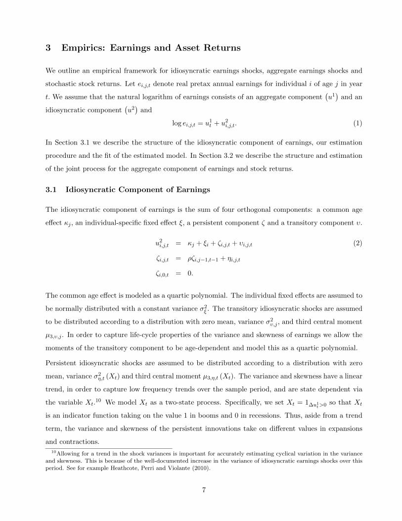
3.1 Idiosyncratic Component of Earnings
The idiosyncratic component of earnings is the sum of four orthogonal components: a common age
effect κj , an individual-specific fixed effect ξ, a persistent component ζ and a transitory component υ.
u2i,j,t = κj + ξi + ζi,j,t + υi,j,t (2)
ζi,j,t = ρζi,j−1,t−1 + ηi,j,t
ζi,0,t = 0.
The common age effect is modeled as a quartic polynomial. The individual fixed effects are assumed to
be normally distributed with a constant variance σ2ξ . The transitory idiosyncratic shocks are assumed
to be distributed according to a distribution with zero mean, variance σ2υ,j , and third central moment
µ3,υ,j . In order to capture life-cycle properties of the variance and skewness of earnings we allow the
moments of the transitory component to be age-dependent and model this as a quartic polynomial.
Persistent idiosyncratic shocks are assumed to be distributed according to a distribution with zero
mean, variance σ2η,t (Xt) and third central moment µ3,η,t (Xt). The variance and skewness have a linear
trend, in order to capture low frequency trends over the sample period, and are state dependent via
the variable Xt.10 We model Xt as a two-state process. Specifically, we set Xt = 1∆u1t>0 so that Xt
is an indicator function taking on the value 1 in booms and 0 in recessions. Thus, aside from a trend
term, the variance and skewness of the persistent innovations take on different values in expansions
and contractions.
10Allowing for a trend in the shock variances is important for accurately estimating cyclical variation in the varianceand skewness. This is because of the well-documented increase in the variance of idiosyncratic earnings shocks over thisperiod. See for example Heathcote, Perri and Violante (2010).
7
We estimate the idiosyncratic earnings process using data on male annual labor earnings from the
Panel Study of Income Dynamics (PSID) from 1967 to 1996.11 We focus on male heads of households
between ages 22 and 60 with real annual earnings of at least $1, 000. Our measure of annual gross
labor earnings includes pre-tax wages and salaries from all jobs, plus commission, tips, bonuses and
overtime, as well as the labor part of income from self-employment. Labor earnings are inflated to
2008 dollars using the CPI All Urban series. We also consider two sub-samples. Individuals with 12
or fewer years of education are included in the High School sub-sample, while those with at least 16
years or a Bachelor’s degree are included in the College sub-sample.
Estimation is done in two stages. In the first stage we estimate κj by regressing log real annual
earnings on a quartic polynomial in age and a full set of year dummies. This is done separately for
the three education samples. On the basis of the first-stage results for the PSID, and related results
for the Current Population Survey data and NIPA data, we set the contraction years over the time
interval 1967-1996 to be 1970, 1974-5, 1979-82, 1989-91 and 1993.
Residuals from this first-stage regression are then used to estimate the remaining parameters of the
individual earnings equation:(ρ, σ2
ξ , σ2η,t(Xt), µ3,η,t(Xt), σ
2ν,j , µ3,ν,j
). A GMM estimator is then used
to estimate the parameters, using the full set of second and third-order autocovariances as moments.12
The estimated process delivers a good fit to the variance and third central moment of the earnings
distribution as a function of both age and time. The fit of these and other moments for the full sample
is displayed in Figure 2. Corresponding results for the College and High School samples are contained
in the Appendix.
We highlight three findings from Table 1. First, transitory shocks are left skewed for the full sample
and the college sample. Left skewness is needed to match the left skewness of the first-stage residuals
as documented in Figure 2. Guvenen, Ozkan and Song (2014) document that male earnings growth
rates are left skewed in administrative data. Second, the variance and left skewness of persistent
shocks is higher in recessions than in booms. Consistent with the findings in Storesletten, Telmer and
Yaron (2004), there is evidence for counter-cyclical variance even when the framework is generalized
to account for skewness and a time trend. However, the cyclical variation that we estimate is less
11After 1996 the PSID was converted into a biannual survey.12When computing the auto covariance function, individuals are grouped into 5-year age cells so that when calculating
covariances at age j, individuals aged j ∈ [j − 2, j + 2] are used. Only cells with at least 30 observations are retained.The moments are weighted by n0.5
j,t,l where nj,t,l is the number of observations used to calculate the covariance at lag lin year t for age j. The maximum lag length is l = 10. Individuals aged 22 to 60 are used to construct the empiricalauto-covariance functions. This means that variances, covariance and third moments from ages 24 to 58 are effectivelyused in the estimation. Standard errors are calculated by bootstrap with 39 repetitions, thus accounting for estimationerror induced by the first-stage estimation.
8
dramatic than their findings. Third, the autoregression parameter ρ is higher for the full sample
and the college sample compared to the high school sample. Thus, persistent innovations of a given
magnitude will be of greater proportional importance for those with a college than a high school
education.
The parameter estimates are broadly consistent with those from related specifications (that do not
account for skewness), that have been estimated elsewhere in the literature and summarized in Meghir
and Pistaferri (2010).13 We note that our estimate of the variance of the transitory component is
approximately 0.1 larger than what has been estimated by others (see for example, Guvenen (2009)).
The source of this difference is due entirely to our broader sample selection. Since it is likely that a
substantial fraction of this variance is due to measurement error, we make an adjustment when using
these estimates as parameters in the structural model.14
3.2 Aggregate Component of Earnings and Stock Returns
Our benchmark model is a standard, first-order VAR for ∆yt =(
∆u1t logRst
)′. The error term εt
is a vector of zero mean IID random variables with covariance matrix Σ.
∆yt = γ + Γ∆yt−1 + εt (3)
We estimate (3) using data on male annual labor earnings from the the Current Population Survey
(CPS) from 1967 to 2008. Our sample selection criteria and definition of earnings are the same as
those used for the PSID, descibed in section 3.1. We construct an empirical counterpart to u1t by
estimating a median regression (Least Absolute Deviations) of earnings on a full set of age and time
dummies. We use a median regression rather than OLS since it is more robust to the effects of changes
in top coding in the CPS over our sample period. We use the estimates of u1t from our CPS sample,
rather than corresponding estimates from the PSID, as input to the estimation because CPS data has
both a longer time dimension and a larger cross-section sample each year compared to PSID data.
13Our model is estimated using data on log earnings levels. Estimation using data on log earnings growth rates wouldyield larger estimates of the persistent or permanent shocks. See Heathcote et al. (2010) for a discussion of this issue.We favor the estimation in levels since it allows us to accurately capture the age profile of the cross-sectional variance ofearnings.
14Using indirect inference on a structural model of consumption and savings behavior, Guvenen and Smith (2011)estimate that the variance of measurement error in male log annual earnings is around 0.02-0.025. Using a validationstudy of the PSID, French (2004) concludes that the variance of measurement error in the PSID is around 0.01. However,both of their samples are substantially more selected than ours, with a cross-sectional variance about 0.1 lower. Assumingthat half of this additional variance is due to measurement error, would suggest that around 0.05-0.06 of the estimatedtransitory variance is measurement error. Accordingly, we adjust our estimates of the variance σ2
ν,j down by 1/3 at allages. We adjust the third central moment at each age so that the coefficient of skewness, µ3,ν,j/σ
3ν,j remains unchanged
after adjusting the demoninator.
9
Data on equity and bond returns are annual returns. Equity returns are based on a value-weighted
portfolio of all NYSE, AMEX and NASDAQ stocks including dividends. Bond returns are based on
1-month Treasury bill returns.15 Real returns are calculated by adjusting for realized inflation using
the CPI All Urban series.
Table 2 reports the estimation results. The parameter estimates reveal a moderate degree of persistence
in aggregate earnings growth. The covariance between innovations to earnings growth and innovations
to stock returns is positive in all models. Thus, the estimated models imply a positive conditional
correlation between earnings growth and stock returns. This is one feature, among others, that will
later produce a positive conditional correlation between stock and human capital returns and a positive
stock component of the value of human capital.
The implied steady-state dynamics are reported in Table 3. The estimated model matches the observed
correlation structure well. When we input the estimated process into our economic model, we adjust
the constants (γ1, γ2) estimated in Table 2 so that all models produce in steady state E[logRs] = .041
and E[∆u1] = 0. This facilitates comparisons of human capital value and return properties across
models.
In Appendix A.3 we consider a generalization of (3). The generalization allows us to address the
possibility that earnings u1t and a process generating log stock returns are cointegrated. We assume
that yt =(u1t Pt
)′follows a p-th order VAR, where Pt is a process generating stock returns
(i.e. ∆Pt = logRst ). We show that this VAR can be written as a Vector Error Correction Mechanism
(VECM), a useful tool in the cointegration literature. We present lag order selection tests that suggest
the presence of two lags, i.e. p = 2. We also present tests of the cointegrating rank of this system. We
interpret these test findings as providing only weak evidence for cointegration. This leads us to adopt
(3) as the benchmark process. However, since these tests may all have relatively little power given the
short time series, we also estimate the model with cointegration and assess their implications within
the portfolio choice model.
4 The Benchmark Model
We now use the theoretical framework and the empirical results to quantify the value and return to
human capital. The benchmark model has two financial assets. Asset i = 1 is riskless and asset i = 2
is risky. The agent cannot go short on either financial asset. Initial resources at age j = 1 are denoted
15All returns come from Kenneth French’s data archive. We restrict attention to the period 1967-2008 since this is theperiod that the CPS earnings data covers.
10
by x which describes the sum of initial earnings and financial wealth.
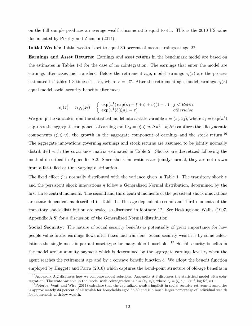
We group the variables from the statistical model into a state variable z = (z1, z2), where z1 = exp(u1)
captures the aggregate component of earnings and z2 = (ξ, ζ, υ,∆u1, logRs) captures the idiosyncratic
components (ξ, ζ, υ), the growth in the aggregate component of earnings and the stock return.16
The aggregate innovations governing earnings and stock returns are assumed to be jointly normally
distributed with the covariance matrix estimated in Table 2. Shocks are discretized following the
method described in Appendix A.2. Since shock innovations are jointly normal, they are not drawn
from a fat-tailed or time varying distribution.
The fixed effect ξ is normally distributed with the variance given in Table 1. The transitory shock υ
and the persistent shock innovations η follow a Generalized Normal distribution, determined by the
first three central moments. The second and third central moments of the persistent shock innovations
are state dependent as described in Table 1. The age-dependent second and third moments of the
transitory shock distribution are scaled as discussed in footnote 12. See Hosking and Wallis (1997,
Appendix A.8) for a discussion of the Generalized Normal distribution.
Social Security: The nature of social security benefits is potentially of great importance for how
people value future earnings flows after taxes and transfers. Social security wealth is by some calcu-
lations the single most important asset type for many older households.17 Social security benefits in
the model are an annuity payment which is determined by the aggregate earnings level z1 when the
agent reaches the retirement age and by a concave benefit function b. We adopt the benefit function
employed by Huggett and Parra (2010) which captures the bend-point structure of old-age benefits in
16Appendix A.2 discusses how we compute model solutions. Appendix A.3 discusses the statistical model with coin-tegration. The state variable in the model with cointegration is z = (z1, z2), where z2 = (ξ, ζ, υ,∆u1, logRs, w).
17Poterba, Venti and Wise (2011) calculate that the capitalized wealth implicit in social security retirement annuitiesis approximately 33 percent of all wealth for households aged 65-69 and is a much larger percentage of individual wealthfor households with low wealth.
12
the U.S. social security system. We employ the computationally-useful assumption that the benefit
function applies only to an agent’s idiosyncratic fixed effect rather than to an average of the agent’s
past earnings as in the U.S. system. Thus, the model benefit is risky after entering the labor market
only because the aggregate component of earnings at the time of retirement is risky. Old-age benefit
payments in the U.S. system are indexed to average economy-wide earnings when an individual hits
age 60.18 This is captured within the model by the fact that benefits are proportional to z1 ≡ exp(u1).
Properties of the benchmark model are displayed in Figure 3. It is constructed by simulating many
shock histories, calculating decisions along these histories and then taking averages at each age. Figure
3 shows that mean consumption, wealth and earnings net of taxes and transfers are hump shaped.
Financial wealth is exhausted before the end of life whereupon agents live off social security.
Equity participation rates in Figure 3 are above US values at all ages for all the risk aversion values
we analyze. Participation rates are calculated among agents with strictly positive financial assets as
is done in the literature. Chang et al. (2015) provide a useful review of findings in the literature
and document properties in data from the Survey of Consumer Finances (SCF). They find an average
participation rate of 55 percent in the SCF 1998-2007 for risky financial assets that include stock,
trusts, mutual funds and retirement accounts with exposure to risky assets. They find a hump-shaped
participation rate with age where the rate is roughly 30 percent within the 21-25 age group. Equity
participation rates in the model are just as high or higher at all ages as the patterns in Figure 3 when
we analyze constant-relative-risk-aversion (CRRA) preferences for CRRA values ranging from 1 to 6.
The results summarized above lead us to conclude that the benchmark model is far away from produc-
ing the low equity partcipation rates early in the working lifetime found in US data. This holds for a
wide range of preference parameter configurations. Thus, we provide support for one view within the
portfolio literature: the explanation of these portfolio facts is likely to rest on model properties beyond
those encompassed by enriching the Samuelson (1969) model with empirically realistic earnings and
financial asset return properties. This negative view is based on the robust result that the stock share
of the value of human capital is not particularly large when earnings and asset returns are driven by
a process estimated from US data.
5 Human Capital Values and Returns: Benchmark Model
We report properties of the benchmark model based on the high school and the college subsamples.
Results for the full sample are typically between the results for these education groups.
18See the Social Security Handbook (2012, Ch. 7).
13
5.1 Human Capital Values
Figure 4 plots the value of human capital in the benchmark model and a decomposition of this value.
The mean value of human capital over the lifetime is hump shaped and is lower for higher values of
the risk aversion coefficient.19 For comparison purposes, we also plot the value of human capital that
would be implied by discounting future earnings at the risk-free rate. We label this the naive value.
Our notion of value lies far below the naive value. This occurs because of negative covariation between
an agent’s stochastic discount factor and earnings and because agents are sometimes on the corner of
the risk-free asset choice. Corner solutions occur more frequently early in life for college agents than
for high school agents due to differences in the mean earnings profile. When an agent is on the corner,
then the agent discounts certain future earnings at more than the risk-free rate.
We now decompose human capital values into a bond, a stock and a residual-value component. This
follows the method discussed in section 2. To do so, we project next period’s human capital payout
vj+1 + ej+1 onto the space of conditional gross bond and stock returns.20
vj = E[mj,j+1(vj+1 + ej+1)|zj ] = E[mj,j+1(∑i∈I
αijRij+1 + εj+1)|zj ]
Figure 4 calculates the value of the bond and stock components αbjE[mj,j+1Rbj+1|zj ] and αsjE[mj,j+1R
sj+1|zj ]
as well as the value of the orthogonal component E[mj,j+1εj+1|zj ]. It then expresses these values as
a fraction of the value of human capital at each age and then averages these ratios across the states
that occur at each age. Appendix A.2 describes our methods for computing the projection coefficients
in the value decomposition and each assets share in the value of human capital. The bond component
averages more than 80 percent of the value of human capital. This holds for both education groups
and for a range of risk-aversion parameters.
Figure 4 shows that the stock component of the value of human capital is positive on average. It
averages below 35 percent at all ages for high school agents and below 20 percent for college agents for
a wide range of risk-aversion parameters. The stock component is positive, at a given age and state,
provided that the sum of next period’s earnings and human capital value covaries positively with the
return to stock, conditional on this period’s state. Our empirical work, as summarized in Table 2,
directly relates to the conditional comovement of earnings and stock returns since cov(ε1,t, ε2,t) > 0
in all the estimated models.19Figure 3(a)-(b) are constructed by first computing human capital values at each age as a function of the state. We
then calculate the sample average of the value at each age, conditional on survival, by simulating many realizations ofthe state variable over the lifetime. Computational methods are described in the Appendix.
20The Appendix describes our methods for computing the projection coefficients αi in the value decomposition.
14
The orthogonal component has a large negative value early in the lifetime. Given that the orthogonal
component has a zero mean, this is due to strong negative covariation between the orthogonal compo-
nent and the stochastic discount factor early in life. This occurs, for example, because consumption
and future utility are increasing in the realization of the persistent idiosyncratic earnings shock, other
things equal. Section 6 will show that the persistent shock component is particularly important early
in life in lowering human capital values. Such a shock has many periods over which it impacts future
earnings.
While it may seem plausible that the value of human capital is largely bond-like during retirement,
it is useful to understand why it is not always 100 percent bond-like. If a retired agent will in all
future date-events end up holding positive bonds, then the decomposition will indeed calculate that
this agent’s human capital in retirement is 100 percent bond-like as social security annuity payments
in the model are riskless after retirement. However, if an agent hits the corner of the bond decision in
the future under some sequence of risky stock returns, then this is not true. The mean of the agent’s
stochastic discount factor will be less than the inverse of the gross risk-free rate in such an event.
Thus, the agent discounts future social security transfers at greater than the risk-free rate beyond this
date. The value of these transfers at earlier dates takes on a positive stock component provided that
a corner solution is induced by low stock return realizations. In summary, while the value of human
capital is mostly bond-like in retirement, it is not 100 percent bonds because agents run down financial
assets, hit a corner solution on the holdings of the risk-free asset and live off social security transfers.
5.2 Human Capital Returns
Figure 5 plots properties of human capital returns. Mean returns are very large early in the working
lifetime. To understand what drives the mean human capital returns, it is useful to return to the
main ideas used in the value decomposition. The first equation below decomposes gross returns by
decomposing the future payout into a bond, a stock and an orthogonal component. The second
equation shows that the conditional mean human capital return always equals the weighted sum of
the conditional mean of the bond and stock return.21
Rhj+1 ≡vj+1 + ej+1
vj=αbjR
bj+1 + αsjR
sj+1 + ε
vj
E[Rhj+1|zj ] =αbjvjE[Rbj+1|zj ] +
αsjvjE[Rsj+1|zj ]
21The orthogonal component drops out as, with a risk-free asset, the mean of the orthogonal component is zero.
15
The weights on the bond and stock return do not always sum to one. When the agent’s Euler equation
for both stock and bonds hold with equality, then these weights will sum to more than one exactly
when the value of the orthogonal component is negative.22 The value of the orthogonal component
of human capital payouts is negative early in the working lifetime. Human capital returns can vastly
exceed a convex combination of stock and bond returns when the weights sum to more than one.
The mean return to human capital is near the risk-free rate immediately after retirement but sub-
sequently increases. The high return towards the end of the lifetime might at first seem odd.
This should not be surprising, however, as in the penultimate period vJ−1 = E[mJ−1,JeJ ] and
1 = E[mJ−1,JeJ/vJ−1]. As the payment eJ , conditional on surviving to the last period, is certain,
the return is RhJ = eJ/vJ−1 = 1/E[mJ−1,J ]. Thus, the return equals the risk-free bond rate when the
agent is off the corner (i.e. RhJ = 1/E[mJ−1,J ] = Rb) but can exceed the risk-free rate when the agent
is on the corner (i.e. RhJ = 1/E[mJ−1,J ] ≥ Rb). Towards the end of the lifetime an increasing fraction
of agents in the model are on this corner consistent with the wealth profile in Figure 3.
The positive correlation between human capital returns and stock returns in Figure 5 is based in
part on two properties. First, innovations to the aggregate component of earnings growth and to
stock returns are positively correlated. This implies that the component of human capital returns
related directly to the earnings payout next period covaries positively with stock returns. Second, the
old-age transfer benefit formula in the benchmark model is proportional to the aggregate component
of earnings at the retirement age. The U.S. social security system has a similar feature as old-age
benefits are proportional to a measure of average earnings in the economy when the worker turns age
60, other things equal.
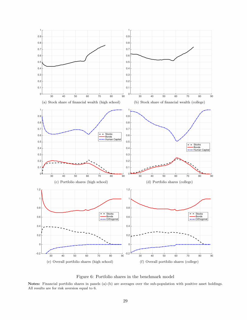
5.3 Portfolio Allocation
Figure 6 describes portfolio allocation based on financial wealth and on overall wealth (i.e. financial
plus human wealth). Figure 6 (a)-(b) plots the average share of financial wealth in stock among those
holding positive assets. The high-school agents have a lower average stock share than the college
agents over most of the working lifetime.
Figure 6 provides two descriptions of portfolio allocation based on overall wealth. First, consider how
overall wealth is split between stock, bonds and the value of human capital. For both the high school
and college groups, human capital is the largest component of wealth on average at each age. This
22In this case, vj = E[mj+1(vj+1 + ej+1)] = αbj +αsj +E[mj+1εj+1] and E[mj+1εj+1] < 0 imply αbj/vj +αsj/vj > 1. Ofcourse, the weights for decomposing returns can and do sum to more than one even when Euler equations do not holdwith equality.
16
holds despite the fact that the value of human capital to the individual is far below the naive value
over the working lifetime.
Figure 6 also divides overall wealth into a stock, bond and an orthogonal value component. The
stock component is then the sum of stock directly held in the financial wealth portfolio and the stock
position embodied in the value of human capital based on the analysis in section 5.1. We find that the
bond share of overall wealth exceeds the stock share at all ages. The stock share for the college group
averages between 20 to 30 percent over the working lifetime, whereas for high school it average between
20 to 40 percent over the working lifetime. The overall stock share early in life is largely determined
by the decomposition analysis presented earlier in Figure 4. This is because financial assets are small
in value compared to the value of human capital and negative positions in either financial asset are
not allowed.
It is perhaps useful to view the average stock shares in Figure 6 (e)-(f) from the perspective of the stock
share formula 1α
E[Rx]V ar(Rx)
.= 1
6.05.04
.= .21 holding in the Samuelson (1969) model. In this formula α is the
relative-risk-aversion coefficient and we plug in the mean and the variance of the excess return Rx on
equity.23 While backgroud risk, correlated returns, multiple-period horizons and corner solutions are
present in the benchmark model underlying Figure 6 and invalidate this simple formula (see Gollier
(2002)), it is interesting to see that average overall stock shares in Figure 6 are not wildly at odds
with this formula.
6 Discussion: Robustness and Drivers
This section determines the robustness and drivers of two findings: (1) the value of human capital is
far below the naive value and (2) the stock component of human capital averages less than 35 percent
of the value of human capital at all ages.
6.1 Value of Human Capital
What drives the value of human capital to be substantially below the naive value? To answer this
question, we consider a number of perturbations of the benchmark model. For each perturbation, we
recalculate human capital values and then plot the results. The benchmark model is the model in
Table 4 that sets risk aversion to α = 6 and that sets earnings to the process without cointegration
estimated for the full sample.
23The mean and variance are calculated, based on a lognormal distribution, using the mean and variance of log returnsfrom US data in Table 3.
17
We first consider perturbations that help agents to better smooth consumption. Intuitively, such
perturbations lessen the negative covariation between the stochastic discount factor and earnings.
One perturbation starts agents off with an initial wealth of 1 times mean earnings at age 22 rather
than the benchmark value of 30 percent of mean earnings. The other perturbations allow agents
to hold negative balances in the risk-free asset up to 1.0 times mean earnings or up to the natural
borrowing limit. Figure 7 shows that while all perturbations increase the human capital value early
in life, values remain well below the naive value.
Next we examine the extent to which transitory or persistent idiosyncratic shocks are key drivers.
First, we eliminate transitory or persistent shocks. Figure 7 shows that eliminating transitory shocks
increases human capital values. However, the quantitative effects are small compared to the massive
impact of eliminating persistent idiosyncratic shocks. Eliminating persistent shocks produces more
than a tripling of the value of human capital early in life. Lastly, we impose that persistent shocks
have no skewness and no cyclical variation in variance or skewness. Figure 7 shows that this increases
human capital values and that its effect is more powerful than eliminating transitory shocks. This
foreshadows the importance of skewness as a driver of the stock component of human capital values
that we find in the next subsection. We note that for each of these three changes we re-estimate the
model with the new restrictions imposed.
We examine the effect of altering the preference parameter γ, while keeping relative risk aversion
fixed. The value of 1/γ controls the intertemporal elasticity of substitution (IES). Figure 7 shows that
increasing the IES to 2 increases the human capital value slightly, whereas decreasing the IES to 0.5
reduces the value of human capital. Neither change alters the finding that human capital values are
substantially below naive values.
6.2 Stock Share of Human Capital Values
What drives the magnitude of the stock share of human capital values? We answer this question by
analyzing four perturbations of the benchmark model. We (i) vary the borrowing constraint, (ii) vary
the IES and/or risk aversion, (iii) eliminate the cyclical changes in persistent idiosyncratic shocks
and/or eliminate the left-skewness in these shocks and (iv) allow cointegration.
Figure 8 shows the results. Raising the IES to 2 lowers the stock component slightly whereas lowering
the IES to 0.5 raises the stock share slightly. Allowing borrowing up to one times mean earnings
has almost no visible impact on the stock share and we therefore do not display this result. Figure
8(b) analyzes what happens when we increase risk aversion α and reduce the IES measured by 1/γ at
18
the same time by setting γ = α, effectively imposing CRRA preferences. The stock share rises as α
increases.
Next we eliminate skewness and/or eliminate the cyclical variation in shock distributions. The case
of no skewness means that the generalized normal distribution analyzed in the benchmark model is
replaced by the normal distribution. In all cases, we re-estimate the idiosyncratic shock process under
the new restrictions to best match data moments.
Figure 8 shows that eliminating left-skewness and eliminating cyclicality decreases the stock share of
human capital values. This could be stated more positively if one took the benchmark model to be the
model with no skewness and no cyclical changes in idiosyncratic shocks. Using that model as a bench-
mark, implies that allowing left-skewed shocks and allowing the distribution of such shocks to vary
cyclically increases the stock share of human capital. The incremental effect of adding left-skewness
is substantially larger than adding cyclical variation in a distribution displaying no skewness.24 Thus,
we find that skewness is a quantitatively important factor that increases the stock share of human
capital values and lowers human capital values.
We now consider statistical models that allow the aggregate component of earnings to be cointegrated
with stock returns. Appendix A.3 presents a time series model that allows for cointegration and
that nests the benchmark time series model from section 3.2 as a special case. Table A.4 and Table
A.5 present parameter estimates and steady state properties of the estimated model. Some intuition
for why cointegration may matter is that over long horizons aggregate shock histories with high
realizations for the aggregate component of earnings will be associated with histories of high stock
returns. Correspondingly, low earnings histories will be associated with histories of low stock returns.
Cointegration implies that two series do not drift apart. Such a process could lead an individual’s
earnings far into the future to take on stock-like features.
Figure 8 addresses whether cointegration is important for the magnitude of the stock share of human
wealth. First, we compare the benchmark model and the model allowing cointegration when both
are estimated using CPS 1967-2008 data for the full sample. Allowing cointegration slightly decreases
the stock share of human capital values. One might be skeptical that a cointegrated relationship
can be precisely estimated over a short time period. For this reason, we repeat the analysis using
an aggregate measure of earnings growth to proxy male earnings growth. We use NIPA 1929-2009
data on aggregate wages and salaries and divide this by the labor force to get average earnings. We
24Storesletten, Telmer and Yaron (2007) and Lynch and Tan (2011) argue that adding counter-cyclical variation inthe variance of idiosncratic shocks, in a model without skewness, reduces the stock share of the financial asset portfolio.
19
re-estimate both models using data over the period 1929-2009.25 Figure 8 shows that the stock share
increases somewhat using NIPA data when these estimated models are incorporated into the economic
model. However, allowing cointegration does not significantly alter the stock share compared to the
case of no cointegration, given the new data.
In summary, Figure 8 shows that two changes to the benchmark model produce a larger stock share.
These are to decrease the IES to values below 1 and to re-estimate the model using NIPA data over a
longer time period. We also find that skewness is an important driver of the stock share. Abstracting
from skewness implies a much smaller stock share of human capital.26 While one may conjecture that
allowing cointegration may substantially increase the stock share of the value of human capital, we do
not find support for this when the models are estimated using the same data set.
This last finding may seem surprising in light of the work of Benzoni et al. (2007). The main focus
of their work is to examine how cointegration affects portfolio choice as a single parameter κ that
controls the strength of adjustment in the cointegrating relationship increases. Stock holding in the
financial asset portfolio is zero early in life in their model for a sufficiently large value of κ, when the
relative-risk aversion coefficient is set to equal 5. For the parameter configuration that they highlight,
the stock component of the value of human capital is 50 percent at age 20 and remains at 50 percent
throughout the first half of the working lifetime.
Our model differs from their work in a number of dimensions. For example, we model social security
benefits, allow idiosyncratic shocks to be drawn from a skewed distribution and allow for cyclical
changes in idiosyncratic shocks. They abstract from all of these features. In addition, the methodology
differs. While we estimate the idiosyncratic and aggregate shock structure, they roughly calibrate a
cointegrated aggregate process governing stock returns and the aggregate component of earnings.
To make contact with Benzoni et al. (2007), we simply take the calibrated aggregate process from their
work and substitute it into our model. Their calibrated process has the discrete-time approximation
of the form indicated below. We take as given their parameter value for κ = 0.15 and their values
governing the variance-covariance structure of the shock terms (ε1, ε2, ε3). We adjust the constant
terms (γ1, γ2) so that E[logR] = .041 and E[∆u] = 0 in all models.27
25Table A.5 in Appendix A.3 presents steady state properties of these different models.26One might conjecture that increasing the mean growth rate E[∆u1
t ] from the sample average of zero might matter.Increasing this mean from zero to 1 or 2 percent substantially increases individual human capital values while leavingthe stock share essentially unchanged in the benchmark model.
27Appendix A.3 shows how we go from their continuous-time formulation to the discrete-time model and computessteady-state properties. The Benzoni et al. (2007) process produces an unconditional standard deviation of SD(∆ut) =0.069 which is more than twice the values that we calculate in US earnings data as documented in Table A.5 and TableA.6.
20
∆ut+1
logRt+1
wt+1
=
γ1
γ2
0
+
0 0 −κ0 0 00 0 1− κ
∆utlogRtwt
+
ε1,t+1
ε2,t+1
ε3,t+1
(4)
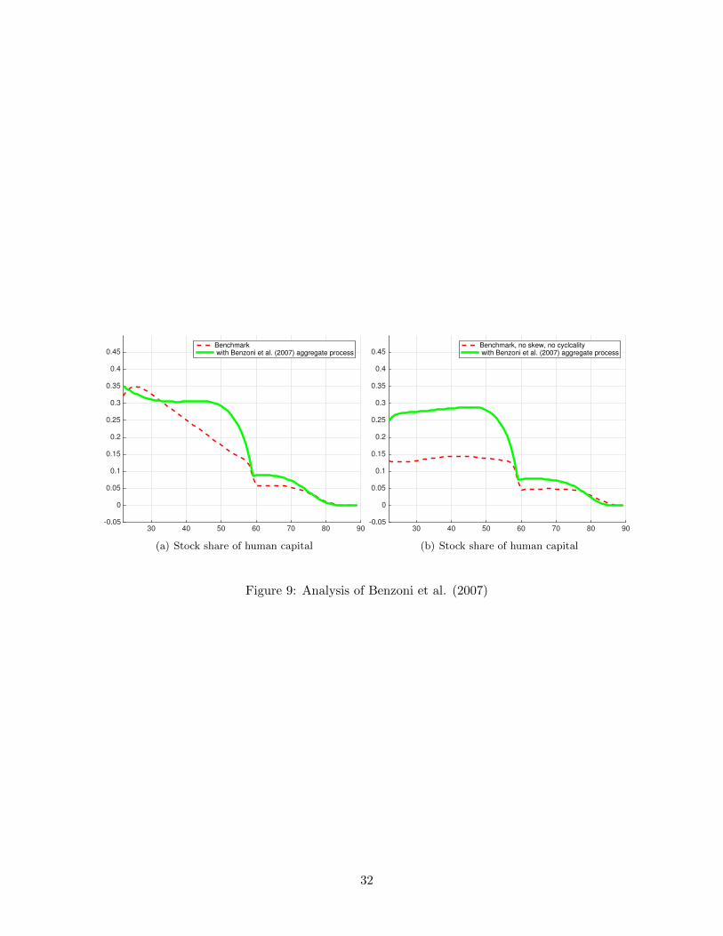
Figure 9(a) compares the benchmark model (without cointegration) from this section to the model
that results from replacing the aggregate dynamics with the Benzoni et al. (2007) process featuring
cointegration. When inserted into our framework, the Benzoni et al. (2007) process produces a stock
share that is well below the 50 percent value that they highlight.
Figure 9(b) considers a different comparison. The benchmark model is now modified to exclude
skewness and cyclical variation in idiosyncratic risk, but is still estimated to best match data. We
then insert the Benzoni et al. (2007) process into this model. Figure 9(b) shows that once again both
models produce a stock share that is well below 50 percent over the lifetime. The results in Figure 9
are essentially unchanged if the mean log earnings growth rate is increased to equal 1 percent in all
the models rather than the benchmark value of zero.
7 Conclusion
Our analysis highlights two main properties of human capital values based on an analysis of U.S. data
on males earnings and financial asset returns: (1) the value of human capital is far below the value
implied by discounting future earnings at the risk-free rate and (2) the stock component of the value
of human capital averages less than 35 percent at each age over the working lifetime. These properties
hold for (i) different educational groups, (ii) a wide range of parameters characterizing risk aversion
and intertemporal substitution, (iii) a range of assumptions on borrowing constraints and (iv) two
different statistical models for earnings estimated using male earnings data.
We investigate the main drivers of these two findings. Persistent idiosyncratic shocks and the left
skewness of idiosyncratic shocks are two key drivers of low human capital values. In our model frame-
work, an agent’s stochastic discount factor falls for larger realizations of idiosyncratic shocks, other
things equal. A number of model features lead to a positive stock component of the value of human
capital including (i) social security benefits linked to average earnings, (ii) positive conditional correla-
tion between the aggregate component of earnings and stock returns and (iii) left-skewed idiosyncratic
earnings shocks. We provide support for these features in US data. We do not find much support
in US data for the idea that cointegration between the aggregate component of earnings and stock
returns is a key factor driving the size of the stock share of the value of human capital.
21
References
Alvarez, F. and U. Jermann (2004), Using Asset Prices to Measure the Cost of Business Cycles,Journal of Political Economy, 112, 1223-56.
Becker, G. (1975), Human Capital, Second Edition, National Bureau of Economic Research.
Benzoni, L., Collin-Dufresne, P. and R. Goldstein (2007), Portfolio Choice over the Life-Cyclewhen the Stock and Labor Markets are Cointegrated, Journal of Finance, 62, 2123-67.
Chang, Y., Hong, J. and M. Karabarbounis (2015), Labor-Market Uncertainty and PortfolioChoice Puzzles, Federal Reserve Bank of Richmond Working Paper 14-13R.
Coco, J. (2005), Portfolio Choice in the Presence of Housing, The Review of Financial Studies,18, 353-67.
Coco, J., Gomes, F. and P. Maenhout (2005), Consumption and Portfolio Choice over the LifeCycle, Review of Financial Studies, 18, 491-533.
Constantinides, G. and D. Duffie (1996), Asset Pricing with Heterogeneous Consumers, Journalof Political Economy, 104, 219-40.
Dublin, L. and A. Lotka (1930), The Money Value of a Man, The Ronald Press Company.
Epstein, L. and S. Zin (1991), Substitution, Risk Aversion and the Temporal Behavior of Con-sumption and Asset Returns: An Empirical Analysis, Journal of Political Economy, 99, 263-86.
Farr, W. (1853), The Income and Property Tax, Journal of the Statistical Society of London,16, 1-44.
French, E. (2004), The Labor Supply Response to (Mismeasured but) Predictable Wage Changes,Review of Economics and Statistics, 86(2), 602-613.
Gollier, C. (2002), What Does Classical Theory Have to Say about Household Portfolios?, inHousehold Portfolios, edited L. Guiso, M. Haliassos and T. Jappelli, The MIT Press.
Gomes and Michaelides (2005), Optimal Life-Cycle Asset Allocation: Understanding the Em-pirical Evidence, Journal of Finance, 60, 869-904.
Graham, J. and R. Webb (1979), Stocks and Depreciation of Human Capital: New Evidencefrom a Present-Value Perspective, Review of Income and Wealth, 25, 209- 24.
Guvenen, F. (2009), An Empirical Investigation of Labor Income Processes, Review of EconomicDynamics, 12(1), 58-79.
Guvenen, F. and A. Smith (2011), Inferring Labor Income Risk from Economic Choices: AnIndirect Inference Approach, manuscript.
Guvenen, F., Ozkan, S. and J. Song (2014), The Nature of Countercyclical Income Risk, Journalof Political Economy, 122, 621-60.
Haveman, R., Bershadker, A. and J. Schwabish (2003), Human Capital in the United Statesfrom 1975 to 2000: Patterns of Growth and Utilization, Upjohn Institute.
Heathcote, J., Perri, F. and G. Violante (2010), Unequal We Stand: An Empirical Analysis ofEconomic Inequality in the United States, Review of Economic Dynamics, 13(1), 15-51.
Hosking, J. and J. Wallis (1997), Regional Frequency Analysis, Cambridge University Press.
22
Huggett, M. and G. Kaplan (2011), Human Capital Values and Returns: Bounds Implied ByEarnings and Asset Returns Data, Journal of Economic Theory, 146, 897-919.
Huggett, M. and G. Kaplan (2012), The Money Value of a Man, NBER Working Paper 18066.
Huggett, M. and J.C. Parra (2010), How Well Does the U.S. Social Insurance System ProvideSocial Insurance?, Journal of Political Economy, 118, 76-112.
Johansen, S. (1995), Likelihood-Based Inference in Cointegrated Vector Autoregressive Models,Oxford University Press.
Jorgenson, D. and B. Fraumeni (1989), The Accumulation of Human and Nonhuman Capital,1948- 1984, in The Measurement of Saving, Investment and Wealth, R. Lipsey and H. Tice, eds.NBER Studies in Income and Wealth.
Lucas, R. (1978), Asset Prices in an Exchange Economy, Econometrica, 46, 1429- 45.
Lynch, A. and S. Tan (2011), Labor Income Dynamics at Business-Cycle Frequencies: Implica-tions for Portfolio Choice, Journal of Financial Economics, 101, 333-59.
Meghir, C. and L. Pistaferri (2010), Earnings, Consumption and Lifecycle Choices, NBER Work-ing Paper.
NCHS (1992), US Decennial Life Tables 1989-1991, Washington, DC: Hyattsville, Md.
Nerlove, M. (1975), Some Problems in the Use of Income-Contingent Loans for the Finance ofHigher Education, Journal of Political Economy, 83, 157-84.
Piketty, T. and G. Zucman (2014), Capital is Back: Wealth-Income Ratios in Rich Countries17002010, Quarterly Journal of Economics, 129, 1155-1210.
Poterba, J., Venti, S. and D. Wise (2011), The Composition and Drawdown of Wealth in Re-tirement?, Journal of Economic Perspectives, 25, 95-118.
Samuelson, P. (1969), Lifetime Portfolio Selection by Dynamic Stochastic Programming, Reviewof Economics and Statistics, 51, 239-46.
Social Security Handbook (2012), available http://www.ssa.gov.
Storesletten, K., Telmer, C. and A. Yaron (2004), Cyclical Dynamics in Idiosyncratic Labor-Market Risk, Journal of Political Economy, 112, 695-717.
Storesletten, K., Telmer, C. and A. Yaron (2007), Asset Pricing with Idiosyncratic Risk andOverlapping Generations, Review of Economic Dynamics, 10, 519-48.
Vissing-Jorgensen, A. and O. Attanasio (2003), Stock-Market Participation, Intertemporal Sub-stitution, and Risk-Aversion, American Economic Review Papers and Proceedings, 93, 383-91.
Weisbrod, B. (1961), The Valuation of Human Capital, Journal of Political Economy, 69, 425-36.
23
0 0.05 0.1 0.15 0.2 0.25 0.30
5
10
15
20
25
30
35
40
σ: st dev earnings shocks
Naive value
ρ = 1
ρ = 2
ρ = 4
(a) Value of human capital
0 0.05 0.1 0.15 0.2 0.25 0.30
5
10
15
20
25
30
35
40
45
σ: st dev earnings shocks
ρ = 1
ρ = 2
ρ = 4
(b) Mean return human capital (%)
0 0.05 0.1 0.15 0.2 0.25 0.30
100
200
300
400
500
600
σ: st dev earnings shocks
Marginal benefit (ρ = 2)
Total benefit (ρ = 2)
(c) Benefit of moving to a smooth consumption plan(%)
Figure 1: Human capital values and returns: a simple example
24
1965 1970 1975 1980 1985 1990 1995 20000.2
0.3
0.4
0.5
0.6
0.7
0.8
Data
Model
(a) Variance of log earnings by year
20 25 30 35 40 45 50 55 600.3
0.35
0.4
0.45
0.5
0.55
0.6
0.65
0.7
0.75
0.8
Data
Model
(b) Variance of log earnings by age
1965 1970 1975 1980 1985 1990 1995 2000−1
−0.9
−0.8
−0.7
−0.6
−0.5
−0.4
−0.3
−0.2
−0.1
0
Data
Model
(c) Third central moment of log earnings by year
20 25 30 35 40 45 50 55 60
−0.6
−0.5
−0.4
−0.3
−0.2
−0.1
0
Data
Model
(d) Third central moment of log earnings by age
0 2 4 6 8 100
0.05
0.1
0.15
0.2
0.25
0.3
0.35
0.4
Data
Model
(e) Average autocovariance function
Figure 2: Fit of estimated idiosyncratic earnings model for the full sample
Figure 3: Life-cycle profiles in the benchmark model
Notes: Left panels refer to high-school sub-sample, right panels refer to college sub-sample. The vertical scale in(a)-(b) is in units of 100,000 dollars in year 2008. Participation rates are conditional on having positive financial wealth.Equity shares are conditional on having positive equity.
26
30 40 50 60 70 80 900
5
10
15
20
25
30
35
40
Mean Naive Value
Mean Value: RA=4
Mean Value: RA=6
Mean Value: RA=10
(a) Human capital values (high school)
30 40 50 60 70 80 900
5
10
15
20
25
30
35
40
Mean Naive Value
Mean Value: RA=4
Mean Value: RA=6
Mean Value: RA=10
(b) Human capital values (college)
30 40 50 60 70 80 90
-0.2
0
0.2
0.4
0.6
0.8
1
1.2
Stock ComponentBond ComponentOrthogonal Component
(c) Decomposition (high school)
30 40 50 60 70 80 90
-0.2
0
0.2
0.4
0.6
0.8
1
1.2
Stock ComponentBond ComponentOrthogonal Component
(d) Decomposition (college)
Figure 4: Human capital values and a decomposition
Notes: The vertical scale in Figure 3 (a)-(b) is in units of 100,000 dollars in year 2008.
Notes: Financial portfolio shares in panels (a)-(b) are averages over the sub-population with positive asset holdings.All results are for risk aversion equal to 6.
(a) Human capital values (borrowing, initial wealth)
30 40 50 60 70 80 900
5
10
15
20
25
30
Naive ValueBenchmarkNo skewness and no cyclicality in shocksNo persistent shocksNo transitory shocks
(b) Human capital values (idiosyncratic risk)
30 40 50 60 70 80 900
5
10
15
20
25
30
Naive Value
Benchmark
IES=2
IES=0.5
(c) Human capital values (IES)
Figure 7: What drives the value of human capital?
Notes: In panel (a) “With borrowing (1x)” refers to the model that allows borrowing up to 1 times average annualearnings, and “With borrowing (NBL)” refers to model that allows borrowing up to the “Natural Borrowing Limits” i.e.limits that impose only that the agent must be able to repay his debt in all states of the world.
(d) Stock component of human capital (cointegration)
Figure 8: What drives the stock component of human capital?
Notes: When comparing different models estimated on the same data set or the same model estimated on different datasets, the constants in all models are reset so that E[∆uit] = 0 and E[logRst ] = 0.041 as previously noted in Table 3. Thebenchmark model is the model from Table 4 with α = 6 and without cointegration.
31
30 40 50 60 70 80 90-0.05
0
0.05
0.1
0.15
0.2
0.25
0.3
0.35
0.4
0.45Benchmark with Benzoni et al. (2007) aggregate process
(a) Stock share of human capital
30 40 50 60 70 80 90-0.05
0
0.05
0.1
0.15
0.2
0.25
0.3
0.35
0.4
0.45Benchmark, no skew, no cyclcality with Benzoni et al. (2007) aggregate process
(b) Stock share of human capital
Figure 9: Analysis of Benzoni et al. (2007)
32
Table 1: Parameter Estimates for the Idiosyncratic Earnings Process
Notes: Table shows average moments in the data, together with implied steady-state statistics from the correspondingestimated model. Data cover the period 1967-2008. When implementing the estimated processes in the structural model,we adjust the constants (γ1, γ2) estimated in Table 2 so that all models have E[logRst ] = 0.041 and E[∆u1
t ] = 0.
34
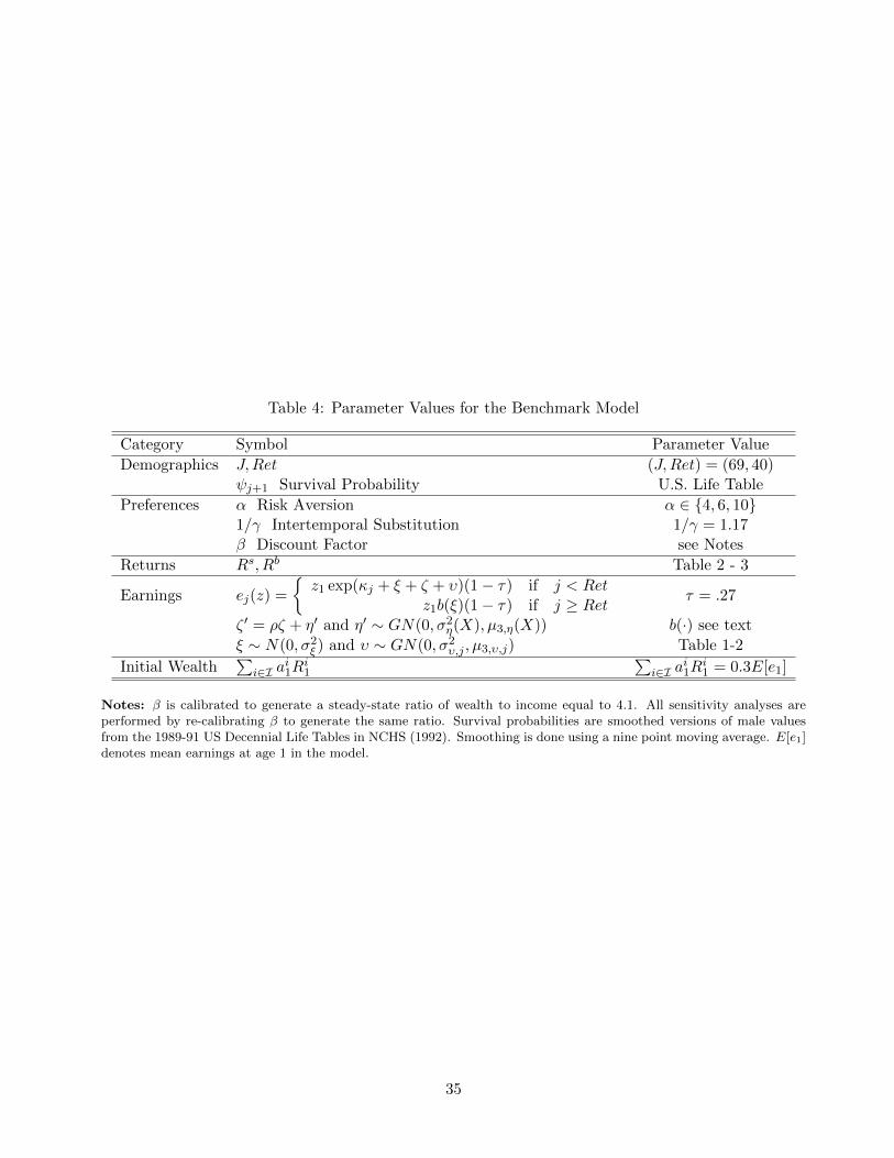
Table 4: Parameter Values for the Benchmark Model
Category Symbol Parameter Value
Demographics J,Ret (J,Ret) = (69, 40)ψj+1 Survival Probability U.S. Life Table
ζ ′ = ρζ + η′ and η′ ∼ GN(0, σ2η(X), µ3,η(X)) b(·) see text
ξ ∼ N(0, σ2ξ ) and υ ∼ GN(0, σ2
υ,j , µ3,υ,j) Table 1-2
Initial Wealth∑
i∈I ai1R
i1
∑i∈I a
i1R
i1 = 0.3E[e1]
Notes: β is calibrated to generate a steady-state ratio of wealth to income equal to 4.1. All sensitivity analyses areperformed by re-calibrating β to generate the same ratio. Survival probabilities are smoothed versions of male valuesfrom the 1989-91 US Decennial Life Tables in NCHS (1992). Smoothing is done using a nine point moving average. E[e1]denotes mean earnings at age 1 in the model.
35
A Appendix
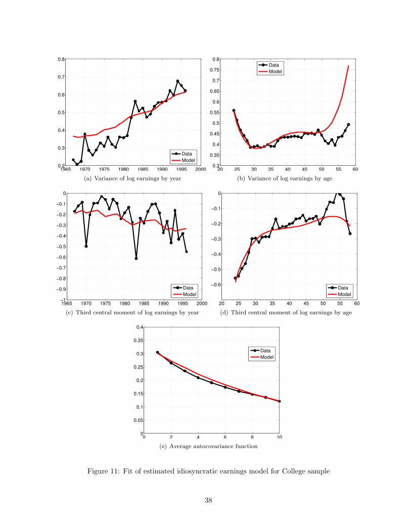
A.1 Model Fit
The fit of the earnings model for the high school and college samples is provided in Figure 10 and 11respectively.
A.2 Computation
This section describes our methods to compute solutions to the benchmark model and to computevalues and returns.
A.2.1 Value Function and Decision Rules
To compute the optimal value function V ∗j and optimal decision rules to the model in section 4,we employ the method of dynamic programming. This involves computing functions Vj solving theBellman equation (BE). Of course, the idea is that Vj = V ∗j . In stating Γj(x, z) in Bellman’s equation,we impose the restrictions from the original budget constraint Γj(x, z). We also use the fact thatshocks are Markovian so that the current shock, denoted z, rather than partial histories zj contain allrelevant information. We model the shock z = (z1, z2) as stated in section 4.
V ∗j (x, z) ≡ maxW (cj , F (U(cj+1, ..., cJ)), j) s.t. c ∈ Γj(x, z)
We compute solutions to Bellman’s equation only when the first component of the shock z = (z1, z2)takes the value z1 = 1. This is indicated below. To do so requires knowledge of Vj+1(x′, z′1, z
′2) at
all values of z′1. Lemma 1 below shows that V ∗j (λx, λz1, z2) = λV ∗j (x, z1, z2), ∀λ > 0 and thereforeV ∗j (x, z1, z2) = z1V
∗j ( xz1 , 1, z2). In the Algorithm described below, we make use of this key property.
In Lemma 1, Γ(x, z) is homogeneous provided c ∈ Γ(x, z)⇒ λc ∈ Γ(λx, λz),∀λ > 0.
Vj(x, 1, z2) = max(c,a1,a2)∈Γj(x,1,z2)
W (cj , F (Vj+1(x′, z′1, z′2)), j)
Lemma 1:
(i) Assume U is homothetic and Γ(x, z) is homogeneous. c∗ ∈ argmax U(c) : c ∈ Γ(x, z) impliesλc∗ ∈ argmax U(c) : c ∈ Γ(λx, λz),∀λ > 0.
(ii) In the benchmark model V ∗j (λx, λz1, z2) = λV ∗j (x, z1, z2), ∀λ > 0
Proof:
(i) obvious
(ii) Follows from Lemma 1(i) after noting two things. First, EZ preferences are homothetic and, infact, homogeneous of degree 1. Second, Γj(x, z) is homogeneous in (x, z1) for any fixed z2. This isimplied because the earnings function from the benchmark model is ej = z1gj(z2) and z′1 = z1fj+1(z′2),
36
1965 1970 1975 1980 1985 1990 1995 20000.2
0.3
0.4
0.5
0.6
0.7
0.8
Data
Model
(a) Variance of log earnings by year
20 25 30 35 40 45 50 55 600.3
0.35
0.4
0.45
0.5
0.55
0.6
0.65
0.7
0.75
0.8
Data
Model
(b) Variance of log earnings by age
1965 1970 1975 1980 1985 1990 1995 2000−1
−0.9
−0.8
−0.7
−0.6
−0.5
−0.4
−0.3
−0.2
−0.1
0
Data
Model
(c) Third central moment of log earnings by year
20 25 30 35 40 45 50 55 60
−0.6
−0.5
−0.4
−0.3
−0.2
−0.1
0
Data
Model
(d) Third central moment of log earnings by age
0 2 4 6 8 100
0.05
0.1
0.15
0.2
0.25
0.3
0.35
0.4
Data
Model
(e) Average autocovariance function
Figure 10: Fit of estimated idiosyncratic earnings model for High School sample
37
1965 1970 1975 1980 1985 1990 1995 20000.2
0.3
0.4
0.5
0.6
0.7
0.8
Data
Model
(a) Variance of log earnings by year
20 25 30 35 40 45 50 55 600.3
0.35
0.4
0.45
0.5
0.55
0.6
0.65
0.7
0.75
0.8
Data
Model
(b) Variance of log earnings by age
1965 1970 1975 1980 1985 1990 1995 2000−1
−0.9
−0.8
−0.7
−0.6
−0.5
−0.4
−0.3
−0.2
−0.1
0
Data
Model
(c) Third central moment of log earnings by year
20 25 30 35 40 45 50 55 60
−0.6
−0.5
−0.4
−0.3
−0.2
−0.1
0
Data
Model
(d) Third central moment of log earnings by age
0 2 4 6 8 100
0.05
0.1
0.15
0.2
0.25
0.3
0.35
0.4
Data
Model
(e) Average autocovariance function
Figure 11: Fit of estimated idiosyncratic earnings model for College sample
38
where z2 is Markov and primes denote next period values. These two properties hold both for themodel with and without cointegration.
The Lagrange function corresponding to (BE) is stated below along with first-order conditions.
We rewrite equation (1)-(2) below after imposing the functional forms from section 4. The Algorithmis then based on repeatedly solving these Euler equations.
(1′) − 1 + βψj+1E[(cj+1
cj)−γ(
Vj+1
F (Vj+1))γ−αR1(z′)|x, z] + λ′1 = 0
(2′) − 1 + βψj+1E[(cj+1
cj)−γ(
Vj+1
F (Vj+1))γ−αR2(z′)|x, z] + λ′2 = 0
Algorithm:
1. Set VJ(x, 1, z2) = W (x, 0) and cJ(x, 1, z2) = x at grid points (x, z2).
j+1(x, 1, z2)) at grid points (x, 1, z2)by solving (1′)− (2′) and (3).
3. Set cj(x, 1, z2) = x−∑
i aij+1(x, 1, z2) and Vj(x, 1, z2) = W (cj(x, 1, z2), F (Vj+1), j) at grid points.
4. Repeat 2-3 for successive lower ages.
To carry out this Algorithm we mention two points. First, evaluating (1′)− (2′) involves an interpo-lation of the first component of the functions (Vj+1, cj+1). Second, evaluating (1′)− (2′) also involvesknowledge of (Vj+1, cj+1) when the second component of these functions differs from z1 = 1. This isaccomplished by using Lemma 1 as indicated below.
Vj+1(x′, z′1, z′2) = z′1Vj+1(
x′
z′1, 1, z′2) and cj+1(x′, z′1, z
′2) = z′1cj+1(
x′
z′1, 1, z′2)
x′ =∑i
aij+1(x, 1, z2)Ri(z′) + ej+1(z′)
39
A.2.2 Human Capital Values and Returns
We describe how to compute human capital values and returns. Let (vj(x, z), Rj+1(x, z, z′)) denotethe value and the return to human capital. These functions are recursive versions of the values andreturns defined in section 2. Human capital values vj(x, z) follow the recursion (∗∗), given vJ(x, z) = 0:
Although the recursive structure above is a step in the right direction, it is not practical to implementbecause the aggregate component of earnings z1 “fans out” over time in the benchmark model. Instead,we compute the functions (vj , mj+1) defined below and then use Lemma 2 to compute values andreturns. vj is defined recursively, given vJ = 0 . To compute (vj , mj+1), we require as inputs thefunctions (cj , a
1j+1, a
2j+1, Vj) from the previous sections computed on the restricted domain. In what
follows, we write earnings as ej(z) = z1gj(z2) and use the fact that z′1 = z1fj+1(z′2) which is consistentwith the model from section 4. In retirement z′1 = z1fj+1(z′2) = z1.
Lemma 2 says that the value of human capital is proportional to z1 other things equal and aftercorrecting for financial asset holdings. It also says that the stochastic discount factor and the returnto human capital are independent of the level of z1, after correcting for financial asset holdings. Lemma2 and the associated formulas allow the computation of statistics of (vj , Rj) over the lifetime by meansof simulating lifetime draws of z2 shocks and using vj and the computed decision rules.
Lemma 2: In the benchmark model the following hold when x = x/z1 :
Proof: (i) The result follows from direct substitution of the consumption and the value functioninto the definition of mj+1(x, z, z′). Here we use Lemma 1 so that cj(x, z) = z1cj(
xz1, 1, z2) and
Vj+1(x′, z′) = z′1Vj+1( x′
z′1, 1, z′2). We also use the fact that z′1 = z1fj+1(z′2) and that F is homogeneous
of degree 1.
(ii) Lemma 2(ii) holds trivially for j = J . We show it holds for j given it holds for j + 1. The firstline below uses the definition and the induction hypothesis. The leftmost equality in the second linefollows from the first line, Lemma 2(i) and the induction hypothesis. The rightmost equality followsfrom the definition of vj .
(iii) The first line follows from the definition, Lemma 2(ii) and the structure of earnings. The secondline follows from the first and z′1 = z1fj+1(z′2).
An algorithm to compute the naive value vnj (z) is provided. First, we list some useful points fromtheory, where z = (z1, z2), ej(z) = z1gj(z2) and z′1 = z1fj+1(z′2). The first two equations are Bellmanequations. The third equation is an implication of theory. It follows from the first equation bybackwards induction and substituting in for earnings.
vnj (z) ≡ E[1
1 + r(vnj+1(z′) + ej+1(z′)|z]
vnj (z2) ≡ E[fj+1(z′2)
1 + r(vnj+1(z′2) + gj+1(z′2)|z2]
vnj (z) = z1vnj (z2)
The algorithm is as follows. Step 1: compute the functions vnj (z2) by iterating on Bellman’s equation.Step 2: simulate histories of z2 shocks. Step 3: compute z1 histories using step 2 and z′1 = z1fj+1(z′2).Step 4: compute histories vnj (z) using (i) vnj (z) = z1v
nj (z2), (ii) vnj (z2) from step 1, (iii) shock histories
from steps 2-3.
A.2.3 Decomposing Human Capital Values
We decompose the value of human capital into a bond, a stock and a residual value component. Wethen calculate the bond and stock shares of human capital at different ages and states. To do so,apply the Projection Theorem to the payout y = vj+1(x′, z′) + ej+1(z′). By construction, the residual
41
ε ≡ y − αbRb + αsRs is orthogonal to each gross asset return. We calculate (αs, αb) by solving thesystem E[εRs] = 0 and E[εRb] = 0. The expectations operator E is conditional on (x, z).
vj(x, z) = E[mj+1y] = E[mj+1(αbRb + αsRs + ε)]
vj(x, z) = αbE[mj+1Rb] + αsE[mj+1R
s] + E[mj+1ε]
shareij(x, z) ≡αij(x, z)E[mj+1R
i]
vj(x, z)for i = s, b
Lemma 3 below is useful in theory and computation. It says that shareij(x, z) is invariant to scalingup or down (x, z1). Thus, shares can be computed for a single value z1 = 1 to determine the sharedecomposition for all z1 values.
Lemma 3: In the benchmark model the following holds for i = s, b :
shareij(λx, λz1, z2) = shareij(x, z1, z2),∀λ > 0
Proof: The first line is the definition of the share. The second line uses Lemma 1 and the fact that thesolution (αb, αs) to the linear system scales linearly in (x, z1). This latter fact holds as the payout scaleslinearly in (x, z1). To show this, write the payoff: y = vj+1(x′, z1fj+1(z′2), z′2) + z1fj+1(z′2)gj+1(z′2).The payoff scales in (x, z1) because vj+1 scales in its first two components (Lemma 2(ii)) and x′ scalesin (x, z1). Lemma 3 then follows if E[mj+1R
i|λx, λz1, z2] is constant in λ. This holds because financialasset returns Ri depend only on z′2, z2 is Markov and mj+1 is homogeneous of degree zero in (x, z1)by Lemma 2(i).
shareij(λx, λz1, z2) =αij(λx, λz1, z2)E[mj+1R
i|λx, λz1, z2]
vj(λx, λz1, z2)
shareij(λx, λz1, z2) =λαij(x, z1, z2)E[mj+1R
i|λx, λz1, z2]
λvj(x, z)
shareij(λx, λz1, z2) =αij(x, z1, z2)E[mj+1R
i|λx, λz1, z2]
vj(x, z)
A.2.4 Discretization of Stochastic Processes
For computation, we discretize the idiosyncratic component of earnings, the aggregate component ofearnings and stock returns. We construct our discrete approximations to the estimated stochasticprocesses as follows.
For the idiosyncratic earnings process, both the persistent and transitory innovations are drawn froma three-parameter Generalized Normal distribution. The (inverse) map from the mean, variance andthird central moment to the parameters of the Generalized Normal is unique. Thus, we set modelparameters consistent with the values in Table 1 as indicated in Table 4. For a given number of gridpoints, we choose the upper and lower bounds and the (non-linear) spacing of the grid points for
42
each component to minimize the distance between the average variance and average skewness overthe lifecycle of the discretized process, and the corresponding moments from the estimated continuousprocess, excluding the estimated trend. We fill in transition probabilities by assigning to each gridpoint the mass implied by the continuous Generalized Normal distribution between the mid-points ofadjacent grid points. We construct separate discretizations for booms and recessions. We use 7 gridpoints for the transitory component, 11 grid points for the persistent component and 3 grid points forthe fixed effect. Table A.1 reports moments from the continuous and discretized persistent processesfor the baseline model. The moments for the transitory process are matched exactly, for each age, byconstruction.
For the aggregate earnings process, we assume that innovations are drawn from a joint normal dis-tribution. We use equally spaced grid points in each dimension where the upper and lower boundsare a constant multiple of the unconditional variance in the respective dimensions. We choose thismultiple to minimize the distance between the second moments of the underlying estimated continu-ous process and the discretized process. We use 4 grid points for aggregate earnings growth, 5 gridpoints for equity returns and in the models that include cointegration we include 3 grid points for thecointegrating vector. Table A.1 reports moments from the continuous and discretized processes forthe baseline model.
We impose a constant lower bound on the possible realizations of the combined process for totalearnings, in order to minimize numerical inaccuracies that result from very low probability low earningsrealizations.We set this minimum at 5% of average earnings. The minimum does not bind except forthe high school sample at young ages where there is large amount of negative skewness in persistentshocks.
43
A.3 Time Series Model
A.3.1 Full Description of Stochastic Model for Aggregate Variables
We assume the following general VAR model for yt =(u1t Pt
):
yt = v(t) +
p∑i=1
Aiyt−i + εt
where εt is a vector of mean zero IID random variables with covariance matrix Σ. v (t) is a quadratictime trend which is parameterized below. We restrict attention to values of p ≤ 2 to keep the statespace manageable. This model has a general VECM form given by
∆yt = v + δt+ αβ′yt−1 +
p−1∑i=1
Γi∆yt−i + εt
where the vector β is known as the cointegrating vector. We can split the constant and trend termsinto components as follows
v = αµ+ γ
δt = αρt+ τt
where γ′αµ = 0 and τ ′αρ = 0. In this case the VECM model can be written as
∆yt = γ + τt+ α(β′yt−1 + µ+ ρt
)+
p−1∑i=1
Γi∆yt−i + εt
It is useful to define the one-dimensional object wt = β′yt + µ + ρ(t + 1) which, in the case ofcointegration (α 6= 0), is a stationary random variable. By construction, wt evolves as
wt = wt−1 + β′∆yt + ρ
Since we would like a system where wt evolves based on variables at t− 1 or earlier, we can re-writethis as
wt = wt−1 + β′γ + β′τt+ β’αwt−1 +
p−1∑i=1
β′Γi∆yt−i + β′εt
=(β′γ + ρ
)+ β′τt+
(1 + β′α
)wt−1 +
p−1∑i=1
β′Γi∆yt−i + β′εt
In all of our analyses we assume that τ = 0. The model for p = 2 can then be written as(∆ytwt
)=
(γ
β′γ + ρ
)+
(Γ αβ′Γ 1 + β′α
)(∆yt−1
wt−1
)+
(εtβ′εt
)We adopt the Johansen (1995) normalization for β, which implies for the two variable case that wecan write
Notes: Lag order selected by each criteria is denoted by *. P-values are from likelihood ratio tests of the null that true
lag length is p− 1 or less.
The model with p = 2 becomes ∆u1t
logRstwt
=
γ1
γ2
γ1 + β2γ2 + ρ
+
Γ11 Γ12 α1
Γ21 Γ22 α2
Γ11 + β2Γ21 Γ12 + β2Γ22 1 + α1 + β2α2
∆u1t−1
logRst−1
wt−1
(5)
+
ε1t
ε2t
ε1t + β2ε2t
(6)
When cointegration is not allowed (i.e. α1 = α2 = 0 is imposed), then the model reduces to thebenchmark model from section 2.3.
A.3.2 Estimation of Aggregate Stochastic Process
We test for the lag order of the underlying VAR. Table A.2 reports results from likelihood ratio testsand a number of commonly used statistical information criteria. All criteria suggest a lag length ofp = 2. The college and high-school sub-samples, and alternative measures of aggregate earnings andalternative sample periods all indicate the presence of two lags.
We also test for the presence of cointegration. Table A.3 reports results from tests of the cointegratingrank based on the methods in Johansen (1995). Our results suggest only very weak evidence forcointegration. Alternative variable definitions, specifications and time periods lead to similar results.
Table A.4 presents the parameter estimates of the models with three education groups that allowcointegration. Table A.5 presents the average moments in the data together with the implied steady-state statistics from the model for three different data samples: the full sample from the CPS 1967-2008, NIPA 1967-2008 and NIPA 1929-2009. The NIPA measure of earnings growth is the change inthe log of total wages and salaries per member of the labor force.
A.3.3 Benzoni et. al. (2007)
We describe the construction of the system of equations underlying the results in Figure 9 from section6. The three equations below are equation 2, 8 and 14 from Benzoni et al. (2007), where yt is log
Notes: Rank of cointegration by each criteria is denoted by *. Trace statistic criteria is obtained by selecting the lowest
rank that cannot be rejected.
dividends, Rt is the gross stock return and ut is the log of the common component of earnings. Theparameter κ is the key adjustment parameter controlling the strength of cointegration.
The three equations below are a discrete-time approximation of this continuous-time process, where(z1,t, z3,t) are independent standard normal random variables. We rewrite this system of equations assystem (7) below, using ∆ut ≡ ut − ut−1 and wt ≡ (ut − yt − uy).
System (7) produces the steady-state statistics listed in Table A.6. This occurs when we set (κ, g, ν1, ν3, σ, µ) =(.15, .018, .05, .16, .16, .07), which are the benchmark parameter values used by Benzoni et al. (2007),and when we alter the constant terms in (7) to produce the same steady-state mean values (E[logR], E[∆u])as in both of our benchmark models. This leaves the variance-covariance properties of the model un-changed.
46
Table A.4: Parameter Estimates for the Aggregate Stochastic Process with CointegrationFull College High School