How Taxing is Tax Filing

Electronic copy available at: http://ssrn.com/abstract=2412703

How Taxing Is Tax Filing? Leaving Money On The

Table Because Of Compliance Costs

Youssef Benzarti ∗

University of California, Berkeley

March 21, 2014

“Death, taxes and childbirth! There’s never any convenient time for any of them”

Margaret Mitchell, Gone with the Wind

Abstract

Every year more than 240 million taxpayers have to file income taxes, imposing a sig-

nificant cost on the economy. How large is this cost and are taxpayers willing to forego

large tax benefits to avoid it? To answer this question, I focus on the choice between

itemizing deductions and claiming the standard deduction. I use a non-parametric ap-

proach along with administrative tax data to show that the cost of itemizing deductions

exceeds $700 on average per household and that taxpayers are willing to forego large tax

benefits to avoid it. I show that this cost is mostly driven by the time spent archiving

receipts rather than filling-out forms. The cost also increases in income, consistent with

the fact that the value of time of richer households is larger. I explain the magnitude

of the cost using a model based on present-bias. I also argue that the results cannot be

explained by lack of information nor audit probabilities.

∗I thank Alan Auerbach, Dan Benjamin, Stefano DellaVigna, Alex Gelber, Daniel Gross, Hilary Hoynes,

Emiliano Huet-Vaughn, Marc Kaufmann, Henrik Kleven, Attila Lindner, Takeshi Murooka, Matthew Rabin,

Jesse Rothstein, Emmanuel Saez, Josh Schwartzstein and Alisa Tazhitdinova for helpful discussions and

comments.

1

Electronic copy available at: http://ssrn.com/abstract=2412703

1 Introduction

With the tax code getting increasingly complex, taxpayers have to file a large number of

forms and keep track of numerous receipts. Every year, more than 240 million households

have to file taxes. In addition, some have to spend time filing several other schedules. How

large is this cost and are taxpayers willing to forego tax benefits to avoid it? I answer this

question by focusing on one specific decision: the choice between itemizing deductions or

claiming the standard deduction. The main difficulty with identifying the extent to which

individuals fail to itemize deductions is the fact that true deductions are not observable for

taxpayers who claim the standard deduction.

To address this issue, I use a non-parametric approach and administrative tax data. If

individuals are truly foregoing tax benefits, there should be a missing mass in the distribution

of deductions in the neighborhood of the standard deduction. I provide evidence of this

missing mass for any year and any filing status. I then turn to my main identification

strategy which relies on a natural experiment. Following a reform, the standard deduction

amount is exogenously increased in some cases by 50%. This constitutes an ideal setting to

observe whether individuals who were previously itemizing would start claiming the standard

deduction. Following the increase in the standard deduction threshold, I observe a drop in

the mass of itemizers in the neighborhood of the standard deduction. By measuring the

magnitude of this missing mass, I am able to construct the distribution of foregone benefits.

On average, individuals forego more than $700 of tax benefits to avoid the burden of itemizing.

This translates into households perceive that itemizing requires more than 20 hours when

their time is valued at the same rate as their regular jobs. This result is striking, especially

given that it is much larger than the IRS estimates (less than 5 hours).

If individuals switch to the standard deduction because they value their time more than the

benefits they could potentially derive from itemizing, richer households should forego more

tax benefits than poorer ones. To test for this, I break down individuals by income deciles and

repeat the same identification strategy outlined in the previous paragraph. The results show

a significantly increasing relationship between foregone tax benefits and income, consistent

with the hypothesis that richer individuals assign a higher cost to filing taxes because they

have higher marginal value of time.

I then turn to the panel dataset to further investigate the cost of itemizing. I focus on

2

the factors that increase the likelihood of switching from itemizing to claiming the standard

deduction. Consistent with the non-parametric evidence, I find that - conditional on being

close to the standard deduction threshold - taxpayers are more likely to switch to the standard

deduction if they have higher incomes.

To provide further evidence of the value of time interpretation of the cost, I consider an

exogenous shock to the time available to taxpayers by focusing on taxpayers who have a

newborn. Babies are time consuming and when the tax season comes, parents are likely

to try and file their taxes as fast as possible because their value of time is extremely high.

The results that I find are consistent with this assumptions: households with newborns are

9% more likely to claim the standard deduction, controlling for income and other observable

characteristics.

The cost of itemizing is the sum of two separate costs: the cost of record-keeping and the cost

of filling out schedule A. Which one of the two is higher and drives the result? To answer this

question, I consider the outside option of using a tax-preparer. Tax-preparers can provide

assistance in filling out forms but they cannot perform the record-keeping tasks. The fee

charged by tax-preparer to prepare schedule A is therefore an upper bound on the cost of

filling out schedule A. I find that this fee is less than $50, implying that most of the cost is

driven by the archiving cost.

Reasonable calibrations of the cost of itemizing suggest that it is unlikely that such a simple

task requires so much time. Taxpayers have an average of 4 receipts that they need to keep

track of and schedule A is one of the easiest forms to fill out as it does not require any

calculations or any tax tables. The taxpayer only needs to copy numbers from receipts and

then sum them up requiring less than an hour to be completed. This leaves more than 19

hours for the record-keeping of four receipts i.e. more than 4 hours per receipt. Overall, it is

hard to explain such a high cost without assuming that there are other forces at play.

In light of this, I construct a model that rationalizes my findings and particularly the large

magnitude of the cost. The taxpayer faces two separate costs: one for record-keeping and one

for filling-out schedule A. The cost of filling out schedule A is constant over time. However,

if receipts are not archived immediately, the cost of archiving them increases continuously.

I show that a rational taxpayer archives receipts as soon as they are available, but a naive

present-biased one procrastinates on the record keeping which leads to a large cost at the

3

time of itemizing. The predictions are consistent with my findings that the costs are much

higher than any reasonable estimates.

This model is contrasted with one in which the taxpayer is rational and performs the filing

and record keeping tasks whenever optimal. I calibrate this model and extrapolate the cost

to filing the 1040 form using the IRS estimates for the entire US population. I find that the

aggregate cost is in excess of 1.9% of GDP.

The two outlined models offer two different perspectives on the cost. The first ones argues

that part of the cost is not due to the collection system per se but is mostly driven by a

behavioral bias. The second one argues that the cost is purely due to the collection process.

This distinction is crucial from a policy perspective as the first model calls for a policy

intervention that targets the behavioral bias to fix the time inconsistency of the taxpayer,

whereas the second one requires the tax collection process to be reformed.

The identification strategy that I employ allows me to rule-out any possible explanations

based on lack of information about the possibility of itemizing deductions. Given that the

mass is missing following the reform, individuals are switching from being itemizers to claim-

ing the standard deduction and should be aware of the possibility of itemizing. I am also able

to rule out the possibility that taxpayers switch to the standard deduction to avoid audits.

The true perceived probabilities of audit are extremely small for this income group (less than

1%) and are virtually the same for taxpayers who itemize and taxpayers who do not.

The results of this paper have implications in several dimensions. First, this is to my knowl-

edge the first paper that provides non-parametric evidence of how costly the tax collection sys-

tem is. The only other paper that addresses this question using tax data is Pitt and Slemrod

(1991). However, they only use one cross section and make structural assumptions about the

benefits and the costs, possibly biasing their results. They estimate a cost of itemizing of

$104 (in 2013 dollars).

This paper also adds to a long tradition in public economics emphasizing the need to screen

applications for welfare benefits by imposing high transaction costs on them such as waiting in

line, filling out forms etc. Poorer individuals value their time less - possibly because they are

unemployed - and such policies can successfully target them by screening richer individuals.

My results show that this effect is indeed true and that richer individuals tend to forego

more benefits than poorer ones. However, given how large the cost is, such policies could

4

be screening too many individuals. In addition, if the cost is driven by time-inconsistency,

such a screening mechanism could lead to unwanted distortions such as screening rational

individuals versus naive ones rather than rich ones versus poor ones.

This paper also provides an explanation for certain documented behavior that the literature

has struggled to explain. Economists are puzzled by the fact that poor households forego

certain tax benefits such as claiming the EITC (Earned Income Tax Credit) or SNAP (food

stamps). Individuals who qualify for the EITC but have incomes so low that they are not

required to file taxes could fail to claim the EITC because of the cost of filing the 1040 form.

Bhargava and Manoli (2011) show that failure to claim the EITC can be explained by lack of

information about the program but they never address transaction costs. This paper shows

that this could also be a channel for not claiming the EITC. The literature has focused on

the stigma cost to explain foregone SNAP benefits but in light of the magnitude of my results

a simpler explanation could be that administrative costs are too large. Jones (2010) shows

that taxpayers fail to adjust their tax withholding resulting in foregone interests. He explains

his results with inertia, but another reasonable explanation is the cost of filling out form W4

and sending it to the IRS. Feenberg and Skinner (1989) and Rees-Jones (2013) show that

taxpayers who have a balance due are more likely to reduce their balance enough so that it

becomes a refund by claiming additional deductions. The cost of sending a cheque to the

IRS could be the channel for the result.

2 Data and Institutional Background

2.1 The Decision to Itemize

Taxpayers can reduce their taxable income by claiming deductions. These deductions are

intended as a way to make the tax system more progressive and also as an economic incentive

as some of those goods create positive externalities. The most common deductions claimed

by taxpayers are for mortgage interest payments, state and local income taxes, charitable

contributions and real estate taxes.

The way deductions reduce the taxpayer’s tax liability is through her marginal tax rate.

Consider a single person with an income of $150,000 putting her in the 28% marginal tax

bracket in 1989 which starts at an income of $87,850. If the person spends a total of $10,000

5

on different expenses that she is allowed to deduct from her income, her tax liability is

reduced by $2,800. If instead she decides to claim the standard deduction - which in 2013

was $6,100, her tax liability gets reduced by $1,708.

The decision to itemize deductions seems rather straightforward and only entails comparing

two numbers. Itemizing however is administratively burdensome as it requires collecting

several documents, working through a separate tax form and sending additional evidence to

the government.

The rational taxpayer is supposed to account for these costs when contemplating the item-

ization decision and if her total itemized deduction only exceeds the standard deduction by

a small amount, she is likely to claim the standard deduction even though she would be

increasing her tax liability by a little bit.

Approximately two thirds of the population claims the standard deduction. The standard

deduction amount varies by filing status (single, joint, married fling separately and head of

household) and by whether the person is blind or older than 65 it has also been indexed to

inflation since the TRA’ 86 reform.

2.2 Data

The dataset used to carry this analysis consists of annual cross-sections of individual tax

returns constructed by the IRS and commonly called the Individual Public Use Tax Files.

The data is available annually for the periods that I am analyzing. The number of observation

per year ranges from 80,000 to 200,000. The repeated cross sections are stratified random

samples where the randomization occurs over the social security number. The data over

samples high-income taxpayers as well as taxpayers with business income but weights are

provided by the IRS allowing my analysis to reflect population averages.

I will focus here on joint filers as they constitute the larger group allowing me to have more

observations. But I also report results for single filers and head of households.

3 Results

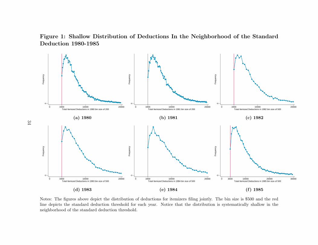
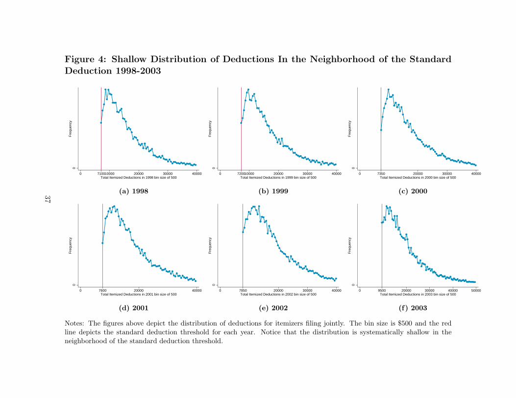
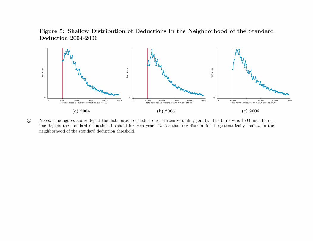
If taxpayers are claiming the standard deduction even though they could benefit from item-

izing, the density of deductions should be shallow in the neighborhood of the standard de-

6

duction. This shallowness is observed for any year non-reform year (figures 1, 2, 3, 4 and

5). To show the causal relationship between the standard deduction and the shallow density

in the neighborhood of the standard deduction, I use four reforms that increases the stan-

dard deduction amount by a large proportion in 1971, 1972, 1989 and 2003 (see table ??). I

observe that the shallowness follows precisely the standard deduction threshold (figure 7, 6

and 8). I develop a method to recover the counterfactual density of deductions by using the

year that precedes each reform. I use this counterfactual to estimate the cost of itemizing

by measuring the magnitude of the missing mass caused by the proximity to the standard

deduction.

3.1 The Density of Deductions Is Shallow In the Neighborhood of

the Standard Deduction

If some taxpayers are claiming the standard deduction even though their total itemized deduc-

tions are greater than the standard deduction amount the distribution of the total itemized

deductions should be shallow in the neighborhood of the standard deduction threshold.

In order to verify this assertion, I graph the density of deductions for all years ranging from

1980 to 2006 by bin sizes of $500. Notice that the closest bin to the standard deduction is

only composed of itemizers whose deductions are strictly larger than the standard deduction

amount. Figures 1, 2, 3, 4 and 5 show the distribution of itemized deductions for years ranging

from 1980 to 2006 and for joint filers (this effect is consistent across filing categories). We

can notice that the distribution is systematically shallow in the neighborhood of the standard

deduction matching my initial hypothesis.

There are no observations on the left of the standard deduction threshold because non-

itemizers are not required to report their deductions.

Is the true density of deductions discontinuous at the standard deduction? It is likely, but

without observing the density on the left-hand side of the standard deduction threshold, I

cannot rule-out a smooth density. Approximately two-thirds of taxpayers claim the standard

deduction which means that the density below the standard deduction threshold cannot be

increasing from zero onwards and then connects with the density on the right-hand side of the

standard deduction, as this would fail to account for a large portion of the population. If the

density is smoothly decreasing on the left-hand side of the standard deduction threshold and

7

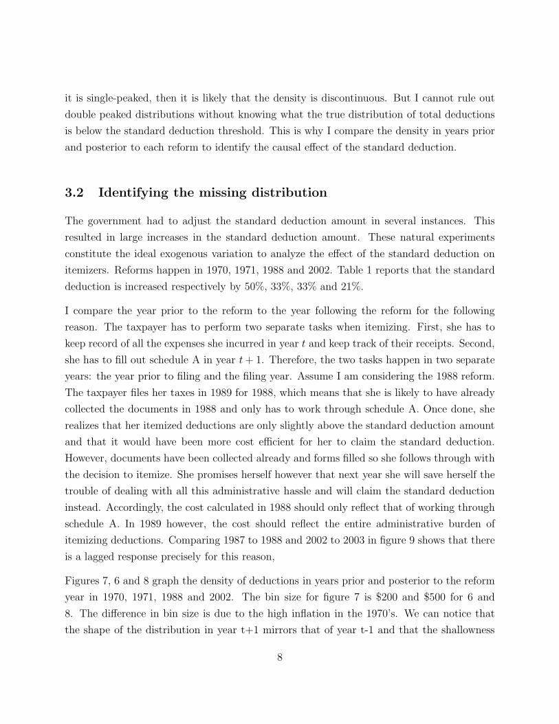
it is single-peaked, then it is likely that the density is discontinuous. But I cannot rule out

double peaked distributions without knowing what the true distribution of total deductions

is below the standard deduction threshold. This is why I compare the density in years prior

and posterior to each reform to identify the causal effect of the standard deduction.

3.2 Identifying the missing distribution

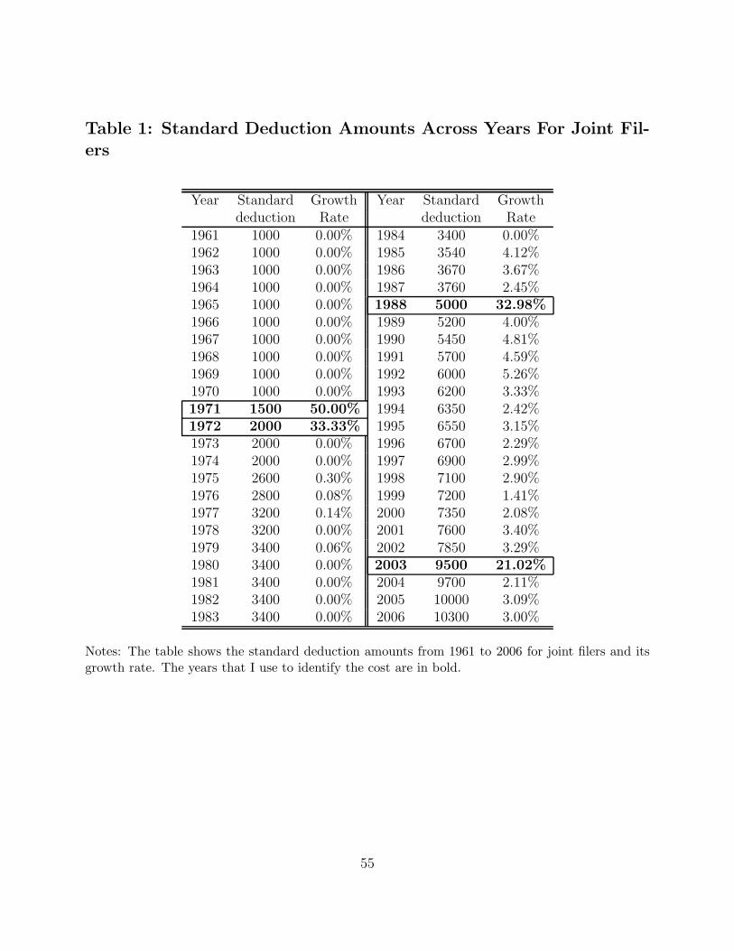
The government had to adjust the standard deduction amount in several instances. This

resulted in large increases in the standard deduction amount. These natural experiments

constitute the ideal exogenous variation to analyze the effect of the standard deduction on

itemizers. Reforms happen in 1970, 1971, 1988 and 2002. Table 1 reports that the standard

deduction is increased respectively by 50%, 33%, 33% and 21%.

I compare the year prior to the reform to the year following the reform for the following

reason. The taxpayer has to perform two separate tasks when itemizing. First, she has to

keep record of all the expenses she incurred in year t and keep track of their receipts. Second,

she has to fill out schedule A in year t+ 1. Therefore, the two tasks happen in two separate

years: the year prior to filing and the filing year. Assume I am considering the 1988 reform.

The taxpayer files her taxes in 1989 for 1988, which means that she is likely to have already

collected the documents in 1988 and only has to work through schedule A. Once done, she

realizes that her itemized deductions are only slightly above the standard deduction amount

and that it would have been more cost efficient for her to claim the standard deduction.

However, documents have been collected already and forms filled so she follows through with

the decision to itemize. She promises herself however that next year she will save herself the

trouble of dealing with all this administrative hassle and will claim the standard deduction

instead. Accordingly, the cost calculated in 1988 should only reflect that of working through

schedule A. In 1989 however, the cost should reflect the entire administrative burden of

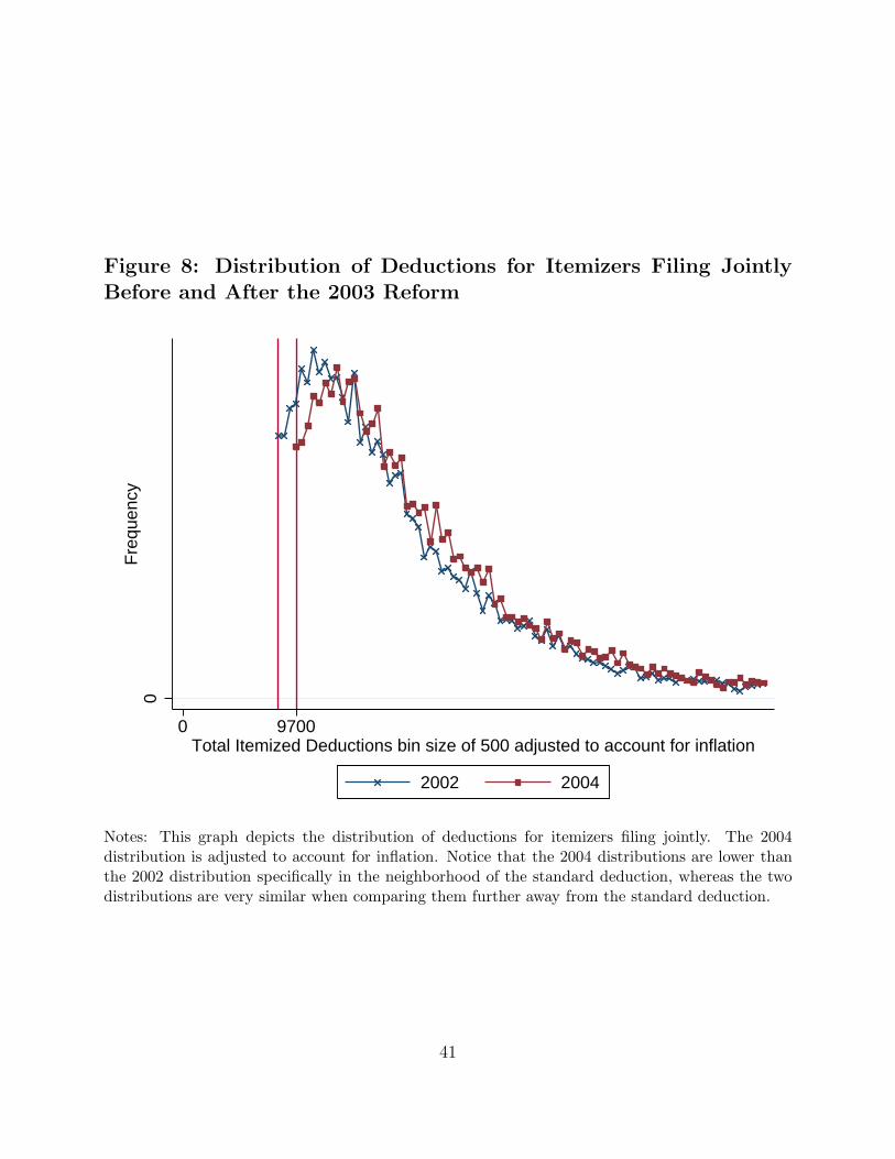
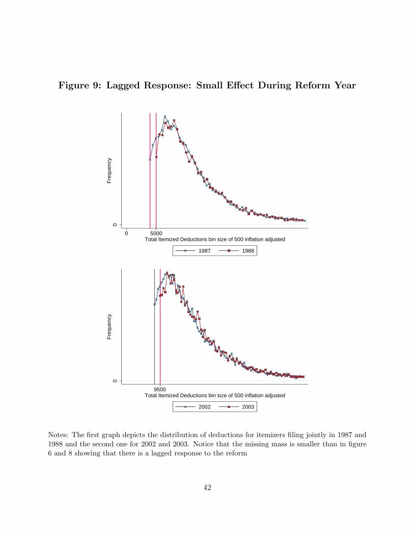
itemizing deductions. Comparing 1987 to 1988 and 2002 to 2003 in figure 9 shows that there

is a lagged response precisely for this reason,

Figures 7, 6 and 8 graph the density of deductions in years prior and posterior to the reform

year in 1970, 1971, 1988 and 2002. The bin size for figure 7 is $200 and $500 for 6 and

8. The difference in bin size is due to the high inflation in the 1970’s. We can notice that

the shape of the distribution in year t+1 mirrors that of year t-1 and that the shallowness

8

very precisely follows the new standard deduction threshold. This shows that taxpayers are

claiming the standard deduction once it is increased even though their deductions are larger

than the standard deduction. Notice that the missing mass is smaller in the 1970’s compared

to later years. Inflation was extremely large in the 1970’s suggesting that eventhough the

nominal cost could be small, the real one is likely to be of the same magnitude.

3.3 Adjusting the distribution from year to year

Given that I am comparing two separate years, I need to adjust for the effect of inflation.

Adjusting the previous year’s density by multiplying by inflation is imperfect as the deduc-

tions are not guaranteed to vary with inflation. In fact most of the deductions are likely to

remain fixed in nominal terms. In case of charitable contributions it is unlikely that individ-

uals would adjust from year to year the amount of contributions they make by the inflation

amount). In the case of the mortgage deduction, interest rates can be fixed, indexed to

inflation or indexed to other variables.

In addition, even if the difference is small between the inflation adjustment and the actual

adjustment it can create a significant distortion when comparing across two years. Assume

that inflation is constant across years and equal to π and that the inflation adjustment over

corrects the distribution by ǫ. This means that when comparing year t’s distribution to year

t+1, year t will be over adjusted by ǫ. But when comparing year t to year t+2 (my main

identification), year t is adjusted by (1 + π + ǫ)(1 + π + ǫ) = (1 + ǫ)2 + ǫ(2 + ǫ+ 2π). When

comparing distributions that are two years apart, the corrected distribution is over corrected

by ǫ(2 + ǫ+ 2π).

Tax data probably constitutes the best source to calculate this growth rate. I calculate

the weighted average of deductions in year t-1 and compare it to that of year t+1. The

ratio gives me the growth rate of deductions. In years when there is a reform, I restrict the

sample so that it is far enough from the neighborhood of the new standard deduction to avoid

having the effect of the reform contaminate the natural growth of the deduction. Consider

the 1988 reform. It increased the standard deduction from $3,760 to $5,000. If I were

to consider all taxpayers with deductions above $5,000, the growth rate would be biased

upwards, since many taxpayers stop itemizing and start claiming the standard deduction

when their itemized deductions are close to $5,000 resulting in a higher proportion of high

9

itemizers (since taxpayers who claim the standard deduction are not accounted for). For

this reason, in years when there is a reform, I restrict the sample that I use to calculate the

growth rate to any itemizer who is 10 bins away from the standard deduction to ensure that

they are unlikely to switch to the standard deduction because they are close to it.

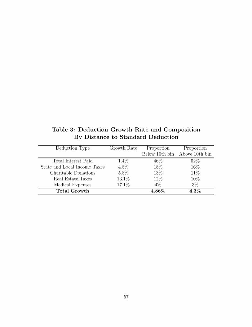
Next, I need to account for the fact that the compositions of deductions might be different

for those that have more deductions than others. This is a reasonable concern given that

deductions are correlated with incomes and high incomes tend to have a lower proportion

of charitable donations in their total deductions and more mortgage payments overall. Fur-

thermore, the growth rate is also likely to be deduction specific: charitable donations are less

likely than state taxes to grow at a rate that is close to inflation. To address this concern, I

calculate the proportion of each type of deductions for individuals that are more than 10 bins

away from the standard deduction and individuals that are less than 10 bins away from it. I

find that the proportions are indeed different, although the difference is small. I then calcu-

late the growth rate of each deduction and use it along with the proportion of deductions to

find the growth rate for individuals below the threshold. I find that the two growth rates are

fairly similar. The results are reported in table 4. The first column shows the growth rate

of each category of deductions. The second one calculates the proportion of deductions for

each group of taxpayers: those that are less than 10 bins away from the standard deduction

and those that are more than 10 bins away from the standard deduction. The remaining

categories of deductions, such as moving expenses or casualty or theft loss are not included

because they represent less than 1% of the proportion of deductions.

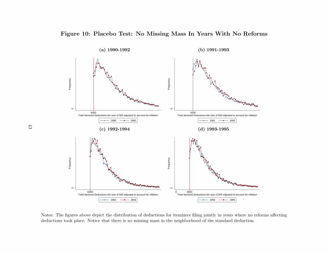
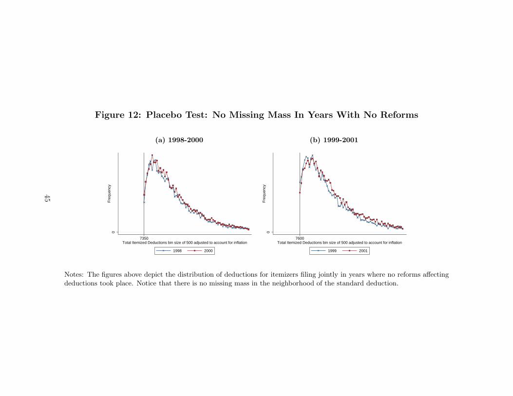
To verify that this adjustment is reasonable, I carry placebo tests on years when there was

no reform and using the same adjustment I verify that the distributions from two separate

years are indeed overlapping in figures 10 and 11. I exclude years prior to 1990 because the

standard deduction was not indexed to inflation prior to 1986 and from 1987 to 1989 reforms

affected the distribution (including the standard deduction reform).

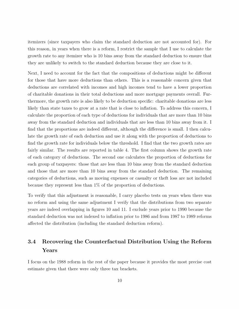
3.4 Recovering the Counterfactual Distribution Using the Reform

Years

I focus on the 1988 reform in the rest of the paper because it provides the most precise cost

estimate given that there were only three tax brackets.

10

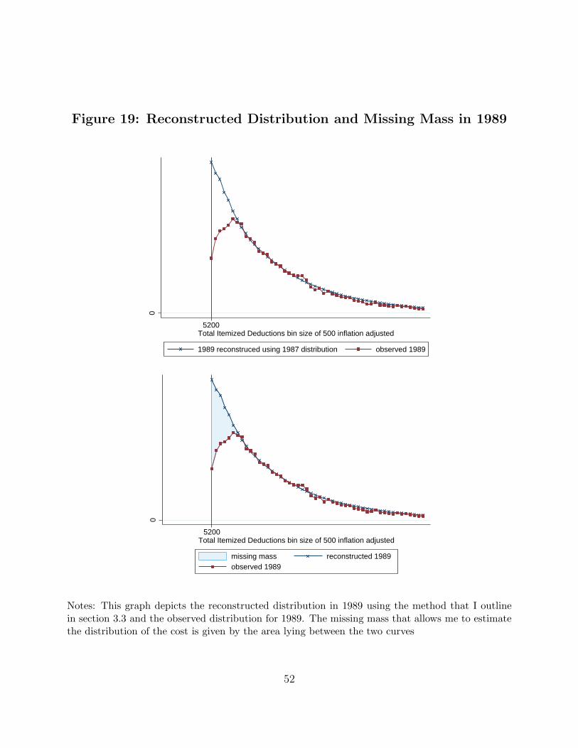
To calculate the cost of itemizing deductions, I use the following approach. I first create bins

of a given size. For the 1989 reform, I use a bin size of $500. I then calculate the weighted

frequency of individuals located in those bins. I subtract the size of the 1989 bin from the

size of the corresponding bin in 1987 after adjusting the amounts to account for inflation (see

previous section).

This approach allows me to measure the percentage of individuals that claim the standard

deduction even though their total itemized deductions exceed the standard deduction amount

by multiples of $500.

Once I get those percentages, I need to adjust the 1987 distribution as it might be distorted

by its proximity to the standard deduction amount. For clarity I associate each bin with a

number that denotes its distance from the standard deduction amount. For example, in 1987

the standard deduction amount is $3750. This means that bin [3750, 4250] will be called bin

number 1 in 1987 and bin [4750, 5250] will be called bin number 3 in 1987. Bins in 1989

are defined in a similar way relative to the standard deduction amount of $5,200: bin [5200,

5700] is bin number 1 and bin [6200, 6700] is bin number number 3.

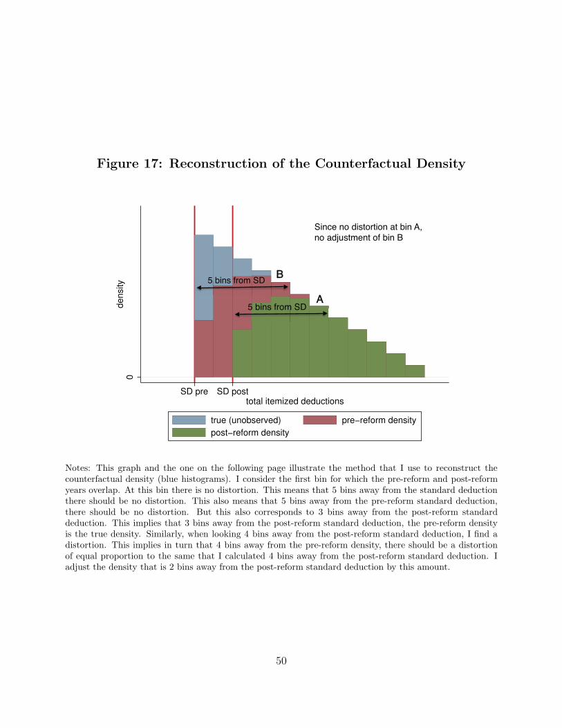
To perform the adjustment, I consider the last bin in 1989 for which the 1987 and 1989

curves are not overlapping. Figure 6 shows that these are bin number 6 in 1989 and bin 8 in

1987. The difference between 1987 and 1989 for this bin would give me the true distribution

provided that bin number 8 in 1987 is not distorted. To check for whether bin number 6

in 1987 gives me the true density or not I turn to the 1989 distribution and I look at the

distortion for bin number 8 in 1989 and compare it to bin number 10 in 1987. I find that the

two curves are overlapping in bin number 8 in 1989. This means that the standard deduction

is unlikely to distort the behavior of a taxpayer who is located 6 bins away from the standard

deduction. I can therefore safely infer that the difference between 1987 and 1989 corresponds

to the true distortion for this bin. I repeat this process for every single bin until I reach the

very first bin. Starting with bin number 4 in 1987, the 1987 distribution does not provide

me with the true counterfactual anymore. I previously calculated the true distortion that

occurs at bin number 4 by comparing the 1987 and 1989 distribution at bin number 4 in

1989. Denote that distortion by d%. I can use this distortion to correct the 1987 distribution

and form the counterfactual by adding d% to the 1987 distribution in bin number 4. This

process allows me to reconstruct the counterfactual when the 1987 distribution is distorted.

11

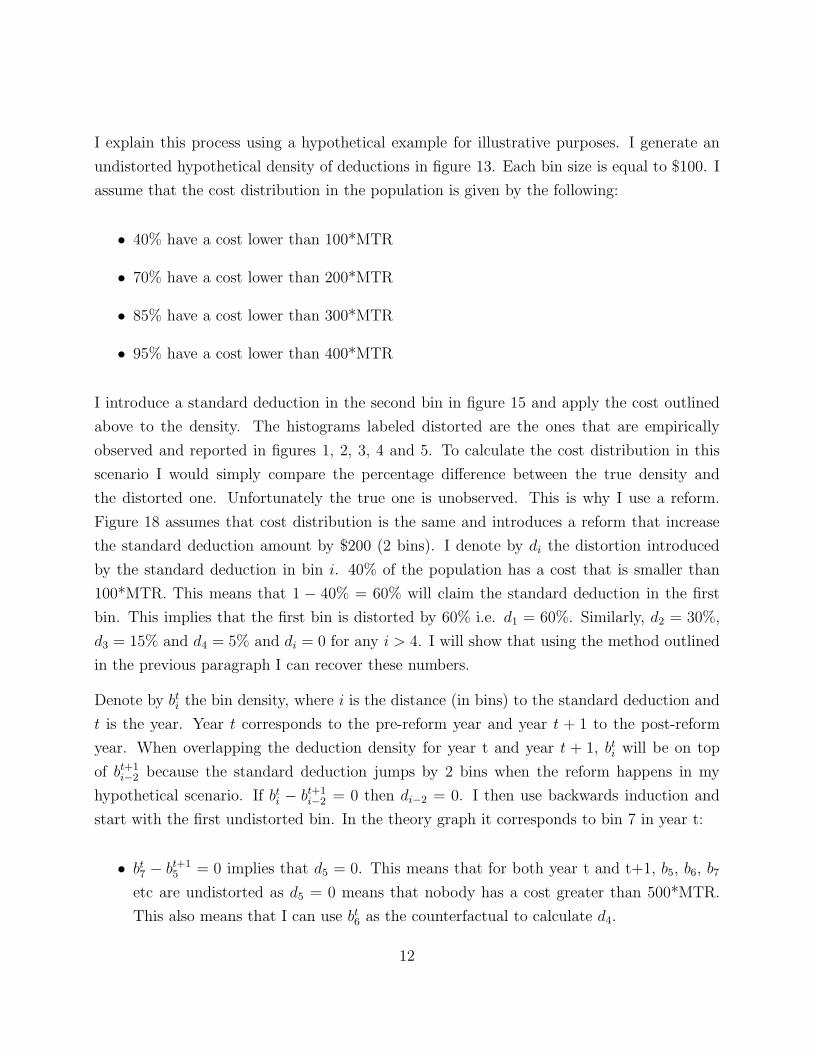
I explain this process using a hypothetical example for illustrative purposes. I generate an

undistorted hypothetical density of deductions in figure 13. Each bin size is equal to $100. I

assume that the cost distribution in the population is given by the following:

• 40% have a cost lower than 100*MTR




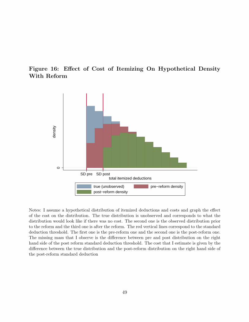
I introduce a standard deduction in the second bin in figure 15 and apply the cost outlined

above to the density. The histograms labeled distorted are the ones that are empirically

observed and reported in figures 1, 2, 3, 4 and 5. To calculate the cost distribution in this

scenario I would simply compare the percentage difference between the true density and

the distorted one. Unfortunately the true one is unobserved. This is why I use a reform.

Figure 18 assumes that cost distribution is the same and introduces a reform that increase

the standard deduction amount by $200 (2 bins). I denote by di the distortion introduced

by the standard deduction in bin i. 40% of the population has a cost that is smaller than

100*MTR. This means that 1 − 40% = 60% will claim the standard deduction in the first

bin. This implies that the first bin is distorted by 60% i.e. d1 = 60%. Similarly, d2 = 30%,

d3 = 15% and d4 = 5% and di = 0 for any i > 4. I will show that using the method outlined

in the previous paragraph I can recover these numbers.

Denote by bti the bin density, where i is the distance (in bins) to the standard deduction and

t is the year. Year t corresponds to the pre-reform year and year t + 1 to the post-reform

year. When overlapping the deduction density for year t and year t + 1, bti will be on top

of bt+1

i−2 because the standard deduction jumps by 2 bins when the reform happens in my

hypothetical scenario. If bti − bt+1

i−2= 0 then di−2 = 0. I then use backwards induction and

start with the first undistorted bin. In the theory graph it corresponds to bin 7 in year t:

• bt7 − bt+1

5 = 0 implies that d5 = 0. This means that for both year t and t+1, b5, b6, b7

etc are undistorted as d5 = 0 means that nobody has a cost greater than 500*MTR.

This also means that I can use bt6 as the counterfactual to calculate d4.

12

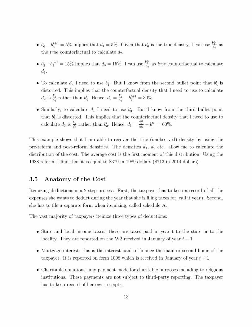
• bt6 − bt+1

4 = 5% implies that d4 = 5%. Given that bt6 is the true density, I can useb874

d4as

the true counterfactual to calculate d2.

• bt5− bt+1

3 = 15% implies that d3 = 15%. I can useb873

d3as true counterfactual to calculate

d1.

• To calculate d2 I need to use bt4. But I know from the second bullet point that bt4 is

distorted. This implies that the counterfactual density that I need to use to calculate

d2 isbt4

d4rather than bt4. Hence, d2 =

bt4

d4− bt+1

2 = 30%.

• Similarly, to calculate d1 I need to use bt3. But I know from the third bullet point

that bt3 is distorted. This implies that the counterfactual density that I need to use to

calculate d3 isbt3

d3rather than bt3. Hence, d1 =

b873

d3− b891 = 60%.

This example shows that I am able to recover the true (unobserved) density by using the

pre-reform and post-reform densities. The densities d1, d2 etc. allow me to calculate the

distribution of the cost. The average cost is the first moment of this distribution. Using the

1988 reform, I find that it is equal to $379 in 1989 dollars ($713 in 2014 dollars).

3.5 Anatomy of the Cost

Itemizing deductions is a 2-step process. First, the taxpayer has to keep a record of all the

expenses she wants to deduct during the year that she is filing taxes for, call it year t. Second,

she has to file a separate form when itemizing, called schedule A.

The vast majority of taxpayers itemize three types of deductions:

• State and local income taxes: these are taxes paid in year t to the state or to the

locality. They are reported on the W2 received in January of year t + 1

• Mortgage interest: this is the interest paid to finance the main or second home of the

taxpayer. It is reported on form 1098 which is received in January of year t + 1

• Charitable donations: any payment made for charitable purposes including to religious

institutions. These payments are not subject to third-party reporting. The taxpayer

has to keep record of her own receipts.

13

In addition, some taxpayers also claim other taxes (real estate or sales taxes in some years),

other interest expenses (credit-card interest in some years), casualty or theft losses, medical

and dental expenses and miscellaneous deductions.

Schedule A is relatively easy to fill out especially if the taxpayer only needs to itemize the

most common deductions outlined above. All she has to do is copy numbers from the 1098,

W2 or charitable contribution receipts, sum them up and copy the sum in the 1040 form.

There are no complicated tax schedules nor intricate tax operations. Record keeping is more

time consuming as one has to archive the various evidence of expenses to be able to recover

them when the tax season arrives. It is however easier to keep track of deductions that are

third-party reported given that taxpayers receive the W2 and 1098 in January of year t+ 1.

3.6 Cost Estimates

3.6.1 The 1988 reform

The 1988 reform provides the most precise cost estimate: there were no reforms affecting

deductions in 1988 or 1989 and the only reforms affecting the 1987 distribution do not have

a lagged effects (discussed later). I estimate the costs using the 1971-1972 and 2003 reforms

but 1988 reform cost estimates are the most accurate ones.

My estimates show that taxpayers are willing to forego $378 in 1989. The average wage

for the taxpayers whom I identify as foregoing tax benefits varies between $8 for the lowest

income group to $14 for the highest income one. A back of the envelope calculation implies

that taxpayers perceive that itemizing requires more than 20 hours.

Every year, the IRS provides cost estimates for each tax form including both the time required

to fill out the form and to keep track of the receipts. In 1989, the IRS estimates that the

average taxpayer needs 1 hour and 1 minute to fill out schedule A, 2 hours and 47 minutes for

record keeping, 26 minutes to learn about the form and 20 minutes to copy and assemble the

documents before sending them to the IRS. This totals 4 hours and 34 minutes. Guyton et al.

(2003) describe the methods used by the IRS to calculate the cost. They explain that the

IRS uses the Individual Taxpayer Burden Model developed jointly with IBM to calculate the

cost of filing taxes. The IRS inputs estimates from surveys in the model that provides the

cost estimates. However, the specifics of the model are unclear.

14

3.6.2 The 2003 reform

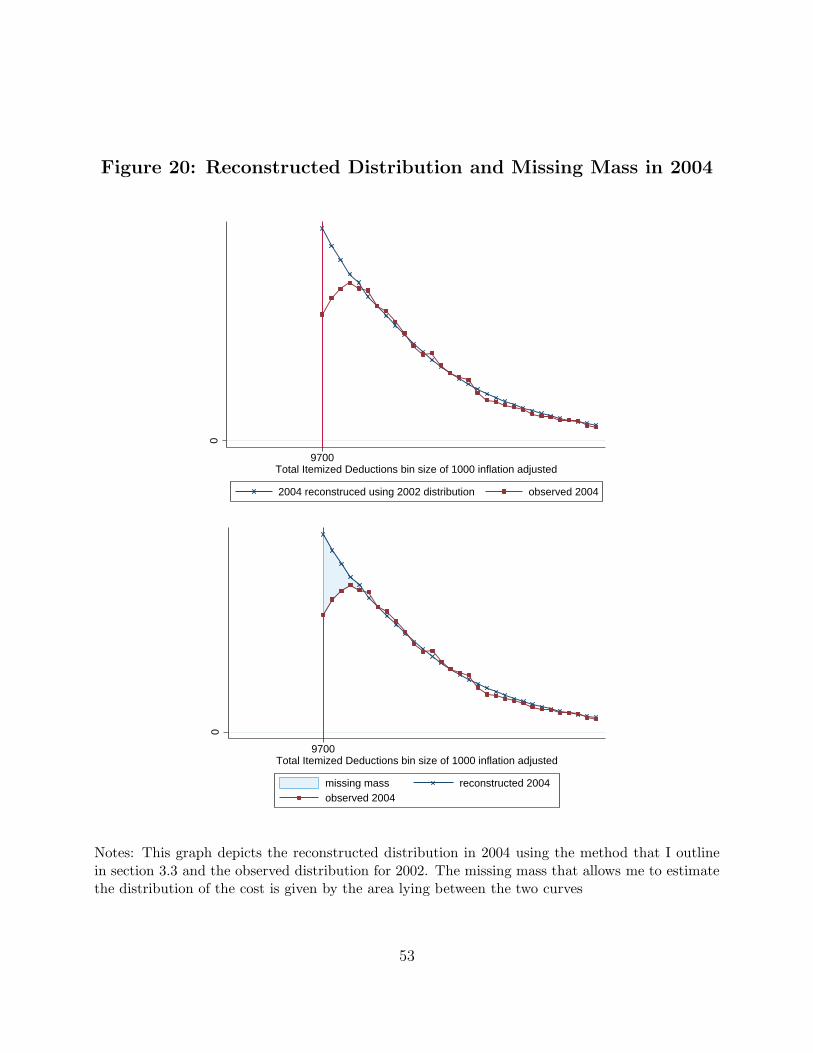
In 2003, the standard deduction is increased from $7,850 to $9,500. Similarly to 1988,

comparing the density of itemizers in 2002 to 2004 in figure 8 we can see that individuals

who are close to the standard deduction after the reform stop itemizing.

To estimate the cost of itemizing, I use a similar approach to the one outlined above. There

are however some caveats to using the 2003 reform:

• In 2003, the government allowed taxpayers to deduct the highest of state and local

income taxes and state sales taxes. This is likely to bias the cost estimates downwards

as deductions are likely to increase overall.

• The proportion of electronic filers increases significantly from 2002 to 2004 possibly

because of the technological expansion of the early 2000’s. If e-filing reduces the cost of

complying with taxes then it is also likely to bias the cost estimates downwards. This

is both a limitation and an opportunity: I will use later to estimate the effect of e-filing

on the cost of compliance.

• There is heterogeneity in the marginal tax rate for individuals close to the standard

deduction threshold. Taxpayers who are close to the standard deduction threshold

have a marginal tax rate of 10%, 15%, 25% and 28%. Whereas in 1988 I could use one

marginal tax rate, here I have to take an average of the marginal tax rates to calculate

the foregone benefits.

The cost estimated is equal to $191. There is a strong relationship between income and

foregone benefits. This means that to compare it to the 1988 cost estimate, I need to adjust

for the fact that individuals who are close to the standard deduction in 2003 are relatively

poorer.

4 What Are the Main Drivers of the Cost?

Taxpayers are willing to forego large tax benefits to avoid having to itemize. This behavior

reveals that the cost of itemizing is fairly large. What drives such a high cost? Itemizing

involves two tasks: record keeping and filling out schedule A. In this section, I show that

15

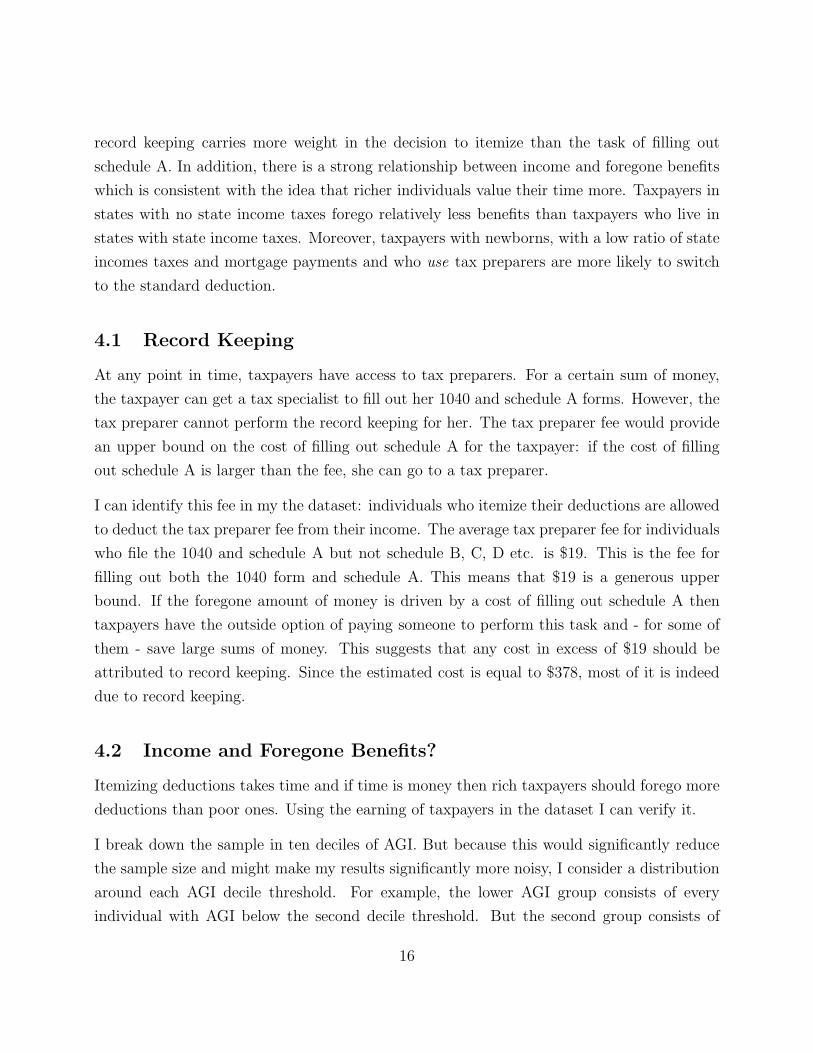
record keeping carries more weight in the decision to itemize than the task of filling out

schedule A. In addition, there is a strong relationship between income and foregone benefits

which is consistent with the idea that richer individuals value their time more. Taxpayers in

states with no state income taxes forego relatively less benefits than taxpayers who live in

states with state income taxes. Moreover, taxpayers with newborns, with a low ratio of state

incomes taxes and mortgage payments and who use tax preparers are more likely to switch

to the standard deduction.

4.1 Record Keeping

At any point in time, taxpayers have access to tax preparers. For a certain sum of money,

the taxpayer can get a tax specialist to fill out her 1040 and schedule A forms. However, the

tax preparer cannot perform the record keeping for her. The tax preparer fee would provide

an upper bound on the cost of filling out schedule A for the taxpayer: if the cost of filling

out schedule A is larger than the fee, she can go to a tax preparer.

I can identify this fee in my the dataset: individuals who itemize their deductions are allowed

to deduct the tax preparer fee from their income. The average tax preparer fee for individuals

who file the 1040 and schedule A but not schedule B, C, D etc. is $19. This is the fee for

filling out both the 1040 form and schedule A. This means that $19 is a generous upper

bound. If the foregone amount of money is driven by a cost of filling out schedule A then

taxpayers have the outside option of paying someone to perform this task and - for some of

them - save large sums of money. This suggests that any cost in excess of $19 should be

attributed to record keeping. Since the estimated cost is equal to $378, most of it is indeed

due to record keeping.

4.2 Income and Foregone Benefits?

Itemizing deductions takes time and if time is money then rich taxpayers should forego more

deductions than poor ones. Using the earning of taxpayers in the dataset I can verify it.

I break down the sample in ten deciles of AGI. But because this would significantly reduce

the sample size and might make my results significantly more noisy, I consider a distribution

around each AGI decile threshold. For example, the lower AGI group consists of every

individual with AGI below the second decile threshold. But the second group consists of

16

an AGI that is comprised between the first and the third AGI decile etc. Notice that some

individuals will simultaneously belong to two groups: for example individuals whose AGI falls

in the second AGI decile will belong both the the first group (AGI below the second AGI

threshold) and the second group (AGI greater than the first decile threshold but smaller than

the third decile threshold). This overlap is not a concern because the goal of this breakdown

is to graph the relationship between AGI and foregone benefits. The precise location of a

point in the AGI/foregone benefit space is of no particular importance. It only matters in

depicting the general trend of the relationship.

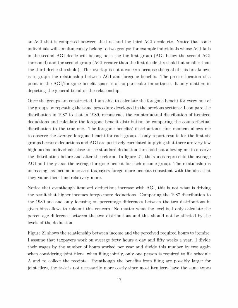
Once the groups are constructed, I am able to calculate the foregone benefit for every one of

the groups by repeating the same procedure developed in the previous sections: I compare the

distribution in 1987 to that in 1989, reconstruct the counterfactual distribution of itemized

deductions and calculate the foregone benefit distribution by comparing the counterfactual

distribution to the true one. The foregone benefits’ distribution’s first moment allows me

to observe the average foregone benefit for each group. I only report results for the first six

groups because deductions and AGI are positively correlated implying that there are very few

high income individuals close to the standard deduction threshold not allowing me to observe

the distribution before and after the reform. In figure 21, the x-axis represents the average

AGI and the y-axis the average foregone benefit for each income group. The relationship is

increasing: as income increases taxpayers forego more benefits consistent with the idea that

they value their time relatively more.

Notice that eventhough itemized deductions increase with AGI, this is not what is driving

the result that higher incomes forego more deductions. Comparing the 1987 distribution to

the 1989 one and only focusing on percentage differences between the two distributions in

given bins allows to rule-out this concern. No matter what the level is, I only calculate the

percentage difference between the two distributions and this should not be affected by the

levels of the deduction.

Figure 21 shows the relationship between income and the perceived required hours to itemize.

I assume that taxpayers work on average forty hours a day and fifty weeks a year. I divide

their wages by the number of hours worked per year and divide this number by two again

when considering joint filers: when filing jointly, only one person is required to file schedule

A and to collect the receipts. Eventhough the benefits from filing are possibly larger for

joint filers, the task is not necessarily more costly since most itemizers have the same types

17

of deductions, only higher amounts. Using a revealed preference argument, this gives me a

relationship between the AGI groups and the revealed time that each group thinks itemizing

requires.

Although of a lower magnitude and significance I find an increasing relationship between

the value of time of a given taxpayer and the AGI deciles. The estimates range between 20

hours for the lowest income group to 30 hours for the highest one. If the relationship had

been constant, it would have meant that richer and poorer taxpayers perceive the decision

to itemize to be equally time consuming, but here the relationship is increasing. This could

be interpreted in several ways:

• It could be that richer individuals truly spend more time itemizing because they have

more deductions. It is true that rich individuals have higher amounts of deductions

but it is unlikely that they require more time to itemize them. The cost of itemizing

is mostly fixed and does not generally increase in the amount of the deduction. If one

taxpayer has $10,000 worth of mortgage interest, she will most likely spend the same

amount of time itemizing them as a taxpayer who has $100,000 since they have to spend

the same amount of time archiving the forms and entering the numbers on schedule A.

• It is likely that what this relationship reveals is that individuals have different pref-

erences over filing their taxes relative to working an extra hour at their regular jobs.

What I am calculating is the marginal rate of substitution (MRS) between an hour of

work and an hour of filing taxes. The MRS could be different for two different individ-

uals for two reasons: they enjoy working at their regular job equally but dislike filing

taxes differently or they enjoy working at their jobs differently but dislike filing taxes

equally. The most plausible story is that better paying jobs are usually more fulfilling

and that individuals equally dislike filing taxes, which explains that the revealed value

of time for rich households is higher than for poor households.

4.3 Who Is More Likely to Switch to the Standard Deduction?

4.3.1 Identification Strategy

I use the panel dataset to identify the reasons that make a taxpayer more likely to switch to

the standard deduction. I focus on taxpayers who itemize deductions in year t and observe

18

their decisions in year t+1 by creating a dummy variable that equals 1 if the taxpayer switches

to the standard deduction in year t + 1. I also make sure to drop individuals who have to

file other schedules (B, C etc) as they could bias the results. I do not consider individuals

who switch from claiming the standard deduction to itemizing because this decision is not

as easily available as the opposite one. A person with deductions in excess of the standard

deduction threshold can easily decide between itemizing or not. But a person that is claiming

the standard deduction is likely to have too few deductions in total to be able to itemize. All

my results are clustered at the individual level. Clustering at the state level yields similar

results.

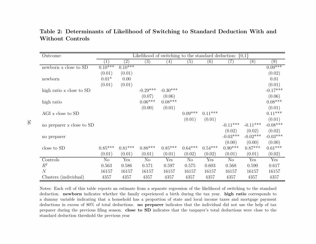
I regress the variable that indicates that the individual is switching to the standard deduction

on several variables of interest that I explain below. I also control for the level of deductions

in year t, a polynomial of AGI, marital status, year fixed effects and states. The results are

reported in table 2.

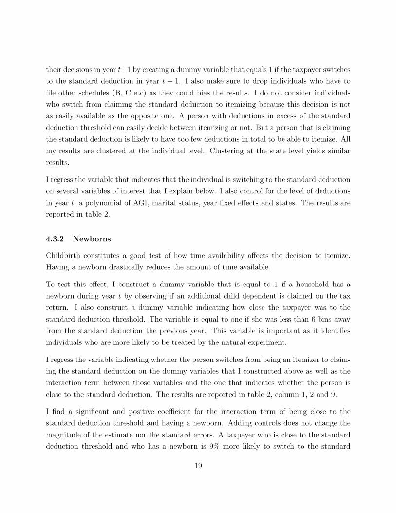
4.3.2 Newborns

Childbirth constitutes a good test of how time availability affects the decision to itemize.

Having a newborn drastically reduces the amount of time available.

To test this effect, I construct a dummy variable that is equal to 1 if a household has a

newborn during year t by observing if an additional child dependent is claimed on the tax

return. I also construct a dummy variable indicating how close the taxpayer was to the

standard deduction threshold. The variable is equal to one if she was less than 6 bins away

from the standard deduction the previous year. This variable is important as it identifies

individuals who are more likely to be treated by the natural experiment.

I regress the variable indicating whether the person switches from being an itemizer to claim-

ing the standard deduction on the dummy variables that I constructed above as well as the

interaction term between those variables and the one that indicates whether the person is

close to the standard deduction. The results are reported in table 2, column 1, 2 and 9.

I find a significant and positive coefficient for the interaction term of being close to the

standard deduction threshold and having a newborn. Adding controls does not change the

magnitude of the estimate nor the standard errors. A taxpayer who is close to the standard

deduction threshold and who has a newborn is 9% more likely to switch to the standard

19

deduction. Notice that this effect accounts for the fact that income and total deductions

tend to increase following birth.

If itemizing was not a time consuming task, this result would be rather counter-intuitive:

prior to having a child one should expect incomes to increase and since deductions tend to be

positively correlated with income, one should observe a higher probability of itemizing. Here

I observe the opposite. This means that ceteris paribus, child birth increases the chances

of switching to the standard deduction for itemizers precisely because newborns are time

consuming and require a lot of attention that might be drawn from other tasks that are not

as urgent.

This analysis shows that an exogenous shock such as child birth has significant effects over the

decision to itemize providing evidence of the fact that itemizing is time consuming indeed. A

complementary explanation is that child birth introduces organizational challenges in the life

of the taxpayer. A rational taxpayer should be able to foresee these challenges and schedule

her time so as to be able to itemize once taxes are due. A present-biased one might not be

able to do so if she is naive about her procrastination. I will return to this distinction in a

later section and explain its importance from a policy perspective.

4.3.3 High Ratio of Third Party Reported Deductions

The mortgage payment deduction and the state and local income tax deduction are different

from the other deductions. They are third-party reported implying that taxpayers receive

a “statement” in the form of a 1098 or W2 in January of year t + 1, significantly reducing

the record keeping cost. It is also harder to adjust them in the short run to respond to tax

incentives.

I construct a dummy variable equal to 1 if more than 80% of the deductions of a given

taxpayer are composed of state and local income taxes and mortgage payments. I follow the

same procedure as previously outlined. The results are reported in table 2 columns 3, 4 and

9. The regression shows that a taxpayer who has a high proportion of these two deductions

is 17% more likely to switch to the standard deduction when her deductions are close to the

standard deduction threshold. This can be interpreted in two ways:

• It could be that the overall cost is smaller because these two types of tax deductions

20

have a relatively lower record keeping cost because both the W2 and the 1098 are

received in January of year t + 1, closer to the tax filing season. The fact that the

record keeping cost is smaller if the receipts are sent closer to the tax filing season

suggests that forms are harder to find or more likely to get lost as time elapses possibly

because they are not properly archived.

• Alternatively it could be that these deductions are hard to adjust: a taxpayer cannot

reduce her mortgage payments or income as readily as she can reduce her charitable

donations. This suggests that the response of the treated taxpayers is real: when they

start claiming the standard deduction, they also reduce their charitable donations.

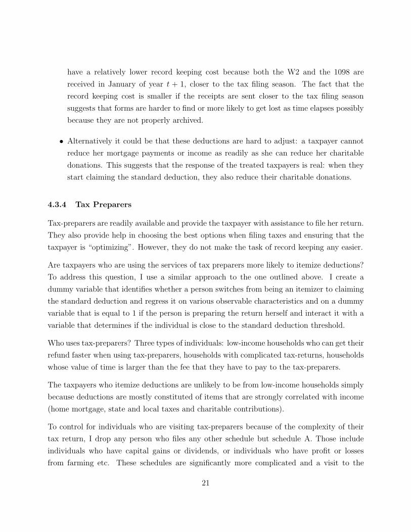
4.3.4 Tax Preparers

Tax-preparers are readily available and provide the taxpayer with assistance to file her return.

They also provide help in choosing the best options when filing taxes and ensuring that the

taxpayer is “optimizing”. However, they do not make the task of record keeping any easier.

Are taxpayers who are using the services of tax preparers more likely to itemize deductions?

To address this question, I use a similar approach to the one outlined above. I create a

dummy variable that identifies whether a person switches from being an itemizer to claiming

the standard deduction and regress it on various observable characteristics and on a dummy

variable that is equal to 1 if the person is preparing the return herself and interact it with a

variable that determines if the individual is close to the standard deduction threshold.

Who uses tax-preparers? Three types of individuals: low-income households who can get their

refund faster when using tax-preparers, households with complicated tax-returns, households

whose value of time is larger than the fee that they have to pay to the tax-preparers.

The taxpayers who itemize deductions are unlikely to be from low-income households simply

because deductions are mostly constituted of items that are strongly correlated with income

(home mortgage, state and local taxes and charitable contributions).

To control for individuals who are visiting tax-preparers because of the complexity of their

tax return, I drop any person who files any other schedule but schedule A. Those include

individuals who have capital gains or dividends, or individuals who have profit or losses

from farming etc. These schedules are significantly more complicated and a visit to the

21

tax-preparers might be necessary even for the most tax-savvy taxpayers.

I find that taxpayers who were using tax preparers in year t are 8% more likely to claim

the standard deduction in year t + 1. At first, this result can seem counterintuitive but it

is driven by the fact that taxpayers are not providing any help with record keeping and the

majority of the cost is due to record keeping. In addition, taxpayers who use tax preparers

are likely to be the ones who have a higher marginal disutility of filing taxes, so high that

they would rather have someone else do it. This is due to their aversion to taxes or to the

fact they are generally more busy. Therefore, it is not surprising that they would be more

likely to claim the standard deduction and is consistent with my previous findings.

4.4 States With No State Income Taxes

States with no income taxes represent an exogenous variation that can further our under-

standing of the decision to itemize. On the one hand, not having to file state taxes means that

the taxpayer is getting less benefits from itemizing since she cannot deduct those expenses

both on the federal return and on her state return. But on the other hand, not having to file

state taxes means that the taxpayer spends less time overall working on her taxes and can

potentially spend more time figuring out her tax deductions: her marginal disutility from

filing her taxes is lower if she does not have to file a state tax return in addition to the federal

return so she incurs less disutility from itemizing her deductions.

To answer this question, I break down states by whether they collect income taxes or not. In

1989, ten states had no income taxes: Alaska, Connecticut, Florida, Nevada, New Hampshire,

South Dakota, Tennessee, Texas, Washington and Wyoming. Individuals in these states

represent 13% of the entire sample. If I were to carry my main identification’s approach on

individuals that are not subject to state taxes and compare them to those that are subject

to state taxes, I could be biasing my results simply because the sample size of individuals

subject to state taxes is larger. With a larger sample size, the two curves of the distribution

of itemized deductions are likely to be less noisy and the curves will tend to intersect at a

further point. To address this issue, I break down the states that are subject to state taxes

in groups of similar sizes to that of the states with state taxes.

I find that individuals that reside in states with no state taxes have - on average - a lower

cost than individuals that live in states with state taxes. Individuals in states with no state

22

income taxes forego an average of $208 but states with state income taxes forego more than

twice this amount ($444).

This shows that the cost of filing taxes outweighs the benefits of having to deduct taxes on

one’s state taxes. Essentially, individuals who do not have to file a state return are less likely

to forego deductions probably because they spend less time filing their taxes overall since

they do not have to file state taxes and that gives them more time to work on their federal

return.

5 Making Sense of the Result

Most taxpayers have 4 to 5 receipts that need to be used to itemize. In addition, they have

to fill out schedule A. This is one of the easiest schedules as it only requires taxpayers to

enter numbers and sum them up and is unlikely to exceed an hour of work. I estimated that

a taxpayer perceives the task of itemizing as requiring more than 20 hours of work. This in

turn implies that each receipt requires an average of 4 hours of record keeping. This back of

the envelope calculation suggests that taxpayers are making a behavioral mistake when filing

their taxes. The following model offers a possible explanation of why the cost could be this

high. It builds upon O’Donoghue and Rabin (1999) and ODonoghue and Rabin (2008).

The model relies on the idea that the cost of record keeping continuously increases for every

day that the receipt is not archived as soon as it is received. Receipts that are not archived

can be lost or it could take more time to look for them. Knowing this, the rational taxpayer

archives her receipts as soon as she gets them. The naive taxpayer knows that it will be

more costly to archive the receipt the next day but because of her time inconsistency, she

procrastinates on it, leading to a large cost.

5.1 Setting

Assume for simplicity that the taxpayer only needs to itemize one deduction for example

for a charitable contribution she made. Then the taxpayer is facing two distinct costs when

considering the decision to itemize deductions. The first one is that of record keeping, denoted

here by c. The second one is filling out schedule A itself which is denoted by k.

Assume that the taxpayer has N periods to perform the two tasks, that they have to be

23

performed on two separate days and that record keeping has to be done before filling out

schedule A. This means that the last period in which record keeping can be performed is

N − 1 whereas filling out schedule A can be performed no later than in period N .

If the taxpayer succeeds in performing the two tasks she receives a one time benefit V . Once

the taxpayer gets the receipt for her charitable contribution, she can decide to archive it

immediately by incurring a cost c or archive it later and incur a larger cost c(1 + r) in the

next period.

I denote by δ the time-discount factor, β the present-bias parameter, t the period in which

the record keeping is performed and t+ u the period in which schedule A is filed.

In what follows, I use two definitions:

Definition 1: For given β, δ, c, k, (1 + r), t and u a task is said to be β-worthwhile if

−c(1 + r)t−1 + βδu(V − k) > 0.

Similarly:

Definition 2 For given δ, c, k, (1 + r), t and u a task is said to be δ-worthwhile if −c(1 +

r)t−1 + δu(V − k) > 0.

5.2 The Rational Taxpayer

The rational taxpayer has a standard utility function where per-period utility is discounted

by δ in the future. The total utility is given by

U = u0 +∑

i

δiui

The decision to itemize or claim the standard deduction can be written as follows:

maxt,u

δt(−c(1 + r)t−1 + δu(V − k))

Cost c is incurred as soon as taxpayers start the record keeping. If she waits an additional u

periods before filling out schedule A the cost of record keeping is multiplied by (1 + r).

24

Assuming that V − k > 0 i.e. that the benefit is large enough to justify filling out schedule

A, the taxpayer would want to perform this task as soon as possible, which means having

u = 1.

The taxpayer is left with choosing t such that:

maxt

δt(−c(1 + r)t−1 + δ(V − k))

Assume the taxpayer is contemplating the decision to perform the record keeping task in the

first period giving her: −c+ δ(V − k). She will only perform it if −c+ δ(V − k) > 0. And if

she waits an additional period she will receive δ(−c(1+ r)+ δ(V − k)), which is smaller than

the utility she would have enjoyed if the task had been performed in the first period. This

means that the rational taxpayer will either perform the tasks immediately or never perform

them. And she only performs the tasks if the project is worthwhile.

5.3 The Present-Biased Taxpayer

The present-biased taxpayer maximizes the following utility function:

u0 + β∑

i

δiui

Which in this context translates to:

maxt,u

δt(−c(1 + r)t−1 + βδu(V − k))

Since benefit V and cost k are both incurred in the same period, the taxpayer will not

procrastinate on performing the second task. This means that u = 1. The present-biased

taxpayer is maximizing:

maxt

δt(−c(1 + r)t−1 + βδ(V − k))

First, the task should be β-worthwhile i.e. it should be profitable for the present-biased

25

taxpayer to perform the task now. This happens when the following condition is satisfied:

−c + βδ(V − k) > 0

This condition simply states that the cost today should be smaller than the discounted net

benefit tomorrow.

Second, she can perform the record keeping now or she can wait and perform it next period.

She will prefer performing it next period if the following inequality is satisfied:

δt[−c(1 + r)t−1 + βδ(V − k)] < δt+1β[−c(1 + r)t−1 + δ(V − k)]

Which can be rewritten as:

For δ close to one, this inequality simplifies to:

β <1

1 + r

The taxpayer will procrastinate on archiving the charitable donation receipt if the (mis-)

perceived benefit of waiting an additional period is greater than the increase in archiving

cost.

Provided that it holds in period t = 0, the condition will hold in any subsequent period

t > 0 meaning that if the task is worthwhile but not performed in the very first period, the

taxpayer will procrastinate on it until the deadline.

Standard present-bias models show that with a strict deadline, naifs are likely to procrastinate

on completing a task but will perform it with certainty in the very last period. Filing taxes has

a strict deadline (April 15th) but I will show in what follows that - under certain conditions

- the naif will never perform the task simply because the expected benefit V has become too

low for the task to be β-worthwhile. The intuition is the following:

1. In the first stage, itemizing deductions is both β and δ-worthwhile. The present-biased

taxpayer would profit from performing the task now, but believes she would profit more

26

from doing it later and keeps on postponing the task to the next period.

2. In the second stage, the expected value of itemizing has decreased enough to make the

task not β-worthwhile anymore but is still δ-worthwhile. The taxpayer would not want

to perform the task now but still believes that she will do it tomorrow.

3. In the third stage, the task is neither β nor δ-worthwhile. The taxpayer does not want

to perform it neither now, nor later.

For this to happen, we need the task to stop being β-worthwhile and still be δ-worthwhile in

the next period. This is verified when the two following inequalities hold:

−c(1 + r)t−1 + β(V − k) < 0

−c(1 + r)t + V − k > 0

Which can be rewritten as follows:

β(V − k)

c

1

t−1

− 1 < r <(V − k)

c

1

t

− 1

Under this condition, the taxpayer keeps procrastinating on archiving the receipt until the

cost of doing it is too large to justify itemizing altogether. This result holds even for a

relatively small c and predicts that large benefits are foregone even if the initial cost would

not justify it for a rational taxpayer.

5.4 The Partially Naive Taxpayer

The partially naive taxpayer has self-control problems but is aware of them. She is able to

look forward, solve the problem backwards and realize that at some point, the task will stop

being β-worthwhile prompting her to perform the task before it is not worthwhile anymore.

Therefore her behavior is similar to that of the rational taxpayer.

27

5.5 Psychic Cost vs True Cost

My identification strategy shows that the cost of complying with taxes is very high and

certainly higher than that calculated by the IRS.

If taxpayers are truly not making any behavioral mistakes then the cost that I estimated is

the true cost of tax collection, suggesting that it is highly inefficient and needs reforming.

On the other hand, if the true model of the taxpayer’s behavior is one for which the taxpayer

makes a behavioral mistake by being time inconsistent, then one should be careful when

defining the cost of complying with taxes. The cost that I identified is composed of the true

cost of itemizing and a behavioral cost. This also means that the tax collection process is

not necessarily inefficient but rather that the behavior of the taxpayer drives the inefficiency.

If the government wants to reduce the cost of complying with taxes, it should not focus on

the process itself (having a standard deduction rather than itemized deductions) but should

focus on fixing the taxpayer’s biases.

6 Alternative Explanations

6.1 Role of Information and Cognitive Abilities

The increase in the standard deduction amounts makes it so that some taxpayers who were

itemizing deductions start claiming the standard deduction instead. This means that the

taxpayers that are foregoing tax benefits after the reform are well informed of the possibility

of itemizing deductions and have the cognitive abilities to do so.

6.2 Audit Probabilities

Could it be that taxpayers believe that itemizers are more likely to be audited than individuals

claiming the standard deduction? The probabilities of audit for this portion of the population

are lower than 1% and are virtually the same for individuals whose deductions are close to

the standard deduction and individuals who claim the standard deduction. Assume that an

audit would require one full day of work i.e. approximately $80 in my sample. This is smaller

than the foregone benefits implying that individuals would have an audit probability greater

than 1.

28

6.3 Other Reforms Affecting the Total Deduction Distribution?

Could there be any other exogenous variation affecting the distribution of itemized deductions

in 1989 and contaminating my main identification strategy? It is unlikely. One first check

for this is to look at the two distributions and specifically whether they are overlapping

on the portion that is away from the standard deduction. If they are not, then it means

that something else has happened besides the increase in the standard deduction threshold

affecting everybody not only those that are close to the threshold. Fortunately, the two

distributions are overlapping in regions away from the standard deduction suggesting that

the only effect that I am capturing is that of the standard deduction threshold being increased.

But for the sake of exhaustivity, I also look at all the reforms that could have affected the

distributions to rule them out as possible contaminants of my identification strategy.

The majority of the tax reforms happened following the TRA’86 and were enacted in 1987.

Among those, there were some deduction reforms. When comparing 1987 to 1989, I am

controlling for the TRA’86 reforms. But there might slow adjustment and lagged response

in 1988 or 1989. To rule this-out, I look at the deduction reforms following TRA’86 and find

that it is reasonable to assume that the adjustment is immediate. The deduction reforms

enacted in 1987 are the following (source: IRS):

• Increase of the threshold of medical deductions that are allowed from 5% in 1986 to 7.5%

of one’s AGI in 1987. There is no reason to assume that there will be a slow adjustment

in this case: the medical expense deduction amount should drop on aggregate in 1987

because less of it is allowed but one should not expect it to drop further than 1987.

• Sales taxes are not deductible anymore. For similar reasons, one should observe a

drop in the total deductions in 1987 as sales taxes were a large portion of it but there

should be no lagged effect: there could be a lagged effect for the aggregate purchases

of individuals in 1988 and 1989 but since sales taxes are not allowed as a deduction

anymore, this - by definition - should not affect the level of deductions anymore.

• The home mortgage interest deduction is subject to a new limit. The home mortgage

interest deductions for a given year are capped at the value of one’s house (plus reno-

vations). Anything in excess of the value of the house have to be deducted as personal

29

interest for which only 65% of the total value can be deducted. First, the IRS esti-

mated that very few taxpayers were affected by this reform since it is very rare that

one’s home mortgage interest in one given year exceeds the total value of one’s house.

Second, there is no reason to expect a drop in levels in the subsequent years. If a person

truly is affected by this reform, in 1987 she will be forced to claim less deduction than

she was previously claiming. Mortgages are indeed less flexible than regular sales and

assume that this person cannot adjust her mortgage payments for the next two years

and can only do so starting from 1989. What will happen in 1989? She will have an

incentive to reduce her mortgage payments to the level at which she deduct all of it i.e.

the level from 1987. Essentially, this would result in no real change in the levels after

1987 and can also be ruled-out as a possible contaminant of my identification strategy.

There are no other reforms affecting directly or indirectly the amount of itemized deductions

an individual can qualify for. Given the situation it is reasonable to assume that the only real

change to the level of itemized deductions from 1987 to 1989 is the increase in the standard

deduction threshold.

7 Policy Implications

7.1 Cost of Compliance

Policy makers had no precise estimates of the compliance cost. Most of the literature on the

compliance cost is based on survey evidence and its usual shortcomings (Slemrod and Sorum

(1985) and Blumenthal and Slemrod (1992)). To my knowledge, this is the first paper to

use a non-parametric approach along with administrative data to reveal the preferences of

taxpayers over the compliance cost. The costs are large, informing the policy maker that

the welfare lost because of compliance is of policy importance. The cost is also distortionary

as it impacts individuals differently: it varies with income, location in states with no state

taxes etc.

If the taxpayer is truly present biased, my model shows that the policy intervention should

not necessarily target the collection system but rather the behavior of the individual. In

light of my evidence, a policy that would target reducing the cost of filling out forms seems

misguided since the majority of the cost is precisely due to record keeping. One approach

30

could be to require less evidence of expenses when the taxpayer itemizes. This would prove

out to be efficient in reducing the compliance cost but is likely to result in more evasion.

The policy maker has to trade off the cost that evasion imposes on society and the cost that

compliance imposes on individuals.

My model also shows that there are relatively inexpensive policy interventions that can

significantly reduce the cost of compliance. Advocates of pre-populated forms argue that

they are likely to reduce evasion and mistakes by taxpayers. My results show that they are

also likely to improve the taxpayer welfare by reducing the compliance cost. Two of the three

most common deductions are state and local income taxes and mortgage interest payments.

Both of them are third-party reported implying that the IRS knows the amount of deductions

that the taxpayer qualifies for.

The use of electronic receipts is another channel through which record keeping costs can be

further reduced. Some employers issue the W2 online and some banks provide an electronic

1098. Keeping track of an electronic document can be much easier than a paper one. This

would only benefit taxpayers who have access to the Internet but it would not hurt the rest

and therefore constitutes a Pareto improvement

7.2 Screening Literature

There is a long tradition in public economics that emphasizes the benefits of conditioning

transfers on fixed characteristics and more particularly imposing transaction costs when

providing welfare to screen richer households from applying for them. To my knowledge there

was no empirical evidence confirming that transaction costs are larger for richer households.

This paper shows that it is the case and that such policy can be efficient. It warns however

that transaction costs need to be chosen with care as they can be relatively large and can

end up screening more income groups than optimal. They can also screen present-biased

taxpayers versus rational ones rather poor taxpayers versus poorer ones.

Similarly to Saez (2009) this paper also shows that details matter in designing a tax collection

system. Details that in theory should not have any impact over the decisions can result in

significant behavioral distortions.

31

8 Conclusion

How heavy is the burden of tax compliance? I answer this question by non-parametrically

calculating the cost of itemizing deductions. I show that it is in excess of $700 per taxpayer.

Rich taxpayers have a larger cost, consistent with the fact that they have a higher hourly

wage. Households with newborns are also more likely to switch to the standard deduction

because they have less time available. The magnitude of the cost has important policy

implications.

References

Bhargava, S. and D. Manoli (2011): “Why are benefits left on the table? assessing the

role of information, complexity, and stigma on take-up with an irs field experiment,” Tech.

rep., Working Paper.

Blumenthal, M. and J. Slemrod (1992): “The compliance cost of the US individual

income tax system: A second look after tax reform,” National Tax Journal, 185202.

Feenberg, D. R. and J. S. Skinner (1989): Sources of IRA saving, National Bureau of

Economic Research Cambridge, Mass., USA.

Guyton, J. L., J. F. O’Hare, M. P. Stavrianos, and E. J. Toder (2003): “Es-

timating the compliance cost of the US individual income tax,” National Tax Journal,

673688.

Jones, D. (2010): “Inertia and overwithholding: explaining the prevalence of income tax

refunds,” Tech. rep., National Bureau of Economic Research.

O’Donoghue, T. and M. Rabin (1999): “Doing it now or later,” American Economic

Review, 103124.

ODonoghue, T. and M. Rabin (2008): “Procrastination on long-term projects,” Journal

of Economic Behavior & Organization, 66, 161175.

Pitt, M. M. and J. Slemrod (1991): The compliance cost of itemizing deductions: Ev-

idence from individual tax returns, National Bureau of Economic Research Cambridge,

Mass., USA.

32

Rees-Jones, A. (2013): “Loss Aversion Motivates Tax Sheltering: Evidence From US Tax

Returns,” Available at SSRN.

Saez, E. (2009): “Details matter: The impact of presentation and information on the take-

up of financial incentives for retirement saving,” American Economic Journal: Economic

Policy, 1, 204228.

Slemrod, J. and N. Sorum (1985): The compliance cost of the US individual income tax

system, National Bureau of Economic Research Cambridge, Mass., USA.

33

Figure 1: Shallow Distribution of Deductions In the Neighborhood of the Standard

Deduction 1980-19850

Fre

quen

cy

0 3400 10000 20000Total Itemized Deductions in 1980 bin size of 200

(a) 1980

0F

requ

ency


(b) 1981

0F

requ

ency


(c) 1982

0F

requ

ency


(d) 1983

0F

requ

ency


(e) 1984

0F

requ

ency

0 3540 10000 20000 30000Total Itemized Deductions in 1985 bin size of 500

(f) 1985

Notes: The figures above depict the distribution of deductions for itemizers filing jointly. The bin size is $500 and the redline depicts the standard deduction threshold for each year. Notice that the distribution is systematically shallow in theneighborhood of the standard deduction threshold.

34



Fre

quen

cy


(a) 1986

0F

requ

ency


(b) 1987

0F

requ

ency


(c) 1988

0F

requ

ency


(d) 1989

0F

requ

ency


(e) 1990

0F

requ

ency


(f) 1991


35



Fre

quen

cy


(a) 1992

0F

requ

ency


(b) 1993

0F

requ

ency


(c) 1994

0F

requ

ency


(d) 1995

0F

requ

ency


(e) 1996

0F

requ

ency


(f) 1997


36



Fre

quen

cy


(a) 1998

0F

requ

ency


(b) 1999

0F

requ

ency


(c) 2000

0F

requ

ency


(d) 2001

0F

requ

ency


(e) 2002

0F

requ

ency

0 9500 20000 30000 40000 50000Total Itemized Deductions in 2003 bin size of 500

(f) 2003


37



Fre

quen

cy


(a) 2004

0F

requ

ency


(b) 2005

0F

requ

ency


(c) 2006


38

Figure 6: Distribution of Deductions for Itemizers Filing Jointly

Before and After the 1988 Reform

0F

requ

ency

0 5200Total Itemized Deductions bin size of 500 adjusted to account for inflation

1987 1989

Notes: (a) The first graph depicts the distribution of deductions for itemizers filing jointly. The 1987distribution is adjusted to account for inflation in 1989. Notice that the 1989 distribution is lowerthan the 1987 distribution specifically in the neighborhood of the standard deduction, whereas thetwo distributions are very similar when comparing them further away from the standard deduction.

39


Before and After the 1971 and 1972 Reforms

0F

requ

ency

1000 1500 2000Total Itemized Deductions bin size of 200 adjusted to account for inflation

1970 19711972

Notes: This graph depicts the distribution of deductions for all itemizers as the standard deductionwas the same across filing status. The 1970 and 1971 distributions are adjusted to account for infla-tion. Notice that the 1970 and 1971 distributions are lower than the 1972 distribution specificallyin the neighborhood of the standard deduction, whereas the two distributions are very similar whencomparing them further away from the standard deduction.

40


Before and After the 2003 Reform

0F

requ

ency


2002 2004

Notes: This graph depicts the distribution of deductions for itemizers filing jointly. The 2004distribution is adjusted to account for inflation. Notice that the 2004 distributions are lower thanthe 2002 distribution specifically in the neighborhood of the standard deduction, whereas the twodistributions are very similar when comparing them further away from the standard deduction.

41

Figure 9: Lagged Response: Small Effect During Reform Year

0F

requ

ency

0 5000Total Itemized Deductions bin size of 500 inflation adjusted

1987 1988

0F

requ

ency

9500Total Itemized Deductions bin size of 500 inflation adjusted

2002 2003

Notes: The first graph depicts the distribution of deductions for itemizers filing jointly in 1987 and1988 and the second one for 2002 and 2003. Notice that the missing mass is smaller than in figure6 and 8 showing that there is a lagged response to the reform

42

Figure 10: Placebo Test: No Missing Mass In Years With No Reforms

(a) 1990-1992

0F

requ

ency

6000Total Itemized Deductions bin size of 500 adjusted to account for inflation

1990 1992

(b) 1991-1993

0F

requ

ency


1991 1993

(c) 1992-1994

0F

requ

ency


1992 1994

(d) 1993-1995

0F

requ

ency


1993 1995

Notes: The figures above depict the distribution of deductions for itemizers filing jointly in years where no reforms affectingdeductions took place. Notice that there is no missing mass in the neighborhood of the standard deduction.

43


(a) 1994-1996

0F

requ

ency


1994 1996

(b) 1995-1997

0F

requ

ency


1995 1997

(c) 1996-1998

0F

requ

ency


1996 1998

(d) 1997-1999

0F

requ

ency


1997 1999


44


(a) 1998-2000

0F

requ

ency


1998 2000

(b) 1999-2001

0F

requ

ency


1999 2001


45

Figure 13: Hypothetical Undistorted Density

0de

nsity

0total itemized deductions

Notes: I assume a hypothetical distribution of itemized deductions and costs and graph the effectof the cost on the distribution. The true distribution is unobserved and corresponds to what thedistribution would look like if there was no cost. The second one is the observed distribution priorto the reform and the third one is after the reform. The red vertical lines correspond to the standarddeduction threshold. The first one is the pre-reform one and the second one is the post-reform one.The missing mass that I observe is the difference between pre and post distribution on the righthand side of the post reform standard deduction threshold. The cost that I estimate is given by thedifference between the true distribution and the post-reform distribution on the right hand side ofthe post-reform standard deduction

46

Figure 14: Hypothetical Undistorted Density With Standard De-

duction

0de

nsity

SD pre reformtotal itemized deductions

Notes: Assuming that there is no cost to itemizing and there is a standard deduction, the densityof itemizers should not be distorted in the neighborhood of the standard deduction and we shouldnot observe any missing mass.

47

Figure 15: Effect of Cost of Itemizing On Hypothetical Density

0de

nsity

SD pretotal itemized deductions

true (unobserved) distorted


48

Figure 16: Effect of Cost of Itemizing On Hypothetical Density

With Reform

0de

nsity

SD pre SD posttotal itemized deductions

true (unobserved) pre−reform densitypost−reform density


49

Figure 17: Reconstruction of the Counterfactual Density

0density


true (unobserved) pre−reform density

post−reform density

A

B5 bins from SD

5 bins from SD

Since no distortion at bin A,

no adjustment of bin B

Notes: This graph and the one on the following page illustrate the method that I use to reconstruct thecounterfactual density (blue histograms). I consider the first bin for which the pre-reform and post-reformyears overlap. At this bin there is no distortion. This means that 5 bins away from the standard deductionthere should be no distortion. This also means that 5 bins away from the pre-reform standard deduction,there should be no distortion. But this also corresponds to 3 bins away from the post-reform standarddeduction. This implies that 3 bins away from the post-reform standard deduction, the pre-reform densityis the true density. Similarly, when looking 4 bins away from the post-reform standard deduction, I find adistortion. This implies in turn that 4 bins away from the pre-reform density, there should be a distortionof equal proportion to the same that I calculated 4 bins away from the post-reform standard deduction. Iadjust the density that is 2 bins away from the post-reform standard deduction by this amount.

50

Figure 18: Reconstruction of the Counterfactual Density

0d

en

sity


true (unobserved) pre−reform density

post−reform density

A

B

4 bins from SD

4 bins from SD

Adjust bin B to correct for

distortion calculated at bin A

Notes: See previous page

51

Figure 19: Reconstructed Distribution and Missing Mass in 1989

0


1989 reconstruced using 1987 distribution observed 1989

0


missing mass reconstructed 1989observed 1989

Notes: This graph depicts the reconstructed distribution in 1989 using the method that I outlinein section 3.3 and the observed distribution for 1989. The missing mass that allows me to estimatethe distribution of the cost is given by the area lying between the two curves

52

Figure 20: Reconstructed Distribution and Missing Mass in 2004

0


2004 reconstruced using 2002 distribution observed 2004

0


missing mass reconstructed 2004observed 2004

Notes: This graph depicts the reconstructed distribution in 2004 using the method that I outlinein section 3.3 and the observed distribution for 2002. The missing mass that allows me to estimatethe distribution of the cost is given by the area lying between the two curves

53

Figure 21: Relationship Between Income and Foregone Benefits

010

020

030

040

050

0F

oreg

one

Ben

efits

35000 40000 45000 50000 55000 60000Income

010

2030

4050

Hou

rs S

pent

35000 40000 45000 50000 55000 60000Income

Notes: (a) The first graph depicts the increasing relationship between income and foregone benefits:richer households are more likely to forego deductions (b) The second graph divides the foregonebenefit by the hourly wage of each household and depicts the hours spent itemizing by each incomegroup.

54

Table 1: Standard Deduction Amounts Across Years For Joint Fil-

ers

Year Standard Growth Year Standard Growthdeduction Rate deduction Rate

1961 1000 0.00% 1984 3400 0.00%1962 1000 0.00% 1985 3540 4.12%1963 1000 0.00% 1986 3670 3.67%1964 1000 0.00% 1987 3760 2.45%1965 1000 0.00% 1988 5000 32.98%

1966 1000 0.00% 1989 5200 4.00%1967 1000 0.00% 1990 5450 4.81%1968 1000 0.00% 1991 5700 4.59%1969 1000 0.00% 1992 6000 5.26%1970 1000 0.00% 1993 6200 3.33%1971 1500 50.00% 1994 6350 2.42%1972 2000 33.33% 1995 6550 3.15%1973 2000 0.00% 1996 6700 2.29%1974 2000 0.00% 1997 6900 2.99%1975 2600 0.30% 1998 7100 2.90%1976 2800 0.08% 1999 7200 1.41%1977 3200 0.14% 2000 7350 2.08%1978 3200 0.00% 2001 7600 3.40%1979 3400 0.06% 2002 7850 3.29%1980 3400 0.00% 2003 9500 21.02%

1981 3400 0.00% 2004 9700 2.11%1982 3400 0.00% 2005 10000 3.09%1983 3400 0.00% 2006 10300 3.00%

Notes: The table shows the standard deduction amounts from 1961 to 2006 for joint filers and itsgrowth rate. The years that I use to identify the cost are in bold.

55

Table 2: Determinants of Likelihood of Switching to Standard Deduction With and

Without Controls

Outcome: Likelihood of switching to the standard deduction: {0,1}(1) (2) (3) (4) (5) (6) (7) (8) (9)

newborn x close to SD 0.10*** 0.10*** 0.09***(0.01) (0.01) (0.02)

newborn 0.01* 0.00 0.01(0.01) (0.01) (0.01)

high ratio x close to SD -0.29*** -0.30*** -0.17***(0.07) (0.06) (0.06)

high ratio 0.06*** 0.08*** 0.08***(0.00) (0.01) (0.01)

AGI x close to SD 0.09*** 0.11*** 0.11***(0.01) (0.01) (0.01)

no preparer x close to SD -0.11*** -0.11*** -0.08***(0.02) (0.02) (0.02)

no preparer -0.03*** -0.02*** -0.03***(0.00) (0.00) (0.00)

close to SD 0.85*** 0.81*** 0.88*** 0.85*** 0.64*** 0.54*** 0.90*** 0.87*** 0.61***(0.01) (0.01) (0.01) (0.01) (0.02) (0.02) (0.01) (0.01) (0.02)

Controls No Yes No Yes No Yes No Yes YesR2 0.563 0.586 0.571 0.597 0.575 0.603 0.568 0.590 0.617N 16157 16157 16157 16157 16157 16157 16157 16157 16157Clusters (individual) 4357 4357 4357 4357 4357 4357 4357 4357 4357

Notes: Each cell of this table reports an estimate from a separate regression of the likelihood of switching to the standarddeduction. newborn indicates whether the family experienced a birth during the tax year. high ratio corresponds toa dummy variable indicating that a household has a proportion of state and local income taxes and mortgage paymentdeductions in excess of 80% of total deductions. no preparer indicates that the individual did not use the help of taxpreparer during the previous filing season. close to SD indicates that the taxpayer’s total deductions were close to thestandard deduction threshold the previous year

56

Table 3: Deduction Growth Rate and Composition

By Distance to Standard Deduction

Deduction Type Growth Rate Proportion ProportionBelow 10th bin Above 10th bin

Total Interest Paid 1.4% 46% 52%State and Local Income Taxes 4.8% 18% 16%

Charitable Donations 5.8% 13% 11%Real Estate Taxes 13.1% 12% 10%Medical Expenses 17.1% 4% 3%Total Growth 4.86% 4.3%

57

Date post:	29-Dec-2015
Category:	Documents
Upload:	exactcpa
View:	21 times
Download:	0 times

How Taxing is Tax Filing

Documents