HOW TO FIND AN INDEFINITE INTEGRAL by David Levermore 7 April 1999 This is a survey of three basic classes of techniques that are used to compute indefinite integrals: substitution, identities, and parts. There are three reasons why you should master these techniques. First, you should know them well enough to be able to identify by inspection those integrands whose primitives can be expressed in terms of elementary functions, and those techniques by which it can be done. Second, while the task of finding such primitives for complicated integrands can be aided by integration tables or by symbolic manipulators like the computer programs Mathematica and Maple, or the TI-92 calculator, to use such tools effectively sometimes requires that you understand how they get their answers. Third, these techniques extend to more general settings in more advanced courses — settings in which tables and symbolic manipulators are of little use. 1
Transcript
HOW TO FIND AN INDEFINITE INTEGRAL
by David Levermore
7 April 1999
This is a survey of three basic classes of techniques that are used to compute indefinite
integrals: substitution, identities, and parts. There are three reasons why you should
master these techniques. First, you should know them well enough to be able to identify
by inspection those integrands whose primitives can be expressed in terms of elementary
functions, and those techniques by which it can be done. Second, while the task of finding
such primitives for complicated integrands can be aided by integration tables or by symbolic
manipulators like the computer programs Mathematica and Maple, or the TI-92 calculator,
to use such tools effectively sometimes requires that you understand how they get their
answers. Third, these techniques extend to more general settings in more advanced courses
— settings in which tables and symbolic manipulators are of little use.
1
2
1. IDENTITIES: ALGEBRAIC
When trying to find an indefinite integral, you should keep in mind the possibility
of applying identities to re-express the integrand in a form that is easier to integrate.
This is done either by exploiting your knowledge of standard algebraic, trigonometric, and
hyperbolic identities, or by creating custom-made identities with manipulations such as
division, multiplication, factoring, and completing squares. For example, using division
you see that∫
x2 + 1
x1
3
dx =
∫
x5
3 + x−1
3 dx =3
8x
8
3 +3
2x
2
3 + C .
The general idea is to bring an integrand into a form that you recognize as either an
elementary form, transformable into an elementary form by a substitution, a form listed
in a table, or a combination of such forms.
Custom-made identities allow the computation of the indefinite integral of any rational
function, at least in principle. Recall that a function is rational if it is the ratio p/q of
polynomials p and q. You will not find such a general function in any table of integrals.
The idea is that any rational function can be decomposed into certain simple rational
functions, which can then be integrated either by inspection or with the help of a table.
In this section we begin the process of of showing how this is done.
1.1: Division. Denote the degree of any polynomial s by deg(s). If p and q are polyno-
mials with deg(p) ≥ deg(q) then the first step in integrating the rational function p/q is
to divide p by q. The result will be an identity
p
q= r +
s
q,
where r and s are polynomials with deg(r) = deg(p)− deg(q) and deg(s) < deg(q). The
polynomial r can then be easily integrated, while the rational function s/q, if not easily
integrated, is at least closer to being put in a form that is easily integrated.
The rational function s/q can be easily integrated when s = kq′ for some constant k.
In that case one has
∫
s(x)
q(x)dx = k
∫
q′(x)
q(x)dx = ln(|q(x)|) + C .
This will always be the case when deg(q) = 1, because then s must have degree zero, and
so is itself just a constant. As we will see below, there are other cases for which s/q can
be easily integrated.
3
Example: Consider the indefinite integral∫
t
t+ 3dt .
This is not an elementary form, nor is it in a form that you will usually find in a table.
By division however, one sees that
t
t+ 3= 1− 3
t+ 3.
The first term on the right side is the integrand of an elementary form, while the second
is transformed into an elementary form by the substitution u = t+ 3. Thereby, one has∫
t
t+ 3dt =
∫
1− 3
t+ 3dt = t− 3 ln(|t+ 3|) + C .
Example: Consider the indefinite integral∫
3x2 − 8x+ 1
x2 − 4x+ 3dx .
This is not an elementary form, nor is it in a form that you will usually find in a table.
By division however, one sees that
3x2 − 8x+ 1
x2 − 4x+ 3= 3 +
4x− 8
x2 − 4x+ 3.
The first term on the right side is the integrand of an elementary form, while the second
is transformed into an elementary form by the substitution u = x2 − 4x+3. Thereby, one
has∫
3x2 − 8x+ 1
x2 − 4x+ 3dx =
∫
3 +4x− 8
x2 − 4x+ 3dx = 3x+ 2 ln(|x2 − 4x+ 3|) + C .
Division of polynomials can be carried either by inspection or by long division. In-
spection works best when both the numerator and denominator are fairly simple. The idea
is see that the numerator can be written as a polynomial that the denominator factors plus
a remainder. For example, one sees by inspection that
t
t+ 3=
(t+ 3)− 3
t+ 3= 1− 3
t+ 3,
3x2 − 8x+ 1
x2 − 4x+ 3=
(3x2 − 12x+ 9) + 4x− 8
x2 − 4x+ 3= 3 +
4x− 8
x2 − 4x+ 3,
z2
z + 2=
(z2 − 4) + 4
z + 2= z − 2 +
4
z + 2,
u8
u2 + 1=
(u8 − 1) + 1
u2 + 1= u6 − u4 + u2 − 1 +
1
u2 + 1.
4
The first and second examples should be clear. The third is clear if you see that z2 − 4 =
(z − 2)(z + 2). The fourth requires the insight that u8 − 1 = (u2 + 1)(u6 − u4 + u2 − 1).
In each case the intermediate step is shown above to help you see the transition to the
ultimate result. As you get better at it, the intermediate step can take place in your head.
If you do not see such relationships quickly, just do the long division.
Example: Consider the indefinite integral
∫
z4
1 + z2dz .
This is not an elementary form, nor is it in a form that you will usually find in a table.
By division however, one sees that
z4
1 + z2= z2 − 1 +
1
1 + z2.
Each term on the right side is seen to be the integrand of an elementary form, whereby
∫
z4
1 + z2dz =
∫
z2 − 1 +1
1 + z2dz
= 13z3 − z + tan−1(z) + C .
Do you see how to carry out the above division by inspection?
1.2: Completing Squares and Factoring Quadratics. Many integrals listed in tables
involve quadratic quantities. These are commonly included in tables in forms such as
∫
1
u2 + c2du =
1
ctan−1(u/c) + C ,
∫
1√c2 − u2
du = sin−1(u/c) + C ,
∫
1√u2 + c2
du = ln(u+√
u2 + c2) + C ,
∫
1√u2 − c2
du = ln(|u+√
u2 − c2|) + C ,
where c > 0. The above forms derive from elementary forms through a simple manipulation
and the substitution w = u/c. For example, the right-hand two are derived as
∫
1
c2 + u2du =
1
c2
∫
1
1 + (u/c)2du =
1
ctan−1(u/c) + C ,
and∫
1√c2 − u2
du =1
c
∫
1√
1− (u/c)2du = sin−1(u/c) + C .
The left-hand two are derived similarly.
5
These forms are commonly applied upon completing the square of a more general
quadratic polynomial.
Example: Consider the indefinite integral
∫
1√6z − z2
dz .
Completing the square of the quadratic inside the square root gives
6z − z2 = 9− (z − 3)2 .
Hence, the integral is of the sin−1 form with u = z − 3 and c = 3, whereby
∫
1√6z − z2
dz = sin−1
(
z − 3
3
)
+ C .
Example: Consider the indefinite integral
∫
1√
y2 + 10y + 9dy .
Completing the square of the quadratic inside the square root gives
y2 + 10y + 9 = (y + 5)2 − 16 .
Hence, the integral is of bottom right form with u = y + 5 and c = 4, whereby
∫
1√
y2 + 10y + 9dy = ln(|y + 5 +
√
y2 + 10y + 9|) + C .
Notice how the form of the integral can be read off after the square is completed.
When computing the indefinite integral of a rational function p/q for which q is a
quadratic polynomial, then after a division one is led to consider an integral of the form
∫
cx+ d
q(x)dx .
Even when cx+ d is not a multiple of q′(x), this is still easy to compute. We assume that
q is written so that the coefficient of x2 is one. Then if q has no roots then it is a so-called
irreducible quadratic that can be written in the form
q(x) = (x− a)2 + b2 ,
6
where b 6= 0. If q has a double root at x = a, it can be written as the square of a linear
factor in the form
q(x) = (x− a)2 .
If q has roots at x = a and x = b with a 6= b, it can be written as the product of two linear
factors in the form
q(x) = (x− a)(x− b) .
We will examine each of these cases below.
First, when q is an irreducible quadratic
cx+ d
(x− a)2 + b2=
A(x− a) +B
(x− a)2 + b2,
where A = c and B = d+ ac. The fraction that is multiplied by A is transformed into an
elementary form by the substitution u = (x− b)2 + c2, while the fraction multiplied by B
is of the tan−1 form with u = x− a and c = b. One thereby sees that
∫
cx+ d
(x− a)2 + b2dx =
A
2ln
(
(x− a)2 + b2)
+B
btan−1
(
x− a
b
)
+ C .
Second, when q is the square of a linear factor
cx+ d
(x− a)2=
A(x− a) +B
(x− a)2=
A
x− a+
B
(x− a)2,
where A = c and B = d+ac. The resulting integral then splits nicely into the two integrals,
both of which are transformed into elementary forms by the substitution u = x− a. One
thereby sees that∫
cx+ d
(x− a)2dx = A ln(|x− a|)− B
x− a+ C .
Finally, when q is the product of two linear factors then the fraction can be re-expressed
as a sum of so-called partial fractions in the form
cx+ d
(x− a)(x− b)=
A
x− a+
B
x− b,
where A and B can be easily determined. This form is called a partial fraction decompo-
sition. Given values for A and B, one sees that
∫
cx+ d
(x− a)(x− b)dx = A ln(|x− a|) +B ln(|x− b|) + C .
7
We illustrate three approaches to finding A and B with the following example.
Example: Consider4x− 3
x2 + x− 6=
4x− 3
(x− 2)(x+ 3).
It has a partial fraction decomposition of the form
4x− 3
(x− 2)(x+ 3)=
A
x− 2+
B
x+ 3,
where A and B are constants to be determined.
The first method for determining A and B begins by multiplying both sides of the
partial fraction decomposition by (x− 2)(x+ 3) to obtain
4x− 3 = A(x+ 3) +B(x− 2) = (A+B)x+ (3A− 2B) .
The linear functions on the left and right sides of this equation will be the same if and
only if their coefficients are equal. Hence, we require that A and B satisfy the system of
equations
A+B = 4 , 3A− 2B = −3 .
Solving this system yields A = 1 and B = 3. We call this method “matching coefficients”.
The second method for determining A and B again begins by multiplying both sides
of the partial fraction decomposition by (x− 2)(x+ 3) to obtain
4x− 3 = A(x+ 3) +B(x− 2) .
This must hold for every value of x. In particular, it holds for x = 2 and x = −3, which
implies
5 = 5A , −15 = −5B .
Solving this again yields A = 1 and B = 3. We call this method “matching at points”. It
is almost always much faster than the method of matching coefficients because it avoids
the need to solve a system of equations for A and B.
The third method for determining A and B is related to the second. It is derived
as follows. You multiply both sides of the partial fraction decomposition by the factors
(x− 2) and (x+ 3) separately to obtain
4x− 3
x+ 3= A+B
x− 2
x+ 3,
4x− 3
x− 2= A
x+ 3
x− 2+B .
8
You then evaluate these equations at the roots x = 2 and x = −3 respectively to find that
A =4x− 3
x+ 3
∣
∣
∣
∣
x=2
= 1 , B =4x− 3
x− 2
∣
∣
∣
∣
x=−3
= 3 .
Now the thing to notice is that the quantity that is evaluated at a given root is simply
what remains of the original fraction when the corresponding factor of the denominator is
dropped (or simply covered by a finger). This quantity is called the residual of the root.
Because evaluations of residuals can be made without doing the algebra of the first step,
this is the fastest method for obtaining the constants of the partial fraction decomposition.
We call this method “matching residuals”.
The first two methods for determining A and B are mentioned here only because they
are taught in many calculus books. In fact, some of you may know one or both of them
already. However, the third method is superior for two reasons. First, it is fast. In general,
to determine the constants A and B in the partial fractions identity
cx+ d
(x− a)(x− b)=
A
x− a+
B
x− b,
you simply evaluate the corresponding residuals at the corresponding roots:
A =cx+ d
x− b
∣
∣
∣
∣
x=a
=ca+ d
a− b, B =
cx+ d
x− a
∣
∣
∣
∣
x=b
=cb+ d
b− a.
Second, unlike the first two methods, it will remain almost as fast when we subsequently
extend it to more general situations. It is therefore strongly recommended that you learn
to use the method of matching residuals now, even if you are already comfortable with one
of the other methods.
1.3: Other Algebraic Identities. Virtually any algebraic identity might prove useful
to compute an indefinite integral. Other uses of algebraic identities are best illustrated by
examples.
Example: Consider the indefinite integral
∫
√
1− x
1 + xdx .
This is not an elementary form, nor is it in a form that you will usually find in a table.
The integrand may be re-expressed as
√
1− x
1 + x=
√
1− x
1 + x
√
1− x
1− x=
√
(1− x)2
1− x2=
1− x√1− x2
,
9
whereby∫
√
1− x
1 + xdx =
∫
1√1− x2
− x√1− x2
dx
= sin−1(x) +√
1− x2 + C .
The first term of the integrand on the right above is an elementary form, while the second
is transformed into an elementary form by the substitution u = 1− x2.
Example: Consider the indefinite integral
∫
x
x+√x2 − 1
dx .
This is not an elementary form, nor is it in a form that you will usually find in a table.
The integrand may be re-expressed as
x
x+√x2 − 1
=x
x+√x2 − 1
· x−√x2 − 1
x−√x2 − 1
=x2 − x
√x2 − 1
x2 − (x2 − 1)= x2 − x
√
x2 − 1 ,
whereby∫
x
x+√x2 − 1
dx =
∫
x2 − x√
x2 − 1 dx
= 13x
3 − 13(x
2 − 1)3
2 + C .
The first term of the integrand on the right above is an elementary form, while the second
is transformed into an elementary form by the substitution u = x2 − 1.
You see that the use of an identity often has the appearance of being a trick. Indeed, all
the above integrals can be found with more straightforward methods, but not as efficiently
as with those shown above. With experience, you will soon be able to recognize when the
use of an identity can quickly simplify an integrand.
10
2. SUBSTITUTIONS: ALGEBRAIC
2.1: Power Substitutions. A simple algebraic substitution can sometimes bring a fairly
messy looking integrand into a form that you recognize as either an elementary form,
transformable into an elementary form by a substitution, a form listed in a table, or a
combination of such forms. The choice of a good substitution is often suggested by the
form of the integrand and your knowledge of the elementary forms.
Example: To compute the indefinite integral∫
z1
3
z8
3 + 4dz ,
let u = z4
3 , so that du = 43z
1
3 dz. The integral thereby takes the form
3
4
∫
1
u2 + 4du =
3
8tan−1(u/2) + C ,
whereby∫
z1
3
z8
3 + 4dz =
3
8tan−1(z
4
3 /2) + C .
Alternatively, with a bit more insight you might you might have chosen u = z4
3 /2, so that
du = 23z
1
3 dz. The integral thereby takes the form
3
8
∫
1
u2 + 1du =
3
8tan−1(u) + C ,
whereby you obtain the same answer as before. Do you see why this substitution is
suggested by the form of the integrand?
If a troublesome (ax+ b)1
n appears in an integrand, try to eliminate the radical with
the substitution u = (ax+ b)1
n . The differential for such a substitution is best computed
from the relation un = ax+ b, which yields nun−1 du = a dx.
Example: To compute the indefinite integral∫
x2(x+ 3)1
3 dx ,
let u = (x+3)1
3 , so that u3 = x+3 and 3u2 du = dx. The integral thereby takes the form∫
(u3 − 3)2 u 3u2 du = 3
∫
(u6 − 6u3 + 9)u3 du
= 3
∫
u9 − 6u6 + 9u3 du
=3
10u10 − 18
7u7 +
27
4u4 + C ,
11
whereby∫
x2(x+ 3)1
3 dx =3
10(x+ 3)
10
3 − 18
7(x+ 3)
7
3 +27
4(x+ 3)
4
3 + C .
Example: Consider the indefinite integral
∫
x1
2
1 + x1
3
dx .
The substitution u = x1
6 will eliminate the radicals because then x = u6, so that x1
2 = u3,
x1
3 = u2, and dx = 6u5 du. The integral thereby takes the form
∫
u3
1 + u26u5 du = 6
∫
u8
1 + u2du
= 6
∫
u6 − u4 + u2 − 1 +1
1 + u2du
=6
7u7 − 6
5u5 + 2u3 − 6u+ 6 tan−1(u) + C ,
whereby∫
x1
2
1 + x1
3
dx =6
7x
7
6 − 6
5x
5
6 + 2x1
2 − 6x1
6 + 6 tan−1(x1
6 ) + C .
This same strategy can be adopted when a more complicated radical appears in the
integrand.
Example: Consider the indefinite integral∫
x(
1 + x1
2
)1
3 dx .
The substitution u = (1 + x1
2 )1
3 will eliminate the radicals because then x = (u3 − 1)2, so
that dx = 6(u3 − 1)u2 du. The integral thereby takes the form∫
6(u3 − 1)3u3 du = 6
∫
(
u12 − 3u9 + 3u6 − u3)
du
=6
13u13 − 9
5u10 +
18
7u7 − 3
2u4 + C ,
whereby∫
x(
1 + x1
2
)1
3 dx =6
13
(
1 + x1
2
)13
3 − 9
5
(
1 + x1
2
)10
3
+18
7
(
1 + x1
2
)7
3 − 3
2
(
1 + x1
2
)4
3 + C .
12
Example: Consider the indefinite integral
∫
√
1− x
1 + xdx .
This is an example that we did earlier by an algebraic identity. If you did not see to use
that identity, you could try the substitution
u2 =1− x
1 + x, so that x =
1− u2
1 + u2, dx = − 4u
(1 + u2)2du .
The integrand thereby takes a form that can be divided to obtain
−∫
4u2
(1 + u2)2du = −
∫
4
1 + u2− 4
(1 + u2)2du .
The first of the resulting integrands you should recognize as the tan−1 elementary form,
while the second you can find in most integral tables.
13
3. IDENTITIES: TRIGONOMETRIC AND HYPERBOLIC
3.1: Defining and Algebraic Identities. The use of trigonometric and hyperbolic
defining identities is best illustrated by examples.
Example: Consider the indefinite integral
∫
tan(u) du .
Because tan(u) = sin(u)/ cos(u), one sees that
∫
tan(u) du =
∫
sin(u)
cos(u)du = − ln(| cos(u)|) + C .
The second integrand above is transformed into an elementary form by the substitution
w = cos(u).
In a similar fashion one can show that∫
cot(u) du = ln(| sin(u)|) + C ,
∫
tanh(u) du = ln(cosh(u)) + C ,
∫
coth(u) du = ln(| sinh(u)|) + C .
These integrals prove to be very useful, and so are included in most integral tables.
Example: Consider the indefinite integral
∫
sech(u) du .
Because sech(u) = 1/ cosh(u) = 2/(eu + e−u), one sees that
∫
sech(u) du =
∫
2
eu + e−udu =
∫
2eu
e2u + 1du .
The substitution w = eu shows that the integrand on the right above has the form
∫
2
w2 + 1dw = 2 tan−1(w) + C ,
whereby∫
sech(u) du = 2 tan−1(eu) + C .
14
This integral also proves to be very useful, and so is included in many integral tables.
Example: Consider the indefinite integral
∫
csch(u) du .
Because csch(u) = 1/ sinh(u) = 2/(eu − e−u), one sees that
∫
csch(u) du =
∫
2
eu − e−udu =
∫
2eu
e2u − 1du .
The substitution w = eu shows that the integrand on the right above has the form
∫
2
w2 − 1dw =
∫
1
w − 1− 1
w + 1dw = ln
(∣
∣
∣
∣
w − 1
w + 1
∣
∣
∣
∣
)
+ C ,
whereby∫
csch(u) du = ln
(∣
∣
∣
∣
eu − 1
eu + 1
∣
∣
∣
∣
)
+ C .
This integral is also included in many integral tables.
Algebraic identities can be useful even when the integrand contains trigonometric
functions, as the following indicates.
Example: Consider the indefinite integral
∫
sec(u) du .
The integrand may be re-expressed as
sec(u) = sec(u)sec(u) + tan(u)
sec(u) + tan(u)=
sec2(u) + sec(u) tan(u)
tan(u) + sec(u),
whereby∫
sec(u) du =
∫
sec2(u) + sec(u) tan(u)
tan(u) + sec(u)du
= ln(| tan(u) + sec(u)|) + C .
The integrand on the right above is transformed into an elementary form by the substitu-
tion w = tan(u) + sec(u).
In a similar fashion one can show that∫
csc(u) du = − ln(| cot(u) + csc(u)|) + C .
15
These integrals prove to be very useful, and so are included in most integral tables. We
will see that these integrals can also be found by methods that don’t involve this ‘trick’,
but this trick is the quickest route to an answer.
3.2: Pythagorean Identities. The next examples illustrate the use of Pythagorean
identities.
Example: Consider the indefinite integral∫
tan2(u) du .
Because tan2(u) = sec2(u)− 1, one sees that
∫
tan2(u) du =
∫
(
sec2(u)− 1)
du = tan(u)− u+ C .
Example: Consider the indefinite integral∫
sin2(u) cos5(u) du .
Because cos2(u) = 1− sin2(u), one sees that
∫
sin2(u) cos5(u) du =
∫
sin2(u)(
1− sin2(u))2
cos(u) du
=
∫
(
sin2(u)− 2 sin4(u) + sin6(u))
cos(u) du
=1
3sin3(u)− 2
5sin5(u) +
1
7sin7(u) + C .
Example: Consider the indefinite integral∫
tan4(u) du .
Because tan2(u) = sec2(u)− 1, one sees that
∫
tan4(u) du =
∫
tan2(u)(
sec2(u)− 1)
du
=
∫
(
tan2(u) sec2(u)− tan2(u))
du
=
∫
(
tan2(u) sec2(u)− sec2(u) + 1)
du
=1
3tan3(u)− tan(u) + u+ C .
16
3.3: Double-Angle and Double-Argument Identities. The next examples illustrate
the use of double-angle and double-argument identities.
Example: Consider the indefinite integral
∫
sin(2u)
sin(u)du .
Because sin(2u) = 2 sin(u) cos(u), one sees that
∫
sin(2u)
sin(u)du =
∫
2 cos(u) du = 2 sin(u) + C .
Example: Consider the indefinite integral
∫
cos2(u) du .
Because cos2(u) = (1 + cos(2u))/2, one sees that
∫
cos2(u) du =
∫
1 + cos(2u)
2du =
1
2u+
1
4sin(2u) + C .
Example: Consider the indefinite integral
∫
sin4(u) du .
Because sin2(u) = (1− cos(2u))/2, one sees that
∫
sin4(u) du =
∫(
1− cos(2u)
2
)2
du
=
∫
1
4− 1
2cos(2u) +
1
4cos2(2u) du .
Then because cos2(2u) = (1 + cos(4u))/2, one sees that
∫
sin4(u) du =
∫
1
4− 1
2cos(2u) +
1
8(1 + cos(4u)) du
=
∫
3
8− 1
2cos(2u) +
1
8cos(4u) du
=3
8u− 1
4sin(2u) +
1
32sin(4u) + C .
17
4. SUBSTITUTIONS: TRIGONOMETRIC AND HYPERBOLIC
4.1: Trigonometric Substitutions. When an integrand contains a radical of the form√
q(x) where q is a quadratic polynomial, you can eliminate the radical with a substitution
that is motivated by a trigonometric Pythagorean identity. After completing the square
in q, the radical will take the form√c2 − u2,
√c2 + u2, or
√c2 − u2 with c 6= 0. Then you
can
• eliminate√c2 − u2 with u = c sin(z),
• eliminate√c2 + u2 with u = c tan(u),
• eliminate√u2 − c2 with u = c sec(z).
These substitutions will yield a simple differential and reduce the corresponding radical to
a single trigonometric function by a Pythagorean identity. Specifically, for the√c2 − u2
case, the above substitution yields
du = c cos(z) dz ,√
c2 − u2 =
√
c2 − c2 sin2(z) = c cos(z) .
For the√c2 + u2 case, the above substitution yields
du = c sec2(z) dz ,√
c2 + u2 =√
c2 + c2 tan2(z) = c sec(z) .
For the√u2 − c2 case, the above substitutions yield:
du = c tan(z) sec(z) dz ,√
u2 − c2 =√
c2 sec2(z)− c2 = c tan(z) .
4.2: Hyperbolic Substitutions. When an integrand contains a radical of the form√
q(x) where q is a quadratic polynomial, you can also eliminate the radical with a sub-
stitution that is motivated by a hyperbolic Pythagorean identity. After completing the
square in q, the radical will take the form√c2 − u2,
√c2 + u2, or
√c2 − u2 with c 6= 0.
Then you can
• eliminate√c2 − u2 with either u = c tanh(z) or u = c sech(z);
• eliminate√c2 + u2 with either u = c sinh(z) or u = c csch(z);
• eliminate√u2 − c2 with either u = c cosh(z) or u = c coth(z).
These substitutions will yield a simple differential and reduce the corresponding radical to
a single hyperbolic function by a Pythagorean identity. Specifically, for the√c2 − u2 case,
the above substitutions yield:
du = c sech2(z) dz ,
du = −c tanh(z) sech(z) dz ,
√
c2 − u2 =
√
c2 − c2 tanh2(z) = c sech(z) ;√
c2 − u2 =√
c2 − c2 sech2(z) = c tanh(z) .
18
For the√c2 + u2 case, the above substitutions yield:
du = c cosh(z) dz ,
du = −c coth(z) csch(z) dz ,
√
c2 + u2 =
√
c2 + c2 sinh2(z) = c cosh(z) ;√
c2 + u2 =√
c2 + c2 csch2(z) = c coth(z) .
For the√u2 − c2 case, the above substitutions yield:
du = c sinh(z) dz ,
du = −c csch2(z) dz ,
√
u2 − c2 =
√
c2 cosh2(z) − c2 = c sinh(z) ;
√
u2 − c2 =
√
c2 coth2(z)− c2 = c csch(z) .
Your choice of substitution should make the resulting integral as simple as possible.
19
5. PARTS: REDUCTION
The rule for the derivative of a product is
d
dx(uv) =
du
dxv + u
dv
dx.
By integrating both sides of this equation, we obtain
uv =
∫
vdu
dxdx+
∫
udv
dxdx =
∫
v du+
∫
u dv .
After some rearrangement, we obtain∫
u dv = uv −∫
v du .
Example: Consider the indefinite integral∫
xex dx .
Integrate by parts with u = x and dv = ex dx. Then du = dx and v = ex, and we obtain∫
xex dx = xex −∫
ex dx = xex − ex + C .
Example: Consider the indefinite integral∫
sin−1(x) dx .
Integrate by parts with u = sin−1(x) and dv = dx. Then du = (1− x2)−1
2 dx and v = x,
and we obtain∫
sin−1(x) dx = x sin−1(x)−∫
(1− x2)−1
2 x dx = x sin−1(x) + (1− x2)1
2 + C .
An alternative way to approach this problem is to first use the substitution x = sin(z),
so that dx = cos(z) dz, whereby the integral has the form∫
z cos(z) dz .
Now integrate by parts with u = z and dv = cos(z) dz. Then du = dz and v = sin(z), and
we obtain∫
z cos(z) dz = z sin(z) −∫
sin(z) dz = z sin(z)− cos(z) + C .
Because x = sin(z), we have that z = sin−1(x) and cos(z) = (1 − x2)1
2 . Hence, upon
returning to the x variable, we obtain the same expression for the indefinite integral as
before.
20
6. PARTS: RECURSION
Example: Consider the indefinite integral
∫
ex cos(3x) dx .
Integrate by parts with u = ex and dv = cos(3x) dx. Then du = ex dx and v = 13 sin(3x),
and we obtain∫
ex cos(3x) dx = 13e
x sin(3x)− 13
∫
ex sin(3x) dx .
Integrate by parts again, now with u = ex and dv = sin(3x) dx. Then du = ex dx and
v = −13cos(3x), and we obtain
∫
ex cos(3x) dx = 13e
x sin(3x) + 19e
x cos(3x)− 19
∫
ex cos(3x) dx .
Notice the integral we are seeking has recurred. At first it may seem we have gotten
nowhere, but a more careful assessment shows that we are almost done. Indeed, because
the coefficient in front of the integral on the right-hand side is not 1 (but rather −19), we
may bring that term to the left-hand side of the equation as
109
∫
ex cos(3x) dx = 13e
x sin(3x) + 19e
x cos(3x) + C .
Then multiplying by 910
and re-parameterizing C yields
∫
ex cos(3x) dx = 310ex sin(3x) + 1
10ex cos(3x) + C .
Observe what happened in the above example. After integrating by parts twice we
had arrived at an equation of the form
I = J + a I ,
where I was the integral we are seeking, J is some known “junk”, and a is a coefficient
not equal to 1. Whenever this happens, you can write (1 − a)I = J + C, and then solve
for I as
I =1
1− aJ + C .
As the following example shows, this situation can also arise after integrating by parts
once and applying an identity.
21
Example: Consider the indefinite integral
∫
sec3(z) dz .
Integrate by parts with u = sec(z) and dv = sec2(z) dz. Then du = tan(z) sec(z) dz and
v = tan(z), whereby we obtain
∫
sec3(z) dz = sec(z) tan(z) −∫
tan2(z) sec(z) dz .
Now observe that if we use the identity tan2(z) = sec2(z) − 1 in the integral on the left-
hand side, the integral we are seeking will recur with a coefficient of −1. Specifically, we
obtain∫
sec3(z) dz = sec(z) tan(z) +
∫
sec(z) dz −∫
sec3(z) dz .
Because we know that
∫
sec(z) dz = ln(| tan(z) + sec(z)|) + C ,
we see that
∫
sec3(z) dz =1
2sec(z) tan(z) +
1
2ln(| tan(z) + sec(z)|) + C .
22
7. IDENTITIES: PARTIAL FRACTION DECOMPOSITIONS
Partial fraction decomposition can be applied to any rational function p/q where p
and q are polynomials such that:
1) deg(p) < deg(q),
2) q can be completely factored into powers of linear and irreducible quadratic factors.
Linear factors of q have the form x− a, while irreducible quadratic factors have the form
(x − b)2 + c2 with c 6= 0. In principle, every polynomial can be completely factored into
powers of linear and irreducible quadratic factors, but in practice, this is generally hard to
do for polynomials of degree three or more. In the cases we will treat below q will either
be given already factored, or be a special case that is easily factored.
The power to which each linear or irreducible quadratic factor is raised in the factor-
ization of q is called the multiplicity of the factor. If that power is m then one says that
the factor has multiplicity m. For example, for the eleventh degree polynomial
q(x) = (x− 2)3(x+ 3)2(x2 + 4)(x2 + 2x+ 2)2 ,
the linear factor x− 2 has multiplicity three, the linear factor x+ 3 has multiplicity two,
the irreducible quadratic factor x2 + 4 has multiplicity one, and the irreducible quadratic
factor x2 + 2x + 2 has multiplicity two. You see that x2 + 2x + 2 is irreducible because
upon completing the square, it has the form (x+ 1)2 + 1.
Before going further, a word of warning is in order. Partial fraction decomposition can
be a lot of work. Before trying it on any integral, you should be sure there is no quicker
way to compute the integral.
Example: Consider indefinite integral∫
x
x4 + 4dx .
It is clearly of the form where partial fraction decomposition can be applied, but should it
be? Just factoring the denominator is not so easy. (It factors as (x2+2x+2)(x2−2x+2).)
However, the integral can be done simply by the substitution 2u = x2, so that 2 du = 2x dx.
The integral is then computed as∫
x
x4 + 4dx =
1
4
∫
1
u2 + 1du =
1
4tan−1(u) + C =
1
4tan−1(x2/2) + C .
This is clearly the best way to go. One should not use partial fraction decomposition on
this integral. You will see that it is not only much more work, but it gives an answer that
is much more complicated than the above method.
23
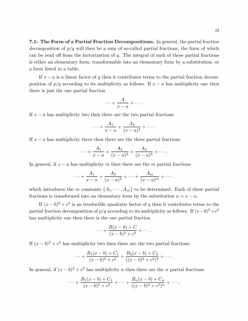
7.1: The Form of a Partial Fraction Decompositions. In general, the partial fraction
decomposition of p/q will then be a sum of so-called partial fractions, the form of which
can be read off from the factorization of q. The integral of each of these partial fractions
is either an elementary form, transformable into an elementary form by a substitution, or
a form listed in a table.
If x− a is a linear factor of q then it contributes terms to the partial fraction decom-
position of p/q according to its multiplicity as follows. If x − a has multiplicity one then
there is just the one partial fraction
· · ·+ A
x− a+ · · · .
If x− a has multiplicity two then there are the two partial fractions
· · ·+ A1
x− a+
A2
(x− a)2+ · · · .
If x− a has multiplicity three then there are the three partial fractions
· · ·+ A1
x− a+
A2
(x− a)2+
A3
(x− a)3+ · · · .
In general, if x− a has multiplicity m then there are the m partial fractions
· · ·+ A1
x− a+
A2
(x− a)2+ · · ·+ Am
(x− a)m+ · · · .
which introduces the m constants {A1, · · · , Am} to be determined. Each of these partial
fractions is transformed into an elementary form by the substitution u = x− a.
If (x− b)2 + c2 is an irreducible quadratic factor of q then it contributes terms to the
partial fraction decomposition of p/q according to its multiplicity as follows. If (x−b)2+c2
has multiplicity one then there is the one partial fraction
· · ·+ B(x− b) + C
(x− b)2 + c2+ · · · .
If (x− b)2 + c2 has multiplicity two then there are the two partial fractions
· · ·+ B1(x− b) + C1
(x− b)2 + c2+
B2(x− b) + C2
((x− b)2 + c2)2+ · · · .
In general, if (x− b)2 + c2 has multiplicity n then there are the n partial fractions
· · ·+ B1(x− b) + C1
(x− b)2 + c2+ · · ·+ Bn(x− b) + Cn
((x− b)2 + c2)n+ · · · ,
24
which introduces the 2n constants {B1, C1, · · · , Bn, Cn} to be determined. Each of these
partial fractions that is multiplied by the constants {B1, · · · , Bn} is transformed into an
elementary form by the substitution u = (x− b)2 + c2. The partial fraction multiplied by
the constant C1 is exactly the irreducible case that was treated in Section 1.2. Each of
these partial fractions that is multiplied by the constants {C2, · · · , Cn} will be found in
any table of integrals.
The total number of constants introduced in this way by all the factors of q will
be equal to deg(q). For instance, assuming that deg(p) < deg(q), and that the factors
of each q denoted with different lower-case letters are distinct, we have partial fraction
decompositions of the form
p(x)
(x− a)(x− b)(x− c)=
A
x− a+
B
x− b+
C
x− c,
p(x)
(x− a)(x− b)2=
A
x− a+
B
x− b+
C
(x− b)2,
p(x)
(x− a)3=
A
x− a+
B
(x− a)2+
C
(x− a)3,
p(x)
(x− a)((x− b)2 + c2)=
A
x− a+
B(x− b) + C
(x− b)2 + c2,
p(x)
(x− a)2((x− b)2 + c2)=
A
x− a+
B
(x− a)2+
C(x− b) +D
(x− b)2 + c2,
p(x)
(x− a)((x− b)2 + c2)2=
A
x− a+
B(x− b) + C
(x− b)2 + c2+
D(x− b) +E
((x− b)2 + c2)2.
The first four examples list all the combinations of factors that can arise when q is a cubic
polynomial, and consequently three constants {A,B,C} are introduced. In the fifth and
sixth examples the q are quartic and quintic, and consequently four constants {A,B,C,D}and five constants {A,B,C,D,E} are introduced respectively.
7.2: Determination of the Constants for Linear Factors. The constants associated
with any linear factor (x − a) in a partial fraction decomposition can be determined any
number of ways. The best is an extension of the method of matching residuals that was
introduced for the case where q was quadratic.
First we consider the case when (x − a) has multiplicity one. The partial fraction
decomposition then has the form
p(x)
q(x)=
A
x− a+ s(x) ,
where s(x) denotes all the partial fractions associated with other factors of q. Let r be the
residual of p/q associated with the factor (x−a) — namely, the rational function obtained
25
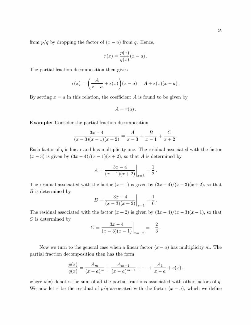
from p/q by dropping the factor of (x− a) from q. Hence,
r(x) =p(x)
q(x)(x− a) .
The partial fraction decomposition then gives
r(x) =
(
A
x− a+ s(x)
)
(x− a) = A+ s(x)(x− a) .
By setting x = a in this relation, the coefficient A is found to be given by
A = r(a) .
Example: Consider the partial fraction decomposition
3x− 4
(x− 3)(x− 1)(x+ 2)=
A
x− 3+
B
x− 1+
C
x+ 2.
Each factor of q is linear and has multiplicity one. The residual associated with the factor
(x− 3) is given by (3x− 4)/(x− 1)(x+ 2), so that A is determined by
A =3x− 4
(x− 1)(x+ 2)
∣
∣
∣
∣
x=3
=1
2.
The residual associated with the factor (x− 1) is given by (3x− 4)/(x− 3)(x+2), so that
B is determined by
B =3x− 4
(x− 3)(x+ 2)
∣
∣
∣
∣
x=1
=1
6.
The residual associated with the factor (x+2) is given by (3x− 4)/(x− 3)(x− 1), so that
C is determined by
C =3x− 4
(x− 3)(x− 1)
∣
∣
∣
∣
x=−2
= −2
3.
Now we turn to the general case when a linear factor (x− a) has multiplicity m. The
partial fraction decomposition then has the form
p(x)
q(x)=
Am
(x− a)m+
Am−1
(x− a)m−1+ · · ·+ A1
x− a+ s(x) ,
where s(x) denotes the sum of all the partial fractions associated with other factors of q.
We now let r be the residual of p/q associated with the factor (x − a), which we define
26
to be the rational function obtained from p/q by dropping the factor of (x− a)m from q.
Hence,
r(x) =p(x)
q(x)(x− a)m .
The partial fraction decomposition then gives
r(x) =
(
Am
(x− a)m+
Am−1
(x− a)m−1+ · · ·+ A1
x− a+ s(x)
)
(x− a)m
= Am + Am−1(x− a) + · · ·+ A1(x− a)m−1 + s(x)(x− a)m .
On the other hand, the Taylor approximation of r at a gives
r(x) = r(a) + r′(a)(x− a) + · · ·+ 1
(m− 1)!r(m−1)(a)(x− a)m−1 + · · · .
The coefficients {Am, · · · , A1} can then be read off as
Am = r(a) , Am−1 = r′(a) , · · · A1 =1
(m− 1)!r(m−1)(a) ,
which can be expressed more compactly as
Am−k =1
k!r(k)(a) , for k = 0, 1, · · · , m− 1 .
If you do not know the Taylor approximation yet, just memorize the formula above.
Example: Consider the partial fraction decomposition
3x− 4
(x− 3)(x+ 2)3=
A
x− 3+
B
x+ 2+
C
(x+ 2)2+
D
(x+ 2)3.
The factor x−3 has multiplicity one and the associated residual is given by (3x−4)/(x+2)3,
so that A is determined by
A =3x− 4
(x+ 2)3
∣
∣
∣
∣
x=3
=1
25.
The factor x + 2 has multiplicity three and the associated residual is given by r(x) =
(3x− 4)/(x− 3), whereby
r′(x) =−5
(x− 3)2, r′′(x) =
10
(x− 3)3,
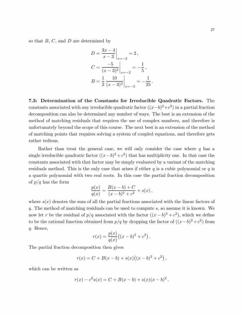
27
so that B, C, and D are determined by
D =3x− 4
x− 3
∣
∣
∣
∣
x=−2
= 2 ,
C =−5
(x− 3)2
∣
∣
∣
∣
x=−2
= −1
5,
B =1
2
10
(x− 3)3
∣
∣
∣
∣
x=−2
= − 1
25.
7.3: Determination of the Constants for Irreducible Quadratic Factors. The
constants associated with any irreducible quadratic factor ((x−b)2+c2) in a partial fraction
decomposition can also be determined any number of ways. The best is an extension of the
method of matching residuals that requires the use of complex numbers, and therefore is
unfortunately beyond the scope of this course. The next best is an extension of the method
of matching points that requires solving a system of coupled equations, and therefore gets
rather tedious.
Rather than treat the general case, we will only consider the case where q has a
single irreducible quadratic factor ((x−b)2+c2) that has multiplicity one. In that case the
constants associated with that factor may be simply evaluated by a variant of the matching
residuals method. This is the only case that arises if either q is a cubic polynomial or q is
a quartic polynomial with two real roots. In this case the partial fraction decomposition
of p/q has the formp(x)
q(x)=
B(x− b) + C
(x− b)2 + c2+ s(x) ,
where s(x) denotes the sum of all the partial fractions associated with the linear factors of
q. The method of matching residuals can be used to compute s, so assume it is known. We
now let r be the residual of p/q associated with the factor ((x− b)2 + c2), which we define
to be the rational function obtained from p/q by dropping the factor of ((x−b)2+c2) from
q. Hence,
r(x) =p(x)
q(x)
(
(x− b)2 + c2)
.
The partial fraction decomposition then gives
r(x) = C +B(x− b) + s(x)(
(x− b)2 + c2)
,
which can be written as
r(x)− c2s(x) = C +B(x− b) + s(x)(x− b)2 .
28
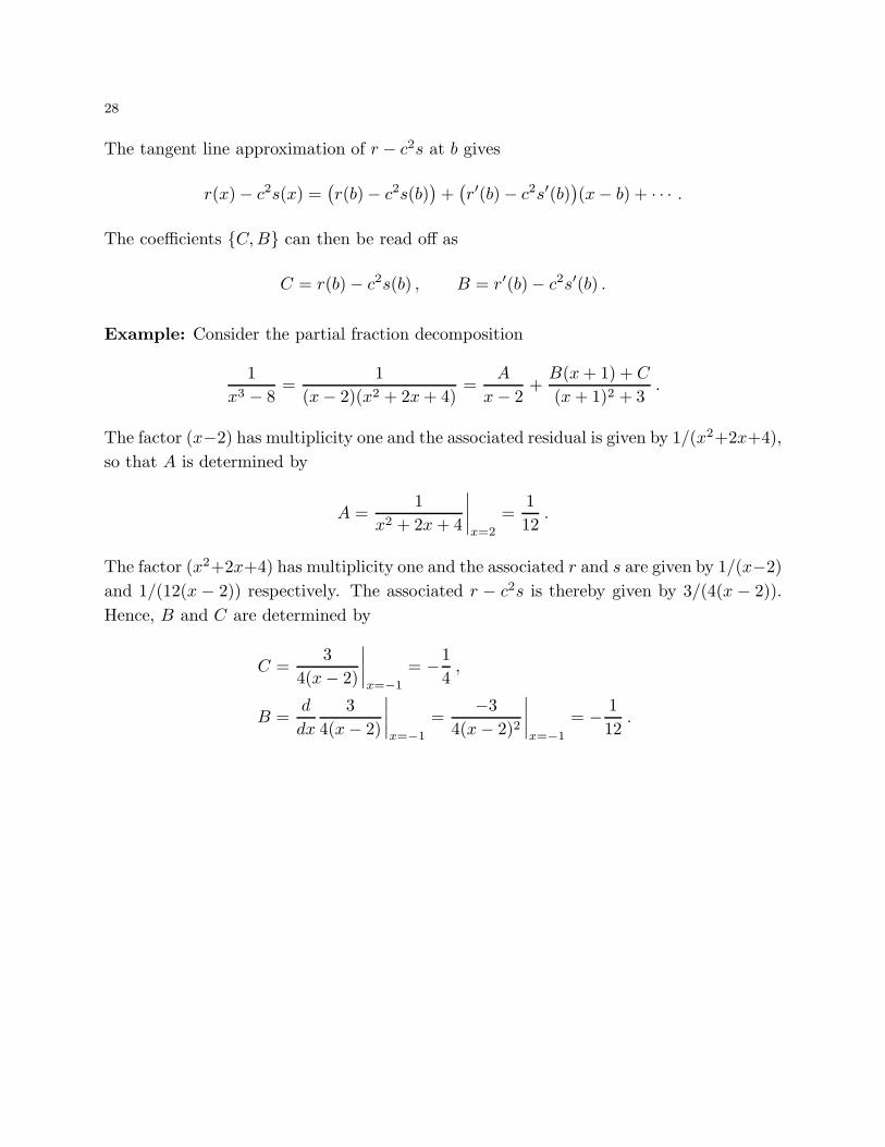
The tangent line approximation of r − c2s at b gives
r(x)− c2s(x) =(
r(b)− c2s(b))
+(
r′(b)− c2s′(b))
(x− b) + · · · .
The coefficients {C,B} can then be read off as
C = r(b)− c2s(b) , B = r′(b)− c2s′(b) .
Example: Consider the partial fraction decomposition
1
x3 − 8=
1
(x− 2)(x2 + 2x+ 4)=
A
x− 2+
B(x+ 1) + C
(x+ 1)2 + 3.
The factor (x−2) has multiplicity one and the associated residual is given by 1/(x2+2x+4),
so that A is determined by
A =1
x2 + 2x+ 4
∣
∣
∣
∣
x=2
=1
12.
The factor (x2+2x+4) has multiplicity one and the associated r and s are given by 1/(x−2)
and 1/(12(x − 2)) respectively. The associated r − c2s is thereby given by 3/(4(x − 2)).