HOW TO LOCALIZE TEN MICROPHONES IN ONE FINGER SNAP

Ivan Dokmanic †, Laurent Daudet ‡ and Martin Vetterli †

†School of Computer and Communication SciencesEcole Polytechnique Federale de Lausanne (EPFL),

CH-1015 Lausanne, Switzerland{ivan.dokmanic, martin.vetterli}@epfl.ch

‡Institut LangevinESPCI, Universite Paris Diderot,

10 Rue Vauquelin 75005 Paris, Francelaurent.daudet@espci.fr

ABSTRACT

A compelling method to calibrate the positions of micro-phones in an array is with sources at unknown locations.Remarkably, it is possible to reconstruct the locations of boththe sources and the receivers, if their number is larger thansome prescribed minimum [1, 2]. Existing methods, basedon times of arrival or time differences of arrival, only exploitthe direct paths between the sources and the receivers. In thisproof-of-concept paper, we observe that by placing the wholesetup inside a room, we can reduce the number of sourcesrequired for calibration. Moreover, our technique allows us tocompute the absolute position of the microphone array in theroom, as opposed to knowing it up to a rigid transformation orreflection. The key observation is that echoes correspond tovirtual sources that we get “for free”. This enables endeavorssuch as calibrating the array using only a single source.

Index Terms— Localization, array calibration, indoorcalibration, echo sorting, microphone array

1. INTRODUCTION

Most applications of microphone arrays require us to knowtheir relative positions. We are interested in two big groups ofapplications. First group is ad-hoc microphone arrays. Thiscould be microphones that are deployed to run an experimentor make a recording, or an array of microphones on devicesthat happen to share the room (smartphones, tablets, laptops,glasses). Another relevant group of applications is in verylarge, fixed microphone arrays, where precise hand measure-ments of the microphone positions become impossible. Byvery large we think of at least several tens, or even hundredsor thousands of microphones [3].

In the recent years, a number of methods were developedfor automatic position calibration of ad-hoc microphone ar-rays. These methods replace slow, imprecise and impracticalhand measurements. Some methods use specialized devices,such as loudspeakers mounted on a fixed construction [4], orassume partial knowledge of the array geometry.

This work was supported by an ERC Advanced Grant – Support forFrontier Research – SPARSAM Nr: 247006.

An interesting class of methods perform the calibrationwith sources at unknown positions. Authors in [5] formulatea non-linear least squares problem using at least five loud-speakers, and derive a closed form solution in the case whenone loudspeaker is close to a microphone. In [6], the authorsdemonstrate an approach that uses low-rank matrix factoriza-tion. When one microphone and one source are collocated,they too derive a closed-form expression for microphone posi-tions. With sources appearing at known times (as the authorsassume), the problem reduces to multi-dimensional unfold-ing, and the solution is similar to that in [7].

Some methods can additionally handle unknown offsettimes. Thrun [8] reported a matrix factorization based methodthat assumes the sources to be in the far-field. No far-fieldassumption is exhibited in [1] and [2]. In [2] the authors alsoallow for unknown internal delays of the microphone process-ing chain. Not knowing when the sources appeared prohibitsus from directly accessing the absolute distances between thesources and the microphones.

In the existing approaches, the room reverberation is ei-ther ignored or considered detrimental. We demonstrate thatbeing in a room facilitates the calibration, even if we do notknow how the room looks like or how the microphone arrayis positioned and oriented inside the room. We achieve thisby observing that the echoes correspond to virtual or imagesources, that we can exploit after correctly assigning them towalls.

It is somewhat surprising to note that the echoes help inthe calibration despite not knowing where they are comingfrom. Supposing that the positions of the walls are unknown,the location of the source is unknown, and the locations ofall the microphones are unknown, we are still able to esti-mate all these parameters. Particularly useful byproducts ofour algorithm are partial or complete information about theroom shape (as we also localize virtual sources), and the ar-ray’s absolute position in the room, not available with othercalibration methods. The proposed procedure is in a way atotal calibration—we learn about microphones, sources andreflectors. We show through numerical simulations that thealgorithm can indeed localize ten microphones with a singlesound source.

Microphone arrayAc

oust

ic e

vent

s

Src iMic j

timeSrc i

τi

Fig. 1: Calibration without echoes.

2. USING ECHOES FOR CALIBRATION

2.1. Anechoic Calibration

As a building block in our approach, we use an algorithm foranechoic calibration. Any of the algorithms mentioned in theintroduction will do. Consider the situation as in Fig. 1, andassume that the sources produce some impulsive sound thatthe microphones record, and whose time-of-arrival (TOA) wecan estimate (up to a possibly unknown offset). Assume fur-ther that the microphones are synchronized.

We denote the source positions by {sk}Kk=1, and the mi-crophone positions by {rm}Mm=1. An offset time τk is associ-ated with the kth source. Then we can express the measure-ments as

ϑkm = c τk + ‖sk − rm‖2. (1)

We collect the measurements in a matrix Θ =[ϑkm

]K,M

k,m=1.

As announced, we assume the existence of a module,a black box as far as we are concerned, that we denoteCalibrate, and that computes the estimates of the unknownmicrophone and source locations R

def= [r1, . . . , rM ],S

def=

[s1, . . . , sK ], and offsets τ = [τ1, . . . , τK ]T from Θ. Wecan write

(R, S, τ , ε) = Calibrate(Θ), (2)

where ε ≥ 0 denotes some measure of fit. The measure offit is computed as the discrepancy between the measured dataand the data that would have been generated by sensors atestimated positions,

ε =

K∑k=1

M∑m=1

|ϑkm − (‖sk − rm‖2 + c τk)|2 (3)

If R, S and τ perfectly generate Θ, then ε = 0.Any algorithm behind the Calibrate component is asso-

ciated with a certain minimal number of microphones andsources required for estimation, call them Mmin and Kmin.Often, Kmin is a (non-increasing) function of Mmin. A par-ticular consequence of this is that the minimal number of

Microphone arrayAc

oust

ic e

vent

s

Mic j

Wall

Virtu

al a

cous

tic e

vent

s

timeSrc i

τi

Src i

Virtual src i

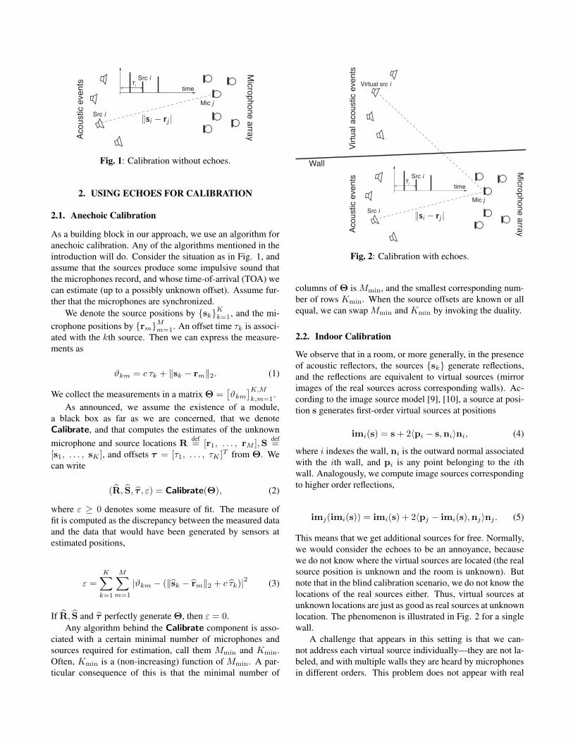
Fig. 2: Calibration with echoes.

columns of Θ is Mmin, and the smallest corresponding num-ber of rows Kmin. When the source offsets are known or allequal, we can swap Mmin and Kmin by invoking the duality.

2.2. Indoor Calibration

We observe that in a room, or more generally, in the presenceof acoustic reflectors, the sources {sk} generate reflections,and the reflections are equivalent to virtual sources (mirrorimages of the real sources across corresponding walls). Ac-cording to the image source model [9], [10], a source at posi-tion s generates first-order virtual sources at positions

imi(s) = s + 2〈pi − s,ni〉ni, (4)

where i indexes the wall, ni is the outward normal associatedwith the ith wall, and pi is any point belonging to the ithwall. Analogously, we compute image sources correspondingto higher order reflections,

imj(imi(s)) = imi(s) + 2〈pj − imi(s),nj〉nj . (5)

This means that we get additional sources for free. Normally,we would consider the echoes to be an annoyance, becausewe do not know where the virtual sources are located (the realsource position is unknown and the room is unknown). Butnote that in the blind calibration scenario, we do not know thelocations of the real sources either. Thus, virtual sources atunknown locations are just as good as real sources at unknownlocation. The phenomenon is illustrated in Fig. 2 for a singlewall.

A challenge that appears in this setting is that we can-not address each virtual source individually—they are not la-beled, and with multiple walls they are heard by microphonesin different orders. This problem does not appear with real

calibration events, as they are well separated in time. We needto label the echoes by performing echo sorting, introduced in[11]. There, the need to disambiguate echoes (virtual sources)arises when estimating the shape of a room from sound. How-ever, the problems are not the same—in the scenario therein,the authors assume they know the relative geometry of the mi-crophone array. In the calibration problem, we do not knowit. This means that the minimal number of microphones andthe minimal number of sources will be higher, as reflected byKmin and Mmin.

The principle at play is similar to the one used in [11]:Provided we have enough noiseless measurements ϑkm, theequations (1) yield a unique solution for locations and offsets.That is, these are the only R, S and τ that could have gener-ated Θ. Depending on the solution strategy (e.g. solving anoptimization program), any wrong permutation or assignmentof echoes will lead to an unsolvable system (1), or will yielda wrong solution that cannot recreate the measurements Θ.

The goal is to find the best fit among all possible echoassignments. This can be achieved by running Calibrate fordifferent echo assignments, and taking as the correct assign-ment the one with the smallest ε. The described procedure issummarized in Algorithm 1.

Performing the combinatorial search is feasible for smallarray sizes. For large arrays, however, the number of combi-nations becomes too big, and we need to do something else.In this case, we can bootstrap the method by first running itfor one or more sub-arrays of the big array. Depending on thetarget application, we might even have an idea about groupsof microphones that are spatially close (this will be the casefor large fixed arrays). Knowing which microphones are closein space is relevant, as proximity makes it more likely that themicrophones will have picked up the same echoes. In spa-tially large arrays, it is not guaranteed that all the microphoneswill hear all the echoes.

The estimation can be performed one acoustic event at atime (e.g. a finger snap). This is useful, as we know thatthe time offset τ will be the same for all virtual events cor-responding to a single real event (and it will be equal to theoffset of that event). Structured information like this can beexploited in the design of the Calibrate module.

2.3. Minimal Infrastructure for Calibration

We can use a degree-of-freedom counting argument as in [2]to determine the smallest number of microphones and sourcesnecessary for the calibration. Every microphone brings inthree unknowns (x, y and z coordinates), while every sourcebrings in four unknowns (coordinates and the offset τ ). Onthe other hand, every source gives us M TOA measurements.The total number of measurements is then MK, and we needthis number to be larger than the total number of unknowns,3M+4K. Note further that we can fix the location of one mi-crophone and the rotation of the remaining points around thismicrophone. This takes out a total of six degrees of freedom,

Algorithm 1 BASIC INDOOR CALIBRATION

Input: � Microphone recorded signals {ym(t)}Mm=1

Output: � Estimated microphone positions R

� Estimated source positions S� Estimated source offsets τ

Peak picking:

� For every ym(t) find the set of peaks (echoes), Tm

Initialization:

� εbest ←∞

For every feasible echo assignment across {Tm}:

� Create the corresponding matrix Θi

� (R, S, τ , ε) = Calibrate(Θi)

� If (ε < εbest), then (Rbest,Sbest, τbest, εbest) ←(R, S, τ , ε)

End For

resulting finally in

K ≥⌈3M − 6

M − 4

⌉. (6)

The only remaining ambiguity is the 1-bit reflection ambigu-ity. The relationship between the minimal number of micro-phones and sources is always a property of the method usedto calibrate.

We use this example to show that something remarkablecan happen in a room. Suppose that M = 10. In this case,we compute that K ≥ 4—we need at least four sources. Nowimagine that in a room we have a single acoustic event, andthat we can get at least three echoes. Together with the di-rect sound, we get enough measurements (real and virtual) toactually calibrate the microphone array, and to determine itsabsolute orientation with respect to the walls. This is true inspite of the fact that we do not know the room, the micro-phone locations, the source location nor the source timing. Inthis case we only need to estimate a single emission time, asit will be the same for all the image sources.

3. PRACTICAL ALGORITHM

3.1. Reducing the number of combinations

The main drawback of the proposed algorithm is the com-binatorial search. Especially in the case of large arrays, thenumber of combinations becomes too large to test them all.The following heuristics can be employed in order to reducethe number of combinations,

i) Perform the estimation for sub-arrays,ii) Combine the echoes only within a temporal window

corresponding to the array size,

Distances between pairs of microphones

Source-microphonedistances

Sour

ce-m

icro

phon

edi

stan

ces

Sourcedists.

Fig. 3: Structure of the EDM used to fine-tune the estimate.

iii) Assume only a small number of echo swaps can occurper microphone,

iv) Assume echo swaps occurred at a limited number ofmicrophones,

v) Normalize by the decay and discriminate first-orderpeaks by the magnitude,

vi) Order the echo assignments by the likelihood and stopas soon as we get a score below a prescribed threshold.

3.2. Dealing with Noise

For the numerical experiments in this paper, we implementedthe Calibrate module based on [1]. A nice feature of thatalgorithm is that in its basic version it is fast, and it gives agood initial estimate of the unknown times and locations.

To further optimize the estimate, we propose an iterativealgorithm based on Euclidean distance matrices (EDM) [12]and multi-dimensional scaling (MDS) [13].

Let {xi}m+ni=1 list the points corresponding to sources and

to microphones, so that xi = ri for 1 ≤ i ≤ M and xi =si−M for (M + 1) ≤ i ≤ (M + K). Denote by D theEuclidean distance matrix (EDM) corresponding to the pointset {xi}, that is, D = (dij), where dij = ‖xi − xj‖2. Thestructure of D is illustrated in Fig. 3.

The main ingredient of the solution is an algorithm forMDS. MDS aims to embed a set of points in Rn given theirnoisy pairwise distances. Among the many approaches toMDS we choose to minimize the cost function called s-stress.Given a noisy EDM D, we obtain a denoised matrix as

MDS(D)def= argmin

D∈EDM3

∑ij

(d 2ij − d 2

ij

)2. (7)

By EDM3 we denote the set of EDMs generated by point setsin 3D. This cost function is not convex. Nevertheless, it wasshown that a coordinate-alternating approach to minimizationalmost always achieves the global optimum [14].

Algorithm 2 EDM-BASED UNFOLDING

Input: � Initial source-microphone distances� Initial inter-microphone distances

Output: � Estimates of {sk}Kk=1 and {rm}Mi=m

Initialization:� Construct the matrix D from the input data (source-

microphone distances into the shaded part, and inter-microphone, and inter-source distances in the non-shaded parts)

Repeat� Set the elements of D corresponding to source-mic dis-

tances to input values (shaded regions in Fig. 3)� Find the closest EDM to D, D← argmin s(D)

Until convergence

� Estimate the positions of points generating D as

{xi}M+Ki=1 = argmin

{xi∈R3}

∑ij

(‖xi − xj‖2 − d 2

ij

)2, and

extract R and S

We assume that the source-microphone distances weremore accurately estimated than the inter-microphone dis-tances. Thus the iteration of the proposed algorithm consistsin enforcing the elements of the matrix corresponding tosource-microphone distances, and then relaxing the matrixusing MDS. We empirically observe that the described proce-dure (Algorithm 2) considerably improves the initial estimate.

4. NUMERICAL EXPERIMENT—SINGLE SOURCE

We ran numerical simulations using only one acoustic eventto localize ten microphones. In this case, all of the sources(real or virtual) have the same offset τ .

We simulated a shoebox room with dimensions W = 5m, L = 6 m, H = 3 m, using the image source model, upto second-order reflections. We experimented with randommicrophone array geometries and with different numbers ofmicrophones. The algorithm used for echo sorting and for thefinal reconstruction is the combination described in Section3. Room acoustics were simulated using the image sourcemodel up to second-order reflections, and the first six echoeswere used for estimation.

Simulations confirm that it is possible to obtain accurateestimates of microphone positions by using only a singlesource. The room shape or dimensions are considered un-known by the algorithm. Despite this, we obtain a fullreconstruction of the source and microphone locations, aswell as their absolute pose inside the room (more precisely,relative to the localized image sources). We also obtain thepositions of walls corresponding to these image sources. Tworeconstruction examples are shown in Fig. 4 (A) and (B), forrandom microphone arrays comprising ten microphones. Fig.

0 0.5 1 1.5 20

0.05

0.1

0.15

0.2

Largest pulse jitter [cm]

Roo

t Mea

n Sq

uare

d Er

ror [

cm]

10 microphones20 microphones

A B C

Fig. 4: (A) and (B) Two typical reconstruction results with M = 10 microphones randomly placed inside a box approximately1m × 1m × 0.5m large. We emphasize that the room dimensions (5m × 6m × 3m) and the room shape is not assumed known.Red-black triangle represents the source location. Small black crosses are true microphone locations, while blue squares denotethe estimated locations. (C) Accuracy of microphone localization with jittered pulses. The jitter that was added to pulses wasdrawn from U [−d, d], where d is indicated on the abscissa in [cm]. The room was of the same dimensions as in (A) and (B).

4 (C) shows the root-mean-squared error for the estimates ofmicrophone positions against the amount of jitter. It can beseen that the algorithm performs stably in moderate jitter.

5. CONCLUSION

We presented the proof-of-concept of constructive use ofechoes for microphone array calibration. Interpreting echoesas virtual sources allows us to reduce the number of sourcesrequired to calibrate the array. In the extreme case, it ispossible to calibrate using only a single acoustic event suchas a finger snap, even without knowing the room. To thebest of our knowledge, this is the first description of such apossibility.

The main line of future work concerns reducing the num-ber of echo assignments to test. Furthermore, we intend to de-sign Calibrate modules adapted for the specific case of equaltime offsets.

References[1] M. Pollefeys and D. Nister, “Direct computation of

sound and microphone locations from time-difference-of-arrival data,” in Proc. IEEE Intl. Conf. on Acoust.,Speech and Signal Process., Las Vegas, 2008, pp. 2445–2448, IEEE.

[2] N. D. Gaubitch, W. B. Kleijn, and R. Heusdens, “Auto-localization in ad-hoc microphone arrays,” in Proc.IEEE Intl. Conf. on Acoust., Signal and Speech Process.,Vancouver, 2013, pp. 106–110, IEEE.

[3] E. Weinstein, K. Steele, A. Agarwal, and J. Glass,“LOUD: A 1020-node microphone array and acousticbeamformer,” in International Congress on Sound andVibration, 2007.

[4] J. M. Sachar, H. F. Silverman, and W. R. Patterson,“Microphone position and gain calibration for a large-

aperture microphone array,” IEEE Trans. Speech AudioProcess., vol. 13, no. 1, pp. 42–52, Jan. 2005.

[5] V. C. Raykar and R. Duraiswami, “Automatic positioncalibration of multiple microphones,” in Proc. IEEEIntl. Conf. on Acoust., Signal and Speech Process., Mon-treal, 2004, pp. 69–72, IEEE.

[6] M. Crocco, A. D. Bue, and V. Murino, “A Bilinear Ap-proach to the Position Self-Calibration of Multiple Sen-sors,” IEEE Trans. Signal Process., vol. 60, no. 2, pp.660–673, 2012.

[7] P. H. Schonemann, “On metric multidimensional un-folding,” Psychometrika, vol. 35, no. 3, pp. 349–366,1970.

[8] S. Thrun, “Affine Structure From Sound,” in Proc. Conf.Neural Inf. Process. Sys. (NIPS), Cambridge, MA, 2005,MIT Press.

[9] J. B. Allen and D. A. Berkley, “Image Method For Ef-ficiently Simulating Small-room Acoustics,” J. Acoust.Soc. Am., vol. 65, no. 4, pp. 943–950, 1979.

[10] J. Borish, “Extension of the Image Model To ArbitraryPolyhedra,” J. Acoust. Soc. Am., vol. 75, no. 6, pp.1827–1836, 1984.

[11] I. Dokmanic, R. Parhizkar, A. Walther, Y. M. Lu, andM. Vetterli, “Acoustic echoes reveal room shape,” Proc.Natl. Acad. Sci., vol. 110, no. 30, June 2013.

[12] J. Dattorro, Convex Optimization & Euclidean DistanceGeometry, Meboo, 2011.

[13] W. S. Torgerson, “Multidimensional scaling: I. Theoryand method,” Psychometrika, vol. 17, no. 4, pp. 401–419, Dec. 1952.

[14] R. Parhizkar, Euclidean distance matrices: Properties,algorithms and applications, Ph.D. thesis, EPFL, Lau-sanne, 2013.