22
Evolutionary Genetics LV 25600-01 | Lecture with exercises | 6KP HS2017 Population subdivision “suburban sprawl”

Evolutionary Genetics
LV 25600-01 | Lecture with exercises | 6KP
HS2017
Population subdivision
“sub
urba
n sp
raw
l”

Population Genetics ▷ Subdivision
HS17 | UniBas | JCW 2
Non-Random Mating > Isolation by Distance > Subdivision
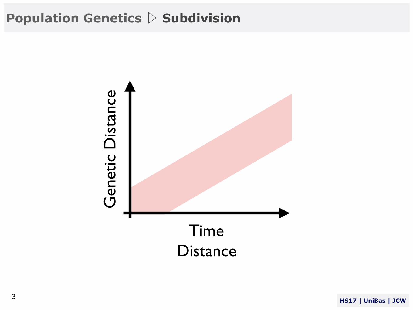
Population Genetics ▷ Subdivision
HS17 | UniBas | JCW 3
Time
Gen
etic
Dis
tanc
e
Distance

Population Genetics ▷ Subdivision
HS17 | UniBas | JCW 4
Expected increase in FST over time (generations) among completely isolated populations of different population sizes.
FST = 1− 1− 12Ne
⎛⎝⎜
⎞⎠⎟
t
Allendorf, Luikart, and Aitken (2013)

Population Genetics ▷ Subdivision
HS17 | UniBas | JCW 5
Forbes and Hogg (1999)

Population Genetics ▷ Subdivision
HS17 | UniBas | JCW 6

Population Genetics ▷ Subdivision
HS17 | UniBas | JCW 7
The oldest and most widely used metrics of genetic differentiation are Fstatistics. Sewall Wright (1931, 1951) developed a conceptual and mathematical framework to describe the distribution of genetic variation within a species that used a series of inbreeding coefficients: FIS, FST, and FIT.
Fstatistics were initially defined by Wright for loci with just two alleles. They were extended to three or more alleles by Nei (1977), who used the parameters GIS, GST, and GIT in what he termed the analysis of gene diversity. F and G statistics are often used interchangeably in the literature – see Chakraborty and Leimar (1987) for a comprehensive discussion of Fand Gstatistics. Masatoshi Nei
1931
Sewall Wright 1889-1988
Population Genetics ▷ Subdivision
HS17 | UniBas | JCW 8
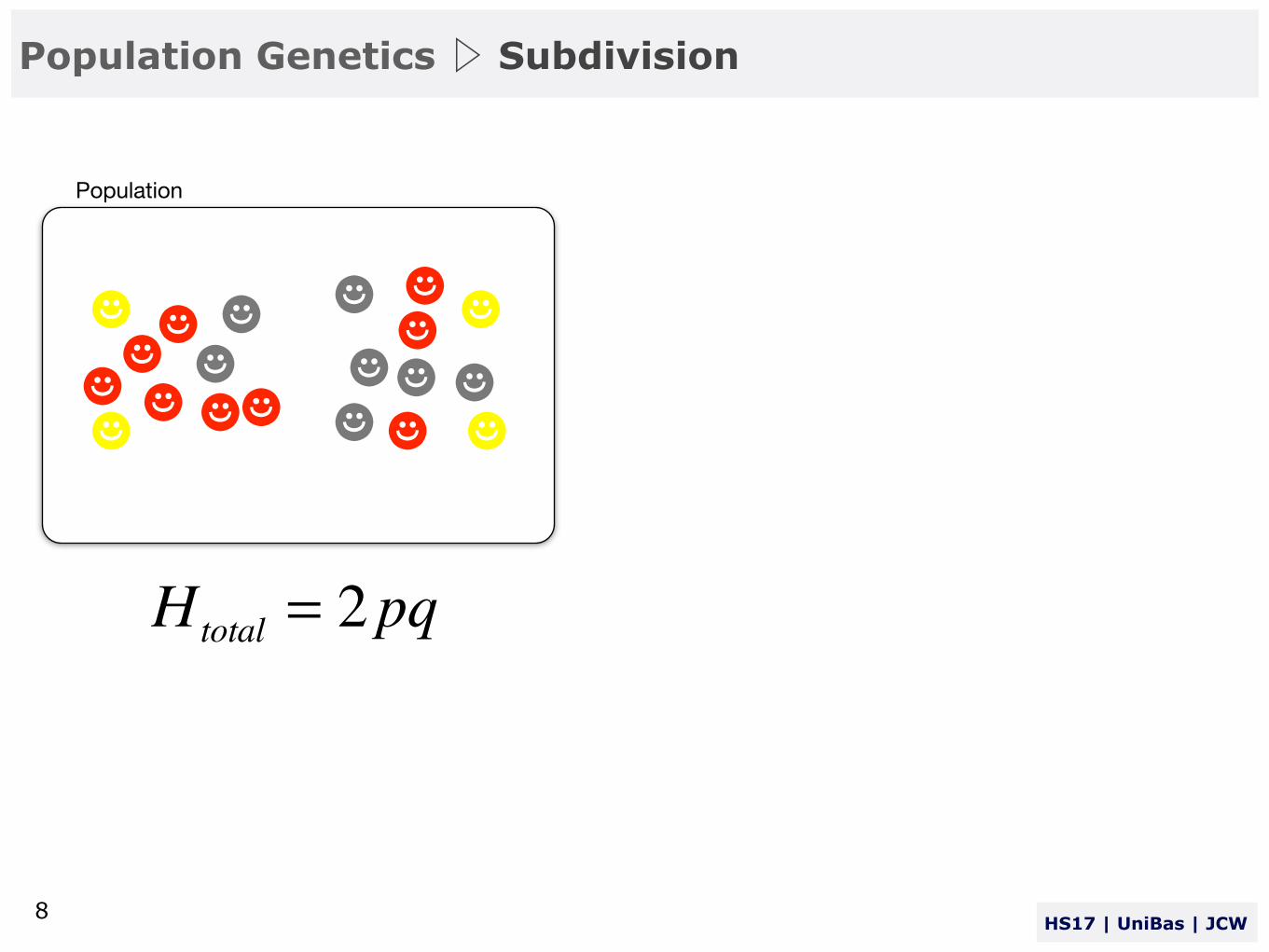
☻☻☻
☻☻☻ ☻
☻☻
☻☻☻☻
☻ ☻☻☻
☻☻ ☻
Htotal = 2pq
Population

Population Genetics ▷ Subdivision
HS17 | UniBas | JCW 9
☻☻☻
☻☻☻ ☻
☻☻
☻☻☻
West East
☻☻ ☻☻
☻
☻☻ ☻
Htotal = 2pq
Population - Subpopulations
West East
NA1A2
Nwest
NA1A2
Neast

Population Genetics ▷ Subdivision
HS17 | UniBas | JCW 12
☻☻☻
☻☻☻ ☻
☻☻
☻☻☻
West EastObserved average heterozygosity in subpopulations
HI =(#A1A2west/Nwest)+(#A1A2east/Neast)
2
Expected average heterozygosity assuming HWE
HS =(2pqwest)+(2pqeast)
2
Heterozygosity expected without subdivision
HT = 2pqtotal
☻☻ ☻☻
☻
☻☻ ☻
Htotal = 2pq
Population - Subpopulations
Population Genetics ▷ Subdivision
HS17 | UniBas | JCW 13
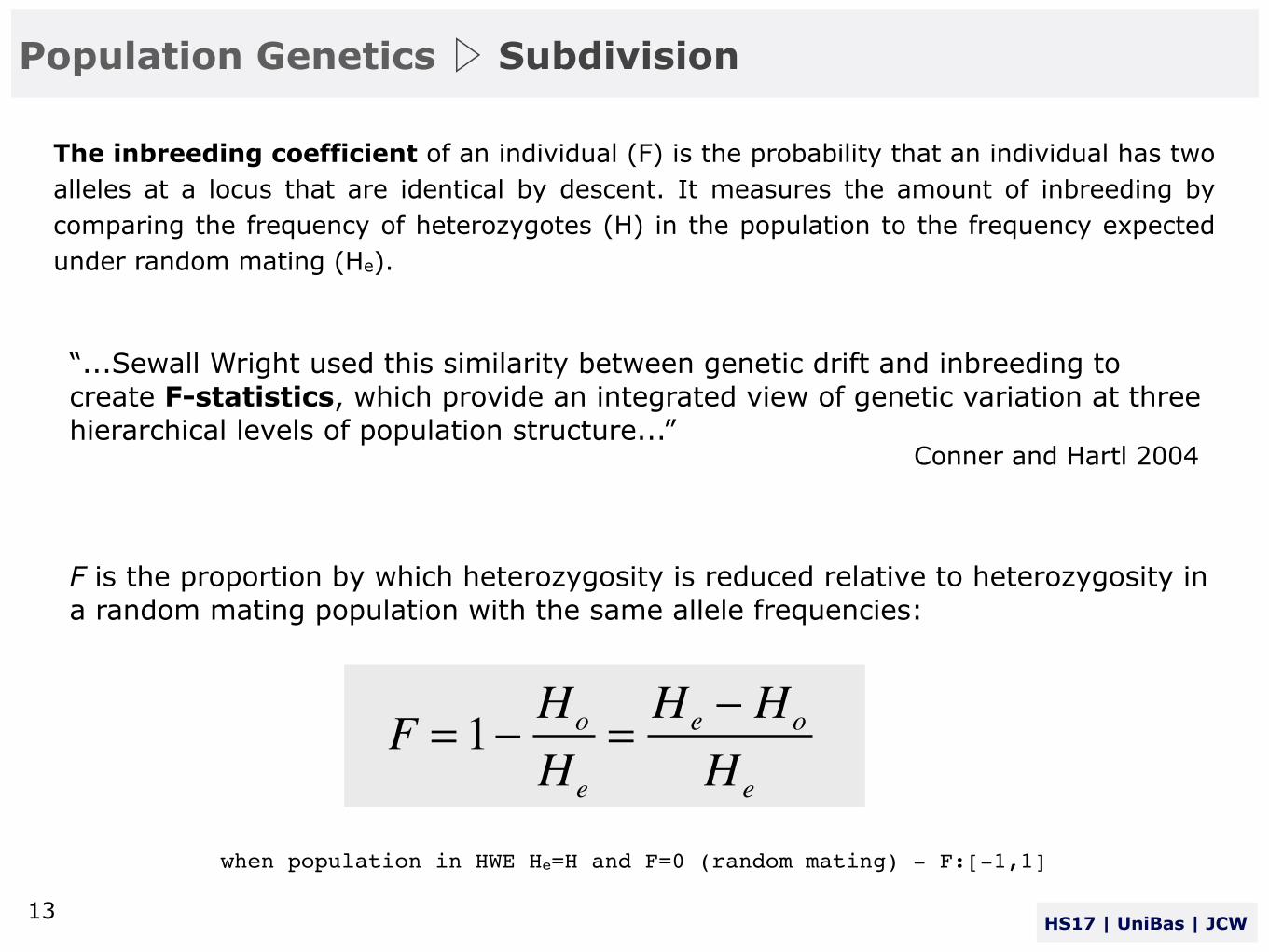
The inbreeding coefficient of an individual (F) is the probability that an individual has two alleles at a locus that are identical by descent. It measures the amount of inbreeding by comparing the frequency of heterozygotes (H) in the population to the frequency expected under random mating (He).
when population in HWE He=H and F=0 (random mating) - F:[-1,1]
F = 1− Ho
He
=He − Ho
He
“...Sewall Wright used this similarity between genetic drift and inbreeding to create F-statistics, which provide an integrated view of genetic variation at three hierarchical levels of population structure...”
Conner and Hartl 2004
F is the proportion by which heterozygosity is reduced relative to heterozygosity in a random mating population with the same allele frequencies:

Population Genetics ▷ Subdivision
HS17 | UniBas | JCW 14
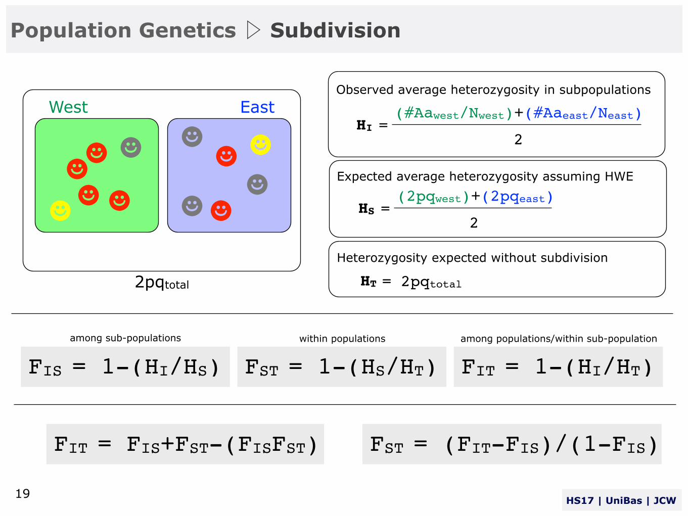
The different F-statistics look at different levels of population structure. FIT is the inbreeding coefficient of an individual (I) relative to the total (T) - FIS is the inbreeding coefficient of an individual (I) relative to the subpopulation (S) - and FST is the effect of subpopulations (S) compared to the total population (T).

Population Genetics ▷ Subdivision
HS17 | UniBas | JCW 17
FIS = 1-(HI/HS)...for individuals (I) within sub-population (S):
FST = 1-(HS/HT)...for sub-population (S) relative to metapopulation (T):
FIT = 1-(HI/HT)...for individuals (I) within the metapopulation (T):
FIS: That proportion of the total inbreeding within a population due to inbreeding within sub-populations.
FST: That proportion of the total inbreeding in a population due to differentiation among sub-populations.
FIT: The total inbreeding in a population due to both inbreeding within sub-populations, and differentiation among sub-populations.
HI=∑HIi/n: observed heterozygosity within subpopulations , HS=∑2piqi/n: is the expected herterozygosity with random mating, and HT=2pq: is the expected heterozygosity of individuals based on allele frequencies averaged with random mating.
The F statistics can be calculated using the relationship between heterozygosity and inbreeding. This allows F statistics to be determined from genetic markers (Nei 1977; de Jong et al. 1994).

Population Genetics ▷ Subdivision
HS17 | UniBas | JCW 18
Sewall Wright (1969) used inbreeding coefficient to describe the distribution of genetic diversity within and among population fragments; he partitioned total inbreeding of individuals (I) relative to the total (T) population (FIT) into that inbreeding of individuals relative to their sub-population (S), FIS and that dues to differentiation among sub-populations, relative to the total population FST.
FIT = FIS+FST-(FISFST)In words, the total inbreeding is the probability of identity by descent within fragments (FIS) plus the probability of identity by descent to subdivision (FST) minus the probability of identity by descent due to both.
FST = (FIT-FIS)/(1-FIS)
> FIT = FST+FIS-FISFST> 1-FIT = 1-FST-FIS+FISFST> (1-FIT) = (1-FIS)(1-FST)
> FIT = FST+FIS-FISFST> FIT = FIS+FST(1-FIS)> FST = (FIT-FIS)/(1-FIS)
Population Genetics ▷ Subdivision
HS17 | UniBas | JCW 19
FIS = 1-(HI/HS) FST = 1-(HS/HT) FIT = 1-(HI/HT)
☻☻☻
☻☻☻ ☻
☻☻
☻☻☻
West EastObserved average heterozygosity in subpopulations
HI =(#Aawest/Nwest)+(#Aaeast/Neast)
2
Expected average heterozygosity assuming HWE
HS =(2pqwest)+(2pqeast)
2
Heterozygosity expected without subdivision
HT = 2pqtotal2pqtotal
among sub-populations within populations among populations/within sub-population
FIT = FIS+FST-(FISFST) FST = (FIT-FIS)/(1-FIS)
Population Genetics ▷ Subdivision
HS17 | UniBas | JCW 20
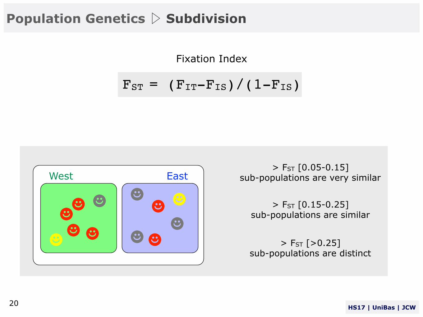
Fixation Index
> FST [0.05-0.15] sub-populations are very similar
> FST [0.15-0.25] sub-populations are similar
> FST [>0.25] sub-populations are distinct
FST = (FIT-FIS)/(1-FIS)
☻☻☻
☻☻☻ ☻
☻☻
☻☻☻
West East
Population Genetics ▷ Subdivision
HS17 | UniBas | JCW 21
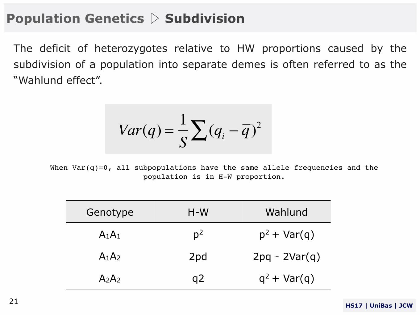
The deficit of heterozygotes relative to HW proportions caused by the subdivision of a population into separate demes is often referred to as the “Wahlund effect”.
Var(q) = 1S
(qi − q )2∑
When Var(q)=0, all subpopulations have the same allele frequencies and the population is in H-W proportion.
Genotype H-W Wahlund
A1A1 p2 p2 + Var(q)
A1A2 2pd 2pq - 2Var(q)
A2A2 q2 q2 + Var(q)
Population Genetics ▷ Subdivision
HS17 | UniBas | JCW 22
The Wahlund effect refers to reduction of heterozygosity in a population caused by subpopulation structure. Namely, if two or more subpopulations have different allele frequencies then the overall heterozygosity is reduced, even if the subpopulations themselves are in a Hardy-Weinberg equilibrium. The underlying causes of this population subdivision could be geographic barriers to gene flow followed by genetic drift in the subpopulations.
Wahlund, S. (1928). Zusammensetzung von Population und Korrelationserscheinung vom Standpunkt der Vererbungslehre aus betrachtet. Hereditas 11:65–106.
The Wahlund effect has a number of important consequences:
• We have to know about the structure of a population when applying the Hardy-Weinberg principle to it, otherwise there may seem to be more homozygotes than expected from the Hardy-Weinberg principle. We might then suspect that selection, or some other factor, was favouring homozygotes. In fact both sub-populations are in perfectly good Hardy-Weinberg equilibrium and the deviation is due to the unwitting pooling of the separate populations.
• A second consequence of the Wahlund effect is that when a number of previously subdivided populations merge together, the frequency of homozygotes will decrease. In humans, this can lead to a decrease in the incidence of rare recessive genetic diseases when a previously isolated population comes into contact with a larger population. The recessive disease is only expressed in the homozygous condition, and when the two populations start to interbreed, the frequency of those homozygotes goes down.

Population Genetics ▷ Subdivision
HS17 | UniBas | JCW 23
MORE T H I N G S CONSIDERED

Population Genetics ▷ Subdivision
HS17 | UniBas | JCW 24
http://www.evolution.unibas.ch/teaching/evol_genetics/3_Population_Genetics/reading/Holsinger_and_Weir_2009.pdf
Population Genetics ▷ Subdivision
HS17 | UniBas | JCW 25
In biology, a deme is a term for a local population of organisms of one species that actively interbreed with one another and share a distinct gene pool. When demes are isolated for a very long time they can become distinct subspecies or species. The term deme is mainly used in evolutionary biology and is often used as a synonym for population.
In evolutionary computation a "deme" often refers to any isolated subpopulation subjected to selection as a unit rather than as individuals.
A deme in biological evolution is conceptually related to a meme in cultural evolution, a term suggested by Richard Dawkins' 1976 book The Selfish Gene.
demeGreek dēmos, people, land; see d- in Indo-European roots.
(dēm)

Population Genetics ▷ Subdivision
HS17 | UniBas | JCW 26


