18
Huber smooth M-estimator
Huber smooth M-estimator
Mâra Vçliòa, Jânis Valeinis
University of Latvia
Sigulda, 28.05.2011
Mâra Vçliòa, Jânis Valeinis Huber smooth M-estimator

Huber smooth M-estimator
Contents
M-estimators
Huber estimator
Smooth M-estimator
Empirical likelihood method for M-estimators
Mâra Vçliòa, Jânis Valeinis Huber smooth M-estimator

Huber smooth M-estimator
Introduction
Aim: robust estimation of location parameter
Huber M-estimator (1964) - well known robust location
estimator
Owen (1988) introduced empirical likelihood method, also
applicable to M-estimators
Hampel (2011) proposed a smoothed version of Huber
estimator
Work in progress
Two sample problem: empirical likelihood based method for a
difference of smoothed Huber estimators
(Valeinis, Velina, Luta: abstract for ICORS 2011 conference)
Mâra Vçliòa, Jânis Valeinis Huber smooth M-estimator
Huber smooth M-estimator
M-estimators
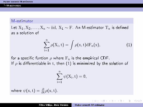
M-estimator
Let X1,X2, . . . ,Xn ∼ iid, X1 ∼ F. An M-estimator Tn is defined
as a solution of
n∑i=1
ρ(Xi, t) =
∫ρ(x, t)dFn(x), (1)
for a specific funtion ρ where Fn is the empirical CDF.
If ρ is differentiable in t, then (1) is minimized by the solution of
n∑i=1
ψ(Xi, t) = 0,
where ψ(x, t) = ∂∂tρ(x, t).
Mâra Vçliòa, Jânis Valeinis Huber smooth M-estimator
Huber smooth M-estimator
M-estimators
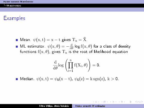
Examples
Mean. ψ(x, t) = x− t gives Tn = X̄.
ML estimator. ψ(x, θ) = − ddθ log f(x, θ) for a class of density
functions f(x, θ), gives Tn is the root of likelihood equation
d
dθlog
(n∏
i=1
f(Xi, θ)
)= 0.
Median. ψ(x, t) = ψ0(x− t), ψ0(z) = k sgn(z), k > 0.
Mâra Vçliòa, Jânis Valeinis Huber smooth M-estimator
Huber smooth M-estimator
Huber estimator
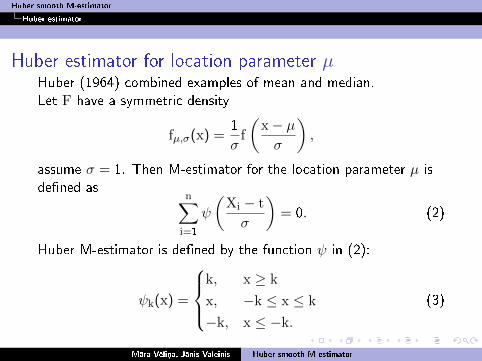
Huber estimator for location parameter µHuber (1964) combined examples of mean and median.
Let F have a symmetric density
fµ,σ(x) =1
σf
(x− µσ
),
assume σ = 1. Then M-estimator for the location parameter µ is
defined asn∑
i=1
ψ
(Xi − t
σ
)= 0. (2)
Huber M-estimator is defined by the function ψ in (2):
ψk(x) =
k, x ≥ k
x, −k ≤ x ≤ k
−k, x ≤ −k.(3)
Mâra Vçliòa, Jânis Valeinis Huber smooth M-estimator

Huber smooth M-estimator
Huber estimator
Huber's motivaton:
Unrestricted ψ-functions have undesired properties (unstable
to outliers);
Cosider the limiting values of k in ψk and their respectiveM-estimators:
If k→∞, then ψk is mean;If k→ 0, then ψk is median.
k is a tuning constant determining the degree of robustness.
Huber estimator has minimax assymptotic variance for class of
distribution functions
(1− ε)φ(x) + εh(x),
where φ is pdf of N(0, 1) and h is a symmetric density.
Mâra Vçliòa, Jânis Valeinis Huber smooth M-estimator
Huber smooth M-estimator
Huber estimator
Scaled estimator of location
In reality σ is not known, thus a robust estimate of σ should be
used. A common choice is MAD.
MAD
Sn = MAD = median(|Xi −median(Xi)|).
Robust estimator is acquired, even in presence of outliers (up to
50% of the sample).
Mâra Vçliòa, Jânis Valeinis Huber smooth M-estimator

Huber smooth M-estimator
Smooth M-estimator
Smoothed M-estimator (Hampel, 2011)
For a general ψ-function of an M-estimator define
ψ̃(x) =
∫ψ(x + u)dQn(u), (4)
where
Qn may be chosen as a the distribution of the initial
M-estimator
Qn can be approximated by N(0,V/n), where V is
assymptotic variance of the M-estimator.
Need to specify distribution under which the assymptotic
variance is computed.
The smoothing prinicple can be applied to ψ functions already
smooth.
Mâra Vçliòa, Jânis Valeinis Huber smooth M-estimator
Huber smooth M-estimator
Smooth M-estimator
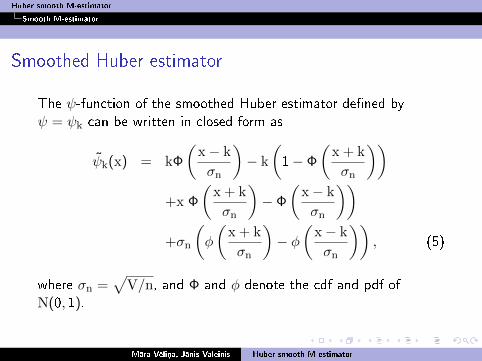
Smoothed Huber estimator
The ψ-function of the smoothed Huber estimator defined by
ψ = ψk can be written in closed form as
ψ̃k(x) = kΦ
(x− k
σn
)− k
(1− Φ
(x + k
σn
))+x Φ
(x + k
σn
)− Φ
(x− k
σn
))+σn
(φ
(x + k
σn
)− φ
(x− k
σn
)), (5)
where σn =√
V/n, and Φ and φ denote the cdf and pdf of
N(0, 1).
Mâra Vçliòa, Jânis Valeinis Huber smooth M-estimator
Huber smooth M-estimator
Smooth M-estimator
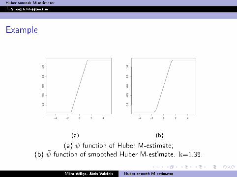
Example
−4 −2 0 2 4
−1.
0−
0.5
0.0
0.5
1.0
(a)
−4 −2 0 2 4
−1.
0−
0.5
0.0
0.5
1.0
(b)
(a) ψ function of Huber M-estimate;
(b) ψ̃ function of smoothed Huber M-estimate. k=1.35.
Mâra Vçliòa, Jânis Valeinis Huber smooth M-estimator

Huber smooth M-estimator
Empirical likelihood method for M-estimators
Empirical likelihood method for M-estimators
Owen (1988) showed that EL method can be applied to
certain M-estimators, including Huber estimator.
Nonparametric Wilk's theorem applies thus EL based
confidence intervals for Huber estimate can be obtained.
Tsao, Zhu (2001) showed that EL based confidence intervals
preserves robustness.
Mâra Vçliòa, Jânis Valeinis Huber smooth M-estimator

Huber smooth M-estimator
Empirical likelihood method for M-estimators
EL confidence bands for Huber estimator
Empirical likelihood ratio for parameter t
R(t) = sup{n∏
i=1
ωi
n∑i=1
ωiψ(Xi, t) = 0, ωi ≥ 0,
n∑i=1
ωi = 1}
is maximized by∏ωi(λ), where
ωi(λ) = {n(1 + λZi)}−1,
and Zi = ψ(Xi, t) and λ follows from
n−1∑
Zi/(1 + λZi) = 0.
Mâra Vçliòa, Jânis Valeinis Huber smooth M-estimator
Huber smooth M-estimator
Empirical likelihood method for M-estimators
−2 −1 0 1 2
05
1015
20
−2l
nL
EL vid.vertEL Huber
−2 −1 0 1 2 3 4 5
05
1015
20
−2l
nL
EL vid.vertEL Huber
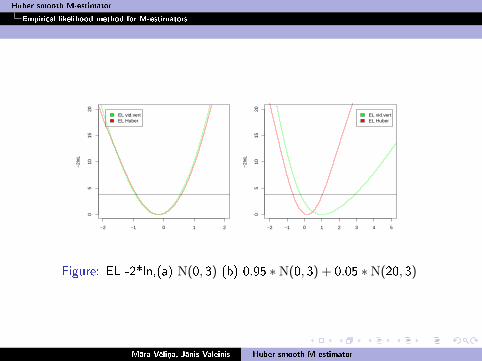
Figure: EL -2*ln,(a) N(0, 3) (b) 0.95 ∗N(0, 3) + 0.05 ∗N(20, 3)
Mâra Vçliòa, Jânis Valeinis Huber smooth M-estimator

Huber smooth M-estimator
Empirical likelihood method for M-estimators
Simulation results for one sample problem
Table: Huber estimation for location parameter and its EL confidencebands, alpha=0.05
N(0, 3) 0.95 ∗N(0, 3) + 0.05 ∗N(20, 3)
sample len estimate len estimate
n=50 EL.huber 0.494 EL.huber -0.055 EL.huber 1.706 EL.huber 0.159
EL.mean 0.492 EL.mean -0.064 EL.mean 3.14 EL.mean 1.008
t-test 0.506 mean -0.064 t-test 3.117 mean 1.008
z-test 0.554 huber -0.076 z-test 0.554 huber 0.159
Bootstrap 0.497 Bootstrap 3.057
n=20 EL.huber 0.667 EL.huber -0.167 EL.huber 2.478 EL.huber -0.441
EL.mean 0.667 EL.mean -0.167 EL.mean 4.894 EL.mean 0.498
t-test 0.732 mean -0.167 t-test 4.938 mean 0.498
z-test 0.877 huber -0.643 z-test 0.877 huber -0.441
Bootstrap 0.699 Bootstrap 4.583
n=10 EL.huber 1.001 EL.huber -0.067 EL.huber 4.303 EL.huber -0.189
EL.mean 1.001 EL.mean -0.067 EL.mean 9.68 EL.mean 1.008
t-test 1.239 mean -0.067 t-test 11.494 mean 1.799
z-test 1.24 huber -0.201 z-test 1.24 huber -0.189
Bootstrap 1.039 Bootstrap 9.74
Mâra Vçliòa, Jânis Valeinis Huber smooth M-estimator
Huber smooth M-estimator
Empirical likelihood method for M-estimators
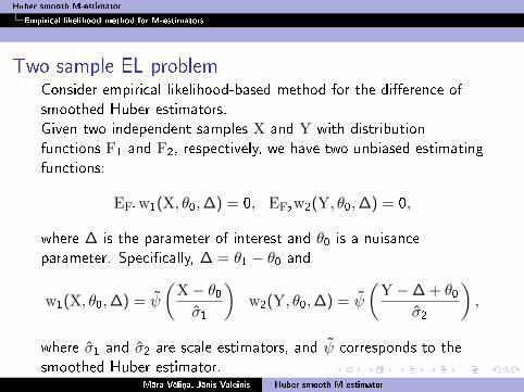
Two sample EL problemConsider empirical likelihood-based method for the difference of
smoothed Huber estimators.
Given two independent samples X and Y with distribution
functions F1 and F2, respectively, we have two unbiased estimating
functions:
EF1w1(X, θ0,∆) = 0, EF2
w2(Y, θ0,∆) = 0,
where ∆ is the parameter of interest and θ0 is a nuisance
parameter. Specifically, ∆ = θ1 − θ0 and
w1(X, θ0,∆) = ψ̃
(X− θ0σ̂1
)w2(Y, θ0,∆) = ψ̃
(Y −∆ + θ0
σ̂2
),
where σ̂1 and σ̂2 are scale estimators, and ψ̃ corresponds to the
smoothed Huber estimator.Mâra Vçliòa, Jânis Valeinis Huber smooth M-estimator

Huber smooth M-estimator
Empirical likelihood method for M-estimators
Simulation results for two sample problem
Conisder two models:
Y1 ∼ (1− ε)Gamma(α = 5;σ = 1) + εUniform[0; 50]
Y2 ∼ Gamma(α = 1;σ = 5)
Table: Coverage accuray and average confidence interval lengths basedon 1000 replicates, n1 = n2 = 50
t.int EL.hub1 EL.hub2 Boot1 Boot2
acc ave acc len acc len acc len acc len
σ = 5 0.62 3.05 0.66 2.99 0.56 2.83 0.36 2.98 0.36 2.98
σ = 6 0.69 3.56 0.73 3.51 0.65 3.34 0.38 3.46 0.38 3.47
σ = 7 0.74 4.09 0.77 4.04 0.72 3.85 0.44 3.97 0.45 3.99
σ = 8 0.78 4.62 0.81 4.56 0.76 4.39 0.48 4.49 0.48 4.50
σ = 9 0.81 5.19 0.84 5.13 0.80 4.95 0.50 5.00 0.50 5.02
Mâra Vçliòa, Jânis Valeinis Huber smooth M-estimator

Huber smooth M-estimator
Empirical likelihood method for M-estimators
Thank you for your attention!
Mâra Vçliòa, Jânis Valeinis Huber smooth M-estimator


