SS 2008, IC-SIN, No. KUMAR-SWIS-MP12 Start: 19.02.2008 Finish: 15.08.2008 Hybrid Reactions Modeling for Top-down Design Framework Lo¨ ıc Matthey X 1 X 2 + X 5 k 1 X 3 X 4 X 4 X 1 Professor: Alcherio Martinoli, Vijay Kumar Assistant: Gregory Mermoud, Spring Berman
Transcript
SS 2008, IC-SIN, No. KUMAR-SWIS-MP12Start: 19.02.2008
Finish: 15.08.2008
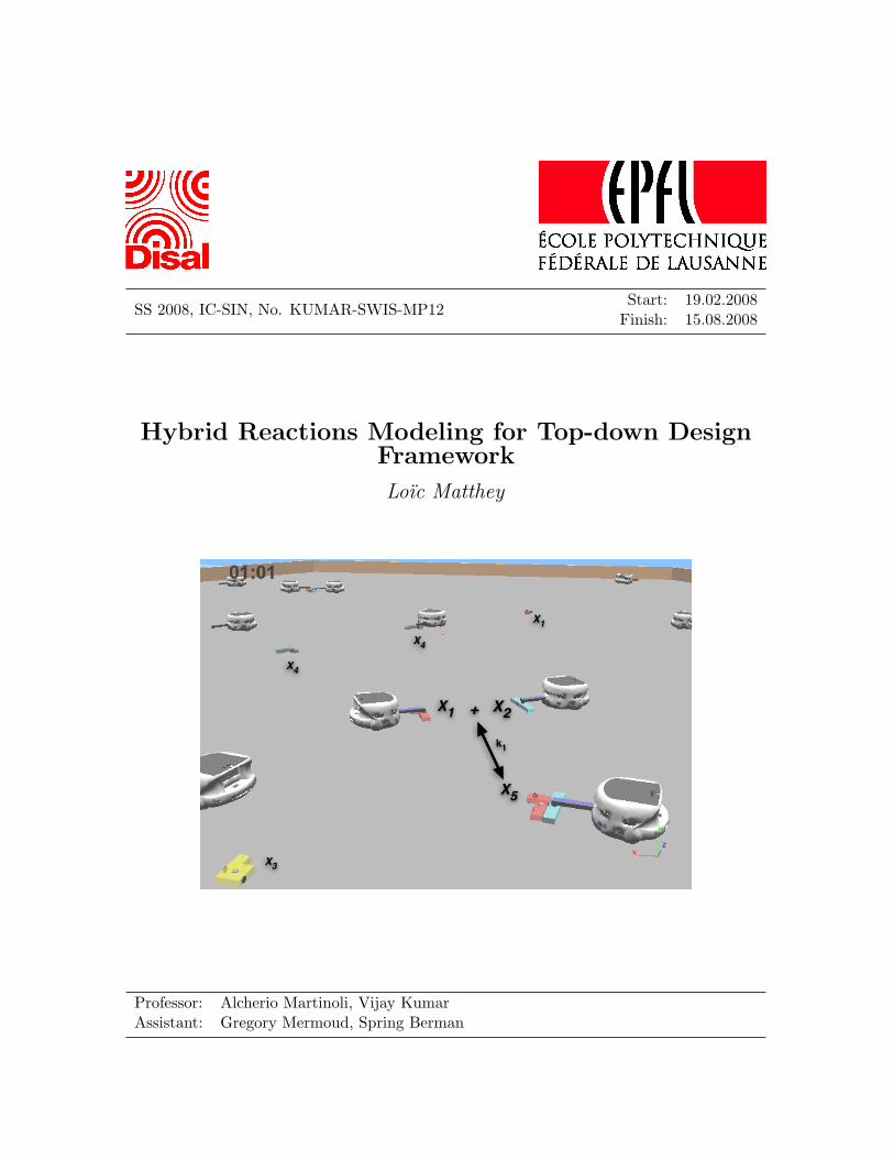
Hybrid Reactions Modeling for Top-down DesignFramework
Loıc Matthey
X1 X2+
X5
k1
X3
X4
X4
X1
Professor: Alcherio Martinoli, Vijay KumarAssistant: Gregory Mermoud, Spring Berman
This page intentionally left blank.
SS 2007-2008, No. KUMAR-SWIS-MP12 Start: 19.02.2008
Finish: 25.08.2008
Title of the project
Hybrid Reaction Modeling of the Extended Self-Assembly Problem
Author Loïc Matthey
Project description We propose a new modeling framework inspired by chemical reaction processes. Our approach consists in defining the processes and the interactions within the system in term of reactions. Such a definition can be applied to many systems, ranging from biochemical systems to swarm robotics. In particular, we aim at exploiting the toolbox developed in the context of hybrid system modeling and simulation.
The concept of extended self-assembly is the following: given a set of passive building blocks A, B, C, and D, how to obtain, with a maximal yield, the products X, Y, and Z using a set of N active transporters? What is the smallest set of reactions leading to these products? More importantly, how shall we design the building blocks and their transporters in order to fit this set of reactions? The reaction set may also involve intermediate products and be influenced by external factors. We draw inspiration from the DNA translation, and more specifically the tRNA transport molecules,which bring protein building blocks to the ribosomes. Our research may have impact on the understanding of such biological processes occuring at the nanoscale.
We envision a modeling framework that is sufficiently general to accommodate with the extended self-assembly problem, as well as the classical self-assembly problem. The validation of our models will be achieved using realistic simulation (Webots), or numerical simulations (Matlab) of various robotics systems. First, we will implement a simple example of assembly using robots as active transporters.
Tasks • Do a literature review of actual reaction rate modeling and hybrid system simulations.
• Formalize the augmented self-assembly problem. • Propose a modeling framework for the augmented self-assembly
problem. • Solve the smallest reaction set problem and the transporter
behavior problem. • Choose a test case study and model it using the framework. • Simulate the test case using Matlab and/or Webots. • Compare the results of the model and the simulation. • Depending on the results, modify and propose improvements to
better fit the data. Iterate on the last steps.
Oral presentations The date and time of the intermediate and final presentations will be specified mutually by the student, supervisor, and professor. Presentations and accompanying slides must be in English and in MS Powerpoint format. Rehearsal presentations with the project supervisor before the official talk are strongly encouraged.
Final report All of the student’s work shall be submitted on a CD (report, presentation, source code, documentation, media, etc.) as well as a hard copy of the report (English, double-sided, unbound). One copy will be required for the SWIS library (delivered to Corinne Farquharson, administrative assistant of SWIS, BC232), and additional copies may be requested by the project supervisor for his/her records. The final report must use the standard cover page and include a copy of this extended proposal just after the cover page. The report must be submitted in PDF format, and the source files (Latex recommended, MS Word accepted) should be contained in the CD-ROM, as well as the final presentation. A complete draft of the report must be submitted to the responsible supervisor at least two weeks before the final deadline. Revisions and comments will be returned in a timely fashion and will need to be incorporated into the final version of the report.
Web visibility The student’s name will be listed on the SWIS web site (under people/undergraduate) and hyperlinked to an appropriate home page if possible (either personal, or a brief page on people.epfl.ch). At the end of the project, with the help of the supervisor, a 1-page summary, a definitive project abstract, and one picture of the project will be posted (see http://swis.epfl.ch/teaching/student_projects/ for examples). It should be finalized and approved by the supervisor. Additional movies and pictures can be posted according to SWIS guidelines and after supervisor approval. This page will remain on the SWIS site under the section “past student projects” and the student’s name will be moved to the “alumni” section. The project will not be considered concluded until the dedicated web page is available on-line.
Supervision Spring Berman (UPenn), Vijay Kumar (UPenn), Grégory Mermoud
Place of work University of Pennsylvania, USA
Recommended literature DT Gillespie. Stochastic simulation of chemical kinetics. Annual Review of Physical Chemistry, 58:35–55, 2007 Eric Klavins. Programmable self-assembly. IEEE Control Systems Mag., 27:43–56, 2007 GM Whitesides and B Grzybowski. Self-assembly at all scales. Science, 295(5564):2418–2421, 2002
Signature of the Professor Prof. Alcherio Martinoli, Swarm-Intelligent Systems Group
Abstract
This report presents the work accomplished by Loıc Matthey during his Master project fromEcole Polytechnique Federale de Lausanne (EPFL). This project was a joint work between theDistributed Intelligent System and Algorithms (DISAL) Laboratory at EPFL, Switzerlandand the General Robotics, Automation, Sensing and Perception (GRASP) Laboratory atUniversity of Pennsylvania, United States of America. It took place in the Master spring-summer semester 2008.
We present a theoretical framework to design Top-down control scheme for arbitrarysystems. Being able to control a complex system using high-level instructions only is apromising and attractive paradigm. Our approach is based on the use of a Chemical ReactionNetwork model, used as a proxy to derive the control schemes. To test the application ofour method, we consider the Top-down control of a realistic multi-robots assembly platform,simulated using a 3D physics simulator, Webots.
First we present the modeling of the robotic platform using a Chemical Reaction Net-work. The free parameters are precisely fitted. We simulate the system using an ODEapproximation and an exact stochastic simulation. We find that the model can be madeto fit quantitatively to the experimental data, especially when using a stochastic simulationapproach.
Second we define an optimization and control scheme for a class of Chemical ReactionNetworks. We prove convergence results and write the optimization problem as a linearprogram of the time of convergence of the system under constraints on the equilibrium value.It allows us to design sets of reaction rates producing a specified converged behavior, inpolynomial time. This optimization provides precise controls of the system using only high-level goals.
Finally, we map the optimized model down onto the realistic physical assembly platform.We find that the system can be controlled using the optimized parameters of the model level,but that small discrepancies can have disruptive effects.
2.2 Intrinsic Complex System component. Black arrows show inter-componentcommunication, with other top-level components. Compliant Platform In-stance in bold is defined in another diagram. . . . . . . . . . . . . . . . . . . 13
2.3 Mathematical Model component. Black arrows show inter-component commu-nication. Dotted arrows show termination dependencies between components. 14
2.5 Augmented Complex System model component. Black arrows show inter-component communication. Dotted arrows show termination dependenciesbetween components. . . . . . . . . . . . . . . . . . . . . . . . . . . . . . . . . 16
2.6 Energy barrier and catalyst effect of enzymes. . . . . . . . . . . . . . . . . . . 17
4.1 Piece overview. Top connector is for the robots, side connectors are for theother pieces. . . . . . . . . . . . . . . . . . . . . . . . . . . . . . . . . . . . . . 28
4.2 Four different pieces created, with their different connecting capabilities. . . . 284.3 Assembly plans for the two final puzzles considered. All groups of connected
pieces (mid-assemblies or products) are given an unique name in a form of anumber. Arrows show the assembly steps, with their name as number. . . . . 29(a) First final puzzle plan . . . . . . . . . . . . . . . . . . . . . . . . . . . . 29(b) Second final puzzle plan . . . . . . . . . . . . . . . . . . . . . . . . . . . 29
(c) Approach between two robots and assembling of pieces. . . . . . . . . . 324.7 Physical simulation results for the robot transporter scenario, Experiment 1:
5 pieces, 4 robots and final puzzle F1 only. . . . . . . . . . . . . . . . . . . . . 34(a) Averaged populations of products over time. . . . . . . . . . . . . . . . 34(b) Histogram of the finishing times of the final puzzles F1. Red line at 400
15 pieces, 15 robots and final puzzle F1 only. . . . . . . . . . . . . . . . . . . 36(a) Averaged populations of products over time. . . . . . . . . . . . . . . . 36(b) Histogram of the finishing times of the final puzzles F1. Red line at 400
5 pieces, 5 robots and final puzzles F1 and F2. . . . . . . . . . . . . . . . . . 37(a) Averaged populations of products over time. . . . . . . . . . . . . . . . 37(b) Histogram of the finishing times of either final puzzle F1 or F2. Red line
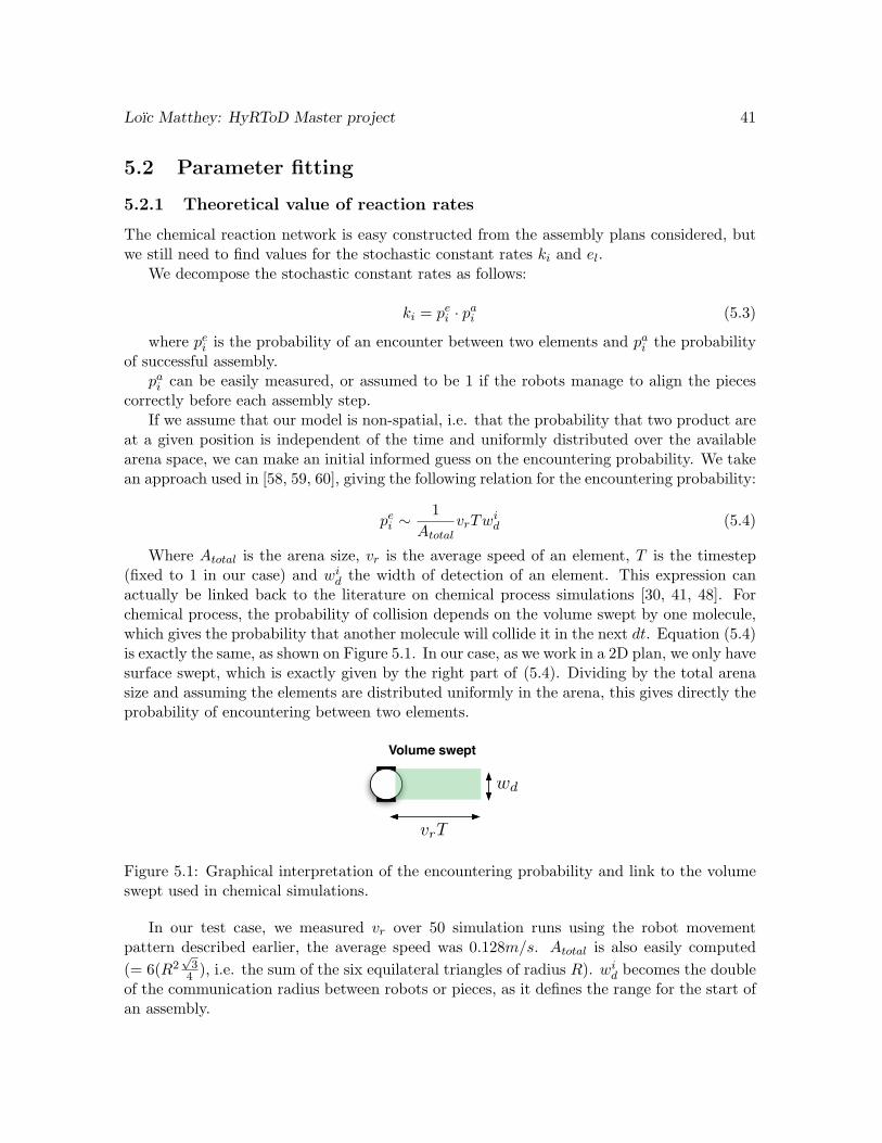
5.1 Graphical interpretation of the encountering probability and link to the volumeswept used in chemical simulations. . . . . . . . . . . . . . . . . . . . . . . . . 41
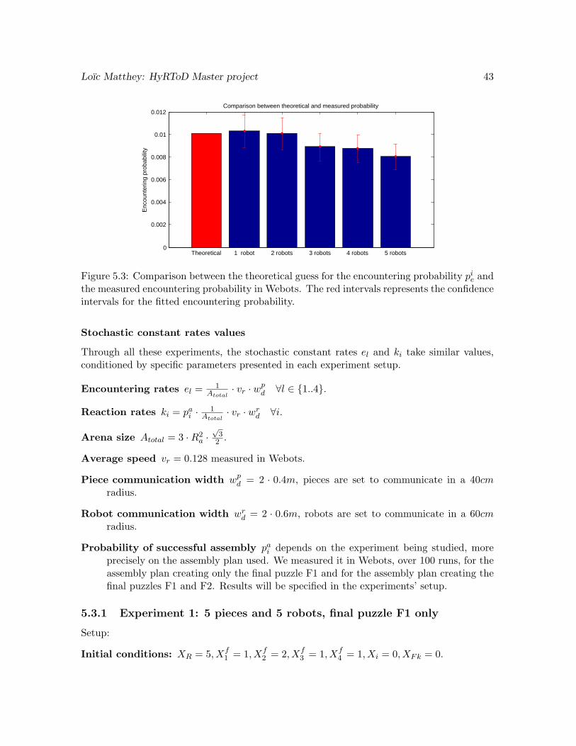
5.3 Comparison between the theoretical guess for the encountering probabilitypie and the measured encountering probability in Webots. The red intervalsrepresents the confidence intervals for the fitted encountering probability. . . 43
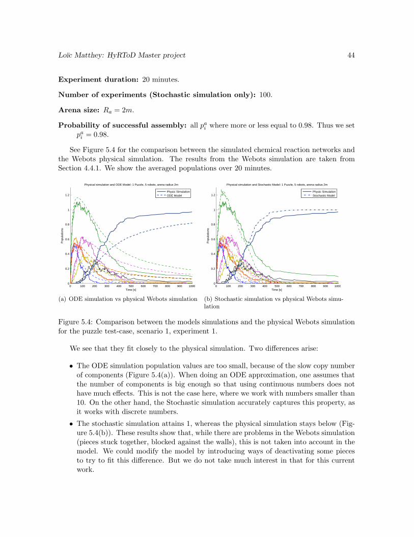
5.4 Comparison between the models simulations and the physical Webots simula-tion for the puzzle test-case, scenario 1, experiment 1. . . . . . . . . . . . . . 44(a) ODE simulation vs physical Webots simulation . . . . . . . . . . . . . . 44(b) Stochastic simulation vs physical Webots simulation . . . . . . . . . . . 44
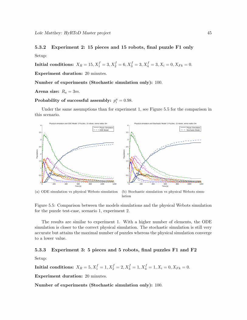
5.5 Comparison between the models simulations and the physical Webots simula-tion for the puzzle test-case, scenario 1, experiment 2. . . . . . . . . . . . . . 45(a) ODE simulation vs physical Webots simulation . . . . . . . . . . . . . . 45(b) Stochastic simulation vs physical Webots simulation . . . . . . . . . . . 45
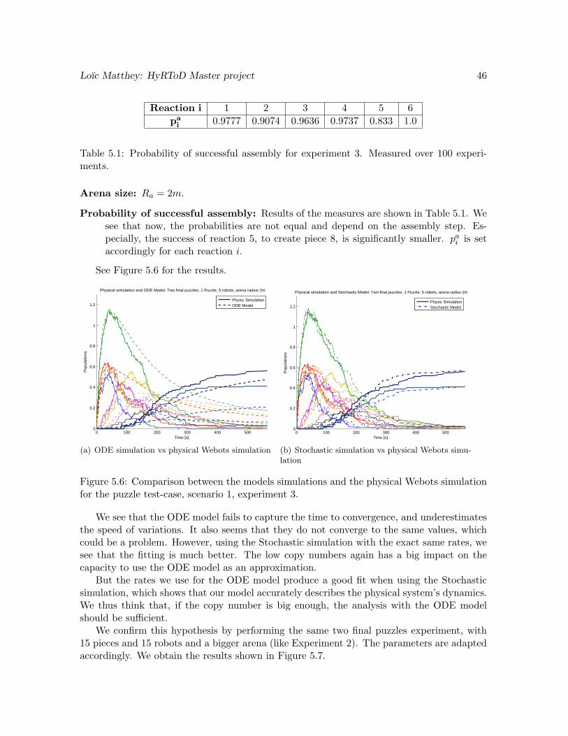
5.6 Comparison between the models simulations and the physical Webots simula-tion for the puzzle test-case, scenario 1, experiment 3. . . . . . . . . . . . . . 46(a) ODE simulation vs physical Webots simulation . . . . . . . . . . . . . . 46(b) Stochastic simulation vs physical Webots simulation . . . . . . . . . . . 46
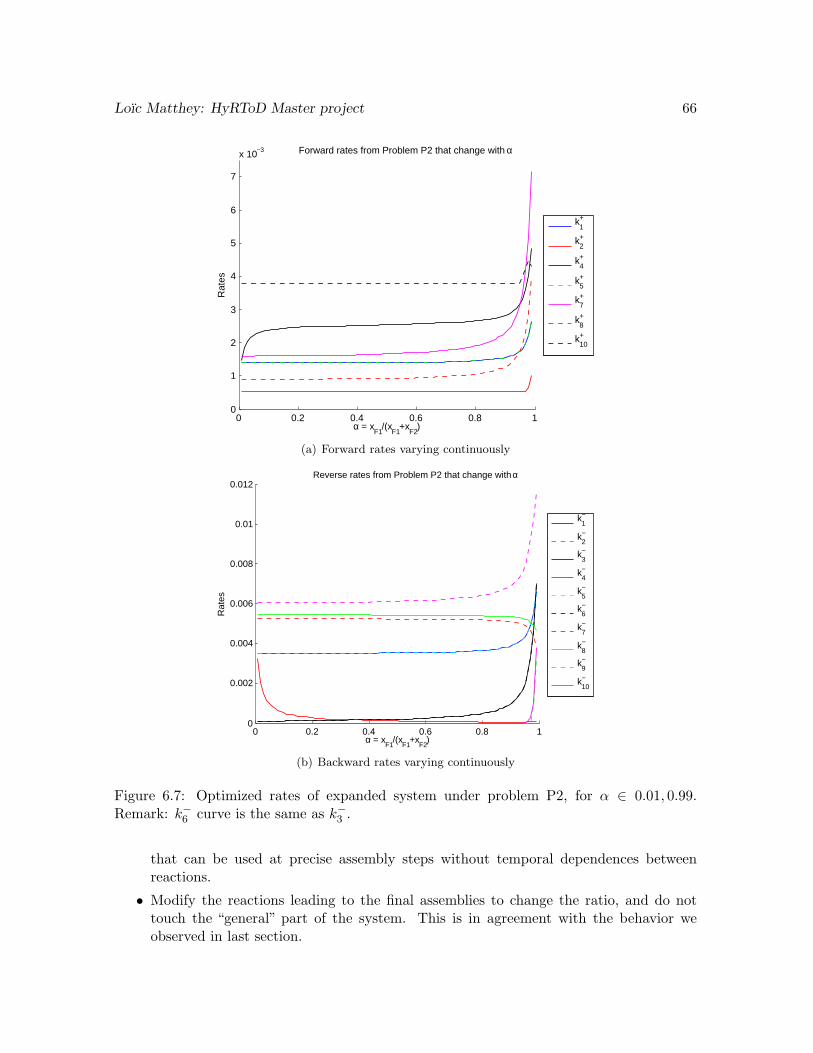
6.4 Change of reaction rates during an experiment. System adapts smoothly tothe new equilibrium. Rates are changed at the times indicated by the dottedvertical lines. First goal is 60% of F2, second is 100% of F1, third is 100% ofF2 and fourth is 50% of each. . . . . . . . . . . . . . . . . . . . . . . . . . . . 61
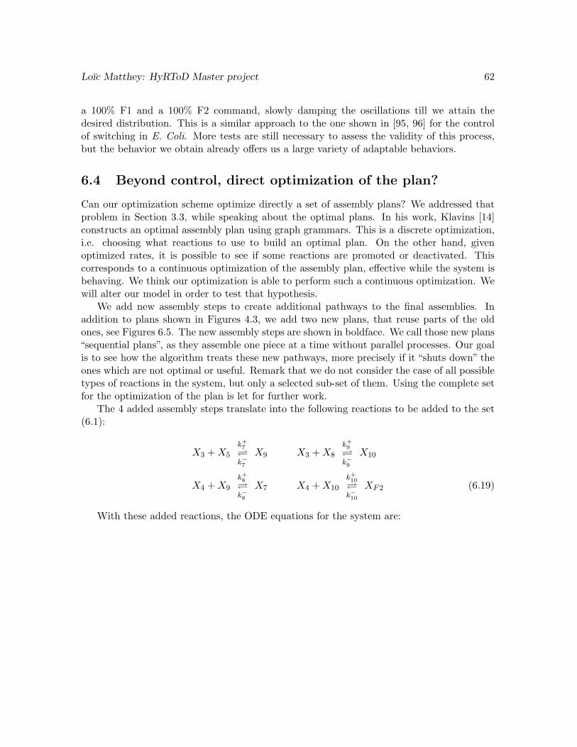
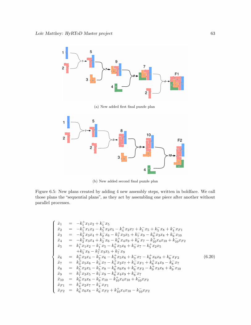
6.5 New plans created by adding 4 new assembly steps, written in boldface. Wecall those plans the “sequential plans”, as they act by assembling one pieceafter another without parallel processes. . . . . . . . . . . . . . . . . . . . . . 63(a) New added first final puzzle plan . . . . . . . . . . . . . . . . . . . . . . 63(b) New added second final puzzle plan . . . . . . . . . . . . . . . . . . . . 63
6.1 Values of optimized rates for varying α, under objective function P1 for system(6.1). Continuous rates evolve continuously with respect to α. . . . . . . . . . 57
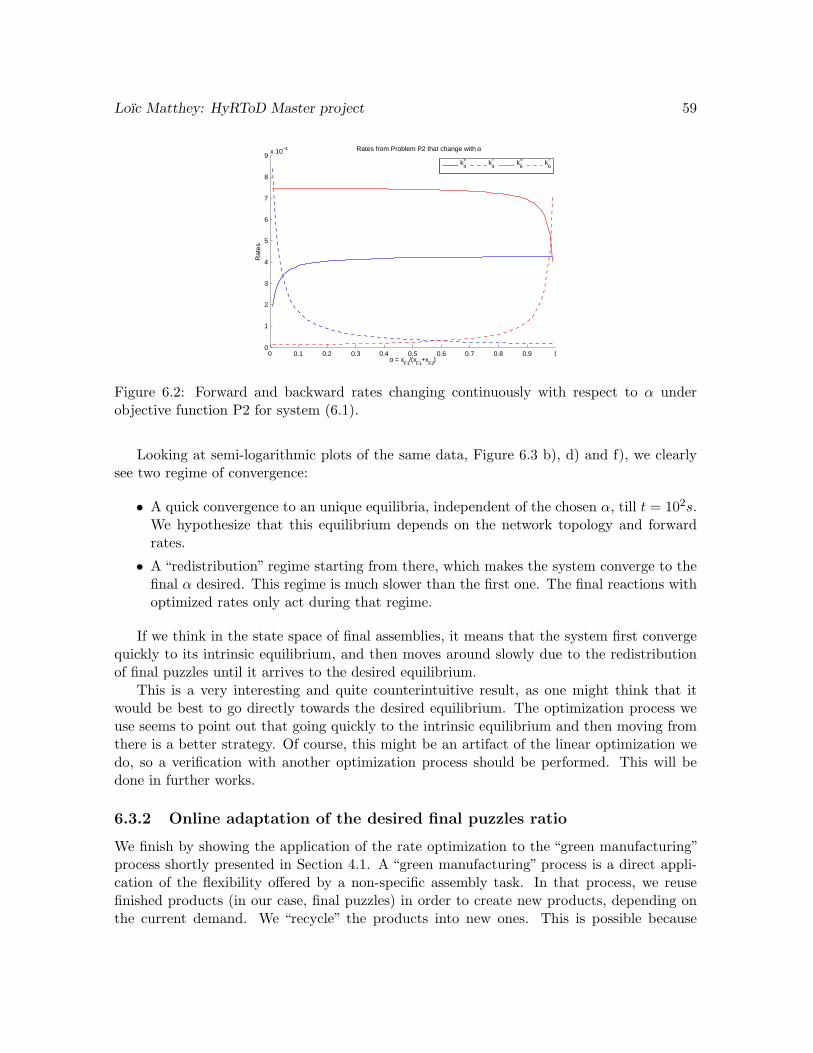
6.2 Values of optimized rates for varying α, under objective function P2 for system(6.1). Continuous rates evolve continuously with respect to α. . . . . . . . . . 58
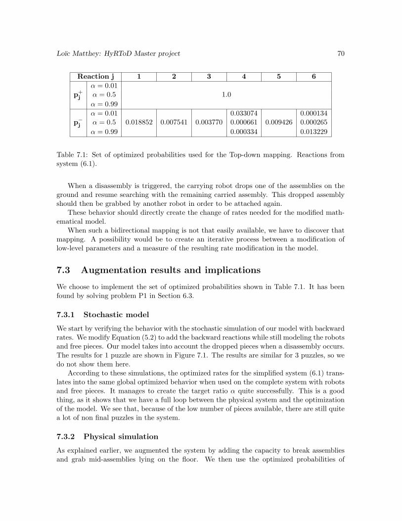
7.1 Set of optimized probabilities used for the Top-down mapping. Reactions fromsystem (6.1). . . . . . . . . . . . . . . . . . . . . . . . . . . . . . . . . . . . . 70
5.3.1 Experiment 1: 5 pieces and 5 robots, final puzzle F1 only . . . . . . . 435.3.2 Experiment 2: 15 pieces and 15 robots, final puzzle F1 only . . . . . . 455.3.3 Experiment 3: 5 pieces and 5 robots, final puzzles F1 and F2 . . . . . 45
At every scale, systems interact, collaborate and combine to create new bigger scale sys-tems. Crystals are formed by nanoscale assembly of carbon atoms, cell membranes by thearrangement of fatty acids into a lipid bilayer and human beings by the organization andcooperation of their trillions of living cells.
Yet this process, being maybe so general and vast, is still tremendously unknown.The study of self-organizing systems gives insight into the organization patterns of their
parts, and could help understanding and then modifying them.The recent field of Swarm intelligence applies the self-organizing principle to many systems
and applications, ranging from algorithmic procedures (routing of packets, meta heuristics)to team of multiple robots. This approach makes sense when the number of robots increasesto the point where a centralized or classical control methodology is not tractable anymore.Interestingly, a similar problem occurs when the scale of robots and components starts toshrink down dramatically. If the environment is intrinsically random and unknown, therobustness factor promoted by self-organizing systems becomes a key factor.
Our interest goes towards that direction. We want to study systems whose dimension isshrinking to the level where classical approaches are not applicable anymore. Furthermore,we want to model those systems, and create a framework providing a complete control flowto modify the behavior of those systems.
This might seem fairly trivial, but when the system under consideration is hard to studyby definition and not well-known, even the simplest control over them or insight in theirbehavior becomes an appreciable achievement.
Our approach is the following:
• We propose an abstract way of describing the problem under study and the actionsneeded to achieve its control. Our main claim is that it is possible to divide theproblem into two parts: an intrinsic system, on which we have no control, and anaugmented system, which encompass our additions and modifications made to modifythe behavior.
7
Loıc Matthey: HyRToD Master project 8
• We propose to use a Chemical Reaction Network mathematical framework through allthis process to model the system under study. This framework will proves itself usefulfor its flexibility and expressive power at the scale we are studying.
• We present a way to control the system via a Top-down design approach, first workingon the model and then mapping it back onto the studied system. Top-down designpeaks the interest nowadays, as being able to control a complex system using high-levelinstructions only is a promising characteristic.
• Everything is presented and verified by referring to a specific system that we createand study: a robotic platform performing a self-assembly of products.
We call it the Hybrid Reactions Modeling for Top-down Design Framework(HyRToD). “Hybrid” because we will use both ordinary differential equations approximationsand stochastic simulations to simulate the model, depending on the context.
The robotic platform is actually simulated on a computer, by using a realistic 3D physicssimulator named Webots [1]. Webots is based on ODE, an open source physics engine forsimulating 3D rigid body dynamics [2]. Such a simulator allows us to performs systematicexperiments faster than real-time and with null fabrication costs.
This might seems strange to apply a framework we claim to be thought for micrometerscale dynamics onto a high level robotic platform. We actually design the robotic platformto give it characteristics usually shown at a smaller scale, and therefore only take advantageof the robotic platform as a model system easy to measure and modify. This work focuses onthis robotic platform as a first test for our framework. Further works will consider smallerscale applications to assess our initial assumption on our framework.
1.1.1 Relations to biological processes
Even though we apply our method to a robotic implementation, a fairly high scale systemby all means, we claim that this method is applicable to many different systems, especiallythe ones governed by random dynamics.
We chose to create a robotic platform performing a self-assembly task on purpose. Havingrobots carrying the building blocks and assembling them can be thought of as an idealizationof the self-assembly process taking place into the cell, for example the protein synthesis. Ifwe allow the building blocks to move around and assemble on their own, the added robotswill behave like enzymes, promoting some reactions.
Moreover, our method, using a Chemical Reaction Network model, is very easy to applyon biological processes. This model has been extensively used in the study of biologicalsystems, and is very well understood by the community working in this field. This is anadded factor to the development of further interdisciplinary cooperations for the systems tostudy.
1.2 Outline
This report is organized as follows: Chapter 2 defines precisely our goals and the abstractproblem definition and control flow we aim to study. Chapter 3 goes over the theoretical
Loıc Matthey: HyRToD Master project 9
notions used in our work, and gives pointers to the available literature on the subject. Chap-ter 4 presents extensively the specific system we are studying, namely the physical roboticsimulation of an assembly task. Chapter 5 introduces the representation of our specific sys-tem into a Chemical Reaction Network notation, presents how we fitted the free parametersand compare the simulated results with the physical measurements. Chapter 6 is dedicatedto the optimization step applied on our mathematical model in order to control its behav-ior. Chapter 7 presents the Top-down mapping of the modified model towards the physicalsystem. Chapter 8 concludes the work and assess its validity and shortcomings.
This page intentionally left blank.
Chapter 2 Project description
2.1 Problem definition
We phrase the problem to solve as follows:
Consider an intrinsic complex system with observable dynamics and a measurableperformance metric. Let this intrinsic system attains a performance metric valueX. Introduce agents into the system with designed specific behaviors, getting anaugmented system. Can we design such behaviors so that the performance metricof the augmented system attains an new value Y , corresponding to a better orspecific behavior?
We will refer at that question as the Intrinsic System Augmentation Problem(ISAP). We believe that this formulation accurately describe an engineering methodologyfor different applications. Moreover, we argue that it is easy to represent different problemswith that framework.
The problem is decomposed in its most abstract formulation in Section 2.2. But for thisproject and thus the rest of this report, we only look at a specific instance of it. Referringto the vocabulary and decomposition of Figure 2.1, we have:
1. An intrinsic complex system representing an assembly task of a puzzle (Section 4.1).This assembly task is either a self-assembly process or an assembly process dependingon the components we put in and how we look at it. This intrinsic complex system iscreated on a simulated robotic platform (Section 4.3).
2. A mathematical model based on a Chemical Reaction Networks formulation (Chap-ter 5). We chose this formulation for its versatility and power, and because it is a wellstudied model with efficient simulations and theoretical insights.
3. An control/optimization of the model using a Convergence time optimization scheme,following the work done on Rapid Mixing Markov Chains for redistribution of a swarmof robots on multiple sites [3]. This performs a continuous optimization of our ChemicalReaction Network, namely its reaction rates. We do not address directly in this workthe discrete optimal design of this Chemical Reaction Network. See Chapter 6.
4. An augmented system presented in two different ways: either modifying the behaviorof the available agents or introducing new agents with designed behaviors. These are
11
Loıc Matthey: HyRToD Master project 12
two aspects of the same augmentation process, which have different applicability fieldsand intrinsic difficulties. See Chapter 7.
2.2 Decomposition
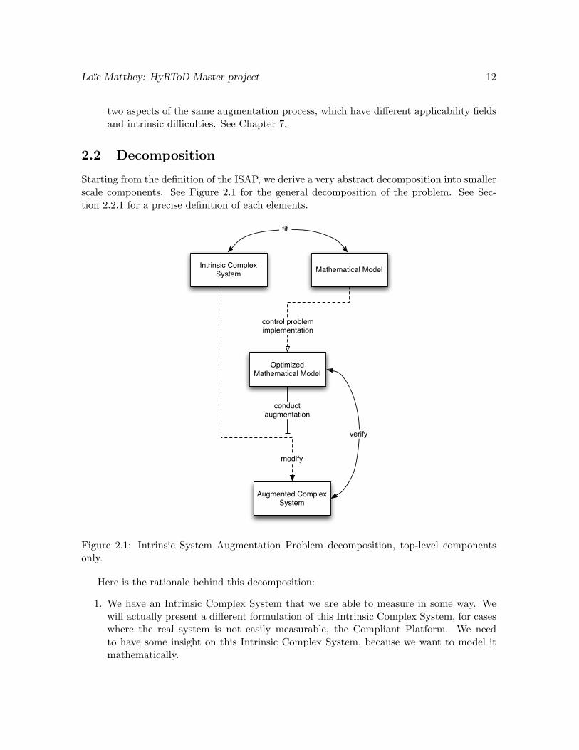
Starting from the definition of the ISAP, we derive a very abstract decomposition into smallerscale components. See Figure 2.1 for the general decomposition of the problem. See Sec-tion 2.2.1 for a precise definition of each elements.
Intrinsic Complex System Mathematical Model
Optimized Mathematical Model
Augmented Complex System
fit
control problem implementation
conduct augmentation
modify
verify
Figure 2.1: Intrinsic System Augmentation Problem decomposition, top-level componentsonly.
Here is the rationale behind this decomposition:
1. We have an Intrinsic Complex System that we are able to measure in some way. Wewill actually present a different formulation of this Intrinsic Complex System, for caseswhere the real system is not easily measurable, the Compliant Platform. We needto have some insight on this Intrinsic Complex System, because we want to model itmathematically.
Loıc Matthey: HyRToD Master project 13
2. We construct and fit a Mathematical Model of this Intrinsic Complex System. Wecan use this Mathematical Model to predict the Intrinsic Complex System, and will doseveral iterations to get the best model possible. Different modeling approaches can betaken, as well as simulations strategies for each of them.
3. We take this Mathematical Model and express it as a control problem to be solved. Thegoal can be to optimize the model for a given metric, or to change its behavior towardsa specific one. This can take a lot of forms, depending on the modeling framework usedand the level of plasticity available in the model and initial system. This new modelcan also be simulated, to verify its behavior.
4. This Augmented Mathematical Model is used to direct the augmentation of the IntrinsicComplex System into an Augmented Complex System. By “augmented”, we meanmodifying the system global behavior using one of some of the following ideas: addingnew components, modifying behaviors, modifying components. This is a Top-downapproach to complex system control. Once we know how to augment the intrinsicsystem, we have to verify that it indeed behaves like the optimized model. Hence weperform several iterations of the augmentation, so that the optimized mathematicalmodel actually captures the new Augmented Complex System.
5. We can then study the Augmented Complex System, to see what was changed for it tobehave accordingly to our goals. This could give insights for processes that are hard tostudy, especially when taking the Compliant Platform approach.
2.2.1 Project components
Intrinsic Complex System
See Figure 2.2 for the diagram. This component represent the actual system we want tostudy and modify.
There are two possibilities for this component:
Intrinsic Complex System
System state measure
Existing system Created system
Compliant Platform instanceSystem definition
Performance measure
Figure 2.2: Intrinsic Complex System component. Black arrows show inter-component com-munication, with other top-level components. Compliant Platform Instance in bold is definedin another diagram.
Loıc Matthey: HyRToD Master project 14
Existing system: In that case, we have a complex system already existing. Such applica-tions could be existing platforms for self-assembly, or an existing natural process. Weneed to be able to measure the state of this system in some way, as well as assessing itsperformance according to a desired metric. These informations are then used by theMathematical Model component or to assess the performance of the system.
Created system: If we do not have a complex system to observe, or if the actual complexsystem is not measurable, we can bypass that by creating an intrinsic complex system.For that we introduce a Compliant Platform instance. A Compliant Platform is areal or simulated platform allowing a big variety of problems reproduction. The aim isto propose a set of agents that can reproduce any given problem compatible with theirhardware capabilities. Moreover, it is possible to ensure certain properties, for examplea well-mixed property.
In this work, we use a Created system approach to reproduce a self-assembly task usinga macro-scale robotic platform. The system is created using a physical simulator, Webots.More on that is presented in Chapter 4.
Mathematical model
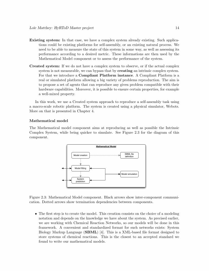
The Mathematical model component aims at reproducing as well as possible the IntrinsicComplex System, while being quicker to simulate. See Figure 2.3 for the diagram of thiscomponent.
Mathematical Model
Model creation SBML file definition
Model fitting
Model simulation
System prediction
Figure 2.3: Mathematical Model component. Black arrows show inter-component communi-cation. Dotted arrows show termination dependencies between components.
• The first step is to create the model. This creation consists on the choice of a modelingnotation and depends on the knowledge we have about the system. As precised earlier,we are working with Chemical Reaction Networks, so our models will be done in thisframework. A convenient and standardized format for such networks exists: SystemBiology Markup Language (SBML) [4]. This is a XML-based file format designed tostore systems of chemical reactions. This is the closest to an accepted standard wefound to write our mathematical models.
Loıc Matthey: HyRToD Master project 15
• The model has to be fitted in some way to the Intrinsic Complex System. If we areusing an existing complex system, then this is a quite complex problem, especially ifwe do not have precise insight in the behavior of the system. We can use methods likeBayesian Inference or MCMC (Markov Chain Monte Carlo) to fit the model on theexperimental data. If we are using the Compliant Platform, than we assume that wecan measure much more precisely the processes taken place, and this model fitting ismore straightforward.
• We also need a simulation framework for the mathematical model. For Chemical Reac-tion Networks, a lot of literature is available on that. As we will present in Section 3.2.2,we use either a direct Stochastic simulation or a simple ordinary differential equationsolver.
Optimized Mathematical model
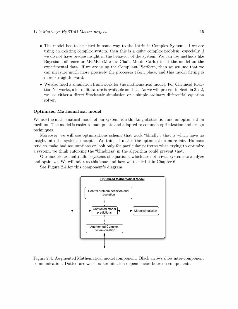
We use the mathematical model of our system as a thinking abstraction and an optimizationmedium. The model is easier to manipulate and adapted to common optimization and designtechniques.
Moreover, we will use optimizations scheme that work “blindly”, that is which have noinsight into the system concepts. We think it makes the optimization more fair. Humanstend to make bad assumptions or look only for particular patterns when trying to optimizea system, we think enforcing the “blindness” in the algorithm could prevent that.
Our models are multi-affine systems of equations, which are not trivial systems to analyzeand optimize. We will address this issue and how we tackled it in Chapter 6.
See Figure 2.4 for this component’s diagram.
Optimized Mathematical Model
Control problem definition and resolution
Model simulationControlled model predictions
Augmented Complex System creation
Figure 2.4: Augmented Mathematical model component. Black arrows show inter-componentcommunication. Dotted arrows show termination dependencies between components.
Loıc Matthey: HyRToD Master project 16
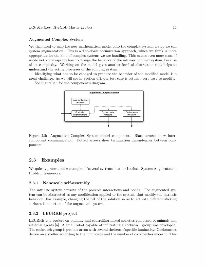
Augmented Complex System
We then need to map the new mathematical model onto the complex system, a step we callsystem augmentation. This is a Top-down optimization approach, which we think is moreappropriate for the kind of complex systems we are handling. This makes even more sense ifwe do not know a-priori how to change the behavior of the intrinsic complex system, becauseof its complexity. Working on the model gives another level of abstraction that helps tounderstand the acting processes of the complex system.
Identifying what has to be changed to produce the behavior of the modified model is agreat challenge. As we will see in Section 6.3, our test case is actually very easy to modify.
See Figure 2.5 for the component’s diagram.
Augmented Complex System
Augmentations definition
Controlled augmentations
System state measure
Performance measure
Figure 2.5: Augmented Complex System model component. Black arrows show inter-component communication. Dotted arrows show termination dependencies between com-ponents.
2.3 Examples
We quickly present some examples of several systems into our Intrinsic System AugmentationProblem framework.
2.3.1 Nanoscale self-assembly
The intrinsic system consists of the possible interactions and bonds. The augmented sys-tem can be abstracted as any modification applied to the system, that modify the intrinsicbehavior. For example, changing the pH of the solution so as to activate different stickingsurfaces is an action of the augmented system.
2.3.2 LEURRE project
LEURRE is a project on building and controlling mixed societies composed of animals andartificial agents [5]. A small robot capable of infiltrating a cockroach group was developed.The cockroach group is put in a arena with several shelters of specific luminosity. Cockroachesdecide on a shelter according to the luminosity and the number of cockroaches under it. This
Loıc Matthey: HyRToD Master project 17
is a self-organized decision process. The robot were able to infiltrate this group and to directthe global decision of the group. The infiltrated robots made the cockroaches go under alight shelter, a configuration which was never attained with the cockroaches group only.
Intrinsic system: the cockroach group. The metric is the probability of the different shel-ters as final decision.
Augmented system: the cockroaches and the robots. The robots choose a different shelter,this action in turn modify the final probability of the shelters.
2.3.3 Enzymes
In living cells, chemical reactions takes place whenever compounds needs to be transformedor created. For chemical processes needing energy to occur, one usually see a energy barriermechanism, see Figure 2.6. Before a reaction can occur, activation energy has to be provided,to pass the barrier. When adding enzymes to the system, they catalyze the reaction andproduce a virtual decrease of the needed activation energy. Enzyme can act by improvingfitting of compounds, stabilizing transitions or modifying orientations.
Figure 2.6: Energy barrier and catalyst effect of enzymes.
Intrinsic system: The original chemical reaction, with specific activation energy and rates.
Augmented system: The catalyzed chemical reaction with the introduction of the enzyme.The enzyme performs an action (binding with change of conformation) that reducesthe activation energy and increase the rate of the chemical reaction.
2.3.4 RNA translation into proteins
In living cells, DNA contains the blueprints for every functional proteins. In the cell nucleus,it is first transcripted into RNA, which is translocated to the cytoplasm to be translated
Loıc Matthey: HyRToD Master project 18
into proteins. The RNA strands contains the building plan, and special proteins, calledribosomes, attach on it in order to “read” it and assemble amino acids (the basic buildingblocks of proteins) according to this plan. These amino acids are created as a linear chain (firststructure), that fold onto itself according to low-energy bounds, acquiring a tridimensionalstructure called a conformation (second and tertiary structure). A protein is a sequence ofamino acids in a specific conformation that allows its functional activity.
Intrinsic system: Ribosomes assemble amino acids according to the RNA code. The ob-tained first structure protein then folds itself into a specific conformation.
Augmented system: Chaperone protein helps the folding of the protein, possibly modify-ing the obtained conformation or allowing the initial one under different environmentconditions (heat-shock response).
Chapter 3 Field overview
3.1 Self-assembly engineering
This work has been triggered by an interest in the simulation and modeling of self-assemblingprocesses. Such process can take many forms, from nano-scale assembly [6, 7, 8] to controlof biomolecules [9, 10, 11, 12] up to modular robotics [13, 14]. This field is gaining more andmore attention nowadays [15].
3.1.1 Microscale assembly
Of all these applications, microscale assembly is the one which gathered the most interest inthe last few years and which promises the most interesting future applications [15, 16].
While pursuing the race towards even more miniaturization, we are facing new problemsthat current technologies and methodologies have trouble solving. The lithography process,used to create all the microchip used now, is getting to its limit [15]. New approaches becomenecessary.
The current technology for microscale assembly is still in its infancy [15]. The current stateof research aims at attaching pieces together at specific positions. This either creates biggerscale components, or combines functional devices created via traditional methods. Severalmethods are currently under study [17, 18, 19, 6], ranging from attaching mechanisms toprototyping methods.
However, such mechanisms are still far from the kind of control we have on the higherscale assembly, and all those processes have a very low production yield. But microscaleassembly opens the door to a whole new world of possibilities for integration, system repairsand even active drugs.
An interesting distinction for self-assembly, made by Whitesides [15], is the differencebetween static and dynamic self-assembly. In static self-assembly, the components onceformed stay stable and stop dissipating energy. In dynamic self-assembly, energy is dissipatedand should be produced or given in some way. A living cell is a typical example of dynamicself-assembly.
Our works aims at studying such dynamical self-assembly, yet at a scale closer to biology(millimeter scale) than microscale scale.
19
Loıc Matthey: HyRToD Master project 20
3.1.2 Modular robotics
As we aim at using robots as a platform for our work, our works is similar to studies donein modular robotics.
Modular robotics encompass any robotic system that can deliberately change its ownshape, in order to adapt to new circumstances, perform new tasks or recover from dam-age [13][20].
A work close to our approach is the one done by E. Klavins on programable self-assembly [14,21, 22, 23]. His work revolves around the assembly of triangular robots, moving around ran-domly on an air table and capable of assembling themselves according to a given plan.
The plan itself is constructed with a grammar approach, working with graph grammars.A graph grammar is a set of rules transforming a graph when applied on it. The assembly isrepresented as a sequence of application of rules, transforming the initial set of products intoa final graph representing the final assembly. Klavins showed methods to construct graphgrammars automatically for a given final assembly [23].
These grammars are then used with the robots to converge to a final shape constructedonly by self-assembly.
In the first versions of this approach, the particularities of the assembling process, such asgeometric difficulties and disassemblies due to shocks, were not taken into account. Klavinsaccounted for them by measuring the kinetic rate constants of assemblies, and then tryingto modify the plan accordingly [14].
Our approach on the other hand, directly takes into account those reaction rates, makingthem central and essential to our approach. We think that finding an “optimal” theoreticalplan is useless when this plan could become “sub-optimal” under the constraints of the reac-tions rates. These rates directly show the physical characteristics of the system to assemble,they are not easily modified.
This is also why we will use an approach using Chemical Reaction Networks for our plansand models: they are build to take into account the intrinsic reaction rates of the systems.
Furthermore, we study a system of heterogenous parts, adding a specificity and complexityrequiring different analysis and techniques.
3.2 Chemical reaction networks
3.2.1 Theory
Through this project, we use a Chemical Reaction Networks notation and framework asmathematical model. This has been introduced in the context of chemical processes in1979 [24] and has been very researched since then.
This level of representation is at the same time very general, offering representation of verydifferent processes, and also quite precise and detailed, allowing to construct full dynamicsimulations of the system behavior on a computer. This introduction to chemical reactionsis adapted from the textbook of J.Wilkinson [25].
Where r is the number of reactants and p the number of products. Ri is the ith reactantmolecule and Pj the jth product molecule. mi is the number of molecules of Ri consumed ina single reaction step, and nj the number of molecules of Pj produced. The coefficients mi
and nj are known as stoichiometries.A chemical reaction networks consists of several of these reactions, possibly sharing reac-
tants and/or products. If a reaction can occur in both directions, meaning that the productsin the right part can be transformed in the reactants of the left part with the same stoi-chiometries, we call this reaction reversible. A reversible reaction is written as follows (for asimple dimerisation example), see Eq. (3.2).
2P P2 (3.2)
Such networks represent the possible actions of the systems and the relations betweenthe elements. But it does not represent the dynamics directly. To add this information, wehave to make an assumption on the type of dynamics governing the system.
In chemical system, a classical governing dynamic is a mass-action stochastic kinetics [26].In this formulation, we associate to each reaction Ri a stochastic rate constant, ci, and anassociated rate law (or propensity function) hi(x, ci), where x = (x1, x2, . . . , xu) is the currentstate of the system. The form of hi(x, ci) (and the interpretation of the rate constant ci), isdetermined by the order of reaction Ri. In every cases, the propensity function has the sameinterpretation: conditional on the state being x at time t, we then have that the probabilitythat an Ri reaction will occur in the time interval (t, t+ dt] is given by hi(x, ci)dt [25].
The classical orders of reactions and their propensity functions are as follows:
Zeroth-order Ri : ∅ ci−→ X
This represents a constant rate of production of a chemical specie.hi(x, ci) = ci.
First-order Ri : Xjci−→?
This is the spontaneous transformation of a reactant into new products.hi(x, ci) = cixj , as there are xj molecules of Xj .
Second-order Ri : Xj +Xkci−→?
This represents a reaction between a pair of reactants.hi(x, ci) = cixjxk, for all combined pairs of molecules Xj , Xk. Special case if Xj = Xk:hi(x, ci) = ci
xj(xj−1)2 .
Higher orders Those can be transformed back into second-order reactions, as we make theassumption that a third-order reaction is impossible and actually corresponds to thecombined effect of two second-order reactions.
This allows then to simulate exactly the modeled process assuming we know all the rateconstants and rate laws.
Nowadays, simulation of multiscale systems have become the new interest. A multiscalesystem is characterized either on the timescale aspect or the copy number of reactants [27].
Loıc Matthey: HyRToD Master project 22
1. For the timescale aspect, the different scales arise when some reactions are much fasterthan others. They then quickly reach a stable state, and the global dynamics of thesystem is driven by the slow reactions.
2. For the copy number of reactants, the difference comes from the relative size of thepopulations. Species with a small population are best viewed as discrete stochasticprocesses, while the large populations should follow a deterministic model.
Such systems, called stiff systems, present new problem to commonly used simulations al-gorithm. They also are of increasing interest in system biology, as a lot of real biologicalprocess operates on multiple scales.
3.2.2 Simulation algorithms
Several ways of simulating chemical reaction networks are available.
Ordinary differential equation
The simplest one, and the most used by chemists because of thermodynamical limits andnumber of molecules involved, is to use the associated ordinary differential equation (ODE).One can represent the populations (or concentration, given a finite volume V ) of all products,and treat the reactions as outflow and inflow acting on those populations. If we take thesimple dimerisation system (3.2), assuming a forward rate k+ and a backward rate k−, weobtain:
P = −k+P (P − 1)2
+ k−P2 (3.3)
P2 = k+P (P − 1)2
− k−P2 (3.4)
Such a transformation is automatic for any chemical reaction network with reactions upto second-order. We can then simulate it using classical numerical integration methods. Notethat ODE use continuous number for the populations. Therefore, this approximation canbe wrong when the copy number of elements (the number of elements) is small. In classicalchemical contexts, the copy numbers are very high (near Avogadro’s number), so this is notan issue.
Gillespie Stochastic simulation algorithm
It has been shown by Gillespie [28, 29, 30, 31, 32], that it is possible to perform an exactsimulation of a chemical reaction networks. The algorithm is referred to as the Direct Methodor Gillespie Stochastic Simulation Algorithm (SSA). It takes advantage of the fact that thetime-evolution of a reaction network can be regarded as a stochastic process, and, becausethe propensity functions depends only on the current state, the system is a continuous timeMarkov process with a discrete state space. The time to the next reaction follows a expo-nential distribution Exp(h0(x, c)), with h0(x, c) =
∑vi=1 hi(x, ci) and v reactions. The type
Loıc Matthey: HyRToD Master project 23
of reaction is independent of that time, and is given by the probability hi(x, ci)/h0(x, c). Wecan then simulate the system for each reaction events, up to a desired finishing time.
This algorithm, however, is highly inefficient when the number of products and reactantsincreases. Several optimization have thus been proposed to cope for that limitation.
Tau-leaping
Gillespie first proposed optimization, the tau-leaping optimization [33], aims at make thesystem evolve for a time τ where a certain amount of reactions fire instead of simulatingevery reaction. It is based on the assumption that the propensity functions aj(x), governingthe rates of firing of the reactions, stays nearly constant for a certain time τ . It is then possibleto approximate the number of reaction firings during that time τ by a Poisson process of rateaj(x)τ .
Automatic ways of finding τ also have been proposed [34], as well as different variations ofthe tau-leaping: Implicit tau-leaping (performs better for stiff systems) [35], Trapezoidal tau-leaping (more efficient than explicit tau-leaping), and the latest explicit-implicit tau-leaping(combination of the two regimes) [36].
The principle of simulating several reactions events at the same time is also used inanother very known algorithm, called the Gibson & Bruck Next Reaction algorithm [37].
Multiscale systems
To simulate multiscale systems with different timescales, Gillespie proposed the Slow ScaleStochastic Simulation Algorithm (ssSSA) [38, 36, 39, 40]. This algorithm uses a quasy steady-state approximation for the fast reactions of the system. The algorithm explicitly simulatesonly the slow reactions, the fast ones take values governed by steady-states assumptions ofconvergence. Gillespie defines for that virtual fast processes, that are not touched by theslow reactions. These virtual fast processes can then gives the new populations for the fastspecies, without simulating them explicitly.
Other ways of simulating multiscale systems have been proposed [41]. One of themsuggests to simulate the fast reactions using a deterministic approximation [42, 43, 44]. Thegoal is to replace the stochastic processes of the fast reactions with big population by an ODE.In this manner, fast simulation of the fast reactions can be attained, while keeping stochasticsimulations for the slow reactions. This Stochastic-deterministic approximation may still posesome convergence problems, as no real proofs of convergence toward the stochastic averagesof the initial fully stochastic system have been provided.
To complete this overview, there are also algorithm simulating the reactions in a spatially-dependent context, by using diffusion methods [45, 46, 47, 48].
Several toolkits implementing those simulations algorithm are available [49, 50, 51].
3.3 Considerations on the assembly plan
Continuing on the discussion with Klavins’ approach to self-assembly, we discuss the problemof the assembly plan and its relation to the reaction rates.
Loıc Matthey: HyRToD Master project 24
The complete problem of constructing a final assembly from initial parts can be dividedinto two parts: a discrete and a continuous one.
1. The discrete part consists of the assembly plan itself. It represents a finite and discreteset of rules to construct the final target.
2. The continuous part is the rate of evolution of the assembly, driven by the assemblyplan but subject to continuous reaction rates. Those rates can take continuous valueswhich will affect the final outcome of the assembly.
We argue that, taken to the limit, the problem is actually completely continuous. Thereaction rates, when pushed toward 0, will deactivate a part of the assembly plan automati-cally.
We wish then to study the optimization of these continuous reaction rates, as we thinkthey might give more insight on the relations between parts of the plan and as they encompassthe same power as the discrete part.
In order to go in that direction completely, one would need to consider the “full assemblyplan”. Such a plan would consists of every possible assembly steps towards the creation ofa final assembly. Indeed, it would become quite big quickly, but pruning is possible, mainlybecause we assume that we have heterogenous pieces that have highly specific assemblingsites. Such a plan is easily obtained using any enumeration method, for example Polyaenumeration [52].
But in this work, we only consider a subset of this “full assembly plan”. We assume thatwe are given a part of this plan, which already creates the final assembly. We then studyonly the effect of the reactions rates on this plan, and see what parts of it an optimizationtechnique will push forward or cut down. This is an assumed simplification for the currentwork.
Chapter 4 Puzzle test-case implementa-tion
We apply our framework and methodology on a specific problem: A puzzle assembly task.The goal is to assemble several heterogenous pieces together to create a specific final shape.This is done using a robotic platform, simulated using a realistic physics simulator: We-bots [1].
This allows us to get a measurable system which could be transformed into a real platformpretty easily.
4.1 Definition of the puzzle test-case
We define the puzzle test-case as follows:
• Let a puzzle of square shape, with area 25, be constructed out of 5 pieces of area 5 eachwith different given shapes.
• Let the final assembly shapes Sk of this puzzle be know.
• Let the set of assembly plans Pk leading to the final shapes Sk be known.
• Let the puzzle pieces assemble by bi-directional connections. One connection is enoughfor two pieces to be attached. These connection and their positions on the differentpieces are known.
• Pieces can be assembled and disassembled.
• Piece can lie around or move randomly. We study those two possibilities, but weconcentrate on the first one.
• Consider an arena of sufficiently large size so that small scale interactions dynamicscan be ignored.
• Fill this arena with ni initial pieces of each shape i. Let these ni number be the exactnumbers needed to construct N final assemblies.
• Consider M robots, able to pick up pieces and to make them assemble and disassemble.
• Allow a recognition by the robots and by the pieces of the shapes and connection pointswhen an encounter occur.
• Then:How can you manipulate those initial pieces so that after a time Tf , the number of
25
Loıc Matthey: HyRToD Master project 26
assembled puzzles XSkcorresponds to desired values?
We introduced here the goal of this whole test case: to control the output of the systemin term of assembled puzzles.
This can also be applied on the fly, to control what the system should produce. We wanthere to take advantage of the modularity of the platform, as our robots can produce anydesired assembly.
An application of that flexibility can be what we call a green manufacturing process. Wemean by that the automatic recycling of finished puzzles S1 to create new puzzles S2, onlyby telling the robots what we want as final assembly. This will be studied in Chapter 6.
4.2 Scale and complexity considerations
We have a lot of different possibilities for the robot behaviors. We chose to consider differentdirections depending on the available information and capabilities of the robots. If we wantto produce something really scalable, then using robots as simple as possible is interesting.But on the other hand, this would most likely affect the performances. So we will try tomeasure this with respect to several considerations.
Assembly plan known Local plans onlyLocal information Current study Future work
Global information Market-based, Assembly line Market-based
Table 4.1: Robot behavior depending on available informations.
The first distinctions we make are shown in Table 4.1. The most important criteria isthe availability of information about the robots and pieces positions and states. If we havea Global information state, then the problem reduces to a classical assembly at the macro-level. With multiple robots, this could be solved using Market-based strategies, which do notinterest us here. So we only consider having Local information about the pieces and robotspositions.
The next distinction is the availability of the full assembly plan. Knowing the full assemblyallows to optimize a-priori a plan and to stick to it when building the puzzle. But this needssome computing capabilities and communications between pieces and robots. A more crudepossibility is forbidding this full knowledge, and having to recreate the global plan only fromlocal connections possibilities.
We are currently studying the Local info / Assembly plan case. The Local info / Localplan case is very interesting but will be done in further works.
Furthermore, we have the following choice to make: should the pieces be disassembled ornot? As we will develop during the project, this depends on the possibility of bad assembliesand on the flexibility of creation needed. Indeed, if we want to apply our system to the greenassembly process, we have to be able to destroy final products into simpler ones.
This is in accordance with biology, which tends to reuse products and compounds fordifferent purposes. This allows a flexibility and adaptation necessary when we do not know
Loıc Matthey: HyRToD Master project 27
the goal a priori.A quick precision should be done on the moving capabilities of pieces. We concentrate here
on the task of assembling immobile pieces. In this case, the robots behaves like transporters.But, seen more abstractly, this is the same as having moving pieces on their own. Wealso study the case of pieces moving around randomly. This simulates more closely a self-assembly task, driven only by geometric constraints for the assembly. An interesting scenariois to add robots to the system with moving pieces. In this setup, the added robots behaveslike enzymes: they modify the system by acting on it. This creates three different scenario:the robot-transporter, the self-assembling pieces and the mixed assembly.
In all this section, we only consider forward assemblies of pieces, that is, we never disas-semble things. This will be explored further on, in the Augmentation step, Chapter 7.
4.3 Webots implementation
We chose to develop our puzzle test case using the realistic physic simulator Webots [1]. Thisallows us to simulate robots and assembly process, while still being affected by noise andgeometric properties. We could have developed a simpler simulator, for example a point-basedsimulator for an assembly process, but we think that the added physical reality of Webotsmakes it easier to understand how real-world problems could behave in our framework.
Webots offers directly a capability to assemble our puzzle pieces: connectors. Theseconnectors behaves like active electromagnets, that can be turned on and off. The goal is tomimic the assembly process of molecular compounds, tied by low-energy bounds.
The first implementation of the controllers for the robot transporters scenario on Webotshas been created by Spring Berman for her project in the course MEAM620 by V. Kumarat the University of Pennsylvania. Loıc Matthey created the Webots worlds and subsequentlymodified the controllers code to improve scalability, add the support for arbitrary assemblyplans, change the movement patterns and create the self-assembly and mixed-assembly sce-narios.
4.3.1 Pieces
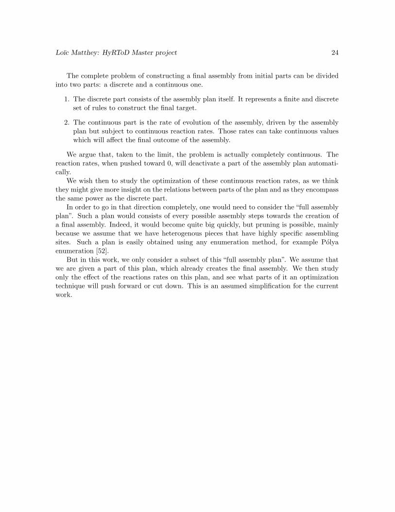
A piece consists of a solid body, several small feet and several connectors. There is only onetop connector for the robots to carry the piece around. There are several side connectors,to connect to other pieces, their number depend on the piece type. See Figure 4.1 for anexample of such a piece.
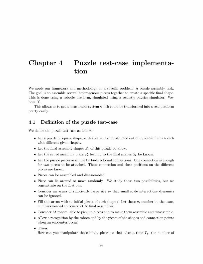
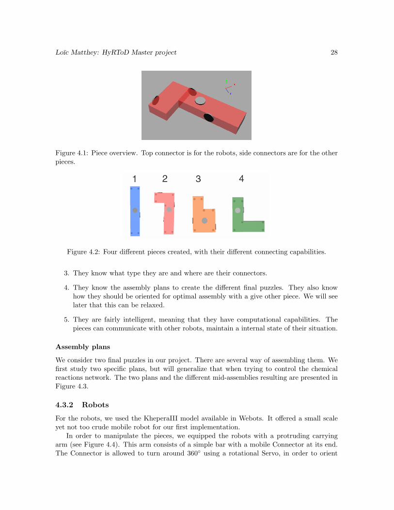
We created a set of four different pieces, each with different shapes and different connect-ing capabilities. See Figure 4.2 for the different pieces.
These pieces are endowed with several other capabilities:
1. They have a radio emitter/receiver to communicate with robots or other pieces. Thecommunication range is set to 40cm for the pieces.
2. They can activate or deactivate their connectors at will.
Loıc Matthey: HyRToD Master project 28
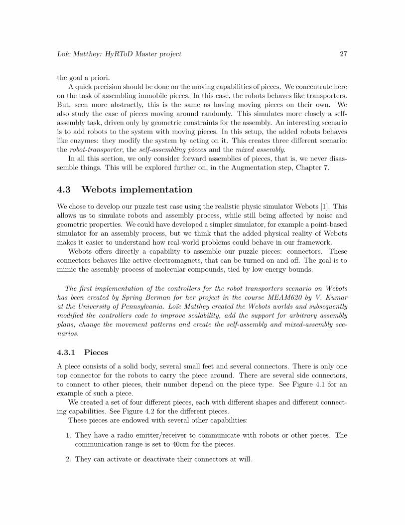
Figure 4.1: Piece overview. Top connector is for the robots, side connectors are for the otherpieces.
Figure 4.2: Four different pieces created, with their different connecting capabilities.
3. They know what type they are and where are their connectors.
4. They know the assembly plans to create the different final puzzles. They also knowhow they should be oriented for optimal assembly with a give other piece. We will seelater that this can be relaxed.
5. They are fairly intelligent, meaning that they have computational capabilities. Thepieces can communicate with other robots, maintain a internal state of their situation.
Assembly plans
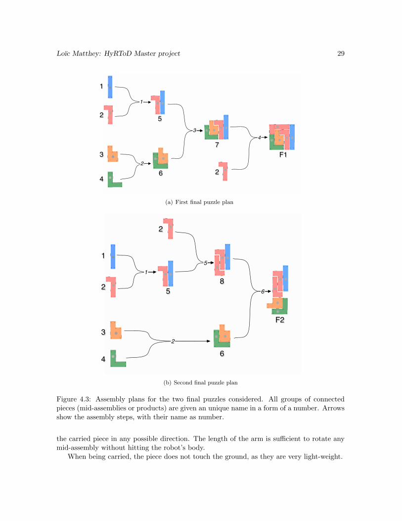
We consider two final puzzles in our project. There are several way of assembling them. Wefirst study two specific plans, but will generalize that when trying to control the chemicalreactions network. The two plans and the different mid-assemblies resulting are presented inFigure 4.3.
4.3.2 Robots
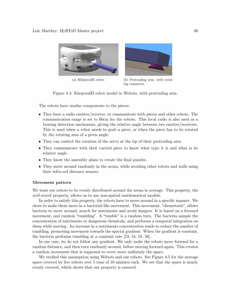
For the robots, we used the KheperaIII model available in Webots. It offered a small scaleyet not too crude mobile robot for our first implementation.
In order to manipulate the pieces, we equipped the robots with a protruding carryingarm (see Figure 4.4). This arm consists of a simple bar with a mobile Connector at its end.The Connector is allowed to turn around 360◦ using a rotational Servo, in order to orient
Loıc Matthey: HyRToD Master project 29
1
2
3
4
5
6
7
2
F1
1
2
34
(a) First final puzzle plan
1
2
3
4
5
6
8
F2
2
2
15
6
(b) Second final puzzle plan
Figure 4.3: Assembly plans for the two final puzzles considered. All groups of connectedpieces (mid-assemblies or products) are given an unique name in a form of a number. Arrowsshow the assembly steps, with their name as number.
the carried piece in any possible direction. The length of the arm is sufficient to rotate anymid-assembly without hitting the robot’s body.
When being carried, the piece does not touch the ground, as they are very light-weight.
Loıc Matthey: HyRToD Master project 30
(a) (b) (c) (a) KheperaIII robot.
(a) (b) (c) (b) Protruding arm, with rotat-ing connector.
Figure 4.4: KheperaIII robot model in Webots, with protruding arm.
The robots have similar components to the pieces:
• They have a radio emitter/receiver, to communicate with pieces and other robots. Thecommunication range is set to 60cm for the robots. This local radio is also used as abearing detection mechanism, giving the relative angle between two emitter/receivers.This is used when a robot needs to grab a piece, or when the piece has to be rotatedby the rotating arm of a given angle.
• They can control the rotation of the servo at the tip of their protruding arm.
• They communicate with their carried piece to know what type it is and what is itsrelative angle.
• They know the assembly plans to create the final puzzles.
• They move around randomly in the arena, while avoiding other robots and walls usingtheir infra-red distance sensors.
Movement pattern
We want our robots to be evenly distributed around the arena in average. This property, thewell-mixed property, allows us to use non-spatial mathematical models.
In order to satisfy this property, the robots have to move around in a specific manner. Wechose to make them move in a bacterial-like movement. This movement, “chemotaxis”, allowsbacteria to move around, search for nutriments and avoid dangers. It is based on a forwardmovement, and random “tumbling”. A “tumble” is a random turn. The bacteria sample theconcentration of nutriments or dangerous chemicals, and performs a temporal integration onthem while moving. An increase in a nutriments concentration tends to reduce the number oftumbling, promoting movement towards the spacial gradient. When the gradient is constant,the bacteria performs tumbling at a constant rate [53, 54, 55, 56].
In our case, we do not follow any gradient. We only make the robots move forward for arandom distance, and then turn randomly around, before moving forward again. This createsa random movement that is supposed to cover more uniformly the space.
We verified this assumption using Webots and our robots. See Figure 4.5 for the averagespace covered by five robots over 5 runs of 10 minutes each. We see that the space is nearlyevenly covered, which shows that our property is ensured.
Loıc Matthey: HyRToD Master project 31
−2
−1
0
1
2
−2
−1
0
1
20
1
2
3
4
5
x 10−3
Arena X axis
Bacterial movement v2, 5 robots, 5x 10mn run
Arena Y axis
perc
ent o
f occ
upan
cy
(a) Covered space, 3D
−1.5 −1 −0.5 0 0.5 1 1.5
−1.5
−1
−0.5
0
0.5
1
1.5
Bacterial movement v2, 5 robots, 5x 10mn run
Arena X axis
Are
na Y
axi
s
0.5
1
1.5
2
2.5
3
3.5
4
x 10−3
(b) Covered space, 2D
Figure 4.5: Average coverage of the arena by 5 robots moving in a brownian-like motion,over 5 runs of 10 minutes.
Behavior
The robots and the pieces are placed randomly in an hexagonal arena of fixed size. They canonly communicate in a local range: 40cm for robot to piece, 60cm for robot to robot. Thebehavior is then as follows:
• Robots move around, searching for lying pieces. They avoid the walls and otherrobots using a Braitenberg vehicle controller. The move around randomly followingthe bacterial-like movement pattern presented before.
• Robots and pieces broadcast messages locally, telling their current configuration andstate. A configuration is a unique name for a set of assembled pieces, for all possibleassemblies present in the plans we are using to build the final puzzles.
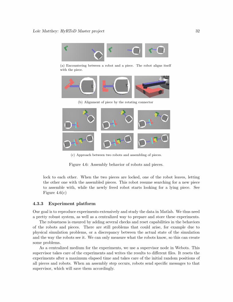
• When a robot receives a message from a free piece (i.e. they are in a small communica-tion range), it aligns with it, go towards it and carries it. This alignment uses relativerange and bearing offered by the emitter/receiver nodes of Webots. See Figure 4.6(a).
• While carrying the piece, the robot start moving around again, searching for anotherrobot with a compatible piece. Robots communicate with small range messages broad-casted at all time.
• When two robots carrying pieces come into communication ranges, they exchange mes-sage and look into the assembly plan. If their pieces correspond to no stored assemblystep, they moves away from each other.
• If their pieces can be assembled, the robot start an assembly procedure. According tothe piece type and the assembly plan, the robot first orient their pieces so as to show thegood connector in front. Again we use the relative range and bearing of emitter/receivernodes to perform that alignment. This step will be relaxed in a experimental scenarioto account for a random orientation of pieces for the assembly. See Figure 4.6(b).
• Then the robot align each other. The robot starts to approach, allowing the pieces to
Loıc Matthey: HyRToD Master project 32
(a) Encountering between a robot and a piece. The robot aligns itselfwith the piece.
(b) Alignment of piece by the rotating connector
(c) Approach between two robots and assembling of pieces.
Figure 4.6: Assembly behavior of robots and pieces.
lock to each other. When the two pieces are locked, one of the robot leaves, lettingthe other one with the assembled pieces. This robot resume searching for a new pieceto assemble with, while the newly freed robot starts looking for a lying piece. SeeFigure 4.6(c)
4.3.3 Experiment platform
Our goal is to reproduce experiments extensively and study the data in Matlab. We thus needa pretty robust system, as well as a centralized way to prepare and store these experiments.
The robustness is ensured by adding several checks and reset capabilities in the behaviorsof the robots and pieces. There are still problems that could arise, for example due tophysical simulation problems, or a discrepancy between the actual state of the simulationand the way the robots see it. We can only measure what the robots know, so this can createsome problems.
As a centralized medium for the experiments, we use a supervisor node in Webots. Thissupervisor takes care of the experiments and writes the results to different files. It resets theexperiments after a maximum elapsed time and takes care of the initial random positions ofall pieces and robots. When an assembly step occurs, robots send specific messages to thatsupervisor, which will save them accordingly.
Loıc Matthey: HyRToD Master project 33
4.3.4 Python world generator
Webots does not provide an easy way of varying the components of a given world. However,as we want to control easily the number of robots, pieces, the size of the arena and severalother parameters. Therefore, we created our own Webots world generator, in Python.
This world generator is available online on the mailing group of Webots, as it was buildto be easily extended. It takes the following inputs:
• A set of template files. They store parts of a classical Webots VRML world file, butwith added free parameters in them.
• A input XML file describing the world to create. This file defines which templates touse and how many instances of them to create and finally assigns values to the freeparameters.
It is easy to add new templates and extend this to different applications.This generator allows us to generate experimental worlds containing different numbers of
pieces and robots easily. We study for now a world with 5 pieces and 4 or 5 robots, and aworld with 15 pieces and 15 robots.
4.4 The robot transporters scenario
Characteristics: Lying pieces, robots carry and assemble them.This system represents either a self-assembly task if we abstract the robots, or a trans-
porting and assembly task. The pieces can not move and rely on the robots to create apuzzle.
4.4.1 Simulation results
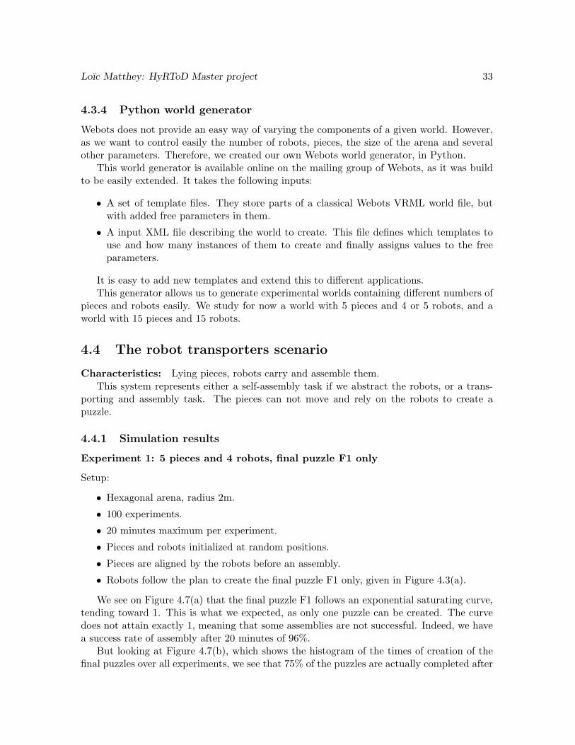
Experiment 1: 5 pieces and 4 robots, final puzzle F1 only
Setup:
• Hexagonal arena, radius 2m.
• 100 experiments.
• 20 minutes maximum per experiment.
• Pieces and robots initialized at random positions.
• Pieces are aligned by the robots before an assembly.
• Robots follow the plan to create the final puzzle F1 only, given in Figure 4.3(a).
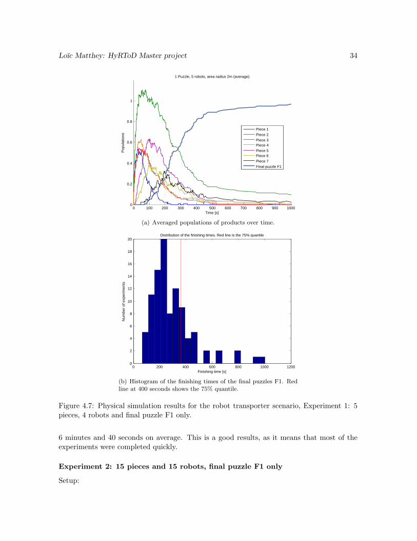
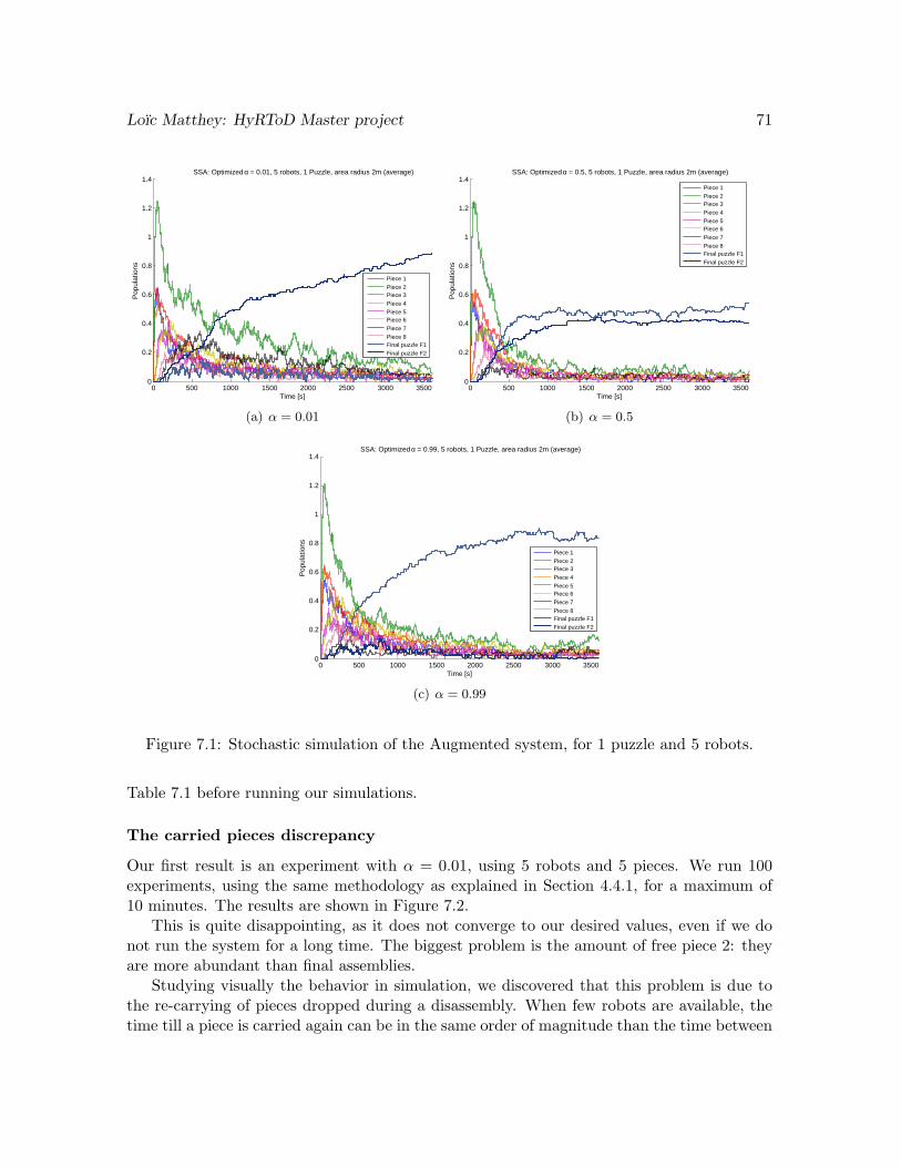
We see on Figure 4.7(a) that the final puzzle F1 follows an exponential saturating curve,tending toward 1. This is what we expected, as only one puzzle can be created. The curvedoes not attain exactly 1, meaning that some assemblies are not successful. Indeed, we havea success rate of assembly after 20 minutes of 96%.
But looking at Figure 4.7(b), which shows the histogram of the times of creation of thefinal puzzles over all experiments, we see that 75% of the puzzles are actually completed after
Loıc Matthey: HyRToD Master project 34
0 100 200 300 400 500 600 700 800 900 10000
0.2
0.4
0.6
0.8
1
1 Puzzle, 5 robots, area radius 2m (average)
Time [s]
Pop
ulat
ions
Piece 1Piece 2Piece 3Piece 4Piece 5Piece 6Piece 7Final puzzle F1
(a) Averaged populations of products over time.
0 200 400 600 800 1000 12000
2
4
6
8
10
12
14
16
18
20Distribution of the finishing times. Red line is the 75% quantile
Finishing time [s]
Num
ber
of e
xper
imen
ts
(b) Histogram of the finishing times of the final puzzles F1. Redline at 400 seconds shows the 75% quantile.
Figure 4.7: Physical simulation results for the robot transporter scenario, Experiment 1: 5pieces, 4 robots and final puzzle F1 only.
6 minutes and 40 seconds on average. This is a good results, as it means that most of theexperiments were completed quickly.
Experiment 2: 15 pieces and 15 robots, final puzzle F1 only
Setup:
Loıc Matthey: HyRToD Master project 35
• Hexagonal arena, radius 3m.
• 100 experiments.
• 20 minutes maximum per experiment.
• Pieces and robots initialized at random positions.
• Pieces are aligned by the robots before an assembly.
• Robots follow the plan to create the final puzzle F1 only, given in Figure 4.3(a).
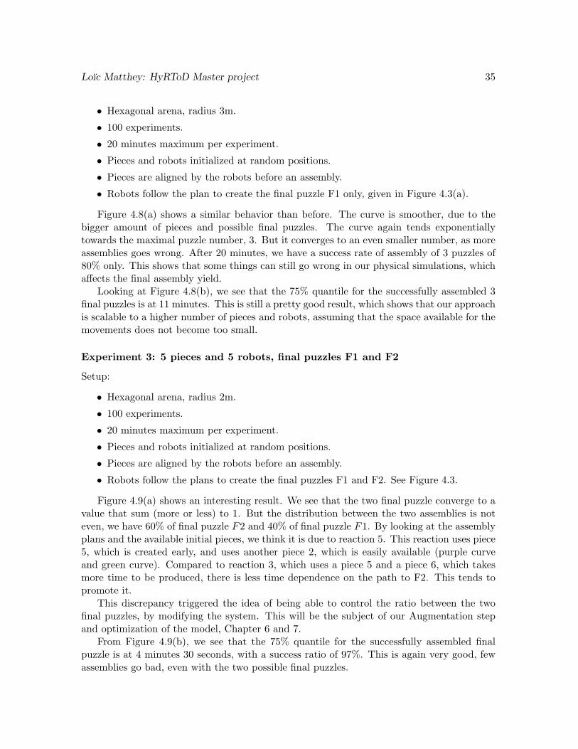
Figure 4.8(a) shows a similar behavior than before. The curve is smoother, due to thebigger amount of pieces and possible final puzzles. The curve again tends exponentiallytowards the maximal puzzle number, 3. But it converges to an even smaller number, as moreassemblies goes wrong. After 20 minutes, we have a success rate of assembly of 3 puzzles of80% only. This shows that some things can still go wrong in our physical simulations, whichaffects the final assembly yield.
Looking at Figure 4.8(b), we see that the 75% quantile for the successfully assembled 3final puzzles is at 11 minutes. This is still a pretty good result, which shows that our approachis scalable to a higher number of pieces and robots, assuming that the space available for themovements does not become too small.
Experiment 3: 5 pieces and 5 robots, final puzzles F1 and F2
Setup:
• Hexagonal arena, radius 2m.
• 100 experiments.
• 20 minutes maximum per experiment.
• Pieces and robots initialized at random positions.
• Pieces are aligned by the robots before an assembly.
• Robots follow the plans to create the final puzzles F1 and F2. See Figure 4.3.
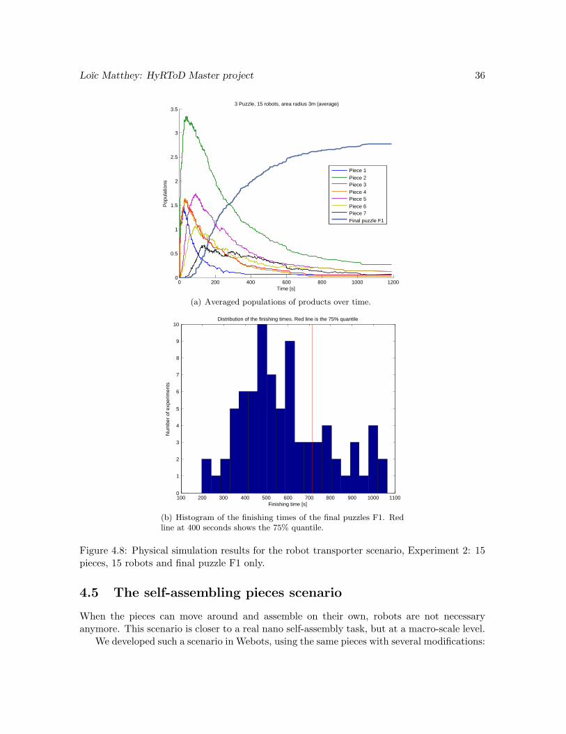
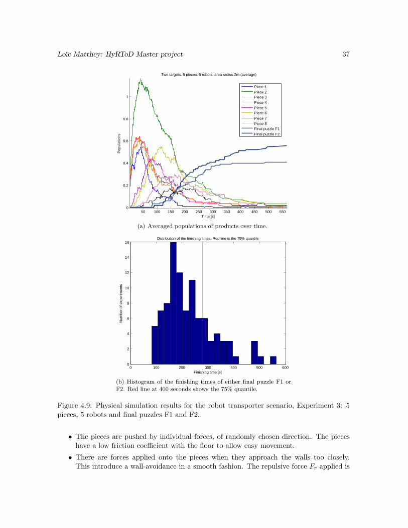
Figure 4.9(a) shows an interesting result. We see that the two final puzzle converge to avalue that sum (more or less) to 1. But the distribution between the two assemblies is noteven, we have 60% of final puzzle F2 and 40% of final puzzle F1. By looking at the assemblyplans and the available initial pieces, we think it is due to reaction 5. This reaction uses piece5, which is created early, and uses another piece 2, which is easily available (purple curveand green curve). Compared to reaction 3, which uses a piece 5 and a piece 6, which takesmore time to be produced, there is less time dependence on the path to F2. This tends topromote it.
This discrepancy triggered the idea of being able to control the ratio between the twofinal puzzles, by modifying the system. This will be the subject of our Augmentation stepand optimization of the model, Chapter 6 and 7.
From Figure 4.9(b), we see that the 75% quantile for the successfully assembled finalpuzzle is at 4 minutes 30 seconds, with a success ratio of 97%. This is again very good, fewassemblies go bad, even with the two possible final puzzles.
Loıc Matthey: HyRToD Master project 36
0 200 400 600 800 1000 12000
0.5
1
1.5
2
2.5
3
3.53 Puzzle, 15 robots, area radius 3m (average)
Time [s]
Pop
ulat
ions
Piece 1Piece 2Piece 3Piece 4Piece 5Piece 6Piece 7Final puzzle F1
(a) Averaged populations of products over time.
100 200 300 400 500 600 700 800 900 1000 11000
1
2
3
4
5
6
7
8
9
10Distribution of the finishing times. Red line is the 75% quantile
Finishing time [s]
Num
ber
of e
xper
imen
ts
(b) Histogram of the finishing times of the final puzzles F1. Redline at 400 seconds shows the 75% quantile.
Figure 4.8: Physical simulation results for the robot transporter scenario, Experiment 2: 15pieces, 15 robots and final puzzle F1 only.
4.5 The self-assembling pieces scenario
When the pieces can move around and assemble on their own, robots are not necessaryanymore. This scenario is closer to a real nano self-assembly task, but at a macro-scale level.
We developed such a scenario in Webots, using the same pieces with several modifications:
Loıc Matthey: HyRToD Master project 37
50 100 150 200 250 300 350 400 450 500 5500
0.2
0.4
0.6
0.8
1
Two targets, 5 pieces, 5 robots, area radius 2m (average)
16Distribution of the finishing times. Red line is the 75% quantile
Finishing time [s]
Num
ber
of e
xper
imen
ts
(b) Histogram of the finishing times of either final puzzle F1 orF2. Red line at 400 seconds shows the 75% quantile.
Figure 4.9: Physical simulation results for the robot transporter scenario, Experiment 3: 5pieces, 5 robots and final puzzles F1 and F2.
• The pieces are pushed by individual forces, of randomly chosen direction. The pieceshave a low friction coefficient with the floor to allow easy movement.
• There are forces applied onto the pieces when they approach the walls too closely.This introduce a wall-avoidance in a smooth fashion. The repulsive force Fr applied is
Loıc Matthey: HyRToD Master project 38
directed toward the center of the arena and an amplitude inversely proportional to thecurrent distance to the walls:
Fr ∼1(√
x2 + y2 −Rasin(π3 ))2 ·
(−x−y
)
Rasin(π3 ) is the radius of the incircle to the hexagonal arena of radius Ra.
• The pieces attracts each others in a small radius. This was introduced to improvethe encountering rate, which was not comparable to the one we had before. Indeed, acollision of two pieces is less likely than the encountering of two communication circlesas we had before. This force attracts the pieces for some time, and then repulse then,to mimic a missed assembly.
All these modifications create a scenario where the assembly rates are much smaller thanbefore, but which can still create some final puzzles. Unfortunately, due to robustness issues,we did not manage to get systematic experiments in time for that scenario. Its study will bedone in further works.
4.6 The mixed assembly scenario
We can combine the two last scenarios into this fully complex one. The pieces can movearound and assemble on their own, but can also be carried around and assembled by robots.
In order to make the carrying possible, the pieces stop moving when a robot is trying tograb them. Moreover, a free piece cannot interact with a carried piece. The robot has todrop it first.
This scenario closely resembles a biological process with enzymatic components. Thepieces assemble following their own dynamics, which are improved by the robots via theirspecific actions and orientation capabilities.
Again we did not manage to completely study this scenario. We leave it as further work,not without regrets.
Chapter 5 Mathematical model of thepuzzle test-case
5.1 Model definition
We introduce now the mathematical model used to represent our puzzle test-case system. Astold earlier, we use a chemical reaction network framework (see Section 3.2 for backgroundon this subject).
We only consider the robot transporters scenario, the other scenario can be modeled inthe same fashion.
We assign a reaction to each assembly step in the creation of the final puzzles. Lookingback at Figure 4.3, each numbered assembly step corresponds to a reaction in our chemicalreaction network. Furthermore, we add 4 new reactions, representing the grabbing of lyingpieces by the robots. The products and reactants are the different mid-assemblies, plus the3 lying free pieces and the robots. All reactions are second-order reactions, as they dependon the encountering of two different reactants upon reaction.
We obtain the following chemical reaction network (Equation (5.1)):
XR +Xf1
e1−→ X1 XR +Xf3
e3−→ X3
XR +Xf2
e2−→ X2 XR +Xf4
e4−→ X4
X1 +X2k1−→ X5 +XR X2 +X7
k4−→ XF1 +XR
X3 +X4k2−→ X6 +XR X2 +X5
k5−→ X8 +XR
X5 +X6k3−→ X7 +XR X6 +X8
k6−→ XF2 +XR (5.1)
XR is a robot, Xfi are the free lying pieces, Xk are the carried pieces and XFj the final
puzzles.The variables can be defined as the number of each piece type, where the number is a
continuous function of time [29]. This network can then be transformed in the followingassociated ODE system (Equation (5.2)):
Obviously, this notation is less compact, yet has the same meaning.We can also represent the network in matrix form:
x = SKy
S is the stoichiometric matrix, containing the stoichiometric coefficients mr and np as definedin Equation (3.1) in Section 3.2.1. K is the matrix of stochastic constant rates. y is a vectorof compounds, in our case the set of all bilinear terms in Equation (5.2) for example.
We can also relax the xR and xfi terms, if we decide to look only at the real assemblyprocess therein. Doing so is consistent if we assume that we have a big number of robots tocarry the pieces around, and that they grab the pieces very quickly compared to the actualassembly process. This approach is similar as doing a quasi-steady state simplification, fora multiscale system where the robots are acting quicker than the rest of the system. Such arelaxation simplifies the whole system and its analysis, we will use it in the next chapter.
5.1.1 Simulation of the model
We simulate our models using two different approaches:
1. ODE solving. We use Matlab to solve numerically the system (5.2), using a classicalode45. We use libSBML [57] for Matlab to write and read from SBML files onto ODEfiles.
2. Stochastic Simulation Algorithm. We use the StochKit toolbox [50], developed byPetzold et al. StochKit is a simulation framework for stochastic simulations written inC++. It allows a very fast exact simulations of chemical reaction networks.
Loıc Matthey: HyRToD Master project 41
5.2 Parameter fitting
5.2.1 Theoretical value of reaction rates
The chemical reaction network is easy constructed from the assembly plans considered, butwe still need to find values for the stochastic constant rates ki and el.
We decompose the stochastic constant rates as follows:
ki = pei · pai (5.3)
where pei is the probability of an encounter between two elements and pai the probabilityof successful assembly.
pai can be easily measured, or assumed to be 1 if the robots manage to align the piecescorrectly before each assembly step.
If we assume that our model is non-spatial, i.e. that the probability that two product areat a given position is independent of the time and uniformly distributed over the availablearena space, we can make an initial informed guess on the encountering probability. We takean approach used in [58, 59, 60], giving the following relation for the encountering probability:
pei ∼1
AtotalvrTw
id (5.4)
Where Atotal is the arena size, vr is the average speed of an element, T is the timestep(fixed to 1 in our case) and wid the width of detection of an element. This expression canactually be linked back to the literature on chemical process simulations [30, 41, 48]. Forchemical process, the probability of collision depends on the volume swept by one molecule,which gives the probability that another molecule will collide it in the next dt. Equation (5.4)is exactly the same, as shown on Figure 5.1. In our case, as we work in a 2D plan, we only havesurface swept, which is exactly given by the right part of (5.4). Dividing by the total arenasize and assuming the elements are distributed uniformly in the arena, this gives directly theprobability of encountering between two elements.
vrT
wd
Volume swept
Figure 5.1: Graphical interpretation of the encountering probability and link to the volumeswept used in chemical simulations.
In our test case, we measured vr over 50 simulation runs using the robot movementpattern described earlier, the average speed was 0.128m/s. Atotal is also easily computed(= 6(R2
√3
4 ), i.e. the sum of the six equilateral triangles of radius R). wid becomes the doubleof the communication radius between robots or pieces, as it defines the range for the start ofan assembly.
Loıc Matthey: HyRToD Master project 42
Rates verification
We checked this initial guess by measuring the encountering rates in Webots. We create aworld with one lying piece and one searching robot, we measure the time to encounter, over200 experiments. As discussed in the theory of chemical reaction networks, these times aredistributed following an exponential of the encountering probability. We load the times inMatlab, and fit an exponential distribution to get this probability (Figure 5.2).
0 100 200 300 400 500 600 700 8000
0.05
0.1
0.15
0.2
0.25
0.3
0.35Distribution of the Piece encountering times, 4 robots, area 2m
Time [s]
Per
cent
age
Experimental dataFitted exponential, p
e = 0.00876
Figure 5.2: Encountering times for the Webots experiment, with the fitted Matlab exponen-tial.
We also add “dummy” robots in the arena, that only avoid each other without lookingfor the piece. It measures the effect of overcrowding on the well-mixed property we’re tryingto ensure within our Webots simulation.
The results of the comparison between the theoretical and measured rates of encounteringare shown in Figure 5.3. We see that the theoretical guess is pretty accurate, even tough it isoverestimated when more robots are present. The added robots seems to disturb the capacityof a robot to encounter a piece. This can be due to the fact that the robots perturbs thetrajectories while avoiding each others, overcrowding some areas and forbidding the accessto others.
The same measurement was performed for robot to robot encountering and gave similarresults. We do not show it here.
5.3 Comparison with physical simulation
We simulate the chemical reaction network (5.1) using the two approaches presented inSection 5.1.1. Depending on the initial conditions for the number of robots and pieces, wehave different experiments, following Section 4.4.
Comparison between theoretical and measured probability
Figure 5.3: Comparison between the theoretical guess for the encountering probability pie andthe measured encountering probability in Webots. The red intervals represents the confidenceintervals for the fitted encountering probability.
Stochastic constant rates values
Through all these experiments, the stochastic constant rates el and ki take similar values,conditioned by specific parameters presented in each experiment setup.
Encountering rates el = 1Atotal
· vr · wpd ∀l ∈ {1..4}.
Reaction rates ki = pai · 1Atotal
· vr · wrd ∀i.
Arena size Atotal = 3 ·R2a ·√
32 .
Average speed vr = 0.128 measured in Webots.
Piece communication width wpd = 2 · 0.4m, pieces are set to communicate in a 40cmradius.
Robot communication width wrd = 2 · 0.6m, robots are set to communicate in a 60cmradius.
Probability of successful assembly pai depends on the experiment being studied, moreprecisely on the assembly plan used. We measured it in Webots, over 100 runs, for theassembly plan creating only the final puzzle F1 and for the assembly plan creating thefinal puzzles F1 and F2. Results will be specified in the experiments’ setup.
5.3.1 Experiment 1: 5 pieces and 5 robots, final puzzle F1 only
Setup:
Initial conditions: XR = 5, Xf1 = 1, Xf
2 = 2, Xf3 = 1, Xf
4 = 1, Xi = 0, XFk = 0.
Loıc Matthey: HyRToD Master project 44
Experiment duration: 20 minutes.
Number of experiments (Stochastic simulation only): 100.
Arena size: Ra = 2m.
Probability of successful assembly: all pai where more or less equal to 0.98. Thus we setpai = 0.98.
See Figure 5.4 for the comparison between the simulated chemical reaction networks andthe Webots physical simulation. The results from the Webots simulation are taken fromSection 4.4.1. We show the averaged populations over 20 minutes.
(b) Stochastic simulation vs physical Webots simu-lation
Figure 5.4: Comparison between the models simulations and the physical Webots simulationfor the puzzle test-case, scenario 1, experiment 1.
We see that they fit closely to the physical simulation. Two differences arise:
• The ODE simulation population values are too small, because of the slow copy numberof components (Figure 5.4(a)). When doing an ODE approximation, one assumes thatthe number of components is big enough so that using continuous numbers does nothave much effects. This is not the case here, where we work with numbers smaller than10. On the other hand, the Stochastic simulation accurately captures this property, asit works with discrete numbers.
• The stochastic simulation attains 1, whereas the physical simulation stays below (Fig-ure 5.4(b)). These results show that, while there are problems in the Webots simulation(pieces stuck together, blocked against the walls), this is not taken into account in themodel. We could modify the model by introducing ways of deactivating some piecesto try to fit this difference. But we do not take much interest in that for this currentwork.
Loıc Matthey: HyRToD Master project 45
5.3.2 Experiment 2: 15 pieces and 15 robots, final puzzle F1 only
Setup:
Initial conditions: XR = 15, Xf1 = 3, Xf
2 = 6, Xf3 = 3, Xf
4 = 3, Xi = 0, XFk = 0.
Experiment duration: 20 minutes.
Number of experiments (Stochastic simulation only): 100.
Arena size: Ra = 3m.
Probability of successful assembly: pai = 0.98.
Under the same assumptions than for experiment 1, see Figure 5.5 for the comparison inthis scenario.
(b) Stochastic simulation vs physical Webots simu-lation
Figure 5.5: Comparison between the models simulations and the physical Webots simulationfor the puzzle test-case, scenario 1, experiment 2.
The results are similar to experiment 1. With a higher number of elements, the ODEsimulation is closer to the correct physical simulation. The stochastic simulation is still veryaccurate but attains the maximal number of puzzles whereas the physical simulation convergeto a lower value.
5.3.3 Experiment 3: 5 pieces and 5 robots, final puzzles F1 and F2
Setup:
Initial conditions: XR = 5, Xf1 = 1, Xf
2 = 2, Xf3 = 1, Xf
4 = 1, Xi = 0, XFk = 0.
Experiment duration: 20 minutes.
Number of experiments (Stochastic simulation only): 100.
Loıc Matthey: HyRToD Master project 46
Reaction i 1 2 3 4 5 6pa
i 0.9777 0.9074 0.9636 0.9737 0.833 1.0
Table 5.1: Probability of successful assembly for experiment 3. Measured over 100 experi-ments.
Arena size: Ra = 2m.
Probability of successful assembly: Results of the measures are shown in Table 5.1. Wesee that now, the probabilities are not equal and depend on the assembly step. Es-pecially, the success of reaction 5, to create piece 8, is significantly smaller. pai is setaccordingly for each reaction i.
See Figure 5.6 for the results.
0 100 200 300 400 5000
0.2
0.4
0.6
0.8
1
1.2
Physical simulation and ODE Model: Two final puzzles, 1 Puzzle, 5 robots, arena radius 2m
Time [s]
Pop
ulat
ions
Physic SimulationODE Model
(a) ODE simulation vs physical Webots simulation
0 100 200 300 400 5000
0.2
0.4
0.6
0.8
1
1.2
Physical simulation and Stochastic Model: Two final puzzles, 1 Puzzle, 5 robots, arena radius 2m
Time [s]
Pop
ulat
ions
Physic SimulationStochastic Model
(b) Stochastic simulation vs physical Webots simu-lation
Figure 5.6: Comparison between the models simulations and the physical Webots simulationfor the puzzle test-case, scenario 1, experiment 3.
We see that the ODE model fails to capture the time to convergence, and underestimatesthe speed of variations. It also seems that they do not converge to the same values, whichcould be a problem. However, using the Stochastic simulation with the exact same rates, wesee that the fitting is much better. The low copy numbers again has a big impact on thecapacity to use the ODE model as an approximation.
But the rates we use for the ODE model produce a good fit when using the Stochasticsimulation, which shows that our model accurately describes the physical system’s dynamics.We thus think that, if the copy number is big enough, the analysis with the ODE modelshould be sufficient.
We confirm this hypothesis by performing the same two final puzzles experiment, with15 pieces and 15 robots and a bigger arena (like Experiment 2). The parameters are adaptedaccordingly. We obtain the results shown in Figure 5.7.
Loıc Matthey: HyRToD Master project 47
0 100 200 300 400 500 600 700 800 900 10000
0.5
1
1.5
2
2.5
3
3.5Physical simulation and ODE Model: Two final puzzles, 3 Puzzles, 15 robots, arena radius 3m
Time [s]
Pop
ulat
ions
Physic SimulationODE Model
(a) ODE simulation vs physical Webots simulation
0 100 200 300 400 500 600 700 800 900 10000
0.5
1
1.5
2
2.5
3
3.5Physical simulation and Stochastic Model: Two final puzzles, 3 Puzzles, 15 robots, arena radius 3m
Time [s]
Pop
ulat
ions
Physic SimulationStochastic Model
(b) Stochastic simulation vs physical Webots simu-lation
Figure 5.7: Modified experiment 3 with 15 pieces and 15 robots, to show the effect of a largercopy number.
This confirms our assumption that the only problem with the ODE model discrepancy ofconvergence is the low copy number. In this new scenario, the fitting of the ODE simulationis good and converge to the physical values (Figure 5.7(a)). This tells us that we can indeeduse the ODE as a model, but only for a copy number large enough. We will take advantageof that fact in the next chapter.
5.4 Final considerations
The comparison between the models and the Webots physical simulations shows a close fitof our model to the experimental data. It proves that this model is accurate for our test-caseand considered problem. The stochastic simulation captures the correct behavior when thenumber of elements is small, which is in accordance with the assumptions on algorithmsdifferences.
Therefore, we will use directly the model into an optimization process, before mappingback the new model onto the physical simulation. This approach makes sense, as thanksto the accuracy of our model, we can then hope that the physical simulation will behave inthe same way. The only constraint is that we need to work with big copy numbers with theODE, to avoid convergence problems.
Some problems are still present. For example, the initial guess for the encounteringprobability becomes wrong when the number of robots and pieces grows. The guess relies ona strong non-spatiality constraint, which our physical simulation can not ensure in severalcases. Our models do not capture the failures of the physical simulations, which hinder theoverall performance and reliability of the assembly process.
This page intentionally left blank.
Chapter 6 Chemical reaction networkscontrol and design
Having successfully modeled our puzzle test-case using a Chemical Reaction Network, weturn to the next step: modifying this model so that it behaves in a desired way.
This modification could be making it more efficient (i.e. optimizing it for a given metric)or just attaining a specific goal (i.e. create a specific final distribution). We define the controlproblem as follows:
Let a system of chemical reactions R, defined by a matrix of rate constants K, astoichiometry matrix S and a vector of products and reactants y. Let the initialcondition x0 be known also. What should be the matrix Kc so that the systemconverges as close as possible to a desired equilibrium X. Moreover, can we findthe matrix Kf that converge as close as possible to X at the fastest rate?
This is a design problem as well as an optimization problem. In the second proposition,we are optimizing for fast convergence subject to a constraint on the equilibrium.
This part has been done in close collaboration with Spring Berman.
6.1 Overview of possibilities
Our first goal was to use a previous optimization scheme used by S. Berman [3, 61], namelyoptimizing the Mixing-time of a Markov chain [62, 63, 64]. Unfortunately, our problem isnot a Markov chain. Our model is a continuous-time Markov process, with nonlinear rates.Actually, it is possible to represent it as a Markov chain, an approach taken by Klavins forhis optimization technique [14]: we have to consider every possible macro-states or markingof the system starting from an initial condition, by discretizing all possible values taken bythe products, and then creating or measuring the probabilities to jump from one macro-stateto another. Obviously, this approach runs into a combinatorial explosion when the numberof species and their populations increase, which forbids us from using it. Other approachesusing Markov chains [65, 66] are also abandoned because of this problem.
Therefore, we looked into the chemical reaction networks literature for an optimizationscheme taking advantage of the control we have on the stochastic constant rates.
We found papers focusing on the reachability of networks, namely knowing what parts ofthe state space could be attained knowing the system dynamics [67, 68, 69, 70, 71]. Theseworks apply more to bioreactors and show little interest designing the reaction rates and more
49
Loıc Matthey: HyRToD Master project 50
on controlling already present reactions. Other works, on the other hand, rely too much on acontrol theory methodology, for example by adding a feedback to the system [72, 73, 74, 75].As we want to modify only the rates, these were not helpful.
Eventually, we found an interesting study in [76]. The authors propose an analysis andoptimization of the rates of a chain of reactions, with respect to several objectives. Thoseobjectives closely resembles the two propositions we are trying to solve, we will therefore useideas from their work, although our approach is original. However, they are working withreaction chains, which offers simplifications and results that are not available for our morecomplex reaction network.
6.2 Methodology
6.2.1 Changes on our models
Starting from the chemical reaction network (5.1), we make several modifications in order tosatisfy our methodology:
1. We remove the robots from the system. We assume that the number of robots is biggeror equal to the number of pieces and that the robots find and carry the piece veryquickly with respect to the time between assemblies. Under those assumptions, we canremove the robots in a quasi steady-state assumption, looking only at the dynamics ofthe products.
2. We add backward reactions to every existing assembling reaction. They correspond tothe degradation of a product into its reactants. Such reactions are needed when we willprove that our new system has only one globally asymptotically stable equilibrium.
The new chemical reaction network is:
X1 +X2
k+1
k−1
X5 X2 +X7
k+4
k−4
XF1
X3 +X4
k+2
k−2
X6 X2 +X5
k+5
k−5
X8
X5 +X6
k+3
k−3
X7 X6 +X8
k+6
k−6
XF2 (6.1)
In the thermodynamic limit [28], the physical system represented by (6.1) can be ab-stracted to a linear ordinary differential equation (ODE) model:
Loıc Matthey: HyRToD Master project 51
x1 = −k+1 x1x2 + k−1 x5
x2 = −k+1 x1x2 − k+
5 x2x5 − k+4 x2x7 + k−1 x5 + k−5 x8 + k−4 xF1
x3 = −k+2 x3x4 + k−2 x6
x4 = −k+2 x3x4 + k−2 x6
x5 = k+1 x1x2 − k−1 x5 − k+
3 x5x6 + k−3 x7 − k+5 x2x5 + k−5 x8
x6 = k+2 x3x4 − k−2 x6 − k+
3 x5x6 + k−3 x7 − k+6 x6x8 + k−6 xF2
x7 = k+3 x5x6 − k−3 x7 − k+
4 x2x7 + k−4 xF1
x8 = k+5 x2x5 − k−5 x8 − k+
6 x6x8 + k−6 xF2
xF1 = k+4 x2x7 − k−4 xF1
xF2 = k+6 x6x8 − k−6 xF2
(6.2)
Define a matrix M ∈ R10×12 in which each entry mji, j = 1, ..., 10, of column mi isdefined as the coefficient of piece type j in complex i (0 if the piece type is absent). Forinstance, the column corresponding to the complex X1 + X2 is [1 1 0 0 0 0 0 0 0 0]T . Nowrepresent the rate associated with reaction (i, j) ∈ E as kij and define a matrix K ∈ R12×12
with entries:
Kij =
kji if i 6= j , (j, i) ∈ E ,0 if i 6= j , (j, i) /∈ E ,−∑
(i,l)∈E kil if i = j .(6.3)
Finally, define a vector y(x) ∈ R12 in which entry yi is the piece variable or products ofvariables associated with complex i:
Then the ODE model (6.2) can be written in the following form [77]:
x = MKy(x) , (6.5)
One set of conservation constraints on the piece quantities is:x3 − x4 = N1
x1 + x5 + x7 + x8 + xF1 + xF2 = N2
x2 + x5 + x7 + 2(x8 + xF1 + xF2) = N3
x3 + x6 + x7 + xF1 + xF2 = N4
(6.6)
where Ni, i = 1, ..., 4, are computed from the initial piece quantities.It should be possible to find the equilibrium points as closed form formulas, but our
attempts in that direction were unsuccessful. We thus propose another approach.
6.2.2 Approach
Our optimization relies on the following hypotheses:
1. The system (6.5) is deterministic and its dynamics depend only on the rates K and theinitial conditions.
Loıc Matthey: HyRToD Master project 52
2. The system, while nonlinear in xi, converge to an unique positive equilibrium given aninitial condition and a matrix K.
3. The system (6.5) is nonlinear in xi but linear in ki.
4. K governs the rate of convergence of the system.
5. MKy(x) = 0 only at the equilibrium point.
Hypothesis 1 derives from the definition of an ODE and on the fact that we keep thenetwork fixed during the system evolution. Hypothesis 2 will be proved in Section 6.2.3, itis a main result in the success of our approach. Hypothesis 3 comes from the observation ofthe system (6.2). Hypothesis 4 will be discussed in Section 6.2.4. Hypothesis 5 is discussedin Section 6.2.4.
Then, under those hypothesis, it is possible to find an objective function linear in ki,using MKy(xd) = 0 as a set of constraints on the desired converged values of xd and solveit using a convex optimization algorithm.
The complete derivation and discussion is presented in Section 6.2.4.
6.2.3 Convergence of chemical reaction networks
Theorem 1. System (6.2) subject to (6.6) has a unique equilibrium x > 0.
Proof. Each steady state of the system can be classified as either a positive steady state,{x | MKy(x) = 0, xi > 0 ∀i}, or a boundary steady state, {x | MKy(x) = 0, xi =0 for some i}, which can be found by solving y(x) = 0 [77].
From definition (6.4) of y(x), the boundary steady states for the system satisfy
It can be concluded that in each boundary steady state, all xi = 0 except for one of the fourcombinations of variables (x1, x3), (x1, x4), (x2, x3), (x2, x4). Since we only consider systemsthat can produce xF1 and xF2, it is not possible for the system to reach any of these steadystates; each one lacks two piece types needed for the final assemblies.
The deficiency δ of a reaction network has been introduced as a measure giving insightsand proofs on the stability and the existence of equilibrium of a class of reaction networks [78,79, 80, 81, 82, 83, 84]. It is one of the two attempts at proving convergence and stabilityof chemical reaction network, the other one is based on so-called species-reaction graphsanalysis [85, 86, 87, 88, 89].
δ is calculated has the number of complexes minus the number of linkage classes, eachof which is a set of complexes connected by reactions, minus the network rank, which is therank of the matrix whose rows are each obtained by subtracting a column of M associatedwith a reactant in a particular reaction from a column associated with a product [78]. Itcan be shown that each of the six linkage classes in our system has rank 1 and the rank ofthe entire network is 6; from this the deficiency of each linkage class is calculated to be 0
Loıc Matthey: HyRToD Master project 53
and the deficiency of the entire network is 0 as well. Also, we observe that no complex inany linkage class transforms into a complex in another linkage class. These properties, alongwith the fact that the system kinetics are mass-action, satisfy the criteria for applying theDeficiency One Theorem in [78], which gives the result that the system can have no morethan one positive steady state.
Now we must show that there exists a positive steady state, which would be unique bythe Deficiency One result. Since the network rank of the system is the sum of the ranks ofthe linkage classes, the linkage classes constitute a direct partition of the network [81]. Also,since each linkage class has deficiency 0 and is weakly reversible, meaning that there is areaction pathway connecting each pair of complexes, each linkage class contains exactly onepositive steady state by the Deficiency Zero Theorem [78]. By Lemma 8.2.3 of [81], theseproperties imply that the system admits a positive steady state.
We still lack a proof on the stability of this unique equilibrium. If the deficiency zerotheorem [78] can be extended to support not only weakly reversible but also block weaklyreversible networks, then we would get such a result. A remark in [88] support that fact, butwe did not manage to get a formal proof as of today. However, the empirical experiments weare doing show that the equilibrium is stable, so we will assume this fact from now on.
6.2.4 Design of optimal rates
We consider the problem of designing the assembly system described by model (6.2) subjectto (6.6) to produce desired quantities of pieces. The derivation is similar for other systems.
System and equilibrium definition
The assembly system will be most productive if it yields the target quantities as quicklyas possible. This objective will be posed as the design of a set of optimal rates k+
i , k−i ,
i = 1, ..., 6, for model (6.2) that minimizes the convergence time of the resulting system to atarget vector of piece quantities, xd.
Note that although the quantities of only the final assemblies, XF1 and XF2, may needto be specified in practice, the optimization problem requires that target quantities of inter-mediate components be defined as well, as will be discussed later in this section.
The rates k+i , k
−i can be chosen so that the assembly system yields a target piece distri-
bution xd > 0 starting from any initial distribution of pieces:
1. First, specify target numbers of the intermediate and final assemblies, xdi , i = 5, ..., 8.
2. Then define piece quantities xdj , j = 1, ..., 4, in terms of these numbers according to theconservation equations (6.6).
3. Finally define yd = y(xd) according to definition (6.21).
This vector yd represents the steady-state quantities of the pieces and piece productsassociated with each complex. If the system described in the form (6.5) converges to yd,then it converges to the target quantities xdi , i = 5, ..., 8, since eight components of yd are
Loıc Matthey: HyRToD Master project 54
equal to these variables. Convergence to xdj , j = 1, ..., 4 is also ensured since each of thesequantities is a function of xdi , i = 5, ..., 8 by conservation laws.
By Theorem 1, model (6.2) always converges to a single positive equilibrium y. Therefore,system convergence to yd can be guaranteed by specifying that y ≡ yd through the followingconstraint on the rate matrix K in model (6.5):
MKyd = 0 . (6.8)
To control more easily the goal in term of final puzzles, we introduce the fraction α:
α =xF1
xF1 + xF2(6.9)
The target final assemblies can be defined in such a way that their sum, xF1+xF2, is constantand the fraction α is directly a tunable parameter. The sum xF1 + xF2 is expressed in termsof a conservation law, which means that one of the target quantities xdi , i ∈ {1, ..., 4}, must beimplicitly defined. For instance, using the third conservation equation in (6.6) and a targetvalue for xd2:
xdF1 = 12 α
(N2 − (xd2 + xd5 + xd7 + 2xd8)
)(6.10)
xdF2 = 12 (1− α)
(N2 − (xd2 + xd5 + xd7 + 2xd8)
), (6.11)
Whatever the selection of independent piece quantities, it must be ensured that theremaining piece quantities are positive to have a feasible xd (positive equilibrium).
Convergence time
Now we consider the aspect of minimizing the convergence time of the system to the targetequilibrium xd. We can define measures of this time by reformulating the system in termsof new variables. Define vj , j = 1, ..., 6, as the difference between the forward and reversefluxes associated with reaction j in system (6.1).
For instance, if we label reaction 1 as the one in which X1 + X2 is the reactant and X5
is the product, then v1 = k1x1x2 − k2x5. Let v(x) = [v1 ... v6]T . Denote the stoichiometricmatrix of the system by S ∈ R10×6, which is defined such that model (6.2) can be writtenas [90]:
x = Sv(x) . (6.12)
Our assembly system is similar to a model of a biochemical network with mass actionkinetics. The dynamical properties of such networks are often analyzed by linearizing theODE model of the system about a steady state and studying the properties of the associatedJacobian matrix J = SG, where the entries of G are gij = dvi/dxj (see [91] for an overviewand further references).
Denoting the eigenvalues of J by λi, τi = 1/|Re(λi)| are measures of the characteristictimes, referred to as relaxation times, in which different modes (dynamically independentvariables) of the the system converge to a stable steady state after perturbation [92, 91].
Loıc Matthey: HyRToD Master project 55
Since the λi are negative at a stable steady state, one way to yield fast convergence isto choose rates ki that minimize the largest negative λi, as was done for a linear chain ofenzymatic reactions in [76].
However, in our system it is very difficult to find analytical expressions for the λi, so wemust explore other ways of quantifying the convergence time.
Various measures of average relaxation times in biochemical networks have been defined,but they are applicable only under certain conditions, such as a linear reaction sequence [93].For instance, one such measure was minimized in the optimization of rates for the linear chainin [76]. For our system, we can use a general estimate of the relaxation time for each reactionj that is given in [90]. It is derived by linearizing the system model around its equilibriumpoint, which in our case is the target distribution xd enforced by equation (6.8):
τj =
(12∑i=1
(−sij)dvjdxi
)−1
(6.13)
This expression is evaluated at xd. Since each reaction j in system (6.1) is of the form
Xk+Xl k+
j
k−jXm, the net flux vj is k+
j xkxl−k−j xm, and the entries of column j in S are all
0 except for skj = slj = −1 and smj = 1. Thus, taking advantage of this fact and applyingequation (6.13) at xd, we get that the relaxation time for each reaction is
τj = (k+j (xdk + xdl ) + k−j )−1 . (6.14)
Which gives us a measure of speed of convergence.
Objective functions
Define k ∈ R12 as the vector of all rates k+i , k
−i . Using characterization (6.14) of reaction
relaxation times, we define two possible objective functions f : R12 → R to maximize in orderto produce fast convergence to xd.
The first is the average inverse relaxation time,
fave(k) = 110
10∑j=1
τ−1j . (6.15)
The second is the minimum inverse relaxation time,
fmin(k) = min{τ−11 , . . . , τ−1
10 } . (6.16)
Convex program definition
Finally, we map the rates onto actual adjustable parameters of the physical assembly system.Those adjustable parameters will be defined as the optimization variables.
Loıc Matthey: HyRToD Master project 56
Backward rates Each reverse rate k−j will be defined simply as a probability per unit timeof breaking up an assembly, p−j ∈ {0, 1}, which can be adjusted:
k−j = p−j (6.17)
Forward rates We use the formula (5.3) defined in Section 5.2.1. We extend it by addinga probability of starting the assembly p+
j ∈ {0, 1} which can be adjusted:
k+j = pej · paj · p+
j (6.18)
pej is the encountering probability defined by (5.4), dependent on some parameters andpaj is the assembly success rate, which we measure as explained in Section 5.3.
Let p ∈ R12 be the vector of all adjustable probabilities, p+j and p−j . Then we define an
optimization Problem P as follows:
P: maximize f(k(p))
subject to MK(p)yd = 0, 0 ≤ p ≤ 1 .
Depending on the objective function used, we define Problem P1 and Problem P2:
P1: maximize fave(k(p))
subject to MK(p)yd = 0, 0 ≤ p ≤ 1 .
P2: maximize fmin(k(p))
subject to MK(p)yd = 0, 0 ≤ p ≤ 1 .
Since this problem can be formulated as the minimization of a linear combination of theentries of p subject to a set of linear equality and inequality constraints on p, it is a linearprogram, which can be solved efficiently.
6.2.5 Optimization implementation
In order to optimize the convex programs P1 and P2, we use a framework for Matlab,YALMIP[94]. It allows us to define our optimization variables, objective function and con-straints and to apply a semidefinite programming solving algorithm, running in polynomialtime [94].
6.3 Results and limitations
We start with problem P1, which uses the first objective function fave, optimizing the av-erage inverse relaxation time. We take the system (6.1) and optimize it according to ourmethodology:
Loıc Matthey: HyRToD Master project 57
• As discussed in Section 5.3.3, and because our optimization rely on an underlyingODE approximation, we use an initial condition with a big copy number of pieces toavoid convergence problems. We use 60 pieces {1, 3, 4, 5}, 120 pieces 2 and no othermid-assemblies.
• For the forward rates, we assume that we can only optimize the probability of startingan assembly, p+
j . This probability comes in addition to the probability of encounterand the probability of successful assembly, as shown in Equation (6.18). It can takevalues from 0 to 1.
• For the backward rates, we optimize the probability of breaking up an assembly p−j , asEquation (6.17). It can take values from 0 to 1.
• Our goal is to control the ratio α between the final number of F1 and F2 puzzles,Equation (6.9). The converged number of other pieces are set to the smaller values stillconsistent with conservation laws and non-negativity constraints.
We optimize the system for α ∈ {0.01, 0.02, 0.03, . . . , 0.99} and store the obtained ratesfor all 6 reactions.
It turns out that nearly all rates keep constant values. All the forward rates are put totheir maximal values. Backward rates all take constant positive values, except the backwardrates of reactions 4 and 6, which vary continuously with respect to α. Table 6.1 displays theoptimized probabilities.
Table 6.1: Values of optimized rates for varying α, under objective function P1 for system(6.1). Continuous rates evolve continuously with respect to α.
The case of the continuously varying rates is very interesting. Those rates correspondsto the backward reaction coming from the two final puzzles F1 (reaction 4) and F2 (reaction6). Their evolution with respect to α is shown in Figure 6.1.
Having constant rates for every reaction except those two give several informations:
• The network is highly flexible, allowing every ratio of final puzzles only by changing twospecific backward rates. The non final reactions are kept to an activity low enough soas not to destroy to yield, but still high enough to be able to redistribute the materialswhen the final reactions are breaking up the final puzzles to converge to a desired ratio.Controlling only the disassembly rate of the two final puzzles is enough to attain anyratio α, while optimizing the yield and time to convergence.
• All the forward rates are put to their maximum value. This could show that using non-maximum forward rates decreases the convergence rate, but further tests about thathypothesis are necessary. In an informal discussion, G. Mermoud confirmed similarresults in previous works of his with self-assembly processes.
Loıc Matthey: HyRToD Master project 58
0 0.2 0.4 0.6 0.8 10
0.005
0.01
0.015
0.02
0.025
0.03
0.035
α = xF1
/(xF1
+xF2
)
Rat
es
Rates from Problem P1 that change with α
k
4−
k6−
Figure 6.1: Backward rates changing continuously with respect to α under objective functionP1 for system (6.1).
Doing the optimization of problem P2, under objective function fmin leads to slightlydifferent results. This time the forward rates and backwards rates of reactions 4 and 6 arevarying continuously. The forwards rate are not all maximum. Table 6.2 presents the resultsfor P2.
Table 6.2: Values of optimized rates for varying α, under objective function P2 for system(6.1). Continuous rates evolve continuously with respect to α.
Again with that objective function, the real control of the ratio α is carried on by thelast two reactions in the construction of the final assemblies. This time the forward rateshave a stronger role in that, but this has yet to be verified that this method is better. SeeFigure 6.2 for the continuous variation of rates with respect to α.
6.3.1 Comparison between objective functions and strategies
To compare the two functions, we plot the time-evolution of the ratio of the final puzzles F1and F2 for three different α: 0.1, 0.5 and 0.9, see Figure 6.3 a), c) and e). The horizontaldotted lines show the target ratios and both objective function are shown (plain for P1,dashed for P2).
We see that P1 is converging quicker than P2 to the equilibrium for α = 0.1 and α = 0.9,but is slower for α = 0.5. It is still unclear if it is only due to the values of the forward rates,as hypothesized. The overall speed of convergence is actually pretty slow, especially whentrying to produce 50% of both puzzles. This could be problematic, but is in fact linked tothe global behavior of the system, as we show now.
Loıc Matthey: HyRToD Master project 59
0 0.1 0.2 0.3 0.4 0.5 0.6 0.7 0.8 0.9 10
1
2
3
4
5
6
7
8
9x 10⁻³
α = xF1
/(xF1
+xF2
)
Rat
es
Rates from Problem P2 that change with α
k
4+ k
4− k
6+ k
6−
Figure 6.2: Forward and backward rates changing continuously with respect to α underobjective function P2 for system (6.1).
Looking at semi-logarithmic plots of the same data, Figure 6.3 b), d) and f), we clearlysee two regime of convergence:
• A quick convergence to an unique equilibria, independent of the chosen α, till t = 102s.We hypothesize that this equilibrium depends on the network topology and forwardrates.
• A “redistribution” regime starting from there, which makes the system converge to thefinal α desired. This regime is much slower than the first one. The final reactions withoptimized rates only act during that regime.
If we think in the state space of final assemblies, it means that the system first convergequickly to its intrinsic equilibrium, and then moves around slowly due to the redistributionof final puzzles until it arrives to the desired equilibrium.
This is a very interesting and quite counterintuitive result, as one might think that itwould be best to go directly towards the desired equilibrium. The optimization process weuse seems to point out that going quickly to the intrinsic equilibrium and then moving fromthere is a better strategy. Of course, this might be an artifact of the linear optimization wedo, so a verification with another optimization process should be performed. This will bedone in further works.
6.3.2 Online adaptation of the desired final puzzles ratio
We finish by showing the application of the rate optimization to the “green manufacturing”process shortly presented in Section 4.1. A “green manufacturing” process is a direct appli-cation of the flexibility offered by a non-specific assembly task. In that process, we reusefinished products (in our case, final puzzles) in order to create new products, depending onthe current demand. We “recycle” the products into new ones. This is possible because
Loıc Matthey: HyRToD Master project 60
0 0.5 1 1.5 2 2.5 3
x 104
0
0.1
0.2
0.3
0.4
0.5
0.6
0.7
0.8
0.9
1
Time
x F1 a
nd x
F2
xF1
and xF2
vs. time, α = 0.1
x
F1, P1
xF2
, P1
xF1
, P2
xF2
, P2
(a) α = 0.1, Linear x axis.
100 101 102 103 1040
0.1
0.2
0.3
0.4
0.5
0.6
0.7
0.8
0.9
1
Time
x F1 a
nd x
F2
xF1
and xF2
vs. time, α = 0.1
xF1
, P1
xF2
, P1
xF1
, P2
xF2
, P2
(b) α = 0.1, Log x axis.
0 0.5 1 1.5 2 2.5 3
x 104
0
0.1
0.2
0.3
0.4
0.5
0.6
0.7
0.8
0.9
1
Time
x F1 a
nd x
F2
xF1
and xF2
vs. time, α = 0.5
x
F1, P1
xF2
, P1
xF1
, P2
xF2
, P2
(c) α = 0.5, Linear x axis.
100 101 102 103 1040
0.1
0.2
0.3
0.4
0.5
0.6
0.7
0.8
0.9
1
Time
x F1 a
nd x
F2
xF1
and xF2
vs. time, α = 0.5
x
F1, P1
xF2
, P1
xF1
, P2
xF2
, P2
(d) α = 0.5, Log x axis.
0 0.5 1 1.5 2 2.5 3
x 104
0
0.1
0.2
0.3
0.4
0.5
0.6
0.7
0.8
0.9
1
Time
x F1 a
nd x
F2
xF1
and xF2
vs. time, α = 0.9
x
F1, P1
xF2
, P1
xF1
, P2
xF2
, P2
(e) α = 0.9, Linear x axis.
100 101 102 103 1040
0.1
0.2
0.3
0.4
0.5
0.6
0.7
0.8
0.9
1
Time
x F1 a
nd x
F2
xF1
and xF2
vs. time, α = 0.9
xF1
, P1
xF2
, P1
xF1
, P2
xF2
, P2
(f) α = 0.9, Log x axis.
Figure 6.3: Comparison of convergence of final assemblies over time after optimizing P1 andP2. Time unit is seconds.
Loıc Matthey: HyRToD Master project 61
our system possess the capabilities to create both products, and because we fix what it issupposed to create by optimizing the rates of assembly as shown in this chapter.
We show such an example of online adaptation to a new goal, by simulating the followingexperiment:
• Through all this experiment, we use the optimized goals under objective function P1,see Table 6.1 and Figure 6.1.
• We initialize the system with a first goal of a 60% ratio of final puzzle F2 (α = 0.4).We let the system run till t1 = 1000s.
• We change the rates to the one optimized to create a ratio of 99% final puzzle F1(α = 0.99). We let the system run till t2 = 6000s.
• We change the rates to a goal of 99% of final puzzle F2 (α = 0.01). We let the systemrun till t3 = 11000s.
• We change for the last time the rates for a goal of 50% of each final puzzle (α = 0.5).We let the system run till t4 = 21000s.
The result is shown in Figure 6.4. We see that the system is capable of adapting smoothlyto abrupt new commands in the desired targets. It attains the desired ratio when converged.The convergence time is pretty slow when approaching the desired ratio, yet the disruptionof the previous steady state occurs quickly. The target of 50% of both puzzles is slower toattain.
0 0.2 0.4 0.6 0.8 1 1.2 1.4 1.6 1.8 2
x 104
0
0.1
0.2
0.3
0.4
0.5
0.6
0.7
0.8
0.9
1
Time [s]
Pro
port
ion
of fi
nal p
uzzl
es
System adaptation to change of rates
X1
X2
X3
X4
X5
X6
X7
X8
XF1
XF2
Figure 6.4: Change of reaction rates during an experiment. System adapts smoothly to thenew equilibrium. Rates are changed at the times indicated by the dotted vertical lines. Firstgoal is 60% of F2, second is 100% of F1, third is 100% of F2 and fourth is 50% of each.
A good result is the speed of adaptation to new commands, and the strong redistributioneffect of commands asking for near 100% ratios. We think it is also possible to design acontrol policy stabilizing quicker to a slow target (50% for example) by switching between
Loıc Matthey: HyRToD Master project 62
a 100% F1 and a 100% F2 command, slowly damping the oscillations till we attain thedesired distribution. This is a similar approach to the one shown in [95, 96] for the controlof switching in E. Coli. More tests are still necessary to assess the validity of this process,but the behavior we obtain already offers us a large variety of adaptable behaviors.
6.4 Beyond control, direct optimization of the plan?
Can our optimization scheme optimize directly a set of assembly plans? We addressed thatproblem in Section 3.3, while speaking about the optimal plans. In his work, Klavins [14]constructs an optimal assembly plan using graph grammars. This is a discrete optimization,i.e. choosing what reactions to use to build an optimal plan. On the other hand, givenoptimized rates, it is possible to see if some reactions are promoted or deactivated. Thiscorresponds to a continuous optimization of the assembly plan, effective while the system isbehaving. We think our optimization is able to perform such a continuous optimization. Wewill alter our model in order to test that hypothesis.
We add new assembly steps to create additional pathways to the final assemblies. Inaddition to plans shown in Figures 4.3, we add two new plans, that reuse parts of the oldones, see Figures 6.5. The new assembly steps are shown in boldface. We call those new plans“sequential plans”, as they assemble one piece at a time without parallel processes. Our goalis to see how the algorithm treats these new pathways, more precisely if it “shuts down” theones which are not optimal or useful. Remark that we do not consider the case of all possibletypes of reactions in the system, but only a selected sub-set of them. Using the complete setfor the optimization of the plan is let for further work.
The 4 added assembly steps translate into the following reactions to be added to the set(6.1):
X3 +X5
k+7
k−7
X9 X3 +X8
k+9
k−9
X10
X4 +X9
k+8
k−8
X7 X4 +X10
k+10
k−10
XF2 (6.19)
With these added reactions, the ODE equations for the system are:
Loıc Matthey: HyRToD Master project 63
1
2
3
4
5
97
2
F1
1
7
8
4
(a) New added first final puzzle plan
1
2
3
4
5
108
F2
2
10
1
5
9
(b) New added second final puzzle plan
Figure 6.5: New plans created by adding 4 new assembly steps, written in boldface. We callthose plans the “sequential plans”, as they act by assembling one piece after another withoutparallel processes.
x1 = −k+1 x1x2 + k−1 x5
x2 = −k+1 x1x2 − k+
5 x2x5 − k+4 x2x7 + k−1 x5 + k−5 x8 + k−4 xF1
x3 = −k+2 x3x4 + k−2 x6 − k+
7 x3x5 + k−7 x9 − k+9 x3x8 + k−9 x10
x4 = −k+2 x3x4 + k−2 x6 − k+
8 x4x9 + k−8 x7 − k+10x4x10 + k−10xF2
x5 = k+1 x1x2 − k−1 x5 − k+
3 x5x6 + k−3 x7 − k+5 x2x5
+k−5 x8 − k+7 x3x5 + k−7 x9
x6 = k+2 x3x4 − k−2 x6 − k+
3 x5x6 + k−3 x7 − k+6 x6x8 + k−6 xF2
x7 = k+3 x5x6 − k−3 x7 − k+
4 x2x7 + k−4 xF1 + k+8 x4x9 − k−8 x7
x8 = k+5 x2x5 − k−5 x8 − k+
6 x6x8 + k−6 xF2 − k+9 x3x8 + k−9 x10
x9 = k+7 x3x5 − k−7 x9 − k+
8 x4x9 + k−8 x7
x10 = k+9 x3x8 − k−9 x10 − k+
10x4x10 + k−10xF2
xF1 = k+4 x2x7 − k−4 xF1
xF2 = k+6 x6x8 − k−6 xF2 + k+
10x4x10 − k−10xF2
(6.20)
Loıc Matthey: HyRToD Master project 64
Like system (6.2), this system can be written in the form (6.5). In this case, the vectorof complexes is defined as
One set of conservation constraints on the piece quantities in this system is:x1 + x5 + x7 + x8 + xF1 + xF2 + x9 + x10 = N5
x2 + x5 + x7 + 2x8 + 2xF1 + 2xF2 + x9 + 2x10 = N6
x3 + x6 + x7 + xF1 + xF2 + x9 + x10 = N7
x4 + x6 + x7 + xF1 + xF2 = N8
(6.22)
where Ni, i = 5, ..., 8, are computed from the initial piece quantities.
6.4.1 Optimized rates and induced effective plan
We apply our optimization procedure with Problem P1 and P2 as before. The results for theconvergence are shown in Figure 6.6. As Problem P2 is quicker in general and shows moreinterest dynamics, we will only study it for the rest of this section.
The resulting probabilities p+i , p
−i for problem P2 are nearly all continuously varying. The
only exceptions are p+3 , p+
6 and p+9 which are all at 1.0. The variation of the rates for the
values of α are shown in Figure 6.7.Looking at the values of the rates at specific positions, we can make observation on
the actual plan promoted by the optimization. The reactions, though still present, will bepromoted or deactivated when their corresponding forward and backward rates are modi-fied. This corresponds to a continuous optimization of the plan, in contrast with a discreteoptimization performed by Klavins[14].
In general, the value of the rates show the following hierarchy between reactions andpathways:
• k+2 is small and k−2 is big compared to other rates. This deactivates Reaction 2.
• To compensate the absence of piece 6, the sequential pathways represented by reactions7 and 8 for F1 and reactions 9 and 10 for F2 are really active.
• The small amount of pieces 6 that would result from breaking of assemblies are quicklyreuse via the reactions 3 and 6, which have of full forward rate, or destroyed by thebackward rate of reaction 2.
We see three different regimes for the rates, and the resulting continuous assembly plans:
1. Near α = 0.1, the only changing rates are k+4 and k−4 . They are changing toward a
deactivation of Reaction 4, which is the only one creating F1 puzzles. The networkthen automatically tends to create more F2 puzzles, which seems to be a constantcharacteristic of the system we are studying.
Loıc Matthey: HyRToD Master project 65
100 101 102 103 1040
0.16
0.33
0.5
0.66
0.83
1
Time
x F1 a
nd x
F2
xF1
and xF2
vs. time, α = 0.1
x
F1, P1
xF2
, P1
xF1
, P2
xF2
, P2
(a) α = 0.1, Log x axis.
100 101 102 103 1040
0.16
0.33
0.5
0.66
0.83
1
Time
x F1 a
nd x
F2
xF1
and xF2
vs. time, α = 0.5
x
F1, P1
xF2
, P1
xF1
, P2
xF2
, P2
(b) α = 0.5, Log x axis.
100 101 102 103 1040
0.16
0.33
0.5
0.66
0.83
1
Time
x F1 a
nd x
F2
xF1
and xF2
vs. time, α = 0.9
x
F1, P1
xF2
, P1
xF1
, P2
xF2
, P2
(c) α = 0.9, Log x axis.
Figure 6.6: Expanded system. Comparison between the two objective functions P1 and P2when showed with semi-logarithmic x axis.
2. Between α = 0.2 and α = 0.8, the rates k+4 and k−6 seems to have to most effect. They
act by promoting the creation of F1 and slowing the creation of F2. During that period,the networks tends to produce a 50% ratio by itself, as shown by the convergence profilein Figure 6.6(b): the first convergence arrives close to a 50%, no redistribution is needed(to compare with Figure 6.3(d) of the previous system)
3. Near α = 0.9, the behavior changes dramatically. Reactions 7, 8 and 4, leading to thecreation of F1 are promoted extensively (increase in forward rate, decrease in backwardrate). At the same moment, reactions 6 and 10, creating F2, are deactivated. Thispromotes the creation of F1 puzzles.
We see then that this optimization works with these general tendencies:
• Remove assembly 6 from the possible pool of pieces, to liberate all initial pieces forother reactions. This means removing the initial plans we were using an use the newintroduced one, see Figure 6.5
• Use the sequential steps to create the final puzzles. This is a counter-intuitive results,but it may be linked to an added flexibility with having a large pool of initial pieces,
Loıc Matthey: HyRToD Master project 66
0 0.2 0.4 0.6 0.8 10
1
2
3
4
5
6
7
x 10−3
α = xF1
/(xF1
+xF2
)
Rat
es
Forward rates from Problem P2 that change with α
k1+
k2+
k4+
k5+
k7+
k8+
k10+
(a) Forward rates varying continuously
0 0.2 0.4 0.6 0.8 10
0.002
0.004
0.006
0.008
0.01
0.012
α = xF1
/(xF1
+xF2
)
Rat
es
Reverse rates from Problem P2 that change with α
k1−
k2−
k3−
k4−
k5−
k6−
k7−
k8−
k9−
k10−
(b) Backward rates varying continuously
Figure 6.7: Optimized rates of expanded system under problem P2, for α ∈ 0.01, 0.99.Remark: k−6 curve is the same as k−3 .
that can be used at precise assembly steps without temporal dependences betweenreactions.
• Modify the reactions leading to the final assemblies to change the ratio, and do nottouch the “general” part of the system. This is in agreement with the behavior weobserved in last section.
Loıc Matthey: HyRToD Master project 67
• As the system is more prone to create F2 than F1, it is easier to control the system inone direction than the other. To create a big ratio of F1, the overall behavior of thesystem is changed, leading to a nearly new plan. This plan correspond to the sequentialone we added in Figure 6.5(a).
So in conclusion, it is possible to get insights into the kind of behaviors and continuousplans promoted by the optimization. The algorithm promoted the use of sequential plans,with the addition of “rewiring” the system when the goal to attain is in contradiction withthe intrinsic behavior of the system (e.g. to create the big ratio of F1).
These results are not that intuitive, i.e. one would think that using parallel assemblysteps is more efficient for the convergence time. But comparing the results, we see thatthe “sequential plan” is much quicker for α = 0.5, and slightly worse for the two others(4 · 104 seconds instead of 3 · 104 seconds). However, it has to be checked that such an opti-mization would give similar results for a more complicated set of assembly plans, especiallythe “full set assembly plan” consisting of all possibles reactions of the system.
This page intentionally left blank.
Chapter 7 Augmented assembly imple-mentation
7.1 Top-bottom approach
This chapter will cover the last step in our methodology: going back from the modified modelto the physical system, while applying the introduced modifications.
This is a Top-bottom approach, which is of growing interests nowadays. This methodbecomes interesting when the behavior of the low-level parts is hard to create, when theglobal behavior does not simply follow from the behavior of the low-level parts or when wewant to low-level parts to follow directives given at a higher level.
In our case, our problem is that we do not know how to modify the behavior of thelow-level parts (i.e. the robots and pieces and their interactions) so as to create a high-levelgoal. When working on the mathematical model level, we can define our high-level goalsmore easily.
The main difficulty of this approach is to create a mapping from the high-level to thelow-level.
7.2 Rates mapping
In our case, this problem is actually simpler, because we have a direct dependance betweenrates in the mathematical model and behavior of the robots.
Especially, we created a bidirectional relation between the stochastic constant rates ofour mathematical model and physical capacities or behavior of our robots and pieces. Themapping from the model to the physical system is thus straightforward:
Backward probability p−i : A robot carrying an assembly draws a random number at eachtimestep and compare it to the p−i corresponding to its carried assembly i. Precisely:
if U(0, 1) < p−i · T → disasssemble assembly i.
where T is the timestep of the physical simulation. This is needed because p−i is abackward rate per second.
Forward probability p+i : As shown in Equation (6.18), this probability is used when an
assembly is starting. Before actually doing the assembly, a random number is drawnand compared to it:
Table 7.1: Set of optimized probabilities used for the Top-down mapping. Reactions fromsystem (6.1).
When a disassembly is triggered, the carrying robot drops one of the assemblies on theground and resume searching with the remaining carried assembly. This dropped assemblyshould then be grabbed by another robot in order to be attached again.
These behavior should directly create the change of rates needed for the modified math-ematical model.
When such a bidirectional mapping is not that easily available, we have to discover thatmapping. A possibility would be to create an iterative process between a modification oflow-level parameters and a measure of the resulting rate modification in the model.
7.3 Augmentation results and implications
We choose to implement the set of optimized probabilities shown in Table 7.1. It has beenfound by solving problem P1 in Section 6.3.
7.3.1 Stochastic model
We start by verifying the behavior with the stochastic simulation of our model with backwardrates. We modify Equation (5.2) to add the backward reactions while still modeling the robotsand free pieces. Our model takes into account the dropped pieces when a disassembly occurs.The results for 1 puzzle are shown in Figure 7.1. The results are similar for 3 puzzles, so wedo not show them here.
According to these simulations, the optimized rates for the simplified system (6.1) trans-lates into the same global optimized behavior when used on the complete system with robotsand free pieces. It manages to create the target ratio α quite successfully. This is a goodthing, as it shows that we have a full loop between the physical system and the optimizationof the model. We see that, because of the low number of pieces available, there are still quitea lot of non final puzzles in the system.
7.3.2 Physical simulation
As explained earlier, we augmented the system by adding the capacity to break assembliesand grab mid-assemblies lying on the floor. We then use the optimized probabilities of
Figure 7.1: Stochastic simulation of the Augmented system, for 1 puzzle and 5 robots.
Table 7.1 before running our simulations.
The carried pieces discrepancy
Our first result is an experiment with α = 0.01, using 5 robots and 5 pieces. We run 100experiments, using the same methodology as explained in Section 4.4.1, for a maximum of10 minutes. The results are shown in Figure 7.2.
This is quite disappointing, as it does not converge to our desired values, even if we donot run the system for a long time. The biggest problem is the amount of free piece 2: theyare more abundant than final assemblies.
Studying visually the behavior in simulation, we discovered that this problem is due tothe re-carrying of pieces dropped during a disassembly. When few robots are available, thetime till a piece is carried again can be in the same order of magnitude than the time between
Loıc Matthey: HyRToD Master project 72
0 100 200 300 400 500 6000
0.2
0.4
0.6
0.8
1
1.2
1.4Optimized Two targets, α = 0.01, 5 pieces, 5 robots, area radius 2m (average)
Figure 7.2: Results of the augmented system with optimized rates for α = 0.01. Problem ofcarrying of pieces.
two assemblies. Yet when constructing our model for the optimization, we assumed that thepieces would be carried very quickly (Section 6.2.1). This hypothesis is thus pretty importantas its effect shows it here.
In order to correct that, we add 3 robots to the arena, which ensure that the time tore-carrying of pieces is small. We then compare the results of this new physical simulation tothe stochastic simulation of the same experiment in Figure 7.3. Again we do 100 experiments,of 10 minutes each for a target value α = 0.01.
The results between the physical and the stochastic simulations are comparable but differslightly:
• The rates of convergence up to 9 minutes are of the same order. The stochastic modelfits correctly the physical simulation.
• After 9 minutes, the stochastic model continues to converge towards its equilibrium,as expected from Figure 7.1(a), but the physical simulation saturates to a sub-optimalvalue. The amount of free pieces 2 is kept pretty high, without assembling to createthe desired final puzzle F2.
When observing visually the behavior of the system, it appears that two scenarios areoccurring:
1. The system builds a final puzzle F2. As the backward rate from this puzzle is veryslow, it is kept complete till the end of the simulation.
2. The system builds a final puzzle F1. According to our rates, it should disassembleback till a convergence to F2. Unfortunately this disassembly does not work that well.Several problem arise:
Figure 7.3: Comparison between physical augmented system and stochastic model for α =0.01.
• When F1 disassemble, it is very likely that the lying free piece 2 is taken andassembled back into a new F1. The problem comes from spatial constraints: thepiece is dropped near the current robot.
• If F1 disassembles, we end up with an assembly 7 and an initial piece 2. Thebackward rate to disassemble 7 is low, which posses a problem in our case. Wethink that because 7 stays alive for some time, it has more chances to assembleback with the piece 2 than disassemble further, because of the spatial problem wepresented.
There seems to be an even distribution between the two scenarios, the second of themimpeding the capacity of the system to converge to the target ratio. We would need to do aniterative process to bring back this difference to the model level, in order to get optimizedrates taking it into account.
Other target ratios α
See Figure 7.4 for the two other target ratio and their comparison with the stochastic model.The methodology is again the same, we perform 100 experiments of 20 minutes.
We see that we closely fit the predicted data, but that the physical simulations convergeto sub-optimal values in both cases. Again the “mobility” between assemblies in the realsystem is much smaller than in the model. This prevents a good convergence to theoreticalvalues over time.
Even though the yield is bad, it has to be remarked that the ratios α are successfully
Figure 7.4: Augmented system results for α = 0.5 and α = 0.99. Comparison with thestochastic model.
enforced by the optimized rates. This might point out that the problem does not come fromthe dynamics directly but from the small amount of pieces available. Further tests with
Loıc Matthey: HyRToD Master project 75
bigger amount of pieces would be needed, but we are limited by simulation constraints forthe time being.
7.3.3 Implications
We saw that it was possible to use the rates we optimized in a simplified mathematical modelto map onto the physical system. It successfully created the desired ratios of final puzzles,even though the dynamics of interactions between robots is quite complex and random. TheTop-down approach of our framework is thus valid and promising even at this early stage.
However, some differences can have big impacts. Small copy numbers can disturb theconvergence, and the non-spatiality assumption can have bad effects when our physical systemdoes not manage to satisfy it. We think that our approach is still worthy of interest andleads to insightful results, especially theoretically. It would need some tuning in order to mapcorrectly the theoretical optimized probabilities onto the physical system. Unfortunately, thiswould have to be done in a further work.
This page intentionally left blank.
Chapter 8 Conclusion and outlook
8.1 Conclusion
Through this project, we presented a framework to perform a Top-down control over anexisting system. It has been tested on a specific assembly task for robots.
We first stated the overall framework and its components. Particularly, we defined twoseparate systems connected together by the Top-down control approach, the intrinsic andthe augmented system. Our other major choice is the use of a Chemical Reaction Networkmathematical model for all the framework. It allows a description of many systems whilebeing widely accepted and used in the scientific community, especially in the life sciencecommunity.
We presented the test case on which we have applied our framework. This test case isa robotic assembly platform using a team of multiple robots. This has been completelydeveloped and simulated using the 3D realistic physical simulation Webots. The platformhas been created to verify a couple of properties, e.g. a well-mixed property of agents. Therobotic platform allows us to assemble pieces following an arbitrary assembly plan, easilymodifiable. We measured extensively the behavior of this platform under several conditions.
We introduced the mathematical representation in term of a chemical reaction network ofour robotic platform. All its parameters where fitted by using first an heuristic guess based ongeometric probabilities, behavior of the robots and measures of our platform. The theoreticalparameters were then compared and adapted to the real measured ones, in order to closely fitto the physical simulation. This chemical reaction network has be simulated in two differentways: using an ODE approximation and with an exact stochastic simulation. Both simu-lations successfully captured the behavior of the physical system. The ODE approximationis wrong when few number of robots and pieces are considered, as one would hypothesize.On the other hand, the stochastic simulation captured especially well the quantitative globalbehavior of the physical system. Some characteristics still need to be accounted for, for ex-ample the irrecoverable errors in the physical simulation, or the divergence from a well-mixedsystem when the robots overcrowded certain parts of the arena.
We also successfully modeled a scenario where the robotic platform can create two dif-ferent final assemblies. The assembly plans used, as well as geometric constraints and piecesavailability then defined the probability to generate the first or the second final assembly.
77
Loıc Matthey: HyRToD Master project 78
We introduced our Top-down control goal as the capacity to accurately control the ratiobetween the two final assemblies, while converging quickly to that state.
In order to perform this control optimization, we introduced several results for the con-vergence of chemical networks and their dependence upon the reactions rate constants. Wedeveloped an algorithm representing the chemical reaction network and the goal of controllingthe final ratio of final assemblies as a linear program function of the rate constants.
It allowed us to define any target ratio and to make the system converge to it only byusing a specific set of reactions rate constants. Control of the ratio was achieved by modifyingonly a small subset of all rates, namely the one controlling the final building reactions. Theobtained behavior gave insights into the flexibility shown by such chemical reaction networks.We studied extensively the evolution of the controlled system and the behavior it showed. Wethen presented a direct application of our findings, in the shape of a “green manufacturing”system, which change its target final assembly smoothly during one experiment. It showedthat our robotic platform displayed a flexibility in its capacities that are harder to replicateusing classical assembly lines process for example.
We finished by studying the effect of our optimization scheme on a set of assembly plans.The goal was to study if it would directly perform a discrete optimization of the plans,giving the assembly plans most adapted to the assemblies being built. Interestingly, such aresult took place, in a continuous fashion. A close analysis of the optimized rates showedseveral regimes of activity, corresponding to several dynamic plans, depending on the targetassemblies. This is a surprising result, and research in that direction could lead to interestingdiscoveries.
Finally, we implemented our theoretical findings into our simulated robotic platform. Thismapping was straightforward because of the strong relation built through the application ofour whole framework. Stochastic simulations of the controlled system showed a behavior inaccordance with the theoretical findings, even though several approximations were made toperform the optimization.
However, the physical simulations showed a bigger discrepancy. The number of finalpuzzle was small and the system was crowded by initial and mid-assemblies. We think this isdue to physical characteristics of our system, and because of the non-spatiality assumptionmade in the model. The real system does not validate this non-spatiality assumption ingeneral, especially when disassembling a piece. This leads to a sub-optimal behavior whenthe number of pieces is too small.
It showed that the last step in our framework, namely mapping back the model ontothe physical system, is crucial, and very sensitive to hypotheses and real problems. It isstill interesting to see that a full loop was successfully constructed, which would allow useto perform an iterative improving loop to more closely matching the model to the physicalsystem.
We think that our framework showed promising results, especially its model component.Chemical reaction networks are powerful explanatory tools, and they allow for a very preciseyet very insightful representation of processes. While still being hard to manipulate and
Loıc Matthey: HyRToD Master project 79
design because of their non linearity, we managed to propose an efficient optimization scheme,allowing a direct Top-down control scheme over the assembly process.
8.2 Outlook
Further work might go in several directions:
1. A more precise and general way to map the mathematical model on the physical system,the Top-down mapping, should be proposed. As of now, we take advantage of thesimplicity and strong links between our simulation and our model, but this might notbe true for other systems. Furthermore, we saw that, even in our simple case, smallproblems could cause big issues.
2. We created different assembly platforms, namely a self-assembly and a mixed-assemblyplatform. They showed interesting results, but were not studied mathematically andoptimized in this current work. We think they might show new dynamics which wouldhelp improving our framework.
3. Our optimization process should be verified and compared more thoroughly againstother optimization and searches in the parameter space of possible rate constants.This is the goal of an ongoing paper on our work.
Finally, we would really like to apply this framework to a completely different system, likea biological system or a microscale assembly process. Such systems show complex dynamicswhich requires a precise and flexible framework. As we first thought our framework to beapplied to such systems, it would be only fair to eventually answer our claim that it is welladapted to such inherently complex systems.
If this comes to be true, we would be pleased to have developed with success a frame-work capable of handling systems so utterly different as a biological process and a team ofmulti robots. We think there will be a need for flexible frameworks allowing an easy trans-fer of knowledge and informations between scientists working on completely different fields.Scientific work done at the frontier of several fields will soon give rise to impressive newpossibilities (e.g. nanoscale robots to deliver drugs directly in the body), so if a frameworkcan help towards that goal, we hope our work will provide a step forward.
Chapter 9 Additional Material
9.1 Videos
Videos showing the behavior of the robotic platform, for different scenarios and initial con-ditions, are available in the project’s electronic handout.
9.2 Acknowledgement
I would like to especially thanks and acknowledge:Spring Berman for all her help, unbridled overnights and weekend hours of work and forabiding my unrestrained blattering.Gregory Mermoud for the help, support and lengthy discussions on world-changing discover-ies.Prof. Vijay Kumar for his direction, availability and enthusiasm for this project.Prof. Alcherio Martinoli for his support and the given opportunity to discover a new cultureand work in a great university.
And all the great people I’ve met at International House, who made me like the wholeworld a bit more.
80
Bibliography
[1] O. Michel, “Webots: Professional mobile robot simulation,” International Journal ofAdvanced Robotic Systems, vol. 1, Jan 2004.
[3] S. Berman, A. Halasz, M. A. Hsieh, and V. Kumar, “Optimal stochastic policies fortask allocation in swarms of robots,” IEEE Transactions on Robotics, 2008. Underreview.
[4] M. Hucka, A. Finney, H. Sauro, H. Bolouri, and J. Doyle, “The systems biology markuplanguage (sbml): a medium for representation and exchange of biochemical networkmodels,” Bioinformatics, Jan 2003.
[5] J. Halloy, G. Sempo, G. Caprari, and C. Rivault, “Social integration of robots intogroups of cockroaches to control self-organized choices,” Science, Jan 2007.
[6] B. Grzybowski and C. Campbell, “Complexity and dynamic self-assembly,” ChemicalEngineering Science, Jan 2004.
[7] S. Griffith, D. Goldwater, and J. Jacobson, “Self-replication from random parts,”Nature, Jan 2005.
[8] M. Rechtsman, F. Stillinger, and S. Torquato, “Designed interaction potentials viainverse methods for self-assembly,” Physical Review E, Jan 2006.
[9] A. Forster and G. Church, “Towards synthesis of a minimal cell,” Mol. Syst. Biol, Jan2006.
[10] W. B. Dunbar, N. A. Wilson, J. Schaeffer, E. Klavins, J. Bishop, and B. C. Tanner,“Dynamics and control of biomolecules: Research venues and opportunities,” Decisionand Control, 2007 46th IEEE Conference on, pp. 3297 – 3307, Nov 2007.
[11] X. Xiong, M. Lidstrom, and B. Parviz, “Microorganisms for mems,”Microelectromechanical Systems, Journal of, vol. 16, pp. 429 – 444, Apr 2007.
[12] B. Berger, P. Shor, L. Tucker-Kellogg, and J. King, “Local rule-based theory of virusshell assembly.,” Proceedings of the National Academy of Sciences, Jan 1994.
81
BIBLIOGRAPHY 82
[13] Shen, B. Salemi, D. Rus, M. Moll, H. Lipson, and E. Klavins, “Modular self-reconfigurable robot systems,” IEEE ROBOTICS AND AUTOMATION MAGAZINE,Jan 2007.
[14] E. Klavins, “Programmable self-assembly,” Control Systems Magazine, Jan 2007.
[15] G. Whitesides and B. Grzybowski, “Self-assembly at all scales,” Science, Jan 2002.
[16] M. Kassner, S. Nemat-Nasser, Z. Suo, G. Bao, and et al, “New directions in mechanics,”Mechanics of Materials, Jan 2005.
[17] H. Onoe, K. Matsumoto, and I. Shimoyama, “Three-dimensional micro-self-assembly using hydrophobic interaction controlled by self-assembled monolayers,”Microelectromechanical Systems, Jan 2004.
[18] W. Zheng and H. Jacobs, “Fabrication of multicomponent microsystems by directedthree-dimensional self-assembly,” Advanced Functional Materials, Jan 2005.
[19] S. Stauth and B. Parviz, “Self-assembled single-crystal silicon circuits on plastic,”Proceedings of the National Academy of Sciences, Jan 2006.
[20] J. Werfel and R. Nagpal, “Extended stigmergy in collective construction,” IntelligentSystems, IEEE, vol. 21, pp. 20 – 28, Mar 2006.
[21] J. Bishop, S. Burden, E. Klavins, and R. Kreisberg,“Programmable parts: a demonstra-tion of the grammatical approach to self-organization,” Intelligent Robots and Systems,Jan 2005.
[22] J. McNew, E. Klavins, and M. Egerstedt, “Solving coverage problems with embeddedgraph grammars,” Hybrid Systems: Computation and Control, 2007.
[23] E. Klavins, R. Ghrist, and D. Lipsky, “A grammatical approach to self-organizingrobotic systems,” Urbana, 2005.
[24] M. Feinberg, “Lectures on chemical reaction networks,” Notes of lectures given at theMathematics Research Center, 1979.
[25] D. J. Wilkinson, “Stochastic modelling for systems biology,” p. 254, Jan 2006.
[26] F. Horn and R. Jackson,“General mass action kinetics,”Archive for Rational Mechanicsand Analysis, Jan 1972.
[27] Y. Cao and L. Petzold, “Slow scale tau-leaping method,” Computer Methods in AppliedMechanics and Engineering, 2008. to appear.
[28] D. T. Gillespie, “Stochastic simulation of chemical kinetics,” Annual Review of PhysicalChemistry, vol. 58, pp. 35–55, Jan 2007.
[29] D. Gillespie, “Exact stochastic simulation of coupled chemical reactions,” The Journalof Physical Chemistry, Jan 1977.
BIBLIOGRAPHY 83
[30] D. Gillespie, “A rigorous derivation of the chemical master equation,” Physica A, Jan1992.
[31] D. Gillespie, “The chemical langevin equation,” The Journal of Chemical Physics, Jan2000.
[32] D. Gillespie, “The multivariate langevin and fokker–planck equations,” AmericanJournal of Physics, Jan 1996.
[33] D. Gillespie, “Approximate accelerated stochastic simulation of chemically reactingsystems,” Journal of Chemical Physics, vol. 115, no. 4, 2001.
[34] Y. Cao, D. Gillespie, and L. Petzold, “Efficient step size selection for the tau-leapingsimulation method,” The Journal of Chemical Physics, Jan 2006.
[35] M. Rathinam, L. Petzold, Y. Cao, and D. Gillespie, “Stiffness in stochastic chemicallyreacting systems: The implicit tau-leaping method,” The Journal of Chemical Physics,Jan 2003.
[36] Y. Cao, D. Gillespie, and L. Petzold, “Adaptive explicit-implicit tau-leaping methodwith automatic tau selection,” The Journal of Chemical Physics, Jan 2007.
[37] M. Gibson and J. Bruck, “Efficient exact stochastic simulation of chemical systems withmany species and many channels,” J. Phys. Chem. A, Jan 2000.
[38] Y. Cao, D. Gillespie, and L. Petzold, “Multiscale stochastic simulation algorithm withstochastic partial equilibrium assumption for chemically reacting systems,” Journal ofComputational Physics, Jan 2005.
[39] Y. Cao, D. Gillespie, and L. Petzold, “Accelerated stochastic simulation of the stiffenzyme-substrate reaction,” The Journal of Chemical Physics, Jan 2005. Proof of slow-scale approximation.
[40] D. Gillespie, L. Petzold, and Y. Cao, “Comment on “nested stochastic simulation al-gorithm for chemical kinetic systems with disparate rates”,” The Journal of ChemicalPhysics, Jan 2007.
[41] J. Puchalka and A. Kierzek, “Bridging the gap between stochastic and deterministicregimes in the kinetic simulations of the biochemical reaction networks,” BiophysicalJournal, Jan 2004.
[42] E. Haseltine and J. Rawlings, “Approximate simulation of coupled fast and slow reac-tions for stochastic chemical kinetics,” minds.wisconsin.edu, Jan 2002.
[43] E. Haseltine and J. Rawlings, “On the origins of approximations for stochastic chemicalkinetics,” The Journal of Chemical Physics, Jan 2005.
[44] T. Kiehl, R. Mattheyses, and M. Simmons, “Hybrid simulation of cellular behavior,”Bioinformatics, Jan 2004.
BIBLIOGRAPHY 84
[45] S. Isaacson and C. Peskin, “Incorporating diffusion in complex geometries into stochas-tic chemical kinetics simulations,” SIAM J. Sci. Comput, Jan 2006.
[46] S. Andrews and D. Bray, “Stochastic simulation of chemical reactions with spatialresolution and single molecule detail,” Physical Biology, Jan 2004.
[47] T. Lu, D. Volfson, L. Tsimring, and J. Hasty, “Cellular growth and division in thegillespie algorithm,” Systems Biology, Jan 2004.
[48] T. Turner, S. Schnell, and K. Burrage, “Stochastic approaches for modelling in vivoreactions,” Computational Biology and Chemistry, Jan 2004.
[49] T. Zhang, R. Rohlfs, and R. Schwartz, “Implementation of a discrete event simulatorfor biological self-assembly systems,” Winter Simulation Conference, Jan 2005.
[50] H. Li, Y. Cao, and L. Petzold, “Stochkit: A stochastic simulation toolkit,” cs.ucsb.edu.
[51] R. Alur, C. Belta, F. Ivancic, V. Kumar, and M. Mintz, “Hybrid modeling and sim-ulation of biomolecular networks,” Hybrid Systems: Computation and Control, Jan2001.
[52] G. Polya, “Kombinatorische anzahlbestimmungen fur gruppen, graphen und chemischeverbindungen,” Acta Mathematica, Jan 1937.
[53] H. Berg, “Motile behavior of bacteria,” Physics Today, Jan 2000.
[54] J. Adler, “Chemotaxis in bacteria,” Annual Reviews in Biochemistry, Jan 1975.
[55] R. Macnab and D. Koshland, “The gradient-sensing mechanism in bacterial chemo-taxis,” Proceedings of the National Academy of Sciences, Jan 1972.
[56] A. Dhariwal, G. Sukhatme, and A. Requicha, “Bacterium-inspired robots for environ-mental monitoring,” Robotics and Automation, Jan 1926.
[57] B. J. Bornstein, S. M. Keating, A. Jouraku, and M. Hucka, “Libsbml: an api libraryfor sbml,” Bioinformatics, vol. 24, pp. 880–1, Mar 2008.
[58] N. Correll and A. Martinoli, “Modeling self-organized aggregation in a swarm of minia-ture robots,” IEEE 2007 International Conference on Robotics and . . . , Jan 2007.
[59] N. Correll and A. Martinoli, “Robust distributed coverage using a swarm of miniaturerobots,” Robotics and Automation, Jan 2007.
[60] N. Correll and A. Martinoli, “System identification of self-organizing robotic swarms,”Proc. of the Eight Int. Symp. on Distributed Autonomous . . . , Jan 2006.
[61] A. Halasz, M. Hsieh, S. Berman, and V. Kumar, “Dynamic redistribution of a swarmof robots among multiple sites,” Intelligent Robots and Systems, Jan 2007.
[62] D. Randall, “Rapidly mixing markov chains with applications in computer science andphysics,” Computing in Science & Engineering, vol. 8, pp. 30 – 41, Mar 2006.
BIBLIOGRAPHY 85
[63] S. N. Ethier and T. G. Kurtz, “Markov processes: Characterization and convergence,”p. 544, Jan 1986.
[64] J. Sun, S. Boyd, L. Xiao, and P. Diaconis, “The fastest mixing markov process on agraph and a connection to a maximum variance unfolding problem,” SIAM Review,Jan 2005.
[65] T. Runolfsson and Y. Ma, “Model reduction of nonreversible markov chains,” Decisionand Control, pp. 3739—3744, Jan 2007.
[66] L. Tierney, “Markov chains for exploring posterior distributions,” Annals of Statistics,Jan 1994.
[67] S. Berman, A. Halasz, and V. Kumar, “Marco: A reachability algorithm for multi-affinesystems with applications to biological systems,” International Conference on HybridSystems: Computation and Control (HSCC’07), pp. 76–89, 2007.
[68] G. Bastin and J. Levine, “On state accessibility in reaction systems,” AutomaticControl, Jan 1993.
[69] M. Kloetzer and C. Belta, “Reachability analysis of multi-affine systems,” HybridSystems: Computation and Control, Jan 2006.
[70] G. Bastin and D. Dochain, “On-line estimation and adaptative control of bioreactors,”Laboratoire D’Automatique, Jan 1990.
[71] G. Batt, B. Yordanov, R. Weiss, and C. Belta, “Robustness analysis and tuning ofsynthetic gene networks,” Bioinformatics, Jan 2007.
[72] I. Otero-Muras, G. Szederkenyi, K. Hangos, and A. Alonso, “Dynamic analysis andcontrol of biochemical reaction networks,” Mathematics and Computers in Simulation,Jan 2008.
[73] P. Iglesias, M. Khammash, B. Munsky, E. Sontag, and D. D. Vecchio, “Systems biologyand control — a tutorial,” Decision and Control, 2007 46th IEEE Conference on, pp. 1– 12, Nov 2007.
[74] C. Belta, L. Habets, and V. Kumar, “Control of multi-affine systems on rectangles withapplications to hybrid biomolecular networks,” Decision and Control, Jan 2002.
[75] C. Belta and L. Habets, “Controlling a class of nonlinear systems on rectangles,” IEEETrans. Aut. Control, Jan 2006.
[76] S. Schuster and R. Heinrich, “Time hierarchy in enzymatic reaction chains resultingfrom optimality principles,” Journal of theoretical biology, vol. 129, pp. 189–209, Nov1987.
[77] M. Chaves, E. D. Sontag, and R. J. Dinerstein, “Steady-states of receptor-ligand dy-namics: a theoretical framework,” Journal of theoretical biology, vol. 227, pp. 413–28,Apr 2004.
BIBLIOGRAPHY 86
[78] M. Feinberg, “Chemical reaction network structure and the stability of complex isother-mal reactors. i: The deficiency zero and deficiency one theorems,”Chemical EngineeringScience, Jan 1987.
[79] G. Craciun and M. Feinberg, “Multiple equilibria in complex chemical reaction net-works: I. the injectivity property,” SIAM J. Appl. Math, Jan 2005.
[80] G. Craciun and M. Feinberg, “Multiple equilibria in complex chemical reaction net-works: Ii. the species-reaction graph,” SIAM J. Appl. Math, Jan 2006.
[81] M. Feinberg, “The existence and uniqueness of steady states for a class of chemicalreaction networks,” Archive for Rational Mechanics and Analysis, Jan 1995.
[82] M. Feinberg and D. Hildebrandt, “Optimal reactor design from a geometric viewpoint—i. universal properties of the attainable region,” Chemical Engineering Science, Jan1997.
[83] D. Bernstein and S. Bhat, “Nonnegativity, reducibility, and semistability of mass ac-tionkinetics,” Decision and Control, Jan 1999.
[84] G. Craciun, Y. Tang, and M. Feinberg, “Understanding bistability in complex enzyme-driven reaction networks,” Proceedings of the National Academy of Sciences, Jan 2006.
[85] E. Sontag, “Monotone and near-monotone biochemical networks,” Systems andSynthetic Biology, Jan 2007.
[86] D. Angeli and E. Sontag,“Translation-invariant monotone systems, and a global conver-gence result for enzymatic futile cycles,” Nonlinear Analysis: Real World Applications,Jan 2008.
[87] E. D. Sontag, “Some new directions in control theory inspired by systems biology,”Systems Biology, vol. 1, pp. 9–18, Jun 2004.
[88] M. Chaves, E. Sontag, and R. Dinerstein, “Steady-states of receptor–ligand dynamics:a theoretical framework,” Journal of theoretical biology, Jan 2004.
[89] E. Sontag, “Structure and stability of certain chemical networks and applications to thekinetic proofreading model of t-cell receptor signal transduction,” Automatic Control,Jan 2001.
[90] R. Heinrich and S. Schuster, The Regulation of Cellular Systems. 1996.
[91] N. Jamshidi and B. O. Palsson, “Formulating genome-scale kinetic models in the post-genome era,” Molecular Systems Biology, vol. 4, no. 171, pp. 1–10, 2008.
[92] R. Heinrich and S. M. Rapoport, “Metabolic regulation and mathematical models,”Prog. Biophys. Molec. Biol., vol. 32, pp. 1–82, 1977.
BIBLIOGRAPHY 87
[93] R. Heinrich, S. Schuster, and H.-G. Holzhutter, “Mathematical analysis of enzymicreaction systems using optimization principles,” Eur. J. Biochem., vol. 201, pp. 1–21,1991.
[94] J. Lofberg, “Yalmip: a toolbox for modeling and optimization in matlab,” ComputerAided Control Systems Design, Jan 2004.
[95] A. Julius, A. Halasz, V. Kumar, and G. Pappas, “Controlling biological systems: thelactose regulation system of escherichia coli,” American Control Conference, Jan 2007.
[96] A. Julius, A. Halasz, M. Sakar, H. Rubin, and V. Kumar, “Stochastic modeling and con-trol of biological systems: The lactose regulation system of escherichi coli,” AutomaticControl, Jan 2008.
[97] J.-Y. L. Boudec, “Modelling the immune system toolbox: Stochastic reaction models.”2006.
[98] T. Tian and K. Burrage, “Stochastic models for regulatory networks of the genetictoggle switch,” Proceedings of the National Academy of Sciences, Jan 2006.
[99] B. Sweeney, T. Zhang, and R. Schwartz, “Exploring the parameter space of complexself-assembly through virus capsid models,” Biophys J, vol. 94, pp. 772–783, Jan 2008.
[100] A. L. Tournier, P. W. Fitzjohn, and P. A. Bates, “Probability-based model of protein-protein interactions on biological timescales,” Algorithms for molecular biology : AMB,vol. 1, p. 25, Jan 2006.
[101] J. Halloy, G. Sempo, G. Caprari, and C. Rivault, “Social integration of robots intogroups of cockroaches to control self-organized choices,” Science, Jan 2007.
[102] I. Smets, J. Claes, E. November, G. Bastin, and J. V. . . . , “Optimal adaptive controlof (bio) chemical reactors: past, present and future,” Journal of Process Control, Jan2004.
[103] R. Gunawan, Y. Cao, L. Petzold, and F. Doyle, “Sensitivity analysis of discrete stochas-tic systems,” Biophysical Journal, Jan 2005.
[104] S. Berman, A. Halasz, V. Kumar, and S. Pratt, “Algorithms for the analysis and syn-thesis of a bio-inspired swarm robotic system,”Swarm Robotics SAB 2006 InternationalWorkshop, Jan 2006.
[105] F. Jamalyaria, R. Rohlfs, and R. Schwartz, “Queue-based method for efficient simula-tion of biological self-assembly systems,” Journal of Computational Physics, Jan 2005.
[106] M. Branicky, V. Borkar, and S. Mitter, “A unified framework for hybrid control: modeland optimal controltheory,” Automatic Control, Jan 1998.
BIBLIOGRAPHY 88
[107] S. Berman, A. Halasz, V. Kumar, and S. Pratt, “Bio-inspired group behaviors for thedeployment of a swarm of robots to multiple destinations,” Proceedings of the 2007IEEE International Conference on Robotics and Automation (ICRA’07), pp. 2318–2323, Jan 2007.