J. Appl. Comput. Mech., 6(SI) (2020) 1107-1124 DOI: 10.22055/JACM.2020.31972.1947
ISSN: 2383-4536 jacm.scu.ac.ir
Published online: March 08 2020
Hybrid Solution for the Analysis of MHD Micropolar Fluid
Flow in a Vertical Porous Parallel-Plates Duct
Helder K. Miyagawa1 , Ingrid V. Curcino2 , Fabio A. Pontes1 , Emanuel N. Macêdo1,2 Péricles C. Pontes3 , João N. N. Quaresma1,2
1
Graduate Program in Natural Resource Engineering in the Amazon, PRODERNA/ITEC/UFPA, Universidade Federal do Pará, 66075-110, Belém, PA, Brazil, Email: [email protected]
2 School of Chemical Engineering, FEQ/ITEC/UFPA, Universidade Federal do Pará, 66075-110, Belém, PA, Brazil, Email: [email protected]
3 Araguaia Institute of Engineering, IEA/UNIFESSPA, Universidade do Sul e Sudeste do Pará,
Campus Santana do Araguaia, Bel Recanto, Rua Albino Malzoni, 68560-000, Santana do Araguaia, PA, Brazil, Email: [email protected]
Abstract. In this paper, we analyze the transient magnetohydrodynamic (MHD) flow of an incompressible micropolar fluid between a porous parallel-plates channel. The fluid is electrically-conducting subjected to radiation described by the Cogley-Vincent-Gilles formulation and with convective thermal boundary conditions at the plates. The solution methodology employed is the hybrid numerical-analytical approach known as the Generalized Integral Transform Technique (GITT). The consistency of the integral transform method in handling such a class of problem is illustrated through convergence analyses, and the influence of physical parameters such as radiation, and micropolar parameters, and Hartman number. The wall shear stress, the coupled stress coefficient, and heat flux at the walls were also calculated, demonstrating that increasing the gyroviscosity decreases the wall stresses magnitudes. Furthermore, the results show that increasing the radiation heat transfer decreases the fluid temperature distribution. Additionally, the velocity is damped, and the angular velocity is increased by the Lorentz force in the presence of a magnetic field.
The theory of micropolar fluids, initially developed by Eringen [1], has received considerable attention. Micropolar fluids are represented by randomly oriented particles suspended in a viscous medium, which can suffer a rotation that can affect the flow hydrodynamics, characterizing a distinctly non-Newtonian fluid. Eringen’s theory has provided a good model for studying several complex fluids, such as colloidal fluids, polymeric fluids, and blood, which have a non-symmetrical stress tensor [2]. Magnetohydrodynamics (MHD) consists of evaluating the interaction between the electromagnetic and velocity fields of conductive fluids. Its mathematical formulation is characterized by a coupling between the fluid mechanics equations and Maxwell's equations of electromagnetism. MHD flow can be applied in channels with heat transfer, including pumps and MHD generators, cooling systems of nuclear reactors, and electrolytic reduction cells in aluminum plants [3-5].
In most analyses of flow and heat transfer in a channel, either the boundary condition of the first kind characterized by the prescribed wall temperature or the boundary condition of the second kind expressed by the prescribed wall heat flux is assumed. Another condition that can be analyzed is the unsteady free convection from two parallel porous vertical
Journal of Applied and Computational Mechanics, Vol. 6, No. SI, (2020), 1107-1124
plates that exchange heat with an external fluid (third kind boundary condition) in the presence of a strong cross magnetic field and an electrically conducting micropolar fluid flow. This situation is relatively less studied and is encountered in the heat transfer process where the radiative heat transfer, describable in terms of Newton’s law of cooling, occurs at the channel wall [6]. Considering its importance, several authors [7-10] have investigated the problem with the boundary condition considered in this work.
Eringen [1, 11] first proposed the theory of micropolar fluids, which can be applied to study the behaviors of exotic lubricants, polymeric suspensions, muddy liquids, biological fluids, animal blood, colloidal solutions, liquid crystals with rigid molecules, etc. [10]. The presence of dust or smoke, in particular in the gas, may also be modeled using micropolar fluid dynamics. The fundamentals of micropolar fluid applications have been explored substantially over the years [12-14] and a comprehensive review of this theory can be found in the review articles by Ariman et al. [15, 16] and the recent books by Lukaszewicz [17] and Eringen [18].
Some authors have set up studies in the MHD flow of bio or micropolar fluids in parallel plate channels. Recently, Sheikholeslami et al. [19] analyzed the problem of micropolar fluid flow in a channel subject to a chemical reaction by using homotopy perturbation method. Umavathi and Sultana [20] analyzed the influence of heat sources/sinks on fully developed mixed convection flow of micropolar fluid mixture in a vertical channel with the boundary conditions of the third kind. Zueco et al. [8] analyzed the transient magnetohydrodynamic flow of micropolar fluid between parallel porous vertical walls with convection from the ambient using the Network Simulation Method. They observed that the magnetic field should be an essential parameter for controlling the rate of heat transfer in many MHD applications. The application of micropolar fluids also includes more complex geometries and conditions such as cavities that may be trapezoidal [21], wavy differentially heated [22], and wavy triangular [23], as well as wavy channels under local heating [24].
The effect of thermal radiation can significantly affect the heat transfer and the temperature distribution of a micropolar fluid in a channel at high temperatures. Heat transfer by simultaneous free convection and thermal radiation in the case of a micropolar fluid has not gained as much attention. This assumption is unfortunate because thermal radiation plays a vital role in determining the overall surface heat transfer in situations where convective heat transfer coefficients are small, as is the case with free convection where such conditions are common in space technology [25]. Many authors have considered radiation effects on a micropolar fluid through a porous medium with and without a magnetic field [26-29].
The fundamental problem of micropolar fluids through porous media has many applications, such as porous rocks, foams, and foamed solids, aerogels, alloys, polymer blends, and microemulsions [26]. Recently, numerous researchers have investigated transient free convection flow of a micropolar fluid with or without a magnetic field through a porous medium. El-Hakiem [30] studied the MHD oscillatory flow on free convection-radiation through a porous medium with constant suction velocity. Srinivasacharya et al. [31] studied the effects of microrotation and frequency parameters on a transient flow of micropolar fluid between two parallel porous plates with a periodic suction. Bhargara et al. [32] developed a numerical solution of a free convection MHD micropolar fluid flow between two parallel porous vertical plates using the quasi-linearization method. Recently, the theory of micropolar fluids has also been applied in liquid containing gyrostatic microorganisms [33], on MHD nanofluid flow [34], on a non-linearly stretchable rotating disk [35], on the flow inside a square cavity with two parallel heat sources [36], and on micropolar fluid flow across a convective surface with variable heat source/sink [37].
As an alternative to the classic numerical methods the hybrid technique called the Generalized Integral Transform Technique (GITT), which can treat a great variety of nonlinear problems has arisen [38,39]. This method considers that any potential can be constructed as an expansion of eigenfunctions. It eliminates the need to find an exact integral transformation that results in an uncoupled ordinary differential system, as traditional analytical approaches usually do. It therefore emerges as an alternative to purely numerical methods for the solution of complex engineering problems often treated only by numerical approaches [40]. This technique has been employed over the years to study various phenomena, including MHD flow in porous plates [41], the steady state, incompressible laminar flow and heat transfer of a Newtonian, electrically conductive fluid at the entrance region [42] or the developed flow of a flat, parallel-plate channel subjected to a uniform external magnetic field [40], and the transient one-dimensional magnetohydrodynamic (MHD) oscillatory flow of micropolar and incompressible fluid with heat and mass transfer through a permeable vertical plate embedded in a porous medium in the presence of chemical reaction [43].
The main objective of this study is to analyze the micropolar fluid MHD flow between parallel porous vertical plates with a radiation component simulated by the Cogley-Vincent-Gilles [44] formulation and third kind boundary conditions. This analysis is based on the hybrid (numerical and analytical) solution of governing equations using the Generalized Integral Transform Technique (GITT), considering its guarantee of local and global error control. Convergence analysis was made to demonstrate the appropriateness of the GITT for solving the proposed problem. A detailed analysis of the effects of the parametric variation of the main dimensionless parameters for some typical situations on the velocities and temperature profiles, as well as on the shear stress factor, coupled stress coefficient, and the heat flux on the walls was performed. Verification of the integral transform results has been performed by comparing them with those of Prakash and Muthtamilselvan [10] and the MOL (Method of Lines) approach with already converged results.
Given the importance of the MHD flow of micropolar fluids, and in view of the potential application of GITT to solve nonlinear and coupled models, this work presents a relevant and innovative solution of such problem with radiative heat transfer of a micropolar fluid inside a parallel plate channel embedded in a porous medium in the presence of thermal radiation using the GITT approach.
Hybrid Solution for the Analysis of MHD Micropolar Fluid Flow in a Vertical Porous Parallel-Plates Duct 1109
Journal of Applied and Computational Mechanics, Vol. 6, No. SI, (2020), 1107-1124
2. Mathematical Formulation
The problem addressed in this paper is defined by considering the unsteady two-dimensional, laminar, fully developed free convective MHD flow of an incompressible micropolar fluid flowing between two infinite parallel porous vertical plates submitted to a strong magnetic field H0 in the normal direction to the plate. The magnetic Reynolds number is assumed to be small enough, resulting in neglect of the induced magnetic field. The Darcy and Forchheimer contributions are also neglect. The micropolar fluid is considered to be a gray and absorption-emitting (non-scattering) medium. The surrounding fluid is at constant temperatures, T1, and T2. The velocity components in the x and y direction are u and v, respectively, where x is vertical coordinate upwards oriented, while y is perpendicular to x. There is a component of microrotation in the normal direction to x and y, (0, 0, n). All fluid properties are considered to be constant except for the density variation, which induces the buoyancy force, and the effect of viscous dissipation is neglected. Figure 1 shows the main characteristics of the flow and the geometry of the studied problem, where it is highlighted the geometry of a plane inclined slider bearing working with micropolar fluids. The system analyzed in the present work can be part of such engineering applications in the field of lubrication theory.
Fig. 1. Schematic representation of the problem: (a) geometric details of the parallel-plates channel analyzed; (b) engineering application of slider bearing working with micropolar fluids.
From the simplifications adopted and using the equation of motion and the energy balance, the governing equations of this problem can be written as [10]:
0 0 , 0v
y L tt
∂= < < >
∂ (1a)
( )220
0 02, 0 , 0
Hu u K u K nv g T T u y L t
t y yy
συβ
ρ ρ ρ
∂ ∂ + ∂ ∂ + = + − + − < < > ∂ ∂ ∂∂ (1b)
2
0 22 0 , 0
n n n uj v j K n y L t
t y yyρ ρ γ
∂ ∂ ∂ ∂ + = − + < < > ∂ ∂ ∂∂ (1c)
2
0 20 , 0r
p p
qT T TC v C k y L t
t y yyρ ρ
∂∂ ∂ ∂+ = − < < >
∂ ∂ ∂∂ (1d)
where β is the thermal expansion coefficient, ρ is the density, Cp is the specific heat, k is the thermal conductivity of the fluid, υ is the kinematic viscosity, K is the gyroviscosity, γ is the material constant, j the microinertia, σ the electrical conductivity of the fluid and T0 is the temperature in hydrostatic state, v0 is the constant suction or injection of the fluid through the porous limiting surface. The radiation source is calculated by applying the Cogley-Vincent-Gilles [44] formulation:
Journal of Applied and Computational Mechanics, Vol. 6, No. SI, (2020), 1107-1124
( )04rqT T I
y
∂= −
∂ (2)
where,
0
p
h
L
eI K d
T
λ
λ λ∞ ∂ = ∂ ∫ (3)
where Kλh is the absorption coefficient, λ is the wavelength, and eλp is the Planck’s function. Considering the nonslip condition for the velocity, the third kind boundary condition for the temperature, and zero spin at the fluid-solid surface:
0( ,0) 0; ( ,0) 0; ( ,0) , 0u y n y T y T= = = ≤ ≤y L (4a-c)
1 1
0
(0, ) 0; (0, ) 0; [ (0, )], >0w
y
Tu t n t k h T T t t
y =
∂= = − = −
∂ (4d-f)
2 2( , ) 0; ( , ) 0; [ ( , ) ], >0w
y L
Tu L t n L t k h T L t T t
y =
∂= = − = −
∂ (4g-i)
The dimensionless equations are presented as:
( )2
21 12
1 , 0 1, 0U v U N
CM U Yy YY
λ θ λ ττ
∂ ∂ ∂ ∂+ = + + + − < < >
∂ ∂ ∂∂ Re (5a)
2
2 122 0 1, 0
N N N UB B N Y
Y YYλ λ τ
τ
∂ ∂ ∂ ∂ + = − + < < > ∂ ∂ ∂∂ Re (5b)
2
20 1, 0Nr Y
Y Y
θ θ θθ τ
τ
∂ ∂ ∂+ = − < < >
∂ ∂ ∂ Pr RePr (5c)
These equations are subjected to the following initial and boundary conditions:
( ,0) 0; ( ,0) 0; ( ,0) 0, 0 1U Y N Y Y Yθ= = = ≤ ≤ (6a-c)
10
(0, ) 0; (0, ) 0; [ (0, )], 0Y
U N BiY
θτ τ ξ θ τ τ
=
∂= = − = − >
∂ (6d-f)
21
(1, ) 0; (1, ) 0; [ (1, ) ], 0Y
U N BiY
θτ τ θ τ εξ τ
=
∂= = − = − >
∂ (6g-i)
In the formulation defined by Eqs. (5a-c) and Eqs. (6a-i), the following dimensionless groups were employed:
( )
( )
2 2 2 42 2 20 2 0
1 22 2
3 2 21 0 0 1 2 2 0
1 22 21 1 0
; ; ; ; ;Pr ; ; ; ;
Pr 4Gr ;Re ; ;Bi ;Bi ;C ; ; ;
1
p
w w p
CT T g Ly u g L t n g L n H KY U N M
L k L k k k L
L T T v L j h L h L L T T Gr gL ILB Nr
L k k T T C k
μρ βρ β υ ρ β ν υ σ γτ θ λ λ
μ α μ μ μ
ρβ ρ βε ξ
υ μ λ
−= = = = = = = = = =
− −= = = = = = = = =
+ −
(7a-r)
where M2 is the Hartmann number, λ1 is the micropolar parameter, λ2, B and C are the micropolar material constants, ξ is a dimensionless group, ε is a dimensionless heating parameter, and Gr, Re, Pr, Bi1 and Bi2 are the Grashof, Reynolds, Prandtl, and Biot numbers, respectively.
3. Solution Methodology
3.1 Temperature Splitting
The increasing of the GITT performance and convergence accelerating of the method was performed by the splitting-up procedure to remove the non-homogeneity in the boundary conditions at Y = 0 and Y = 1. Therefore, the temperature field is split-up as follows:
Hybrid Solution for the Analysis of MHD Micropolar Fluid Flow in a Vertical Porous Parallel-Plates Duct 1111
Journal of Applied and Computational Mechanics, Vol. 6, No. SI, (2020), 1107-1124
( ) ( ) ( ), ,h pY Y Yθ τ θ τ θ= + (8)
Here, p(Y) is the temperature whose boundary conditions carry the original non-homogeneities at the walls, and h(Y,) is temperature with homogeneous boundary conditions. By applying these definitions to Eq. (5c) subjected to the initial and boundary conditions Eqs. (6g-i), we obtain the filtered problem:
2
2Pr RePrh h h
hNrY Y
θ θ θθ
τ
∂ ∂ ∂+ = −
∂ ∂ ∂ (9a)
1 2
(0, ) (1, )( ,0) ( ); (0, ) 0; (1, ) 0h h
h p h hY Y Bi BiY Y
θ τ θ τθ θ θ τ θ τ
∂ ∂=− − + = + =
∂ ∂ (9b-d)
The particular problems have been defined as the permanent version of the original equation for temperature, as shown in Eq. (7a):
2
2RePr p p
p
d dNr
dY dY
θ θθ= − (10a)
With the following boundary conditions:
1 2
(0) (1)(0) ; (1)p p
p p
d dBi Bi
dY dY
θ θξ θ θ εξ − = − − = − (10b,c)
The solution of the steady state version of the original temperature equation was analytically obtained by the Mathematica
Since all boundary conditions in Y = 0 are now homogeneous, the integral transformation of Eqs. (5a,b) and (9a) can be performed. The first step is to choose the eigenvalue problem, which provides the basis for construction of the desired potential as an expansion of orthogonal eigenfunctions. The eigenvalue problem for the temperature field is given by:
22
20i
i i
d
dY
ψμ ψ+ = (11a)
1 2
(0) (1)(0) 0; (1) 0i i
i i
d dBi Bi
dY dY
ψ ψψ ψ− + = + = (11b,c)
The analytical solution for this eigenvalue problem is given by Özisik [46] as follows:
1( ) cos( ) sin( ) /i i i iY Y Bi Yψ μ μ μ= + (12)
where the temperature field eigenvalues (μi) are calculated from:
1 2 i 1 2 i( ) cos( ) ( ) sin( ) 0i iBi Bi Bi Biμ μ μ μ+ + − = (13)
1
0
0, ( ) ( )
, i j
i
i jY Y dY
N i jψ ψ
≠= =∫ (14)
12
0( )i iN Y dYψ= ∫ (15)
1/2( ) ( ) /i i iY Y Nψ ψ=% (16)
and the eigenvalue problem for the linear and angular velocity fields are given by:
Journal of Applied and Computational Mechanics, Vol. 6, No. SI, (2020), 1107-1124
Once again, the analytical solution for this eigenvalue problem is given by Özisik [46] as follows:
( ) sin( ); , 1,2,3,...i i iY Y i iκ κ πΓ = = = (18a,b)
1
0
0, ( ) ( )
, i j
i
i jY Y dY
M i jΓ Γ
≠= =∫ (19)
12
0( )i iM Y dYΓ= ∫ (20)
1/2( ) ( ) /i i iY Y MΓ Γ=% (21)
The eigenvalue problem above allows the definition of the following integral transform/inverse pairs:
Transforms Inverses
( ) ( ) ( ) ( ) ( ) ( )1
01
, ; ,i i i i
i
U Y U Y dY U Y Y Uτ τ τ τΓ Γ∞
=
= =∑∫ % % (22a,b)
( ) ( ) ( ) ( ) ( ) ( )1
01
, ; ,i i i i
i
N Y N Y dY N Y Y Nτ τ τ τΓ Γ∞
=
= =∑∫ % % (22c,d)
( ) ( ) ( ) ( ) ( ) ( )1
, ,0
1
, ; ,h i i h h i h i
i
Y Y dY Y Yθ τ ψ θ τ θ τ ψ θ τ∞
=
= =∑∫ % % (22e,f)
Finally, considering the eigenfunction orthogonality properties and boundary conditions, Eqs. (6d-f) and (9b,c), the integration of Eqs. (5a,b) and (9a), according to integral transforms and inverse formulas, yields the following coupled system of ordinary differential equations:
( )( ) ( ) ( ) ( ) ( )2 2
1 1 ,1 1 1
Re 1i
ij j i i ij j i ij h j
j j j
dUA U CM U C N D E t
d
ττ λ κ τ λ τ θ
τ
∞ ∞ ∞
= = =
=− − + + + + + ∑ ∑ ∑ (23a)
( )( )
( )( ) ( )
22 1 1
1 1
2Re
ii
ij j i ij j
j j
dNA N N G U
d B B
λ κ λτ λτ τ τ
τ
∞ ∞
= =
+=− − −∑ ∑ (23b)
( )( ) ( )
2,
, ,1
RePr
ih i
ij h j h i
j
d NrH
d
θ τ μθ τ θ τ
τ
∞
=
+ =− − ∑ (23c)
The initial conditions are similarly integral-transformed, to yield:
( ) ( ) ( ) ( ) ( )1
,0
0 0; 0 0; 0i i h i i pU N Y Y dYθ ψ θ= = =−∫ % (24a-c)
With the following coefficients:
( ) ( ) ( ) ( )1 1
0 0;ij ij ij i j i i pA C G Y Y dY D Y Y dYθΓ Γ Γ′= = = =∫ ∫ % % % (25a,b)
( ) ( ) ( ) ( )1 1
0 0;ij i j ij i jE Y Y dY H Y Y dYψ ψ ψΓ ′= =∫ ∫ % % %% (25c,d)
Equations (20a-c) form a coupled system of ordinary differential equations (ODEs) that needs to be solved numerically by appropriate routines for this purpose, such as NDSolve, from the symbolic numerical platform Mathematica 9.0 [45].
3.3 Method of Lines (MOL)
The MOL replaces the spatial (boundary-value) derivatives in the PDE with algebraic approximations. Consequently, the spatial derivatives are no longer stated explicitly in terms of the independent spatial variables. Thus, only the initial value variable, typically the time in a physical problem, remains, resulting in a system of ODEs that approximates the original PDE, with only one remaining independent variable. Once this is done, the ODE system can be solved by applying the DIVPAG subroutine from the Fortran IMSL Library [47]. Thus, one of the notable features of the MOL is the use of existing, and generally well-established numerical methods for ODEs [48].
Hybrid Solution for the Analysis of MHD Micropolar Fluid Flow in a Vertical Porous Parallel-Plates Duct 1113
Journal of Applied and Computational Mechanics, Vol. 6, No. SI, (2020), 1107-1124
Employing the suitable approximations to the derivatives on Eqs. (5a-c) and Eqs. (6a-i), the following ODE system is generated:
( )( ) ( )
( )( )
( ) ( ) ( )
11 11 12 2 2
11 1
2 11 1Re Re Re
2 2 2
+2
i
i i i
i i i
dUU U U
d Y Y YY Y Y
N NY
τ λλ λτ τ τ
τ
λτ τ θ τ
Δ Δ ΔΔ Δ Δ
Δ
− +
− +
++ + = + + + + − +
− +
(26a)
( )( ) ( ) ( ) ( ) ( )2 2 1 2 1
1 1 1 12 2 2
2 2Re Re
2 2 2i
i i i i i
dNN N N U U
d Y B Y B YB Y B Y B Y
τ λ λ λ λ λτ τ τ τ τ
τ Δ Δ ΔΔ Δ Δ− + − +
= + + + + − + − (26b)
( )( ) ( ) ( ), 1 , , 12 2 2
1 Re 1 1 Re
2 Pr 2Pr Pr Pri
h i h i h i
d Nr
d Y YY Y Y
θ τθ τ θ τ θ τ
τ Δ ΔΔ Δ Δ− +
= + + − + − (26c)
With the initial and boundary conditions as follows:
( ) ( ) ( )0 0; 0 0; 0 0i i iU N θ= = = (27a-c)
( ) ( ) ( )( )1 2
0 0 0
1
0; 0; 1
Bi YU N
Bi
θ τ εξτ τ θ τ
Δ+= = =
+ (27d-f)
( ) ( ) ( )( ) 2
1 1 1
2
0; 0; 1
m
m m m
Bi YU N
Bi Y
θ τ εξτ τ θ τ
Δ
Δ+ + +
+= = =
+ (27g-i)
3.4 Engineering Parameters
The shear stress factor, couple stress coefficient, and the heat flux are critical physical quantities for this type of heat transfer problem. These are defined by Prakash and Muthtamilselvan [10] as follows:
- Wall Shear Stress:
( ) ( )0,1
0,
w Yy L
uK U Y
yτ μ
==
∂ ′= + =∂
(28)
- Coupled Stress Coefficient:
( )0,1
0,
m Yy L
nN Y
yτ γ
==
∂ ′= =∂
(29)
- Heat Flux at the Surface of the Walls:
( )0,1
0,L
w Yy
Tq k Y
yθ
==
∂ ′=− =−∂
(30)
3.5 Recovering the Original Potentials
The original potentials and some related quantities can be evaluated from their definitions using the inversion formulas (Eqs. (22b), (22d), and (22f)) together with the respective particular solutions:
Journal of Applied and Computational Mechanics, Vol. 6, No. SI, (2020), 1107-1124
Table 1. Convergence behavior of the GITT results for linear and angular velocity components and temperature distribution at different axial positions for τ = 0.1 and Bi1 = 10; Bi2 = 1.0; ξ = 1.0; λ2 = 1.0; ε = 1.2; B = 0.001; C = 1; λ1 = 3; Pr = 0.72; Re = 2.0;
Table 2. Convergence behavior of the GITT results for linear and angular velocity components and temperature distribution at different axial positions for τ = 0.5 and Bi1 = 10; Bi2 = 1.0; ξ = 1.0; λ2 = 1.0; ε = 1.2; B = 0.001; C = 1; λ1 = 3; Pr = 0.72; Re = 2.0; M2
4. Results To obtain numerical results from the coupled system of differential equations (Eq. (23a) to Eq. (23c)), the expansions
were truncated to a finite sequence of terms. NTV (for velocities fields) and NTT (for temperature field) are the numbers of terms or the truncation orders of the recovered potentials assigned to NDSOLVE function from the Mathematica 9.0 numerical-symbolic computing platform [45] and m is the internal number of points in the mesh of the Method of Lines [48] used in the DIVPAG subroutine [47].
4.1 Convergence Behavior
Convergence analysis of linear and angular velocity components and temperature field was performed with the gradual increasing process of the truncation order of the expansions (GITT), for two values of time: τ = 0.1 on Table 1 and τ = 0.5 on Table 2 (m = 600 for MOL). For the temperature potential when τ = 0.1 it is observed that it converges with 30 terms with four digits, while for τ = 0.5, it converges with 20 terms with four significant digits. These results can be explained because when τ = 0.5, the steady
Hybrid Solution for the Analysis of MHD Micropolar Fluid Flow in a Vertical Porous Parallel-Plates Duct 1115
Journal of Applied and Computational Mechanics, Vol. 6, No. SI, (2020), 1107-1124
state is almost achieved, which in general means a more straightforward problem. In this case, the convergence is faster. For the linear velocity field when τ = 0.1, it is noted that this potential converges with 40 terms with four significant digits. This behavior can be explained because the linear velocity profile is coupled with the temperature and angular velocity profiles, and the convergence is expected to be slower than the one for temperature. Unlike for the temperature field (τ = 0.5 – NTT = 20), it is shown that even when steady state has almost been achieved, the convergence for the linear velocity field is reached for NTV = 40. This change occurs on account of the coupled nature of the potentials, such as linear and angular velocities convergences when compared to the temperature field. The convergence analysis for the angular velocity field for τ = 0.1 and τ = 0.5 has the same behavior of the linear velocity field, and both converge with NTV = 40.
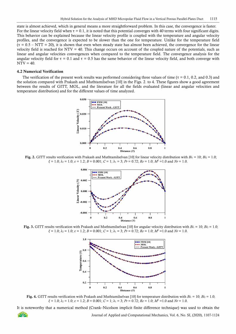
4.2 Numerical Verification
The verification of the present work results was performed considering three values of time (τ = 0.1, 0.2, and 0.3) and the solution compared with Prakash and Muthtamilselvan [10] in the Figs. 2. to 4. These figures show a good agreement between the results of GITT, MOL, and the literature for all the fields evaluated (linear and angular velocities and temperature distribution) and for the different values of time analyzed.
Fig. 2. GITT results verification with Prakash and Muthtamilselvan [10] for linear velocity distribution with Bi1 = 10; Bi2 = 1.0; ξ = 1.0; λ2 = 1.0; ε = 1.2; B = 0.001; C = 1; λ1 = 3; Pr = 0.72; Re = 1.0; M2 =1.0 and Nr = 1.0.
Fig. 3. GITT results verification with Prakash and Muthtamilselvan [10] for angular velocity distribution with Bi1 = 10; Bi2 = 1.0; ξ = 1.0; λ2 = 1.0; ε = 1.2; B = 0.001; C = 1; λ1 = 3; Pr = 0.72; Re = 1.0; M2 =1.0 and Nr = 1.0.
Fig. 4. GITT results verification with Prakash and Muthtamilselvan [10] for temperature distribution with Bi1 = 10; Bi2 = 1.0; ξ = 1.0; λ2 = 1.0; ε = 1.2; B = 0.001; C = 1; λ1 = 3; Pr = 0.72; Re = 1.0; M2 =1.0 and Nr = 1.0.
It is noteworthy that a numerical method (Crank–Nicolson implicit finite difference technique) was used to obtain the
Journal of Applied and Computational Mechanics, Vol. 6, No. SI, (2020), 1107-1124
results from Prakash and Muthtamilselvan [10] (referenced in the figures by FDM [10]), while the results from the method of lines were obtained by using the DIVPAG routine from the IMSL Fortran numerical Library [47] (referenced in the figures by MOL).
4.3 Hydrodynamic Aspects
This section studies the transient behavior as well as the effect of the variation of the system parameters on the linear and angular velocities fields (Figs 5 to 12). The variables and parameters employed in the present analysis were:
- Dimensionless time (τ): which is directly proportional to the dimensional time, t; - Reynolds number (Re): the relation between the inertial forces and the viscous forces; - Hartmann Number (M2): directly proportional to the magnetic field applied externally; - Micropolar Parameter (λ1): directly proportional to the rotational viscosity coefficient; - Dimensionless Thermal Radiation Parameter (Nr): directly proportional to the absorption coefficient.
For the linear velocity, it is possible to observe in Fig. 5 that an increase in the Reynolds number, as expected, increases the velocity distribution in the middle of the channel (accelerate the fluid). Thereby, in the case that Re = 10, inertial forces are more significant than viscous forces. On the other hand, in the condition that Re = 1, both have the same magnitude. It is also observed that there is an increase in suction velocity in the upper plate (positioned at Y = 1) so that the profiles are shifted to the top wall of the channel. Furthermore, the linear velocity profile is increased with time to reach the steady state.
Fig. 5. Transient behavior and effect of Reynolds number on linear velocity distribution with Bi1 = 10; Bi2 = 1.0; ξ = 1.0; λ2 = 1.0; ε = 1.2; B = 0.001; C = 1; λ1 = 3; Pr = 0.72; M2 =1.0 and Nr = 1.0.
Fig. 6. Effect of Hartmann number and Reynolds number on linear velocity distribution with Bi1 = 10; Bi2 = 1.0; ξ = 1.0; λ2 = 1.0; ε = 1.2; B = 0.001; C = 1; λ1 = 3; Pr = 0.72 and Nr = 1.0.
Figure 6 illustrates the effect of the Hartmann number on the stationary linear velocity distribution for Re = 1 and Re = 10. The velocity profiles are parabolic, and there is a maximum value near the middle of the channel, but this maximum is displaced toward Y = 0.6 for large Reynolds number. Also, as M2 is increased, the velocity profile decreases. Hence, the fluid velocity can be reduced by the presence of a strong magnetic field. This behavior can be explained by the Lorentz force, which is a drag-like force produced by the application of a normal magnetic field to an electrically conducting fluid [33], which has an inverse direction to the fluid flow. The effect of Reynolds number (Re) and micropolar parameter (λ1) on the linear velocity profile is examined in Fig. 7. Once again, as expected, the velocity distribution increases as Re is increased by the predominance of inertial forces. On the other hand, it is observed that the velocity profile decreases with an increase in the micropolar parameter. By increasing
Hybrid Solution for the Analysis of MHD Micropolar Fluid Flow in a Vertical Porous Parallel-Plates Duct 1117
Journal of Applied and Computational Mechanics, Vol. 6, No. SI, (2020), 1107-1124
the micropolar parameter, the viscous gyration effects are enhanced, and the fluid flow is damped [36], while the total viscous effect is increased (dynamic viscosity and gyroviscosity) increasing the fluid flow resistance. The velocity profile along the spatial coordinate Y for different values of radiation parameter and the Reynolds number is depicted in Fig. 8. The velocity distribution decreases with an increase in the radiation parameter. Because radiation has a negative contribution to Eq. (5c), the thermal radiation acts as a drain on the energy of the medium and decreases temperature distribution in the fluid, consequently decreasing the velocity magnitude. Additionally, the maximum velocity is near Y = 0.6 in the case of a large Reynolds number (Re = 10). Figure 9 presents the transient response in the angular velocity profile, as well as the effect of the increase on the Reynolds number. The amplitude of the angular velocity profiles grows with time. Between Y = 0.5 and Y = 1 approximately, they are positive, and at about Y = 0 and Y = 0.5, the values of microrotation are negative. Moreover, as the Reynolds number increases the amplitude of the angular velocity is also increased. In the region between Y = 0.0 and Y = 0.5, the fluid is injected, and, as Re is increased, the angular velocity is also increased, on the other hand, between Y = 0.5 and Y = 1.0, the suction effect decreases the angular velocity magnitude.
Fig. 7. Effect of the micropolar parameter and Reynolds number on linear velocity distribution with Bi1 = 10; Bi2 = 1.0; ξ = 1.0;
λ2 = 1.0; ε = 1.2; B = 0.001; C = 1; Pr = 0.72; M2 =1.0 and Nr = 1.0.
Fig. 8. Effect of radiation parameter and Reynolds number on linear velocity distribution with Bi1 = 10; Bi2 = 1.0; ξ = 1.0; λ2 = 1.0;
ε = 1.2; B = 0.001; C = 1; λ1 = 3; Pr = 0.72 and M2 =1.0.
Fig. 9. Transient behavior and effect of Reynolds number on angular velocity distribution with Bi1 = 10; Bi2 = 1.0; ξ = 1.0; λ2 = 1.0;
ε = 1.2; B = 0.001; C = 1; λ1 = 3; Pr = 0.72; M2 =1.0 and Nr = 1.0.
The influence of the Reynolds number as well as the Hartmann number on the angular velocity field is shown in Fig. 10. Observes an increase in the Hartmann number is to increase the angular velocity amplitude between Y = 0 and Y = 0.5
Journal of Applied and Computational Mechanics, Vol. 6, No. SI, (2020), 1107-1124
while decreasing it in between Y = 0.5 and Y = 1. It is noteworthy that this behavior is moved to Y = 1 for higher Reynolds numbers. As the Hartman number is increased, the linear velocity is decreased by the Lorentz forces, decreasing the velocity gradients which increases the angular velocity (according to -λ1∂U/∂Y on Eq. (5b)).
Fig. 10. Effect of Hartmann and Reynolds numbers on angular velocity distribution with Bi1 = 10; Bi2 = 1.0; ξ = 1.0; λ2 = 1.0; ε = 1.2; B = 0.001; C = 1; λ1 = 3; Pr = 0.72 and Nr = 1.0.
Fig. 11. Effect of micropolar parameter and Reynolds number on angular velocity distribution with Bi1 = 10; Bi2 = 1.0; ξ = 1.0; λ2 = 1.0; ε = 1.2; B = 0.001; C = 1; Pr = 0.72; M2 =1.0 and Nr = 1.0.
Fig. 12. Effect of radiation parameter and Reynolds number on angular velocity distribution with Bi1 = 10; Bi2 = 1.0; ξ = 1.0; λ2 = 1.0; ε = 1.2; B = 0.001; C = 1; λ1 = 3; Pr = 0.72 and M2 =1.0.
The angular velocity field for different values of the micropolar parameter and Reynolds number is illustrated in Fig. 11. Unlike the velocity, the angular velocity amplitude increases with the increase of the micropolar parameter. Larger values of the micropolar parameter increase the momentum transfer layer-by-layer because of particle micro-rotation by the escalation of viscosity [36], decreasing the velocity. As the velocity gradient is decreased, the term -λ1∂U/∂Y has less contribution to the amplitude of the angular velocity field; however, the term 2λ1N, which has a positive contribution, slightly increases the magnitude of N. Figure 12 portrays the effect of the radiation parameter as well as the Reynolds number on the angular velocity profile. Increasing the Reynold number increases the inertial forces, which decreases the linear velocity gradients and increases the angular velocity amplitude. The increase of the radiation parameter increases the amplitude of the angular velocity. Higher values of radiation parameter result in the decrease of the temperature, which implies less contribution of body forces (natural convection) in the field of linear velocity. Again, the decrease in the velocity gradients increases the angular velocity.
Hybrid Solution for the Analysis of MHD Micropolar Fluid Flow in a Vertical Porous Parallel-Plates Duct 1119
Journal of Applied and Computational Mechanics, Vol. 6, No. SI, (2020), 1107-1124
Table 3. Shear and couple stresses along the plates (τ = 0.2; Nr = 1.0; Pr = 0.72).
Fig. 13. Transient behavior and effect of Reynolds number on temperature distribution with Bi1 = 10; Bi2 = 1.0; ξ = 1.0; λ2 = 1.0; ε = 1.2; B = 0.001; C = 1; λ1 = 3; Pr = 0.72; M2 =1.0 and Nr = 1.0.
Fig. 14. Effect of radiation parameter and Reynolds number on temperature distribution with Bi1 = 10; Bi2 = 1.0; ξ = 1.0; λ2 = 1.0; ε = 1.2; B = 0.001; C = 1; λ1 = 3; Pr = 0.72 and M2 =1.0.
The shear and the coupled shear stresses over the plates can be observed in Tab. 3. Table 3 demonstrates that an increase in the magnetic parameter will decrease the shearing rates magnitude for both walls. The Lorentz forces induced by the application of the magnetic field decrease the inertial and the micro rotational motion resulting in the reduction of the shear stresses. Instead, by increasing, the Reynolds number enhances the inertial forces, which increase the shearing rates magnitude.
4.3 Heat transfer Aspects
Here we investigate the transient behavior as well as the effect of the variation of the system parameters on the temperature field (Figs. 13 to 16). The variables and parameters employed in the present analysis were:
- Dimensionless time (τ); - Reynolds number (Re); - Dimensionless Thermal Radiation Parameter (Nr); - Type of Heating (Bi1 and Bi2): is a dimensionless quantity used in heat transfer, being the ratio of the heat transfer
Journal of Applied and Computational Mechanics, Vol. 6, No. SI, (2020), 1107-1124
resistances inside and at the surface of a body (Eq. 3k e 3l); - Prandtl number (Pr): describes the relative thickness of the velocity and the thermal boundary layers. It is the relation
between the viscous diffusion and the heat diffusion rates (Eq. (3f)).
The development of temperature distribution with time along the spatial coordinate Y is presented in Figure 13. Keeping the values of the Reynolds number fixed, it is observed that the temperature increases with time. Furthermore, the influence of the Reynolds number is to increase fluid temperature. Therefore, the higher the Reynolds number, the greater the convective heat transfer, and the higher the temperature. Figure 14 illustrates the influence of the radiation parameter, Nr, and Reynolds number on the temperature distribution. The temperature is decreased due to the absorption of energy from the fluid [10] as the radiation parameter is increased. As previously discussed, the radiation term acts as an energy drain in Eq. (5c), and as it increases, the temperature magnitude decreases. The increase of Re increases the inertial forces and the connective transfer, improving the heat transfer and elevating the temperature. In Fig. 15, it is possible to evaluate the influence of the convection heat flux at the walls and the radiation parameter, Nr, on the temperature field. As expected, the increase in thermal radiation leads to a decrease in fluid temperature, as shown in Fig. 14. It is further demonstrated that the highest temperature is associated with the convective flux applied on the wall, with a higher convective flux, the heat transfer is enhanced, and the temperature increased. Because ε = 1.2, the temperature profile is higher at the wall in Y = 1 when Bi2 = 10, than in Y = 0 when Bi1 = 10.
Fig. 15. Effect of radiation parameter and type of heating on temperature distribution with Re = 2; ξ = 1.0; λ2 = 1.0; ε = 1.2; B = 0.001; C = 1; λ1 = 3; Pr = 0.72 and M2 =1.0.
Fig. 16. Effect of Prandtl number and type of heating on temperature distribution with Re = 2; ξ = 1.0; λ2 = 1.0; ε = 1.2; B = 0.001; C = 1; λ1 = 3; M2 =1.0 and Nr = 1.0.
Figure 16 is presented to analyze the effect of the Prandtl number on the temperature field. It is noted that an increase in the Prandtl number decreases the temperature for both studied values of Bi1 and Bi2. A low Prandtl number means that the thermal diffusion rate is higher than the viscous diffusion rate. As Pr increases, the viscous diffusion increases, and the temperature field development is damped, resulting in the decreasing of the temperature profile. Table 4 demonstrates that despite all case studies, the increase in the radiation parameter increases temperature gradient magnitude. A high augmentation of the local heat flux is not observed. Moreover, the effect of radiation is to absorb the heat from the right wall and transfer it to the left wall, whereas the opposite effect is observed for the case of heat flux applied to the right wall [10]. Furthermore, as the Pr number increases, the heat flux is increased mainly in the plate where Bi = 10, which can be explained by the increase of the viscous diffusion rate (high Pr number) associated with the increase in the convective heat transfer (higher Bi number).
Hybrid Solution for the Analysis of MHD Micropolar Fluid Flow in a Vertical Porous Parallel-Plates Duct 1121
Journal of Applied and Computational Mechanics, Vol. 6, No. SI, (2020), 1107-1124
Table 4. Local heat flux along the plates (τ = 0.2; M2 = 1.0; λ1 = 3.0).
The present work evaluates the fully developed transient flow of micropolar fluid between two infinite vertical plates in the presence of a transverse magnetic field by applying the GITT approach. Convergence analysis showed that the temperature field has a more accelerated convergence than the other fields because itis decoupled from the linear and angular velocities. The verification of results obtained with GITT approach performed in comparison with those of the literature and those obtained using the MOL approach were considered satisfactory, so that the computer code developed can be employed for in-depth investigation of the cases evaluated here and further on the effects and conditions over the flow and heat transfer in the channel. The study of the hydrodynamic and heat transfer aspects shows that the increase of the Hartman number decreases the velocity magnitude because of the Lorentz forces, which actuate contrary to the flux direction. The velocity is also decreased by the increase in the micropolar parameter due to the intensification of gryoviscosity. The temperature is decreased by the increase of the radiation parameter and Prandtl number by the absorption of temperature from the fluid and by the viscous diffusion enhancement, respectively. It is noteworthy that no previous studies are employing the solution of micropolar fluid MHD flow in parallel plate channels by the GITT approach. Hence, the present work represents an expansion of the application of the GITT.
Author Contributions
H.K. Miyagawa planned the scheme, initiated the project, and suggested the solution methodology; I.V. Curcino developed the solution methodology and analyzed the numerical results; F.A. Pontes performed the numerical simulation and examined validation for the theory; E.N. Macêdo contributed to demonstrating the physical reasoning behind the results; P.C. Pontes contributed to data analysis; J.N.N. Quaresma conceived the problem and designed the analysis. The manuscript was written through the contribution of all authors. All authors discussed the results, reviewed, and approved the final version of the manuscript.
Acknowledgments
The author (João N.N. Quaresma) would like to acknowledge the financial support provided by the Brazilian sponsoring agency CNPq. The authors also would like to express their gratitude for the valuable suggestions offered by the anonymous reviewers.
Conflict of Interest
The authors declare no potential conflicts of interest with respect to the research, authorship, and publication of this article.
Funding
The authors received no financial support for the research, authorship, and publication of this article.
Nomenclature
Aij Integral transform coefficient (Eq. (25a)) Greek Letters B Micropolar material constant α Thermal diffusivity
Bi1,Bi2 Biot numbers at the left and right walls, respectively β Thermal expansion coefficient C Micropolar material constant (Eq. (7k)) γ Material constant Cij Coefficient of integral transform (Eq. (25a)) γ0 Constant of proportionality Cp Specific heat Γi(y) Velocity fields eigenfunction (Eq. (18a))
Journal of Applied and Computational Mechanics, Vol. 6, No. SI, (2020), 1107-1124
Di Coefficient of integral transform (Eq. (25b)) ( )i yΓ% Normalized velocity fields eigenfunction (Eq. (21))
Eij Coefficient of integral transform (Eq. (25c)) Δy Step size eλ,p Planck’s function ε Dimensionless heat parameter g Acceleration of gravity θ(y,t) Dimensionless temperature (Eq. (7d))
Gij Coefficient of integral transform (Eq. (25a)) θh(y,t) Dimensionless homogeneous solution for temperature (Eq. (8))
Gr Grashof number θp(y) Dimensionless particular solution for temperature (Eq. (8))
H0 Magnetic field intensity ( )iθ τ Transformed temperature field (Eq. (22e))
h1, h2 External convection coefficient at the left and right walls, respectively
κ Velocity fields eigenvalues (Eq. (18b))
Hij Coefficient of integral transform (Eq. (25d)) λ Wavelength j Dimensionless microinertia per unit mass λ1 Micropolar parameter
k, kw Thermal conductivity of the fluid and walls, respectively λ2 Micropolar material constant K Rotational viscosity coefficient µ Dynamic viscosity of the fluid
Kλh Absorption coefficient µi Temperature field eigenvalue (Eq. (13)) L Thickness of the channel ξ Dimensionless parameter (Eq. (7l)) M Hartman number (Eq. (7g)) ν Kinematic viscosity of the fluid
[1] Eringen, A.C., Theory of micropolar fluids, J. Math. Mech., 16, 1966, 1-16. [2] Modather, M., Rashad, A.M., Chamkha, A.J., An analytical study of MHD heat and mass transfer oscillatory flow of a micropolar fluid over a vertical permeable plate in a porous medium, Turkish J. Eng. Env. Sci., 33, 2009, 13. [3] Shercliff, J.A., A Textbook of Magnetohydrodynamics, Pergamon Press, London, UK, 1965. [4] Davidson, P.A., An Introduction to Magnetohydrodynamics, Cambridge University Press, Cambridge, UK, 2001. [5] Sutton, G.W., Sherman, A., Engineering Magnetohydrodynamics, Dover Publications, New York, USA, 2006. [6] Javeri, V., Laminar heat transfer in a rectangular channel for the temperature boundary condition of the third kind, Int. J. Heat Mass Transfer, 21, 1978, 1029–1034. [7] Cuevas, S., Ramos, E., Heat transfer in an MHD channel flow with boundary conditions of the third kind, Appl. Sci. Res., 48, 1991, 11–13. [8] Zueco J., Eguia P., Lopez-Ochoa, L.M., Collazo, J., Patino D., Unsteady MHD free convection of a micropolar fluid between two parallel porous vertical walls with convection from the ambient, International Communications in Heat and Mass Transfer, 36, 2009, 203–209. [9] Lukisha, A.P., Prisnyakov, V.F., The efficiency of round channels fitted with porous, highly heat-conducting insert in a laminar fluid coolant flow at boundary conditions of the third kind, Int. J. Heat Mass Transfer, 53, 2010, 2469–76. [10] Prakash, D., Muthtamilselvan, M., Effect of radiation on transient MHD flow of micropolar fluid between porous vertical channel with boundary conditions of the third kind, Ain Shams Engineering Journal, 5, 2014, 1277–1286. [11] Eringen, A.C., Theory of thermomicrofluids, J. Math. Anal. Appl., 38, 1972, 480–96. [12] Haque, M.Z., Alam, M.M., Ferdows, M., Postelnicu, A., Micropolar fluid behaviors on steady MHD free convection and mass transfer flow with constant heat and mass fluxes, Joule heating and viscous dissipation, J. King Saud Univ. Eng.
Hybrid Solution for the Analysis of MHD Micropolar Fluid Flow in a Vertical Porous Parallel-Plates Duct 1123
Journal of Applied and Computational Mechanics, Vol. 6, No. SI, (2020), 1107-1124
Sci., 24, 2012, 71–84. [13] Babu, M.S., Kumar, J.G., Reddy, T.S., Mass transfer effects on unsteady MHD convection flow of micropolar fluid past a vertical moving porous plate through porous medium with viscous dissipation, Int. J. Appl. Math. Mech., 9(6), 2013, 48–67. [14] Gupta, D., Kumar, L., Singh, B., Finite element solution of unsteady mixed convection flow of micropolar fluid over a porous shrinking sheet, Scientific World Journal, 2014, 11. [15] Ariman, T., Turk, M.A., Sylvester, N.D., Microcontinuum fluid mechanics: a review, Int. J. Eng. Sci., 11, 1973, 905–30. [16] Ariman, T., Turk, M.A., Sylvester, N.D., Microcontinuum fluid mechanics: a review, Int. J. Eng. Sci., 12, 1974, 273–93. [17] Lukaszewicz, G., Micropolar fluids: theory and application, Basel, Birkhauser; 1999. [18] Eringen, A.C., Microcontinum field theory II: Fluent media, New York, Springer; 2001. [19] Sheikholeslami, M., Hatami, M., Ganji, D.D., Micropolar fluid flow and heat transfer in a permeable channel using analytical method, J. Mol. Liq., 194, 2014, 30–6. [20] Umavathi, J.C., Sultana, J., Mixed convective flow of a micropolar fluid mixture in a vertical channel with boundary conditions of the third kind, J. Eng. Phys. Thermophys., 85, 2012, 895–908. [21] Gibanov, N.S., Sheremet, M.A., Pop, I., Free convection in a trapezoidal cavity filled with a micropolar fluid, International Journal of Heat and Mass Transfer, 99, 2016, 831–838. [22] Gibanov, N. S., Sheremet, M.A., Pop, I, Natural convection of micropolar fluid in a wavy differentially heated cavity, Journal of Molecular Liquids, 221, 2016, 518–525. [23] Sheremet, M.A., Pop, I., Ishak, A., Time-dependent natural convection of micropolar fluid in a wavy triangular cavity, International Journal of Heat and Mass Transfer, 105, 2017, 610–622. [24] Miroshnichenko, I.V., Sheremet, M.A., Pop, I., Ishak, A., Convective heat transfer of micropolar fluid in a horizontal wavy channel under the local heating, International Journal of Mechanical Sciences,128-129, 2017, 541–549. [25] Soundalgekar, V.M., Free convection effects on the stokes problem for an infinite vertical plate, ASME J. Heat Transfer, 99, 1977, 499–501. [26] Abo-Eldahab, E.M., Ghonaim, A.F., Radiation effect on heat transfer of a micropolar fluid through a porous medium, Appl. Math. Comput., 169, 2005, 500–10. [27] Rahman, A.M., Sultan, T., Radiative heat transfer flow of micropolar fluid with variable heat flux in a porous medium, Nonlinear Anal.: Model. Contr., 13, 2008, 71–87. [28] Mohamed, R.A., Abo-Dahab, S.M., Influence of chemical reaction and thermal radiation on the heat and mass transfer in MHD micropolar flow over a vertical moving porous plate in a porous medium with heat generation, Int. J. Therm. Sci., 48, 2009, 1–14. [29] Satya Narayana, P.V., Venkateswarlu, B., Venkataramana, S., Effects of hall current and radiation absorption on MHD micropolar fluid in a rotating system, Ain Shams Eng. J., 4, 2013, 843–54. [30] El-Hakiem, M.A., MHD oscillatory flow on free convection radiation through a porous medium with constant suction velocity, J. Magn. Magn. Mater., 220, 2000, 271–276. [31] Srinivasacharya, D., Ramana Murthy, J.V., Venugopalan, D., Unsteady stokes flow of micropolar fluid between two parallel porous plates, Int. J. Eng. Sci., 39, 2001, 1557–63. [32] Bhargara, R., Kumar, L., Takhar, H.S., Numerical solution of free convection MHD micropolar fluid flow between two parallel porous vertical plates, Int. J. Eng. Sci., 41, 2003, 123–36. [33] Ramya, E., Muthtamilselvan, M., Doh, D.H. Absorbing/emitting radiation and slanted hydromagnetic effects on micropolar liquid containing gyrostatic microorganisms, Applied Mathematics and Computation, 324, 2018, 69–81. [34] Lu, D., Ramzan, M., Ahmad, S., Chung, J.D., Farooq, U., A numerical treatment of MHD radiative flow of Micropolar nanofluid with homogeneous heterogeneous reactions past a nonlinear stretched surface, Scientific Reports, 8, 2018, 12431. [35] Doha, D.-H., Choa, G.-R., Ramyab, E., Muthtamilselvanb, M. Cattaneo-Christov heat flux model for inclined MHD micropolar fluid flow past a non-linearly stretchable rotating disk, Case Studies in Thermal Engineering, 14, 2019, 100496. [36] Periyadurai, K., Muthtamilselvan, M., Doh, D.-H. Impact of Magnetic Field on Convective Flow of a Micropolar Fluid with two Parallel Heat Sources, J. Appl. Comput. Mech., 5(4), 2019, 652-666. [37] Kumar, K.A., Sugunamma, V., Sandeep, N., Mustafa, M.T., Simultaneous solutions for first order and second order slips on micropolar fluid flow across a convective surface in the presence of Lorentz force and variable heat source/sink, Scientific Reports, 9, 2019, 14706. [38] Cotta, R.M., Integral Transform in Computational Heat and Fluid Flow, CRC Press, Boca Raton, USA, 1993. [39] Cotta, R.M., Mikhailov, M.D., Heat conduction: lumped analysis, Integral transforms, Symbolic Computation, John Wiley & Sons, Chichester, England, 1997. [40] Pontes, F.A., Macêdo, E.N., Batista, C.S., Lima, J.A., Quaresma, J.N.N., Hybrid Solutions by Integral Transforms for Magnetohydrodynamic Flow with Heat Transfer in Parallel-Plate Channels, International Journal of Numerical Methods For Heat & Fluid Flow, 28(7), 2018, 1474-1505. [41] Lima, J.A., Quaresma, J.N.N., Macêdo, E.N., Integral transform analysis of MHD flow and heat transfer in parallel-plates channels, International Communications in Heat and Mass Transfer, 34, 2007, 420–431.
Journal of Applied and Computational Mechanics, Vol. 6, No. SI, (2020), 1107-1124
[42] Lima, J.A., Rêgo, M.G.O., On the integral transform solution of low-magnetic MHD flow and heat transfer in the entrance region of a channel, International Journal of Non-Linear Mechanics, 50, 2013, 25-39. [43] Pontes, F.A., Miyagawa, H.K., Curcino, I.V., Pontes, P.C., Macêdo, E.N., Quaresma, J.N.N., Integral transform solution of micropolar magnetohydrodynamic oscillatory flow with heat and mass transfer over a plate in a porous medium subjected to chemical reactions, Journal of King Saud University – Science, 37(1), 2019, 114-126. [44] Cogley, A.C., Vincent, W.G., Gilles, S.E. Differential approximation for radiative transfer in a non-gray gas near equilibrium, AIAA Journal, 6, 1968, 551-553. [45] MATHEMATICA, S. Wolfram, A System for doing Mathematics by Computer, Addison Wesley, Reading, MA, 2005. [46] Özisik, M.N., Heat Conduction, John Wiley & Sons, New York, 1993. [47] IMSL, 2010. IMSL Fortran Numerical Library User’s Guide. Visual Numerics, Houston, USA. 1975 p. [48] Schiesser, W.E., Griffiths, G.W., A compendium of partial differential equation models: method of lines analysis with Matlab, Cambridge University Press, New York, 2009.
ORCID iD
Helder K. Miyagawa https://orcid.org/0000-0001-9346-4696 Ingrid V. Curcino https://orcid.org/0000-0002-9925-5542 Fabio A. Pontes https://orcid.org/0000-0002-8442-1317 Emanuel N. Macêdo https://orcid.org/0000-0002-4652-8316 Péricles C. Pontes https://orcid.org/0000-0002-1787-9344 João N. N. Quaresma https://orcid.org/0000-0001-9365-7498
How to cite this article: H.K. Miyagawa, I.V. Curcino, F.A. Pontes, E.N. Macêdo, P.C. Pontes, J.N.N. Quaresma, Hybrid Solution for the Analysis of MHD Micropolar Fluid Flow in a Vertical Porous Parallel-Plates Duct, J. Appl. Comput. Mech., 6(SI), 2020, 1107–1124. https://doi.org/10.22055/JACM.2020.31972.1947


![Second order slip flow of a MHD micropolar fluid over an ......plate was investigated by Nourazar et al. [11] using homotopy perturbation method (HPM). K. Lakshmi Narayana and K. Gangadhar](https://static.documents.pub/doc/80x56/5f96679078ec7462c72a4e7c/second-order-slip-flow-of-a-mhd-micropolar-fluid-over-an-plate-was-investigated.jpg)


![Analysis of Entropy Generation of MHD Micropolar Fluid ... · at different temperatures, (HAM) has been used to solve the problem. H. Ismail et al. [27,28] studied numerically the](https://static.documents.pub/doc/80x56/5f0b0cb27e708231d42e99e3/analysis-of-entropy-generation-of-mhd-micropolar-fluid-at-different-temperatures.jpg)


