Circular pipe is the usual means moving gas or vapor in process plants, utility systems, or pipelines. We will, therefore, emphasize here the design of piping system for gas or vapor of constant viscosity flowing through circular pipes or tubes.
Density of the Flowing Gas or Vapor
As opposed to a liquid which is considered incompressible in a pipe flow hydraulic analysis, a gas or vapor contracts or expands more pronouncedly upon change in pressure. Thus, while the density is fairly constant over a practical range of pressures in a liquid pipe flow system, the density of a gas or vapor, and
consequently its flowing velocity, changes when it flows along the pipe. The term ‘compressible’ is used to describe the gas or vapor fluid flow. It is therefore prudent to consider the effect change in gas density as an improvement of accuracy over the incompressible hydraulic equation for gas or vapor. Density of a gas or vapor is directly a function of temperature and pressure at any given point in the pipe.
To estimate the gas density at the flowing T T and P, an “equation of state”, which governs the pressure-density-temperature relationship is therefore needed.
Ideal Gas Behavior For example, an equation of state for an ideal gas, which is followed closely by many gases of low molecular weight and/or at lower pressures, can be used to calculate the flowing density:
gas idealan for )7.459T)(R(
))(P(M
deg10.73
W
/
F
psia
CFlb (1)
where
WM = molecular weight for the flowing gas, lb/lbmol
Real Gas Behavior At higher pressures, the ideal gas density equation Eq (1) normally is not adequate. To account
for this non-ideality behavior, a third parameter, compressibility factor z , is commonly added to account for the departure from the ideal gas behavior:
gas real afor )7.459T)()(R(
))(P(M
deg73.10
W
/
F
psia
CFlbz
(2)
The compressibility factor z typically approaches 1.0 at lower pressure for real gases (i.e., a real gas behaves more like an ideal gas at lower pressures).
The gas specific gravity gS frequently appears in the hydraulic equations and is defined below:
28.9
Gas of M
Air of M
Gas of MS W
W
Wg (3)
Mass Balance Even through the flowing density of the gas would change along the pipe, the mass flow rate in a piping system will not change unless addition or diversion of flow occurs between two flow locations (Location 1 and Location 2 in the above sketch). This can be demonstrated by Eq (3):
2sec/
22/1sec/11// 22 AAW ftftCFlbftftCFlbhrlb (4)
where W =flow rate in pounds per hour, lb/hr
= flowing density, pounds per cubic foot, lb/CF;
2Aft
= pipe cross-sectional area in square feet, 2ft
2
12
d
4A 2
inch
ft
for a circular pipe. (5)
d = inside diameter of the pipe, inches. = flowing velocity in pipe in feet per second, fps.
scfmq = volumetric flow rate in standard cubic feet per minute (@14.7 psia & 60oF)
scfhq = volumetric flow rate in standard cubic feet per hour (@14.7 psia & 60oF)
MMscfdQ = volumetric flow rate in million standard cubic feet per day (@14.7 psia & 60oF)
Thus, even through the cross-sectional areas of the pipe at Location 2 (downstream) and Location 1 (upstream) are the same, the velocity at Location 2 will be changed from that at Location 1 simply because of the change in pressures due to frictional pressure drop between those two locations. Now we want to introduce two useful parameters associated with the compressible fluid that will appear
later in the pressure drop calculation methods, the sonic velocity s and the Mach number M .
Sonic (or Critical) Velocity in Pipe For compressible fluids, the flowing fluid’s pressure drop will cause the pipe downstream velocity to increase. The maximum possible velocity that flow can attain in a pipe is the velocity of sound in that fluid:
)M(
)T)(z)(k()223(
)M(
)T)(z)(k)(R)(144)(g(
WW
10.73c Ro
Ro
s (7)
where
occurs velocity sonic heat which t fluid of etemperaturT R
o .
A sufficiently high upstream pressure or a sufficiently low downstream pressure can cause the sonic velocity to occur in the outlet end of a pipe or in the downstream of an expanded area. Note also that the sonic velocity will be developed in a pipe line even before its exit if the line is sufficiently long under the above conditions. In this situation, the pressure somewhere in the pipe line at which the sonic velocity occurs can be higher than that at the exit of the pipe line; and the remaining “surplus” pressure drop (from sonic pressure to the exit pressure) will not further increase the flow rate but, in stead, will be consumed in the turbulence of eddies.
Mach number Mach number is defined as ratio of velocity of fluid to velocity of sound in that fluid:
)(k)(M
)(z)(T
)d)((P
W
408
1
)(k)(M
)(z)(T
)D)((P
W10x702.1
)(k)(M
)(z)(T
)A)((P
W0.00001336=
)(k)(M
)(z)(T
)A)((P
W
)223)(3600(
)(RM Number Mach
W
R
2
inchpsia
lb/hr
W
R
2
ftpsia
lb/hr5
W
R
ftpsia
lb/hr
W
R
ftpsia
lb/hr73.10
o
o
o
2
o
2
s
(8)
Critical velocity (or sonic velocity) is defined as the velocity at the point where Mach number reaches unity.
Maximum Capacity of Pipe The maximum mass flow rate that can flow through a pipe line will be limited by the sonic pressure if it is developed before or at the exit of the pipe where the fluid’s flowing velocity at the sonic pressure reaches the sonic velocity of the flowing fluid. To express this maximum mass flow rate, we can use the above
Mach Number equation Eq (8) and set psiaP to psia,cfP and the Mach number to 1.0. Rearrange it to
obtain the maximum flow rate cf,W in a pipe or pipeline as a function of the sonic pressure psia,cfP :
)(z)(T
)(k)(MP
0001336.0
1
)A(
W
)(z)(T
)(k)(MP
)(R
)3600)(232(
)A(
W
R
W,cf
ft
lb/hr cf,
R
W,cf
73.10ft
lb/hr cf,
o2
o2
psia
psia
(9)
)(z)(T
)(k)(MP)408(
)d(
W
)(z)(T
)(k)(M)P(1.702x10
)D(
W
R
W,cf2
inch
lb/hr cf,
R
W,cf
5-
2
ft
lb/hr cf,
o
o
psia
psia
For an ideal-gas isothermal flow segment of constant inside diameter, the material balance equation Eq (4) and Equation of State Eq (1) lead to the following relationship for the Mach number at entrance and exit:
How to detect if sonic velocity will occur in a pipe before its exit?
At any given flow rate lb/hr
W in a pipe of ID = nchid , the critical flow will occur when
the pressure anywhere in pipe deceases to psia cfP or the Mach number increases
to 1.0 before the pipe exit. Thus we can use one of the following, by setting
1M2 in Eq (8), to detect whether lb/hr
W will cause sonic flow:
P )(k)(M
)(z)(T
)A(
W0.00001336
P )(k)(M
)(z)(T
)A(
W
)223)(3600(
)(R
Exit @
W
R
ft
lb/hr
Exit @
W
R
ft
lb/hr73.10
o
2
o
2
(11)
P )(k)(M
)(z)(T
)d(
W
408
1
P )(k)(M
)(z)(T
)D(
W10702.1
Exit @
W
R
2
in
lb/hr
Exit @
W
R
2
ft
lb/hr 5
o
o
x
As will be show in the later sections of this course, at the sonic condition the frictional pressure drop across the pipe can be calculated by the rational formula:
psia avg,
2
1
2
psia 1,
2
psia 2,
psia 1,
ft
ftpsia cf,psia upstream,psi f,
P2
kMP
P
Pln
D
LPPP
i
iKf
where 2
PPP
,2,1
,avg
psiapsia
psia
;
or by the modified Darcy's equation
)(144))(g2(
))((
Y
1
D
LPPP
c
2
2cfupstream
fK
i
if
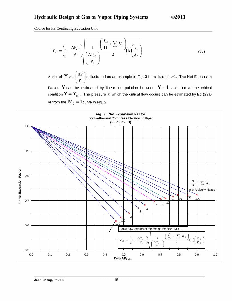
where Y= net expansion factor. All parameters are evaluated at the upstream conditions.
Any pressure lower than Pcf (i.e., from Pcf to P Exit @ ) will be lost in shock
waves and turbulence instead of being converted into useful kinetic energy. In other words, if the pipe outlet is exposed to another environment which has a pressure that is lower than the calculated Pcf , the pressure at the outlet end of pipe will be Pcf ; and the remaining pressure drop (from Pcf to the pressure in the downstream environment) will be wasted.
Overall Pressure Balance The overall pressure balance equation for each flow segment of constant inside diameter flowing an incompressible fluid is
accfps PPPP+P (12)
or accfp
outin
outin PPP144
h))((
144
h))((+P-P
where
inP = pressure at the inlet of the segment, psig
outP = pressure at the outlet of the segment, psig
ΔP = system total pressure drop = inP - outP , psi
sΔP = segment static pressure change due to change in elevation , psi
out
/
in
/
s144
)h)((
144
)h)((P
ftCFlbftCFlb
psi
pΔP = pressure increase due to compressor, psi
fΔP = segment frictional pressure drop, psi
accΔP = segment pressure drop due to fluid acceleration, psi
= flowing density, pounds per cubic foot, lb/CF;
h = elevation, ft
Acceleration pressure drop, accΔP , can be appreciable for a compressible flow when the pressure drop
and the increase in flowing velocity is substantial. As will be shown later in this course, the calculation of frictional pressure drop of compressible flow will include the effect of acceleration. Furthermore, we will
not address the compressor flow in this study guide. Consequently, 0ΔPp .
The overall pressure balance equation for a gas flowing through a series of pipes becomes:
f
downflow
outin
upflow
outinoutin P
144
)h-h(
144
)h-h(+ P- P
outinoutin
(13)
While Eq (13) is useful for an isothermal flow system, it is applicable to a flowing system under hydraulic analysis whose flowing temperature undergoes changes such as flowing through an heat exchanger. We
can calculate the fP for each isothermal flow segment and then also sum them up to obtain the
cumulative frictional pressure drop fP for the entire system.
Hydraulic Terminology in Pipe Flow Some frequently used hydraulic terminologies relating to the word “head” (for pressure) are introduced below:
Pressure, Pressure Head Pressure is the force exerted by fluid that acts to pipe or container and can be expressed as force per square unit surface area. This pressure typically can be measured directly by a pressure gage in a unit such as pounds per square inch, psig. Parallel to the principle of a mercury barometer, the same pressure that is exerted by the fluid
also can cause a measuring fluid to rise in a column to a height of ftH until its weight balances
out the pressure in the pipe or container. In other words, a column of liquid will exert a local
Pressure that is proportional to the height of that liquid:
144
)H)((P
/
ftCFlb
psia
(14)
Thus, the pressure in the pipe or container can be expressed by the height of the column of a
measuring gas, such as mercury, water or the same fluid itself, and is called Pressure Head:
CFlb
psia
ft
/
)P)(144(H
(15)
For example, normal atmospheric pressure at 0 psig or 14.6959 psia and 60oF is equivalent to a
head of mercury of 29.92 (=14.69X144/848.7X12) inches or a head of water of 33.93 (=14.6959X144/62.3688) feet. Therefore, the pressure will increase by 2.036 psi per inch of mercury column rise or 0.433 psi per foot of water column height: 14.6959 psi = 29.92“ Hg = 760 mmHg 1 psi = 2.036”Hg 0.433 psi = 1’ WC (60
oF, density = 62.3688 lb/CF)
1 psi = 2.31’ WC (60oF, density = 62.3688 lb/CF)
Static Pressure, Static Head Static head is a measurement of pressure due to the weight of column of fluid at a given height. Thus, a fluid at a level of H feet above a reference point (a difference in elevation) is said to have
a static head of ft s,H . This Static Head of H feet also can be expressed in terms of a local
pressure at the base of the column if the density of the fluid is known, for example,
144
)H)((H
s,/
s,
ftCFlb
psi
in pounds per square inch of area. (16)
Static head psi ,sH also can be called Static Pressure simply because it measures the
pressure head and is expressed in a pressure unit.
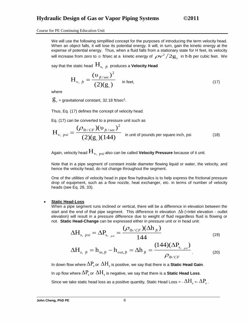
We will use the following simplified concept for the purposes of introducing the term velocity head. When an object falls, it will lose its potential energy. It will, in turn, gain the kinetic energy at the expense of potential energy. Thus, when a fluid falls from a stationary state for H feet, its velocity
will increase from zero to ft/sec at a kinetic energy of c
v 2g2 in ft-lb per cubic feet. We
say that the static head ft s,H produces a Velocity Head
))(g2(
)υ(H
c
2
sec/
v,
ft
ft in feet, (17)
where
cg = gravitational constant, 32.18 ft/sec2.
Thus, Eq. (17) defines the concept of velocity head. Eq. (17) can be converted to a pressure unit such as
)(144))(g2(
)υ)((H
c
2
sec//
v,
ftCFlb
psi
in unit of pounds per square inch, psi (18)
Again, velocity head psi v,H also can be called Velocity Pressure because of it unit.
Note that in a pipe segment of constant inside diameter flowing liquid or water, the velocity, and hence the velocity head, do not change throughout the segment. One of the utilities of velocity head in pipe flow hydraulics is to help express the frictional pressure drop of equipment, such as a flow nozzle, heat exchanger, etc. in terms of number of velocity heads (see Eq. 28, 33).
Static Head-Loss When a pipe segment runs inclined or vertical, there will be a difference in elevation between the
start and the end of that pipe segment. This difference in elevation h (=inlet elevation - outlet elevation) will result in a pressure difference due to weight of fluid regardless fluid is flowing or
not. Static Head-Change can be expressed either in pressure unit or in head unit:
144
)h)((PH
/
s, s,
ftCFlb
psi psi
(19)
CFlb
ftftftft
psi
/
s,
,outin, s,
)P)(144(hhhH
. (20)
In down flow where sΔP or sΔH is positive, we say that there is a Static Head Gain.
In up flow where sΔP or sΔH is negative, we say that there is a Static Head Loss.
Since we take static head loss as a positive quantity, Static Head Loss = - sΔH =- sΔP .
When an overall piping circuit involves several pipe segments which has its own elevation change, these individual elevation changes can be added together to arrive at the overall elevation change. In other words, the static head change is additive and the net static head change for the overall system of constant density depends on only the elevation at the start and the end of that piping circuit.
Dynamic Head-Loss
The term Dynamic Head-Loss or Dynamic Pressure Drop refers to the frictional pressure drop associated with piping (pipe and flow elements) plus equipment:
psipsi f, f, PH (21)
CFlb
ft
psi
/
f,
f,
)P)(144(H
(22)
The formula for psi f,P will be presented later.
Total Head-Loss
Loss Head StaticLoss Head DynamicLoss Head Total (23)
Total head loss is also called System Pressure Drop.
Finally, the overall pressure balance equation, Eq. 12, for a compressible fluid, such as a gas, flowing through a series of pipes can be written in terms of heads:
ftCFlb
psi
fftfft
ftCFlb
psia
CFlbi
psia
/ avg
f,
downflowt out, in,upflowt out, in,
/out
out,
/n
in, )144)(P(h-hh-h+
)(144) (P -
)(144) (P
Total Head Loss - Static Head Loss Dynamics Head Loss (24)
Reynolds number Re
This is the parameter used to establish the flow regimes in a pipe. The value of friction factor, which is used to correlate the dynamics head loss, depends on the Reynolds number
Reynolds number Flow Regime < 2,000 Laminar 2,000 to 4,000 Transition > 4,000 Turbulent
D = inside diameter of the pipe, ft To calculate the Reynolds number, all parameters, i.e., , , and , related to the fluid shall be
evaluated at the flowing temperature and pressure, converting from standard condition such as 60oF and
1 atmosphere to the flowing conditions. Most fluid flowing in the in-plant piping or pipelines are in the turbulent flow regime.
Friction Factor f
Darcy friction factor is more commonly used in the engineering calculations.
For laminar flow: f 64
Re. (26)
For turbulent flow, Moody’s chart is generally accepted for the friction factor calculation. The Colebrook-White equation is an analytical form for the Moody’s friction factor:
12
3 7
2 5110
f f log [
.
.
Re]
d (27)
The Cole Brook-White equation representation of Moody’s friction factor is plotted in Fig. 1.
For turbulent flow, Moody’s friction is correlated with both Reynolds number and the pipe’s absolute roughness. Typical values are listed below for new pipes:
Table 1
Recommended Absolute Roughness
Pipe or Tubing Material feet inches
Drawn Tubing 0.000 005 1 0.000 06
Teflon, PTFE; PFA-PTFE 0.000 005 0.000 06
High Density Polyethylene, PVDF; PVC; etc 0.000 07 0.000 84
Absolute roughness can increase over time after initial service, resulting in higher frictional pressure drop. For example, it can double in 10 to 15 years for petroleum residues and in 25 to 35 years for light distillates. Whenever possible, a back calculated absolute roughness from actual pipe pressure drop data would be preferred.
Darcy Friction Factor for a commercial pipe at Complete Turbulence(1)
Treat the gas as an ideal gas (i.e., : 1z ) flowing in pipe with changing density along the pipe (which effects the acceleration) to be accounted for by fluid’s isothermal expansion via Eq. (1):
2
2,
,1
2
1,
,2
2
1ft
ft
P
Pln
P
P1
kM
1
D
L
psia
psia
psia
psia
i
iKf
for inlet Mach number 1M (28)
or
2
2,
,1
2
2,
,1
2
2P
Pln1
P
P
kM
1
D
L
psia
psia
psia
psia
i
iKf
for outlet Mach number 2M (28a)
where
i
iK = Summation of Resistance Coefficient or Number of Velocity Heads for equipment,
valves and fittings that are attached in that pipe segment. The graphical form of Eq (28a) are illustrared below for a fluid of k=1:
Eq (28) or (28a) can be re-arranged to express the frictional pressure drop
21f PPP as follows:
psia
psia
psia
psia
i
ipsiapsiapsi Kf
avg,
2
1
2
1,
2
2,
1,
ft
ft 2, 1, f,
P2
kMP
P
Pln
D
LPPP
(30)
psia
psia
psia
psia
i
i
ft
f
psia psiapsi Kf
avg,
2
2
2
2,
2
2,
1,t
2, 1, f,P2
kMP
P
Pln
D
LPPP
(30a)
where 2
PPP
,2,1
,avg
psiapsia
psia
.
To solve for fP or 2P from Eq (30) or (30a), an trial-and-error solution is also needed.
An alternate graphical approach can be used. First, assume a pipe outlet pressure 2P ,
calculate the outlet Mach number 2M and calculate the total velocity head of pipe plus
valves and fittings i
iKf
D
L. Then, read off
1
2
P
P from Fig. 2. Obtain a calculated 2P
(in absolute, psia) by multiplying the inlet pressure 1P (in absolute, psia) to this ratio.
Iterate until the assumed and the calculated 2P agree. Finally,
a 2, 1, f, PPP psipsiapsi .
Long Gas Pipe Line – A Simplified Case from the Rational-Formula For a long pipe line where the friction due to line is more significant than that due to the pipe bends or fittings and the line is sized to optimize the line pressure drop, then
2
2
1
D
L
D
L
P
Pn
fK
f
i
i and Eq (28) can be simplified to become:
2
1,
2
2,
2
1,
2
1ft
ft
P
PP
kM
1
D
L
psia
psiapsiaf (31)
Eq (31) can be re-written in terms of mass or volumetric flow rates:
Eq (31a), (31b) and (31c) are a little akward to use, but can be further simplified to more useful working forms in terms of average line pressure as defined previously:
5
,1
2
/ft
a avg,
1,6
4
,1
2
/
psia avg,
psia 1,
ft
ft
2
psia avg,
2
1
2
psia 1,
ft
ft f,
)d)((
)W(L
P
P10356.3
)d)((
)W(
P
P
D
L
1891
1
P2
kMP
D
LP
inchlb/CF
hrlb
psi
psia
inchlb/CF
hrlb
psi
fx
f
f
(31d)
5
,avg
2
9
f)d)(P(
)q(STL)(10x26.7P
inchpsia
scfhgoft R
psi
zf
(31e)
5
,avg
2
f)d)(P(
)Q(STL)(65.12P
inchpsia
MMscfdgoft R
psi
zf (31f)
Eq (31) and its variations such as (31a), (31b), (31c), (31d), (31e) and (31f) are called
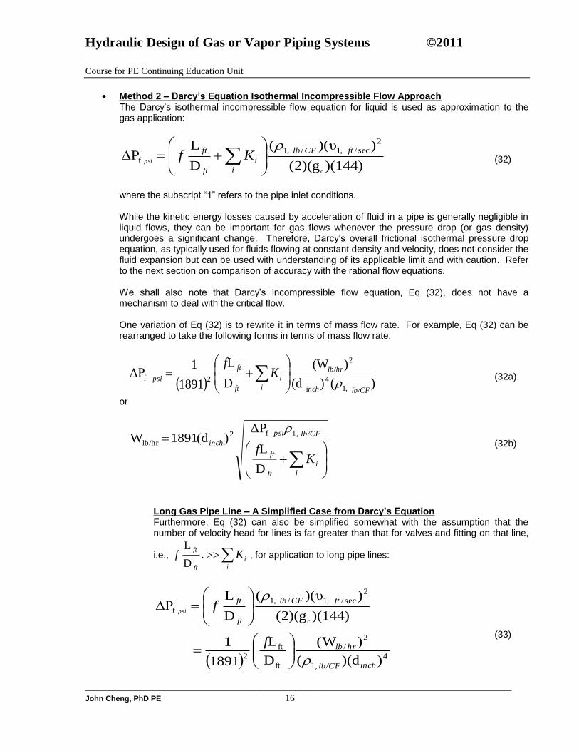
Method 2 – Darcy’s Equation Isothermal Incompressible Flow Approach The Darcy’s isothermal incompressible flow equation for liquid is used as approximation to the gas application:
)(144))(g2(
)υ)((
D
LP
c
2
sec/ ,1/ ,1
f
ftCFlb
i
i
ft
ftKf
psi
(32)
where the subscript “1” refers to the pipe inlet conditions. While the kinetic energy losses caused by acceleration of fluid in a pipe is generally negligible in liquid flows, they can be important for gas flows whenever the pressure drop (or gas density) undergoes a significant change. Therefore, Darcy’s overall frictional isothermal pressure drop equation, as typically used for fluids flowing at constant density and velocity, does not consider the fluid expansion but can be used with understanding of its applicable limit and with caution. Refer to the next section on comparison of accuracy with the rational flow equations. We shall also note that Darcy’s incompressible flow equation, Eq (32), does not have a mechanism to deal with the critical flow. One variation of Eq (32) is to rewrite it in terms of mass flow rate. For example, Eq (32) can be rearranged to take the following forms in terms of mass flow rate:
)()d(
)(W
D
L
1891
1ΔP
,1
4
i
2
2 f
lb/CFnch
lb/hr
i
i
ft
ft
psiK
f
(32a)
or
i
i
ft
ft
, lb/CFpsi
inch
Kf
D
L
ΔP)d(1891W
1 f2
lb/hr
(32b)
Long Gas Pipe Line – A Simplified Case from Darcy’s Equation Furthermore, Eq (32) can also be simplified somewhat with the assumption that the number of velocity head for lines is far greater than that for valves and fitting on that line,
in terms of inlet flowing parameters and standard volumetric flow rate. Notice that all flowing parameters applying to Darcy’s equation are evaluated at the pipe entrance conditions. Potential applicable flow situation using Darcy’s equation is for short piping runs without significant heat transfer to or from pipe.
Method 3 - Darcy’s Isothermal Equation with Net Expansion Factor To account for the effect of gas expansion and acceleration when using Darcy’s frictional pressure drop equation, a correction factor can be incorporated. The correction is achieved by
incorporating an additional parameter, called Net Expansion Factor ( Y ), into Eq (32) using the flowing conditions at pipe inlet:
)(144))(g2(
))((
Y
1
D
LP
c
2
,1/ ,1
f 2
fpsCFlb
i
i
ft
ft
psi Kf
(34)
Similarly, the dynamic head loss can also be expressed in terms of flow rates as follows:
)()d(
)(W
D
L
Y
1
1891
1ΔP
,1
4
i
2
f
22 f
lb/CFnch
lb/hr
i
i
ft
t
psiK
f
(34a)
or
i
i
ft
ft
lb/CFpsi
nchb/hr
Kf
1
,1 f2
il
D
L
ΔP)d)(Y)(1891(W
(34b)
The cfY is obtained by solving Eq. (34) at the sonic conditions
( cf PP , cf YY ) with the help of Eq (1) the density equation, and Eq (4) the
Comparison between the Rational and Darcy’s methods
Let’s now examine if there is any difference in the result of fP calculation by the Darcy-based
incompressible flow approach Eq (33) and the isothermal compressible flow rational formula Eq (31). Both of these two equations are plotted below for an illustration case with the lumped parameter A of 100,
where
5
2
9
)d(
)q(STL)(10x26.7
inch
scfhgoft Rzf
A
300
320
340
360
380
400
420
440
460
480
500
0 200 400 600 800 1000 1200
distance, ft
P2, p
sig
P2 Darcy
P2 Rational
A=100
As expected, the Darcy’s formula calculates a higher outlet pressure (i.e., lower line pressure drop) because the flow density was not allowed to change along the pipe and, hence, no pressure decrease due to gas expansion was accounted. The percent deviation of calculated pressure drop of Darcy’s incompressible formula from the rational formula is illustrated below:
0.00%
5.00%
10.00%
15.00%
20.00%
0.00 0.05 0.10 0.15 0.20 0.25 0.30 0.35 0.40 0.45
deltaP/P1 darcy
(dP
darc
y-d
Pra
tio
n)/
dP
rati
on
As one can see that the deviations become large when the calculated pressure drop by Darcy’s equation is high relative to the pipe entrance pressure. To allow the deviation of the Darcy’s to be below reasonable range, it is recommended that the simpler Darcy’s incompressible equation be used when the following criterion is met:
Total segment frictional pressure drop 10% of the segment entrance pressure.
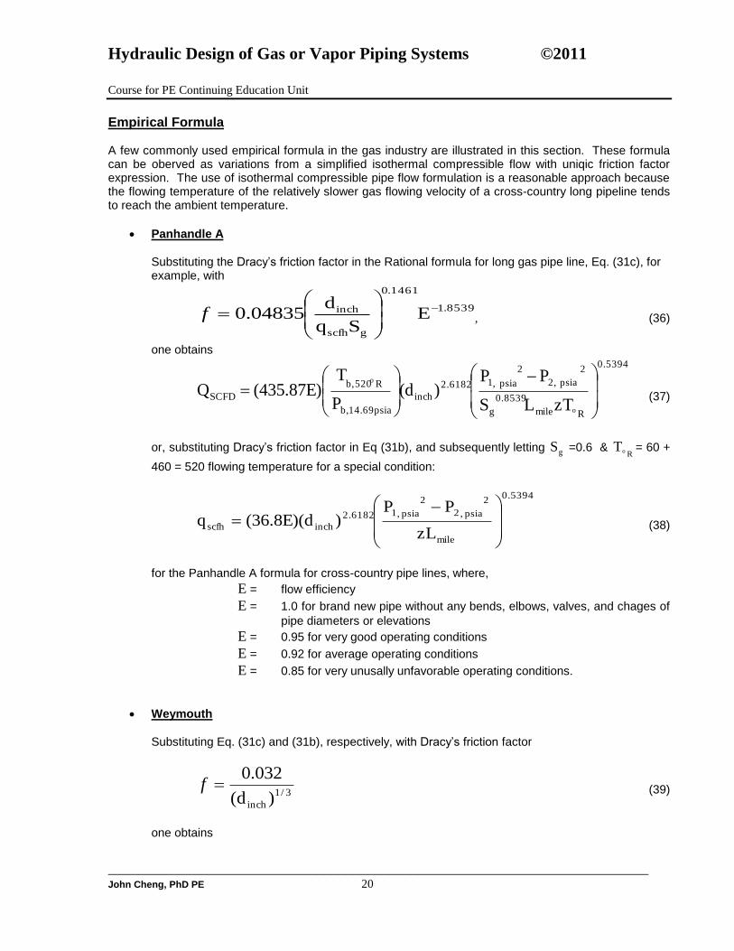
Empirical Formula A few commonly used empirical formula in the gas industry are illustrated in this section. These formula can be oberved as variations from a simplified isothermal compressible flow with uniqic friction factor expression. The use of isothermal compressible pipe flow formulation is a reasonable approach because the flowing temperature of the relatively slower gas flowing velocity of a cross-country long pipeline tends to reach the ambient temperature.
Panhandle A
Substituting the Dracy’s friction factor in the Rational formula for long gas pipe line, Eq. (31c), for example, with
8539.1
1461.0
gscfh
inch ESq
d04835.0
f , (36)
one obtains
zTLS
PP)(d
P
T(435.87E)Q
0.5394
Rmile
0.8539
g
2
psia 2,
2
psia ,12.6182
inch
14.69psia b,
R520 b,
SCFD
o
o
(37)
or, substituting Dracy’s friction factor in Eq (31b), and subsequently letting gS =0.6 & RoT = 60 +
460 = 520 flowing temperature for a special condition:
zL
PP)(36.8E)(dq
0.5394
mile
2
psia ,2
2
psia ,12.6182
inchscfh
(38)
for the Panhandle A formula for cross-country pipe lines, where,
E = flow efficiency
E = 1.0 for brand new pipe without any bends, elbows, valves, and chages of
pipe diameters or elevations
E = 0.95 for very good operating conditions
E = 0.92 for average operating conditions
E = 0.85 for very unusally unfavorable operating conditions.
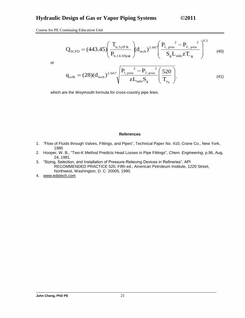
Weymouth
Substituting Eq. (31c) and (31b), respectively, with Dracy’s friction factor
which are the Weymouth formula for cross-country pipe lines.
References
1. "Flow of Fluids through Valves, Fittings, and Pipes", Technical Paper No. 410, Crane Co., New York, 1985
2. Hooper, W. B., "Two-K Method Predicts Head Losses in Pipe Fittings", Chem. Engineering, p.96, Aug. 24, 1981.
3. “Sizing, Selection, and Installation of Pressure-Relieving Devices in Refineries”, API RECOMMENDED PRACTICE 520, Fifth ed., American Petroleum Institute, 1220 Street, Northwest, Washington, D. C. 20005, 1990.