Hydro GeoAnalyst: Getting Started...

Hydro GeoAnalyst: Getting Started TutorialThis tutorial provides instructions on how to “Get Started” quickly with Hydro GeoAnalyst, using your own data sets. There is information on how to create a new Hydro GeoAnalyst project, then enter, manipulate, and visualize the data. You are encouraged to refer to respective chapters in the User’s Manual, for more details on each module.

The tutorial is organized into the following sections:

1.1: Creating a New Project

• Database Environment• Template Settings• Project Settings

1.2: Data Management

• Entering Data Manually• Importing Data Using the Data Transfer System (DTS)• Grouping Stations

1.3: Viewing Borehole Log Plots

• Selecting a Template• Saving and Printing

1.4: Querying the Database

• Creating a data query• Recalling and executing queries

1.5: Mapping the Data

• Creating a Map Project• Importing and GeoReferencing Site Maps• Creating Contour maps• Defining Cross Section Lines

1.6: Interpreting and Viewing Cross-Sections

• Creating Geological Cross Sections• 3D Visualization of Cross Sections

1.7: Preparing Reports

• Creating Reports with Data from Project• Creating Charts

1

Terms and NotationThe following terms and notations will be used in this exercise:

type: Type in the given word or value

Click the left mouse button where indicated

Double-click the left mouse button where indicated

<Tab> Press the Tab key on your keyboard

<Enter> Press the Enter key on your keyboard

The bold faced type indicates menu or window items to click.

The Main Menu items are the items available at the top of the Hydro GeoAnalyst Parent window.

1.1 Creating a New ProjectTo start Hydro GeoAnalyst,

Start and choose Programs > SWS Software> Hydro GeoAnalyst>Hydro GeoAnalyst 2010.1.

When Hydro GeoAnalyst is loaded, there will be no project loaded by default. In order to enter your station data, you either have to open an existing project or create a new one using the Project Wizard. To create a new project, follow through the steps of the Project Wizard as outlined below:

Project > New from the main menu, or click the (New) button from the toolbar.

A prompt will appear for the user name and password, in a dialog as shown in the example below:

HGA includes a default user “Admin” with no password.

You must enter a valid user name and password, for a user that has privileges for creating new projects. HGA will then check these credentials in the security document, to confirm that this user has these privileges. For more details on assigning user access

2 Hydro GeoAnalyst: Getting Started Tutorial

controls, please see the User Access Level Management chapter in your HGA User’s Manual.

If you have modified the default Admin user, or added additional users (with permissions to create projects), then login now with the appropriate credentials.

Click [OK]

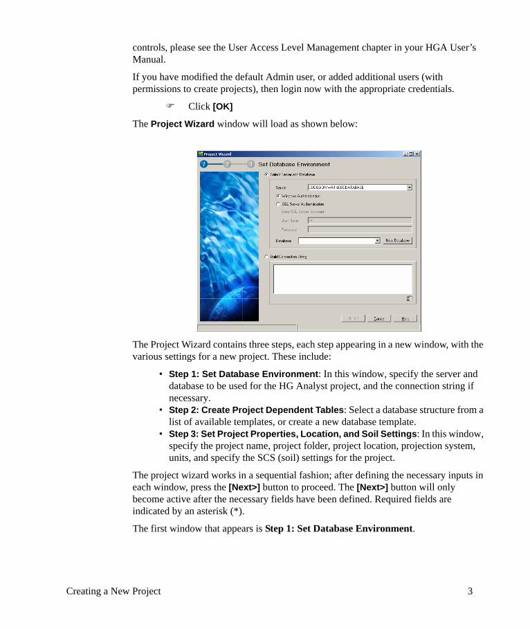
The Project Wizard window will load as shown below:

The Project Wizard contains three steps, each step appearing in a new window, with the various settings for a new project. These include:

• Step 1: Set Database Environment: In this window, specify the server and database to be used for the HG Analyst project, and the connection string if necessary.

• Step 2: Create Project Dependent Tables: Select a database structure from a list of available templates, or create a new database template.

• Step 3: Set Project Properties, Location, and Soil Settings: In this window, specify the project name, project folder, project location, projection system, units, and specify the SCS (soil) settings for the project.

The project wizard works in a sequential fashion; after defining the necessary inputs in each window, press the [Next>] button to proceed. The [Next>] button will only become active after the necessary fields have been defined. Required fields are indicated by an asterisk (*).

The first window that appears is Step 1: Set Database Environment.

Creating a New Project 3

1.1.1 Step 1: Set Database EnvironmentIn the first step, define the server and database settings for the new project. Hydro GeoAnalyst uses Microsoft SQL Server 2005 Express to host the project database. Any MS SQL Express server that is currently installed on any computer on your network could be used as long as you have the appropriate access rights to it. If you are working on a stand-alone computer, then the “server” would be the local computer using SQL Express. Once the server is selected, select from an existing database on this server, or create a new database.

In this example, you will create the project on the local machine.

Select Server and DatabaseChoose the Select Server and Database option.

Beside Server select your local machine as the Server; this will appear as Computer_Name\WHI in the combo box.

If a separate login password is not required for the selected Server computer, be sure to check the box beside Windows NT Integrated Authorization. Otherwise, de-select this option, and specify a User Name and Password. This will allow Hydro GeoAnalyst to automatically log on to the Server each time the project is opened

Note: If you cannot see your local WHI instance of SQL Express when creating a new project, or opening an existing project, please refer to the FAQ section in the User’s Manual for some troubleshooting suggestions.

After the Server is selected, Hydro GeoAnalyst will automatically scan the Server for valid SQL databases. These databases will then appear in the combo box beside Database. You have the options of using an existing Hydro GeoAnalyst database to host your project, or creating a new database on the specified server.

In this example, a NEW database will be created on the local machine:

Beside Database, select Create New Database from the combo box. The following dialog will appear:

type: SampleDatabase

Click [OK].


[Next>] to create the new database, and proceed to the Step 2 in the Project Wizard.

1.1.2 Step 2: Create Project Dependent TablesThe second step in the Project wizard contains the Database Structure settings, which includes the database template for the new project. These options are shown in the figure below:

In this window, select from one of the pre-defined Database templates for the new project. The template contains the necessary tables, fields, relationships, linked lists, and reports for storing and interpreting data in the Hydro GeoAnalyst database. The following templates are available, in both imperial and metric length units:

• Environmental• US EPA Region 2• US EPA Region 5• MOE - WWIS (Ontario Ministry of Environment Water Well Information

System)

[Environmental-metric] template, from the Templates combo box, for this example.

[Next] button to create the project dependent tables for this database.

1.1.3 Step 3: Set Project Properties and LocationThe third step in the Project wizard contains general project information, as seen in the figure below:


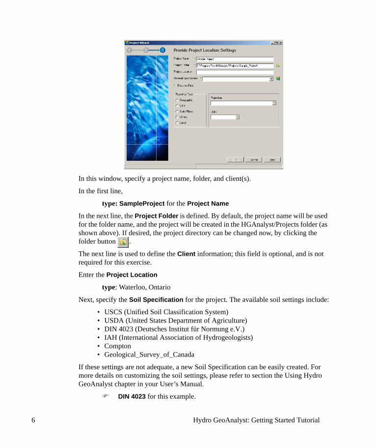
In this window, specify a project name, folder, and client(s).

In the first line,

type: SampleProject for the Project Name

In the next line, the Project Folder is defined. By default, the project name will be used for the folder name, and the project will be created in the HGAnalyst/Projects folder (as shown above). If desired, the project directory can be changed now, by clicking the folder button .

The next line is used to define the Client information; this field is optional, and is not required for this exercise.

Enter the Project Location

type: Waterloo, Ontario

Next, specify the Soil Specification for the project. The available soil settings include:

• USCS (Unified Soil Classification System)• USDA (United States Department of Agriculture)• DIN 4023 (Deutsches Institut für Normung e.V.)• IAH (International Association of Hydrogeologists)• Compton• Geological_Survey_of_Canada

If these settings are not adequate, a new Soil Specification can be easily created. For more details on customizing the soil settings, please refer to section the Using Hydro GeoAnalyst chapter in your User’s Manual.

DIN 4023 for this example.


There is an option to enter a Description of the project location at the bottom of this window (not a required field).

Next, define the Project Location Settings information, such as the projection system and coordinate settings. Under the Projection Type frame, specify the coordinate system used for this project. You may choose from the following list:

• Geographic• UTM• State Planar• Other• Local

For this sample project,

UTM

Once the projection Type is selected, choose the Projection from the combo box on the right side of the window. The Units will be selected automatically, based on the selected projection type (e.g. UTM will use m, State Planer will use feet, etc.)

NAD 1983 UTM Zone 17N

[Finish] to complete the Project Wizard.

The first time the project loads, the settings for User Access Management will be presented. As the creator of the new project, you will have Administrator rights, where you can add/remove users, and assign access rights. For more details on this feature, please see the User Access Management chapter in your User’s Manual.

[X] button in the upper-right corner, to close the User Access Management window.

The new project will then be created, with the necessary tables, fields, and settings. Once this is complete, the main Hydro GeoAnalyst window will appear with the new project, as shown below.


If necessary, the project settings can be modified at any time by selecting Properties from the Project menu.

In addition, the database view and structure can be modified using the Template Manager. For more details, see consult the Template Manager chapter in your User’s Manual.

Now that the new project has been created, the station data may be entered. For instructions on this procedure, please continue to the next section.

1.2 Data ManagementThere are two options for entering data into the new project:

• Manually in the grids; OR• Importing from other sources using the Data Transfer System (DTS)

To facilitate data entry, there are two tabs available in the Hydro GeoAnalyst window, located directly below the main toolbar: Station List and Station Data tab.

• Station List Tab: This tab hosts a grid displaying a list of stations for the selected station group. Here, you can enter the basic location information for the stations: Name, X and Y coordinate, Elevation, and TOC (Top of Casing) elevation.


• Station Data Tab: This tab allows entering and viewing data for an individual station. This tab can be activated either by clicking on a data category node in the Project Browser or by clicking on the tab itself, provided at least one station is already selected. Each table in the selected Data Category will be displayed in a separate tab under the Station Data tab. The data is displayed for the Station selected at the top of the window. To change the active station, simply select a new station from the list above the grid.

Now that you are familiar with the data entry options, a few brief examples are provided below.

1.2.1 Entering Data ManuallyIf there are only a few stations to be entered into the project (or if you have data as a hard copy), then the quickest method may be to manually enter the data for each station. (if you have a large data set in a source file(s), feel free to skip ahead to the section Importing Data using the DTS).

Example: Creating a New Station + beside the Station Groups node in the project browser

Project under the Station Groups node in the project browser

Record > Add from the main menu, or press the (Add) button in the toolbar. A new row will be added to the grid in the Station List tab. Enter the following information for this station:

In the Name column,

type: BH1

<Tab> or <Enter> key on the keyboard, to shift the focus to the next cell.

In the X column,

type: 537381.50

In the Y column,

type: 4812036.33

In the Elevation column,

type: 347

In the TOC column,

type: 348

To post (save) the data for this record,

Data Management 9

Record > Post from the main menu, or press the (Post) button in the toolbar.

Using the same procedure, enter the following information for these new stations:

Name X Y Elev TOC

BH2 535780.7 4813800.1 339.1 340.1

BH3 535111.6 4813600.3 338.1 339.1

BH4 538544.4 4814890.8 350.5 351.5

BH5 533866.3 4811787.2 350.0 351.0

OW1 535915.6 4813215.3 340.5 341.5

As long as you remain in the same window, you do not need to press the Post button after every entry. Do so to finalize the changes you have made before moving to the next window.

Note the color of the fields you have modified is different (yellow); once you press the Post button they return to the default state (white). This feature allows you to easily distinguish between permanent changes, and the recent ones that have not yet been saved to the database.

Once you are finished, remember to save the new data. The stations should now appear in the Station List, similar to the image shown below:


As each station is added to the database, it is assigned a unique station ID value. The station ID for the selected station can be seen in the task bar in the Station List window (an example is circled above for station OW-1, the station ID is 6). The station ID is the primary key; it is required in all source tables during import, so that data can be matched to the appropriate station. If your source tables do not contain station ID’s, you may use the station names, and HGA will map the data to the appropriate station ID.

Next, you will enter additional data for one of the new stations.

BH1 from the Station List, then

Station Data tab.

The Station Data tab provides the interface for viewing/entering detailed data for an individual station. There are several Data Categories available in Hydro GeoAnalyst; Data Categories are provided to enable logical grouping of your tables. A Data Category may be selected from the combo box at the top of the window, or from the Station Data node in the project browser. By default, the Description data category will be displayed, and the Location table will be activated for this station.

Selecting a new Data Category will display all the available tables and fields belonging to the selected category. The following is a summary of the Data Categories included in Hydro GeoAnalyst, along with some of the tables and fields:

Data Category Tables and Fields

Description Station name, world coordinates, elevation, TOC elevation

Geologic Description Soil description (e.g. from split-spoon soil sampling and drilling)

Well Construction Well casing intervals, packing depths, drilling method, etc.

Soil Testing Soil physical properties

Soil Sampling Soil sampling events (chemical analysis)

Monitoring Event Water table elevations or groundwater chemistry data

Mining and Exploration Alteration, Mineralization, Structure, Samples, Down Hole Survey, Down Hole Geophysics

Geophysics Conditions, Gamma, Neutron, 64 in E-log, 16 in E-log, Density

Well History Well installation, owner, permit to take water, decommissioning, etc.

Data Management 11

The example below illustrates how to enter Lithology data in the Geologic Description category, for several stations.

Example: Entering Lithology DataEnsure that the Station Data tab is still selected, and BH1 is the selected station.

Geologic Description from the Data Category combo box

Under the Lithology tab, enter the following soil description information.

HINT: Use the <Tab> or <Enter> key on the keyboard, after each value, to shift to the next column in the grid.

HINT: After each row, press the (Add) button to add a new record to the grid.

The Soil types may be selected from the a pre-defined soil classification list (you will recall that the DIN 4023 Soil Classification System was selected when the project was created). Simply choose an appropriate soil type from the list.

NOTE: All depth-dependent data must be entered as “depth-to” (0-5, 5-10, 10-15, etc.), and in ascending order.

Once the data has been entered,

User Category User-defined category, which may contain any other data types not covered by the previous categories (eg. Surface Water, Air Quality, etc.).

Data Category Tables and Fields

from (m) to (m) Soil_type Description

0 5 Coarse Gravel coarse gravel

5 10 Medium Sand loamy sand

10 30 Gravel sandy gravel


Record > Post from the main menu or press the (Post) button in the toolbar, to save the data. The grid should be similar to the one shown below

Using the steps above, enter lithology data for the remaining boreholes.

HINT: First select the new station (BH2) from the Select Station combo box above the grid, or return to the Station List, and select BH2 from the list, then return to the Station Data tab.

BH2


0 6.5 Coarse Gravel coarse gravel

6.5 16 Medium Sand loamy sand


Data Management 13

HINT: Remember to save (post) the data, before proceeding to the next station. You will be prompted to save your data when switching between stations if the data has not already been posted.

BH3

BH4

BH5

HINT: Remember to save (post) the data, before proceeding to the next station.

In the next section, you will learn how to enter Well Construction data for one of the stations.

Example: Entering Well Construction DataIn this section, you will enter well construction data for one of the boreholes. This data will be used for creating and visualizing a Borehole Log Plot (BHLP).

Station List tab

BH1 from the list


0 4 Coarse Gravel till-gravel




0 5 Coarse Gravel till-overburden


20 31.2 Gravel sandy gravel


0 8 Coarse Gravel till-overburden


22 30.8 Gravel sandy gravel


Station Data tab

Well Construction from the Data Category combo box

Enter the following well construction information:

Drilling Protocol tab (table) from the grid

type: from: 0

to: 30

diameter: 10

method: Hollow Stem Auger.

Next, enter the Casing information.

Casing table from the grid

You will be prompted to save the changes.

[Yes]

For this well, define the following info:

1 for Casing ID, Casing interval from 0 to 30 m, Steel material, 10 cm diameter.

Next, enter the Screen information.

Screen table from the grid


[Yes]


Screen ID = 1, Screen from 15 to 30 m, 10 m diameter, Plastic material, Slot Number: 20,.

Next, enter the Annular Fill information.

Annular Fill table from the grid


[Yes]


Data Management 15


Record > Post from the main menu or press the (Post) button in the toolbar, to save the data.

The grid should appear similar to the one shown below:

from (m) to (m) filling_type

0 1 Annular Seal: Concrete

1 8 Annular Seal: Bentonite

8 13 Backfill cuttings

13 15 Annular Seal: Clay

15 30 Filter pack: Peastone


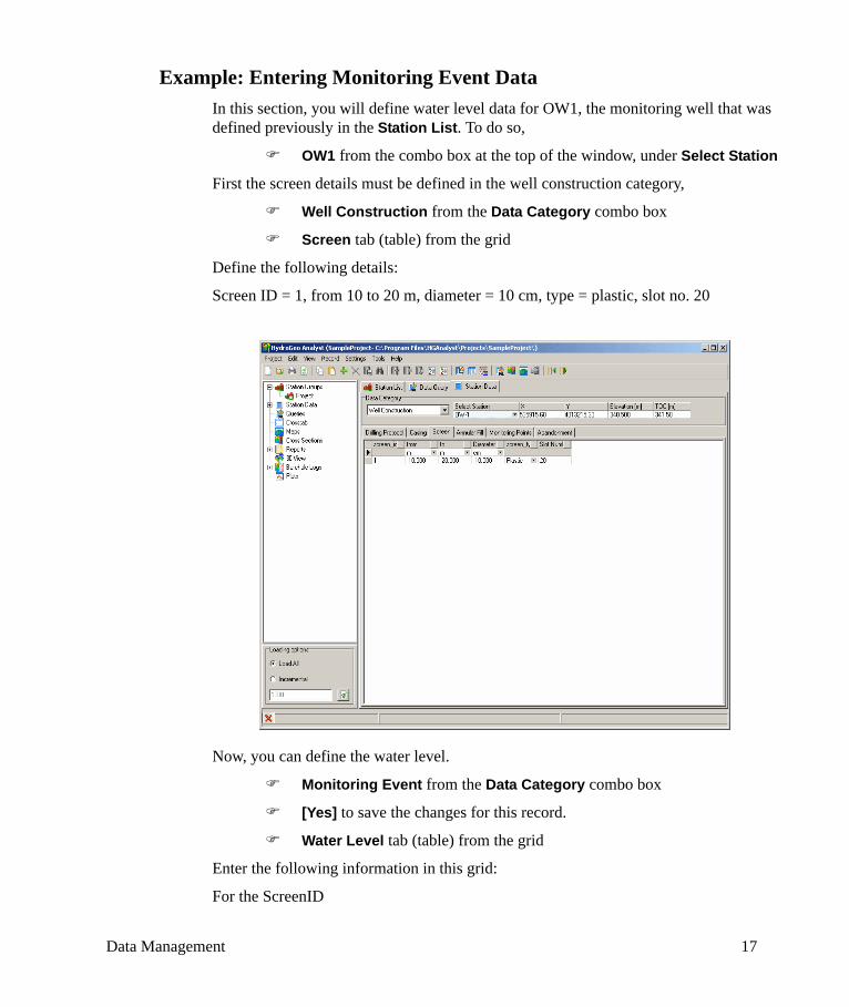
Example: Entering Monitoring Event DataIn this section, you will define water level data for OW1, the monitoring well that was defined previously in the Station List. To do so,

OW1 from the combo box at the top of the window, under Select Station

First the screen details must be defined in the well construction category,

Well Construction from the Data Category combo box

Screen tab (table) from the grid

Define the following details:

Screen ID = 1, from 10 to 20 m, diameter = 10 cm, type = plastic, slot no. 20

Now, you can define the water level.

Monitoring Event from the Data Category combo box

[Yes] to save the changes for this record.

Water Level tab (table) from the grid

Enter the following information in this grid:

For the ScreenID

Data Management 17

1 from the combo box

In the Date column,

type: 5/5/2004

In the Time column,

type: 1:00:00 PM

In the Depth to Water Level (m) column,

type: 15.33


Record > Post from the main menu or press the (Post) button in the toolbar, to save the data.

The remaining fields can be left blank. Your table should be similar to that shown in the figure below:

As demonstrated here, it can be quite time-consuming to enter data manually. If the source data is available in a text file, spreadsheet, or database, it is much more efficient to import the data into the new Hydro GeoAnalyst project. This option is explained in the next section.


1.2.2 Importing Data using the Data Transfer System (DTS)Hydro GeoAnalyst allows data to be imported from a variety of sources, using the Data Transfer System (DTS). A few examples are provided below.

Example: Importing Stations from an Excel FileThe following example demonstrates how to import data using the DTS. You will import some additional borehole stations to the Sample project. (The DTS will be briefly covered in this section; for more details on this feature, please see the Project Manager chapter in your User’s Manual.

Project > Import > Data from the main menu. This will load the Data Transfer System as shown below:

In the Choose a Data Source window, create a data package and select the source file:

Package Name, and select New Package from the combo box

type: Stations in the box that appears

[OK]

(The data package will save the DTS import settings and configuration, for quick and easy recall later on).

button, beside the Specify Import File name field

In the Import File dialog,

Change the Files of type => Excel (.xls)

Data Management 19

Sample_Stations.XLS file, located in the “...\Examples” folder (located in the HG Analyst program folder). The default folder is “D:\Program Files\HGAnalyst\Examples”.

[Open]

[Next] to proceed to Step 2 of the DTS

Once the data source is provided, the next step is to match a Source table with a Destination table. The DTS provides an interface that can be used to select the destination Hydro GeoAnalyst table by first selecting the data category that contains the table and the desired destination table. Once the destination table is selected, all fields in the table will be listed for field mapping.

The source table containing the data to be imported can be selected from the list of tables on the left side of this window.


Under Source Table,

Sheet1$ (if it is not already selected) from the combo box

The DTS makes an effort to automatically match fields from the source table with those in the selected destination table. If the field names are exactly the same, the fields will be mapped automatically. Unmapped fields will appear blank; this indicates that the DTS was unable to match the source field to a field in the Hydro GeoAnalyst database. Therefore, a field must be manually selected from the available list, and mapped to the appropriate source field.

In this example, some of the fields have been detected and mapped automatically: ID, Name, X, Y, and TOC; but the Elevation field needs to be mapped manually.

NOTE: As a minimum, each source table must contain either the Station ID or Station name for each record. These fields are required to match the source data to the appropriate stations in the database.

Under the Source table,

Click on the blank field directly above TOC; this field corresponds to the Destination field Elevation. A list of available fields will appear, as seen below.

Elev from this list; this field contains the Elevations for the stations.

NOTE: The remaining unmapped fields are not necessary for this project.

Data Management 21

Next, define units for a few of the “length” type fields highlighted in the Source table (Elev and TOC). To do so, locate the Unit column under the Source table, and select a unit for the Elev field

m from this list.

Repeat this for the TOC field, as shown below.

NOTE: The units for station X,Y co-ordinates will be defined in Step 3 of the import routine.

[Next] to proceed to Step 3 of the DTS.

The next window is the Station Related Settings. In here, select the Projection Type and Units for the station coordinates in the source file.


For this example, there is no need to change the projection, since the station coordinates in the source are in the same projection system as the one defined for the project. This step also allow you to specify the destination station group.

[Next] to proceed to the last step of the DTS.

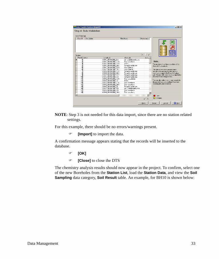
The last step of the DTS is the Data Validation window, and this provides a preview of the data to be imported. Errors or warnings, if any, will be listed along with the data.

Data Management 23

The data is checked against three conditions, namely:

• Proper Station Locations (in Lat - Long format);• Specified conditions for each field (if any); and• Data type compatibility.

The DTS converts station co-ordinates into latitude-longitude format, and displays the converted values in the Preview frame. Stations are converted and stored in the database in this format; however the station co-ordinates may be displayed in Hydro GeoAnalyst in any projection system desired (for this project, stations will be displayed in NAD 1983 UTM Zone 17 N).

By default all data marked as erroneous will not be imported. However, all warnings are ignored by default. One or more of these error messages can be selected and the data affected by those errors can either be rejected or accepted. Erroneous records will not be accepted for importing unless the errors are fixed. All values causing errors are highlighted in different colors. Red represents rejected or erroneous records; yellow represents a warning/caution for the selected records.

Each of these problematic records can be selected and edited before it can be accepted for importing. Once a record is edited, it can be accepted using the [Accept] feature for records.

For this example, there should be no errors/warnings present.

[Import] to import the data.

Read the confirmation message.


[OK]

[Close] to close the DTS

Example: Importing Lithology DataIn this section, you will import Lithology data from a file. This data will be later visualized in 2D cross sections, and with the 3D Explorer.

Project > Import > Data from the main menu.


type: LithologyData in the box that appears

[OK]




Sample_Lithology.XLS file, located in the “...\Examples” folder (under the installation folder). The default installation folder is “D:\Program Files\HGAnalyst\Examples”.

[Open]

[Next] to proceed to the next window in the DTS

In the Data Mapping window, you must select a new Destination Data Category and Table (from the right side of the window). In this case, the Lithology data will be imported to the Geologic Description category, Lithology table. Select the appropriate items from the combo boxes, as shown in the image below

Data Management 25

Under Destination,

Geologic Description for the new Destination Data Category

Lithology for the new Destination table

Under Source Table,


Next, map the fields and select appropriate units. In this example, most fields are automatically mapped, since the field names in the source are identical to the field names in the destination. However, the ID field must be manually mapped, and the units must still be selected for the length field types.

ID for the field name in the first row of the Source table.

m for the units for the From_ and To_ fields

[Next] to continue

The next window is Data Validation. If you mapped the fields correctly, then your DTS window should appear similar to the one shown below:


NOTE: Step 3 is not needed for this data import, since there are no station related settings.



A confirmation message appears stating that the records will be inserted to the database.

[OK]


The new lithology data should now appear in the project. To confirm, select one of the new Boreholes from the Station List, load the Station Data, and view the Geologic Description, Lithology table. An example, for BH10 is shown below

Data Management 27

Since the data was imported directly to the SQL Server database, it is not necessary to Post (Save) the changes.

In the next section, you will import soil chemistry data for the boreholes.

Example: Importing Soil Chemistry DataIn this section, you will import soil chemistry data from a file.

In most of the data models provided with HGA, chemistry samples must have a sample code (the field name is sys_sample_code in many database schemas). When importing the chemistry data, you need to import the sample_id first, in the Parent Tree of the database (Soil_Sample table), THEN import the chemistry data into the Soil_Result table (child table)

A unique sample code (sample_id) should be assigned for each sample; the same sample code may be used for multiple parameter analysis.

Import Sample Codes



type: Soil Sample ID in the box that appears


[OK]




Soil_sample_ID.XLS file, located in the “...\Examples” folder (under the installation folder). The default installation folder is “D:\Program Files\HGAnalyst\Examples”.

[Open]


In the Data Mapping window, you must select a new Destination Data Category and Table (from the right side of the window). In this case, the soil sample codes will be imported to the Soil Sampling category, soil_sample table. Select the appropriate items from the combo boxes, as shown in the image below

Under Destination,

Soil Sampling for the new Destination Data Category

soil_sample for the new Destination table

Under Source Table,


Data Management 29

Next, map the fields and select appropriate units. In this example, most fields are automatically mapped, since the field names in the source are identical to the field names in the destination. However, the station_name field must be manually mapped, and the units must still be selected for the length field types.

m for the units for the from_ and to_ fields

Under the Source, first row in the table,

Station_name from the combo box

[Next] to continue

[Yes] to continue, in the warning message that appears.






[OK]



The new sample codes should now appear in the project.

Now you are ready to import the soil chemistry analysis results for these sample codes.

Import Chemistry Results



type: Soil chemistry data in the box that appears

[OK]




Soil_chemistry_data.XLS file, located in the “...\Examples” folder (under the installation folder). The default installation folder is “D:\Program Files\HGAnalyst\Examples”.

[Open]


In the Data Mapping window, you must select a new Destination Data Category and Table (from the right side of the window). In this case, the soil chemistry data will be imported to the Soil Sampling category, soil_result table. Select the appropriate items from the combo boxes, as shown in the image below

Data Management 31

Under Destination,

Soil Sampling for the new Destination Data Category

soil_result for the new Destination table

Under Source Table,


Next, map the fields and select appropriate units. In this example, most fields are automatically mapped, since the field names in the source are identical to the field names in the destination. However, the station_name field must be manually mapped,

Under the Source, first row in the table,

Station_name from the combo box

Click on the result_unit field,

Use (if not already selected)

[Next] to continue

Read the warning message that appears,

[Yes] to continue.

A second warning message will appear as shown below.

[OK] to continue.







[OK]


The chemistry analysis results should now appear in the project. To confirm, select one of the new Boreholes from the Station List, load the Station Data, and view the Soil Sampling data category, Soil Result table. An example, for BH10 is shown below:

Data Management 33

Since the data was imported directly to the SQL Server database, it is not necessary to Post (Save) the changes.

Example: Importing Water Level DataIn this section, we will import water level data for each station in our HGA project.

In most of the data models provided with HGA, water levels must have an associated Screen Id. When importing the water level data, you need to import the Screen Id first, in the Parent Tree of the database (screen table), THEN import the water level data into the gw_level table (child table).

Import Screen Id


Package Name, and select New Package from the combo box.

type: Screen_Id in the box that appears

[Ok]



Change the Files of type ==> Excel (.xls)

screen_id.xls file, located in the “...\Examples” folder (under the installation folder). The default installation is “D:\Program Files\HGAnalyst\Examples”.

[Open]

[Next] to proceed to the next window in the DTS.

In the Data Mapping window, you must select a new Destination Data Category and Table (from the right side of the window). In this case, the screen id values will be imported to the Well Construction category, screen table. Select the appropriate items from the combo boxes, as shown in the image below.

Under Destination,

Well Construction for the new Destination Data Category.

Screen for the new Destination table.

Data Management 35

Under Source Table,

Sheet1 (if is it not already selected) from the combo box.

Next, map the fields and select appropriate units. In this example, most fields are automatically mapped, since the field names in the source are identical to the field name

m for the units for the from_ , to_ and diameter fields.

[Next] to continue.

The next window is Data Validation. If you mapped the fields correctly, then your DTS window should appear similar to the one below:

Note: Step 3 is not needed for this data import, since there are no station related settings.


[Import] to import the data

A confirmation message appears stating that the records will be inserted into the database.


[Ok]

[Close] to close the DTS.

Now that the Screen Id values have been imported, you can proceed to import the water level data.

Import Water Levels

Project > Import > Data from the main menu

Package Name, and select New Package from the combo box.

type: Water Level Data in the box that appears

[Ok]

button, beside the Specify Import File name field.



water_level.xls file, located in the “...\Examples” folder (under the installation folder). The default installation folder is “D:\Program Files\HGAnalyst\Examples”.

[Open]

[Next] to proceed to the next window in the DTS.

In the Data Mapping window, you must select a new Destination Data Category and Table (from the right side of the window). In this case, the water level data will be imported to the Monitoring Event category, GW_Level table. Select the appropriate items from the combo boxes, as shown in the image below.

Data Management 37

Under Destination,

Monitoring Event for the new Destination Data Category.

gw_level for the new Destination table.

Under source Table,

Sheet1 (if it is not already selected) from the combo box.

Next, map the fields and select the appropriate units. In this example, most fields are automatically mapped, since the field names in the source are identical to the field names in the destination.

m for the units for the depth field.

Remark from the last row (to map with Comment)

[Next] to continue

[Ok] to continue, in the information message that appears



.


For this example, there should be no errors/warning present.



[Ok]

[Close] to close the DTS.

Data Management 39

The water level data should now appear in the project. To confirm, select one of the Boreholes from the Station List, select the Station Data tab, and view the Monitoring Event data category, Water Level table. An example for OW1 is shown below:

Using the HGA Lab Quality Control tools, you may now perform a quality control assessment on your data, analyzing blanks, duplicates, and spike samples. This feature is outside the scope of this exercise. For more details, please see the Quality Control chapter in your User’s Manual.

1.2.3 Creating Station GroupsOnce the data has been successfully entered into the project, it may be convenient to sort the stations into logical groups. Grouping stations allows for efficient management and quick retrieval of data stored in the database.

Station groups can be created based on any criteria. Common examples include:

• Locations of the stations (e.g. locations sorted by City, Project Sites, etc.)• Station type (e.g. Monitoring Locations, Boreholes, etc.)• Purpose of Study (e.g. remediation, site monitoring)

All station groups created for a project are listed in the Project Browser under the Station Groups node. Clicking any of the sub-nodes corresponding to a station group will display the appropriate stations belonging to that group in the Station List tab.


Station Groups can be created manually or through the use of the Query Builder. The following example demonstrates how create a station group manually, containing the Borehole stations.

Example: Creating a Station GroupTo create a Station Group:

Station List tab

OW1 (ensure this row becomes highlighted, similar to the image shown below)

Record > Invert Selection. This will highlight all the Boreholes, and de-select the observation well (OW-1).

Right-click on any of the selected Boreholes, and select “Add Station Group” as shown below

Data Management 41

In the dialog that appears, enter a name for the new station group.

type: Boreholes

[OK]

The selected stations will be added to the new group “Boreholes”, and this Station Group will appear as a new node (branch) in the Project Browser. These stations will also remain in the Project Station Group.

Once the stations in a group are displayed, a number of actions can be taken based on the selection. For example, loading a station group and then activating the mapping component will automatically create a GIS layer containing all stations from this group. This option will be demonstrated later in this chapter.

1.3 Viewing Borehole Log PlotsIn this section, you will see how to create a Borehole Log Plot (BHLP) for one of the stations.

Boreholes station group

BH1 station, since this station contains data for well construction, casing, screens, etc.

Next, locate the Borehole Logs node in the Project browser.


+ beside Borehole Logs, to expand this node

Double-click on whi2 (BHLP2), to load this Borehole Log Plot template. The BHLP will appear, similar to the following figure.

This BHLP template contains a pre-defined structure with Lithology, Well Construction, and Scaling information. The BHLP Report may be exported to an XML file, printed directly, or saved in several formats including .HTM, .PDF, .XLS, etc.

For more details, please see the Borehole Logs chapter in your User’s Manual.

To proceed with this exercise,

[Close] button to close the BHLP window

1.4 Querying the DatabaseOnce the data has been successfully entered into the project, the Query Builder may be used to run queries on the station data. Queries provide the ability to search and find a specific set of data or stations, quickly and easily. Some examples of this application include:

• Finding stations located in a specific area of your site (search by X, Y location).• Searching Monitoring event data, for groundwater chemistry samples which

exceed a guideline level.• Finding all wells which exceed a specified depth

In addition, using the Query Builder you can create Data Queries that provide the data sources for:

Querying the Database 43

• Map Layers• Cross section interpretation results • Quality Control Analysis • BHLP columns• Crosstab reports • 3D plume projects • Charts • Customized Reports

Example: Querying the Database

In this example, you will create a data query that returns all stations that have soil chemistry exceedences for PCE (Tetrachloroethylene).

Follow the directions below to build a simple query:

Tools > Query Builder from the main menu, or click on the button from the toolbar. The Query Builder window will load as shown below.

Data Query as the type, in the upper-left section of the window

(New Query) button in the toolbar.


In the dialog that appears, enter a Name for the new query. For this example,

type: PCE_exceedences

[OK]

The Project Tree on the left side of the window contains the database structure, with the data categories, tables, and fields. For this example, expand the Soil Sampling category, then the Soil Result table, and locate the Chemicals field.

+ beside Soil Sampling

+ beside Soil Result

An example is shown below:

Click once on the field, and drag this field into the Conditions frame.


The selected field will be added automatically to the Query Conditions. Alternately, you may use the (Add) button (on the bottom half of the window) to add conditions, then define them manually.

Under the Conditions frame, select an Operator for the field. A combo-box with several options will appear: >, >=, <=, <, =, <>, !=, !>, !<, LIKE, IS, IS NOT, &, !. For this example,

= (equals symbol) from the combo box

Next, enter a value in the second Expression field. For this example,

Tetrachloroethylene from the combo box

In addition, add the Chemicals field to the Display fields in the upper frame.

Click once on this field, and drag this field into the Display Fields frame.

Next, you must enter the result value field. From the project tree on the left side of the window, locate the Result_Values field.

Click once on the Result_Values field, and drag this field into the Conditions frame.

Under the Conditions frame, select an Operator for the field. A combo-box with several options will appear: >, >=, <=, <, =, <>, !=, !>, !<, LIKE, IS, IS NOT, BETWEEN, &, !. For this example,

> (greater than symbol) from the combo box

Next, enter a value in the second Expression field. For this example,

type: 1

In addition, add this field to the Display fields in the upper frame.

Click once on the Result_Values field, and drag this field into the Display Fields frame.

Once the fields have been added, the Query Builder display should be similar to the one shown in the figure below.


(Generate SQL Statement) button from the toolbar at the top of the window to Generate the SQL string. If the Query string is invalid, the violating rows will be highlighted red (indicating error) or yellow (indicating warning).

(Execute SQL Statement) button at the top of the window to execute the query string.

If not already active,

SQL View > Preview tab to see the results of the Query. The results should be similar to that shown in the figure below:


(Save Query) button to save the query

[Close] to return to the main Hydro GeoAnalyst window

This query will now appear as a new node under the Queries branch of the Project Browser.

A warning message may appear, stating “Do you want to save changes made to the Station List”.

[Yes] to save and proceed.

1.4.1 Recalling and Executing QueriesOnce a query has been created, it will remain available from the main Hydro GeoAnalyst interface.

A Station Group Query will appear as a branch under the Station Group node in the project browser. The stations which satisfy the query will be automatically added to this new Station Group.

A Data Query will appear as a new branch under the Queries node in the project browser.

To see the results of a selected query, right-mouse click on the query and select Execute option. The Query results will then be displayed in the Data Query tab, as shown in the example below.


With this data query, you now have the option to generate a Crosstab query report. This feature is outside the scope of this exercise. For more details, please see the Queries chapter in your HGA User’s Manual.

If you have time-varying data for one or more contaminants in your database, you may generate data queries with these fields then generate Time Series charts. This feature is outside the scope of this exercise.

In the next section, you will create a map project, and display some of the boreholes on the map.

1.5 Mapping the DataOnce the data has been entered into a Hydro GeoAnalyst project, quite often it is helpful to relate this data to features on a base map, and create contour maps or thematic maps (Pie or Bar charts) for interpreting the data. This can be done using the Map Manager. The first step is to create a new map project.

1.5.1 Creating a Map ProjectIn this section, the Borehole stations will be loaded onto a new map project. To create a new map project,

Tools > Map Manager or right click on the Map node, and select New.

Mapping the Data 49

A prompt will appear to enter a name for the new map project, as shown below

type: Sample

[OK]

A new Map window will appear. To load the stations from Hydro GeoAnalyst on to the map project,

Layer > Load HGA Data from the menu in the Map Project window. The following window will appear.

Use this option to load Station Groups or Map Ready Data Queries into your map project.

Ensure the Boreholes Station Group is selected.

[OK]

The Set Field Precision Dialog will appear on your screen,


The Set Field Precision dialog box can be used to set the number of decimal places that appear when using the label renderer on these numeric fields. We will accept the default values.

[OK]

The Borehole Stations will then be plotted on the Map in the Map Project window, as shown below:

Note: By default, Map Manager uses the projection system that is defined in the project settings . You can change the projection system by clicking on Project > Properties, and selecting a new projection from the dropdown menu list.

In the Map Project, you may create a new map layer that contains a map image, from any of the following sources:

• Raster Images (*.BMP, *.TIF, *.JPG, *.SID, and others)• AutoCAD files (*.DWG, *.DXF, *.DGN)

This feature is demonstrated in the next section.

1.5.2 Importing and Georeferencing a Site MapAn example of how to import a map is provided below.

Layer > Import > Raster from the Map Project main menu.

Sample_Map.bmp file, located in the folder “D:\Program Files\HGAnalyst\Examples”.

Mapping the Data 51

A warning message will appear verifying that the image must be georeferenced.

[Yes] to continue.

A prompt will appear to define a name for the new site map.

Enter the name: Sample_Map_GR.bmp (where GR indicates that the image will be georeferenced).

[Save] to continue.

The Georeference window will appear as shown below.

In order to map the pixels of the image to a coordinate system, the image must have at least two georeference points with known coordinates. A third georeference point can be used to improve accuracy. However, for demonstration purpose, only two points will be used in this guide. These georeference points must be assigned as described below.

Adding Georeference PointsTo set the georeference point,

Click on the first map location where the world coordinates are known. For this image, the points for X1, Y1 and X2, Y2 are marked with an * on the map.


A Georeference point window will appear prompting for the X1 and Y1 world coordinates of the selected location. Note: The world coordinates must be in the projection system that the map project is set to.

Enter the following coordinates for this point:

X1 = 535122

Y1 = 4812839

[OK]

Click on the second map location where the world coordinates are known. This point is marked with an * on the map as X2, Y2, in the upper right corner.

Enter the following coordinates for this point:

X2 = 537252

Y2 = 4814712

[OK]

The image is now georeferenced. Next, in order to use the full map window, you must maximize the extents.To do so,

Options > Full Region in the Georeference Window; the window should now appear similar to the figure shown below

Mapping the Data 53

[OK] in the Select Region Window. This will close the Georeference window.

[OK] in the File Attributes window.

[OK] in the Confirmation window, stating the image was georeferenced successfully.

The Raster Image now appears as a new Map Layer in the Map Project. However, it will appear at the top of the Layer Manager panel, and as a result, will hide the Boreholes station group layer. Therefore, the new map layer must be moved down. To do this,

Using the mouse, drag-and drop the SiteMap layer below the Boreholes layer.

After doing this, the Boreholes station group layer will be displayed on top of the site map, as seen in the figure below.


At this time, feel free to experiment with the properties of the Boreholes layer, by modifying the symbol properties.

Adding LabelsTo add labels to the Boreholes,

Boreholes layer

Layer > Renderer from the main menu of the Map Project window. The Renderers dialog will appear.

Mapping the Data 55

(Add) button to add a new renderer, and the following dialog will appear with the available Renderer types.

Label Renderer

[OK], and the following dialog will appear.

type: Label for the Name

Name for the Field Name

[OK] to close the Renderer type window

[OK] again to close the Renderers window

The stations will now be identified with the appropriate label.

1.5.3 Creating a Contour MapContour maps may be created to quickly visualize a measured result value (soil or groundwater concentrations) or elevations (surface or water table) data. In this example, you will create a contour map of the surface (ground) elevations.


Boreholes layer from the Layer Manager panel to ensure that the data layer is active. If the layer is active, it will appear bolded in the Layer Manager Panel.

Layer > Create Contours > Create Contours HGA from the Map Project main menu. A Contours dialog will appear, as shown in the following figure:

Elevation from the Choose Field combo box at the top of the dialog

type: ContourMap in the Name textbox.

Settings for the Contour Line contour type

In the Contour Line Settings dialog,

type: 2 for the Contour Interval

[Ok]

[Create]

The contour map will now show up as a new map layer in the map project. The contour map properties may be modified, including the line thickness and color. To do so,

Mapping the Data 57

ContourMap layer in the Layer Manager panel, to make this active.

Layer > Properties from the menu. The following dialog will appear:

Feel free to experiment with the line properties. It may be helpful to change the color and line thickness. Once you are finished:

[OK] to apply the new properties.

The map project with the contour map should now be similar to the one shown in the figure below.


1.5.4 Creating a Color Shade MapColor Shade maps may be created to further visualize a measured result value (soil or groundwater concentrations) or elevation (surface or water table) data. In this example, you will create a color shade map of the surface (ground) elevations.

Boreholes layer from the Layer Manager panel to ensure that the data layer is active.

Layer > Create Contours > Create Contours HGA from the Map Project main menu. A Contours dialog will appear, as shown in the following figure:

Elevation from the Choose Field combo box at the top of the dialog

Contour Line checkbox to disable this contour type.

Color Shade checkbox to enable this contour type.

type: ColorShadeMap in the Name textbox.

Mapping the Data 59

Settings for the Color Shade contour type

The Color Settings Renderer allows you to define different colored zones/ranges according to their specific interval of values. You can use the [Classify] button to set the number of intervals. HGA will automatically divides the available range of values into that number of equal intervals. Use the [Ramp] option to define the color palette.

You can experiment with different classifications and color schemes. For demonstration purposes, lets keep the default settings.

[Ok] button to exit the Color Settings dialog.

[Create] button

A message will display indicating that the color shade map was successfully generated.

[Ok] button


By default, the new color shade map layer will appear at the top of the Layer Manager panel and as a result, cover up the other layers. From the Layer Manager panel,

Using the mouse, drag-and-drop the color shade layer onto the Boreholes layer.

Disable the SiteMap_gr.bmp layer by unchecking its visibility checkbox.

When used with contour lines, the color shade map layer allows you to easily visualize detailed information about the surface elevation in our area of study (shown below).

Mapping the Data 61

1.5.5 Defining Cross Section LinesThe Map Manager also provides an interface for drawing and defining the locations of cross-sectional lines. Since the Map Manager provides a plan view of station data, it is a simple task to draw lines in the location(s) of the desired cross-section(s). Cross Section lines are defined using the CrossSection Line option. A line is drawn through the desired stations, then a buffer distance is provided to specify which stations to include. A large buffer distance will result in selecting stations further away from the line; a small buffer distance means that only stations close to the line will be selected. Only the stations within this buffer distance become highlighted and selected for the cross section interpretation. The cross section may then be created using these selected stations.

An example is provided below on how to define a cross-section line in the Map Manager.

Before proceeding, hide the ContourMap, as it will no longer be needed.

ContourMap layer from the Layer Manager panel

Remove the check mark for the Visible status for this layer. This layer will now be hidden from the view. Do the same for the ColorShadeMap layer.

Boreholes layer from the Layer Manager panel, to ensure that this layer is active.


HINT: In order to activate the cross-section options, a layer that contains Station data must be selected.

(Cross-Section Line) button from the toolbar

Place the mouse cursor near the top left corner of the map, and click once with the left mouse button to start the line.

Drag the mouse across the map, to the bottom right corner of the map, passing in between some of the stations as you draw the line.

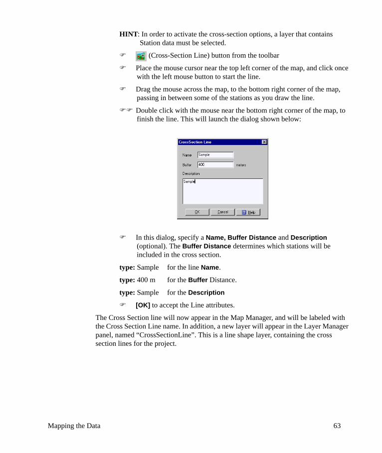
Double click with the mouse near the bottom right corner of the map, to finish the line. This will launch the dialog shown below:

In this dialog, specify a Name, Buffer Distance and Description (optional). The Buffer Distance determines which stations will be included in the cross section.

type: Sample for the line Name.

type: 400 m for the Buffer Distance.

type: Sample for the Description

[OK] to accept the Line attributes.

The Cross Section line will now appear in the Map Manager, and will be labeled with the Cross Section Line name. In addition, a new layer will appear in the Layer Manager panel, named “CrossSectionLine”. This is a line shape layer, containing the cross section lines for the project.

Mapping the Data 63

Those Borehole stations that lie within the 400 m Buffer Distance will be selected (as indicated by a red circle on top of the station’s symbol) and included in the cross-section. (The Buffer Distance is projected perpendicular to the cross-section line).

1.5.6 Creating the Cross SectionOnce the cross-section line is defined, the corresponding cross-section can be created:

Tools > Create Cross Section from the main menu, or click on the Show/Create Cross Section button on the toolbar (this button is located beside the Cross Section line button).

A confirmation dialog will appear.

[Yes] to create the cross-section; the name assigned to the cross-section line will be used as the cross section name.

[Yes] at the Select Surface dialog box. (This option allows you to generate topography lines from contour layers.)

The cross-section editor opens the selected cross-section, and displays the stations and related information. The cross-section shows projections of the borehole’s lithologic columns on the cross-section plane. By default, the top of model layer 1, (ground surface topography), will be drawn in for you.


The Cross section window should be similar to the one shown below:

NOTE: Yours may be slightly different depending on the location of the cross section line, and the stations which were selected along the line.

In the Cross Section editor, locations for layers must be interpreted, and drawn manually using lines or polygons; layer types may be Geological, Hydrogeological, or Model. The process of drawing layers is described in the next section.

For more details on some of the other features of the Map Manager, please refer to your HGA User’s Manual.

1.6 Interpreting and Viewing Cross-Sections

1.6.1 Drawing Geologic Cross-Sectional LayersOnce the desired stations have been loaded into the Cross Section Editor, the layer locations must be interpreted. To draw Geologic layers, the polygon draw tool must be used, and the polygon must be digitized manually using the mouse.

To draw a geological cross-section layer, follow the directions below:

Interpreting and Viewing Cross-Sections 65

Click once in the box beside Geology from the Layer Manager panel, to activate this layer, and make it editable. You should have two check marks beside Geology, as shown in the image below; the first check mark indicates the layer is visible; the second check mark indicates the layer is editable (in edit mode).

Choose the (Polygon) button from the toolbar

Place the mouse cursor near the top left corner of the map, near 340 m on the y-axis.

Click once on the left mouse button to add a vertex and start digitizing the polygon in the desired direction;

Add more vertices by clicking on the left mouse button at desired locations. Move the mouse cursor to an interval on a desired station; the mouse cursor will snap the vertex of the polygon to the nearest station interval. A vertex can also be added anywhere on the cross-section by clicking on the left mouse button.

HINT: When drawing interpretation polygons, use the soil patterns displayed in the boreholes as a guideline for the layer location; however, since it is a


interpretation, it does not need to exactly match up with the interval locations.

Double click anywhere on the cross-section using the left mouse button to close the polygon; the Geology Layer Pattern window will appear:

In the dialog that appears, enter a Name for the layer, a brief Description, and select a soil Pattern. If the geologic layer you have just digitized in the current cross-section has already been created, you may select it from the combo box, instead of typing a new name. Click on the blank area beside Pattern to load the pattern options, as shown in the following figure:

Select a pattern, (sand is located in the top-right corner of this dialog),

[OK]

[OK] once more


The polygon will be filled with this pattern; an example is shown below.

Repeat the same sequence of operations for other layers within the active cross-section. The result will be a layered structure of the geological domain. The cross-section may contain some gaps where polygons do not completely touch adjacent polygons; this can be easily fixed by selecting a vertex on a polygon, and using the pointer tool to re-position the vertex. Alternately, gaps between polygons can be filled by using the Link Vertex option.

Once a layer is created in one cross-section, it will be available for selection in all other cross-sections that you create for your project. Altering the properties of a given layer will be reflected in all cross-sections.

Once the desired view has been obtained, the cross section may saved. To do so,

File > Save from the main menu, or click the (Save) button from the toolbar.

Then, remove the editable status for the Geology interpretation. To do this,

Edit check box beside Geology in the layer control.

For information on drawing model layers or hydrogeological interpretations, please see the Cross Section Editor chapter in your User’s Manual.

In the next section, you will view the cross section in 3D Explorer.


1.6.2 3D Visualization (Fence Diagrams)The Hydro GeoAnalyst 3D Explorer allows for visualizing multiple cross sections in three-dimensions, and combining cross sections for creating fence diagrams. In addition, you may visualize transient contaminant plumes for one or more chemicals in your project.

To load a cross section into 3D Explorer,

View > View 3D from the main menu, or click on the (View 3D) button from the toolbar.

In this dialog you may select which cross-sections, surfaces, or 3D plumes should be added to the 3D project.

[OK] to accept the default settings.

This will load the 3D Explorer window, as seen in the following figure.

The Geologic Interpretations will be displayed by default. To better visualize the fence diagram, make the following changes to the view and grid orientation:

At the top of the 3D window, locate the Vertical Exaggeration factor field.

type: 10 for the Vertical Exaggeration


<Enter> on the keyboard.

Next, rotate the grid so that you can view the fence diagram from the side. To do so, locate the Navigation Tools at the bottom of the window (these tools contain 3 tabs that control the Rotate, Shift and Light Position options). By default, the Rotate tab will be selected, and will contain three slider bars, one for each of the X, Y, and Z axes.

X Slider bar and slowly drag this to the left.

Watch the 3D grid rotate as you do this. Stop when you have reached a satisfactory side profile of the fence diagram.

Next,

Y Slider bar and slowly drag this to the right.

Watch the 3D grid rotate as you do this. Stop when you have reached a satisfactory side profile of the fence diagram.

Finally,

Z Slider bar and slowly drag this to the right.

After rotating the grid, your 3D image should be similar to the one shown below.


The full capabilities of 3D Explorer are not discussed in this chapter. For details on how to use 3D Explorer, please refer to the HGA 3D-Explorer chapter in your User’s Manual.

File > Save from the main menu to save the 3D project

Once the desired view has been loaded, the 3D image may be loaded into the Report Editor. To do so,

File > Print from the main menu, or click the (Print) button from the toolbar. This will load the Report Manager, where the 3D view may be customized, or printed as is.

In the next section, you will create a few sample reports. Before proceeding, close the 3D Explorer:

File > Exit from the main menu

1.7 Preparing ReportsThe Reporting component included with the Hydro GeoAnalyst package allows for creating reports containing any data from the database, in addition to borehole log plots, time series plots, maps, cross-sections, and 3D views.

1.7.1 Creating Data Reports from GridsSelect any grid, then press the print button on the toolbar. If a template is available, there will be a prompt to select a template. For example, if you want to print the station list,

Station List tab

(Print) button from the toolbar. A print template may be selected, if desired.

[OK]

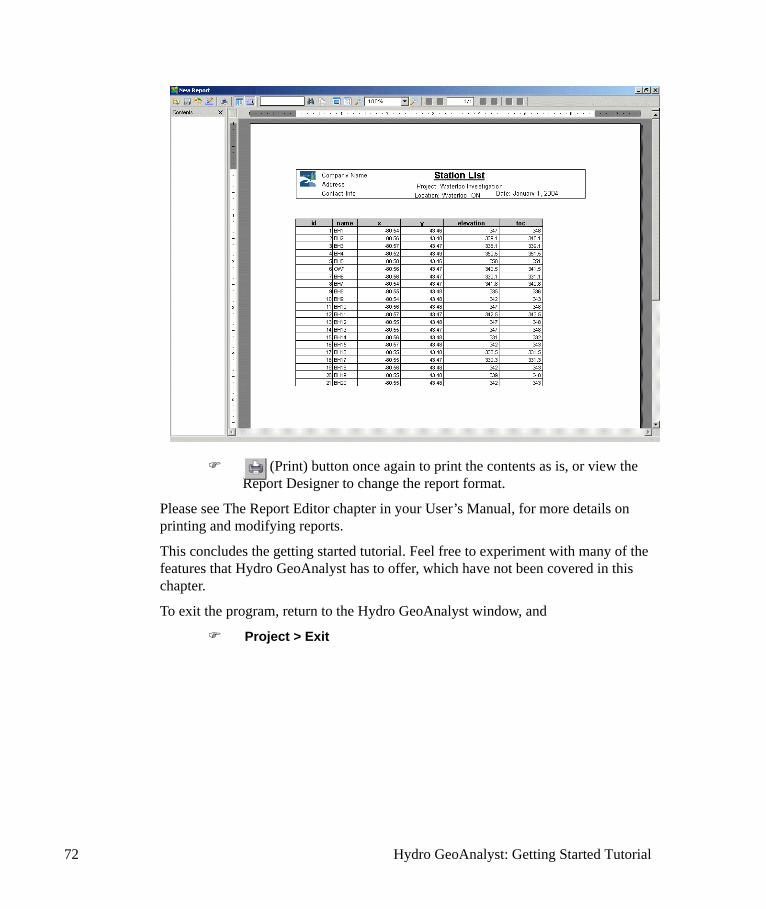
This will load the Report Viewer. An example is shown below.

Preparing Reports 71

(Print) button once again to print the contents as is, or view the Report Designer to change the report format.

Please see The Report Editor chapter in your User’s Manual, for more details on printing and modifying reports.

This concludes the getting started tutorial. Feel free to experiment with many of the features that Hydro GeoAnalyst has to offer, which have not been covered in this chapter.

To exit the program, return to the Hydro GeoAnalyst window, and

Project > Exit


Date post:	16-Mar-2018
Category:	Documents
Upload:	dangnhi
View:	230 times
Download:	5 times

Hydro GeoAnalyst: Getting Started...

Documents